1
Industrial Electrical Engineering and Automation
CODEN:LUTEDX/(TEIE-5160)/1-62/(2002)
The Design of a Simulator for
the Automation Industry
Jan-Olof Sivtoft
Department of Industrial Electrical Engineering and Automation
Lund University
The design of a simulator
for the automation industry
Maj 2002
Jan-Olof Sivtoft, E94
Handledare Tetra Pak, Istvan Ulvros
Handledare IEA, Gustaf Olsson
Abstract
The development of new technologies forces the industry to develop new products cheaper and
faster. Every advance has it own opportunity window and if you are too late, a lot of money and
time are wasted. In the automation industry the product development process can last over a year
and therefore several project are running side by side but only a few will survive to the end.
Tetra Pak R&D in Lund has studied this problem during the past few years and their aim is to find
out if there is a possibility to use some kind of simulator instead of expensive test machines. This
master thesis is one step in that direction and its main goal is to construct as simulation environment
consisting a soft-PLC and a mechanical visualization program. The main problem is how these two
programs should communicate during a simulation. The PLC will control the model built in the
visualization program and react from signals produced from the model. Therefore a simulation core
has been designed and one possible solution to the communication problem is explained.
The core is developed in Visual Basic and a test model is a common part taken from any ordinary
filling machine. Finally the controller program is designed in ladder code.
Contents
1
1.1
1.2
1.3
1.3.1
1.3.2
2
2.1
2.2
2.2.1
2.2.2
2.2.3
3
3.1
3.2
3.3
4
4.1
4.2
4.2.2
4.2.3
4.2.4
4.2.5
5
5.1
5.2
5.3
6
6.1
6.2
6.3
A
A1
A2
A3
A4
A5
A6
A7
A8
A9
A10
A11
Preface..................................................................................................................................... 3
Introduction............................................................................................................................ 5
Why building a software simulator ......................................................................................... 5
Goals of the thesis.................................................................................................................... 5
Limitations and methods ......................................................................................................... 6
Results...................................................................................................................................... 6
Report outline .......................................................................................................................... 6
Simulation environment ........................................................................................................ 8
Total structure.......................................................................................................................... 8
Components ............................................................................................................................. 9
FrameworX (FX) ..................................................................................................................... 9
Working Model 3D (WM3)................................................................................................... 10
Visual Basic (VB).................................................................................................................. 11
Use of communication mechanism ..................................................................................... 12
What is OPC .......................................................................................................................... 12
FrameworX built-in OPC-server and its OLE Automation interface.................................... 12
Working Models OLE Automation interface ........................................................................ 14
Simulator design .................................................................................................................. 16
Description of the simulator .................................................................................................. 16
Code design in Visual Basic.................................................................................................. 18
Simulation_Main class........................................................................................................... 19
Component classes................................................................................................................. 22
Simulation modules ............................................................................................................... 23
Arrangement in FrameworX and Working Model ................................................................ 25
Test Model ............................................................................................................................ 28
Description of the model ....................................................................................................... 28
The monitor ........................................................................................................................... 31
The controller ........................................................................................................................ 32
Conclusions........................................................................................................................... 35
Result ..................................................................................................................................... 35
Possible improvements .......................................................................................................... 35
Future developments.............................................................................................................. 36
Appendix............................................................................................................................... 37
Nomenclature......................................................................................................................... 37
Form Simulation_View ......................................................................................................... 38
Class Simulation_Main.......................................................................................................... 41
Class Input_Controller........................................................................................................... 43
Class Arm .............................................................................................................................. 44
Class Sensor........................................................................................................................... 45
Module Simulation_FX_Connection..................................................................................... 46
Module Simulation_WM3_Connection ................................................................................ 48
Module Simulation_FX_To_WM3 ....................................................................................... 50
Module Simulation_WM3_To_FX ....................................................................................... 51
Controller code ...................................................................................................................... 53
References.............................................................................................................................. 57
2
Preface
Finally this work has been completed and I want to thank all people involved during this project
both at Tetra Pak R&D in Lund and Department of Industrial Electrical Engineering and
Automation at LTH. I would like to tank Bo Hellberg and Lennart Christensson at Tetra Pak for
their help during my time at Tetra Pak. A special thanks for their encouragement and patience goes
to Istvan Ulvros, Tetra Pak and professor Gustaf Olsson.
Finally I would like to thank my girlfriend Tove who has been supporting me all along this work.
3
4
1 Introduction
1.1 Why building a software simulator
In the automation industry it usually takes a long time to develop new machines. There are many
steps in a development cycle that all costs a lot of money. If the development time could be
shortened, the costs would be reduced. Far from every machine design idea leads to a complete
machine. If an idea could be rejected earlier, it would save unnecessary development costs.
In at least one stage during the development cycle it is necessary to build a test machine. This test
machine is expensive and without any doubt there must be corrections made of this machine several
times due to incomplete design. If the number of errors could be reduced before starting using the
real machine, it will reduce the development time, spare parts and of course the costs.
So there are several reasons why a research and development department would like to build a
simulator instead of a real machine in the early stages of a development cycle. In a simulator we can
build a model of the machine and we can test it without breaking anything. It is much easier to do
changes in the simulator than in the real machine. By using a simulator the control program could
be tested several times long before it is first tested on the real machine.
As we can see there are many reasons to build a simulator. It helps to shorten development time,
reduce cost due to errors and spare parts, and makes it easier to do changes and so on. But why
don’t we do this every time we want to build a machine? One answer to that question is that there is
no software available, designed for this purpose. So in this thesis I will try to design a simple
simulator out of known software and make it work.
1.2 Goals of the thesis
The main goal was to make a simulator and to simulate a part taken from a filling machine. The
simulator must handle signals both ways between itself and a controller. The simulator must also
contain some kind of visualisation and this is done by some software supplied with graphical tools.
This means that the visualiser must allow to be controlled from outside and be able to send signals
back when some certain criteria are met. To achieve this there were a few other minor problems
that had to be solved first.
Programs use different ways of communication with other programs. Therefore a communication
link between them must be designed. The programs can’t work together in real time, since they are
located on the same computer. The time must be divided between them and this must be controlled
in some way.
An object must be constructed to simulate different parts of a real machine. How these objects are
designed depends on several things but the most important thing is that we must be able to reuse all
objects and that there must not be any limitations to add new objects to the model. In other words,
the simulation core should not have to be changed when a new object is added.
5
1.3 Limitations and methods
The simulator was limited to two programs available in the commercial market, one being the
controller and the other the simulation of the machine. The two programs are FrameworX from GEFanuc, (FX) which is a soft PLC and Working Model 3D Motion from MSC Working Knowledge,
(WM3) which is a mechanical motion simulation software.
As the work went along, it turned out to be difficult to establish communication between the
programs. The main reason of this was that in the early stages in my work, FrameworX was only
available in a beta version without proper manuals. Especially the OLE Automations for Process
Control, OPC, documentation was missing which made it very difficult to connect the two
programs together. Another problem was that the final version of Working Model 3D was delivered
very late during the limited thesis working time. Therefore the work had to be focused on the minor
problems and there were no time left in the end to build a complete machine simulator as intended.
The thesis is limited to establish communication between the programs, control the data flow
between them and build a small demonstration model to show how the simulator is supposed to
work.
In the beginning of the work, time had to be spent to learn and understand the basics around
FrameworX and Working Model 3D. Internet was used to find information about OPC. Missing a
lot of primary information trial and error had to be used a lot during the work. When
documentation then was available is become easier and the communication was improved quite fast.
Then it was possible to focus on building a few objects and test model so it became possible to
demonstrate the simulator function. It finally worked!
1.3.1 Results
The main goal was to build a complete simulator and that goal was achieved. However, to build a
complete machine part as intended, failed. But the principles are shown in the small test model and
it is only a question of available time to build a more complex test model.
1.3.2 Report outline
The report is divided into three parts. The first part describes briefly the software used and the
communication protocols. This is done in Chapters 2 and 3. The second part, Chapters 4 and 5,
deals with simulation methods and test model. Finally the last chapter summarises the result of the
work.
To fully understand how this simulation works the reader should have some knowledge about object
orientated programming in Visual Basic. Those just interested in the simulation method may look
directly at Chapter 5
6
During the second part there will be some written code among the text. This code is taken from the
final code created in Visual Basic. But some details are left out and sometimes there is no real code,
just some text notes. However, the complete code is printed in appendices A2-10.
7
2 Simulation environment
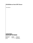
2.1 Total structure
The simulator consists of a soft-PLC, communication link and a mechanical simulation program.
The control program resides inside the PLC and it communicates with OPC, OLE Automations for
Process Control trough an OPC-server. The soft-PLC used is FX-Control from FrameworX, GEFanuc and from now on, called FX. But the simulator is not bound to FX and it can be replaced by
any other soft-PLC that uses OPC to communicate. But FX has an advantage in having a built-in
OPC-server and all communication between FX and the OPC-server is handled automatically by
FX. Therefore, when referring to FX the OPC-server is included.
F
OP
OPC
Serve
AP
“FX”
V
“VB”
AP
WM
“WM3”
Figure 2.1 The model consist of three parts. To the left: The soft-PLC and an OPC-server, from now on called FX.
Middle: Visual Basic and both API, referred as VB. To the right: Working model 3D, shorten toWM3.
The communication link consists of two OLE Automation interfaces, refereed as API and the
simulator core written in Visual Basic, hereafter named VB. The main task for the communication
link is to transfer and translate signals from FX to the mechanical simulation program, but it also
contains functions, such as starting and stopping the simulator. Finally it also has a monitoring
function, which allows us to se how the signals change during a simulation.
One API is providing VB with an interface to communicate between OPC and VB. Through the
interface object is created and connected between FX and VB. All signals controlling the simulation
come from FX and are transferred to mechanical simulation, except from a few simulator signals.
The other API is providing VB with an interface to the mechanical simulation program. Through
these interface signals is collected from the mechanical model and transferred to FX. Of course the
interface also provides the model with signals sent from FX.
Finally the mechanical simulation program is built to visualise the machine movements. This
simulator is using Working Model 3D Motion from MSC Working Knowledge. This program will
be referred to as WM3 from now on. WM3 has a large number of possibilities to build advanced
models but our model is very simple and its main purpose is to show the idea behind the simulator
8
2.2 Components
As mentioned in the previous sections there are totally six components in the simulator. They can
be divided into three parts according to fig 2.1. The “FX” part consist of FX and the OPC-server as
shown in the left box in the figure. Below in this chapter there is an overview of FX and the OPCserver is discussed in chapter 3. The “VB” part or the core of the simulator consists of all written
code in VB. Both API are imported and used in the code so they are treated as a one in VB. The
middle box contains both API and VB. Both API will be described a bit further in chapter three and
below a very brief overview to VB. The third part consists only of WM3 that also will be discussed
later in this chapter.
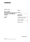
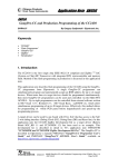
2.2.1 FrameworX (FX)
FX is a soft-PLC, which integrates development and execution of a controller. It also provides a
graphical tool to build a HMI that can monitor the process.
The program supports tools such as Ladder and SFC according to IEEE 1131. It also has a tool
chest where many predefined objects are stored. Most of them has a graphical interface and can be
used when building a HMI.
Figure 2.2 Screenshot of FX-control.
In the very early stage of the thesis the graphical tool was explored to reveal if it could be used as a
visualisation tool of the machine. But then the model would only consist of a schematic model and
most important only in two dimensions. Also add some advanced algebra to solve all mechanical
properties and it would be a thesis of it own.
9
Actually there are two different programs that can be executed, FX-control or FX-view. The
differences between them are that FX-control contains the development environment and FX-View
consists only of the HMI and the executing controller. It is said before that there is a built-in OPCserver to FX, actually there are two of them, one each to FX-control and FX-view. Every time any
of those programs is started the corresponding OPC-server is also started.
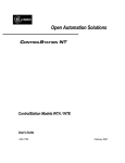
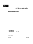
2.2.2 Working Model 3D (WM3)
WM3 is a 3- dimensional simulation program for mechanical models in motion. It’s a pure
simulator tool where the model of the “real” machine is simulated. The model is build by many
different bodies and constraints with different degrees of freedom. Each body can have different
geometrical and physical properties and they can also have initial speed and acceleration.
Movements are described by functions and tables and of course the impact the environment
consisting of all other bodies. There are also some defined objects such as motors, springs and
pistons that can be used to create more dynamic models. Momentum and forces can be applied
anywhere and can be used as initial conditions. Other greater feature is that it is possible to import
models form other CAD-tools and convert them into WM3 models.
Figure 2.3 Screenshot of WM3
Several properties can be controlled during the simulation through inputs. It is actually this feature
that makes it possible to control the model from an outside source i.e. a controller. WM3 has a very
simple script language, which mainly consists of the if-function, mathematical function and some
signal generators. But together with inputs it is quite simple to control properties during the
simulation of the model.
10
It is also possible to collect information from the model or, as we see it, signals that can be sent to
the controller. This is done by using an output that is an object that calculates a value during each
frame using information from the model properties together with the script language. Here the
signal generator functions that can extend a signals duration are especially helpful. But, even if
outputs give us a way to get a certain information from the model, they are not used in the
simulator. The reason is that it is easier to directly use the API and acquire the information from the
model.
Visualisation of the model is very powerful. It is possible to look at the model from anywhere and
zooming down to small details. When a simulation is performed it remains in the memory until a
new simulation is done or if it is deleted. Rerunning the simulation will increase the visualisation
speed and it can be done from any angle and zooming. Finally it is possible to export a simulation
as a video clip that can be shown in other tools.
However, one major feature is missing in WM3 which was a part of is predecessor Working Model
2D. Instead of giving a value to the side of a cube and the let other bodies refer to that side, it must
be set to a numerical value. This makes it very time consuming to edit fundamental body values in a
model and the whole model must be revisited. The same problem occurs when objects are placed in
the model. Fore example if two objects should be three radiuses apart it would be very helpful to
use the first objects reference point and then add three radiuses for the second one.
One other thing to understand is that WM3 is not currently powerful enough to perform real-time
simulation even if it is working stand-alone. Of course this is also a hardware issue and therefore
there are a great possibilities to improve performance in the future.
2.2.3 Visual Basic (VB)
The simulator core is written in Microsoft Visual Basic 6 as a part of Microsoft Excel tool. The core
serves as a “glue” between WM3 and FX, taking care of timing issues and signal handling, but also
has a simple monitor window where the user can follow the signal flow between FX and WM3
VB is an object-orientated language with is focused on the user and his interaction with the
program. In an application it is the user who controls the flow by actions throw the GUI, normally
by the mouse or keyboard. VB contains classes, which has methods and properties that can perform
operations and set attributes in the object. VB works with three components, class modules
(classes), modules and forms. Each class contains information about an object and its methods and
properties. The modules contain a set of procedures that should be executed each time they are
called. Finally, the forms represent the visible part in VB. We can create buttons, textboxes, and
lists and so on in order to communicate with the program.
Besides this, there are several APIs that can be added to the VB-environment that can be used to
create objects to control other applications without implementing that object. We just create an
instance of the object and it is ready to use.
11
3 Use of communication mechanism
3.1 What is OPC
OPC stands for OLE for Process Control and it is a standard protocol to transmit data and I/Osignals between programs running within the Windows environment. OPC is built upon two of
Microsoft’s technologies, OLE and DCOM and it’s also designed and optimised for industrial
applications. It is developed by a non-profit organisation, the OPC-Foundation, which provides free
specifications for developers.
The main reason behind OPC was to create a protocol, which allows different automation
applications to work together independent of any manufacture specifications. There are many
benefits, both for consumers and manufactures. The consumers are no longer limited to one
manufacturer and the system they provide. The consumer can freely change the controller and
choose one that suits his needs without changing the whole system. The manufacturers only have to
provide one communication-interface and therefore their development process will be shortened.
Thus they can concentrate on the application and compete with their products in a larger market.
OPC uses the concept of servers and clients. The server is connected to a controller and provides
data to the system throughout clients on their request. Since the server simply is a program it can
run in parallel on the same computer as the controller. The clients are data-consumers but they can
also send information to the server, typically trough a HMI to control a process.
There are two ways a client can get information from the server. The easiest but an inefficient way
is polling. The client asks the server and will receive an answer directly. But the client doesn’t
know when a value has changed so it has to ask repeatedly. Another way is to let the server notify
the client when a value has changed. Then the client can respond by acquiring the value form the
server or by reading all values of interest at the moment.
3.2 FrameworX built-in OPC-server and its OLE Automation interface
As mentioned earlier FX has a built-in OPC-server. The advantage of this is that every signal
defined in the controller is registered in the server directly. The only thing VB needs to know is the
name of the server and some additional information if they are located on different machines.
Lets take a closer look how we connect the OPC-server from VB. Of course the API must be
installed and registered in VB before any of the code below will work.
First an object that will handle the OPC-server at the client is created. It is then connected to the
OPC-server named “fxControl.OPCServer.1” which is the name of the server started by FXControl. The third row in the code below creates an OPC-Groups object. Each signal in the server
must belong to a group. The advantage with groups is that you can create an event to each group
that will fire as soon as one of the signals in the group changes its value. This is a very useful way
to notify the client that something has happened among all the signals in a specific group. The
12
object OPC_Groups handles all groups created in the program and before we can do anything a
group must be created.
…
Set OPC_Server = New OPCServer
OPC_Server.Connect ("fxControl.OPCServer.1")
Set OPC_Groups = OPC_Server.OPCGroups
Set myGroup = OPC_Groups.Add("myGroup ")
…
After the group two properties are added, IsActive and IsSubscribed must be set to true in order to
acquire data from the OPC-server, continuously. Before we can register the signals we have another
level of object in the OPC-server to handle. OPCItems is an object that keeps a collection of items
together inside a specific group.
…
myGroup.IsActive = True
myGroup.IsSubscribed = True
Set myItems = myGroup.OPCItems
Set myCommand = myItems.AddItem("#Command", myGroup.ClientHandle)
…
Then finally the signal is added to the OPCItems object. Here it is important that the signal name is
spelled exactly as in the server i.e. case sensitive. Otherwise a signal is registered in the server but if
there is no corresponding signal name in the server, no error is reported.
Now we can use the signal in our program and we can read and write to the signal. Writing to the
signal is simple. We use the method write and the value is written to the OPC-server. Of course a
value must be of correct type i.e. Boolean, integer, char but otherwise it’s easy.
myCommand.Write (setValue)
myCommand.Read
k = k+ myCommand.Value
Reading a value is done in two steps. When the read method is called it collects the value from the
OPC-server and stores it in the object in a property named value. After that the value is accessed by
calling the property. The value will remain the same until the read method is called again.
13
3.3 Working Models OLE Automation interface
In this section we will take a closer look at WM3 and the API we are using to communicate
between VB and WM3. Before we can read or write to WM3 we must create an object in VB so we
can accesses its properties. Following code does this.
Set App = GetObject(, "WM3D.Application")
Set Doc = App.ActiveDocument
The App object contains a reference to the WM3 program and the Doc object contains a reference
to the model in WM3. The Doc object is our link to the model and through this we can access
almost everything in the model. We can control the whole simulation or the colour of any body in
the model. But to do this we must create a link to each specific object we want to control. In the
simulator we are most interested to get values from bodies and to set new values to inputs.
Lets take a closer look how we acquire a reference to a specific body object. The first step is to get
references to every body form the Doc object. Then we must know the name of the body in WM3.
Here are two possibilities, first we can use WM3 predefined name fore each body which is
“body[index]” where index corresponds to the order the bodies where created in WM3. Second we
can give each object in WM3 a name and use that name to find it from VB.
Set CollectionOfBodies = Doc.Bodies
Set myBody = CollectionOfBodies.Item(myName)
In the code above myBody now contains a reference to a specific object named myName in WM3.
There is no need to go into each detail of each property but a body object has 4 methods and 6
properties. Two of these methods are GetConfig and SetConfig, which can be used to change the
three-dimensional configuration of the body object. However one of the properties is of great
importance to the simulator. This is the IsInterferingWith property that returns true or false if the
body is interfering with any other body i.e. this property alone acts as a sensor. Unfortunately this
property requires a name of an other body to check if they are interfering. This means that one has
to loop through every body of interest before one knows the answer. But the great benefit is that
there is no need to calculate any geometry to reveal the answer.
Besides bodies there are motors, inputs and outputs that are of interest, but they all work in a similar
way so there is no need to go deeper into that.
Now let’s go back to the Doc object. In order to control the simulation there is a method
RunTo(FrameNumber) which is very helpful when simulating. Upon calling the method the
simulation will start and continue until it reaches the frame number. During this time VB is halted
and will resume first when WM3 is done. The frame number is kept by the Doc object, so in order
to make a good simulation you increase the frame number by one each simulation cycle and the
precision in the simulation is mainly determined by the frame rate i.e. frames per second.
14
15
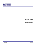
4 Simulator design
4.1 Description of the simulator
To begin with, we have two industrial programs running on the same computer and using the same
resource, the CPU. A third program is also executing in the same environment and is responsible for
synchronising information between the programs. When we are simulating we need to calculate
how it would be in a real machine and extract information from those calculations and pass the
information between the two programs. If we knew from the beginning what we want to do and
have all the inputs ready then it would be best to run and complete the first program. The
information could them be passed to the second program and after it is completed we would have
the result of the simulation. But, this is not sufficient for simulations in the automation industry
where we want to pass information between the programs several times during runtime. So instead
of running each program completely, we run them a little bit at a time and in between information
are shared. So, the main idea behind the simulator is that the available time in the computer is
divided in small fractions and that each simulation program is running in parallel. Between the time
periods the third program executes and transfers parameters between the programs.
Though, it is interesting to know how a computer handles several programs at the same time we
should not concern us anymore about that. Instead we will look how the different programs work
together and thereby understand more about the simulation method. At first, we will look at them,
as we would like to do in a simulation.
Let us start with the simulator. Before the VB-script can be executed we must start WM3 and FXView and load the simulation model into the environment. After that we start the VB-script and we
are then ready to run the simulation from FX-View.
Initialize simulation
Setup connections
Control simulation
WM3D - application
creates WM3D objects in VB
FX-Control / OPC
register variables in OPC
Continue
Read from OPC
Step one frame
Read from
Run one scan
Write to WM3D
In WM3d
WM3D
in FX-Control
Control simulation
Hold, Continue
Quit
End simulation
Figure. 4.1 The simulator structure
16
When the VB-script is started it begins with initialising two objects, one, which is the WM3D
application and the other, is the OPC-server in FX. These object are necessary because they contain
the simulation variables that must be transferred between the programs to make the simulation
work.
The WM3D-application object contains the whole model and every object can be manipulated from
the VB-script. However, most of the manipulation is done during the second stage, set-up
connections, before the actual simulation begins. During simulation the only external changes in the
model are changing colours at some objects i.e. turning their visibility on or off. But to be able to
read some values from the applications object we must create a corresponding object in VB. Of
course we must send control signals, inputs, to the simulation but those signals should not be treated
as a part of the model.
If we look at the OPC-Server we have a similar problem. But instead of creating a corresponding
object in VB we only have to register a variable in the OPC-Server and connect it to the
corresponding variable in the controller. So before the actual simulation can start we must initialise
all objects and register all variables that we need for the simulator to work. This is also done in the
VB-script in two separate modules, which are executed in the set-up connection phase.
Now we are ready to run the simulation. Each cycle in the simulator consists of one scan in the
controller and one frame calculation in WM3D. We also have to transfer control signals in both
directions during one cycle. In the model we begin each cycle by reading the current controller
value in the OPC-server. They are then transferred to WM3D, which then executes one simulation
frame. Next, we read the out signals from WM3D and write them to the OPC-server. Finally, we
execute one scan in the controller.
The question that should be raised after this, is how we can assure that only one scan is executed in
the controller and how do we know when it is done? The answer is that the controller is equipped
with a command option which aloud us to run only on scan in the controller and then freeze it. After
this scan, it also changes a value of one of its internal variables, #command. This variable is
accessible throughout the OPC server and connected to a VB-variable during connectionconnection phase. When the controller executes, VB is idle and is waiting for an event from the
OPC-server. This event is trigged each time the controller changes the value of #command. To
summarise: the controller is signalling when one scan is done and VB will continue to execute.
Actually we have the same problem for WM3D but it is solved much easier and was discussed in
3.3.
17
4.2 Code design in Visual Basic
The simulator consists of several different components, but the main functionality lies in the VBscript. Therefore we will take a closer look at the structure and code in VB. The complete code is in
Appendix A2-10, but some extracts are shown below to make it easier to understand the design and
functionality.
In previous chapters we have talked about objects and how we need to create them to be able to run
the simulation. But before we can create them they must be designed and programmed in VB. We
also need to know which objects are needed and how they work together, which also can be seen in
figure 4.2.
Figure 4.2 Form, class and module dependency in the simulator
In our model we use one class for the simulation core and three classes represent different “real”
components in the machine. Of course a machine normally contains more than three components
but for now three is sufficient. To be able to simulate a more realistic machine more objects need to
be designed. The design of each such object totally depends on how the object is supposed to work
and how accurate the model would be. However, it is really easy to add a new class, i.e. a new
component to the model. Of course they have to be connected to the model but we don’t have to do
any modifications in the simulation core, which is one of the goals of the thesis.
18
A closer look at the components object reveals that they have two types of methods in common,
initialisations methods and runtime methods. The initialisations methods are responsible for
connecting, registering and settings of a specific component. These methods are executed in the
beginning of each simulation and may also be called when a simulation is reset. The runtime
methods are used during a simulation and their task is to read or write signals between FX and
WM3D. They are normally called once each scan during the simulation. We will discuss these
classes in more detail in 4.2.2.
4.2.2 Simulation_Main class
The simulator core consists of one class Simulation_Main and four modules. The class itself
controls and runs the simulation. The modules contain all information about all used signals
between FX and WM3D. The reason we use four modules is that then we don’t need to change
anything in the class when we are creating a new simulation model. Everything that belongs to the
model itself is controlled from the four modules.
The main program in this model is actually very small and simple. Most of the simulators
functionality lies in the Sim object that is an instance of class Simulatin_Main . When we start the
VB-program, a form is activated and this form creates the Sim object. It also throws an event that
executes the UserForm_Activate() method.
Private Sub UserForm_Activate()
Sim.Init_Sim
Sim.Setup_Connections
Sim.Sim_Control.Write (8)
End Sub
The Sim object must first be initiated, i.e. create all object used by the simulator such as the OPCserver object, WM3D-application object and connect main control signals. Next all signals used by
the model must be attended. This means that every signal defined in the
Simulation_FX_Connections and Simulation_WM3_Connections modules are created, initiated and
registered. Finally, signal is sent to the PLC which to run one scan.
Besides this, the form is drawn on the screen. The form is monitoring all signals connected between
FX and WM3. During each cycle every signal is updated and this is a very helpful tool when we
want to study the simulators behaviour.
The buttons to control the model are created in FX but they are also connected to the Sim object
through the OPC-Server. The buttons, Start, Stop and Reset controls the PLC and the program that
lies inside. Each one of these buttons is throwing an event when they are pushed causing VB to
start, stop or restart the simulation.
As mentioned above Sim is the core of the simulator and therefore we will take a closer look at is
Sim_Init method. There are five main tasks for Sim_Init to do. First, import and create an object,
App, that corresponds to the WM3D model. WM3D must be running and the active document is the
simulation model, which is reset.
19
Public Sub Init()
Set App = GetObject(, "WM3D.Application")
Set Doc = App.ActiveDocument
Doc.Reset
App.Activate
…
After that an object, OPC_Server, as discussed in chapter 3.2. is created that will handle the OPCserver
…
Set OPC_Server = New OPCServer
OPC_Server.Connect ("fxControl.OPCServer.1")
Set OPC_Groups = OPC_Server.OPCGroups
…
Third, a number of signals are registered in the OPC-server that will handle the start and stop of the
simulation. For this reason a group, Sim_Control_Group, is added to the OPC_groups object. It is
also a good idea to set some properties for the group. Most important are the IsActive and
IsSubscribed properties as mentioned in 3.2. A third property, UpdateRate, is also set. This controls
the rate at which an event from the group may be fired. This rate should match the general frame
rate for the simulator.
Next we create an OPCItems to hold the individual signals within the group. Since we only have
five signals we could manage with one group, but I have chosen to create two groups. One contains
the PLC control buttons, i.e. start, stop and restart signals, and the other one contains simulator
signals. After this is done we are ready to register the items or signals to the OPC-server. So by
adding them to the Main_Group_Items object, we create a VB-object at the same time.. The only
requirement is the name of the corresponding signal in FX-control.
…
Set Sim_Control_Group = OPC_Groups.Add("Sim_Control_Group")
Sim_Control_Group.UpdateRate = 250
Sim_Control_Group.IsActive = True
Sim_Control_Group.IsSubscribed = True
Set Sim_Control_Items = Sim_Control_Group.OPCItems
Set Sim_Control = Sim_Control_Items.AddItem("#Command", Sim_Control_Group.ClientHandle)
Set PLC_Ready = Sim_Control_Items.AddItem("PLC_Ready", Main_Group.ClientHandle)
Set Main_Group_Items = Sim_Control_Group.OPCItems
Set Main_Control_Start = Main_Group_Items.AddItem("Main_Control.SwitchOutput[0]", Main_Group.ClientHandle)
Set Main_Control_Stop = Main_Group_Items.AddItem("Main_Control.SwitchOutput[1]", Main_Group.ClientHandle)
Set Main_Control_Reset = Main_Group_Items.AddItem("Main_Control.SwitchOutput[2]", Main_Group.ClientHandle)
PLC_Ready.Read (2)
While Not (PLC_Ready.Value = 1)
PLC_Ready.Read (2)
Wend
End Sub
20
The most important signal for the simulator is the #Command signal in the PLC which allows us to
control the simulator by starting, stopping and do a single scan in the controller. The object
corresponding to #Command is named Sim_Control in VB. There is an other signal in this group,
PLC_Ready that is used in the beginning to check if the controller is up and running.
As soon as all five signals are registered, the event driven method
Sim_Control_Group_DataChange is called when anyone of those signals changes its value. So, to
start the simulation we just have to push the start button in FX.
Public Sub Sim_Control_Group_DataChange
If Main_Control_Start Then
Call OneScan
End If
If Main_Control_Restart Then
Call Reset
End If
End Sub
Now we have reached the core in the simulator, the One_Scan method. If we compare the code with
figure 4.1 we recognise that the four boxes in the middle row corresponds to the five lines in the
method. The remaining two lines are updating the VB-form, so every signal can be monitored. This
is done every time signals are parsed from FX or WM3D.
Public Sub OneScan()
Simulation_Fx_To_WM3.Scan Me
Call Simulation_Veiw.Update
Frame = Frame + 1
Doc.RunTo (Frame)
Simulation_WM3_To_FX.Scan Me
Call Simulation_Veiw.Update
Sim_Control.Write (8)
End Sub
OneScan begins with passing all signals from the controller to WM3D. Then one frame is executed
in WM3D. During that time period the VB script is halted and will resume first when WM3D is
done. Next signals are transferred to the controller and finally one scan are executed in the PLC.
Now VB is idle and waits for something to happen. And as soon the PLC has done one scan the
#Command will be set to 0 and the Sim_Control_Group_DataChange method is activated and
another cycle is started.
21
4.2.3 Component classes
There are two things a user of the simulator has to do in VB to be able to run a simulation. One of
them is creating component classes and the other is connecting them to the simulator.
When we want to design a new class corresponding to a real component there are several things to
look at. First of all we want the object to act as a real one but on the other hand it must be
reasonably easy to use. Depending of the type of simulation there is a trade-off between accuracy
and speed. If we want better performance of the object it usually takes more time to calculate the
simulated parameters of the component and vice verse.
However in our model we already has a program, WM3D, taking care of the mechanical simulation.
What we have to do is extracting information from the model in WM3D and translate it to useful
signals in FX-control. Some properties are easy to gain; others take some calculations to obtain.
Fortunately, the API to WM3D gives us several ways to extract information, which isn’t supported
by the internal script language in WM3D. Exploring all possibilities using script and API together
would probably give us quite good objects, but that is not one of the main goals of this thesis.
Therefore only three components are modelled and in a “quick and dirty” fashion way. The most
important has been to show that a controller can control WM3D during runtime.
There are three classes, each one representing one type of component in the simulation model.
These are Sensor, Arm and InputController. They all have one method, init, in common. This
method is called during Set-up and is responsible for connecting a VB variable to WM3D. During
the simulation each component has its own methods depending on its functionality. Next we will
discuss each component in brief.
Sensor component
A sensor can be one many different types, optic, heat, pressure etc. Depending of the model,
different sensors will be implemented. The sensor modulated in our model is a contact sensor,
which gives a true value when something is in contact with the sensor, otherwise false. There are 34
sensor objects that together act as 28 sensors in the model. The idea behind each sensor is when two
objects are in contact with each other a signal should be set to true. Now, how do we detect this? If
we look at WM3D one way would be to calculate the distance between specific points in each
object. When the distance is smaller than a certain value the objects are in contact with each other.
If the objects are symmetrical it would, in general, be fairly easy to make the detection. But if they
were not, we would have to a bit more complex algorithm, which would take some CPU-time to
execute and thereby slowing the simulation down and also increase the time to build the model.
Instead of doing all this by ourselves, we use a method for body objects in the API for WM3D.
This method, IsInterfering, reveals if two specific objects are in contact. In WM3D the sensor
consists of one single body. The size and position of the body depends on the specific model.
Unfortunately, this method has two bodies as input parameters and therefore we must test every pair
of bodies that are of interest. If any pair is true the sensor should be set to true otherwise false. But
this method is much easier to use than calculate the distance.
22
The sensor object has three methods, init and CheckPower and CheckPulse. The difference between
the last two ones is that CheckPulse only is set to true during the first executed frame when the two
objects are in contact. CheckPower remains true during the whole time while the objects are in
contact. The init method is used during connection and contains the sensor body and the trigger
body. During the simulation CheckPower and CheckPulse are called every time signals are parsed
from WM3D to FX.
Input_Controller component
The Input_Controller component is a simple object. It passes an integer value to an input object in
WM3D that could be used in many ways. I our model an input controls the speed of a motor. The
motor has three levels 0-2 that mean stop, half and full speed. To set the value a method, setInt is
implemented and the value from is parsed to the input object. Besides this method Input_Controller
has three more, init, start and hold. Start and Hold actually sets the value 1 and 0. Init is used during
setup and it has one parameter, a WM3D input object.
Arm component
Finally, the Arm component, which basically is the same as an Input_Controller, but it only, has
two levels. So it is fair to say that it is more like a binary controller, and that properly would be a
better name. But it uses reversed logic which means that set is zero instead of one and vice verse.
Besides init it has two other methods, named Grip (zero) and Drop (one), which makes it easier to
use the component because one does not have to bother about the reversed logic.
4.2.4 Simulation modules
Besides the main class we have four modules that are strongly connected and works together with
the main class. Two of them, Simulation_FX_Connections and Simulation_WM3_Connections
handle the initialisations of the signals and they are called once in each simulation. The other two,
Simulation_Fx_To_WM3 and Simulation_WM3_To_Fx are called once each scan during runtime
and transfer the signals between the programs.
They all have in common that the builder of the simulation model must edit these modules. For each
signal or group of signals, depending on design, in the simulation model the builder must program
the four modules according to their use.
The “Connections” modules contain two methods, connection and reset. Set-up is called when Sim.
Setup_Connection is called in the beginning of the simulator execution. Connection is responsible
for connecting a signal between FX and WM3D. This means, create an object corresponding to a
signal in the OPC-server and register it. And of course create an object corresponding to a
component in WM3D and initiate it.
23
If we start looking at Simulation_FX_Connections, the builder must declare the object and connect
it to a signal in the OPC-server. This is done in the same way as we introduced the PLC_Ready
signal earlier. All signals are declared as Public and there is a naming convention, which states that
every object related to the OPC-server should begin with “FX_”. If it is a signal all the following
letters are written in upper case, otherwise they are written in lower cases, but the first letter in each
word is still in upper case. If it were an input to the OPC-server the letters IN_ will be added to the
object name and of course the name of an output object would be FX_OUT_. When Set-up is called
the signal is registered in the OPC_Server and ready to be used. In the code it would look
something like this
Public FX_Test_Group As OPCGroup
Public FX_Test_Items As OPCItems
Public FX_IN_TESTSIGNAL As OPCItem
Sub Setup (Sim As Simulation_Main)
Set FX_Test_Group = Sim.OPC_Groups.Add(“Test_Group_Name”)
Set FX_Test_Items = FX_Test_Group.OPCItems
Set FX_ IN_TESTSIGNAL = FX_Test_Items.AddItem("OPC_SIGNAL_NAME”,
FX_Test_Group.ClientHandle, , , ,)
End Sub
It is important to notice that the OPC_SIGNAL_NAME must be written exactly i.e. case sensitive
as in the controller. Otherwise it will not be found in the server. The other method, reset, is much
simpler because the only task it has is to reset the value to the initial values of the component.
The other module, Simulation_WM3_Connections, is a bit more complicated. Of course we have to
declare the object but we also might have to declare some extra variables to support, depending how
the component is designed. One example is when we use the sensor component. Besides the sensor
object we need a variable to store the result of an OR function between a group of sensor. The
reason behind this is the implementation of the sensor. As discussed in the previous section the
ChechPower function works between two bodies. If we want a sensor to react upon more bodies we
must test each pair. An other way to deal with this could be done with an alternative implementation
of the Sensor component. Instead of one trigger body we could have entered several bodies, but the
work of the computer would remain the same. Let’s see how the sensor placed at the end of the
conveyor is modulated. First, a look at Simulation_WM3_Connection
Public WM3_OUT_CONVEYOR_END(5) As New Sensor
Sub Setup(Sim As Simulation_Main)
…
WM3_OUT_CONVEYOR_END(0).Init Sim, "body[239]", "body[233]"
WM3_OUT_CONVEYOR_END(1).Init Sim, "body[239]", "body[234]"
WM3_OUT_CONVEYOR_END(2).Init Sim, "body[239]", "body[235]"
WM3_OUT_CONVEYOR_END(3).Init Sim, "body[239]", "body[236]"
WM3_OUT_CONVEYOR_END(4).Init Sim, "body[239]", "body[237]"
…
24
Here each container (body[233]-[237]) acting as a sensor and will react upon contact with
body[239] with is the real sensor. But we want the sensor the give us a signal when any of the
containers are in contact with the sensor. So, by using the OR function we can retrieve a single
value that we can parse along to the controller. This is how it is implemented in
Simulation_WM3_To_FX
Public conveyor_end As Boolean
Sub Scan(Sim As Simulation_Main)
conveyor_end = False
For I = 0 To 4
conveyor_end = conveyor_end Or WM3_OUT_CONVEYOR_END(I).CheckPower()
Next
FX_IN_SW_CONTAINER_READY(0).Write (conveyor_end)
…
We can see that the same naming conventions apply, except that FX_ is substituted against WM3_.
One other major difference is that the object (in this case Sensor) has methods, which is called
instead of the set statement. Once again it depend on how the component is designed. In this case
we start by calling the init method, which basically connects the object to an object in WM3D.
The last two modules are called during runtime. One of them contains the code that transfers the
signal value from FX to WM3. The other module is taking care of the signals in the opposite
direction, from WM3D to FX. They both contain a method named Scan, which is called once in
each simulation cycle.
4.2.5 Arrangement in FrameworX and Working Model
In this section we will take a closer look at some special arrangement that must be done in FX and
WM3D in order to make the simulator to work. First of all we must make sure of that both
programs have the same simulation speed i.e. the frame rate in WM3D and the scan rate in FX. This
could and should be done from the Sim Objects sim_init method. However, for some unknown
reason this hasn’t been implemented in the simulator and instead it has been done manually. It
should be quite easy to implement and in a full working simulator this must be done.
If we look at it in the “quick and dirty” way we begin with setting the scan rate variable. It should
be set to a value no less than 50 ms even if the PLC is capable of handling scan rates down to 10
ms. Instead the limit is based on WM3D capacity and therefore 50 ms are recommended as a
minimum value. In the model have chosen 250 ms to avoid a slow simulation.
Scan rate in FX corresponds to frame rate in WM3D but instead of assigning the time interval
between each scan we assign the number of calculated frames per second. A scan rate of 50 ms
corresponds to a frame rate of 20 frames per second. Even if it quite easy to calculate this value it
should be done during the execution of sim_init to avoid any miss configuration.
25
Besides actually building the model in WM3D we can do some settings to improve the simulator
speed. One way is to remove unnecessary calculations among some graphical objects. For example,
we can turn off collision detection for those objects that can never be in contact with each other.
There are several other possibilities to improve the simulation but then one really has to know how
WM3D works in detail to take advantage of those methods.
In FX, or more precisely in the controller, there is one signal in the program that belongs to the
simulator. The signal, PLC_Ready, was described in section 4.2.1 and its main purpose it to tell VB
that the controller is up and running and ready to start. There will be a closer look at this in chapter
5 when the ladder code is examined in more detail.
26
27
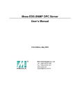
5 Test Model
5.1 Description of the model
In the previous chapters we have focused on the simulator, but we also need something to simulate.
For that reason a simple test model, the machine, has been designed, fig 5.1. The main purpose is to
show how the signals from FX can control the machine in WM3D and of course the other way
around. In brief the machine consists of two wheels, one conveyor and a number of grip arm
stations symmetric placed around the wheels edge. This could very well be a part taken from a
filling machine form the packaging industry. There is one small wheel with 3 arms and a larger
wheel with 10 arms.
Figure 5.1 A simple graphical overview over the test model.
A package is first transported on the conveyor, and then picked up by a grip arm on the small
wheel. After three-quarter of a turn it is released to the larger wheel, which controls the package for
almost one turn before the grip arm drops the package and it disappears. The conveyor and the
small wheel act as a synchronisation module to the large wheel, which will fill and close the
package.
If we look at one package and describe what the machine is supposed to do, we have the following.
A package arrives at the beginning of the conveyor and is transported along the line until it reaches
the end of the conveyor. Here we need some kind of sensor (1) telling the controller that a package
is ready for the small wheel. The wheels are running at continually speed so we need a second
sensor (2) to tell when the grip arms are in position to pick up the package. When the controller
receives the signal, it responds with a signal to the grip arm to grab the package. Actually it is the
grip arm that sends a signal when it has reached the sensor and this is how the controller knows
which grip arm should grab the package. The package then moves along the small wheel until it
reaches the transfer point to the large wheel. Here the controller receives another signal (3), which
means that the package is in position to be released to the large wheel. In the same way the large
wheel has a sensor (4) at each grip arm. The controller then responds with one signal to the grip arm
at each wheel, so the transfer of the package could be complete. Now the package will move almost
28
one turn at the large wheel before the grip arm receives a signal (5) to release the package and it
will disappear.
29
Figure 5.2 A closer look over the sensors placement.
In a perfect machine there wouldn’t be any problem with delays or lost signals. Or the wheels
would always be synchronised. But what happens if a signal is lost? In a real machine there could
very well be some problems between the two grip arms attached to the two wheels. The controller
program will not release the package from the small wheel if the signal from the receiving grip arm
is lost. Instead it will keep the package and continue. What will happen then? The package will
continue and eventually crash into the waiting package on the conveyor. Of course this is not
acceptable. Instead a sensor (6) a bit further on the turn will sense the package and an emergency
drop will be performed. To test this during simulation there is a button in the monitor window,
which removes a signal from the controller so the package will continue.
In same way the grip arm on the large wheel would sense that there is no package in the grip and
the controller program should prevent any filling or other activities round the large wheel when
there is no package in place. In the model there is no action around the large wheel so the controller
program doesn’t bother about that, but there is a release sensor (5) just before the grip arm is going
to get a new package from the small wheel.
30
5.2 The monitor
To watch the simulation there is a simple monitoring tool. It was the last thing implemented in the
simulator and in a “quick and dirty” way. However it fulfills its purpose even if it could be
improved a lot. As we can se in fig. 5.2 there is a window placed besides the FX.view so we can se
all signal changes but still be able to control the simulator. The monitor is written in VB and is
updated each time signals are transferred in any direction.
A minor error in the monitor is that there is a mix of Booleans and integers but they really mean the
same, false means zero and true means one. As mentioned earlier, signals labelled OUT_ is signals
from FX and signals labelled IN_ are signals to FX or as it says in the monitor from WM3. SW
means the small wheel and LW the large wheel. There are three arms on the small wheel implying
that there are three columns after the signals name and ten arms around the large wheel.
Fig 5.3 FX-view and the monitor, side by side
Besides monitoring all signals we can also put in some failure in the simulation. When active we are
overriding the IN_LW_CONTAINER_READY signal and the transfer between the wheels never
occurs. Instead we will be able to see that the IN_SW_EMERGENCY_RELEASE signal works as
it should.
31
5.3 The controller
The control program in the simulation is quite simple and its main purpose is to show that it is
possible to control a model in WM3. All development of the controller program is done in FX. The
program is built in ladder and SFC and the full program can be found in Appendix A11. To be able
to understand the simulation better a brief explanation of how it works comes next.
Fig 5.4 The controller described in SFC
First we have the SFC, which shows the different states that the machine can be in. There are 5
different states in the chart and almost all transitions are controlled from the main menu in FXView. When the controller is started we start in the state named “Program_Init” where the
initialisation takes place.
Before we explain the flow further a few words about how the SFC chart works are in order. The
dark grey boxes are the different states in the flow. Each state has a name and those boxes with
rounded corners with the same name as a state mean that the flow will jump to that state. The
remaining light-grey boxes have a link to a yellow box, which contain the name of those actions or
subroutines that are executed when we are in a certain state. Before each name there is a letter ‘N’
or ‘P’. The label P means that the subroutine is executed only at the first scan after it enters a state.
This is useful for initialisations of variables. The ‘N’ label means that the subroutines are executed
32
every scan until it leaves the state. Each subroutine is written in ladder and these are found in
Appendix. Between states there is a condition to fulfil before a transition is made. In this flow a
transition takes place when the variables value is true or if it is an integer greater than zero.
In the chart we can se that there are three variables, which control the transitions in the chart.
Main_Control, is an object in FX-View that controls the simulation status. The user of the simulator
can start, stop and reset the simulator from FX-view. This corresponds to three Boolean attributes to
Main_Control where SwitchOutput[0] is the start button and SwitchOutput[1] is the stop button and
finally SwitchOutput[2] is the reset button. A second object in FX-View, Skip set-up is controlling
weather we should skip the initialisation sequence, Motor_Setup, when running the test model. The
actual reason for this control is that it takes several seconds to go though this sequence and to save
some time during every test this was an easy way to do a short cut. Finally there is a transition
condition, Motor_Setup_ready, which isn’t controlled from FX-View. Instead this signals becomes
true when Motor_Setup is done.
Now, lets get back to the flow. As mentioned before there a five states in the machine, and all of
them have at least one subroutine linked to them. To simplify it even further, we say that the
Initialisation, Motor_Setup, Start_Machine and Stop_Machine subroutines are so easy that they
don’t need any further explanation. The only thing they do is to change some variables value and
this can be seen in the ladder code in Appendix A11. Instead we will concentrate on the
Run_Machine subroutine.
In section 5.1 the model was described and there we saw that the machine consists of 13 grippers
placed around the wheels. When we run the machine each arm has it own piece of ladder code and
they all run independently of each other. Each piece is encapsulated into an object and the
Run_Machine therefore consists of 13 objects of the same type. Instead of printing the ladder code
here, lets look at the functionality through an equivalent state-diagram, shown in fig 5.5.
Fig 5.5 An
equivalent state-diagram over the grip arm
33
There are 4 states in the diagram and it starts in S4. There are two requirements to meet to move to
S1. First there needs to be a container in position to be picked up. Second, the arm needs to be at the
right place. If both these criteria’s are met, the container is picked up, i.e. the output signal to the
arm is set on and the arm should grab the container. Next, we wait for a signal that we are in
position to deliver the container and that takes us to state S2. Finally we wait for a signal from the
receiver, which takes us to S3 and then directly back to S4. If something goes wrong there is an
emergency drop signal that will take us back to S4 and the container is dropped immediately.
Since the container is transferred between the small and the large wheel these must be synchronised.
They must have the same lead-time and the grip arms must be in correct position for at transfer to
occur. For that matter there is a subroutine, Motor_Setup, which will set the wheel in right position.
This is done by running each motor at a lower speed until they reach a senor. When both wheels
signals that they are in right position both motors will continue in full speed.
34
6 Conclusions
6.1 Result
There are three major results to point out from this thesis. First and of course the most important is
that the idea behind the simulator structure works. It was possible to connect these two programs
with help of a third tool and let the simulator work in accurate time. The real drawback was that it is
far from real-time simulation.
Second point is that if both programs would have used the same communication system i.e. OPC
we would have had a much simpler and better core. Instead of a lot of connection modules we could
connect the signals directly to each other and the core should only contain the timing mechanism
and the monitor. But this is something the industry can work on by pushing the software
manufacturers to supply them with better tools. Originally WM3 wasn’t designed to handle external
signals during simulation and therefore there was no need for the manufacturer to integrate any
common communication interface like OPC, but now there is a reason.
Third point is about designing the model and core code as efficient as possible. Even if we will get
faster computers they cannot make up for everything. We need to think carefully how the logic
should be structured in the simulator and how the code can be optimised, independently of where it
is located, i.e. in the core or in Working Model. If the script language in WM3 would have been a
bit more powerful we could have smoother calculations and the core wouldn’t have to do anything
else besides controlling the flow.
Then we may ask ourselves, if WM3 is the best program for this purpose?
6.2 Possible improvements
Besides changing the hardware, which can improve the simulation speed, there are a few things to
do to the simulator in general.
First, all signals are hard coded into the four VB modules, which takes some time and is
inconvenient. It should at least be reduced to one module. Instead each object should have some
more method that takes care of all initialisation and connection in a more automatic way.
The core should be replaced by stand-alone program, perhaps written in Java or C++. This should
provide a faster transmission between FX and WM3. One problem here is that there is no API for
C++ or Java available but since there is a VB-API it shouldn’t be any problem to generate one for
C++.
We could also improve the simulation of failure by adding a property to each signal. This property
could contain the fail rate of the signal. The rate could determine how often a signal change would
be lost or randomly changed.
35
There are some overall simulation properties like frame rate and scan rate that should be controlled
from the simulation main instead of changing them separately inside FX and WM3.
A great improvement would be a connection tool where we could map signals from FX to WM3
and vice verse. There is some kind of support for this through the VB-API between OPC and VB
but between the VB and WM3 it must be implemented from scratch. To achieve this in a simple
way all logic that is performed in VB to support WM3 should be moved to WM3. The drawback
here is that WM3 script language is limited, as mentioned in 2.2.2, but newer versions might
provide better functions and a deeper insight into what can be done with the script may overcome
this.
6.3 Future developments
When we have a stable and functional simulation core there are several possible expanding tools to
consider. Below there is a list with several different tools with a brief explanation. They are not
ordered in any particular way.
Graphical construction tool – This would make the simulator much more user friendly and easier to
build the model and understand the simulation.
Libraries with objects – Each new object constructed in the simulator should be added in the library
structure in order to build up a powerful toolbox.
Report generator – If we want to run longer simulations we must have a tool that can summarize
the simulation.
Finally, a quick look in the systems performance monitor, at the particular computer we used,
reveals that it is WM3 that consumes around 75% of the CPU capacity during a simulation. So in
order to have a good simulator WM3 must be improved quite a bit. One way could be to use two
computers and separate WM3 from the rest. But this is a hardware issue and as mention before
changing the hardware can increase the simulation speed enormous.
36
A
Appendix
A1
Nomenclature
API
CAD
CPU
DCOM
FX
GUI
HMI
I/O
IEEE
OLE
OPC
PLC
SFC
VB
WM3
Application Programming Interface
Computer Aided Design
Central Processing Unit
Distributed Component Object Model
FX-Control
Graphical User Interface
Human Machine Interface
Input Output
Institution of Electrical and Electronic Engineers
Object Linking and Embedding
OLE for Process Control
Programmable Logic Controller
Sequential Flow Chart
Visual Basic
Working Model 3D
37
A2
Form Simulation_View
This form contains the monitor and is also the starting application in Visual Basic. When
the form is activated the simulation core is started. Each time here is a transport of value
the Update method is called. Beside the quit button, which ends the application there is a
distortion button that removes a signal to simulate a failure.
Public Sim As New Simulation_Main
Private Main_Control As Boolean
Private Sub Distortion_Click() // Toggles distortions
Sim.Interference = Distortion.Value
End Sub
Private Sub Quit_Button_Click() // Ends application
Sim.CloseSim
Set Sim = Nothing
End Sub
Private Sub UserForm_Activate() // Executed on activation
Sim.Init
Sim.Setup_Connections
Sim.Sim_Control.Write (8)
End Sub
Public Sub Update() // Updates monitor values
// The sensor at the conveyors end
IN_CONVEYOR_END.Caption = conveyor_end
// The out signal the griparm
FX_OUT_SW_HOLD_CONTAINER_0.Caption = FX_OUT_SW_HOLD_CONTAINER(0).Value
FX_OUT_SW_HOLD_CONTAINER_1.Caption = FX_OUT_SW_HOLD_CONTAINER(1).Value
FX_OUT_SW_HOLD_CONTAINER_2.Caption = FX_OUT_SW_HOLD_CONTAINER(2).Value
// The sensor which signals if there is a package ready on the conveyor
FX_IN_SW_CONTAINER_READY_0.Caption = FX_IN_SW_CONTAINER_READY(0).Value
FX_IN_SW_CONTAINER_READY_1.Caption = FX_IN_SW_CONTAINER_READY(1).Value
FX_IN_SW_CONTAINER_READY_2.Caption = FX_IN_SW_CONTAINER_READY(2).Value
// The sensor which signals if the arm is in position to grab a package at the small wheel
FX_IN_SW_ARM_AT_INPUT_0.Caption = FX_IN_SW_ARM_AT_INPUT(0).Value
FX_IN_SW_ARM_AT_INPUT_1.Caption = FX_IN_SW_ARM_AT_INPUT(1).Value
FX_IN_SW_ARM_AT_INPUT_2.Caption = FX_IN_SW_ARM_AT_INPUT(2).Value
38
// The sensor which signals if the package is in position to be released to the large wheel
FX_IN_SW_ARM_AT_OUTPUT_0.Caption = FX_IN_SW_ARM_AT_OUTPUT(0).Value
FX_IN_SW_ARM_AT_OUTPUT_1.Caption = FX_IN_SW_ARM_AT_OUTPUT(1).Value
FX_IN_SW_ARM_AT_OUTPUT_2.Caption = FX_IN_SW_ARM_AT_OUTPUT(2).Value
// The sensor which signals if there is an arm on the large wheel in position to receive a package
FX_IN_SW_RECEIVER_READY_0.Caption = FX_IN_SW_RECEIVER_READY(0).Value
FX_IN_SW_RECEIVER_READY_1.Caption = FX_IN_SW_RECEIVER_READY(1).Value
FX_IN_SW_RECEIVER_READY_2.Caption = FX_IN_SW_RECEIVER_READY(2).Value
// The sensor which signals if the package isn’t released in a normal way
FX_IN_SW_EMERGENCY_RELEASE_0.Caption = FX_IN_SW_EMERGENCY_RELEASE(0).Value
FX_IN_SW_EMERGENCY_RELEASE_1.Caption = FX_IN_SW_EMERGENCY_RELEASE(1).Value
FX_IN_SW_EMERGENCY_RELEASE_2.Caption = FX_IN_SW_EMERGENCY_RELEASE(2).Value
// Motor and conveyor speed controls
FX_OUT_SW_MOTOR_SPEED_.Caption = CStr(FX_OUT_SW_MOTOR_SPEED.Value)
FX_OUT_LW_MOTOR_SPEED_.Caption = CStr(FX_OUT_LW_MOTOR_SPEED.Value)
FX_OUT_CONVEYOR_SPEED_.Caption = CStr(FX_OUT_CONVEYOR_SPEED.Value)
// The out signal the griparm
FX_OUT_LW_HOLD_CONTAINER_0.Caption = FX_OUT_LW_HOLD_CONTAINER(0).Value
FX_OUT_LW_HOLD_CONTAINER_1.Caption = FX_OUT_LW_HOLD_CONTAINER(1).Value
FX_OUT_LW_HOLD_CONTAINER_2.Caption = FX_OUT_LW_HOLD_CONTAINER(2).Value
FX_OUT_LW_HOLD_CONTAINER_3.Caption = FX_OUT_LW_HOLD_CONTAINER(3).Value
FX_OUT_LW_HOLD_CONTAINER_4.Caption = FX_OUT_LW_HOLD_CONTAINER(4).Value
FX_OUT_LW_HOLD_CONTAINER_5.Caption = FX_OUT_LW_HOLD_CONTAINER(5).Value
FX_OUT_LW_HOLD_CONTAINER_6.Caption = FX_OUT_LW_HOLD_CONTAINER(6).Value
FX_OUT_LW_HOLD_CONTAINER_7.Caption = FX_OUT_LW_HOLD_CONTAINER(7).Value
FX_OUT_LW_HOLD_CONTAINER_8.Caption = FX_OUT_LW_HOLD_CONTAINER(8).Value
FX_OUT_LW_HOLD_CONTAINER_9.Caption = FX_OUT_LW_HOLD_CONTAINER(9).Value
// The sensor which signals if there is an arm on the small wheel in position to deliver a package
FX_IN_LW_RECEIVER_READY_0.Caption = FX_IN_LW_RECEIVER_READY(0).Value
FX_IN_LW_RECEIVER_READY_1.Caption = FX_IN_LW_RECEIVER_READY(1).Value
FX_IN_LW_RECEIVER_READY_2.Caption = FX_IN_LW_RECEIVER_READY(2).Value
FX_IN_LW_RECEIVER_READY_3.Caption = FX_IN_LW_RECEIVER_READY(3).Value
FX_IN_LW_RECEIVER_READY_4.Caption = FX_IN_LW_RECEIVER_READY(4).Value
FX_IN_LW_RECEIVER_READY_5.Caption = FX_IN_LW_RECEIVER_READY(5).Value
FX_IN_LW_RECEIVER_READY_6.Caption = FX_IN_LW_RECEIVER_READY(6).Value
FX_IN_LW_RECEIVER_READY_7.Caption = FX_IN_LW_RECEIVER_READY(7).Value
FX_IN_LW_RECEIVER_READY_8.Caption = FX_IN_LW_RECEIVER_READY(8).Value
FX_IN_LW_RECEIVER_READY_9.Caption = FX_IN_LW_RECEIVER_READY(9).Value
39
// The sensor which signals if there is a package ready on the small wheel
FX_IN_LW_CONTAINER_READY_0.Caption = FX_IN_LW_CONTAINER_READY(0).Value
FX_IN_LW_CONTAINER_READY_1.Caption = FX_IN_LW_CONTAINER_READY(1).Value
FX_IN_LW_CONTAINER_READY_2.Caption = FX_IN_LW_CONTAINER_READY(2).Value
FX_IN_LW_CONTAINER_READY_3.Caption = FX_IN_LW_CONTAINER_READY(3).Value
FX_IN_LW_CONTAINER_READY_4.Caption = FX_IN_LW_CONTAINER_READY(4).Value
FX_IN_LW_CONTAINER_READY_5.Caption = FX_IN_LW_CONTAINER_READY(5).Value
FX_IN_LW_CONTAINER_READY_6.Caption = FX_IN_LW_CONTAINER_READY(6).Value
FX_IN_LW_CONTAINER_READY_7.Caption = FX_IN_LW_CONTAINER_READY(7).Value
FX_IN_LW_CONTAINER_READY_8.Caption = FX_IN_LW_CONTAINER_READY(8).Value
FX_IN_LW_CONTAINER_READY_9.Caption = FX_IN_LW_CONTAINER_READY(9).Value
// The sensor which signals if the arm is in position to grab a package at the large wheel
FX_IN_LW_ARM_AT_INPUT_0.Caption = FX_IN_LW_ARM_AT_INPUT(0).Value
FX_IN_LW_ARM_AT_INPUT_1.Caption = FX_IN_LW_ARM_AT_INPUT(1).Value
FX_IN_LW_ARM_AT_INPUT_2.Caption = FX_IN_LW_ARM_AT_INPUT(2).Value
FX_IN_LW_ARM_AT_INPUT_3.Caption = FX_IN_LW_ARM_AT_INPUT(3).Value
FX_IN_LW_ARM_AT_INPUT_4.Caption = FX_IN_LW_ARM_AT_INPUT(4).Value
FX_IN_LW_ARM_AT_INPUT_5.Caption = FX_IN_LW_ARM_AT_INPUT(5).Value
FX_IN_LW_ARM_AT_INPUT_6.Caption = FX_IN_LW_ARM_AT_INPUT(6).Value
FX_IN_LW_ARM_AT_INPUT_7.Caption = FX_IN_LW_ARM_AT_INPUT(7).Value
FX_IN_LW_ARM_AT_INPUT_8.Caption = FX_IN_LW_ARM_AT_INPUT(8).Value
FX_IN_LW_ARM_AT_INPUT_9.Caption = FX_IN_LW_ARM_AT_INPUT(9).Value
// The sensor which signals if the package is in position to be released
FX_IN_LW_ARM_AT_OUTPUT_0.Caption = FX_IN_LW_ARM_AT_OUTPUT(0).Value
FX_IN_LW_ARM_AT_OUTPUT_1.Caption = FX_IN_LW_ARM_AT_OUTPUT(1).Value
FX_IN_LW_ARM_AT_OUTPUT_2.Caption = FX_IN_LW_ARM_AT_OUTPUT(2).Value
FX_IN_LW_ARM_AT_OUTPUT_3.Caption = FX_IN_LW_ARM_AT_OUTPUT(3).Value
FX_IN_LW_ARM_AT_OUTPUT_4.Caption = FX_IN_LW_ARM_AT_OUTPUT(4).Value
FX_IN_LW_ARM_AT_OUTPUT_5.Caption = FX_IN_LW_ARM_AT_OUTPUT(5).Value
FX_IN_LW_ARM_AT_OUTPUT_6.Caption = FX_IN_LW_ARM_AT_OUTPUT(6).Value
FX_IN_LW_ARM_AT_OUTPUT_7.Caption = FX_IN_LW_ARM_AT_OUTPUT(7).Value
FX_IN_LW_ARM_AT_OUTPUT_8.Caption = FX_IN_LW_ARM_AT_OUTPUT(8).Value
FX_IN_LW_ARM_AT_OUTPUT_9.Caption = FX_IN_LW_ARM_AT_OUTPUT(9).Value
End Sub
40
A3
Class Simulation_Main
This object contains the simulator core.When the object Is created the Init method should be called
to initialise the simulator.
Public App As Wm3d.Application
Public Doc As Wm3d.Document
Public CollectionOfBodies As Bodies
Public CollectionOfInputs As Inputs
Public Frame As Integer
Public OPC_Server As OPCServer
Public OPC_Groups As OPCGroups
Public WithEvents Sim_Control_Group As OPCGroup
Public Sim_Control_Items As OPCItems
Public Sim_Control As OPCItem
Public Main_Control_Start As OPCItem
Public Main_Control_Stop As OPCItem
Public Main_Control_Restart As OPCItem
Public PLC_Ready As OPCItem
Public Sub Setup_Connections() // Handles initial signals connections
Simulation_WM3_Connections.Setup Me
Simulation_FX_Connections.Setup Me
Simulation_FX_Connections.Reset Me
End Sub
Public Sub Reset() // Resets the simulation
Simulation_FX_Connections.Reset Me
Frame = 0
Doc.GoTo (0)
Doc.RunTo (1)
Doc.EraseHistory
End Sub
Public Sub OneScan() // Performs one simulation cycle
Simulation_Fx_To_WM3.Scan Me
Call Simulation_Veiw.Update
Frame = Frame + 1
Doc.RunTo (Frame)
Simulation_WM3_To_FX.Scan Me
Call Simulation_Veiw.Update
Sim_Control.Write (8)
End Sub
41
Public Sub Init() // Initialise the simulation core
Set App = GetObject(, "WM3D.Application")
Set Doc = App.ActiveDocument
Doc.Reset
App.Activate
Set CollectionOfBodies = Doc.Bodies
Set CollectionOfInputs = Doc.Inputs
Set OPC_Server = New OPCServer
OPC_Server.Connect ("fxControl.OPCServer.1")
Set OPC_Groups = OPC_Server.OPCGroups
Set Sim_Control_Group = OPC_Groups.Add("Sim_Control_Group")
Sim_Control_Group.UpdateRate = 250
Sim_Control_Group.IsActive = True
Sim_Control_Group.IsSubscribed = True
Set Sim_Control_Items = Sim_Control_Group.OPCItems
Set Sim_Control = Sim_Control_Items.AddItem("#Command", Sim_Control_Group.ClientHandle)
Set PLC_Ready = Sim_Control_Items.AddItem("PLC_Ready", Sim_Control_Group.ClientHandle)
Set Main_Group_Items = Sim_Control_Group.OPCItems
Set Main_Control_Start = Main_Group_Items.AddItem("Main_Control.SwitchOutput[0]",
Sim_Control_Group.ClientHandle)
Set Main_Control_Stop = Main_Group_Items.AddItem("Main_Control.SwitchOutput[1]",
Sim_Control_Group.ClientHandle)
Set Main_Control_Restart = Main_Group_Items.AddItem("Main_Control.SwitchOutput[2]",
Sim_Control_Group.ClientHandle)
PLC_Ready.Read (2)
While Not (PLC_Ready.Value = 1)
PLC_Ready.Read (2)
Wend
End Sub
Public Sub Sim_Control_Group_DataChange(ByVal TransactionID As Long, ByVal NumItems As Long,
ClientHandles() As Long, ItemValues() As Variant, Qualities() As Long, TimeStamps() As Date)
// An event, which is trigged from fx when one scan is done
If Main_Control_Start Then
Call OneScan
End If
If Main_Control_Restart Then
Call Reset
End If
End Sub
Public Sub CloseSim() // Close down connections
OPC_Server.Disconnect
End Sub
42
A4
Class Input_Controller
A simple discrete controller with two predefined values but also has a method to set any discrete value
Private WmObjectInput As Wm3d.Input
Public Sub Init(Sim As Simulation_Main, InputObjectName As String) // Initialise the object
Set CollectionOfInputs = Sim.CollectionOfInputs
Set WmObjectInput = CollectionOfInputs.Item(InputObjectName)
WmObjectInput.InputValue = 0
End Sub
Public Sub Start() // Sets the controller to one
WmObjectInput.InputValue = 1
End Sub
Public Sub Hold() // reset the value to zero
WmObjectInput.InputValue = 0
End Sub
Public Sub SetInt(x) // Sets any diskrete value
WmObjectInput.InputValue = x
End Sub
43
A5
Class Arm
A simpler two level switch that uses reversed logic.
Private WmObjectInput As Wm3d.Input
Public IsActive As Boolean
Public Sub Init(Sim As Simulation_Main, WmObjectName As String) // Initialse the object
Set WmObjectInput = Sim.CollectionOfInputs.Item(WmObjectName)
WmObjectInput.InputValue = 1
IsActive = False
End Sub
Public Sub Drop() // Turn the switch off
WmObjectInput.InputValue = 1
IsActive = False
End Sub
Public Sub Grip()// Turn the switch on
WmObjectInput.InputValue = 0
IsActive = True
End Sub
44
A6
Class Sensor
A simple sensor which gives a signal if two object is interfering with each other.
Private SensorObjectBody As Wm3d.Body
Private TriggerObjectBody As Wm3d.Body
Private CollectionOfBodies As Bodies
Private SensorMemory As Boolean
Public Sub Init(Sim As Simulation_Main, SensorObjectName As String, TriggerObjectName As String)
// Initialise the object
Set CollectionOfBodies = Sim.CollectionOfBodies
Set SensorObjectBody = CollectionOfBodies.Item(SensorObjectName)
Set TriggerObjectBody = CollectionOfBodies.Item(TriggerObjectName)
End Sub
Public Function CheckPower() // Checks if the two object are interfering
CheckSensor = SensorObjectBody.IsInterferingWith(TriggerObjectBody, True)
CheckPower = CheckSensor
End Function
Public Function CheckPulse() // Checks only for the first scan they interfere
CheckSensor = SensorObjectBody.IsInterferingWith(TriggerObjectBody, True)
TempMemory = CheckSensor
CheckSensor = (Not SensorMemory) And CheckSensor
SensorMemory = TempMemory
CheckPulse = CheckSensor
End Function
45
A7
Module Simulation_FX_Connection
This module connects every signal that is used between FX and the simulator core. The names in the OPC
server are case sensitive.
Public FX_Conveyor_Group As OPCGroup
Public FX_Conveyor_Items As OPCItems
Public FX_OUT_CONVEYOR_SPEED As OPCItem
Public FX_SW_Group As OPCGroup
Public FX_SW_Items As OPCItems
Public FX_OUT_SW_MOTOR_SPEED As OPCItem
Public FX_OUT_SW_HOLD_CONTAINER(3) As OPCItem
Public FX_IN_SW_RECEIVER_READY(3) As OPCItem
Public FX_IN_SW_CONTAINER_READY(3) As OPCItem
Public FX_IN_SW_ARM_AT_OUTPUT(3) As OPCItem
Public FX_IN_SW_EMERGENCY_RELEASE(3) As OPCItem
Public FX_IN_SW_ARM_AT_INPUT(3) As OPCItem
Public FX_LW_Group As New OPCGroup
Public FX_LW_Items As OPCItems
Public FX_OUT_LW_MOTOR_SPEED As OPCItem
Public FX_OUT_LW_HOLD_CONTAINER(10) As OPCItem
Public FX_IN_LW_RECEIVER_READY(10) As OPCItem
Public FX_IN_LW_CONTAINER_READY(10) As OPCItem
Public FX_IN_LW_ARM_AT_OUTPUT(10) As OPCItem
Public FX_IN_LW_EMERGENCY_RELEASE(10) As OPCItem
Public FX_IN_LW_ARM_AT_INPUT(10) As OPCItem
Sub Reset(Sim As Simulation_Main) // Resets all signal to initial value
FX_OUT_CONVEYOR_SPEED.Write (0)
FX_OUT_SW_MOTOR_SPEED.Write (0)
For I = 0 To 2
FX_OUT_SW_HOLD_CONTAINER(I).Write (0)
FX_IN_SW_RECEIVER_READY(I).Write (0)
FX_IN_SW_CONTAINER_READY(I).Write (0)
FX_IN_SW_ARM_AT_OUTPUT(I).Write (0)
FX_IN_SW_EMERGENCY_RELEASE(I).Write (0)
FX_IN_SW_ARM_AT_INPUT(I).Write (0)
Next
FX_OUT_LW_MOTOR_SPEED.Write (0)
For I = 0 To 9
FX_OUT_LW_HOLD_CONTAINER(I).Write (0)
FX_IN_LW_RECEIVER_READY(I).Write (0)
FX_IN_LW_CONTAINER_READY(I).Write (0)
FX_IN_LW_ARM_AT_OUTPUT(I).Write (0)
FX_IN_LW_EMERGENCY_RELEASE(I).Write (0)
FX_IN_LW_ARM_AT_INPUT(I).Write (0)
46
Next
End Sub
Sub Setup(Sim As Simulation_Main) // Connects all signal and sets them to initial value
With Sim
Set FX_Conveyor_Group = .OPC_Groups.Add("Conveyor")
Set FX_Conveyor_Items = FX_Conveyor_Group.OPCItems
Set FX_OUT_CONVEYOR_SPEED = FX_Conveyor_Items.AddItem("OUT_CONVEYOR_SPEED",
FX_Conveyor_Group.ClientHandle)
Set FX_SW_Group = .OPC_Groups.Add("Small_Wheel")
Set FX_SW_Items = FX_SW_Group.OPCItems
Set FX_OUT_SW_MOTOR_SPEED = FX_SW_Items.AddItem("OUT_SW_MOTOR_SPEED",
FX_SW_Group.ClientHandle)
For I = 0 To 2
Set FX_OUT_SW_HOLD_CONTAINER(I) = FX_SW_Items.AddItem("SW_ARM[" + CStr(I) +
"].OUT_HOLD_CONTAINER", FX_SW_Group.ClientHandle)
Set FX_IN_SW_RECEIVER_READY(I) = FX_SW_Items.AddItem("SW_ARM[" + CStr(I) +
"].IN_RECEIVER_READY", FX_SW_Group.ClientHandle)
Set FX_IN_SW_CONTAINER_READY(I) = FX_SW_Items.AddItem("SW_ARM[" + CStr(I) +
"].IN_CONTAINER_READY", FX_SW_Group.ClientHandle)
Set FX_IN_SW_ARM_AT_OUTPUT(I) = FX_SW_Items.AddItem("SW_ARM[" + CStr(I) +
"].IN_ARM_AT_OUTPUT", FX_SW_Group.ClientHandle)
Set FX_IN_SW_EMERGENCY_RELEASE(I) = FX_SW_Items.AddItem("SW_ARM[" + CStr(I) +
"].IN_EMERGENCY_DROP", FX_SW_Group.ClientHandle)
Set FX_IN_SW_ARM_AT_INPUT(I) = FX_SW_Items.AddItem("SW_ARM[" + CStr(I) +
"].IN_ARM_AT_INPUT", FX_SW_Group.ClientHandle)
Next
Set FX_LW_Group = .OPC_Groups.Add("Large_Wheel")
Set FX_LW_Items = FX_LW_Group.OPCItems
Set FX_OUT_LW_MOTOR_SPEED = FX_LW_Items.AddItem("OUT_LW_MOTOR_SPEED",
FX_LW_Group.ClientHandle)
For I = 0 To 9
Set FX_OUT_LW_HOLD_CONTAINER(I) = FX_LW_Items.AddItem("LW_ARM[" + CStr(I) +
"].OUT_HOLD_CONTAINER", FX_LW_Group.ClientHandle)
Set FX_IN_LW_RECEIVER_READY(I) = FX_LW_Items.AddItem("LW_ARM[" + CStr(I) +
"].IN_RECEIVER_READY", FX_LW_Group.ClientHandle)
Set FX_IN_LW_CONTAINER_READY(I) = FX_LW_Items.AddItem("LW_ARM[" + CStr(I) +
"].IN_CONTAINER_READY", FX_LW_Group.ClientHandle)
Set FX_IN_LW_ARM_AT_OUTPUT(I) = FX_LW_Items.AddItem("LW_ARM[" + CStr(I) +
"].IN_ARM_AT_OUTPUT", FX_LW_Group.ClientHandle)
Set FX_IN_LW_EMERGENCY_RELEASE(I) = FX_LW_Items.AddItem("LW_ARM[" + CStr(I) +
"].IN_EMERGENCY_DROP", FX_LW_Group.ClientHandle)
Set FX_IN_LW_ARM_AT_INPUT(I) = FX_LW_Items.AddItem("LW_ARM[" + CStr(I) +
"].IN_ARM_AT_INPUT", FX_LW_Group.ClientHandle)
Next
End With
End Sub
47
A8
Module Simulation_WM3_Connection
This module connects every signal that is used between WM3 and the simulator core. The name of the object
in the WM3 model is used to connect
Public WM3_IN_CONVEYOR_SPEED As New Input_Controller
Public WM3_OUT_CONVEYOR_END(5) As New Sensor
Public WM3_CONVEYOR_Package_List(4) As String
Public WM3_IN_LOAD_NEW_PACKAGE_ON_CONVEYOR As New Input_Controller
Public WM3_IN_SW_MOTOR_SPEED As New Input_Controller
Public WM3_OUT_SW_ARM_AT_INPUT(3) As New Sensor
Public WM3_OUT_SW_ARM_AT_OUTPUT(3) As New Sensor
Public WM3_OUT_SW_EMERGENCY_RELEASE(3) As New Sensor
Public WM3_IN_SW_HOLD_CONTAINER(3) As New Input_Controller
Public WM3_IN_LW_MOTOR_SPEED As New Input_Controller
Public WM3_OUT_LW_ARM_AT_INPUT(10) As New Sensor
Public WM3_OUT_LW_ARM_AT_OUTPUT(10) As New Sensor
Public WM3_IN_LW_HOLD_CONTAINER(10) As New Input_Controller
Sub Setup(Sim As Simulation_Main) // Connects all signal and sets them to initial value
WM3_IN_CONVEYOR_SPEED.Init Sim, "Conveyor_Motor[240]"
WM3_IN_LOAD_NEW_PACKAGE_ON_CONVEYOR.Init Sim, "input[244]"
WM3_OUT_CONVEYOR_END(0).Init Sim, "body[239]", "body[233]"
WM3_OUT_CONVEYOR_END(1).Init Sim, "body[239]", "body[234]"
WM3_OUT_CONVEYOR_END(2).Init Sim, "body[239]", "body[235]"
WM3_OUT_CONVEYOR_END(3).Init Sim, "body[239]", "body[236]"
WM3_OUT_CONVEYOR_END(4).Init Sim, "body[239]", "body[237]"
WM3_IN_SW_MOTOR_SPEED.Init Sim, "SW_Motor[45]"
WM3_OUT_SW_ARM_AT_INPUT(0).Init Sim, "body[46]", "body[10]"
WM3_OUT_SW_ARM_AT_INPUT(1).Init Sim, "body[48]", "body[10]"
WM3_OUT_SW_ARM_AT_INPUT(2).Init Sim, "body[50]", "body[10]"
WM3_OUT_SW_ARM_AT_OUTPUT(0).Init Sim, "body[59]", "body[12]"
WM3_OUT_SW_ARM_AT_OUTPUT(1).Init Sim, "body[61]", "body[12]"
WM3_OUT_SW_ARM_AT_OUTPUT(2).Init Sim, "body[63]", "body[12]"
WM3_OUT_SW_EMERGENCY_RELEASE(0).Init Sim, "body[59]", "body[274]"
WM3_OUT_SW_EMERGENCY_RELEASE(1).Init Sim, "body[61]", "body[274]"
WM3_OUT_SW_EMERGENCY_RELEASE(2).Init Sim, "body[63]", "body[274]"
48
WM3_IN_SW_HOLD_CONTAINER(0).Init Sim, "input[246]"
WM3_IN_SW_HOLD_CONTAINER(1).Init Sim, "input[248]"
WM3_IN_SW_HOLD_CONTAINER(2).Init Sim, "input[250]"
WM3_IN_LW_MOTOR_SPEED.Init Sim, "LW_Motor[47]"
WM3_OUT_LW_ARM_AT_INPUT(0).Init Sim, "body[80]", "body[11]"
WM3_OUT_LW_ARM_AT_INPUT(1).Init Sim, "body[82]", "body[11]"
WM3_OUT_LW_ARM_AT_INPUT(2).Init Sim, "body[84]", "body[11]"
WM3_OUT_LW_ARM_AT_INPUT(3).Init Sim, "body[86]", "body[11]"
WM3_OUT_LW_ARM_AT_INPUT(4).Init Sim, "body[88]", "body[11]"
WM3_OUT_LW_ARM_AT_INPUT(5).Init Sim, "body[90]", "body[11]"
WM3_OUT_LW_ARM_AT_INPUT(6).Init Sim, "body[92]", "body[11]"
WM3_OUT_LW_ARM_AT_INPUT(7).Init Sim, "body[94]", "body[11]"
WM3_OUT_LW_ARM_AT_INPUT(8).Init Sim, "body[96]", "body[11]"
WM3_OUT_LW_ARM_AT_INPUT(9).Init Sim, "body[98]", "body[11]"
WM3_OUT_LW_ARM_AT_OUTPUT(0).Init Sim, "body[80]", "body[275]"
WM3_OUT_LW_ARM_AT_OUTPUT(1).Init Sim, "body[82]", "body[275]"
WM3_OUT_LW_ARM_AT_OUTPUT(2).Init Sim, "body[84]", "body[275]"
WM3_OUT_LW_ARM_AT_OUTPUT(3).Init Sim, "body[86]", "body[275]"
WM3_OUT_LW_ARM_AT_OUTPUT(4).Init Sim, "body[88]", "body[275]"
WM3_OUT_LW_ARM_AT_OUTPUT(5).Init Sim, "body[90]", "body[275]"
WM3_OUT_LW_ARM_AT_OUTPUT(6).Init Sim, "body[92]", "body[275]"
WM3_OUT_LW_ARM_AT_OUTPUT(7).Init Sim, "body[94]", "body[275]"
WM3_OUT_LW_ARM_AT_OUTPUT(8).Init Sim, "body[96]", "body[275]"
WM3_OUT_LW_ARM_AT_OUTPUT(9).Init Sim, "body[98]", "body[275]"
WM3_IN_LW_HOLD_CONTAINER(0).Init Sim, "input[251]"
WM3_IN_LW_HOLD_CONTAINER(1).Init Sim, "input[253]"
WM3_IN_LW_HOLD_CONTAINER(2).Init Sim, "input[255]"
WM3_IN_LW_HOLD_CONTAINER(3).Init Sim, "input[257]"
WM3_IN_LW_HOLD_CONTAINER(4).Init Sim, "input[259]"
WM3_IN_LW_HOLD_CONTAINER(5).Init Sim, "input[261]"
WM3_IN_LW_HOLD_CONTAINER(6).Init Sim, "input[263]"
WM3_IN_LW_HOLD_CONTAINER(7).Init Sim, "input[265]"
WM3_IN_LW_HOLD_CONTAINER(8).Init Sim, "input[267]"
WM3_IN_LW_HOLD_CONTAINER(9).Init Sim, "input[269]"
Sim.CollectionOfBodies.Item("body[233]").SetConfig 0.78, -0.12, 0.142, 0, 0, 0, True
Sim.CollectionOfBodies.Item("body[234]").SetConfig 0.78, -0.065, 0.142, 0, 0, 0, True
Sim.CollectionOfBodies.Item("body[235]").SetConfig 0.78, -0.01, 0.142, 0, 0, 0, True
Sim.CollectionOfBodies.Item("body[236]").SetConfig 0.78, 0.045, 0.142, 0, 0, 0, True
Sim.CollectionOfBodies.Item("body[237]").SetConfig 0.78, 0.1, 0.142, 0, 0, 0, True
End Sub
49
A9
Module Simulation_FX_To_WM3
This module contains the code which transfers signals from FX to WM3 and is called once during every
simulation cycle
Private load_new_package_on_conveyor As Integer
Private load_new_package_on_conveyor_memory As Integer
Sub Scan(Sim As Simulation_Main) // Copy values from FX to WM3
FX_OUT_SW_MOTOR_SPEED.Read (2)
WM3_IN_SW_MOTOR_SPEED.SetInt (FX_OUT_SW_MOTOR_SPEED.Value)
FX_OUT_LW_MOTOR_SPEED.Read (2)
WM3_IN_LW_MOTOR_SPEED.SetInt (FX_OUT_LW_MOTOR_SPEED.Value)
FX_OUT_CONVEYOR_SPEED.Read (2)
WM3_IN_CONVEYOR_SPEED.SetInt (FX_OUT_CONVEYOR_SPEED.Value)
load_new_package_on_conveyor = 0
For I = 0 To 2
FX_OUT_SW_HOLD_CONTAINER(I).Read (2)
WM3_IN_SW_HOLD_CONTAINER(I).SetInt (FX_OUT_SW_HOLD_CONTAINER(I).Value)
load_new_package_on_conveyor = load_new_package_on_conveyor +
FX_OUT_SW_HOLD_CONTAINER(I).Value
Next
For I = 0 To 9
FX_OUT_LW_HOLD_CONTAINER(I).Read (2)
WM3_IN_LW_HOLD_CONTAINER(I).SetInt (FX_OUT_LW_HOLD_CONTAINER(I).Value)
Next
If Not Hold_Conveyor Then
If load_new_package_on_conveyor_memory <> load_new_package_on_conveyor Then
WM3_IN_LOAD_NEW_PACKAGE_ON_CONVEYOR.SetInt (1)
Else
WM3_IN_LOAD_NEW_PACKAGE_ON_CONVEYOR.SetInt (0)
End If
load_new_package_on_conveyor_memory = load_new_package_on_conveyor
End If
End Sub
50
A10 Module Simulation_WM3_To_FX
This module contains the code which transfers signals from WM3 to FX and is called once during every
simulation cycle
Public conveyor_end As Boolean
Sub Scan(Sim As Simulation_Main) // Copy valus from WM3 to FX
conveyor_end = False
For I = 0 To 4
conveyor_end = conveyor_end Or WM3_OUT_CONVEYOR_END(I).CheckPower()
Next
FX_IN_SW_CONTAINER_READY(0).Write (conveyor_end)
FX_IN_SW_CONTAINER_READY(1).Write (conveyor_end)
FX_IN_SW_CONTAINER_READY(2).Write (conveyor_end)
FX_IN_SW_ARM_AT_INPUT(0).Write (WM3_OUT_SW_ARM_AT_INPUT(0).CheckPower())
FX_IN_SW_ARM_AT_INPUT(1).Write (WM3_OUT_SW_ARM_AT_INPUT(1).CheckPower())
FX_IN_SW_ARM_AT_INPUT(2).Write (WM3_OUT_SW_ARM_AT_INPUT(2).CheckPower())
FX_IN_SW_ARM_AT_OUTPUT(0).Write (WM3_OUT_SW_ARM_AT_OUTPUT(0).CheckPower())
FX_IN_SW_ARM_AT_OUTPUT(1).Write (WM3_OUT_SW_ARM_AT_OUTPUT(1).CheckPower())
FX_IN_SW_ARM_AT_OUTPUT(2).Write (WM3_OUT_SW_ARM_AT_OUTPUT(2).CheckPower())
FX_IN_SW_EMERGENCY_RELEASE(0).Write WM3_OUT_SW_EMERGENCY_RELEASE(0).CheckPower())
FX_IN_SW_EMERGENCY_RELEASE(1).Write (WM3_OUT_SW_EMERGENCY_RELEASE(1).CheckPower())
FX_IN_SW_EMERGENCY_RELEASE(2).Write (WM3_OUT_SW_EMERGENCY_RELEASE(2).CheckPower())
sw_receiver_ready = False
For I = 0 To 9
sw_receiver_ready = sw_receiver_ready Or WM3_OUT_LW_ARM_AT_INPUT(I).CheckPower()
Next
FX_IN_SW_RECEIVER_READY(0).Write (sw_receiver_ready)
FX_IN_SW_RECEIVER_READY(1).Write (sw_receiver_ready)
FX_IN_SW_RECEIVER_READY(2).Write (sw_receiver_ready)
lw_container_ready = False
For J = 0 To 2
lw_container_ready = lw_container_ready Or (WM3_OUT_SW_ARM_AT_OUTPUT(J).CheckPower() And
FX_OUT_SW_HOLD_CONTAINER(J).Value)
Next
If Not Fail_Container_Ready Then
lw_container_ready = False
End If
51
For K = 0 To 9
FX_IN_LW_CONTAINER_READY(K).Write (lw_container_ready)
FX_IN_LW_ARM_AT_OUTPUT(K).Write (WM3_OUT_LW_ARM_AT_OUTPUT(K).CheckPower())
FX_IN_LW_EMERGENCY_RELEASE(K).Write (0)
FX_IN_LW_ARM_AT_INPUT(K).Write (WM3_OUT_LW_ARM_AT_INPUT(K).CheckPower())
FX_IN_LW_RECEIVER_READY(K).Write (1)
Next
End Sub
52
A11 Controller, ladder code
The ladder code for the controller.
Rung 13 through 20 are identical as rung 12 except for the index.
53
54
Rung 32 through 35 is the ladder code corresponding to the grip arm discussed in chapter 5.3 and
described in fig 5.5 as a state diagram. Rung 36 through 79 contains the remaining 12 grip arms.
55
56
References
Reports
Norén, Adam (2000), Simulating logical functions in a filling machine, master thesis at Tetra Pak
R&D AB and Dept of Industrial Electrical Engineering and Automation, Lund University
Books
Olsson, Gustaf and Gianguido Piani (1998), Computer Systems for Automation and Control,
Prentice Hall, New Jersey, USA
Olsson, Gustaf (2002), Industrial Automation, A system approach, Department of Industrial
Electrical Engineering and Automation, Lund Institute of Technology, Sweden
Manuals
OPC Foundation (1999), OPC Data Access Automation Specification, version 2.02
Working Model 3D, Automation Programming Guide.
MSC/Working Model User manual version 5.0
FrameworX Beta 3 Package, Online manual
Internet resources
http://www.gefanuc.com/totalcontrol/products/oas/frameworx_home/frameworx_home.html
http://www.opcfoundation.org
http://www.workingmodel.com
57