Download Data Reduction Manual

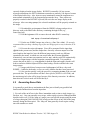
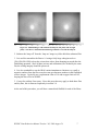
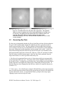
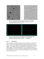
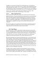
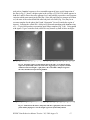
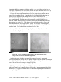
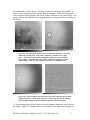
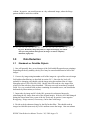
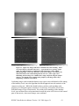
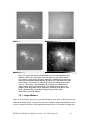
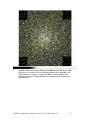
WIYN High-Resolution Infrared Camera
(WHIRC)
Quick Guide to Data Reduction
Dick Joyce
Version 1.03, 2009 August 24
WHIRC Data Reduction Manual Version 1.03, 2009 August 24
1
ACRONYMS AND ABBREVIATIONS:............................................................................................................. 2
1.0
INTRODUCTION.......................................................................................................................... 3
2.0
DATA PREPARATION ................................................................................................................ 3
2.1
2.2
2.3
2.4
2.4.1
2.4.2
2.4.3
3.0
DATA REDUCTION ................................................................................................................... 16
3.1
3.2
3.3
3.3.1
3.3.2
4.0
INITIAL STEPS .............................................................................................................................. 4
GENERATING DOME FLATS .......................................................................................................... 6
GENERATING SKY FLATS ............................................................................................................. 8
ARTIFACT REMOVAL .................................................................................................................... 9
BAD PIXELS.................................................................................................................................. 9
PUPIL GHOST.............................................................................................................................. 11
FRINGES ..................................................................................................................................... 13
STANDARDS OR POINTLIKE OBJECTS ......................................................................................... 16
EXTENDED OBJECTS OR CROWDED FIELDS ................................................................................ 17
COMBINING IMAGES INTO A MOSAIC ......................................................................................... 17
LARGER MOSAICS ...................................................................................................................... 19
DISTORTION CORRECTION.......................................................................................................... 20
APPENDICES .............................................................................................................................. 22
4.1
APPENDIX A – OBSERVATIONAL TEST OF PUPIL GHOST REMOVAL ........................................... 22
Acronyms and Abbreviations:
DHE
FITS
GUI
IAS
IRAF
MOP
PAN
OA
TCS
WHIRC
WIYN
WHOCS
WHOMP
WTTM
Detector Head Electronics (MONSOON system)
Flexible Image Transport System (image standard)
Graphical User Interface
Instrument Adapter System
Image Reduction and Analysis Facility
MONSOON Observing Platform
Pixel Acquisition Node (computer), controls MONSOON
Observing Associate
Telescope Control System
WIYN High Resolution InfraRed Camera
Wisconsin Indiana Yale NOAO (Observatory consortium)
WHIRC Observation Control System
WHIRC Observation Manager and Planner
WIYN Tip/Tilt Module
WHIRC Data Reduction Manual Version 1.03, 2009 August 24
2
WIYN High-Resolution Infrared Camera
(WHIRC) Data Reduction Guide
1.0
Introduction
This document is a quick guide to reducing data taken with the WIYN High Resolution
Infrared Camera (WHIRC). Data reduction is a highly personal process, so one should
keep in mind the procedures described here are biased by the author’s personal
preferences and experience. Many WHIRC users may have their own (possibly superior)
means of reducing data, or use reduction platforms other than IRAF. Suggestions from
the user community will be welcomed.
As noted in the User Manual, the high and variable sky (and telescope) background in the
infrared results in background flux levels on the detector which are often far larger than
the astronomical signals which one is attempting to detect. In addition, the architecture
of infrared arrays is one of independently read out pixels, rather than the charge transfer
utilized with CCDs. Dead or “hot” pixels (with high dark current) therefore show up as
isolated features on infrared images. As with CCDs, observations of a uniformly
illuminated target (flatfields) are used to calibrate the pixel sensitivity function of the
images.
Both the high sky background and the problem of isolated dead or hot pixels are
addressed by taking multiple images of a field, moving the telescope a small distance
between integrations. This technique, referred to as “nodding” or “dithering”, results in
sampling a target at several locations on the array, so the effects of bad pixels can be
minimized. Except in very crowded fields or those with extended structure, one is also
measuring the sky level on every pixel by moving the sources around after each
individual exposure.
2.0
Data Preparation
During a night of observing, one will generally obtain the following types of
observations:
1. Flatfields: We recommend a series of dome flats in each of the filters used, at least 10
each with the lights on and an equal number with the lights off. The latter will serve as
the bias and dark subtraction. One can also generate sky flats using sky frames generated
from the observations and a series of darks of the same integration time. Sky flats may
be more used for reduction in the H and Ks filters, where there is significant thermal
background. One may also use twilight observations for sky flats in the J filter.
Nighttime observations in the narrowband filters will generally not accumulate sufficient
flux for high S/N sky flats, and even twilight flats in the narrowband filters must be
WHIRC Data Reduction Manual Version 1.03, 2009 August 24
3
obtained within a fairly narrow time window. We strongly suggest that observers who
generate sky flats also obtain dome flats as a backup.
2. Science Observations: These can be a series of dithered observations on the source
field (for standards and pointlike sources) or a set of dithered observations on the source
and a set of dithered observations at an off-source sky location.
3. Darks: These are not really required for data reduction, because the process of sky
subtraction will also subtract out any dark current or bias structure. However, a series of
at least 10 short (5 s) darks is a useful diagnostic for evaluating the read noise. If one
generates sky flats, darks at the same integration time are needed.
2.1
Initial Steps
Independent of the reduction platform or individual techniques used for reduction, there
are several steps which should be carried out on all of the data frames prior to any
reduction.
1. Trimming: The raw data frames are 2144 × 2050 pixels in size, with 96 columns of
reference pixels (Fig. 2.1) on the right side and two rows at the top which are presently of
no use and will just make things ugly during the reduction. We suggest trimming these
off of all of the data frames; e.g.,
imcopy *.fits[1:2048,1:2048] *.%fits%tr.fits%
Figure 2.1: Raw Ks band image before (left panel) and after (right panel) trimming.
There is one bad column [97] and row [286] on the detector. The bright spot in the
center of the field is the pupil ghost.
WHIRC Data Reduction Manual Version 1.03, 2009 August 24
4
2. Scaling: If any of the data were taken with Fowler-4 mode, the pixel values must be
normalized by a factor of 4 prior to any linearity correction. The Fowler-4 mode adds all
of the four readouts but does not divide by 4 to avoid possible noise digitization in the
integer output format. So for the Fowler-4 data only:
imarith *.tr.fits / 4. *.tr.fits
will do this in place.
A safer way to do this is to write all of the data to a list, generate a list of the Fowler
samples for all of the data, then divide:
files *.tr.fits > trlist
hselect @trlist fowler yes > flist
imar @trlist / @flist @trlist
3. Linearity correction: As the wells in the array fill up, the gain changes slightly,
resulting in a slightly sublinear response, which is approximately 4% at 38000 ADU. We
have carried out a quadratic fit to the linearity function for 0.7 v bias up to a value of
38000 ADU. By inverting this function, one can derive a linearity correction function so
that the corrected signal S’ is related to the raw signal S by
S′ = S * (A + B*S + C*S2), where
A = 1.0000
B = 1.29 × 10-7
C = 2.506 × 10-11
A′ = 1.0000
B′ = 0.004227
C′ = 0.02691
The IRAF task irlincor is specifically designed to carry out this correction; the coefficients
A′, B′ and C′ above are the irlincor values. It is critical that linearity correction be
performed on the raw data, prior to any sky or dark subtraction, but after any scaling for
multiple Fowler sampling.
Do an epar irlincor and enter the above values for A’, B’, and C’ into the parameter file
(control-D to exit), then
irlincor *.tr.fits *.%tr%lc%.fits
4. At this point you will have three sets of data; you may want to archive the original raw
data somewhere, and the trimmed (.tr.fits) data can be deleted; the
trimmed/scaled/linearized data (.lc.fits) will be used for reduction.
5. The IRAF script wprep.cl, which can be downloaded from the WHIRC web page, will
automatically carry out all of these steps. In addition, it will check the ROTOFF value in
the image header and recalculate the WCS parameters so that the sky coordinates are
WHIRC Data Reduction Manual Version 1.03, 2009 August 24
5
correctly displayed on the image display. ROTOFF is normally 0.0, but at some
telescope orientations, the WIYN instrument rotator has to rotate by 180 degrees because
of the limited cable loop. Also, observers may intentionally rotate the instrument to a
non-cardinal orientation to fit an elongated target onto the array. These offsets are
properly recorded in the ROTOFF keyword, but not in the raw image display at the
telescope. After executing wprep.cl, the celestial coordinates will be properly oriented on
the image.
5.1 Download the script wprep.cl from the WHIRC webpage and put it in a
directory such as the IRAF home directory containing the login.cl file (e.g.,
/home/user/iraf).
5.2 Edit the loginuser.cl file to source the task when IRAF is started up:
task wprep = /home/user/iraf/wprep.cl
5.3 Put the raw WHIRC images into a list (e.g., files *.fits > inlist). We strongly
recommend that you keep a backup copy of the raw images prior to any reduction, to be
safe.
5.4 Execute the script with wprep. You will be prompted for the input data
(@inlist in the present case) and the output data. One may create an output list of the
same length as the input list, but with different image names (such as a different
extension to the name), in which case one would enter the file name (@outlist).
Alternatively, one can enter an extension (such as .wp), and the script will automatically
create new output images with the basename extension appended. It is possible to
execute the task in place (e.g., using @inlist for both the input and output), but this will
lead to confusion with the unprocessed raw data backup, which would have the same
image names.
5.5 Images which have been processed with wprep.cl will have a keyword
WPREP = 1 added to the header, so one can verify whether data have been processed.
5.6 One can also quickly verify the process by comparing imstats of the raw and
processed data. The processed data will have fewer pixels (4194304 vs 4395200), and
the maximum pixel value will be larger because of the linearity correction. In addition,
data taken in Fowler-4 mode will be divided by 4.
2.2
Generating Dome Flats
It is generally a good idea to run imstat on the flats just to identify any possible bad
frames and eliminate them from the input data.
1. For each of the on/off sets in the filters, imcombine each set into a single image (e.g.,
flat.k.on, etc.). One can generally use average, with avsigclip rejection, although median
should work as well. For the ‘lamp on’ images, one can scale the images using the mean
of a large subregion [500:1500,500:1500] to take out the effects of any drift in the lamp
intensity during the observation. The ‘lamp off’ data generally do not require scaling,
since the numbers are small.
WHIRC Data Reduction Manual Version 1.03, 2009 August 24
6
Figure 2.2: Flatfield images at Ks with the flat lamp on (left panel) and off (right
panel). Note there is substantial thermal background flux even with the lamp off.
2. Subtract the ‘lamp off’ from the ‘lamp on’ image to yield a dark-bias subtracted flat.
3. It is useful to normalize the flats to 1.0 using a fairly large subregion such as
[500:1500,500:1500] to keep the science data values from changing too much after the
flatfielding operation. Since all data (science and calibrations) are divided by the same
flat, the scaling integrity should be preserved.
4. It is also worthwhile to use the IRAF routine imreplace to eliminate very small or
negative numbers from the flat so one does not get enormous numbers in the flatfielded
science images. I typically use a replacement value of 1.0 and an upper limit of 0.02,
keeping the lower level at INDEF.
5. Correct for artifacts if necessary. Since this procedure may apply to both dome flats
and sky flats, this is discussed separately in section 2.4.
At the end of this procedure, you will have a normalized flatfield for each of the filters.
WHIRC Data Reduction Manual Version 1.03, 2009 August 24
7
Figure 2.3: Normalized flat for Ks (left panel) and J (right panel). The significant
difference in the two emphasizes the need to obtain dedicated flats in each filter used
for observing. The pupil ghost in the J band is much less prominent, but there is a
noticeable “fingerprint” artifact, probably resulting from a defect in the
antireflection coating on the array. Note that the bad column has been set to a value
of 1.0 by imreplace.
2.3
Generating Sky Flats
We have not yet determined whether sky flats or dome flats are better for data reduction.
Except for the H and Ks bands, though, the nighttime sky flux is generally much too
small to generate high S/N flats. We have generated J band twilight flats by taking a
series of images once the sky level had fallen below the saturation level and combining
them with scaling and a median algorithm, much as is done in the visible. In the Ks
band, thermal background from the telescope and WTTM optics will contribute to the
background and the pupil ghost, whereas the ‘lights on – lights off’ procedure for dome
flats will subtract out this common signal. Since sky flats can be generated from the
target observations, it is safer to get dome flats in any case.
1. Sky flats are best generated from a series of observations which give an appreciable
(several thousand ADU) sky level. This pretty much restricts nighttime observations to
the H and Ks filters. Twilight flats can be taken in the J and (perhaps) narrowband filters,
but the rapid onset of twilight in the infrared leaves limited time for this procedure. H
band sky flats may show fringing from the OH lines, which will complicate the process
(section 2.4.3).
2. Take a series (~ 10) of dark frames (using the OPAQUE filter) at the same integration
time as used for the observations being used to generate the sky flat; this will subtract out
any bias and/or dark current. Average the dark frames, perhaps with average sigma
clipping to prune out maverick pixel values.
WHIRC Data Reduction Manual Version 1.03, 2009 August 24
8
3. Generate a sky image as described in section 3.1. Ideally, one should use a large
number of images (10 or more), at more or less the same airmass, with several thousand
ADU of background.
4. Subtract the averaged dark frame from the sky frame. Normalize and correct for
artifacts as for the dome flats.
2.4
Artifact Removal
WHIRC images contain several types of artifacts, some of which are intrinsic to the
detector, others of which result from multiple reflections within the optics. Correction
for these remains a work in progress, but some techniques are discussed in this section.
Because infrared arrays utilize a unit-cell architecture, the pixels are effectively
independent of each other, unlike those in a CCD.
2.4.1 Bad Pixels
Like all arrays, the detector in WHIRC is not perfect and has several types of cosmetic
imperfections. Some of these can be corrected to a degree during the data reduction.
2.4.1.1
High Dark Current Pixels
These are scattered throughout the array, with certain areas, such as the upper right,
having a higher concentration. These show up as bright pixels, particularly against a low
background such as a dark or narrowband sky. These pixels may also be characterized as
“maverick” pixels, since the signal is not necessarily proportional to the frame time, as a
true dark current would be. The procedure of sky subtraction does seem to remove most
of the elevated signal level, although the noise in these pixels may be higher than in
others. Otherwise, there is no remedy for these artifacts.
2.4.1.2
Dimples
A well-illuminated image such as a flat (Fig 2.3) shows numerous circular artifacts which
appear to be dead pixels. However, closer inspection reveals that these are not dead, but
areas of decreased response which appear to flatfield out reasonably well (Figs. 2.4, 2.5).
The smooth variation evident in a cut through one of the dimples (Fig. 2.5) would make
pixel correction algorithms (such as ‘fixpix’) based on nearest neighbor averaging
problematic.
WHIRC Data Reduction Manual Version 1.03, 2009 August 24
9
Figure 2.4: Expanded subregion of H band image, showing some of the “dimples”
on the detector (left panel). These are not dead pixels and appear to divide out
using a flatfield (right panel) to within 1 – 2 %.
Figure 2.5: Line plot through one of the “dimples” (left panel), illustrating that they
are smoothly varying regions of decreased response. The same dimple after
flatfielding shows that they divide out to within 1 – 2 % (right panel).
2.4.1.3
Dead Pixels
There are a number of unresponsive pixels in the array, including one row [286] and one
column [97] and several clumps which appear to be digs or scratches in the detector
surface. There are various techniques for making bad pixel maps described in the IRAF
literature. One technique which seems to identify most of the dead pixels is to divide two
flatfield images at the same filter and integration times at two different signal levels
(either dome flats at different illumination levels or during a twilight sky flat sequence)
and use imreplace to set the pixels deviating from what should be a narrow distribution to
the “bad pixel value” in the image. Typically bad pixel maps utilize a value of 1 for bad
pixels and 0 for good pixels.
WHIRC Data Reduction Manual Version 1.03, 2009 August 24
10
In addition, one can generate a bad pixel file (which typically has a .pl extension) to
identify specific pixels or regions which are bad. Each line in the file identifies the limits
of the bad region by the values x1, x2, y1, y2; thus the entry 326 349 255 278 identifies
the region between columns 326 and 349 and rows 255 and 278 as bad. This technique is
useful for identifying regions, such as PEDs (section 2.4.1.4) which produce some signal
and may not be completely identified through the flatfield ratio technique. IRAF
reduction tasks will accept either a bad pixel image or file (or both).
2.4.1.4
Photo-emitting Defects
Photo-emitting defects (PEDs) are generally pixels which become shorted during the
hybridization process. They draw significant current during the bias reset and emit light.
PEDs are generally identified during the testing stage by the vendor and “cauterized”
using a laser. This produces a region of limited sensitivity approximately 20 pixels in
diameter, surrounded by a bright annulus. The WHIRC detector has at least two PEDs,
centered near [337:266] and [839:1804]. The first of these appears to still emit some
light and may be responsible for the region of elevated dark current known as the
“palmprint”.
Because these regions are not completely dead, the technique of generating a bad pixel
image by the flatfield ratio technique does not seem to encompass the entire PED, so
using a bad pixel file to identify these regions is good insurance.
2.4.2 Pupil Ghost
As noted in section 2.2, WHIRC images feature a bright region near the center of the
detector. This pupil ghost is a common feature of on-axis refractive optical imagers and
is a result of multiple internal reflections within the optical train. Unlike the MOSAIC
imager pupil ghost, which arises within the corrector and appears as a highly defocused
image of the telescope exit pupil, the WHIRC ghost probably arises within both the
collimator and camera optics and shows up as a broad central peak (Fig 2.3).
Because the pupil ghost arises from the total background flux, it is seen in both sky and
dome flat images. Under reasonably constant sky background conditions, the technique
of sky subtraction will effectively remove the pupil ghost from the science data.
However, the ‘lights on – lights off’ technique for producing dome flats will subtract off
dark current and any common-mode signal, such as thermal emission from the telescope
and WTTM optics in the K band, but not the pupil ghost from the flatfield lights. As a
result, the pupil ghost appears in the reduced flat. Because, this does not represent a true
response peak, using a flatfield with the pupil ghost will result in an artificially reduced
signal level in the central region of the detector. It is therefore necessary to remove this
artifact for accurate calibration of science data.
The IRAF package ‘mscred’, designed for reducing MOSAIC data, has routines for
modeling the pupil ghost and removing it from the data. Unfortunately, the modeling
task works only for ghosts with a central obscuration, as seen with MOSAIC, and is not
effective for the centrally peaked WHIRC ghost. Applying a smoothing function using a
WHIRC Data Reduction Manual Version 1.03, 2009 August 24
11
task such as ‘fmedian’ appears to be a reasonable approach, but a careful inspection of
the flats in Fig. 2.3 shows a bright region in the vicinity of [1250:1250] which appears in
both the J and Ks flats at the same apparent level, and probably represents a true response
variation which must remain in the final flat. Since the pupil ghost is stronger at Ks than
at J, the ratio of the reduced flatfields after bad pixel correction (Fig. 2.6a) may be an
accurate template for the ghost (the J-band “fingerprint” lies well outside the region of
interest). Isolating the central 800 × 800 pixel region and smoothing with fmedian using
a 21 × 21 pixel box produces a promising pupil image template (Fig. 2.6b). Using gauss
with sigma=31 gave a similar result; observers may want to try both of these strategies.
Fig 2.6: (left panel) Ratio of reduced dome flats in Ks and J. Note that the bright
region near [1250:1250] cancels out of the ratio, suggesting it is a response variation
common to both wavelengths. (right panel) The central 800 × 800 pixel region of
the ratio, smoothed to 21 pixels using fmedian.
Fig. 2.7: Dome flat for Ks before (left panel) and after (right panel) removal of bad
pixels and the pupil ghost. Note the bright region near [1250:1250] remains.
WHIRC Data Reduction Manual Version 1.03, 2009 August 24
12
The pupil template can then be used with the task ‘mscred.rmpupil’ to remove the pupil
ghost from the flat (Fig. 2.7). A representative pupil template (whircpupil.fits) can be
downloaded from the WHIRC webpage, although observers may wish to create their
own. The pupil mask (pupmask.pl, also on the webpage) is a four-line file which restricts
the rmpupil task to the central 600 × 600 pixel region. The ‘outtype’ parameter should be
set to ‘sdiff’ since one is subtracting the ghost, and the 5 pixel smoothing for row and
columns seems to be good. The ‘extfit’ parameter should be set to “” (null) because the
WHIRC files are not multi-extension FITS.
Observational tests appear to verify this strategy to be effective in removing the effects of
the pupil ghost (Appendix A).
2.4.3 Fringes
In at least three of the WHIRC filters (Paβ, Paβ45, and H), Newton’s Rings fringes have
been seen in on-sky images. These almost certainly arise from OH emission lines in the
atmosphere and are thus not seen in dome flats (although they may appear in H band sky
flats). The optical configuration within WHIRC which produces these fringes is not
known, but they are textbook Newton’s Rings centered at the same location on the
detector in all filters where they are seen. The Paβ and Paβ45 fringes appear
monochromatic, whereas the H band fringes show amplitude modulation suggesting
several wavelengths are contributing (most likely the strong OH Q-branch lines in the H
band).
Unfortunately, unlike the pupil ghost, the fringe patterns differ for each filter in both
spacing (wavelength-dependent) and phase. In addition, fringe patterns seen in a given
filter appear to vary slightly in phase from one night to another. Therefore, one cannot
use a generic template to attempt removal of the fringe pattern, but must use the data
from the same night.
Because the strength of the OH lines varies during the night, fringes may not be seen in
the sky frame (see section 3.1) for any given target, but they may very well appear in a
“supersky” generated from all of the observations during a given night. This is often the
case in the H band; in the Paβ and Paβ45 filters, the fringes will almost always be
prominent since the continuum sky background is negligible and science exposures tend
to be long.
The MOSAIC reduction task mscred.rmfringe appears to do a credible job of removing
these fringes from the sky frame. As with the rmpupil task, one needs a template of the
pattern, which will then be amplitude fitted to the fringes in the data and subtracted.
Since a generic template cannot be used, one must generate the template from the science
observations. Refer to sections 3.1 and 3.2 following, since the fringe removal will be
carried out during these steps of the data reduction. It is logical to apply the fringe
removal to the sky-subtracted data, since the sky subtraction may remove most, if not all,
of the fringing, and it is generally preferable to reduce any artifacts to the extent possible
before applying additional reduction steps.
WHIRC Data Reduction Manual Version 1.03, 2009 August 24
13
Generating the fringe template is similar to making a sky flat (without the flat), so one
will require, in addition to the science data, a dome flat in the same filter and a series of
darks taken at the same integration time as the science data.
1. Create a sky image using imcombine on all of the images in a given filter on each
target field with median filtering. Since the sky level will probably be changing, one
should scale the image using the median value of a large subregion such as
[500:1500,500:1500]. Ideally, this will result in a sky image from which all of the stars
have been eliminated. This may not work in extremely crowded fields. For very
crowded fields or those containing an extended source, one should take dedicated sky
observations (see section 3.1). If one observed several fields through the filter at the
same integration time, one may generate a “master” sky image by imcombining all of
these images; this may enhance the fringe visibility as well as increasing the S/N of the
resulting frame. The result will look something like Fig. 2.8a.
2. Average the dark frames (as in making a sky flat, section 2.3) and subtract from the
average sky frame (Fig. 2.8b).
Figure 2.8: Average of sky images in the Paβ filter (left panel), showing evident
fringes. After subtraction of dark frame (right panel).
3. At this point most of the dark current will be removed, except for occasional
mavericks, but the frame still has the low spatial frequency structure and the central pupil
ghost. Dividing by the dome flat and running fixpix with the bad pixel mask will remove
most of the structure and clean up the image (Fig. 2.9a).
4. The fringe template for rmfringe has (ideally) a minimum value near zero, so one can
at this point subtract off a constant value to achieve this. Running fmedian with a fairly
small box (3 × 3) appears to enhance the S/N without affecting the spatial resolution of
the template (Fig. 2.9b).
WHIRC Data Reduction Manual Version 1.03, 2009 August 24
14
For comparison, we show in Fig. 2.10 fringe templates for the Paβ45 and H filters, to
show the need for filter and time-specific fringe information. While the Paβ45 pattern
seems similar to the Paβ pattern, one can see a phase difference in the central fringe. The
fringe visibility in the H band varies, suggesting that several emission lines contribute to
the fringes.
Figure 2.9: (left panel) Paβ sky image from Fig. 2.8b after dividing by a dome flat
and cleaning up bad pixels. Some of the “palmprint” can still be seen. (right
panel): After subtracting the background and smoothing, one has an adequate
fringe template. The white blobs are probably artifacts from bright stars in the
original images which were not completely removed by the median filtering.
Figure 2.10: Fringe templates derived from sky data in the Paβ45 (left panel) and H
(right panel) filters. Note the phase shift in the central fringe between the Paβ (Fig.
2.9b) and Paβ45 templates and the amplitude modulation in the H template.
5. Using the appropriate fringe template, the task rmfringe can then be used to remove
the fringes. Figure 2.11 illustrates this for a H band sky on a night where fringing was
WHIRC Data Reduction Manual Version 1.03, 2009 August 24
15
evident. In practice, one would operate on a sky-subtracted image, where the fringe
pattern should be much less evident.
Fig. 2.11: H band sky image (left panel) on a night when fringing was evident.
After processing with the rmfringe task, the fringes are almost completely
eliminated (right panel).
3.0
3.1
Data Reduction
Standards or Pointlike Objects
1. One will generally have several images of the field with different telescope pointings.
Depending on the sky stability, the sky level may be somewhat different in each of the
images.
2. Create a sky image using imcombe on all of the images in a given filter on each target
field with median filtering, as described in section 2.4.3. Since the sky level will
probably be changing, one should scale the image using the median value of a large
subregion such as [500:1500,500:1500]. Ideally, this will result in a sky image from
which all of the stars have been eliminated. This may not work in extremely crowded
fields. For very crowded fields or those containing an extended source, one should take
dedicated sky observations (see below).
3. Inspect the sky image and if it looks OK, generate sky-subtracted images by
subtracting the sky image from each of the original images. If the sky level had changed
during the observation series, some of the sky levels may be positive, some negative.
Keep going. Fringe removal, if necessary, can be done at this stage.
4. Divide each sky-subtracted image by the flat for that filter. This should result in
images in which the (non-zero) sky level is uniform across the image. One can subtract
WHIRC Data Reduction Manual Version 1.03, 2009 August 24
16
this offset out by measuring the median level of the image and subtracting that number.
If one is doing aperture photometry, the sky level should be automatically subtracted
during that process.
5. One may analyze the results from each image separately or combine them, using
upsqiid or other custom routines. If making a large mosaic of images, distortion
correction may be needed to ensure good overlap of the stars different images (section
3.3.2).
3.2
Extended Objects or Crowded Fields
1. As with the pointlike fields, one should have several dithered images of the science
field, but also a set of dithered images taken at a not too distant “sky” position relatively
devoid of stars.
2. Combine the off-target sky images as above using median filtering.
3. Subtract the sky image from each of the target images to yield the sky-subtracted
image.
4. Flatfield the sky-subtracted images as above.
5. One may analyze the results from each image separately or combine them, using
upsqiid or other custom routines.
3.3
Combining Images into a Mosaic
For IRAF users, the upsqiid package written by Mike Merrill can be used to align and
combine the images into a single image. This is primarily useful for deep imaging, where
one is observing the same field with relatively small dither amplitudes, since it relies on
locating star(s) common to all images for alignment. Although this package was written
primarily for data from the 4-color imager SQIID, the routines for aligning and
combining individual images into a mosaic are applicable for WHIRC images. A
description of the upsqiid package, as well as instructions for downloading the package
into IRAF, can be found at http://www.noao.edu/kpno/sqiid/upsqiidpkg.html.
Three basic tasks which have been found useful for combining images are:
xyget – Find common stars in the images and create a registration database
zget – Find intensity offsets from overlap regions in the registration database
nircombine – Combine the registration database into a composite image
For mosaics involving large dither amplitudes, distortion correction may be advisable to
ensure proper overlap of the star images in different fields. See section 3.3.2 for details.
WHIRC Data Reduction Manual Version 1.03, 2009 August 24
17
Figure 3.1: (upper left) Image of the NGC 7790 field at Ks, after trimming. This is
one of nine images of the field, taken in a 3 × 3 grid with 50 arcsec spacing. (upper
right) Sky image obtained by combining the nine input images with a median
filtering algorithm. (lower left) Difference of the top two images. Note that the sky
subtraction reduces the residual background to near zero. (lower right) After
flatfielding, the nine images are combined into a single composite using the upsqiid
package. Note that the noise is higher in the periphery of the image where only a
single image contributes to the mosaic.
Combining images with extended nebulosity may require some individualized fine tuning
of the intensity levels, since the algorithm used in the zget task uses the statistics of the
common overlap area. While this should in theory produce good matching at the
periphery of overlapped regions, sometimes it is necessary to tweak the levels in the
individual images to get a better match. Even with perfect matching of the intensity
levels, one can detect the overlap transitions because the noise will be lower in the central
parts of the mosaic, where more images were combined.
WHIRC Data Reduction Manual Version 1.03, 2009 August 24
18
Figure 3.2: (upper left) Image of the M42 field in the narrowband H2 filter, after
trimming. This is one of five images of the field, taken in a plus pattern with 50
arcsec spacing. (upper right) Sky image obtained by combining the five images of a
nearby sparse field with a median filtering algorithm. (lower left) Difference of the
top two images. Note that the sky subtraction reduces the residual background to
near zero. (lower right) After flatfielding, the five images are combined into a
single composite using the upsqiid package. Note that the noise is higher in the
periphery of the image where only a single image contributes to the mosaic. This
image is displayed using a logarithmic scaling to bring out faint details.
Observations courtesy M. Meixner.
3.3.1 Larger Mosaics
Maps covering a larger area may be generated using the more generic IRAF tasks in the
noao.imred.irred package. In particular, the tasks irmosaic, iralign and irmatch2d can be
used in a manner analogous to the upsqiid tasks noted above, except that the iralign task
WHIRC Data Reduction Manual Version 1.03, 2009 August 24
19
works in the overlap region between two adjacent images only. The only precondition is
that the input images have some spatial overlap with their neighbors.
The irmosaic task combines the input images into a single N x M mosaic, in the same
geometry that they were taken on the sky. One then uses iralign to identify pairs of stars
common to adjacent images until all nearest neighbors have been matched. The
separations between these stars in the mosaic image is written to a database. The
irmatch2d task shifts the images in the original mosaic to that the adjacent stars match up,
creating a single composite image.
NOTE: Because WHIRC is designed to exploit the good seeing at WIYN, particularly
once WTTM is operational, it is expected that it will be used mostly for deep mapping of
relatively small areas. Other instruments, such as NEWFIRM, are better suited to widefield surveys.
3.3.2 Distortion Correction
Because WTTM utilizes off-axis reflective optics, the plate scale is different in the x and
y coordinates on the detector (0.0969 and 0.1002 arcsec/pixel, respectively). In addition,
there is a small amount of field distortion at the input to WHIRC. The distortion is
asymmetric (keystone) and is less than 1%. The additional distortion from WHIRC is
very small and is negligibly dependent on wavelength.
During the design of WHIRC, the entire optical system (WIYN telescope, WTTM, and
WHIRC) was modeled using Zemax, and optical distortion maps were generated in the J,
H, and Ks filters. These files were used as input to the IRAF routine geomap to generate
third-order polynomial fits with an rms error ~ 0.1 pixel. The files
whirc.distort.<filter>.txt and whirc.distort.<filter>.db produced by geomap can be
downloaded from the WHIRC webpage and used in the routine geotran to produce
distortion-corrected images which can then be combined into a large mosaic with good
registration to the edges of the field (Fig. 3.3). The chromatic effects on distortion are
extremely small, so the distortion files are almost identical.
NOTE: Because geotran remaps each pixel slightly, one should carry out the distortion
correction on images which have already been processed by sky subtraction and
flatfielding. We have not investigated the effects of distortion correction on surface
brightness measurements of extended sources. The geotran routine should preserve flux
when the ‘fluxconserve’ flag is set to ‘yes’. Until we gain more practical experience in
quantitative evaluation, we suggest that observers be conservative, or at least cognizant,
of the potential effects of distortion correction on photometry. Programs utilizing deep
imaging of a small field using small dither amplitudes probably do not require correction.
Imaging over a more extended field, even with small dither amplitudes, may benefit from
distortion correction when using PSF-fitting photometry.
WHIRC Data Reduction Manual Version 1.03, 2009 August 24
20
Figure 3.3: Mosaic of five images of the M13 field in the H band. The images, offset
by 50 arcsec in a + pattern, were corrected using geotran prior to mosaicking. The
2MASS point source catalog is overlaid on the field. Except for multiple sources
mistakenly cataloged as a single 2MASS source, the positional fit is excellent to the
edge of the field.
WHIRC Data Reduction Manual Version 1.03, 2009 August 24
21
4.0
4.1
Appendices
Appendix A – Observational Test of Pupil Ghost Removal
On the (apparently) photometric night of 9 July 2009 UT we tested the pupil ghost
removal technique described in section 2.4.2 by sampling a region approximately 80
arcsec square centered on the array. An arbitrary star (Ks ~ 11) on the outskirts of M13
was measured using four 5 × 5 dither sequences of amplitude 10 arcsec, each of which
was offset by 18 arcsec in both RA and DEC from the center of the array in the four
possible directions. This gave high spatial sampling of the area around the center of the
pupil ghost (approximately [1032:1002] on the array). The experiment was done in the
Ks filter where the pupil ghost is most pronounced. The focus was checked between each
of the four sequences to ensure that the image quality did not drift significantly during the
experiment; seeing was modest (0.6 – 0.7 arcsec).
Data reduction was done in the standard way. The 100 frames were median combined to
generate a sky frame, which was subtracted from each of the input frames to yield the
sky-subtracted images.
Good quality dome flats in the J and Ks filters were obtained using the standard “lights
on, lights off” technique, subtracted and then corrected for bad pixels using the fixpix task
and the WHIRC bad pixel mask. The flats were normalized using regions
[400:600,400:1600] and [1400:1600,400:1600], which avoids the pupil ghost area, and
any other pixels of value < 0.02 were set to 1.0 to avoid arithmetic blowup in the
flattened images. These flats, which contain the pupil ghost, are referred to as the
uncorrected flats.
The template for removal of the pupil ghost was generated as follows:
•
•
•
•
•
The normalized Ks and J band flats were ratioed to give a flat ratio image
A new 2048 × 2048 image with pixel value = 1.0 was generated with mkimage
The central 800 × 800 of the flat ratio image centered on the pupil ghost
[625:1424,601:1400] was copied into the new image
The image was smoothed using the gauss task with sigma = 31
Subtract 1.0 from the result to yield the pupil ghost template image
The uncorrected flats were run through the rmpupil task using the pupil ghost template
image as the ‘pupil’, and the pupil mask file pupmask.pl as the ‘pupilmask’ to restrict the
procedure to the central 600 pixels [725:1324,725:1324]. The parameter ‘outtype’ was
set to “sdiff”, since one is subtracting the ghost, and the column and line smoothing were
set to 20. The resulting flats were the “nopupil” flats.
WHIRC Data Reduction Manual Version 1.03, 2009 August 24
22
The sky subtracted images were flattened with both the uncorrected and nopupil flats,
yielding three datasets of 100 images each:
•
•
•
Sky-subtracted, unflattened images
Uncorrected flattened images
Pupil corrected flattened images
The selected star was measured using apphot with a fairly large (4 arcsec diameter)
aperture to minimize the effects of seeing or focus drifts for all three datasets. The X and
Y coordinates were translated to radial distance from the pupil ghost center at
[1032:1002]; this was used as the abscissa for plotting the measured signal levels (Fig.
4.1).
The figure illustrates that the uncorrected flat does have the anticipated effect of reducing
the point to point scatter in the measured flux, but introduces a very significant (0.15
mag) systematic artifact as a result of the pupil ghost. The additional illumination in the
ghost results in signal levels which are too faint. The bottom panel of the figure
demonstrates that the pupil removal procedure has effectively eliminated this artifact.
The rms scatter in the pupil-corrected flattened images (0.024 mag) is significantly less
than that in the unflattened images (0.035 mag), but is still larger than earlier tests with a
9 x 9 raster of a standard star field had yielded. The current experiment of measuring 100
positions over a 40 minute time frame does make assumptions about photometric stability
over this time frame during a time of year not known for clear weather. A plot of the data
with time (Fig. 4.2) does appear to show some systematic variation, as well as a slope
which is probably a result of atmospheric extinction (Δz ~ 0.2) during the sequence. The
p-p scatter around a low-order fit is ~ 0.05 – 0.06 mag, equivalent to an rms ~ 0.015 mag.
An alternative approach is to image a field which is sufficiently crowded to spatially
sample the area within and around the pupil ghost, as this would not be sensitive to
changes in sky transparency. Unfortunately, real-life stellar fields of sufficient density
are usually confusion limited with many fainter sources contributing a background which
calls into question the photometric reliability of relatively coarse resolution surveys such
as 2MASS.
WHIRC Data Reduction Manual Version 1.03, 2009 August 24
23
Figure 4.1: Plots of the magnitude of a Ks ~ 11 star measured in a 4 arcsec aperture
using the IRAF task apphot over a 10 x 10 raster centered on the WHIRC pupil
ghost. The magnitude scale is not calibrated to a photometric standard. The same
dataset is plotted for the sky-subtracted, unflattened data (top panel), data flattened
with no correction for the pupil ghost (middle panel), and data flattened with
correction for the pupil ghost (bottom panel).
WHIRC Data Reduction Manual Version 1.03, 2009 August 24
24
Figure 4.2: The pupil-corrected flattened data from the lower panel of Fig. 4.1, but
plotted as a function of time, in the order the data were obtained. The line is a
linear fit to the data and probably represents atmospheric extinction, since the
airmass increased over the span of the observations by approximately 0.20.
WHIRC Data Reduction Manual Version 1.03, 2009 August 24
25