Download Saturn User Manual

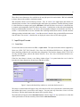
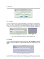
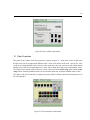
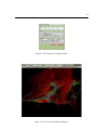
Saturn User Manual
Rubén Cárdenes
29th January 2010
Image Processing Laboratory, University of Valladolid
Abstract
Saturn is a software package for DTI processing and visualization, provided with a graphic user interface (GUI). This document describes the steps required to load DTI data, and to operate with them:
compute and visualize scalar magnitudes derived from DTI data, perform tractography, perform automatic fiber clustering, perform glyph rendering, compute measures over regions of interest (ROIs) and
along fiber tracts, and edit fibers and ROIs.
Contents
2
Contents
1
Introduction
2
Input/Output Formats
2.1 Scalar Data . . .
2.2 Tensor Data . . .
2.3 DWI Data . . . .
2.4 Model Data . . .
3
.
.
.
.
.
.
.
.
.
.
.
.
.
.
.
.
.
.
.
.
.
.
.
.
.
.
.
.
.
.
.
.
.
.
.
.
.
.
.
.
.
.
.
.
.
.
.
.
.
.
.
.
.
.
.
.
.
.
.
.
.
.
.
.
.
.
.
.
.
.
.
.
.
.
.
.
.
.
.
.
.
.
.
.
.
.
.
.
.
.
.
.
.
.
.
.
.
.
.
.
.
.
.
.
.
.
.
.
.
.
.
.
.
.
.
.
.
.
.
.
.
.
.
.
.
.
.
.
.
.
.
.
.
.
.
.
.
.
.
.
.
.
.
.
.
.
.
.
.
.
.
.
.
.
.
.
.
.
.
.
4
4
5
5
6
3
Visualization Windows
7
3.1 2D Windows . . . . . . . . . . . . . . . . . . . . . . . . . . . . . . . . . . . . . . . . . . 7
3.2 3D Window . . . . . . . . . . . . . . . . . . . . . . . . . . . . . . . . . . . . . . . . . . . 10
4
Scalar Magnitudes
12
5
Scalar isosurfaces
13
6
Tractography
6.1 Color options . . . . . .
6.2 ROIs Edition . . . . . .
6.3 Normal Tractography . .
6.4 Brute Force Tractography
6.5 Logic Operations . . . .
.
.
.
.
.
.
.
.
.
.
.
.
.
.
.
.
.
.
.
.
.
.
.
.
.
.
.
.
.
.
.
.
.
.
.
.
.
.
.
.
.
.
.
.
.
.
.
.
.
.
.
.
.
.
.
.
.
.
.
.
.
.
.
.
.
.
.
.
.
.
.
.
.
.
.
.
.
.
.
.
.
.
.
.
.
.
.
.
.
.
.
.
.
.
.
.
.
.
.
.
.
.
.
.
.
.
.
.
.
.
.
.
.
.
.
.
.
.
.
.
.
.
.
.
.
.
.
.
.
.
.
.
.
.
.
.
.
.
.
.
.
.
.
.
.
.
.
.
.
.
.
.
.
.
.
.
.
.
.
.
.
.
.
.
.
.
.
.
.
.
.
.
.
.
.
.
.
.
.
.
14
14
15
15
15
16
7
Automatic Fiber Clustering
17
8
Measures
19
8.1 ROIs Measures . . . . . . . . . . . . . . . . . . . . . . . . . . . . . . . . . . . . . . . . . 19
8.2 Fibers Measures . . . . . . . . . . . . . . . . . . . . . . . . . . . . . . . . . . . . . . . . . 19
9
Fiber Edition
21
10 Fiber Properties
22
11 Glyphs
23
3
1
Introduction
This document describes the features implemented in the DTI processing and visualization tool called Saturn, at user level. The general features of this application are:
• Object Oriented.
• Multi-platform.
• Efficiency.
• Easy to handle for non expert users.
• Wide Input/Output file format support.
• Documentation
• On line availability.
The general view of the Saturn graphic user interface (GUI) appears in figure 1. This GUI is divided in two
main panels: the control panel, on the left side of the main window and the visualization panel on the right
side. The control panel is divided in two panels: the data panels, where the data loaded and/or created will
be listed, and the options panel where the parameters and procedures can be accessed. There exist also a
menu bar at the top of the main window, that give access to the major part of the features included. Finally
a status bar is placed below the visualization panel, that indicates the percentage of time taken for some
processes.
Figure 1: General view of the Saturn GUI
4
Three direct access buttons are also available in the top right part of the main window: 3D, 3+1 and 4x2D,
to choose between the available visualization modes.
This document consists on the following sections. First, in section 2 the input/output data formats are
described, then in section 3 the visualization modes and features are explained. Then the following sections
it is described how to compute and visualize DTI data in 2D and 3D modes. In section 4 it is described how
to compute scalar magnitudes from DTI while in the section 5 explains how to show this scalar magnitudes
images as tridimensional isosurfaces. In section 6 the tractography techniques are described at user level. In
section 7 it is described how to use the automatic fiber clustering method, then section 9 describes the fiber
edition procedures included and section 10, and then section 8 describes how to obtain different measures
from DTI data. The section 11 describes how to display the tensor values of DTI data as glyphs.
2
2.1
Input/Output Formats
Scalar Data
To load scalar data use the menu item: File -> Open Scalar. The input scalar data formats supported by
Saturn are: JPEG, TIFF, PNG, MetaFile, Kretz, Raw data, DICOM and DICOM series. In figure 2a it is
shown the dialog window for the scalar data entry information. The first three formats (JPEG, TIFF, PNG)
can only load 2D images, whereas the formats MetaFile, Kretz, Raw data, DICOM and DICOM series,
support 2D or 3D data.
If the Raw data format is chosen, a new dialog window (figure 3) is opened where the user is asked to
introduce the image dimensions, the pixel type and the byte order.
(a)
(b)
Figure 2: Input scalar data dialog window (a), and scalar data browser (b).
The image or volume loaded will appear in any of the three first 2D viewers placed in the visualization panel
(the bottom right viewer is reserved for color images). You can select any of the three viewers to see the
new images, with the check buttons that appears in the open file dialog.
The loaded data will appear in the scalar data browser, shown in figure 2b. Any operation over scalar data
will be performed over the data currently selected in the scalar data browser.
2.2
Tensor Data
5
Figure 3: Input scalar data dialog window
2.2
Tensor Data
To load tensor data use the menu item: File -> Open Tensor. The input tensor data format supported by
Saturn are: vtk, and nrrd. The input dialog window shown in figure 4a will appear to choose the file name
and type. The tensor data loaded will be listed in the tensor data browser (see figure 4b) and additionally, a
FA volume will be computed and visualized in the first 2D viewer and stored in the scalar data browser (2).
(a)
(b)
Figure 4: Input tensor data dialog window (a), and tensor data browser (b).
2.3
DWI Data
To load a set of Diffusion Weighted Images (DWI) use the menu item: File -> Open DWI. The data format
supported in this case is DICOM series. The DWI input dialog window, as the one shown in figure 5, will
appear.
Figure 5: Input DWI data dialog window
Use the explore button to go to the directory where the DWI series is stored and select one of the images.
Once the series is selected, two different operations are supported: Open, it just open the volume and store it
2.4
Model Data
6
internally in a DWI object data. The Open and Process where the DWI files are filtered, masked, the tensor
is estimated and stored in the tensor data browser (4b), and the FA is computed, shown in the first viewer
and stored in the scalar data browser (2). Notice that these set of procedures are computationally expensive,
taking from 1 to 10 minutes depending on the machine processor, load of the system and operating system
used.
2.4
Model Data
To load model data (fiber tracts) use the menu item: File -> Open Model. The input model data format
supported by Saturn is vtk. The loaded data will appear in the model data browser (see figure 6). Any
operation over model data will be performed over the data currently selected in that browser. To save model
data go to File -> Save Model and choose a file name for the model. The model saved will be the one
selected in the browser.
Figure 6: Model data browser.
7
3
3.1
Visualization Windows
2D Windows
Once the data is loaded, it appears in one of 2D viewers of the visualization panel, as the one shown in figure
7a. These viewers always show 2D images, but they are able to show orthogonal cuts of the volume loaded
(pressing the buttons 0,1,2 when the cursor is over them or using the selection box at the bottom right of
each viewer). There is also a slider at the bottom of each viewer that allows to change the slice shown in
volume data.
(a)
(b)
Figure 7: 2D Viewer (a) and independent window viewer (b).
There exist also several buttons in the top of each viewer. From left to right these buttons are:
• Show details button. Shows image details overlaid in the viewer.
• Show value button. Shows cursor position and image value at that position, overlaid in the viewer.
• Flip vertically. Flip the image vertically.
• Flip horizontally. Flip the image horizontally.
• Show preferences. Show the preferences panel.
• Zoom in. Zoom in the image.
• Zoom out. Zoom out the image.
• Translate right. Translate right the image if zoom in is on.
• Translate left. Translate left the image if zoom in is on.
• Translate up. Translate down the image if zoom in is on.
• Translate down. Translate down the image if zoom in is on.
• Show in Color. Show the image in RGB color maps.
• Show in Gray. Show the image in grayscale color maps.
3.1
2D Windows
8
• Show anatomical labels. Shows anatomical labels (A,P,R,L,I,S), overlaid in the viewer.
• Expand the viewer. Maximize the viewer to the maximum size of the visualization panel.
The scalar data can be shown in any of the viewers using the View button placed in the scalar data panel. In
figure 8 we show an example of this. Once pressed the View button, the scalar data currently selected, in
this case Volume FA, is shown in the selected viewer (upper right viewer). To select a viewer just check the
check-button placed at the bottom right of each viewer, as shown also in figure 8.
Figure 8: Scalar view selection
Additionally the scalar data can be also shown in an independent window as the one shown in figure 7b. To
show that select the scalar data to visualize and click in View Out button.
Each 2D viewer has also a set of options, accessible from the keyboard. The key-feature correspondence is
outlined in the table 1.
Some of the features are also available from the preferences panel shown in figure 9. This panel is accessible
from the menu item Saturn-> Preferences or from the P button of each viewer. From this panel, some
features can be controlled as for instance, flip the image in any direction, transpose the image, zoom in and
out, display the cursor cross, the cursor value and the image details.
A set of controls present of this panel are designed to control an important feature available in the viewers,
which are the image modes. The image can be shown in two different image modes: grayscale image mode
and color image mode. The Image mode box changes the different color maps available in the grayscale
image mode, which are VAL (intensity), INV (inverse intensity), LOG (logarithmic scale), DX (derivate
respect to x), DY (derivate respect to x), DZ (derivate respect to z), BLEND (mix with the with the previous
and following slice), and MIP (projection of all the values). The Color mode box box changes the different
color maps available for the color image mode, which are FA, ROIs, Heat and Discrete.
3.1
2D Windows
0
1
2
<,
<,
r
h
x
y
z
qw
e
as
d
+=
-_
imjk
t
A
C
I
T
P
D
O
p
l
9
See cuts in the x axis
See cuts in the y axis
See cuts in the z axis (by default)
See the following slice
See the previous slice
reset all the options
help (this summary)
Flip x axis
Flip y axis
Flip z axis
Diminishes, increases the top limit of the window in intensity
alternates the values of the top limit windows in intensity between
clipping and setting-to-black
Diminishes, increases the lower limit of the window in intensity
alternates the values of the lower limit windows in intensity between
clipping and setting-to-black
Zoom-in a factor 2
Zoom-out a factor 2
Moves the image int he directions up, down, left, and right.
Transposes the axis of the cut showed
See axis labels: P=posterior, L=left, S=superior
See crosses where the cursor is
See image values where the cursor was last clicked
Show or hide the clicked points
Change the coordinates between index and physical units
See image details superposed
See a superposed color
Save to a file the clicked points
Change the the screen data showing way
Ways change cyclically in the following views:
Intensity, Inverse, Log, Derivative respect to x, y and z,
mix with the with the previous and following slice, and MIP
Table 1: Available options in the 2D viewers
Finally, the sliders of this panel controls the intensity in the grayscale image mode (gray sliders), and the
color range in the color image mode (green sliders).
3.2
3D Window
10
Figure 9: Preferences panel to control the 2D viewers.
3.2
3D Window
The 3D viewer for the visualization of scenes is shown in figure 10. This viewer can be shown using the 3D
button at the top right of the main window.
The features supported by the 3D viewer are:
• Center: Center the scene in the viewer.
• Orthogonal planes view: using the coronal, sagittal and axial check buttons. The data shown in these
planes will be the scalar data selected in the scalar data browser (2). Planes slide: using the coronal,
sagittal and axial sliders or using the middle button of the mouse and dragging. The cursor should be
at the zone of the 2D outside the blue lines, (interior zone of the plane).
• Oblique planes view: using the middle button of the mouse and dragging. The mouse must be located
in the zone of the plane marked by the blue lines (see figure 11a).
• Color image mode: Change the to image mode in the planes to RGB mode, with the Color button.
• Gray image mode: Change the to image mode in the planes to grayscale mode, with the Gray button.
• Planes intensity change: Using the right button of the mouse and dragging.
• Planes value view: Left clicking with the mouse a red cross in the plane appears as well as the
position value and the value (see figure 11b).
• Plane Opacity: Change the opacity shown in the 2D planes, using the Opacity slider.
• Zoom in and out: it can be using the + and - buttons, and also by right-clicking and moving the
mouse.
• Rotate scene: Using the mouse left button and dragging.
• Translate the scene: Pressing the SHIFT button on the keyboard with the mouse left button and
dragging.
3.2
3D Window
11
Figure 10: 3D Viewer.
• Spin the scene: Pressing the CTRL button on the keyboard with the mouse left button and dragging.
• Pointing at the scene: Using the mouse middle button and dragging.
• Predefined views: using the A,P,L,R,I and S buttons.
12
(a)
(b)
Figure 11: 3D viewer with oblique plane (a) and cursor value view (b).
4
Scalar Magnitudes
The scalar magnitudes that can be derived from DTI data available in Saturn, are controlled from the panel
shown in figure 12. These are: Fractional Anisotropy (FA), Relative Anisotropy (RA), Mean Diffusivity
(MD), Color by Orientation, Geometric Coefficients, linear (Cl ), planar (Cp ), and spherical (Cs ), eigenvalues
ordered from high to low: major (Eig 1), middle (Eig 2) and minor (Eig 3), and tensor components: Dxx ,
Dxy , Dxz , Dyy , Dyz , and Dzz . Representing the tensor D as a positive semidefinite 3x3 matrix, there exist only
six independent components:


Dxx Dxy Dxz
D = Dxy Dyy Dyz 
Dxz Dyz Dzz
(1)
There is a button for each scalar magnitude. After a button is pressed the corresponding scalar data is
computed and stored in the scalar data browser (2), except for the color by orientation. In that case the
resulting RGB image is shown in the fourth viewer (bottom right 2D viewer) and no scalar magnitude is
stored. The color codes in this images, by convention is: red for RL direction, green for AP direction, and
blue for IS direction.
A screenshot with some scalar magnitudes computed and visualized is the shown in figure 13.
13
Figure 12: Scalar magnitudes control panel
Figure 13: Scalar magnitudes, FA, MD, Cp and color by orientation.
5
Scalar isosurfaces
The scalar magnitudes of a DTI data can also be visualized by tridimensional surfaces. This surfaces represents points of a constant scalar value within the scene. The user must define the limits and values that wants
to display. The control panel for isosurfaces is shown in figure 14; user can access on this panel pressing
the Do Model button placed under the scalar data browser. The input data is taken from the scalar data
selected in the scalar data browser and shown in the Input1 selector; the name of the resultant output is
shown in the Output selector. The Full Model slider controls the accuracy of the model (a one hundred
percent value will display a full model while a zero percent value will display a simpler one); the Range
min and Range Max sliders control the range of scalar values of the data that will be used for surface calculation. The num counter controls the number of surfaces created for the model within the selected range.
The Opacity slider controls the transparency of the model selected in the model data browser. The Apply
button finally creates the isosurfaces with the selected parameters.
14
(a)
(b)
Figure 14: Scalar isosurfaces panel (a) and Scalar isosurfaces viewer (b).
6
Tractography
In figure 15 the features and parameters related to tractography are available. The panel is divided into four
sections: Color, Parameters, ROIs and Execution. In the following all these sections are explained in
detail. The upper buttons marked as Auto and Measures allows to access quickly to the Automatic fiber
Clustering and the Measures sections.
Figure 15: Tractography control panel
6.1
Color options
The first section of the panel controls the color code used for the fibers to be computed. There are six
possibilities:
6.2
ROIs Edition
15
1. FA. Color by FA: red colors are assigned to points with low FA, blue to points with large FA and
green to points with intermediate FA values. By default the color range is assigned from 0 to 0.8.
2. Size: Color by fiber size: red colors are assigned to short fibers, blue to large fibers and green to
intermediate size fibers. The scale is done independently for each fiber tract computation.
3. RGB. The fiber is colored depending on the seed label or class.
4. Distance. Color by distance of the points to the nearest seed in each fiber.
5. Major Eig. Color by the major eigenvalue: red colors are assigned to points with low first eigenvalue,
blue to points with large first eigenvalue and green to points with intermediate first eigenvalue. By
default the color range is assigned from 0 to 0.8.
6. Predefined color. The fibers will be colored with one of the predefined colors: (skin, bone, gray, red,
green, blue and sea).
6.2
ROIs Edition
First, it it is necessary in all the tractography modes to draw or select a region of interest (ROI). This is done
in the 2D viewers by left click with the mouse over it. The user can add a ROI with a predefined radius and
label, that can be changed in the ROIs section of the Tractography panel. By dragging the mouse while
left clicking it is possible to draw ROIs in any of the orientations (axial, sagittal or coronal), and in any slice.
To remove all the ROIs drawn use the clear or to erase part of the ROIs, choose class 0 and draw using the
mouse. It is also possible to change the opacity of the ROIs using the opacity slider. To load ROIs from a
file use the File -> Load ROIs menu item. It is also possible to save the ROIs using the File -> Save ROIs
menu item.
6.3
Normal Tractography
The most simple tractography procedure can be done using the Tractography button. The result will be the
set of fibers that start from the ROIs drawn. There exist two stopping criteria for the algorithm: the minimum FA (the fiber path computation is stopped if the FA is lower that a given threshold), and a maximum
angle (the fiber path computation is stopped if the curvature angle is higher that a given threshold). Those
thresholds can be set by the user using the FA threshold and Curv Threshold sliders. Additionally the step
length, an internal parameter that controls the tractography integration procedure can be set by the user. The
default value is proven to work properly for most of the cases. The last parameter is the radius of the tube
drawn to represent the fibers computed.
6.4
Brute Force Tractography
Using the Brute Force button, the brute force tractography is computed using all the voxels over the FA
threshold as seeds. The result of this operation is not possible to be shown due to the high amount of data
obtained typically by this operation. In order to show a set of fibers computed with the brute force algorithm,
the select fibers button is needed. After clicking that button, the fibers that pass through the ROIs drawn are
visualized and stored in the model data browser (6).
6.5
Logic Operations
6.5
Logic Operations
16
The logic operations allow to use several ROIs (with different labels or classes) to refine the fiber tracts
computation. The logic operations are available using the Tract. Logic button, and it is only available if a
brute force operation has been previously performed in the data. Two operations are permitted here: AND
and NOT. (To use OR operation just use the Tract. OR button). The AND operation computes the fibers
that pass trough the ROIs defined by both labels ROI1 and ROI2. The NOT operation excludes all the
fibers that pass trough the ROI defined by the label in Ex. If the Exclude All check button is activated all
the regions are excluded except those defined by ROI1 and ROI2.
17
7
Automatic Fiber Clustering
Automatic fiber Clustering is one of the most advanced features implemented in Saturn. It can be performed
from the Tractography Auto panel (see figure 16), available with the Tractog. Auto button or with the
DTI-> Tractography Auto menu item. The upper buttons marked as Tract and Measures connects this
panel with the Tractography panel and the Measures panel. A list of fiber tracts is shown in this panel,
representing the main anatomical fiber tracts of the human brain. Each of them has associated an index
value that corresponds to a ROI label.
There are three external files required for this procedure: model.vtk, ROIs.mhd and ROIs.raw, that have to
be located in the same path as the executable Saturn file.
To perform an automatic tractography over a loaded DTI data, first select the regions to be computed with
the check-buttons. Then, use the Do Tract button. This will perform a non-rigid registration based on
the FA model volume and the FA volume of the tensor data selected in the tensor data browser (4b),
which is computationally very expensive. This process is known as normalization. After that, a brute
force tractography is performed over the DTI data, (using the FA threshold of the Tractography panel),
and the tracts are computed using the corresponding warped ROIs. If the Do Tract is pressed again, the
normalization and the brute force procedures are not recomputed.
The normalization process can be performed separately using the Normalize button. In this latter case, no
fiber tracts are computed.
In order to refine the fiber tracts obtained, the Auto Select button can be used instead of Do Tract, in order
to include automatically logic operations.
If the warped ROIs are available in a file (from a normalization procedure made before over this data), the
Load ROI button can be used to skip the normalization process.
The Select Tract button is used to obtain the tracts, once the normalization and the brute force tractography
have been performed. The Tract. Logic button does the same operation than the Auto Select button, but
including logic operations. The Do Connect button executes the same functions than the Do Tract button
for the pyramidal tract and writes the adapted ROIs.
Figure 16: Automatic fiber clustering control panel
18
The Select all button select and deselect all the fiber tracts check-buttons, and the main button returns to the
Tractography panel (15).
19
8
Measures
The control panel to perform measures (Measures panel) is shown in figure 17. This panel is available
from DTI-> measures menu item, and from the Stats button in the model data browser (6). The upper
buttons marked as Tract and Auto allows to access quickly to the Tractography menu and the Automatic
fiber Clustering menu. Two different measure types can be performed here: ROIs measures and Fibers
measures.
Figure 17: DTI measures control panel
8.1
ROIs Measures
To perform measures over ROIs, the user should draw or load ROIs. These ROIs will de displayed overlaid
with the data in any of the 2D viewers. To obtain the measure results, first go to the Tractography Auto
panel and select the labels of the regions that are to be used. Then, go back to the Measures panel, and use
the Compute button. The measures corresponding to the active check-buttons: FA, RA, MD, Eigenvalues,
Geometric Coefficients and/or Tensor components will be computed over the selected ROIs, and shown in
a separate window, as the one in figure 18. The values obtained are the average measure values in the ROIs
specified.
These measures can be recomputed using the Compute button, if the ROIs are changed. The measures are
computed using the values at the voxels. To show the measures window, use the Show button. The values
can be saved to a text file using the Save file button. By default, only FA values will be computed. To select
and deselect all the check-buttons, use the Select All button.
Coherence values can be also obtained by activating the Coherence check-button. If this feature is active,
instead of computing the average values of each measure, the coherence value for each measure will be
computed.
8.2
Fibers Measures
The bottom section of the panel is designed to perform measures along fibers. As before, the same measures
can be computed, but this time they are computed using the fiber points instead of the voxel values. Values
8.2
Fibers Measures
20
Figure 18: DTI measures over ROIs.
at fiber points will be interpolated using Nearest Neighbor interpolation. A new measure is included here:
the length. If active it will show statistics about the fiber tract length. To perform fiber measures, select a
fiber tract from the model data browser (6), and use the compute button. Similarly to the ROIs measures
section, a window with the measure values will show up, as the one in figure 19. The information presented
in this window is:
• The total number of fibers computed in the tract.
• The mean, maximum, minimum and total amount of measure contained in the fiber tract for each
measure.
• The integrity FA value (last value in the FA box).
The computation of these measures is optimized, and is computationally less expensive than ROIs measures
computation in normal size tracts. By default, only FA values will be computed. To select and deselect all
the check-buttons, use the Select All button. Again, the Show and Save file buttons are used to show up the
measures window and to save the obtained measures in a text file.
Figure 19: DTI measures computed along the fibers.
21
9
Fiber Edition
In figure 20 the control panel for fiber edition procedures is shown. The operations permitted in the first
section are:
• Resize from seeds. In the selected fiber tract, reduce the fibers larger than a factor of the average
length, to that value. All the fibers larger than the value f actor ·Lm , are reduced to that value, removing
points in order of distance to the seeds defined by the label selected, where Lm is the average fiber
length, and factor is set by the user with the factor slider.
• Resize fibers: In the selected fiber tract, reduce the selected fibers larger than a factor of the average
length to that value. All the fibers larger than the value f actor ·Lm , are reduced to that value, removing
points in order of storing position, where Lm and f actor are the same as in the previous case.
• Remove fibers. In the selected fiber tract, remove the selected fibers larger than a factor of the average
length. All the fibers larger than the value f actor · Lm , are removed, where Lm and f actor are the same
as in the previous cases.
• Cut fibers. Six cut operations can be performed:
– Cut the selected fibers in the sagittal direction, from the position defined by the sagittal plane in
the 3D viewer to the highest left position.
– Cut the selected fibers in the sagittal direction, from the position defined by the sagittal plane in
the 3D viewer to the highest right position.
– Cut the selected fibers in the coronal direction, from the position defined by the coronal plane in
the 3D viewer to the highest anterior position.
– Cut the selected fibers in the coronal direction, from the position defined by the coronal plane in
the 3D viewer to the highest posterior position.
– Cut the selected fibers in the axial direction, from the position defined by the axial plane in the
3D viewer to the highest inferior position.
– Cut the selected in the axial direction, from the position defined by the axial plane in the 3D
viewer to the highest superior position.
• Order Fib. Ax.. Order the fiber points from inferior to superior and the fibers from anterior to posterior.
• Order Fib. Sag.. Order the fiber points from inferior to superior and the fibers from left to right.
• Save Profile. Save the fiber tract FA profile to a text file from inferior to superior direction (previous
ordering of fiber points is needed, to ensure a valid profile).
22
Figure 20: Fibers edition control panel
10
Fiber Properties
The panel for the control of the fiber properties is shown in figure 21. In the color section of this panel
the fiber tracts can be assigned with different colors. Three color modes can be used: color by FA, color
by fibers size and predefined colors. In the two first modes the color code varies from red to blue passing
through green, with red corresponding to low values, blue to high values and green to intermediate values.
The range used to map the colors in these two cases can be set with the scalar range slider and the scalar
range button. Fourteen predefined colors can be selected with the rest of buttons included in this section.
The sliders of the last section allows to change the opacity, diffuse, ambient, specular and specular power of
the selected model.
Figure 21: Fibers properties control panel
23
11
Glyphs
Glyph visualization allows the user to visualize tensors of the DTI data using glyphs. A glyph is an icon or
geometric figure which represents the tensors values on a voxel. The main features of the glyph (color, size,
shape, orientation) displays the tensor properties. It is a helpful technique to show details of information in
a small area. This section explains the different ways of interactuate with them.
The panel for Glyph Visualization is shown in figure 22. It is divided on three sections, from top to bottom:
Color, Filter and Parameters.
1. Color. The glyphs are colored in function of common DTI indexes. Gray colors are assigned to points
with low values, red to points with large values and green to points with intermediate values. These indexes are: Fractional Anisotropy (FA), Relative Anisotropy (RA),Geometric Coefficients, linear
(Cl ), planar (Cp ) and spherical (Cs ), Apparent Diffusion Coefficient or Mean Diffusivity (ADC),
tensor components: Dxx , Dyy , and Dzz and finally Color by Orientation. The latter uses a different
color scheme: red for RL direction, green for AP direction, and blue for IS direction.
2. Filter: There are two implemented ways of controlling the selection of the glyphs to be represented.
Both can be enabled at the same time. If no filter is enabled all the points in the data will be represented
with a glyph.
(a) Spatial filtering: Activate an interaction widget who defines the area where the glyphs will be
shown. This area can be oriented by orthogonal planes with the axial, coronal and sagital check
buttons. By moving the axis sliders the widget will navigate along the data slices. The widget
can also be dragged around the scene with the left button of the mouse and moved along the
normal axis with the central button. The right button of the mouse scales the size of the widget.
(b) Tensorial invariants filtering: The tensorial invariants are scalar magnitudes derived from DTI
data. This filter shows only the bunch of glyphs whose values lies around the factor selected
on the factor slider. The tensorial invariants who can be selected are: Fractional Anisotropy
(FA), Relative Anisotropy (RA), Mean Diffusivity (ADC) and Geometric Coefficients, linear
(Cl ), planar (Cp ), and spherical (Cs ).
3. Parameters: The parameters panel controls the basic aspects of each glyph. There are four variables
available. The shape selector chooses the geometrical figure used for represent the tensor. It can be:
Cones, Boxes, Spheres, Arrows, Ellipsoids and Toroids. Simpler shapes like cones, arrows or boxes
require less resources than spheres or ellipsoids. The Scale slider controls the size of the glyphs and
the Resolution slider controls the number of polygons used to create the glyphs; the downsample of
the displayed tensors allows faster rendering. The Max Scale counter controls the maximum size of
the glyphs represented on screen. The scale of each glyph is defined by the eigenvalues and weighted
by the Fractional Anisotropy of the tensor; its orientation is defined by the main diffusion direction of
the tensor.
At the bottom of the panel there are two buttons: the Do Glyphs button and the Update button. The former
creates a new glyph class from the tensor data selected in the tensor data browser. The latter button update
the glyphs according to the changes on the panel from the glyph model data selected in the model data
browser.
24
Figure 22: The Glyph Viewer module window.
Figure 23: 3D viewer showing fibers and glyphs.