Download Creating Defensible SLIM- Estimate Solutions

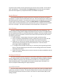
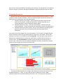
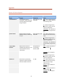
 The
Creating Defensible SLIMEstimate Solutions
HOW TO SPECIFY PROJECT ASSUMPTIONS AND CONSTRAINTS,
AND ANALYZE ALTERNATIVES
TableofContents
.............................................................................................................................................. 0 The ........................................................................................................................................ 0 Understanding Solutions Methods ............................................. Error! Bookmark not defined. Detailed Method ................................................................................................................... 3 Quick Estimate ...................................................................................................................... 3 Working Backwards??? ........................................................................................................ 3 Level of Effort Estimate .................................................................................................... 3 Solve for PI ........................................................................................................................ 4 Solve for Size ..................................................................................................................... 4 Leveraging SLIM Companion Products ..................................................................................... 4 Create Solution from SLIM‐DataManager ............................................................................ 4 Create Solution from SLIM‐Control ...................................................................................... 5 Solution Assumptions ............................................................................................................... 5 Phases ................................................................................................................................... 5 Expected Total Size ............................................................................................................... 6 Productivity Index (PI) .......................................................................................................... 6 Defect Tuning Factor ............................................................................................................ 6 Phase Tuning......................................................................................................................... 6 Accounting ............................................................................................................................ 7 Constraints .................................................................................. Error! Bookmark not defined. Comparing Alternatives ............................................................................................................ 9 Presenting Defensible Estimates .......................................................................................... 9 Appendix ................................................................................................................................. 10 Matrix of Solution Options ................................................................................................. 11 1 WhyReadthisDocument?
There are many factors that contribute to software development project success. SLIM‐
Estimate can simulate a majority of these factors, enabling you to anticipate potential outcomes, and equip your team to plan and act accordingly. As part of SLIM‐Estimate Best Practices series, this guide highlights SLIM’s Solution Methods and Solution Assumptions. It also explains how to perform comparative analysis, and why that is important. Key principles behind SLIM’s estimation process include:  A range of Solution Options are available to take advantage of available data. You can us the QSM industry database to supplement your historical data, in part or in whole. Estimates can be built directly from either SLIM‐DataManager or SLIM‐Control projects.  SLIM ‘Wizards’ allow you to view the project from different angles. The software production equation is rearranged to solve for different variables, size or PI in particular, to back‐calculate the product size and capability implied by your effort and schedule constraints.  Six data types within Solution Assumptions combine to uniquely model your project. Review all of them, and run multiple scenarios to consider a range of possible outcomes.  SLIM produces risk profiles for effort, cost, and schedule, so you can select the solution that meets your goals. Setting constraints with target probabilities calculates the amount of risk buffer you need to commit to an estimate solution.  Different from Solution Options, Solution Methods tell SLIM how to perform the simulation in order to optimize on your goals. Different methods will result in different solutions. ProducingYourFirstEstimate
Estimating with SLIM requires some planning and forethought. You must understand the project business goals, and the unique characteristics of the development environment. The product complexity, team productivity, and resource constraints are equally important determinates of the project outcome. The uncertainty about any of these values contributes to project risk, thus a main objective of your Requirements
Σ= Total Size
Resources &
Constraints
Software Elements
Initial Estimate
Tasks, Effort
Commitment
1 Process Productivity
Alternative
Scenarios
estimate is to obtain the best available data to support a thorough analysis of all the alternatives. Before you begin, take a moment to gather size, staffing, and productivity information for the project. These will become the primary inputs to the estimate. If this information is not available, don’t worry. SLIM‐Estimate will supply industry‐based default settings to guide you. The inputs you need are: •
Team size ‐ number of FTE (Full Time Equivalent) people you plan to use at the peak of the code and test phase. •
PI – productivity determined from one or more similar completed projects. If you don’t have this information, most templates contain both domain‐ and industry‐specific trends to help you pick a safe, reliable PI. Consult QSM’s Understanding SLIM‐Estimate Inputs reference for detailed information on determining PI. •
Effective Size – product measure gleaned from project artifacts. Again, if you don’t have these, most templates have at least one sizing method built right into the Size Calculator. And don’t forget to check out the Sizing Spreadsheets in the Samples and Templates folders of your application directory! The sample spreadsheets (.xls) contain a variety of sizing methods and gearing factors. Consult QSM’s Understanding SLIM‐
Estimate Inputs reference for detailed information on estimating size. •
Constraints – limitations on the budget of time, effort, team size, and cost that drive SLIM’s effort‐time trade‐off calculations. Prioritize them, so you can rank alternative solutions. To create a new estimate based on a template, select File | New from the menu and check Import Settings from Existing Template. Browse to the directory where your template is stored and select it. Since you’ve already customized your Project Environment settings, you should be able to focus on entering the assumptions, and select the best solution options. UnderstandingSolutionOptions
SLIM offers seven ways to build an estimate. The method you choose will be determined by the amount and detail of your input data, the type of problem you need to solve, and the time available to create the estimate. The complete menu of solution methods is presented on the New Project Options screen, presented when you are creating a workbook. Once you have opened an existing workbook file, the “Wizard” solutions methods may be accessed from the Estimate menu. The SLIM‐Estimate User Manual thoroughly explains each solution method. Review each of the methods in 2 conjunction with the data you have gathered to plan the best way to precede. An overview of each is provided here. Take advantage of the Solution Log and use more than one method (where the data supports it) to explore alternatives and validate assumptions. DetailedMethod
The Detailed Method allows complete control over the project environment and solution assumptions. It requires the most information from you. This is the method you normally select when working from a template. The project environment has been configured, so you can focus on entering the solution assumptions. Review the Global Options and Project Environment screens as they are presented, however you may skip them if you are familiar with the template with which you began. The solution assumptions are presented later in this document. QuickEstimate
The Quick Estimate option generates a baseline estimate that can be refined later. This solution produces a Rough Order of Magnitude (ROM) estimate using most of the QSM defaults. Use this method when either very little historical data is available, or the time available to build the estimate is severely shortened. A series of five screens will be presented so you can enter the following information. 1. Project Definition: Project Name, Phases to be included, and the Start Date. 2. Primary Trend Group: QSM database trends, by application type, that match the new project. This will determine the Size and PI data in the estimate calculations. 3. System Size: An intuitive size estimate selected from the Primary Trend Group, or a numerical value representing the most likely software size. Enter the relative percentage of New and Modified code. 4. PI: Average PI from the QSM Trend Group, or a numerical value representing the most likely PI. Postpone adjusting this value until the initial staffing profile can be reviewed with project participants. 5. Project Constraints: Highest priority resource constraint to balance probabilities and the effort‐time trade‐off. WorkingwithWizards
The normal estimation process calculates the total effort and duration required to build the system, using estimates of size and productivity. Rearranging the software production equation to solve for different parameters lets you determine the staff, size, or PI implied by specific effort and duration goals. These methods can be used to evaluate other’s estimates, or to ensure a complete understanding of the project dynamics. LevelofEffortEstimate
The Level of Effort Wizard is designed to allow you to specify the resources available and the productivity you expect to achieve. The wizard will determine the amount of functionality that can be built and the amount of time it will take. Enter either the Phase 3 effort (PM) or peak staffing available. 3 SolveforPI
The Solve for PI Wizard is designed to allow you to specify the size of the system and the resources available. This solution will produce a PI value mapping to the project’s duration and effort. Select either Peak Staff or person‐months to represent typical effort values. SolveforSize
The Solve for Size Wizard is designed to allow you to specify the resources available as well as the productivity level you expect to achieve. Enter the PI, time, and either the Phase 3 effort (PM) or peak staffing available. LeveragingSLIMCompanionProducts
It is always best to use your own history as the basis for estimating projects. Two solutions methods let you create an estimate based upon the characteristics and performance of specific projects for which you have detailed and/or summary level data. In addition to using SLIM‐
DataManager to begin a new estimate, you can use it to create a SLIM‐Estimate model of a completed project that has only total values for effort, duration, and size. For example, if you have total effort, size, and duration for a past project, but no phase or WBS level detail, combining this data with the template’s phase tuning settings models the actual performance at a more detailed level. This gives insight into how to adjust SLIM for the current estimate. CreateSolutionfromSLIM‐DataManager
Use this option when data for at least one completed project is available. The data many not already exist is a SLIM‐DataManager file, but can be entered prior to using this option. There are two approaches: 
Complete Data Set – If a SLIM‐DataManager database if available, identify the project to be used to create the SLIM‐Estimate template. Only one project can be used. Phase duration and shape, size, PI, MBI, milestones, application type, and all other project environment data will be imported if available. Missing, incomplete, or inconsistent information will be provided from QSM default settings. Key estimating parameters (Size, PI, MBI, phase time, effort, and overlap tuning factors) are imported and used to generate a new solution. 
Minimum Data Set – This solution should be used when only total duration, total effort, and total size can be determined, either from a past project, or for the one being used for tool configuration. Open SLIM‐DataManager, select File New, Add a Project. Enter the Project Name, Size, and minimum Phase 3 Data (Start Date, End Date, Effort, Peak Staff). Save the file and then proceed with SLIM‐Estimate configuration 4 CreateSolutionfromSLIM‐Control
This solution is similar to the previous one, but uses a SLIM‐Control file instead of a SLIM‐
DataManager file. SolutionAssumptions
The power and utility of SLIM‐Estimate is the ease with which different combinations of assumptions can reveal important trade‐offs among Size, PI, Effort and Duration. Most of the other configuration data (Project Environment and Global Options) is static across projects of the same type, whereas the assumptions entered here are unique to each project. Be sure and take advantage of the Solution Log to document any changes as you refine the estimate. The Description field provides ample space to explain data sources or reasoning behind the assumption. Phases
If you are starting from a pre‐configured template, the phase descriptions and curve shapes have already been set. Verify that the phase activities to be performed on the current project match those in the template. It is not uncommon for many projects to conduct only Phases 2 and 3. Change the Rayleigh curve shape to adjust whether the peak staff occurs early or late in the phase. If you are using a pre‐configured template, do not alter these settings without checking with experienced team members. 5 ExpectedTotalSize
Expected Total Size results from the combined effect of each data element on this screen: Function Unit (Total ‘FU’), Gearing Factor, percent New, Modified, and Reused functionality, and the Uncertainty Range. If the Function Unit is the same as the Basic Unit of Work (see Global Options and Project Environment data tabs), the Gearing Factor is 1. Total ‘FU’ can be entered directly, or computed using the Sizing Calculator. Keep in mind that the range of uncertainty will translate to a corresponding level of variability around the resulting effort and duration predictions. Set the range to reflect your confidence in the size estimate. See QSM’s reference Understanding SLIM‐Estimate Inputs for detailed instructions for selecting and using one or more of the techniques in the Sizing Calculator. ProductivityIndex(PI)
You can enter the expected PI directly into the field, or allow SLIM to roll up the value from the PI Calculator. The PI History option is only available if you have loaded historical projects into the template. It is a good idea to use this option, even if you only have one project, because it documents the source of the PI data if you are not using the QSM database. As with Expected Total Size, the range of uncertainty will translate to a corresponding level of variability around the resulting effort and duration predictions See QSM’s reference Understanding SLIM‐Estimate Inputs for detailed instructions for selecting and adjusting productivity using in the PI Calculator. DefectTuningFactor
The Defect Tuning Factor is a scaling parameter that tunes SLIM‐Estimate’s reliability model up or down to match your historical defect discovery data. For each historical project you have loaded into the current workbook, a Defect Tuning Factor will be calculated (if you have provided defect data). If you have not loaded historical data, the defect curves will be determined from the Primary Trend Group. The display will read as 100%, indicating the QSM default prediction will apply. PhaseTuning
The Phase Tuning options give you a great deal of flexibility in modeling SLIM’s four development phases to your environment. You can specify three variables: phase Start, Duration, and Effort. Additionally you can set the overlap with the next phase. SLIM performs the estimate calculations for Phase 3. Time and effort for Phases 1, 2, and 4 are then generated as percentages of phase 3. Each phase has its own tab, allowing you to configure each active phase independently. This is particularly 6 helpful when you have different teams performing different activities. Exercise caution in modifying the phase overlap, so you do not overcommit available resources. As with the Defect Tuning Factor, you can take advantage of historical project data and tune the phases to match like development plans. The PI and MBI (Manpower Buildup Index) correlate to this data to give a complete picture of how the project was run. If you began your estimate with a custom template, the phase tuning may have already been set, in which case you want to confer with team members before making modifications. Accounting
Setting the person‐hours per person‐month value ensures proper determination of peak staff and total effort distribution. Enter the average labor rate and corresponding effort unit for accurate cost calculations. Labor rates may be entered for each Skills Category, enabling you to can view project costs by role for each phase and over the entire life cycle. Since SLIM‐Estimate works with the overall average labor rate to generate the overall cost estimate for the current solution, click on the Update Labor Rate button to sync up the labor rates on your final solution. SolutionMethod
The SLIM‐Estimate User Manual describes when and how to use each of the Solution Methods on the Solution Assumptions screen. The default is Unconstrained. Once the first solution is displayed, you will see that the radio button moved to the Design to input method. This is because once SLIM determines the MBI (Manpower Buildup Index), it assumes you want to hold that value constant unless otherwise indicated. You can use this method to optimize your estimate to meet a critical project goal or objective. For example, you can design to Peak Staff or Life Cycle Cost. That way, instead of optimizing on 7 a solution that balances effort, time, and staff, SLIM determines the requirements to meet your most important goals. Constraints
Select the Constrained Solution option to limit the range of possible solutions to important project limitations. Often, the allotted time budget for the project is less than adequate. Limiting the project duration to, say 15 months, may be a legitimate business need, or it may be set arbitrarily. There are limits to the number of human resources available as well, expressed as either total effort or peak staff. Entering a constraint in SLIM‐Estimate bounds the available solutions in order to meet the target probability. You can assign a target probability to each constraint. Typically, this is a value between 50% and 99% with a default setting of 80%. The target probability indicates how certain you would like to be of achieving each goal, and determines the amount of risk buffer SLIM builds into your estimate. Note: there are two ways to use constraints. Adding constraints via the Estimate | Constraints menu item allows you to display the current solution against your constraints on risk panels, but does not generate a new, constrained solution. You can also set constraints via the Solution Assumptions dialog, Edit Constraints button. Setting constraints in this way will cause a new solution to be generated when you exit the Edit Constraints dialog and click OK on the Solution Assumptions dialog 8 (note that the Constrained Solution method must be selected). This will generate a risk‐buffered solution using your constraints and target probabilities to add in the desired amount of buffer. ComparingAlternatives
Now that you have entered your assumptions and generated at least one solution, it is time to explore multiple possible outcomes. There are a few meaningful comparisons that help you determine which solution best meets the projects goals:  Compare solutions to each other – tells you which assumptions have the most impact on the outcome. Should we decrease the schedule, decrease size, or increase the effort in order to achieve the project goals?  Compare solutions to history – tells you if the estimate is consistent with your known capabilities. Are you attempting to do something you have not done before?  Compare solutions to industry trends – tells you if the estimate is something that is generally reasonable. Are we attempting to do something impossible or impractical? Log a solution each time change one or more assumptions. To view the list of logged solutions, click on the down arrow to the right of the Solutions combo box in the toolbar. You can edit solutions or see them in more detail by selecting Log | Edit… from the menu. Each solution is displayed as a red dot (default) on comparison scatter plots. Loaded historical projects are shown in black. The Current Solution, selected from the pull‐down list on the menu bar, is shown in blue. Due to the non‐linear relationship between size, effort, and duration, compare projects that are roughly the same size for best results. The solid trend line represents the average, and dotted lines represent plus and minus one Standard Deviation (+/‐ 1 STD). You may alter the charts to display up to 3 STD. QSM experience shows that reasonable estimates fall within 1 STD. To interpret the comparison 9 charts, notice whether the Current Solution is above or below the average. In the Life Duration chart above, you can see that for a project of similar size, this solution predicts a life cycle duration 1 STD less than what would be typical. The Life Effort chart indicates an even larger discrepancy – over 1 STD less effort than typical. This analysis prompts you to determine why, and decide if the cause is acceptable. PresentingDefensibleEstimates
There is wide range of views contained in the QSM default template. The sections (folders) in the navigation panel are arranged in a logical sequence, grouping like views together. Once you have selected the best estimate, select a handful of views that support your decision. If you ran more solutions than you want to present, you can opt to hide logged solutions from view with Log | Edit feature. You should decide if you want to present the charts and reports using SLIM‐Estimate, or if it would be better to export them to another program. To use another program, select File | Export Workbook and choose the desired output format. Microsoft (MS) PowerPoint is the most common presentation package used. If you select this option, you will be asked to supply a file name, the next screen displayed lets you specify exactly which views to export. Alternatively you can select Edit | Copy View to Clipboard, and then past the view into your application of choice. A defensible estimate is one that has explored a variety of potential outcomes, and readily answers common “what if” questions from management, like:  What if the Size is 20% larger?  What if we do not have access to all of the people we predicted?  How much can we compress the schedule by adding more effort? Reserve one or two alternative solutions you would recommend in addition to the best one, and be prepared to discuss the relative merits of each. One final note is to remember that your estimate should be refined once the project starts and more detailed information is available. Perform estimates after the completion of requirements and design activities, to improve size estimates. If the project plan must be altered, it is best to do it as early as possible. 10 Appendix
MatrixofSolutionOptions
Name Purpose Solves For Input Detailed Method Enter detailed solution assumptions, taking advantage of historical data and multiple sizing techniques. Effort, Duration, Peak Staff, MBI Size ‐ Enter a single expected value, or use Sizing Calculator. Enter Gearing Factor PI ‐ Accept average PI from the trend, or enter your own. Adjust as appropriate. Uncertainty ‐ Use slider bar to set uncertainty range for Size & PI. Quick Estimate Rough estimate using QSM database Primary Trend Group as input. PI ‐ Accept average PI from the trend, or enter your own. Adjust as appropriate. Uncertainty ‐ Use slider bar to set uncertainty range for Size only. Level of Effort Estimate Specify human resources Size (Amount of available and productivity. Size Functionality), determined from Primary Duration, MBI Trend Group. Effort ‐ Phase 3 total effort in Person‐Months; or Peak Staff ‐ No. of People in Phase 3 PI ‐ Accept average PI from the trend, or enter your own. Adjust as appropriate. Solve for PI Determine the productivity required to achieve specified Size with available resources. Duration ‐ Max available for entire project. Effort ‐ Phase 3 total effort in Person‐Months; or Peak Staff ‐ No. of People in Phase 3 11 Effort, Duration, Peak
Staff, MBI PI, MBI
Size ‐ Select relative size via slider bar; Very Small to Very Large Size ‐ Select relative size via slider bar; Very Small to Very Large, or Enter a single expected value. Solve for Size Specify human resources Size, MBI
available and productivity. Size determined from Primary Trend Group PI ‐ Enter the PI expected to be achieved. Duration ‐ Max available for entire project. Effort ‐ Life cycle total effort in Person‐Months; or Peak Staff ‐ No. of People in Phase 3 12