1
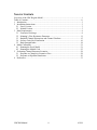
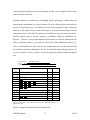
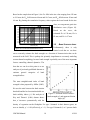
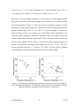
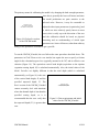
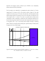
THE UNIVERSITY OF BRITISH
COLUMBIA REGIME MODEL (UBCRM)
USER’S MANUAL
DEPARTMENTS OF CIVIL ENGINEERING & GEOGRAPHY
THE UNIVERSITY OF BRITISH COLUMBIA
October 2007
© Brett Eaton, 2007
OVERVIEW OF THE UBC REGIME MODEL
The UBC Regime model has been developed over a number of years in collaboration
between researchers in the Department of Civil Engineering and the Department of
Geography at the University of BC. The model is based on the understanding that a
simple model with modest data requirements is more likely to be useful than a data
intensive, numerically demanding one, especially for environmental practitioners. While
simple, the model does consider the relevant controlling factors, the most important of
which is the nature and erodibility of the channel banks. The goal of our research on this
topic is to determine which simplifying assumptions about river channel behaviour are
reasonable to make, and to identify the underlying physical processes. The version of the
model presented here can be calibrated for a field site, and then used to evaluate how the
field site could potentially respond to changes in the formative discharge, bank strength
or any of the other governing conditions related to channel morphology in the model.
Rational regime theories relating stream channel conditions to the external driving forces
have a long history (Chang, 1979; Davies and Sutherland, 1983; Ferguson, 1986; Kirkby,
1977; White et al., 1982; Yang, 1976). There are two main impediments to the general
acceptance of rational regime models: the first is the development of a scientifically
reasonable understanding of the extremal hypotheses used in the models; and the second
is the incorporation of a bank stability analysis in the model. Researchers at UBC
(including M. Church, B. Eaton, R. Millar, M. Quick) have made significant progress on
these two issues. We have been able to re-formulate the extremal hypotheses in such a
way as to make the underlying principle more easily understood (Eaton et al., 2004;
Millar, 2005). We have tested this principle against observed channel adjustments in the
laboratory and in the field, where we have observed behaviour that is consistent with our
generalized extremal hypothesis (Eaton and Church, 2004; Eaton and Church, 2007;
Eaton and Millar, 2004). We have also incorporated various bank strength formulations
into the regime model which results in a general agreement between model predictions
and observed channel dimensions, overcoming the long-standing criticism that regime
models consistently under-predict channel width (Eaton, 2006; Millar, 2005; Millar and
Quick, 1993; Millar and Quick, 1998). The regime model is gaining recognition, and was
awarded the Wiley Award by the British Geomorphological Research Group for best
paper in ESPL for 2004/05. It is now being tested by various researchers and
environmental consultants in BC who are looking for practical tools for making better
decisions about stream channel management. We believe that there are numerous
potential applications for this model, including the replacement of arbitrary and
theoretically meaningless hydraulic geometry equations in numerical models of
downstream sediment transfer and longitudinal profile evolution, and landscape
evolution.
UBCRM Manual
i
6/5/08
TABLE OF CONTENTS
Overview of the UBC Regime Model ................................................................................. i
Table of Contents................................................................................................................ ii
1 Introduction................................................................................................................... 3
2 Installation Instructions................................................................................................. 3
2.1 Excel Version......................................................................................................... 3
2.2 Matlab Version....................................................................................................... 5
3 Data Requirements........................................................................................................ 8
3.1 Formative Discharge.............................................................................................. 8
3.2 Manning’s Flow Resistance Parameter................................................................ 11
3.3 Bankfull Channel Dimensions and Channel Gradient ......................................... 15
3.4 Surface Grain Size Distribution ........................................................................... 16
3.5 Bank Strength Index ............................................................................................ 18
4 Model Calibration ....................................................................................................... 21
4.1 Running the Excel Model .................................................................................... 21
4.2 Running the Matlab Code .................................................................................... 25
5 Evaluating Channel Response Scenarios .................................................................... 28
5.1 Response to Changes in Formative Flow............................................................. 28
5.2 Response to Riparian Disturbance ....................................................................... 30
6 References................................................................................................................... 33
UBCRM Manual
ii
6/5/08
1
INTRODUCTION
The regime model can be run from two different platforms. The most widely accessible
platform is Excel, where the program relies on the Solver Add-in component to seek
numerical solutions. The most flexible (and useful) platform is the numerical analysis
program, MATLAB 1 (http://www.mathworks.com/). This user’s manual presents the
instructions for installing and running both versions of the program, and provides some
examples of how the model can be used, practically.
2
INSTALLATION INSTRUCTIONS
2.1
EXCEL VERSION
To install the UBCRM program, simply copy the Excel file UBCRM.xls to your hard
drive, and then open the file with Excel. The file contains four worksheets, entitled notes,
CRB_Eq, UBCRM and UBCRM_H, respectively. The notes page is intended to be used to
temporarily (if not permanently) store the results of various analyses run by the model,
and is no different than any other blank worksheet in Excel. Additional sheets for storing
simulation results can be created by clicking on the Insert menu, then on Worksheet from
the list of options in that menu. The CRB_Eq sheet contains a set of equations that
generate first approximations of the channel dimensions based on a reduced set of input
parameters. The other two sheets contain a series of cells into which the user must enter a
complete set of input parameters characterizing the river system under consideration, and
other cells whose values are determined by the values the user enters. The UBCRM
model contains the regime model based on Millar and Quick’s (1993) bank stability
analysis. The UBCRM_H model contains a regime model based on Eaton’s (2006) bank
stability analysis. Both models function in essentially the same way.
To run the complete UBCRM and UBCRM_H models (see Section 4 for details), the user
enters the required data values and then selects the Solver tool from the Tools menu. The
1
The freely available program, Octave (http://www.gnu.org/software/octave/octave.html), may also be
capable of running the MATLAB scripts. However, this manual does not explicitly cover installation and
running the program in Octave.
UBCRM Manual
3
6/5/08
user must be on the worksheet for the model that they wish to run in order to access the
appropriately configured Solver: Solver is accessible from any worksheet, but the settings
(which have already been specified in the Excel program) are customized for each
worksheet. Figure 1 shows the Solver window and Solver parameters for the UBCRM
model; Figure 2 shows the window and parameters for the UBCRM_H model.
QuickTime™ and a
TIFF (LZW) decompressor
are needed to see this picture.
Figure 1: Solver parameters for UBCRM
QuickTime™ and a
TIFF (LZW) decompressor
are needed to see this picture.
Figure 2: Solver parameters for UBCRM_H
If you do not see the Solver tool in the Tools menu, then it has not been installed on your
machine. It is an add-in program, as described in Figure 3. This is a two-step process,
UBCRM Manual
4
6/5/08
involving first installing the add-in on your computer, then loading the add-in into Excel.
The procedures for doing this vary with the version of Excel being used, so please consult
the Excel Help menu for details.
QuickTime™ and a
TIFF (LZW) decompressor
are needed to see this picture.
Figure 3: Excel help for add-in programs
It is recommended that you keep a backup copy of the original UBCRM.xls file on your
hard drive, and create working copies in which to conduct analyses: saving the program
under a different name has no effect on how the program works. Should the formulae in
the working spreadsheet or the settings in the Solver program become irrevocably
changed, then reverting to the backup file should fix the problem.
2.2
MATLAB VERSION
First, you need to have a working copy of MATLAB. The programs were written with
MATLAB version 7.4.0 (R2007a). There are two versions of the MATLAB code, located
in two separate folders. The folder UBCRM_files contains the programs necessary to run
a regime model using Millar and Quick’s (1993) bank stability analysis. The folder
UBCRM_H_files contains the files for a model using the stability analysis presented by
UBCRM Manual
5
6/5/08
Eaton (2006). Each folder contains one main program file (UBCRM.m and UBCRM_H.m,
respectively) that runs the regime model and three sub-programs (also .m files) that are
called by the main program. There is also a file that keeps track of the last input values
used in the model (UBCRMdef.mat and UBCRMHdef.mat).
To install these programs, copy the folders onto your hard drive. Then, in MATLAB, add
the folders to the path. In the File menu, select Set Path. Then, click on the Add Folder
button in the Set Path window (Figure 4) and navigate to the folder for the program you
are installing (UBCRM or UBCRM_H), and click Open. This will add the folder to the list
of directories in which MATLAB will look for programs, and you will return to the Set
Path window. Then click on Close in the Set Path window. MATLAB will then ask you
if you want to save the changes to the path: if you want to permanently add the folder to
the path (and the program to the set of programs that MATLAB can access every time it
is opened), click Yes, if you prefer to set the path every time you want to use the program,
click No.
QuickTime™ and a
TIFF (LZW) decompressor
are needed to see this picture.
Figure 4: Set Path window in MATLAB
To run the main program, type UBCRM or UBCRM_H on the command line, then press
enter. Assuming that you are using the UBCRM version, if you get the message undefined
UBCRM Manual
6
6/5/08
function or variable ‘UBCRM’, then the path has not been set properly. Other error
messages are likely to indicate that the code has been changed in the .m files that execute
the program, or that one or more of the sub-programs are missing. Note that the file
names are case-sensitive, and file transfer between operating systems can result in
changes to the file name cases. The file names as they are meant to appear are shown in
Figure 5 and Figure 6: if the file names have been changed to all upper case or all lower
case letters, you will have to change them back to their original case-sensitive names, as
shown.
QuickTime™ and a
TIFF (LZW) decompressor
are needed to see this picture.
Figure 5: Case-sensitive file names for UBCRM version of the regime model
(MATLAB code)
QuickTime™ and a
TIFF (LZW) decompressor
are needed to see this picture.
Figure 6: Case-sensitive file names for UBCRM_H version of the regime model
(MATLAB code)
UBCRM Manual
7
6/5/08
3
DATA REQUIREMENTS
In order to set up and run the model, it is necessary to have information on the stream
channel under consideration: this usually requires measurements taken in the field. The
model requires an estimate of the formative discharge for the channel, the characteristic
Manning’s flow resistance parameter at the formative discharge, and the reach-average
channel slope. It also requires knowledge of the range of grain sizes found on the bed
surface of the channel, and of the relative erodiblility of the channel banks. The following
sub-sections define the input variables that the model requires and describes how suitable
estimates can be determined.
3.1
FORMATIVE DISCHARGE
The regime model is predicated upon the idea that channel morphology is related to the
flows carried by the stream, averaged over some suitably long timescale (see Eaton et al.,
2004). Gravel bed streams only ever mobilize their bed material during periods of
relatively high flow. The bankfull flow (which is the discharge that just fills the channel
up to the level of the floodplain surface) is the best representative of the formative
discharge, since flows less than bankfull are not capable of doing much geomorphic work
and since flows greater than bankfull spill out onto the floodplain, contributing little to
the flow acting directly upon the stream channel.
For streams that are gauged, estimating the formative discharge is relatively
straightforward. In Canada, the Water Survey of Canada (WSC) collects and archives
data on streamflow for selected streams. The available data can be downloaded from the
WSC website (http://www.wsc.ec.gc.ca/index_e.cfm?cname=main_e.cfm). An example
of a typical data report from WSC is shown in Figure 7. The WSC provides estimates of
the maximum instantaneous peak flow in each year of record, as well as the highest
average daily discharge for each year (referred to as the maximum daily discharge). Since
channel morphology changes over relatively long time periods, it is probably most
appropriate to use an average of the maximum daily discharge values to estimate the
formative discharge. Given that the climate variability produces shifts in stream flow
UBCRM Manual
8
6/5/08
regimes (e.g. Moore, 1996), it is probably best to represent the formative discharge using
a 5-year to 10-year average immediately prior to the period of interest.
QuickTime™ and a
TIFF (Uncompressed) decompressor
are needed to see this picture.
Figure 7: Sample WSC data for Fishtrap Creek
UBCRM Manual
9
6/5/08
In general, the average mean annual peak flow (estimated from stream flow records) is
similar to the bankfull discharge (which is determined by the average channel
morphology). However, if one is considering streams in arid regions, the formative
discharge may be much less frequent, and the evidence of large, infrequent floods may
persist over decades or even centuries (Baker, 1977). The range in peak flow magnitudes
also tends to be higher in more arid regions, which can also affect the frequency of the
formative discharge. For example, analysis of the streams in Colorado described by
Andrews (1984) by Eaton and Church (2007) seem to be associated with formative
discharges having return periods of about 10 years (i.e. the flows likely to be equaled or
exceeded only once in any 10-year period of record).
When there are no stream discharge measurements on the stream of interest, it is
sometimes possible to estimate the formative flows using regional hydrology analyses.
For example, Eaton et al. (2002) present a regional analysis of the peak flows for British
Columbia for the mean annual peak flow, as well as some less frequent peak flows. The
present a general equation that relates discharge (Q) to drainage area of the form:
Eq. 1
Q = kA 0.75
where k is the discharge for a drainage area of 1 km2, and A is the drainage area in km2.
Eaton et al (2002) present a map 2 of k-factors for British Columbia, which is reproduced
here in color (Figure 8). Eaton and Moore (2007) also discuss the variation of peak flows
(as well as the peak flow generating mechanisms) in BC.
Eq. 1 really amounts to a scaling equation that accounts for the fact that peak flows are
not linearly related to drainage area. It can be used (in BC, at least) to take data for one
basin and use it to characterize another, ungauged basin. The first step is to obtain a k
value for your drainage basin. In BC, k values can be read from the map in Figure 8,
which presents Eaton et al.’s analysis. One can also estimate k values for an ungauged
2
A geo-registered TIF file of this map can be downloaded from Brett Eaton’s web page:
(http://www.geog.ubc.ca/~beaton/downloads.html)
UBCRM Manual
10
6/5/08
study site using a nearby gauged catchment, since both Q and A are known (k = Q/A0.75).
The estimated k value can then be used to estimate the formative discharge for the study
site, though differences in the catchment physiography and climatology will produce
large uncertainties in the estimate. It is therefore recommended that any region peak flow
estimate be checked against the observed channel dimensions in the field, as described
below.
QuickTime™ and a
TIFF (Uncompressed) decompressor
are needed to see this picture.
Figure 8: Map of k-factors, presented in Eaton and Moore (Eaton and Moore, 2007)
3.2
MANNING’S FLOW RESISTANCE PARAMETER
This parameter has a significant effect on the model predictions, so getting a reasonable
value is critical. There are a number of references that can be used to estimate flow
resistance. For example, Cowan’s (1956) method is a useful approach, since it attempts to
UBCRM Manual
11
6/5/08
attribute flow resistance to various components of the river form. His equation takes the
form:
n = (n o + n1 + n 2 + n 3 + n 4 )m 5
Eq. 2
The parameters and typical values are given in Table 1. This is a reasonable technique to
apply to large rivers (c.f. Church, 1992), provided the channel gradient is not too high.
However, since this scheme relies heavily on the qualitative judgment of the individual
assessing the stream channel, the predicted value of n is strongly dependent on the
individual making the assessment in the field. It is recommended that the field crew take
numerous photographs to document the channel conditions in order to allow the various
judgments to be re-evaluated, if necessary.
Table 1: Cowan’s (1956) method for estimating Manning’s n
Parameter
Sediment Type, no
Values
Earth
Rock cut
Fine gravel
Coarse gravel
Degree of cross section irregularity, n1
Smooth
Minor
Moderate
Severe
Downstream variations in cross section shape, n2
(e.g. thalweg shifts from side to side)
Gradual
Alternating occasionally
Alternating frequently
Relative effect of obstructions, n3
(e.g. logs, boulders)
Negligible
Minor
Appreciable
Severe
Vegetation, n4
Low
Medium
High
Very high
Degree of meandering, m5
Minor (sinuosity 1.0 to 1.2)
Appreciable (sinuosity 1.2 to 1.5)
Severe (sinuosity greater than 1.5)
UBCRM Manual
12
0.020
0.025
0.024
0.028
0.000
0.005
0.010
0.020
0.000
0.005
0.010 to 0.015
0.000
0.010 to 0.015
0.020 to 0.050
0.040 to 0.060
0.005 to 0.010
0.010 to 0.025
0.025 to 0.050
0.050 to 0.100
1.00
1.15
1.30
6/5/08
The Cowan method (and most other commonly used methods) perform poorly in steep
mountain streams (Marcus et al., 1992). According to Chow (1959), mountain streams
with gravel-cobble boundaries have Manning’s n values that average 0.040 (ranging from
0.030 to 0.050). Mountain streams with cobble-boulder boundaries have higher
Manning’s n values (mean of 0.050, ranging from 0.040 to 0.070).
Jarrett (1984) presents an equation for mountain streams (0.02 < S < 0.04) that relates n
to channel slope (S) and the hydraulic radius (approximated here using the mean
hydraulic depth, d):
Eq. 3
n = 0.32S 0.38 d −0.16
However tests of this equation indicate that it tends to over-predict Manning’s n by, on
average, about 30% (Marcus et al., 1992).
Bathurst (2002) presents a formula for estimating the minimum flow resistance in streams
with gradients less than 0.08 m/m. His formula was originally used to estimate the Darcy
Wiesbach friction factor. Rearranging to give estimates of n yield the equation:
Eq. 4
n=
0.547
R1/ 6 ⎛ D84 ⎞
⎜
⎟
3.84 g ⎝ d ⎠
where D84 is grain size for which 84% of the surface grains are finer (see section on grain
size distribution for a description of how to collect and analyze the relevant data), and d
is the mean hydraulic depth. The parameter g is the acceleration of gravity (9.8 m/s2). R is
the hydraulic radius of the channel 3 , given by the ratio of the cross sectional area for flow
(A) and the wetted perimeter of the channel (P): R = A/P. If we interpret Jarrett’s equation
as an upper bound and Bathurst’s equation as a lower bound, we should expect the
3
In wide, shallow channels, the hydraulic radius, R, is nearly identical to the mean hydraulic depth, d.
UBCRM Manual
13
6/5/08
average of the two to produce a reasonable estimate of the likely Manning’s n value. We
can also use the upper and lower bounds to test the sensitivity of the model to the choice
of n values that are selected.
The best (and most difficult) option is always to use field measurements to backcalculate n values for a study site. This requires that the stream flow at or near the
bankfull discharge be directly measured. If the cross sectional area of flow (A, in m2), the
mean water surface width (W, in m) and mean water surface gradient (S) are also
measured, n can be estimated from the following equations:
Q = Av = Wdv
Eq. 5
where Q is the discharge (m3/s), and v is the mean velocity. Manning’s equation is:
v=
Eq. 6
R 2 / 3 S1/ 2
n
Combining Eq. 5 and Eq. 6 and then isolating n, we get:
Eq. 7
Q=
Eq. 8
n=
(Wd)R 2 / 3 S1/ 2
n
(Wd)R 2 / 3S1/ 2
Q
≈
Wd 5 / 3 S1/ 2
n
≈
Wd 5 / 3 S1/ 2
Q
The values of W, d, R and S are those associated with the measured discharge, not the
bankfull channel dimensions. However, the bankfull channel dimensions (as surveyed at
low flow) can be used to estimate both the discharge and the flow resistance parameter n.
UBCRM Manual
14
6/5/08
3.3
BANKFULL CHANNEL DIMENSIONS AND CHANNEL GRADIENT
While it is usually quite difficult to gauge streamflow in a stream at near-formative flows,
it is much simpler to estimate and survey the bankfull channel dimensions. In the field,
the bankfull channel dimensions must be carefully identified, and several cross sections
should be surveyed in order to determine the average bankfull width and depth. The field
crew surveying the channel should take care to differentiate between low terraces
generated by either systematic or local channel degradation, since mistaking a low terrace
for a floodplain surface will dramatically inflate the estimated bankfull discharge.
Ideally, the field crew will be able to survey at least 10 channel cross sections with the
reach of interest, demarcating the top of bank, bottom of bank, edge of vegetation, any
indictors of the bankfull elevation (e.g. LWD accumulations, vegetated bar tops, clearly
active floodplain surfaces, etc.), the water’s edge at the time of survey, and the thalweg
location. They should also collect enough data to faithfully reproduce the general cross
section shape, but there is little to be gained by a hyper-detailed survey of the details of
the cross sectional topography. Cross sections should be regularly spaced, about one to
two channel widths apart from each other. An automatic level and stadia rod is adequate
for this sort of survey, but care must be taken when reading and recording the upper,
middle and lower stadia values, since reading and transcription errors are common. The
preferred methodology for surveying channel cross sections is to use a Total Station to
survey the cross sections. While these instruments are more expensive and more
complicated to use, they are far more accurate and there are few opportunities for
mistakes to be make.
The average channel slope should also be surveyed as accurately as possible. The best
method for estimating the channel slope accurately is to construct a fairly detailed
longitudinal profile along the channel thalweg, recording the elevation of the thalweg as
well as the water depth and plotting those data against distance along the thalweg. Any
bedrock, boulder of LWD steps should be carefully surveyed, and the locations of the
surveyed cross sections should be noted on the longitudinal profile. The survey should
extend of multiple sequences of pools and riffles in order to determine a suitable reach-
UBCRM Manual
15
6/5/08
average slope. Once the survey data has been reduced and the longitudinal profile has
been plotted, a linear regression should be fit to both the bed elevation and the water
surface elevation data. While there will be trends in the data produced by sequences of
riffles and pools, there should not be any systematic changes in slope throughout the
study reach: such changes will show up at systematic deviations in the data from the
linear fit over distances greater than the riffle-pool spacing (which is about 3 to 7 channel
widths). If there are systematic changes in slope evident on the longitudinal profile,
consider subdividing the reach and fitting the linear regressions (and the regime model!)
to the upper and lower parts of the reach. If significant trends still persist, consider further
subdividing the reach.
In cases where there are no discharge measurements for the stream (i.e. no WSC gauge),
then stream discharge and Manning’s both need to be estimated from the bankfull
dimensions and the channel slope. Once bankfull estimates of W, d and S are known from
the channel survey, a value of n should be selected in order to estimate Q using Eq. 7.
Wherever possible, the resulting estimate of Q should be compared with estimates from
regional hydrology analyses (described above) in order to verify that (i) bankfull stage
was reasonably identified in the field and (ii) that the value of n selected was appropriate.
If necessary and justifiable, the value of n can be adjusted based on the results of this test.
The regime model simply uses n in conjunction with S and Q to estimate the channel
depth and from that the shear stress acting on the bed, so provided that the values of n, S
and Q associated with the surveyed bankfull channel are all entered into the regime
model, it should perform reasonably well.
3.4
SURFACE GRAIN SIZE DISTRIBUTION
Accurate information on the surface texture is also required to run the model. The median
grain size is used to estimate the sediment transport rate, and grain size characteristic of
the coarse tail of the distribution is used to assess channel stability and the flow resistance
parameter. The best means of determining the surface grain size distribution is by
conducting a surface Wolman sample. Samples should ideally be conducted on the
coarsest part of the bar heads in the study reach: the intent is to characterize the bed
UBCRM Manual
16
6/5/08
texture along the thalweg of the stream channel. Ideally, several samples will be taken
within the reach of interest.
Wolman samples are conducted by establishing regular grid using a flexible tape and
measuring the intermediate (or b-axis) diameter of every sediment grain at the nodes of
the grid. The grid spacing (i.e. the distance between nodes) should be at least 4 times the
diameter of the largest stone to ensure that there is no spatial autocorrelation between
subsequent stones on the grid. The grains are classified into one of several size classes,
and the frequency data is used to construct a cumulative frequency distribution (see
Figure 9). Typically, at least 100 grains must be measured to accurately characterize the
surface. Estimates of the D95 (the grain for which 95% of the distribution is finer), D84
(84% of the distribution is finer) and D50 (the median grain size) can be extracted from
the cumulative frequency distribution. The D95 is used for the bank stability analysis, D84
is used to estimate n in Eq. 4, and D50 is used to estimate the typical sediment transport
rate.
STUDY AREA:
FISHTRAP CREEK
DATE: SEPT. 29, 2007
SAMPLE LOCATION:
HEAD OF BAR 2, MID-REACH
NUMBER OF STONES
SIZE
CLASS
(mm)
256 – 181
P
(0)
128 – 181
1
90.5 – 128
1111
64 – 90.5
1111
45 – 64
1111
1111
1111
1111
32 – 45
1111
1111
1111
1111
22.7 – 32
1111
1111
16 – 22.7
1111
1111
11 – 16
1111
111
C.F.
1.00
(1)
0.01
0.99
1
(6)
0.06
0.93
11
(7)
0.07
0.87
1
(21)
0.20
0.67
1
(21)
0.20
0.47
1111
(15)
0.14
0.33
1111
(14)
0.13
0.20
(8)
0.07
0.13
8 – 11
11
(2)
0.02
0.11
5.6 – 8
11
(2)
0.02
0.09
(10)
0.09
0.00
< 5.6
1111
1111
Total
107
P is the number in each class divided by the total; CF is the total proportion of the distribution finer
than the given class (the Cumulative Frequency distribution) For a field sampling template, see
UBCRM_Forms.pdf.
Figure 9: Sample Wolman data from Fishtrap Creek
UBCRM Manual
17
6/5/08
Based on the sample data in Figure 9, the D95 falls in the size class ranging from 128 mm
to 181 mm, the D84 falls between 64 mm and 90.5 mm, and D50 falls between 45 mm and
64 mm. By plotting the cumulative frequency values against the lower bound for the size
class, we can generate grain size
1.00
distribution curve (Figure 10).
0.90
0.80
Based
0.70
0.60
on
the
curve,
the
estimated D95 is 130 mm, D84 is
0.50
0.40
85 mm, and D50 is 47 mm.
0.30
0.20
0.10
0.00
10
100
1000
Grain size (mm)
Figure 10: Grain size distribution curve
3.5
BANK STRENGTH INDEX
Unfortunately, there is only
limited work that we can draw
on to accurately estimate the bank strength as a function of characteristics that can be
measured in the field. This is perhaps the primarily impediment to accurately modeling
stream channel morphology because bank strength is probably one of the most important
factors controlling channel dynamics. The
best that we can do at this point is to use
analyses of previously published datasets to
estimate
general
categories
of
bank
strength indices.
The most straightforward index of bank
strength is that proposed by Millar (2005).
He uses the ratio between the bank erosion
threshold and the bed erosion threshold as a
bank stability index (μ′). His analysis of
Hey and Thorne’s (1986) dataset shows
Figure 11: Relation between relative
bank strength (μ′) and apparent friction
angle (φ′)
that μ′ increases systematically with the
density of vegetation on the floodplain. For type I channels in their dataset (grass, no
trees or shrubs), μ′ = 0.98 (effectively μ′ = 1). For type II channels (1 to 5 percent shrub
UBCRM Manual
18
6/5/08
or tree cover), μ′ = 1.17; for type III channels (5 to 50 percent shrub or tree cover) μ′ =
1.41; and for type IV channels (>50 percent tree or shrub cover) μ′ = 1.92.
This index is based on Millar and Quick’s (1993) original use of an apparent friction
angle (φ′) to characterize relative bank strength. The two indices are very closely related,
as shown graphically in Figure 11. There have been several analyses relating μ′ to Hey
and Thorne’s stream channel classes. For example Eaton (2006) calculated representative
apparent friction angles of 40o, 45o, 49o and 55o for types I through IV, respectively.
However, both μ′ (and φ′) vary with the size of the channel under consideration, even
when the riparian vegetation characteristic remain the same: for example see the data
analysis conducted by Eaton and Church (2007). Eaton and Millar (2004) conducted an
analysis which suggests that the effect of vegetation on bank strength disappears for
channels with formative discharges greater than about 400 m3/s: for Q > 400 m3/s,
streams will characterized by μ′ = 1.0 and φ′ = 40o, unless, of course, cohesive sediment
in the floodplain or other factors significantly affect relative bank strength.
Figure 12: Variation in φ′ with formative discharge for alluvial channels in the Salmon
River area (data from Emmett, 1975) and from streams in Colorado (Andrews, 1984) for
channels with ‘thin’ vegetation (circles) and ‘thick’ vegetation (+).
UBCRM Manual
19
6/5/08
The UBCRM model employs Millar and Quick’s (1993) original bank strength
formulation, while the CRB_eq tab in the Excel version of the program uses the
simplified relative bank strength μ′. Eaton (2006) developed and tested an alternate bank
strength formulation, which is used in the UBCRM_H model.
Figure 13: Bank strength analysis based on characteristic rooting depth, H.
The alternate bank stability analysis invokes a characteristic riparian rooting depth, H,
which produces a vertical upper bank section, above a cohesionless gravel toe (Figure
13). Each of Hey and Thorne’s (1986) are associated with a typical rooting depth value
(type I, H = 0.36 m: type II, H = 0.53 m; type III, H = 0.89 m; type IV, H = 1.07 m). This
is effectively equivalent to invoking a root cohesion term, which Eaton (2006)
demonstrates are similar to the root cohesion values determined in studies of debris slides
(Buchanan and Savigny, 1990). The equivalent root cohesion values are 1.5 kPa, 2.2 kPa,
3.7 kPa and 4.5 kPa for types I to IV, respectively.
The primary advantage of this alternate bank stability analysis is that the effect of a given
forest cover type does not depend on channel scale. The same value of H applies to small
headwater streams (where roots dominate the bank stability) and large mainstem channels
(where the effect of riparian vegetation is quite limited), which is not the case for the φ′
approach (Figure 12). There is also the possibility of taking measurements in the field of
the average vertical bank height to estimate H in order to better constrain the bank
stability analysis. If the cross sectional surveys taken in the field are sufficiently detailed,
it should be possible to estimate a reach-average value for H from them. However, this
approach applies only to gravel bed streams having a coarse, gravelly lower stratum in
UBCRM Manual
20
6/5/08
the channel bank associated with deposition of bed material as (generally speaking)
channel bars, and an upper stratum of finer, overbank deposits re-enforced by riparian
vegetation root systems. Where this very general sedimentological model does not apply,
H should not be used to parameterize bank strength.
4
MODEL CALIBRATION
Once the input parameters have been determined, the model should be run and the results
compared with the known channel dimensions. If there are significant deviations between
the model predictions and the observed channel geometry, then the input parameters
should be re-evaluated and adjusted where appropriate, based on consideration of the
field observations. Even if the model predictions agree well with the observed conditions,
it is worthwhile varying the inputs to determine how sensitive the model predictions are
to the inputs. After the model has been successfully calibrated, it can be used to evaluate
channel response to changes in the governing conditions due, for example, to land use
changes, natural disturbance in the watershed or direct human modification of the stream
channel.
4.1
The
RUNNING THE EXCEL MODEL
simplified
regime
equations
presented
by
Millar (2005) are presented
on the CRB_Eq tab of the
Excel
version.
QuickTime™ and a
TIFF (LZW) decompressor
are needed to see this picture.
These
equations require only that
the relative bank strength,
formative discharge, median
grain size and reach average
slope be known. The model
Figure 14: Data requirements and predicted dimensions
for the CRB_Eq model (Millar, 2005)
is run by simply entering Q,
S and D50 in the required cells on the worksheet; the estimated channel dimensions are re-
UBCRM Manual
21
6/5/08
calculated automatically (Figure 14). This tab also includes cell that calculate the mean
velocity, shear stress and sediment transport rate. The transport rate is calculated using
the Parker (1990) equation.
Running the UBCRM model involves two steps: (1) entry of the input parameters; and (2)
numerical solution of the regime equations. The model requires estimates of Q, S, n, φ′,
D95 (for bank stability) and D50 (for sediment transport): the data are entered in the
column of cells under the heading of Field Characteristics. As a point of reference for the
user, the entered value of φ′ is automatically translated into a value of relative bank
strength, μ′, on the worksheet. The user must also enter initial values for the channel
dimensions
under
the
heading Model Variables.
These parameters will be
adjusted by the numerical
model
as
it
seeks
QuickTime™ and a
TIFF (LZW) decompressor
are needed to see this picture.
a
solution, subject to the
constraints of continuity
and bank stability. A good
starting point is to use the
values
of
W
and
d
Figure 15: Data requirements and initial values for the
UBCRM model
estimated using the CRB_Eq model, and to set the side slope angle to the one degree less
than the selected φ′ angle. As the numerical model searches for a solution, it will crash if
the side slope angle exceeds φ′: it may also crash if the initial values of W and d are very
different than the solution values.
Once the Field Characteristics and the Model Variables have been entered, the numerical
model is started by selecting Solver from the Tools menu. The Solver should appear with
all settings completed, as shown in Figure 1. Click Solve and the numerical model starts.
Once the model has reached a solution, the Solver Results message box appears (Figure
16): there are a number of options, allowing the user to accept the results (keep Solver
Solution) or reject them (Restore Original Values), and to generate reports, the most
UBCRM Manual
22
6/5/08
useful of which is the Answer report that summarizes the initial and final values and the
status of the constraints applied to the solution (Figure 17). If the Solver is unable to
reach a solution, the user will see a slightly different Solver Results message (Figure 16),
but the same options will appear: in this case it is generally best to Restore Original
Values rather than Keep Solver Solution. If the Solver fails to find a solution, the user
should (1) verify that the Field Characteristics have been entered properly with the
correct units, and (2) adjust the initial Model Values.
QuickTime™ and a
TIFF (LZW) decompressor
are needed to see this picture.
QuickTime™ and a
TIFF (LZW) decompressor
are needed to see this picture.
Figure 16: Solver Results dialog box for a successful run (left-hand panel) and an
unsuccessful run (right-hand panel)
Once a successful run has been
completed, the predicted channel
dimensions should be compared
QuickTime™ and a
TIFF (LZW) decompressor
are needed to see this picture.
with the observed dimensions. It
should be noted that the Model
Variables represent neither the
average width nor the mean
hydraulic
variables
depth:
that
they
describing
are
Figure 17: Answer Report sheet
a
trapezoid with the specified bed width, side slope angle and trapezoid depth. It is
preferable to compare the measured channel dimensions against the variables in the
column under the heading Hydraulics (Figure 18), which includes the total width (W),
cross sectional area for flow (A), hydraulic radius (R), and average velocity (v).
UBCRM Manual
23
6/5/08
The primary means for calibrating the model is by changing the bank strength parameter,
since this is generally the least well known and since
the model predictions are quite sensitive to the
selected value. However, it may be reasonable to
QuickTime™ and a
TIFF (LZW) decompressor
are needed to see this picture.
adjust the other input parameters (in particular Q and
n, which are also relatively poorly known in most
cases): this is really up to the discretion of the user
and the calibration should be based on physical
Figure 18: Hydraulics section
of the UBCRM model
reasoning and an understanding of which input
parameters are least well known, rather than arbitrary
tuning of one parameter or another to get a good fit.
To run the UBCRM_H model, the user follows the same procedure described above. The
parameters in Field Characteristics are similar, but require the user to specify a friction
angle for the cohesionless gravel toe (typically assumed to be 30o) and an effective root
cohesion (Figure 19). The equivalent vertical bank height (equivalent to the riparian
vegetation rooting depth, H) is calculated automatically. Also, the initial values of the
Model Variables are slightly different in that the total depth (which is calculated
automatically, see Figure 19) is the sum
of the vertical bank height, H, and the
specified trapezoid depth, Y1. The
QuickTime™ and a
TIFF (LZW) decompressor
are needed to see this picture.
Excel version of the UBCRM_H model
cannot accurately deal with situations
where the channel depth is less than the
specified rooting depth, so it is
recommended that the user verify that
the trapezoid depth (Y1) is greater than
Figure 19: Data requirements and initial
values for the UBCRM_H model
zero.
UBCRM Manual
24
6/5/08
4.2
RUNNING THE MATLAB CODE
Once the path has been set to the folder containing the m-files, the UBCRM model is run
by simply typing UBCRM on the command line, then pressing enter. A window
prompting the user for input parameters pops up automatically (Figure 20). Once the data
has been entered, press OK to continue. The program evaluates a wide range of potential
(and stable) channel geometries ranging from
wide and shallow to narrow and deep, then selects
the channel associated with the maximum
sediment transport rate. The solution can be saved
as matrix file. The save dialog box appears
QuickTime™ and a
TIFF (LZW) decompressor
are needed to see this picture.
automatically (Figure 21): if the user wishes to
save the results, select the desired folder location
and file name. The file will contain a matrix called
State that contains, in order: (i) the bed width
(Pbed); (ii) the trapezoid depth (Y); (iii) side slope
Figure 20: Data input window
for the UBCRM model
angle (θ); (iv) the shear stress acting on the bed
(τbed); (v) the shear stress acting on the bank
(τbank); (vi) the transport rate (m3/s), (vii) the precision with which the solution width is
known; and (viii) the mean
velocity (v).
Once the user has either
saved the results or pressed
QuickTime™ and a
TIFF (LZW) decompressor
are needed to see this picture.
Cancel, the model analysis
and results are presented, as
shown in Figure 22. The
results are best viewed by
enlarging the figure panel to
the maximum possible size
for your monitor. The upper
Figure 21: Save dialog box for the UBCRM model
left-hand panel displays the
UBCRM Manual
25
6/5/08
estimated shear stress acting on the channel banks (in green) and on the channel bed (red)
for the range of channel widths evaluated. The critical shear stress for bank erosion is
presented as a dashed blue line. The lower left-hand panel shows the estimated sediment
transport rate for the range of stable channel geometries evaluated. The relation between
sediment transport and bed width for the channel close to the peak sediment transport
capacity are shown in the lower right-hand panel. The peak of that relation is the solution
selected by the model. The solution geometry width, hydraulic radius, mean velocity, bed
and bank shear stress, and sediment transport capacity are printed in the upper right-hand
panel of the figure.
QuickTime™ and a
TIFF (LZW) decompressor
are needed to see this picture.
Figure 22: Results and analysis summary for the UBCRM model
If the model crashes fails to converge, verify that the user inputs have all been entered
and that they are in the correct units. If there does not appear to be any obvious problem
with the data inputs, try closing MATLAB and then restarting it. If there is still some sort
of error, try downloading the code files from the UBC Regime Model website and then
replace the files on your hard drive. If the error still persists, report it to Dr. Brett Eaton
([email protected]).
UBCRM Manual
26
6/5/08
To calibrate the model to your field site, try adjusting the input parameters, starting with
the most uncertain ones (usually bank strength, but possibly also Manning’s n, and/or Q).
When you re-run the UBCRM model, the input values last provided are automatically
written to the input dialog box (Figure 20), in order to facilitate rapid calibration and
sensitivity testing of the model. It is recommended that the width and hydraulic radius of
the field site be compared against the width and hydraulic radius predicted by the model.
In order to run the UBCRM_H model, set the path
and type UBCRM_H on the command line. The data
requirements are similar (Figure 23). The data output
is nearly identical, too. There is one important
feature that requires some comment: at large bed
QuickTime™ and a
TIFF (LZW) decompressor
are needed to see this picture.
widths (~ 102 m), there is a discontinuity in the
estimated bank stress. This continuity corresponds to
the width for which the depth is equal to the
specified rooting depth, H. For d < H, the model
does not assess bank stability. As a result, the model
Figure 23: Data input window
for the UBCRM_H model
is capable of modeling channels for which the
solution d is less than H, but it assumes that the bank stability does not limit the
optimization.
UBCRM Manual
27
6/5/08
QuickTime™ and a
TIFF (LZW) decompressor
are needed to see this picture.
Figure 24: Results and analysis summary for the UBCRM_H model
5
EVALUATING CHANNEL RESPONSE SCENARIOS
Once a calibrated regime model has been set up for a given field site, various channel
response scenarios can be evaluated. The purpose of the investigation determines the
form that the investigation will take. Below, several examples are presented that
demonstrate some ways in which the model may be used.
5.1
RESPONSE TO CHANGES IN FORMATIVE FLOW
The long-term average discharge carried by a stream can vary in concert with climate
indicators such as the PDO index (Moore, 1996), or in response to long-term climate
change. The analysis is relatively straightforward: keeping all other input parameters the
same, vary the stream discharge and document the change in channel dimensions and
sediment transport capacity.
UBCRM Manual
28
6/5/08
Sensitivity Analysis
2
1.8
10
W/Wo
R/Ro
Qb/Q
1.6
1.4
1
1
Qb/Qbo
1.2
0.8
0.6
0.4
0.2
0
0.5
0.1
1
1.5
2
Q/Qo
Figure 25: Sensitivity analysis using the UBCRM_H model (Qo = 90 m3/s, D50 = 40 mm,
D95 = 120 mm, S =0.0028, n = 0.035, H = 0.59 m)
Sensitivity plots, where the proportional change in width, hydraulic radius and transport
rate are plotted against proportional change in discharge are a very useful means of
interpreting the model predictions (Figure 25). The analysis shows that the channel width
is relatively sensitive to changes in the formative discharge, while the hydraulic radius
remains nearly constant. In contrast, the transport capacity varies by over an order of
magnitude.
An important check is to verify that the predicted channel shape is in fact stable. Parker
(1976) expressed the threshold for channel braiding as a function of channel shape (W/d)
and flow conditions (Fr). In a similar analysis, Fredsoe (1978) associated the onset of
braiding with a W/d of approximately 50. For example, setting Q = 250 m3/s produces a
W/d ratio of just over 50, suggesting at least the possibility that such an increase could
produce a change in channel pattern. If a model run predicts a channel that appears to be
above the threshold for braiding (based on Parker’s criterion, Fredsoe’s simplified
threshold, or some other braiding threshold), then assume the channel is divided into two
UBCRM Manual
29
6/5/08
stable channels, divide the discharge in two, and re-compute the solution geometry. If the
resulting channel geometry is still unstable, divide by 3 and re-compute the solution. If a
stable configuration can be reached without dividing the channel into an unreasonable
number of anabranches, the predicted channel state is best interpreted as a wandering
channel. If dividing does not bring about a stable geometry, then the predicted state is
fundamentally unstable (i.e. braided).
5.2
RESPONSE TO RIPARIAN DISTURBANCE
Another potential use of the model is to predict the morphologic response to changes in
the bank strength following riparian disturbance. This example is based on the Fishtrap
Creek study area, as described by Phillips (2007). The floodplain of Fishtrap Creek was
burned in 2003, and began systematically widening in 2006, in response to flows close to
the long-term mean annual peak flow, presumably as a result of the loss of root strength.
Based on Phillips’ analysis, Q = 7.35 m3/s, S = 0.019 m/m, n = 0.06, D50 = 45 mm, and
D95 = 181 mm. The initial width of the channel, prior to disturbance, is estimated to be
about 9 m, with a mean hydraulic radius of about 0.60 m. Following a peak flow of about
7.5 m3/s, the channel widened by as much as 2 m at some cross sections. Surveys in 2007
show even more dramatic channel widening (reaching about 15 m in some places), again
in response to flows close to the mean annual peak flow. The following analysis relates
the channel dimensions, transport capacity and morphology to bank strength.
The channel dimensions predicted by the UBCRM_H model assuming H = 0.55 m (or
root cohesion, Cr = 2.33 kPa) are consistent with the pre-disturbance conditions. The
calibrated UBCRM_H model predicts W = 8.8 m, R = 0.51 m and v = 1.5 m/s (the mean
velocity measured in the field at bankfull conditions in 2006 was 1.59 m/s). The
estimated sediment transport capacity is 0.075 m3/s.
Using the UBCRM model, we get a good agreement assuming φ′ = 63o (μ′ = 3.40). So,
while the pre-disturbance H value is consistent with Hey and Thorne’s (1986) type II
channels, the relative bank strength is more than 3 times the strength of the bed. The
UBCRM Manual
30
6/5/08
dimensions and transport capacity predicted by the UBCRM are not substantially
different from the UBCRM_H predictions.
The first analysis was conducted by re-computing the regime solution for H values
ranging from 0.55 m down to 0.05 m. The results are shown in Figure 26. The width
responds by increasing by up to 150% above the initial value, while the hydraulic radius
and the transport capacity are reduced by close to 50%. If the value of H falls below 30%
of the original value (i.e. to about 0.15 m), then it is possible that the channel pattern
could change to either a wandering or a braided one. Since dividing the channel into two
threads brings the predicted channels back into the stable single thread regime (taken here
to correspond to W/d < 50), it is more likely that the channel will adopt a wandering
pattern. Therefore, the model predicts widening and a possible change in channel pattern
in response to the loss of bank strength.
Sensitivity to changes in H: Fishtrap Creek
3
W/Wo
R/Ro
Qb/Qbo
2.5
2
1.5
Potentially
braided channels
1
0.5
0
1
0.9
0.8
0.7
0.6
0.5
0.4
0.3
0.2
0.1
0
H/Ho
Figure 26: Sensitivity analysis using the UBCRM_H model (Q = 7.35 m3/s, D50 = 40 mm,
D95 = 181 mm, S =0.019, n = 0.06, Ho = 0.55 m)
UBCRM Manual
31
6/5/08
A second analysis was conducted using the UBCRM model. In this case, the apparent
friction angle (φ′) was varied from the initial value of 63o to 35o, representing a range of
relative bank strengths from μ′ = 3.4 to 1.2, representing a range of bank strengths similar
to that investigated with the UBCRM_H model above. The results are nearly identical, as
well, with width more than doubling, and the widest solutions potentially associated with
a shift to a multiple thread channel pattern.
Sensitivity to changes in μ': Fishtrap Creek
3
W/Wo
R/Ro
Qb/Qbo
2.5
2
1.5
Potentially
braided channels
1
0.5
0
1
0.9
0.8
0.7
0.6
0.5
0.4
0.3
μ'/μ'
Figure 27: Sensitivity analysis using the UBCRM model (Q = 7.35 m3/s, D50 = 40 mm,
D95 = 181 mm, S =0.019, n = 0.06, μ′o = 3.4)
The results of both analyses suggest that if a good vegetative cover can be established
before the riparian root systems of the trees killed by the fire lose all of their strength (a
process that requires between 3 and 15 years, approximately), then degree of widening
that occurs may be reduced, and a change in channel pattern is unlikely to occur. Since
the transport capacity will drop as the channel widens, there is the potential for local or
systemic aggradation to occur, depending on what happens to the sediment supply to the
stream channel following the fire. A dramatic increase in sediment supply is likely to
UBCRM Manual
32
6/5/08
overwhelm the system, driving it out of regime at least temporarily, and producing an
unstable, multi-thread channel.
6
REFERENCES
Andrews, E.D., 1984. Bed material entrainment and the hydraulic geometry of gravel-bed
rivers in Colorado. Geological Society of America Bulletin, 95(3): 371-378.
Baker, V.R., 1977. Stream-channel response to floods, with examples from central Texas.
Geological Society of America Bulletin, 88: 1057 - 1071.
Bathurst, J.C., 2002. At-a-site variation and minimum flow resistance for mountain
rivers. Journal of Hydrology, 269: 11-26.
Buchanan, P. and Savigny, K.W., 1990. Factors Controlling Debris Avalanche Initiation.
Canadian Geotechnical Journal, 27(5): 659-675.
Chang, H.H., 1979. Minimum stream power and river channel patterns. Journal of
Hydrology, 41: 303-327.
Chow, V.T., 1959. Open-channel Hydraulics. Mcgraw-Hill, New York, 680 pp.
Church, M., 1992. Channel morphology and typology. In: P. Callow and G.E. Petts
(Editors), The Rivers Handbook. Blackwell Science, pp. 126-143.
Cowan, W.I., 1956. Estimating hydraulic roughness coefficients. Agricultural
Engineering, 37: 473-475.
Davies, T.R.H. and Sutherland, A.J., 1983. Extremal Hypotheses for River Behavior.
Water Resources Research, 19(1): 141-148.
Eaton, B., Church, M. and Ham, D., 2002. Scaling and regionalization of flood flows in
British Columbia, Canada. Hydrological Processes, 16(16): 3245-3263.
Eaton, B.C., 2006. Bank stability analysis for regime models of vegetated gravel bed
rivers. Earth Surface Processes and Landforms: DOI: 10.1002/esp.1364.
Eaton, B.C. and Church, M., 2004. A graded stream response relation for bedload
dominated streams. Journal of Geophysical Research - Earth Surface,
109(F03011): doi: 10.1029/2003JF000062.
Eaton, B.C. and Church, M., 2007. Predicting downstream hydraulic geometry: A test of
rational regime theory. Journal of Geophysical Research - Earth Surface,
112(F03025): doi: 10.1029/2006JF000734.
Eaton, B.C., Church, M. and Millar, R.G., 2004. Rational regime model of alluvial
channel morphology and response. Earth Surface Processes and Landforms,
29(4): 511-529.
Eaton, B.C. and Millar, R.G., 2004. Optimal alluvial channel width under a bank stability
constraint. Geomorphology, 62: 35-45.
Eaton, B.C. and Moore, R.D., 2007. Chapter 4: Regional Hydrology. In: R. Pike et al.
(Editors), Compendium of Forest Hydrology and Geomorphology in British
Columbia. BC Ministry of Forests, Victoria, BC.
Emmett, W.W., 1975. The Channels and Waters of the Upper Salmon River Area, Idaho.
U.S. Geol. Surv. Prof. Pap., 870-A.
Ferguson, R.I., 1986. Hydraulics and Hydraulic Geometry. Progress in Physical
Geography, 10(1): 1-31.
UBCRM Manual
33
6/5/08
Fredsoe, J., 1978. Meandering and braiding of rivers. Journal of Fluid Mechanics, 84(4):
609-624.
Hey, R.D. and Thorne, C.R., 1986. Stable channels with mobile gravel beds. Journal of
the Hydraulics Division-ASCE, 112(8): 671-689.
Kirkby, M.J., 1977. Maximum sediment efficiency as a criterion for alluvial channels. In:
K.J. Gregory (Editor), River Channel Changes. John Wiley & Sons Ltd.,
Chichester, pp. 429-442.
Marcus, W.A., Roberts, K., Harvey, L. and Tackman, G., 1992. An evaluation of
methods for estimating Manning's n in small mountain streams. Mountain
Research and Development, 12(3): 227-239.
Millar, R.G., 2005. Theoretical regime equations for mobile gravel-bed rivers with stable
banks. Geomorphology, 64: 207-220.
Millar, R.G. and Quick, M.C., 1993. Effect of bank stability on geometry of gravel rivers.
Journal of Hydraulic Engineering-Asce, 119(12): 1343-1363.
Millar, R.G. and Quick, M.C., 1998. Stable width and depth of gravel-bed rivers with
cohesive banks. Journal of Hydraulic Engineering-Asce, 124(10): 1005-1013.
Moore, R.D., 1996. Snowpack and runoff response to climatic variability, Southern Coast
Mountains, British Columbia. Northwest Science, 70(4): 321-333.
Parker, G., 1976. On the cause and characteristic scales of meandering and braiding in
rivers. Journal of Fluid Mechanics, 76(3): 457-480.
Parker, G., 1990. Surface-based bedload transport relation for gravel rivers. Journal of
Hydraulic Research, 28(4): 417-436.
Phillips, J.C., 2007. Post-fire dynamics of a gravel bed stream: Fishtrap Creek, British
Columbia. MSc Thesis, The University of British Columbia, Vancouver, 120 pp.
White, W.R., Bettess, R. and Paris, E., 1982. Analytical approach to river regime. Journal
of the Hydraulics Division-ASCE, 108(HY10): 1179-1193.
Yang, C.T., 1976. Minimum unit stream power and fluvial hydraulics. Journal of the
Hydraulics Division-Asce, 102(HY7): 769-784.
UBCRM Manual
34
6/5/08
FIELD FORMS
SURFACE GRAIN SIZE ANALYSIS
SIZE
CLASS
(mm)
512 – 362
SURFACE GRAIN SIZE ANALYSIS
STUDY AREA:
STUDY AREA:
DATE:
DATE:
SAMPLE LOCATION:
SAMPLE LOCATION:
NUMBER OF STONES
P
C.F.
SIZE
CLASS
(mm)
512 – 362
362 – 265
362 – 265
256 – 181
256 – 181
128 – 181
128 – 181
90.5 – 128
90.5 – 128
64 – 90.5
64 – 90.5
45 – 64
45 – 64
32 – 45
32 – 45
22.7 – 32
22.7 – 32
16 – 22.7
16 – 22.7
11 – 16
11 – 16
8 – 11
8 – 11
5.6 – 8
5.6 – 8
< 5.6
< 5.6
Total
NUMBER OF STONES
P
C.F.
Total
P is the number in each class divided by the total; CF is the total proportion of the distribution
finer than the given class (the Cumulative Frequency distribution)
P is the number in each class divided by the total; CF is the total proportion of the distribution
finer than the given class (the Cumulative Frequency distribution)
NOTES:
NOTES:
CROSS SECTION SURVEY (FOR AUTOMATIC LEVEL AND STADIA ROD)
STUDY AREA:
DATE:
CROSS SECTION LOCATION:
STATION
UPPER
STADIA READINGS
MIDDLE
LOWER
ELEV.
(m)
DIST.
(m)
CROSS SECTION SURVEY (FOR AUTOMATIC LEVEL AND STADIA ROD)
STUDY AREA:
DATE:
CROSS SECTION LOCATION:
STATION
BENCH MARK
BENCH MARK
RBT
RBT
UPPER
STADIA READINGS
MIDDLE
LOWER
ELEV.
(m)
DIST.
(m)
LBT
LBT
BENCH MARK
BENCH MARK
L/RBT – left/right bank top; L/RBB – left/right bank bottom; L/REV – left/right edge of
vegetation; L/RBF – left/right bank full elevation; BR – bar; surface; L/RWE – left/right
water’s edge; WC – wetted channel; T –thalweg;
L/RBT – left/right bank top; L/RBB – left/right bank bottom; L/REV – left/right edge of
vegetation; L/RBF – left/right bank full elevation; BR – bar; surface; L/RWE – left/right
water’s edge; WC – wetted channel; T –thalweg;