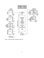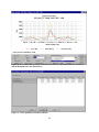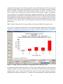
1
U.S. DEPARTMENT OF THE INTERIOR
U.S. GEOLOGICAL SURVEY
Evaluating Water Management Strategies with the Systems Impact Assessment Model:
SIAM Version 3
March 2003
by
John Bartholow1, John Heasley2, Blair Hanna2, Jeff Sandelin2, Marshall Flug1,
Sharon Campbel1l, Jim Henriksen1, and Aaron Douglas1
Open-File Report 03-82
This report is preliminary and has not been reviewed for conformity with U.S Geological Survey
editorial standards. Any use of trade, product, or firm names is for descriptive purposes only and
does not imply endorsement by the U.S. Government. Although the software referenced by this
report has been used by the U.S. Geological Survey, no warranty, expressed or implied, is made by
the USGS as to the accuracy and functioning of the software and related materials nor shall the fact
of distribution constitute any such warranty, and no responsibility is assumed by the USGS in
connection therewith.
1
Biological Resource Division
Fort Collins Science Center
Fort Collins, Colorado
2
Johnson Controls World Services
Fort Collins, Colorado
Suggested citation:
Bartholow, J.M., J. Heasley, R.B. Hanna, J. Sandelin, M. Flug, S. Campbell, J. Henriksen, and
A. Douglas. 2003. Evaluating Water Management Strategies with the Systems Impact
Assessment Model: SIAM Version 3. U.S. Geological Survey, Fort Collins Science
Center Open File Report 03-82. Fort Collins, Colorado. March 2003. 127 pp.
Available on the Internet at http://www.fort.usgs.gov
Preface
This booklet serves as an introduction to the SIAM, a System Impact Assessment Model for riverine
ecosystems. SIAM is an integrated set of models used to address significant interrelationships
among selected physical (temperature, microhabitat, and geomorphic features), chemical (dissolved
oxygen) and biological variables (young-of-year salmonid production), and stream flow in a river.
SIAM has been developed for the lower Klamath River from Klamath Falls, Oregon, to the river's
mouth on the California coast using data and models selected to be appropriate for the riverine
portion of that study area. SIAM is only as good as the data, models, and its users allow it to be.
This document highlights the important assumptions and limitations of these data and models so that
use may be enlightened as well as productive. We have tried to assure the quality of the data and
models integral to SIAM for the Klamath River; however, we stress that common sense may not be
left behind in applying SIAM for any specific analysis. Users must be vigilant in making sure that
the results logically follow from the premises. A warranty is neither stated nor implied.
SIAM represents only a small portion of any true ecosystem analysis and its results must be
considered in context with numerous other ecological, institutional, and political realities. SIAM is
not meant to be a decision-making device, but it is rather a decision aid. It is infeasible to model all
important resource impacts and impossible to anticipate all possible water supply situations.
Discretion and informed guidance will remain a necessary ingredient for appropriate SIAM use.
We (USGS) continue to provide training & support for SIAM in partnership with other users, in
particular the US Bureau of Reclamation and the US Fish & Wildlife Service. However, given the
nature of the decision-making structure evolving in the Klamath Basin, we are looking to all
interested parties to help shape SIAM, build credibility, and lend objectivity through continuous
application and monitoring. In effect, we welcome participation from everyone.
Please direct comments or questions to:
U.S. Geological Survey
Fort Collins Science Center
2150 Centre Avenue, Bldg C
Fort Collins, CO 80526-8118
970-226-9319
970-226-9230 fax
iii
Table of Contents
Forward ...................................................................................................................................... viii
Welcome..........................................................................................................................................1
Kick-starting SIAM .............................................................................................................1
What is SIAM? ....................................................................................................................1
SIAM for the Klamath River ...............................................................................................2
What's New About SIAM? ..................................................................................................4
Improving SIAM through Time...........................................................................................8
Acknowledgments................................................................................................................8
The Components of SIAM
The Water Quantity Component - MODSIM ....................................................................12
The Water Quality Component - HEC-5Q ........................................................................16
The Aquatic Habitat Component .......................................................................................23
The Anadromous Fish Production Component - SALMOD .............................................26
The Ecosystem Health Component - Red Flags ................................................................32
Tying the Components Together through Space and Time ...............................................34
Getting Underway........................................................................................................................38
Hardware & Software Requirements .................................................................................38
Installing SIAM on Your Computer ..................................................................................39
The Basics - What's SIAM's Main Screen .........................................................................40
Taking Shortcuts ....................................................................................................41
Getting Assistance while You Work .....................................................................41
A Guided Tour - Your First Evaluation.............................................................................41
Establishing a Baseline Alternative .......................................................................41
Making the Necessary Changes .............................................................................45
Running SIAM.......................................................................................................54
Looking at Results .................................................................................................55
Making Graphs Convey What You Want..............................................................56
Comparing Alternatives Graphically .....................................................................70
Generating An Alternative Comparison Report ....................................................73
Viewing Red Flag Results .....................................................................................75
Managing Your Alternatives .................................................................................77
Generating An Alternative Options Report ...........................................................78
Communicating Your Findings with Others..........................................................79
iv
Table of Contents (continued)
Advanced Topics ...............................................................................................................80
Adding Daily Variability to MODSIM Output......................................................80
Viewing Spatial Distribution of Temperature in SIAM ........................................85
Computing The Potential For Fish Kill In SIAM ..................................................87
Making "Management" Runs with MODSIM .......................................................88
Steps in Using SIAM .........................................................................................................97
SIAM Caveats .................................................................................................................100
Uninstalling SIAM...........................................................................................................102
To Learn More about SIAM.....................................................................................................103
Appendix 1.
Appendix 2.
Appendix 3.
Appendix 4.
Appendix 5.
Appendix 6.
Example Red Flag Criteria for SIAM ...................................................................107
Baseline Files Supplied with SIAM......................................................................111
Summer Maximum Daily Water Temperature Prediction ....................................112
Data Files Available for "Expert" Users ...............................................................115
Conducting a Microhabitat Time Series Analysis Using SIAM...........................116
Nutrient Loading Estimation Spreedsheet Model .................................................123
List of Figures
Figure 1. SIAM's Components......................................................................................................10
Figure 2. Important inputs and outputs for MODSIM..................................................................15
Figure 3a. Average measured and simulated mean daily water temperature for Seiad Valley
Gage location in the Klamath River from water years 1961 through 1999...................................18
Figure 3b. Comparison of simulated and measured mean daily dissolved oxygen concentration
at the Iron Gate Dam in the Klamath River from water years 1996 through 1999. ......................18
Figure 3c. Comparison of measured and simulated mean daily water temperature at the Seiad
Valley gage location in the Klamath River for two wet water years, 1965 and 1971. ..................19
Figure 3d. Comparison of measured and simulated mean daily water temperature at the Seiad
Valley gage location in the Klamath River for two dry water years, 1968 and 1977....................19
Figure 4. Important inputs and outputs for HEC-5Q. ...................................................................22
Figure 5. Major components of aquatic habitat analyses..............................................................25
Figure 6. SALMOD schematic. ....................................................................................................30
Figure 7. Important inputs and outputs for SALMOD. ................................................................31
Figure 8. Important inputs and outputs for Ecosystem Health component. .................................33
Figure 9. SIAM requires the Close on exit box to be checked in the MS-DOS Prompt and
Command.com properties window. ...............................................................................................39
Figure 10. SIAM's main menu showing map, toolbar, status bar, and tool tips. ..........................40
Figure 11. The New Alternative dialog with a name typed in and selections being made...........42
v
Figure 12. Selecting the folder in which to store your new alternatives. .....................................43
Figure 13. Completed File|New dialog.........................................................................................44
Figure 14. The Edit|Year dialog with three hydrologic years entered but all use the same
meteorologic year. Note that the user enters values in the first table only. The other tables are
for information only and are not editable. .....................................................................................45
Figure 15. The Edit|Node Criteria dialog. ....................................................................................47
Figure 16. Edit Node Priorities dialog showing the relative priority of each storage and demand
node. Note that the lower the priority, the more the water quantity model tries to meet the stated
target. .............................................................................................................................................49
Figure 17. Edit/Reservoir Characteristics dialog..........................................................................50
Figure 18. The Edit|Supplemental Fish dialog after entry of two groups of fish, juveniles in May
at week 32 and adults for the second year at week 54. .................................................................51
Figure 19. Red Flags dialog after a new red flag has been added. ...............................................53
Figure 20. Available output tables for the water quantity model. ................................................55
Figure 21. Exceedence plot for temperature at Iron Gate Dam. ...................................................58
Figure 22. Flow curves for the release from Iron Gate Dam, the Klamath below the Scott River,
and the Klamath below the Shasta River. ......................................................................................59
Figure 23. Water quantity model flow statistics. ..........................................................................59
Figure 24. Average mean daily temperature at Iron Gate and Keno dams...................................60
Figure 25. Annual cumulative temperature exposure at Iron Gate Dam. .....................................62
Figure 26. Exposure periods for Keno, Copco, and Iron Gate dams. ...........................................63
Figure 27. Area plot of thermal window for Iron Gate Dam at 15 ° C.........................................64
Figure 28. Temperature related macrohabitat...............................................................................64
Figure 29. Longitudinal profile for dissolved oxygen on June 1, 1993........................................65
Figure 30. Fish production graphics. ............................................................................................66
Figure 31. Add a curve dialog. .....................................................................................................66
Figure 32. Length frequency distribution for migrating Chinook Salmon pre-smolts. ................67
Figure 33. Mortality partitions for pre-smolts. .............................................................................68
Figure 34. Select mortality/life stage combinations by clicking on the check boxes...................69
Figure 35. Dialog for setting temporal limits and units................................................................69
Figure 36. Comparison alternative selection dialog .....................................................................71
Figure 37. Comparison of dissolved oxygen for two alternatives. ...............................................72
Figure 38. Comparison of discharge from Iron Gate Dam with historical data. ..........................72
Figure 39. Alternative selection dialog.........................................................................................73
Figure 40. Alternative comparison report parameters dialog box. ...............................................74
Figure 41. Dialog for editing a report name or deleting reports. .................................................75
Figure 42. Red Flag results for week's maximum temperatures greater than 16 °C.....................76
Figure 43. SIAM's Red Flag display for the item you added earlier. ...........................................76
Figure 44. Save As options............................................................................................................77
Figure 45. Dialog for saving as a new alternative. .......................................................................78
Figure 46. Iron Gate Daily Flow Variability dialog.. ...................................................................81
Figure 47. Yearly and monthly graphs of daily flows. .................................................................82
Figure 48. Daily patterns constructed from months listed in Table 7...........................................84
Figure 49. Iron Gate Daily Flow Pattern Template Dialog. .......................................................85
vi
Figure 50. Spatial distribution dialog for temperature on June 1, 1993. ......................................86
Figure 51. Dialog for generating potential for fish kill data. .......................................................88
Figure 52. Plot of Hydrologic State "Factors" for Upper Klamath Lake (Link Dam)..................90
Figure 53. Plot of Reservoir Target Values for Three Hydrologic States at Link Dam.
Figure 54.
Figure 55.
Figure 56.
Figure 57.
Figure 58.
Figure 59.
Figure 60.
Figure 61.
Figure 62.
Figure 63.
Figure 64.
Figure 65.
Figure 66.
95
Plot of Reservoir Target Values for Three Hydrologic States, Iron Gate. ..................96
Uninstalling SIAM from your computer. ..................................................................102
Example maximum temperature prediction for Seiad...............................................113
Selecting a single hydrologic water year for a SIAM run.........................................117
Selecting Fish Production Comparative Graphs in the SIAM main window............118
Alternative comparison graph options to compare two or more years......................118
Selecting an alternative year for comparison ............................................................119
Setting the temporal limits appropriate for a specific life stage................................120
Microhabitat output for fry, WY1982 and WY1994, adjusted for time present .......121
Curve statistics for the graph shown in Figure 61.....................................................122
Excel macro query and selection menu. ....................................................................123
Alternative worksheet for nutrient loading estimation model...................................124
Chart worksheet in the nutrient loading estimation model........................................125
List of Tables
Table 1. SIAM's Attributes ..........................................................................................................11
Table 2. Differences in MODSIM prediction and gaged flows. Adapted from Campbell et al.
(2001). 14
Table 3. Water quality error and correlation statistics..................................................................17
Table 4. Example life stage and class structure definition of an anadromous salmonid population
along with the model's order of calculation. Classes are defined by percent development
(deposition to emergence) for egg stage and by length (mm) for fry to yearling..........................29
Table 5a. Approximate crosswalk between SIAM component model's spatial representations for
the with- and without-Project network (#1) down to Seiad, California. The without-Project
network (#2) extends the HEC-5Q network upstream to Upper Klamath Lake and differs in the
exact location of Control Points 10 and 15. .................................................................................35
Table 5b. Continuation of Table 5a for segments downstream from Seiad, California (Network
3) to the ocean. Note that SALMOD does not extend below the Scott River. .............................36
Table 6. Approximate crosswalk between SIAM component models' temporal representations.37
Table 7. Years chosen to represent Iron Gate Dam discharge by month and exceedence level...83
Table 8. Hydrologic state factors..................................................................................................90
Table 9. Primary reservoir targets.................................................................................................91
Table 10. Secondary (smaller) reservoir targets. ..........................................................................92
vii
Forward
Water from many of California's coastal rivers has been used for a wide variety of development
ventures, including major agricultural diversions, hydropower generation, and contaminant
assimilation from industry, agriculture and logging. Anthropogenic impacts often degrade water
quality and decrease the quantity and quality of aquatic habitat. Reallocating streamflow away from
uses that degrade water quality to uses that foster higher water quality is a critical step in restoring
riverine habitat and the anadromous fish that rely on that habitat for a portion of their life cycle.
Reallocation always brings with it the need to examine the economic efficiency of the proposed
changes. If the dollar benefits of improving water quality are greater than the costs, the criterion of
improving economic efficiency is satisfied, a fact that can be highly persuasive to decision makers
contemplating reallocation.
Previous related studies have examined nonmarket benefits of the Trinity River in northern
California (Douglas and Taylor, 1998; Douglas and Taylor, 1999abc) but nothing of this kind had
been done on the Klamath River, another system with numerous uses for and competition over water
in times of drought. An economic survey is nearing completion for the lower Klamath River,
including the Scott, Shasta, and Salmon Rivers, but excluding the Trinity. This survey provides
valuable insights about the magnitude of the benefits and nature of the costs of reallocating water
from market uses to instream flows that improve water quality and assist in the recovery of Klamath
River fish stocks.
Preliminary survey results (Douglas and Johnson, 2002.; Douglas and Sleeper, In Prep.) indicate that
about 234,000 California, Oregon, and Nevada households made recreation trips to the lower
Klamath River Basin 1997-1998 and that these users spent about $780 million on trip related
expenditures. Clearly the prosperity of the region is closely linked to the demand for Lower
Klamath River Basin recreation trips. Further, respondents indicated that they would make roughly
36% more recreational trips per annum to the Klamath if the water quality and the fishery were
restored to an unspoiled condition. Using two distinct types of survey data, these additional trips
would yield benefits with a present value of approximately $20 billion (at a discount rate of 7.5%).
Calculating costs to restore the fishery and raise water quality involved five major hypothetical
restoration activities: (1) purchasing Klamath project farmland and environmentally sensitive forest
lands, (2) allocating more water down the Trinity River to enhance the quantity and quality of
Klamath flows below the confluence, (3) removing four mainstem dams along the Klamath River
and losing their associated hydropower production, (4) eliminating all harvest of Klamath-Trinity
fish stocks for a 12-year period including the acquisition of fishing rights from both tribal and
commercial marine fishermen, and (5) operating all Klamath-Trinity fish hatcheries to restore selfreproducing stocks. In total, restoration costs were calculated to be about $5 billion. If the
assumptions used in this study are valid, it is clear that the baseline benefits ($20B) far outweigh the
costs of restoring water quality and the fishery.
The apparent disparity between restoration benefits and costs for the lower Klamath River may
suggest to some that water resources on the Klamath be reallocated to environmentally friendly
viii
nonmarket uses. The economic analysis rests in part on the information made available to the survey
designers by the biological, hydrologic, and water quality data incorporated in The System Impact
Assessment Model (SIAM). It is our hope that SIAM can be used to improve the river's water
quality and fishery, and strengthen the important regional economy.
ix
Welcome
Kick-starting SIAM
If you are anxious to install SIAM and give it a trial run, you may safely skip ahead to the 'Getting
Underway' chapter of this document and do just that. However, if you have a previous version of
SIAM installed on your computer, please uninstall it completely before installing this version. After
installation, it would be wise to re-run any alternatives you wish to retain. Then do come back to
review the background and components of SIAM, as they are important in any informed use of this
software and its models; to do otherwise would be negligent.
What is SIAM?
The System Impact Assessment Model, SIAM, is an integrated set of models and data assembled to
evaluate and compare the potential impacts of water management alternatives from an ecological
perspective. SIAM's goal is to further the process of reaching a decisive consensus on management
of water resources in order to stabilize and restore riverine ecosystems, and is meant to be used in
the context of the Instream Flow Incremental Methodology (IFIM) as summarized by Stalnaker et al.
(1995). To achieve this goal, SIAM must help quantify consequences of water management
alternatives in terms of the major physical, chemical, and biological indicators known or strongly
believed to be intimately related to the success of anadromous fish restoration. For our purposes,
water management may be defined as direct or indirect control of the quality, magnitude, duration,
frequency, timing, or rate of change in river flows under man's influence.
SIAM is primarily intended for planning and management as opposed to research; SIAM is not
meant to supply the answer. Management models integrate the best available knowledge to provide
managers with the predicted results of potential actions (i.e., a what-if model). SIAM may be used
also in a planning mode by portraying the simulated effects of actions against a long-term historical
backdrop. Planning models are descriptive, fostering the development of robust and non-arbitrary
policies on which all water users may rely. In contrast, operational models are prescriptive, used
primarily to fine tune near-future actions. We recognize that some components of SIAM may indeed
be useful in guiding day-to-day or month-to-month operational decisions, but that was not its
designed purpose.
SIAM provides the framework for a general purpose modeling environment in the sense of coupling
models and data in a manner appropriate for specific applications. The keys to a general purpose
modeling environment are that 1) the component models and data are independent yet integrated, 2)
outputs are hierarchical, 3) individual components are credible, and 4) all parties are quite clear
about what the model(s) will and will not do. Independence in this context means that the models
are modular and usable on their own. Some applications need not employ the full set of capabilities
of all models. Users from specific disciplines will want to concentrate on specific submodels.
1
Being modular also implies that models are portable and can be interchanged when obsolete or in
need of refinement. Integrated means that the independent models must be "harmonized" in a
relatively transparent manner to form the whole suite. In general terms, the water quantity model is
the fundamental driver, the entrée for all subsequent models, and serves as a shared resource and
core database -- the integrator. In another sense however, integrated also means the user interface,
which is the "front end" – this is SIAM.
Hierarchical outputs means three things. It means that the user can look at output 1) at a single
location or aggregated through space, and 2) at a single time or aggregated through time. It also
means that there are enough detailed outputs that the user can trace a "high level" output back
through the simulation results that comprise that aggregate. For example, if a user is interested in
the number of outmigrating fish, she or he can see why that number changed in one scenario versus
another, i.e., trace the result back to water quality, then to temperature, then to streamflow, then to
the meteorology of a hot day. Hierarchical output also facilitates dealing with "hierarchical users".
That is, users with a policy focus can deal with aggregated responses while technical users can deal
with the more detailed elements.
Credible means several things. It means that the component models are testable, that they are
scientifically up-to-snuff (if not state-of-the-art), and that they are peer reviewed. Credible means
that the components are detailed enough to give the spatial and temporal resolution required to meet
the objectives satisfactorily, but simple enough to understand and satisfy the goal of parsimony. If
too complex, models consume precious resources and computing power. Credible means that the
simulations operate with a level of realism (agreement with intuitive or testable perceptions) and
precision (close-enough agreement with measurements) to be persuasive. Credible also means that
assumptions and limitations of the components are clearly stated, and that care is taken to prevent
misuse beyond their inherent regions of predictive extrapolation.
SIAM for the Klamath River
If SIAM remained merely a concept it would serve no useful purpose. This version of SIAM is
targeted for a portion of the mainstem Klamath River from Upper Klamath Lake, Oregon, to the
Pacific ocean. Important metrics for this evaluation include water quantity, water quality, fish
habitat, fish production, and other measures of 'ecosystem health.' Consequently, models and data
dealing with these elements and focused on the Klamath River form the core elements for SIAM.
SIAM starts with a water quantity model, MODSIM (Fredericks and Labadie, 1995), to predict river
flows and track reservoir volumes in the Klamath River system including the U.S. Bureau of
Reclamation's Klamath Project and downstream through the reservoir complex managed by
PacifiCorp. MODSIM employs a prioritization scheme to model flows throughout this system under
different water management alternatives consisting of reservoir operating "rules" and constraints,
instream flow requirements, agricultural demands, and water allocations. MODSIM can also track
power generation at reservoir power plants, though SIAM does not make these results available at
present.
2
Flows simulated by MODSIM are next passed to a Corps of Engineers-developed water quality
model, HEC-5Q (USACOE, 1986), to predict selected water quality constituents throughout the
river. For the Klamath River, the constituents simulated are water temperature, dissolved oxygen,
and conductivity.
Aquatic habitat is a general term that refers to any part of a stream where an aquatic organism lives.
Aquatic habitat is dependent on both water quantity and quality, the determinants of micro and
macro habitat combined to give total habitat. Aquatic habitat has been characterized in SIAM using
elements from the Physical Habitat Simulation System, PHABSIM (Milhous et al. 1989; USGS
2001), and from the Time Series Library (TSLIB) as described Milhous et al. (1990). Important
habitat elements include water depth, velocity, substrate, and cover. In addition, channel
morphology, sediment budget, and thermal refugia are relevant macrohabitat features, but not
adequately addressed in SIAM at present. Quantification metrics include duration, frequency,
magnitude, and rate of change of integrated measures of total habitat. Strictly speaking, PHABSIM
is not a functional component of SIAM in the same way as the other models. This is because it has
been run independently to generate a portion of the data made available to SIAM; these data are used
primarily in a fish production submodel, SALMOD.
Fish production is dependent on the time series of micro and macro aquatic habitat, as well as the
number of adult spawners present. SIAM employs a fish production model, SALMOD (Williamson
et al., 1993; Bartholow et al., 1993), to track the relative number and weight of juvenile chinook
salmon successfully exiting the study area. It also identifies the relative magnitude of various
sources of mortality, including water temperature, movement, and nesting superimposition,
throughout the early life history of the species under consideration. All mortality sources are
ultimately traceable back to water quantity and quality variations over time.
Collectively, all of SIAM's output metrics are used to characterize ecosystem health. Though not
represented by a single numeric quantity, ecosystem health in the context of SIAM is embodied in
the output by the number of occurrences of various metrics falling outside of user-prescribed
bounds, and the physical extent of those deviations. For example, dissolved oxygen falling below
5.0 mg/l on a daily basis would be "flagged" as unacceptable. In fact, SIAM's presentation for
ecosystem health is a set of so-called Red Flag displays that capture the encroachment of standards
through time and space. These Red Flags are supplemented by a set of powerful water quality
metrics, such as degree-days.
Binding the models, data, and simulation results is the user interface for SIAM which tracks the
options that the user wants to simulate, passes data and simulation results as necessary to the
appropriate models, and summarizes the output for convenient display. We have termed this overall
component "Cross-Talk" for convenience, even though there is no software with this specific name
for SIAM. Cross-Talk is responsible for the almost endless bookkeeping that is required to link
models together that may have different spatial and temporal scales (months, days, weeks), different
input and output units (feet, meters), and different computer file formats - no small task.
3
We will have more to say about each of the major subcomponents in the remainder of this document.
For the present, it is necessary simply to introduce a few modeling terms that may be useful in
understanding SIAM. Calibration means using measured or observed input and output information
to adjust or estimate parameters so the model's predications match empirical observations.
Reference or Baseline Condition refers to those conditions occurring during the reference time
frame, usually referring to water supply, habitat values, or population status. The reference
condition is often an actual recent historical condition, but may also represent: (1) the same
climatological-meteorological conditions but with present-level water development and operations;
(2) the same climatological-meteorological conditions but with both current and proposed future
development on line; and/or (3) some estimate of virgin or pre-development conditions. Validation
means determining how accurately the model can predict conditions different from what was used to
develop and calibrate the model. Contrast this with verification by which we mean only assuring
that a computer program functions or makes its calculations as intended.
SIAM for the Klamath is a medium resolution model through time and space. That is, river flows
and related elements range from monthly to daily in the temporal domain and are rarely truly
continuous through space. It is anticipated that SIAM will not fully answer all detailed questions if
the spatial or temporal scales necessary are finer than this. Other models could of course be added to
SIAM as discussed previously. However, in many or most cases a better strategy may be to have
SIAM help focus a more intensive analysis. For example, diurnal dissolved oxygen swings are
thought to be important in the Klamath. However, it is likely that only certain times of the year are
critical. SIAM may be used to identify those critical times of the year or river segments under a
variety of water management scenarios to be examined in more detail with techniques appropriate to
the questions being asked. For dissolved oxygen, this may involve a more detailed hydrodynamic
model, such as is being applied by the University of California, Davis (Deas and Orlob, 1999), or a
relatively sophisticated regression model.
What's New About SIAM?
Version 3.0 (January 2002) added target matching tables to the water quantity output tables. The
SIAM Help was replaced by extensive context sensitive help. A new splash screen was added for
version 3.0, along with numerous other minor enhancements. Version 3.4 contains bug fixes to
several items, especially Red Flags, and adds fish mortality partitions to the graphing options and a
Delete Alternative feature to the File menu. Importantly, SIAM now supports only two networks,
Upper Klamath Lake to the ocean either with or without project. By project, we mean the series of
reservoirs below Upper Klamath Lake that are managed by PacifiCorps. (Though you will find
reference to other networks in this documentation, these references were retained for historical
purposes only.) There were also minor changes to MODSIM's data files. Version 3.6 added the
capability to compute potential for fish kill based on ammonia concentrations, pH, and temperature.
We also added two more years (2000 and 2001) to the historical database and added a nutrient
loading spreadsheet model supplement (Appendix 6).
4
Version 2.9 (November 2001) added a spatial display module to SIAM. This module shows the
spatial distribution of temperature, dissolved oxygen, and discharge over the length of the Klamath
River. This display can be animated over time. The capability to display temperature in Fahrenheit
degrees was added to SIAM's graphic displays. The DOS version of SALMOD has been replaced
with a Windows version and the SALMOD graphics were updated within SIAM. SIAM now has the
capability to also run the stand-alone version of SALMOD. The SIAM toolbar has been redesigned
and new buttons were added. SIAM output additions include an alternative options report and a
target matching table. Water surface elevation has been added to the red flag criteria.
Version 2.7 (May 2001; Version 2.6 was solely an experimental release) allows a much finer
prediction of the water surface elevation for each reservoir, especially Upper Klamath Lake. This
version allows one to set minimum and maximum reservoir storage volumes and monthly targets as
either water surface elevations (feet above mean sea level) or volumes (acre feet). This was
accomplished by including a detailed storage-elevation-surface area table and a revised verification
of the water quantity model to reflect the Bureau of Reclamation's current best estimate of Upper
Klamath Lake's bathymetry and total storage of the lake rather than just active storage as had been
previously modeled. Version 2.7 also contains the ability to superimpose a daily release schedule
from Iron Gate Reservoir such that the influence of daily variability may be reflected in the water
quality and fish production models' results. Minor changes to river mile designations were made to
Version 2.7.
In adding the lake level features, several potential inconsistencies were identified. It may be
instructive to mention them as they shed light on the sometimes mysterious world of modeling. First,
we found that MODSIM's method of accounting for evaporation was unexpected. Basically, the
water quantity model subtracts monthly evaporation after all other constraints have been met. This
meant that, although MODSIM accounted for the minimum possible volume as specified in the node
characteristics, the end-of-month storage passed to SIAM (and therefore HEC-5Q) could be lower
than that minimum, causing problems in the water quality model.
Second, we found that the available reservoir bathymetry estimates for Upper Klamath Lake had
problems. Depending on the source of the tables (both storage-elevation and storage-area), the
values may or may not agree. This was traced in part to revisions to the bathymetry given new
hydrographic surveys and alterations in the benchmark elevations. In addition, sometimes the units
of the table were unclear; the values may have been total storage, or just "active" storage (i.e., only
usable water above the inactive or dead pool.) Thus, the datums for minima and maxima are
somewhat fuzzy, especially for Upper Klamath Lake. We have elected to standardize on the data set
inherent in KPOPSIM as downloaded from the Bureau web site (http://www.mp.usbr.gov/kbao).
A related issue is that the historical reservoir storage volumes reported by the Bureau of
Reclamation and PacifiCorp occasionally were either higher or lower than the stated maxima or
minima, implying gauging error, large seiching of the reservoir pool, or other unspecified problems.
Since MODSIM was calibrated to the reported storage values, it only makes sense that the
respective minima and maxima allow for reasonable deviations from the published values.
5
We (USGS) have made what we hope are reasonable compromises in putting in our best
understanding of the actual storage-elevation-area tables, as well as good estimates of reservoir
storage minima and maxima. These limit values were chosen to represent the existing plumbing
(e.g., the sill elevation for Upper Klamath Lake and elevations of current reservoir outlets), taking
MODSIM's evaporation into account, and pretty much ensuring that the water quality model is
stable for the calibration runs. Both MODSIM and HEC-5Q only use a subset of the total number of
points on the non-linear storage-elevation curves; therefore the resulting piecewise linear
interpolation estimates may contain some discrepancies from the complete tables of curve numbers
available. In turn, SIAM "knows" these tables (curves) extrapolated to include storage values both
higher and lower than have ever been recorded. This is to allow exploration of potentially
reasonable water management alternatives like lowering the UKL sill or raising the height of various
dams in a "what-if" fashion.
Providing the freedom to experiment also has its risks. For example, reducing reservoir storage to a
very small value and then subjecting it to high flow events may seriously violate HEC-5Q's
minimum retention time limits ([reservoir volume/max(Qin,Qout)]<1 day) resulting in either
unrealistically poor water quality (e.g., water temperatures > 50°C) or complete model failure.
Luckily, these conditions are easy to spot as errors. Unfortunately, it may also be possible to
generate sets of conditions that cause the model to give poor predictions, but the user may not know
it. All we can say is that as you push these models farther from the domain for which they were
calibrated, you increase the likelihood of encountering problems.
The complete storage-area-elevation tables for Upper Klamath Lake, Lake Ewauna, Keno, JC Boyle,
Copco Lake, Copco 2, and Iron Gate have been provided with the SIAM Version 2.7 software. In
order to provide flexibility for "what-if" simulations, the maximum capacities of Upper Klamath
Lake, Copco Lake, and Iron Gate have been increased. To achieve this objective, the storage-areaelevation tables have been extrapolated above the previously available maximum reservoir levels as
mentioned above. These files are named like UKL_SAE_Table.dat, with similar names for the other
reservoirs, are stored in the SIAM install directory and may be easily read. Note that Lake Ewauna,
JC Boyle, and Copco 2 are not simulated in HEC-5Q.
The Klamath_to_the_ocean_61-99.XY and Management-All.XY files have changed with SIAM
Version 2.7. New XY files (with a –C.XY suffix) have been included that reflect the extrapolated
Upper Klamath Lake, Copco, and Iron Gate storage-elevation-area values. If the user wishes to
simulate larger reservoirs for "what-if" alternatives, the –C.XY files should be used.
Version 2.7 also adds the capability to generate alternative comparison reports. Differences above
specified thresholds for water quantity model discharge and storage and water quality model
discharge, temperature, dissolved oxygen, storage, water surface elevation, and conductivity can be
reported.
Version 2.5 (March 2001) added a matrix of historical flows to aid in the selection of comparable
years to evaluate. SIAM can now set reservoir storage targets in terms of water surface elevations as
well as volumes. This is important for consideration of lake levels mandated for endangered lake
6
sucker protection. Some of the MODSIM data files have been updated with more accurate data or
parameter values. As always, numerous small bugs were found and corrected. NOTE: it would be
best to rerun any previous versions of SIAM alternatives since this new software may not be able to
process previous results correctly in all circumstances.
Versions 2.3 and 2.4 (January 2001) added the capability to superimpose daily flow variability on
the monthly output from the MODSIM model downstream from Iron Gate dam. This should provide
more realistic estimates of the variability of downstream water quality results, and allow for the
evaluation of "split-month" flow schedules. An exceedence plot function was added to most of the
graphic output for SIAM. You can also set the Y-axis extents for all graphic output.
Version 2.2 (November 2000) extended the Klamath network downstream from Seiad Valley,
California to the ocean, and upstream to Upper Klamath Lake. The user interface has been
redesigned to improve ease of use, flexibility, and utility. All new graphics output for water
quantity, water quality, and fish production has been incorporated into SIAM. Five new water
quality metrics have been added. These include: annual exposure to temperature and dissolved
oxygen, exposure period, thermal window, macrohabitat, and longitudinal temperature, discharge,
and dissolved oxygen profiles. All output graphics can be exported to files that can be read by MS
Excel, adding even more flexibility and utility to the software. Additional control over MODSIM
has been afforded through the ability to specify maximum flows as well as minimum flows.
Comparison of alternatives may now be made graphically. A statistics option has been added to all
output graphics, providing standard descriptive statistics. Finally, a preferences dialog has been
added to streamline color selection for graphs and facilitate disk file management.
Version 1.3 (January, 2000) added the ability to work with different networks. For the Klamath in
particular, the existing, with-project network (#1) was supplemented with a without-project network
(#2) containing no reservoirs on the mainstem Klamath below Upper Klamath Lake. This change
also allows us to have the network that simulates from Upper Klamath Lake to the ocean (#3), which
is available with Version 2 of SIAM. Each unique network has data files specific for it, particularly
the so-called .XY files for MODSIM. Version 1.3 also upgraded the graphics to more correctly
handle the output from HEC-5Q and added output in the form of .CSV files that are more easily
imported into Microsoft Excel. Finally, error processing is more robust.
Version 1.2 (December, 1999) added the ability to run SIAM for up to 50 contiguous years. For the
Klamath River, meteorological data were supplied for WY1961 to 1997, as well as three synthetic
years: Hot, Cold, and Median. Fill and Clear buttons were added to the Edit|Year dialog to facilitate
running such a long data set. Note that if more than five years are run in sequence, the fish
production model, SALMOD, does not produce a full complement of output. Version 1.2 also
distributed a more realistic starting set of Red Flag values.
Version 1.1 (October, 1999) added many improvements to the prototype release (October, 1998).
Major changes include:
• SIAM now can run and display up to five years worth of simulation at one time. The user
has control of which hydrologic and meteorological years to simulate, in any order desired.
7
•
•
More flexibility in controlling a MODSIM "management" style simulation run. This allows
for different rules to be applied in dry, average, & wet months.
Consolidated entry of information to create and store New alternatives.
Improving SIAM through Time
It is our intention to continually improve SIAM and it's component models. We always have a list of
capabilities and data that we'd like to add to SIAM. In addition, there is no way that this version of
SIAM is completely bug free. Please direct all suggestions for product improvement to the USGS at
the address given above.
Acknowledgments
We gratefully acknowledge the feedback provided by R2 Resource Consultants, Inc., of Redmond,
Washington, in their review (1997) of the prototype SIAM as presented at a workshop in August
1997. R2's descriptive summary was useful in helping us see SIAM from the perspective of
someone not intimately involved in its development. In fact, we have adapted their summary for
some of the introductory material in this manual. Their review also helped us understand what to
stress or revise to correct some misunderstandings of both fact and interpretation. In addition,
material from other sources was instrumental in shaping the philosophy of SIAM. See the citations
in the references section for these sources.
Several individuals from the US Bureau of Reclamation have helped shape SIAM (whether they
knew it or not). Larry Dugan, Klamath Basin Area Office, generously helped underwrite
improvements for Versions 1.2 and 1.3. Leon Basdekas in the same office (and now with Utah State
University along with Matt Combes) asked critical questions helping to improve SIAM's interface
with other models such as KPOPSIM. Nancy Parker, Ken Mangelson, and Ron Sutton, Denver
Regional Office, helped with product development and suggestions for application improvements.
In addition, staff from the US Fish and Wildlife Service have been instrumental in testing and
shaping SIAM. Tom Shaw, Charlie Chamberlain, Paul Zedonis, and George Gullien have made
significant contributions to SIAM.
Other members of the USGS Klamath River study team, including Clair Stalnaker and Sam
Williamson, all served as extensive advisors in the construction of SIAM. Jeff Sandelin artfully
engineered the first versions of the SIAM user interface. John Scott, Steve Witter, and Catherine
"Cat" Shrier have made MODSIM a great tool for the Klamath. Mark Baldo helped with MODSIM
technical issues. Graphics assistance was provided by Jennifer Shoemaker and her staff.
8
Figure 1. SIAM's Components
Data
Requirements
and more . . .
Functional Models and Routines
Water Quantity Model - MODSIM
Σ Developed at Colorado State University
Σ Allows generation of monthly flow alternatives
throughout the network
Σ Calibrated for 1961-1997 period
Σ Flows in acre-feet per month
Σ Tracks reservoir storage and capacities
Σ Application user and peer reviewed under FWS
contract
Water Quality Model - HEC-5Q
Σ Developed by US Army Corps of Engineers
Σ Calculates longitudinal water temperature and
other water quality parameters from daily
flows, and meteorology
Σ Includes in-reservoir water quality effects
Σ Calibrated for 1996; validated for 1997
Aquatic Habitat Models - As Input to Other Models
Σ Developed by USGS (formerly FWS)
Σ Estimates quantity and quality of habitat
Σ Requires channel geometry and more
Σ Peer and user review has been extensive
Anadromous Fish Production Model - SALMOD
Σ Developed by USGS (formerly FWS)
Σ Estimates outmigrating young-of-year fall chinook
from weekly flows, temperatures, aquatic habitat and
life history data
Σ Published in refereed scientific literature
Ecosystem Health Component - Red Flags
Σ Internal to SIAM
Σ Highlights when user-defined criteria have been
exceeded through space and time
Linkages - CrossTalk
Σ Internal to SIAM; Converts monthly flows into daily
and weekly patterns
Σ Will use daily accretions from Phase I analysis
Σ Sets up input files for communication between
models in terms of data units and format
Σ Presents limited model input for editing and
displays limited model output for analysis
Σ To be reviewed by repeated testing
9
Table 1. SIAM's Attributes
LIMITATIONS
- Each component model has inherent
uncertainty.
- Fall chinook only; no hatchery
component.
- Not all features of the final product are
available. In particular, geomorphology
and refugia are not yet represented.
- Evaluation of results is left to the user.
- The methodology governs the kinds of
questions that are asked, i.e., SIAM leaves
out non-habitat biological issues, e.g.,
exotics, disease, genetics, which may be
important.
ASSUMPTIONS
- A model is an abstraction and
simplification of reality.
- Reasonably represents the major limiting
habitat factors whose modification is
necessary to recover natural-reared
anadromous salmonids in the mainstem
Klamath.
- All of the component models, especially
fish production, have fundamental
assumptions.
- Assumes that actual operations can
closely mimic simulated operations.
- Assumes a "caretaker" to update the
model and become an "expert" user.
- Assumes that errors do not escalate from
one model to another.
STRENGTHS
- Integrates physical, chemical, and biotic
components of ecosystem using
sophisticated, yet modular routines.
- Provides quick insight into what is and is
not possible for resource management
- Handles all units' conversion and file
formatting to interweave models.
- Insulates the "casual" user from
component model complexity and
terminology.
WEAKNESSES
- Makes it so simple to run that some users
may not fully realize inherent limitations.
- Not all features of component models are
available for editing within SIAM.
- Documentation is always incomplete.
- Data for validation of component models
are limited. HEC-5Q is calibrated for
only two years, and SALMOD has not yet
been fully calibrated for the Klamath
River.
10
The Water Quantity Component - MODSIM
SIAM's water quantity model, called MODSIM, was developed at Colorado State University.
MODSIM is a network based water allocation planning model, which means that its specialty is the
analysis of water systems with numerous diversions, returns, and reservoirs in an interconnected and
managed system. Careful applications generate useful information about which, when, and how
fully water allocations are satisfied or not satisfied under a variety of water supply and system
operation policies for river basins. In short, MODSIM allocates water in a manner consistent with
the hydrological, physical, and institutional aspects of a river basin.
MODSIM simulates several types of water allocations, including:
•
•
•
•
•
Direct flow allocations (including conditional allocations)
Instream flow allocations
Reservoir storage allocations
Reservoir system operations
Exchanges and operational priorities (e.g., augmentation, subordination)
MODSIM offers a number of unique features, though SIAM does not make use of them all at this
time. They include:
• the ability to operate in monthly, weekly, or daily time steps through appropriate input data
preparation. For SIAM on the Klamath River, MODSIM has been applied using a monthly
time step. For more on how MODSIM's time step relates to that of the other models in
SIAM, please refer to Table 6.
• the ability to incorporate complex institutional and legal structures governing water
allocation in a basin, including complex exchanges and operating policies.
• relies on user input data, not a priori defined operating policies, to describe system features
and operational requirements separate from the network modeling algorithmic structure.
• capable of modeling looped and bifurcating water system features, and is not limited to
branching or treelike network structures.
• accurate calculation of system losses as a function of averaged flows and storage, such as
evaporation loss, channel loss, reservoir seepage and losses in water application.
• a graphical user interface (GUI) for drawing and editing system features, as well as a
spreadsheet-style data editing capability emulating a data-centered information system.
• hydrologic streamflow routing capabilities for daily simulation.
• utilization of a network flow optimization algorithm based on Lagrangian relaxation.
• accurate calculation of hydropower generation capacity and energy production based on
power plant efficiencies which can vary with flow, head, and load factor; calculates peak vs.
non-peak and firm vs. secondary energy production.
MODSIM is split into two functional pieces, a graphical user interface (GUI) to ease river network
creation, and the water allocation network solver. One of the strengths and relatively unique
11
features of MODSIM is its internal solution technique for system/priority optimization (Fredericks,
1993; Labadie, 1988). Luckily, SIAM users need to understand the solver only enough to try
different demand priorities and operations rules, explained later.
MODSIM represents the physical river system as a series of nodes and links. Nodes represent both
storage and non-storage aspects of a river system such as reservoirs, demand/diversion structures,
inflow locations, and stream gage locations. Links represent stream reaches, canals, tunnels, and
other methods of water conveyance. The basic nodal features of any water resources planning model
include reservoirs, diversion structures (demands), and inflow locations. A crosswalk between
MODSIM's network structure and that of the other models in SIAM for the Klamath River may be
found in Table 5.
An important assumption inherent in MODSIM's application for the Klamath River is that the time
step for the calibrated 1961 to 1999 period is monthly. In most cases, discharge from Iron Gate
Reservoir may be satisfactorily represented by monthly flows for two reasons. First, the Federal
Energy and Regulatory Commission's imposition of minimum flows for Iron Gate adhere to a
monthly timetable; also, reservoir storage levels in Upper Klamath Lake for the endangered sucker
adhere to monthly guidelines. Thus flows are, especially during the low flow portion of the
hydrologic year, fairly stable. Second, the nature of the basin's (mostly agricultural) water demands
and system of reservoirs also tends to stabilize the mainstem's flow regime. However, it is also true
that the system-wide storage is insufficient in most years to contain large runoff events and the
downstream tributaries remain largely unregulated and are therefore subject to peak events much
shorter than a month. Users of SIAM for the Klamath must remember these limitations, but recent
upgrades to SIAM allow more creative ways to deal with mid-month or daily flow variability.
For our purposes, MODSIM simulates several types of water allocations including direct flow
allocations, instream flow allocations, reservoir storage allocations, reservoir system operations,
exchanges and operational priorities (e.g., augmentation, subordination). Water is allocated to each
of these uses based on a user assigned priority for the link connecting the allocation to the river
system.
Priorities are ranked from low to high with the lower number representing the higher priority, i.e
satisfied first. MODSIM can handle multiple sets of priorities in its "management mode". In this
mode, the model chooses which set of priorities to use based on a monthly determination of
"hydrologic state". The state is defined in increasingly wet states as dry, average, or wet based on
the initial volume of user-specified reservoirs. In this way, one can have a variable "rule book" for
system management. Note: Although SIAM is currently limited to handling three hydrologic states,
newer versions of MODSIM can handle up to seven. If SIAM encounters a MODSIM management
XY file with other than three states, SIAM will still function properly, but only the expert user can
deal with such a file. See the MODSIM documentation and the section on Advanced Topics later in
this documentation for more information on how to set up and use a management run.
MODSIM has been calibrated for the Klamath River. Results from that calibration are summarized
below in Table 2. These figures represent a trivial percentage difference from USGS gaged flows
12
(on the order of 2 cfs on average). The maximum monthly differences are large, but represent onetime deviations due to a change in the operation of the upper basin reservoirs not captured by
MODSIM.
Table 2. Differences in MODSIM Prediction and Gaged Flows. Adapted from Campbell et al.
(2001).
USGS Gage
Location
Average Year Difference (m3 x 106)
Maximum Month Difference (m3 x 106)
Calibration
Validation
Calibration
Validation
Keno
1.7
1.9
1.4
146
Iron Gate
1.9
1.7
1.4
143
Seiad Valley
2.3
2.6
3.4
143
13
Figure 2. Important inputs and outputs for MODSIM.
The user is referred to the complete on-line help for MODSIM for more information on using its
standalone features that are not incorporated into SIAM.
14
The Water Quality Component - HEC-5Q
The water quality portion of SIAM for the Klamath River is filled by HEC-5Q. This model was
developed by the U.S. Army Corps of Engineers at the Hydrologic Engineering Center at Davis,
California (USACOE, 1986). HEC-5Q simulates the sequential operation of a reservoir system to
evaluate the operational "rules" for flood control and conservation (i.e., instream flow) purposes.
Water quality analyses include water temperature, three conservative and three non-conservative
constituents, and a dissolved oxygen/nutrient/phytoplankton option. Reservoir releases may be
computed to satisfy multiple control point (node) criteria using a philosophy of minimizing
"violations" of control point water quality requirements. HEC-5Q has some capability to simulate
multilevel reservoir withdrawal to accomplish downstream water quality objectives. Twenty
reservoirs, forty control points, and almost any length of study period can be simulated on an hourly,
daily, or monthly time interval. The model has a long history of supported use and is in the public
domain. HEC-5Q is one of a very few models that have been used for simulating both rivers and
reservoirs.
For the Klamath, only selected features of HEC-5Q have been implemented. None of HEC-5Q's
water quantity capabilities have been used; SIAM uses MODSIM for these. The water quality
portion of the model has been set up for mean daily simulation from Upper Klamath Lake
downstream using flow "demands" and reservoir storage imposed by the water quantity model,
MODSIM. The quantity model's mean monthly flow pattern is disaggregated into 30 days (or 28 or
31 as necessary) of equal daily average flow. (Note that you may provide daily flow patterns for
SIAM if desired.) In addition to Upper Klamath Lake, Keno, Copco, and Iron Gate reservoirs are
modeled, along with all major tributary creeks and rivers (e.g., the Shasta and Scott). Small
tributaries and undistributed inflows are also modeled solely as accretions. JC Boyle was simplified
due to model constraints. In addition to water temperature, conductivity was chosen as a
conservative constituent to improve the estimation of unknown boundary conditions. Dissolved
oxygen is simulated using HEC-5Q's simplified computation of DO (which includes BOD, SOD and
reaeration only) due to the difficulty of fully implementing the more sophisticated
oxygen/nutrient/phytoplankton option in the model. Because of the daily time step and the
simplified DO option, only mean daily values are computed by HEC-5Q. Though diurnal values for
water temperature and dissolved oxygen would be useful biological indicators for the Klamath, daily
values can provide a useful benchmark with which to compare alternative management strategies.
As with all of the major component models within SIAM, we must refer the reader to the complete
users manual for HEC-5Q to more fully explore the program's formulation, capabilities, limitations,
specific data requirements, and implementation (USACOE, 1986). SIAM uses a plain-vanilla
version of HEC-5Q that is unmodified from the original maintained by the USACOE. This version
executes in a DOS window provided by SIAM, with SIAM taking the responsibility of providing
appropriate files as input and reading the required files containing output to pass back to SIAM. The
most important consideration is that SIAM only knows how to exercise HEC-5Q for the existing
"plumbing" of the Klamath system, with the exception of the no project network. That is, though the
model is capable of exploring a multilevel outlet, for example, this feature would need to be
15
accomplished using HEC-5Q in a standalone manner. For more information on the implementation
of HEC-5Q for the Klamath, including data sources, calibration and model validation details, please
refer to Hanna (1997a & b) and Hanna and Campbell (1999). It may also be instructive to compare
the HEC-5Q model application to that of Deas and Orlob (1999).
For the Klamath River, HEC-5Q has been calibrated for 1996 and validated for 1997. What may be
meaningful to SIAM users is some sense of how well the water quality model simulates temperature
and dissolved oxygen compared to actual measurements of these parameters. Table 3 indicates the
root mean square error (RMSE) and the correlation coefficients for both temperature and DO. For
temperature, the period of record is 1961-1999, and is based on available data for the entire model
domain from Upper Klamath Lake to the ocean. Temperature records for the historical period were
obtained from the EarthInfo CD’s for parts of the 1960’s, 70’s and 80’s. For DO, the period of
record is 1996-99 for Iron Gate Dam only, as the available data is limited to the measurements
collected as part of the overall Klamath River studies.
Table 3. Water Quality Error and Correlation Statistics.
Predicted
Constituent
Temperature
DO
1
Root Mean
Square Error
1.9 °C
R2
0.94
Period of
Record
1961-99
1.8 mg/L
0.50
1996-991
Iron Gate Dam location only
For the entire period of record, the HEC-5Q model generally under-predicts measured temperature
and over-predicts measured dissolved oxygen concentration. Figure 3a and 3b illustrate the general
trends in simulated and measured temperature and DO concentration.
16
Seiad Valley - 1961-1999
25
Temperature (°C)
20
15
10
Average Measured
Average Simulated
5
365
352
339
326
313
300
287
274
261
248
235
222
209
196
183
170
157
144
131
118
92
105
79
66
53
40
27
14
1
0
Day of Water Year
Figure 3a. Average measured and simulated mean daily water temperature for Seiad Valley Gage
location in the Klamath River from water years 1961 through 1999.
Iron Gate Dam - 1996-1999
14
1996
Dissolved Oxygen (mg/L)
13
199
1999
1998
12
11
10
9
8
7
6
Simulated
5
Measured
1457
1405
1353
1301
1249
1197
1145
1093
1041
989
937
885
833
781
729
677
625
573
521
469
417
365
313
261
209
157
105
53
1
4
Day of Simulation
Figure 3b. Comparison of simulated and measured mean daily dissolved oxygen concentration at the
Iron Gate Dam in the Klamath River from water years 1996 through 1999.
Perhaps because the HEC-5Q model was calibrated and validated for wet years (1996-98), the model
may simulate temperature in wet years somewhat better than dry years, although the RMSE values
for the comparisons shown below are very similar. The wet years simulated were 1965 and 1971
17
(RMSE = 1.88 °C) and the dry years were 1968 and 1977 (RMSE = 1.94 °C).
Seiad Valley - Wet Years (1965 & 1971)
25
Temperature (°C)
20
1965
15
1971
10
Simulated
5
Measured
0
1
101
201
301
401
501
601
701
Day of Sim ulation
Figure 3c. Comparison of measured and simulated mean daily water temperature at the Seiad
Valley gage location in the Klamath River for two wet water years, 1965 and 1971.
Seiad Valley - Dry Years (1968 & 1977)
25
Temperature (°C)
20
1977
1968
15
10
5
Simulated
Measured
0
1
101
201
301
401
501
601
701
Day of Simulation
Figure 3d. Comparison of measured and simulated mean daily water temperature at the Seiad
Valley gage location in the Klamath River for two dry water years, 1968 and 1977.
18
Water Quality Model Enhancements for SIAM Version 2.7
Updated Reservoir Storage-Area-Elevation Curve Data
The Storage-Area-Elevation relationships have been updated in the HEC-5Q model file for Upper
Klamath Lake, Copco Lake and Iron Gate for Network 3. Nine data points are used within the
HEC-5Q model to describe each reservoir. These descriptions are more finely represented than in
previous versions of SIAM and allow for more accurate computation of water surface elevations by
the HEC-5Q model, and replace the three data points previously used. The points describe or allow
the physical size of each reservoir to be larger than the current design. The larger reservoir
descriptions offer flexibility for user 'what-if' alternatives that may involve the simulation of
enlarged reservoirs throughout the basin. Flow and storage values simulated by MODSIM control
the volume of water in each reservoir in HEC-5Q simulations.
This enhancement provides a much better correlation of simulated storage conditions between the
MODSIM and HEC-5Q models. However, some small discrepancies should be expected between
month-end MODSIM values and HEC-5Q (within the range of -400 to +200 acre ft). These small
discrepancies are attributed to integer flow values used in MODSIM and passed to HEC-5Q and real
number flow values used internally by HEC-5Q. Additionally, some small discrepancies should also
be expected between water surface elevation values from HEC-5Q and those computed using the
Storage-Area-Elevation tables supplied with SIAM. These discrepancies are attributed to the subset
of nine points used internally by HEC-5Q compared to an even finer mesh of values used by SIAM.
The most accurate representation of water surface elevations are therefore the values computed by
SIAM using the complete Storage-Area-Elevation curves from the MODSIM storage predictions.
However, the water surface elevations being simulated internally by the water quality model are
those available from the water quality output in SIAM.
New Reservoir Initial Water Quality Conditions
Reservoir water quality conditions (temperature, DO and conductivity) for day 1 of any simulation
in SIAM are hard-coded values. These values have been updated to reflect the model-predicted
average outfall conditions from all October 1st days of the historical simulation. These updated,
hard-coded values are the best set of representative October 1st water quality conditions available,
since they are based on 41 years of simulated hydrologic and meteorologic conditions, and serve to
eliminate initial values previously used that were based on one year of data. This update only
impacts the first day of the SIAM simulation. As with previous SIAM versions, the first day of
subsequent years in a multi-year simulation uses the end-of-year water quality conditions from the
previous year's simulation as initial conditions. Note that this includes setting the reservoirs' 1
October temperatures isothermally to 30 September outfall temperatures, meaning that
approximately the first two weeks of October may show reservoir thermal profiles that are incorrect.
Given that the reservoirs are generally close to isothermal shortly after this period, this has not been
viewed as much of a problem, but it is an admitted deviation from reality.
19
New Tributary Inflow Water Quality Data
Temperature estimates for the Shasta, Scott, Salmon and Trinity Rivers have been available in
earlier versions of SIAM. A complete set of estimated daily inflow water temperature and DO
values for the water years 1961 - 1999 period are now available for all major tributaries in the
HEC-5Q model. These water temperature estimates were created using linear regression on
historical data sets for tributary water temperature and local air temperature data.
Estimated values for historical tributary DO conditions have been developed using these temperature
data files. It has been assumed that DO conditions are saturated with respect to water temperature
and elevation for all the major tributaries. Equations for DO concentrations at saturation and
adjustment for elevation (Chapra, 1997) have been used with water temperature regression results to
develop the tributary DO data available for use by SIAM HEC-5Q simulations.
The description of basin-wide accretion water quality and temperatures of the Big Springs remains
unchanged. One dataset for water temperature and DO concentration, measured at Keno during
water year 1996, has been used for the small tributaries distributed throughout the mainstem
Klamath basin. This data is used to describe the water quality of ungaged accretion water around
reservoirs and along river reaches. Another dataset, measured upstream of the powerhouse below JC
Boyle dam, describes the constant 100 cfs Big Springs inflow below JC Boyle.
20
Figure 4. Important inputs and outputs for HEC-5Q.
21
The Aquatic Habitat Component
The aquatic habitat portion of SIAM is currently composed of features related to two sets of models
commonly used in conjunction with an instream flow analysis: PHABSIM (Milhous et al. 1989;
USGS 2001) and the Time Series Library (Milhous et al., 1990). These components collectively
relate instream discharge to indices of aquatic habitat availability through time as explained by
Bovee et al. (1998). Although typically applied on a monthly basis, these analysis components are
not tied to a fixed time step, but instead are more related to the assumptions inherent in relating the
time step to relevant biological processes, especially limiting factors. Though PHABSIM and
TSLIB are not actually "run" like the other models in SIAM, understanding what they are about may
help understand how they are used as input to the fish production model. Some definitions are in
order:
Macrohabitat refers to a longitudinal segment of river within which physical and/or chemical
conditions influence the suitability of the segment for an aquatic organism, water temperature being
a prime example. Microhabitat refers to the small, localized areas within a larger scale habitat type
(mesohabitat) used by an aquatic organism for specific purposes or events, typically described by a
combination of depth, velocity, substrate, and cover. Mesohabitat is a discrete reach of a stream
defined by the channel geometry with similar physical characteristics, e.g., slope, depth, velocity,
and substrate. These mesohabitat areas are commonly termed pools, riffles, runs, etc.. Finally, total
habitat is the total available wetted area conditioned by microhabitat and macrohabitat suitability
and summed for all relevant river segments, i.e., the area of a stream with suitable macro and
microhabitat. A time series is a record of events (flow, habitat, or other) through time, and usually
describes those events for a regular averaging interval, such as hours, days, weeks, months, or years.
A time series analysis is the analysis of the pattern (frequency, duration, magnitude, and timing) of
time-varying events, such as habitat area, temperature, power, etc..
In SIAM, the aquatic habitat component is largely accessible through the advanced use of SALMOD
(Run|Fish Production). Ultimately, we wish to add appropriate metrics relevant to the Klamath
fishery to the Red Flags component to be able to examine the consequences of specific water
management alternatives on aquatic habitat metrics. Please refer to the section on Ecosystem Health
for more information and appropriate examples.
It is beyond the scope of this reference to delve into the murky depths of aquatic habitat analysis.
However, the following introductory material covering PHABSIM, adapted from our Primer
(Stalnaker et al., 1995), may be of some use. For additional information, see the references cited in
the bibliography.
Many people confuse IFIM with the Physical HABitat SIMulation System (PHABSIM). Whereas
IFIM is a general problem-solving approach employing systems analysis techniques, PHABSIM is a
specific model designed to calculate an index to the amount of microhabitat available for different
life stages at different flow levels. PHABSIM has two major analytical components: stream
hydraulics and life stage-specific habitat requirements.
22
The stream hydraulic component predicts depths and water velocities at specific locations on a cross
section of a stream. Field measurements of depth, velocity, substrate material, and cover at specific
sampling points on a cross section are taken at different flows. The sampling points are called
verticals and describe conditions for some distance around them judged to be relatively
homogeneous. Hydraulic measurements, such as water surface elevations, are also collected during
the field inventory. These data are used to calibrate the hydraulic models, which are used to predict
depths and velocities at flows different from those measured. It is usually assumed that the substrate
material and cover do not change at different flow levels, but this assumption is not required. The
hydraulic models have two major steps. The first is to calculate the water surface elevation for a
specified flow, thus predicting the depth. The second is to simulate the velocities across the cross
section. Each of these two steps can use techniques based on theory or empirical regression
techniques, depending on the circumstances. The empirical techniques require much supporting
data; the theoretical techniques much less. Most applications involve a mix of hydraulic sub-models
to characterize a variety of hydraulic conditions at various simulated flows, and may involve two
dimensional stream modeling in addition to one dimensional modeling.
The habitat component weights each stream cell using indices that assign a relative value between 0
and 1 for each habitat attribute (depth, velocity, substrate material, cover), indicating how suitable
that attribute is for the life stage under consideration. These attribute indices are usually termed
habitat suitability indices and are developed using direct observations of the attributes used most
often by a life stage, by expert opinion about what the life requisites are, or by a combination.
Various approaches are taken to factor assorted biases out of suitability data, but they remain indices
that are used as weights of suitability. In the last step of the habitat component, the hydraulic
estimates of depth and velocity at different flow levels are combined with the suitability values for
those attributes to weight the area of each cell at the simulated flows. The weighted values for all
cells are summed -- thus the term weighted usable area (WUA).
There are many variations on the basic approach outlined above, with specific analyses tailored for
different water management phenomena (such as hydropeaking and unique spawning habitat needs)
or for special habitat needs. However, the fundamentals of hydraulic and habitat modeling remain
the same, resulting in a WUA versus discharge relationship. This relation is combined with water
availability to develop an idea of what life stages are impacted by a loss or gain of available habitat
at what time of the year. Time series analysis also factors in physical and institutional constraints on
water management so that alternatives can be evaluated (Milhous et al. 1990).
Several things must be remembered about PHABSIM. First, it provides an index to microhabitat
availability; it is not a measure of the habitat actually used by aquatic organisms. It can only be used
if the species under consideration exhibit documented preferences for depth, velocity, substrate
material/cover, or other predictable microhabitat attributes in a specific environment of competition
and predation. The typical application of PHABSIM assumes relatively steady flow conditions, such
that depths and velocities are comparably stable for the chosen time step. PHABSIM does not
predict the effects of flow on channel change.
23
Figure 5. Major components of aquatic habitat analyses.
24
The Anadromous Fish Production
Component - SALMOD
SALMOD simulates the dynamics of freshwater salmonid populations, both anadromous and
resident. In the context of SIAM, SALMOD is useful in identifying habitat bottlenecks, the
cumulative constraints on an individual fish population caused solely by repeated reductions in
habitat capacity through time due to micro- or macro-habitat limitations.
The model's premise is that egg and fish mortality are directly related to spatially and temporally
variable micro- and macrohabitat limitations, which themselves are related to the timing and amount
of streamflow. Habitat quality and capacity are characterized by the hydraulic and thermal
properties of individual mesohabitats, which we use as spatial "computation units" in the model.
The model tracks a population of spatially distinct cohorts that originate as eggs and grow from one
life stage to another as a function of local water temperature. Individual cohorts either remain in the
computational unit in which they emerged or move, in whole or in part, to nearby units. Model
processes include spawning (with redd superimposition and incubation losses), growth (including
egg maturation), mortality, and movement (freshet-induced, habitat-induced, and seasonal). Model
processes are implemented such that the user (modeler) has the ability to more-or-less "program" the
model on the fly to create the dynamics thought to animate the population. SALMOD then tabulates
the various causes of mortality.
SALMOD is best explained by describing its fundamental structure in terms of temporal, spatial, and
biological resolution. These three components are not independent; the size of any computational
unit (spatial resolution) has a direct bearing on the distance a fish of a given size (biological
resolution) might need to move within one time step (temporal resolution). The scale of resolution
also affects the way model processes are envisioned and implemented, their assumptions, and their
limitations.
Temporal Resolution. We employ a weekly time step for one or more biological years. Biological
years typically (but not mandatorily) start with the onset of spawning. All rate parameters (e.g.,
growth, and mortality) are weekly values unless otherwise stated. Physical state variables (e.g.,
streamflow, and water temperature) are represented by weekly averages. For more information on
how SALMOD's time step relates to the other models in SIAM for the Klamath River, please refer to
Table 6.
25
Spatial Resolution. Spatial resolution in SALMOD is consistent with the mesohabitat inventory
approach, in which the study area is classified and mapped as discrete mesohabitat types,
intermediate between micro- and macrohabitat, that tend to behave similarly in response to discharge
fluctuations. Classification is based primarily on channel structure and slope, modified by the
general distribution of microhabitat, including cover.
Streamflow, water temperature, and habitat type are the physical state variables included in this
model. The stream can be divided into flow and temperature segments either by distance or by
computational unit numbers. Flow and temperature data are organized by river segments and by
time step for each segment. Habitat is defined by a flow versus habitat relationship for each habitat
type.
Currently, SALMOD only "sees" a linear stream, with no tributaries or branches possible. However,
various options control what happens to fish moving out of the collection of computational units
defining the study area, either upstream or down. In addition, tributary contributions of outmigrants
may be "dumped" into the mainstem if estimates of their production and timing are available. For
more information on how SALMOD's river description relates to the other models in SIAM for the
Klamath River, please refer to Table 5.
Biological Resolution. The biological resolution is fairly standard in the sense that we employ a
typical categorization of fish life history related to morphology and reproductive potential (see
Figure 6). Fish in the simulated population are tracked by cohorts within computational units. Each
cohort is classified by life stages and class within life stages (Table 4). Life stages 1-4 are adult life
stages, defined and ordered as: Male Adult, Male Spawner, Female Adult, and Female Spawner.
Adult life stages cannot be further divided. Juvenile life stages can be divided into classes. Life
stage 5 is reserved for egg life stages, and is classified by percent development (deposition to
emergence). Life stages six through twelve are non-adult life stages classified by size (Table 4).
The number of size classes and their definition can vary, but at least 1 size class must be used to
describe each non-adult life stage. As a cohort grows, its life stage and size class attributes are
modified when it graduates (or matures) to the next size class or life stage.
The various rate parameters (e.g., growth, and mortality) can depend on life stage and class. Nonadult cohorts are tracked individually within a computational unit, but any given cohort's identity
may be lost when part or the entire cohort moves into a different computational unit.
26
Several variables are tracked for each cohort throughout the model, including:
•
•
•
•
•
•
Number of eggs or fish
Average weight and length of fish
Percent egg development (deposition to emergence)
Number of redds composing an egg cohort
Number of in vivo eggs per ripe spawning female
Life stage and class of the cohort
Variables are defined only for appropriate cohorts (e.g., the in vivo eggs variable only applies to
spawning females). Individual measurements such as weight, length, and number of in vivo eggs
represent the average value for the cohort. Fish growth is computed in weight; length is determined
from a weight:length relationship, with the exception that a loss in weight does not result in a loss of
length. Fish must regain lost weight prior to new growth in length. Biomass of each cohort is
defined for non-egg cohorts as the number in the cohort times the average weight of individuals in
the cohort. Biomass of each life stage is the sum over all cohorts in that life stage.
In short, SALMOD provides an important link between the physical habitat models and anadromous
fish production. For more information on SALMOD, its concepts, applications, and implementation,
please refer to Williamson et al. (1993), Bartholow et al. (1993) and Bartholow et al. (2000).
27
Table 4. Example life stage and class structure definition of an anadromous salmonid population
along with the model's order of calculation. Classes are defined by percent development
(deposition to emergence) for egg stage and by length (mm) for fry to yearling.
Life stage name
Calculation
order
Class
Class definition
Spawner
1
3
Sf
Sm
Spawning Female
Non-Spawners
Adult
2
4
Af
Am
Female
Male
Egg/Alevin
5
1
2
3
0.0%
33.3%
66.6%
Fry
6
F1
F2
34 mm
38 mm
to
to
38 mm
50 mm
Pre-smolt
7
P1
P2
50 mm
60 mm
to
to
60 mm
70 mm
P3
70 mm
to
80 mm
i1
i2
80 mm
90 mm
to 90 mm
to 110 mm
Immature-smolt
8
28
to 33.3%
to 66.7%
To 100.0%
Figure 6. SALMOD schematic.
29
Figure 7. Important inputs and outputs for SALMOD.
30
The Ecosystem Health Component - Red Flags
Unlike the models discussed previously, the Ecosystem Health component of SIAM is not an
existing, stand-alone model. In fact, it is not a model at all. Rather the Ecosystem Health
component is a summarization tool, much like that employed on the Grande Ronde River (Lestelle
and Mobrand, 1995) meant to enable one to get an overview of the entire space-time domain at a
single glance. Each relevant metric that can potentially limit anadromous fish recovery in the
Klamath, drawn from the output of all the other models, may be summarized in this fashion.
Generally speaking, these metrics may be thought of as critical events, thresholds, or limits to flow
quantity or quality, or habitat quantity or quality which SIAM terms "red flags." Some people may
prefer to think of "ecological health" rather than "ecosystem health" in the sense that ecological
refers more to the (measurable) processes within an ecosystem; others may feel that "ecosystem"
components are more important. We believe this distinction is artificial, and that the health of both
the components and their interrelated processes are essential. Whichever your leaning, SIAM's
strength is to enable the user to more quickly scan the often voluminous output from all the models
and cull the wheat from the chaff. In this way, several alternative water management possibilities
may be compared and contrasted.
Because the red flags (or yellow flags) are so concise, this feature of SIAM may be construed as a
grossly simplified version of reality. Any summary necessarily omits details that have been
aggregated. It is not our intent to make the Ecosystem Health component stand alone as SIAM's
principal output. Rather, this feature should be used in context with the other tools in the
hierarchical sense mentioned earlier. The red flags report may simply be a convenient place for
some to start.
Additional limitations of the Ecosystem health component are that those "standard" metrics of
ecosystem health, such as primary production or species diversity, are not included, and that
synergistic impacts are not addressed. Our response is: Show us the models and how you wish to
summarize the results and we'll do it!
31
Figure 8. Important inputs and outputs for Ecosystem Health component.
32
Tying the Components Together through Space and Time
It is a good idea to look at all of SIAM's components across both space and time. Tables 5 and 6
attempt to do just that and are well worth your while to scrutinize. Each of the models portrays
space and time just a bit differently. One of SIAM's strengths is interweaving them as seamlessly as
possible.
An explanatory note about mixed time steps may be needed in how SIAM for the Klamath River
was assembled. Recall that MODSIM is a monthly model and SALMOD is weekly while HEC-5Q
is daily. MODSIM's total monthly flow is in acre-feet (AF), though these flows may be specified in
SIAM as AF or cubic feet per second (cfs). If supplied as cfs, SIAM converts the value to a monthly
AF volume by knowing the number of days in each month. February always has 28 days; we do not
bother with leap years since water years may be run in any arbitrary sequence. The monthly
volumes are divided evenly into cfs values for HEC-5Q, again using the appropriate number of days
for each month.
Note that HEC-5Q simulations run for 360-day years composed of 30-day months, regardless of the
actual number of days per month for networks 1 and 2 only (i.e., down to Seiad). This potentially
introduces a small error in the mass balance for some reservoirs in months not having 30 days, but
we do not consider this to be a significant problem as MODSIM is responsible for system-wide mass
balance for the duration of the simulation. No error accumulates during a multi-year simulation
since HEC-5Q is reinitialized for each water year. Further, no error is passed to SALMOD since its
flows are aggregated from HEC-5Q's correct daily flows. Network 3 files (i.e., to the ocean) simulate
a full 365 days each year in HEC-5Q. Network 3 uses "real" months, so this problem does not
occur.
33
Table 5a. Approximate crosswalk between SIAM component model's spatial representations for the with- and without-Project network
(#1) down to Seiad, California. The without-Project network (#2) extends the HEC-5Q network upstream to Upper Klamath Lake and
differs in the exact location of Control Points 10 and 15.
MODSIM=S NODE-LINK STRUCTURE
1
∀ Inflow Into Upper Klamath Lake
6 A Canal Diversions
> Upper Klamath Lake/Link River Dam
∋ West and East Side Powerplants
∋ Link River at Klamath Falls
> Lake Ewauna
: Lost River Diversions and Returns
6 North Canal Diversions
7 Klamath Straights Drain
6 ADY Canal Diversions
∀ Klamath River Above Keno
> Keno Lake and Dam
Link #
∋ Keno Gage
32
7 Keno to JC Boyle
23
> JC Boyle/Topsy Lake
7 Large Springs
∋ JC Boyle Power Plant
∋ Klamath River below JC Boyle 48
7 JC Boyle to Copco
5
> Copco Lake
6
∋ Copco Power Plant 1
27
> Copco 2 Forebay
∋ Copco Power Plant 2
28
7 Copco to Iron Gate
7
> Iron Gate Reservoir
∋ Iron Gate Power Plant
∋ Klamath River Below Iron Gate 9
δ Demand Below Iron Gate-Bogus 10
7 Blw. Bogus Creek Reach
11
7 Blw. Willow Creek Reach
12
7 Blw. Cottonwood Creek Reach
13
7 Blw. Shasta River near Yreka 15
7 Blw. Humbug Creek Reach
16
7 Blw. Beaver Creek Reach
17
7 Blw. Dona Creek Reach
18
7 Blw. Horse Creek Reach
19
7 Scott River and Acc to Confluence
7 Blw. Scott River to Seiad Gage 21
∋ Klamath River nr. Seiad Valley 22
HEC-5Q=S CONTROL POINT STRUCTURE
Control
Pt.
5 UKL Reef/Klamath F.
7
River
Mile
255
Upstream of Keno R.
244
10
Keno Dam
234
15
Upstream of JCB
229
20
JCB Dam
225
28
30
Upstream of Copco
Copco 1 Dam
204
35
40
50
60
70
80
90
100
110
120
130
140
2, 3
198
IG Dam
192
Blw. Bogus Creek
191
Blw. Willow Creek
187
Blw. Cottonwood Creek184
Blw. Shasta River
179
Blw. Humbug Creek
174
Blw. Beaver Creek
163
Blw. Dona Creek
155
Blw. Horse Creek
149
Blw. Scott River
145
Seiad Valley Gage
131
34
3
NOTES
1. MODSIM characterizes the flow between known
points.
2. HEC-5Q characterizes the water quality at
specific points. With project, CP10 is Keno and
CP15 is upstream end of JC Boyle res; without
project, CP10 is Link Dam and CP15 is Keno Dam.
3. Both HEC-5Q and SALMOD include numerous
"reaches" within the overall longitudinal
segmentation. HEC-5Q•s reaches are for
computational accuracy; SALMOD's are to match the
habitat classification and mapping.
200
Upstream of IG
SALMOD=S SEGMENT STRUCTURE
SYMBOLS
∀ Inflow
6 Diversions
7 Return or accretion
: Diversion & return
> Reservoir
∋ Powerplants
∋ Gage
δ Demand node
Upstream Downstream
(m)
(m)
0
100
Iron Gate Dam to Bogus Creek
100
846
Bogus to Willow Creek
846
13424
Willow to Cottonwood Creek
13424
22704
Cottonwood to Shasta River
22704
30692
Shasta to Humbug Creek
30692
47915
Humbug to Beaver Creek
47915
61222
Beaver to Dona Creek
61222
70634
Dona to Horse Creek
70634
78081
Horse to Scott River
Table 5b. Continuation of Table 5a for segments downstream from Seiad, California (Network 3)
to the ocean. Note that SALMOD does not extend below the Scott River.
MODSIM=S NODE-LINK STRUCTURE
HEC-5Q=S CONTROL POINT STRUCTURE
Name
Control Pt.
Link #
Name
River Mi.
Below Indian Ck
Below Elk Ck
65
64
150
160
Below Indian Ck
Below Elk Ck
109
108
Below Clear Ck
Below Salmon R
63
59
170
180
Below Clear Ck
Below Salmon R
100
67
Orleans
Below Red Cap Ck
58
56
190
200
Orleans
Below Red Cap Ck
59
53
Below Bluff Ck
55
210
Below Bluff Ck
50
Below Trinity R
Below Blue Ck
54
52
220
230
Below Trinity R
Below Blue Ck
44
16
Klamath
Ocean
69
67
240
250
Klamath
Ocean
35
3
0
Table 6. Approximate crosswalk between SIAM component models' temporal representations.
Calendar
(Water
year)
MODSIM
(Month)
HEC-5Q
Julian* Day
SALMOD
(week)
Calendar
MODSIM
(Month)
HEC-5Q
Julian* Day
SALMOD
(week)
Oct 1
1
1
1
Apr 1
7
183
27
Oct 8
1
8
2
Apr 8
7
190
28
Oct 15
1
15
3
Apr 15
7
197
29
Oct 22
1
22
4
Apr 22
7
204
30
Oct 29
1
29
5
Apr 29
7
211
31
Nov 5
2
36
6
May 6
8
218
32
Nov 12
2
43
7
May 13
8
225
33
Nov 19
2
50
8
May 20
8
232
34
Nov 26
2
57
9
May 27
8
239
35
Dec 3
3
64
10
Jun 3
9
246
36
Dec 10
3
71
11
Jun 10
9
253
37
Dec 17
3
78
12
Jun 17
9
260
38
Dec 24
3
85
13
Jun 24
9
267
39
Dec 31
3
92
14
Jul 1
10
274
40
Jan 7
4
99
15
Jul 8
10
281
41
Jan 14
4
106
16
Jul 15
10
288
42
Jan 21
4
113
17
Jul 22
10
295
43
Jan 28
4
120
18
Jul 29
10
302
44
Feb 4
5
127
19
Aug 5
11
309
45
Feb 11
5
134
20
Aug 12
11
316
46
Feb 18
5
141
21
Aug 19
11
323
47
Feb 25
5
148
22
Aug 26
11
330
48
Mar 4
6
155
23
Sep 2
12
337
49
Mar 11
6
162
24
Sep 9
12
344
50
Mar 18
6
169
25
Sep 16
12
351
51
Mar 25
6
176
26
Sep 23
12
358
52
* Julian adjusted to begin on a water year boundary, but doesn't fully consider months with other than 30 days
36
Getting Underway
SIAM is organized like most contemporary Windows applications and thus should be familiar to
most users. This document will not attempt to explain all the nuances of running a Windows
application, but will highlight information necessary to get the results you want with SIAM. Please
pay careful attention to the instructions below to enjoy a relatively problem-free experience.
Hardware and Software Requirements
Together with the component models and databases, SIAM will consume approximately 10
megabytes of hard disk storage; an additional 30 megabytes is required for each year of each
alternative you choose to create and execute, although some of that space is freed upon successful
execution of the simulation. A Windows 95+ or later operating system is required. Computer RAM
memory is allocated dynamically depending on the software's needs. This makes knowing the exact
requirements tricky, and perhaps dependent on other applications you may be running
simultaneously. You may be able to squeak by with 8 megabytes of RAM if you are running
Windows 95+, but 16MB will be dramatically better and 32MB highly desirable. An NT-based
system may require 64MB to 128MB. Note that some users have experienced difficulty on NT
systems. Minimum screen resolution is 800 by 600 pixels.
SIAM is always in memory, even when the various components and their pre- and post-processors
are running within a "child" MS-DOS or Windows foreground process. To properly support these
child processes, you must check the "Close on exit" setting on your MS-DOS Prompt or
Command.com Properties Program tab. See the Figure 9 as an example; note that your other
settings may be different from what is shown. If you do not do this, SIAM may seem to simply halt
after running a child process in a DOS window. If this happens to you, wait for a while to see if it is
just slow on your computer. If it continues to "hang", right-click the small icon in the upper left
corner of the DOS prompt window to access the MS-DOS Properties page (see below). Call us if
you have problems.
SIAM uses the Windows WordPad utility. It expects WordPad to be found in the C:\Program
Files\Accessories folder. If you do not have WordPad in this directory, please put a copy or a
shortcut to it there or place it in the Windows directory. For Windows NT or Windows 2000, place
WordPad.exe in the WINNT directory.
37
Figure 9. SIAM requires the Close on exit box to be checked in the MS-DOS Prompt and
Command.com properties window.
Installing SIAM on Your Computer
Installation of SIAM is much like that for other Windows programs. You may have been supplied
with a set of write-protected diskettes containing SIAM, a CD, or you may have a single file
downloaded from the Internet. You may proceed with installation by double-clicking on the disk
file d:SETUP or typing d:\SETUP on the Windows Run menu, where d is the drive letter, or if you
have an Internet download, simply double-click on the application SIAMINST. The installation
"wizard" will ask you several questions about where to install SIAM on your hard drive -- that's up
to you, but following the defaults is recommended. You will be given an opportunity to view any
updated information concerning SIAM that is not included in this documentation, such as "canned"
alternative data sets that are being distributed with SIAM. Assuming that all goes well, and that you
decide to launch SIAM at the completion of the installation, you will be greeted by SIAM's colorful
'splash' screen followed by SIAM's main menu.
38
The Basics Χ What's on SIAM's Main Screen
After the 'splash' screen, you will first see SIAM's main menu. Like most other Windows' programs,
it is exercised by clicking on the items across the top of the screen . The main window displays a
map of the Klamath River area and the control points used in SIAM. Use the
(Zoom) and
(Reset) toolbar buttons or the keys Z and R to change the extent of the map window. To zoom in on
an area of the map, select Zoom and then drag the mouse across the screen to form a box
representing the new window. Select Zoom and click the right mouse button anywhere in the
window to zoom out by 20 percent. Click on the Reset button or press R to reset the window to its
original extent.
Figure 10. SIAM's main menu showing map, toolbar, status bar, and tool tips.
Taking Shortcuts
39
This document will discuss menu options from the drop-down menu at the top of SIAM's control
panel. However, as you become more skilled in operating SIAM, you may find some Toolbar
buttons, found below the menu items (see Figure 10), to be useful shortcuts for your work. Moving
the mouse over each button in turn will show you what it does in small "tool tips" (Figure 10) and in
the status bar at the bottom of the screen. Don't be shy!
Note that menu options that are unavailable will be grayed out on the SIAM screen.
Getting Assistance while You Work
SIAM has built in not context-sensitive Help screens. Pressing the F1 key, or choosing Help|Help
Topics will bring up the Help system. It works like any Windows Help system, with tabs for
Contents, Index, and Find. There is also a "show me" Help button on the toolbar.
A Guided Tour Χ Your First Evaluation
Establishing a Baseline Alternative
Giving you a guided tour through SIAM will teach you just about everything you need to know to
become proficient. In this tour, the first thing that you will do with SIAM is to create your own
alternative, revising the minimum flow schedule below Iron Gate Dam, by selecting a "baseline" or
calibrated water quantity model data file from which to work.
SIAM automatically creates a folder called c:\siam_alternatives to house all of your alternatives. If
you wish to use a different folder or want a different name, use the Windows Explorer to create a
new folder or rename the one created by SIAM. Please see your Windows Help if you need
assistance in creating a new folder. Pick a place that is logical to you. For example, you might
choose to create a location such as C:/Projects/Klamath_Alts as an appropriate destination. Locating
this new folder where you stored SIAM at installation is a reasonable choice, but be forewarned that
Windows will not be able to fully uninstall SIAM at a later date if you do so; you will need to delete
that folder manually if you wish a thorough uninstall.
Once you have created a suitable destination folder, choose File|New from SIAM's main menu or
click on
. Note: When we say choosing File|New, we mean highlighting the New option under
SIAM's File main menu item. This will open a New Alternative dialog (see Figure 11) for you to
tell SIAM: (1) what name you wish to give your new alternative, (2) the location in which to store it
[the same folder you just created with Windows Explorer], (3) a brief description to help you
40
remember what you are doing, (4) what network configuration to use, and (5) where to get the
baseline hydrology file (XY file) to start with.
Both the baseline file and the network configuration may be selected through pull down menus,
though only for baseline files distributed with SIAM. After selecting a network, only those XY files
associated with that network are available for selection. There are two networks currently installed
with SIAM: Network 3 and Network 4. Network 3 is with project to the ocean and Network 4 is
without project to the ocean. Any XY files you subsequently save or create through MODSIM may
be selected using the Advanced button. Note that in doing so it is possible to select a baseline file
that does not match the chosen network. This will result in an error when running SIAM's models,
so be sure you choose files compatible with the desired network. Also note that SALMOD is
disabled when using the without-project network. It is disabled because we do not know what fish
dynamics were like pre-project and have not described the habitat upstream from Iron Gate.
Figure 11. The New Alternative dialog with a Name typed in and selections being made.
If need be, use the Browse button for Location (Figure 11) to tell SIAM where to store your
alternative. Doing so will bring up another dialog (Figure 12) allowing you to step through the
folders on your computer. Note in Figure 12 that the new folder, Klamath_Alts, has been chosen by
double clicking to open it. Press the OK button to continue.
41
Figure 12. Selecting the folder in which to store your new alternatives.
Your screen should now look something like that in Figure 11, but with the appropriate folder
chosen. For our sample tour, note that we entered IGD_Max_Q as its name, because it relates to
setting maximum flows. This name becomes both the name of a sub-folder in which SIAM stores all
relevant files as well as the name of a file in that folder with a .ALT suffix, but you don't have to
worry with all of that -- SIAM takes care of all those details for you. Remember that you will
eventually have many more of these alternatives, so be creative and specific in your naming. SIAM
gets indigestion if you use folder names that contain spaces, so it will automatically replace spaces
with underscores.
The XY File item required in creating a New alternative identifies the water quantity model data set
from which your new alternative is to be derived. The water quantity model, MODSIM, uses the file
extension .XY as its data set identifier. We have supplied one or more data sets in your installation
from which to choose (Appendix 2). Figure 13 shows what your screen should look like if you have
successfully completed this step.
If you get confused, you can just delete everything with Windows Explorer and start over.
42
Figure 13. Completed File|New dialog.
43
Making the Necessary Changes
Now you have a "baseline" alternative as supplied in MODSIM's calibration data set,
Klamath_to_the_ocean_61-99C.XY, a starting point from which to experiment. SIAM's main screen
will show your alternative name and the alternative description on the top line of its window.
Choosing the Edit|Year menu item or clicking on
brings up a new dialog as shown in Figure 14.
Next you may choose any combination of available hydrologic years and meteorologic years to run
in SIAM. A table of historical flows is provided as an aid in selecting hydrologic years. Your
choice of hydrologic years is listed in the top table and your choice of meteorologic years is listed in
the bottom table, which also shows selected attributes of that data so you can make an informed
choice. You may sort the values in the information tables on the right side of the dialog (ascending
or descending) by right clicking on the column you wish to sort and selecting ascending or
descending order from the popup menu. Your entry is made only in the top left table; the tables on
the right are for information only. You might choose, for example, to run the same hydrologic year
repeatedly with different meteorological conditions. For our example, we have run 1992, 1993 and
1994, each with 1965's meteorological data. If you enter multiple hydrologic years out of a
contiguous sequence, the small box, labeled Begin years at 1, will be checked, indicating that SIAM
will actually list them in the output as year 1, 2, etc. This is because none of the component models
can deal with multiple, out-of-order years. Manually checking or unchecking this box is not
available at this time.
Figure 14. The Edit|Year dialog with three hydrologic years entered but all use the same
meteorologic year. Note that the user enters values in the first table only. The other tables are for
information only and are not editable.
Alternately, you may use Fill Grid to completely populate the Year and MetYear columns with
corresponding years such that the full period of record, 41 years in this case, is to be simulated.
Note that a 41-year simulation is quite lengthy, both in computer time and space. Such a run will
require up to one hour on a moderately fast (400 mhz) computer and consume over 1 gigabyte of
44
disk storage. Clear Grid does what you might imagine, namely erases the contents of the table
containing the years to run so you can start over. Selecting the value for any year and pressing the
Delete key will completely remove that row from the table. Pressing the Insert key will insert a row
prior to the one you are pointing to. You may also cut and paste values from any compatible
application.
In addition to the meteorological data for individual years, we have supplied synthetic meteorologic
years: hot, cool, and median. The years 1964, 1979, and 1992 correspond to cold, median, and hot
meteorological years based on April through September air temperatures and you may type those
names (Cold, Median, Hot) instead of the year numbers. Though not supplied as such, wet, median
and dry were also categorized. The total Upper Klamath Lake inflow for April through September of
each year, and other metrics, were tallied and used in the hydrologic categorization. The years 1983,
1986, and 1992 correspond to the Max, Median, and Min hydrological year types, respectively. You
may also type the names (Max, Median, Min) instead of the year numbers. The actual years will be
substituted for the names in the table the next time you edit the years.
Note: For a multi-year simulation, the initial reservoir volume for a MODSIM calibration run is
derived from the previous month-end storage target. For example, if you chose water year 1992 as
your first hydrologic year, the reservoir storage target for September 1991, would be used to
initialize the simulation. If you choose the very first year in the database to simulate (1961), SIAM
will use MODSIM's starting reservoir volume (set by an expert user only). This starting reservoir
volume is also the value used for a MODSIM management run.
Initial reservoir water quality is handled in much the same way. For a single year, or the first year of
a multi-year run, the initial conditions are derived from representative field data collected in 1996.
Initial conditions in subsequent years of a multi-year run are derived from the previous month's
outflow water quality under the assumption that the reservoirs are at or near their annual fully mixed
condition.
For our example, we are interested in revising the flow schedule below Iron Gate Dam. Under the
Edit menu, choose Node Targets or click on
. Then select Klamath River Below Iron Gate Demand from the drop-down menu provided. Nodes are listed in geographic order. Your screen
should look something like Figure 15 below.
45
Figure 15. The Edit|Node Criteria dialog.
As you can see, there are 12 monthly flow values available for editing as well as a switch to choose
the units you wish you use. Note that the Total of the annual values may be found in the last or
bottom row and is updated automatically; it is always in acre-feet. For our example, we would like
to actually reduce and stabilize the October to February spawning/rearing flows to 1000 cfs, or about
60,000 af, so type the new value in for those months. [Note that you must press the Enter key, Tab
key, down arrow key, or click the mouse on another cell to finalize the entry of each number you
edit before proceeding. This is standard throughout SIAM.] By default, the target values in this
table represent minimum values that MODSIM will attempt to achieve. Therefore the simulation
may result in flows that are higher than the targets entered. To force flows to be no greater than the
targets, click on the corresponding check box in the Maximum column. Maximum means that the
flow will not be treated as a minimum flow, but rather be as its name implies. As long as there is
enough water the targets will be exactly matched; if water is short, there may be less. You can turn
all of the Maximum boxes on or off by clicking on the Total Maximum box. Note that Maximum has
no implication for the decision priorities, covered later in this document. You may paste data from a
spreadsheet into the target table by right clicking on the single cell that you wish to begin the paste
operation and then selecting Paste from the pop-up menu.
46
How will you adjust the other months so that the total annual value remains the same? Or should
you? Or is that important? These are important issues to consider . . . Press OK when you are
satisfied.
TIP:
Though SIAM lets you easily switch between acre-feet and cfs, it is good to keep the
conversion in mind. To convert from cubic feet per second (cfs) to acre-feet per month, multiply the
cfs by 59.5, or roughly 60 for an assumed 30-day month. Note that SIAM displays values for
reservoirs only in acre-feet, and in these cases they define the end-of-month total storage values.
There are a few other things you need to know about the Edit|Year dialog even though we will not
use them at this time. If you choose a reservoir node from the drop down box, the storage targets
may also be edited as water surface elevations in feet above mean sea level. Select elevation as the
target type. The Apply to all years check box will use the values you enter for each year of a multiyear simulation. By default, the values would only apply to the first year for storage nodes – except
for Iron Gate releases that always apply to all years. You have also probably noticed the two
grayed-out columns on this table. They apply to the so-called management simulations that you will
learn about as we go to the next dialog you will use.
So you have entered the flows you want to see below Iron Gate, but how do you control who gets the
water. You do this by editing the node-by-node priorities for water allocation within the water
quantity model. Access the appropriate screen by choosing Edit|Node Priorities or clicking on
(see Figure 16). The lower the priority shown on this screen, the more MODSIM will "try" to meet
that flow or storage target. In fact, the best way to think about the priorities as we have implemented
them in the water quantity model is to think sequence. That is, water is allocated to the reach with
the lowest priority first, then the next lowest priority, and so on. In the case of a tie, in general, the
model will allocate water to the most upstream reach first. In this example, the instream flow
demand node below Iron Gate Dam has a default priority of 30, higher than that for the upstream
diversions. For our purposes here, change the value 30 to 15 so that priority will be given to
meeting the specific targets we imposed earlier.
This screen will also inform you whether you are using a "calibration run" or a "management run"
for MODSIM. If it is a management run, SIAM will support user editing of three hydrologic states
(dry, average, & wet). If the management XY file has a number of states defined other than three,
SIAM will work, but not allow user editing. These more complicated hydrologic states and all other
factors necessary to run MODSIM as a management run must be accomplished by an expert
MODSIM user, preferably by starting with a management XY file for the baseline in SIAM's NEW
alternative creation. A "calibration run" will allow editing only the first column of numbers, namely
those used as the single node flows. For more on the distinction between management and
calibration, see the section on Advanced Topics later in this documentation.
47
Figure 16. Edit Node Priorities dialog showing the relative priority of each storage and demand node.
Note that the lower the priority, the more the water quantity model tries to meet the stated target.
Other elements from the water quantity model may be edited as well, like maximum and minimum
reservoir capacities (Figure 17). We will not edit this screen on your first guided tour, but feel free
to have a look by choosing Edit|Reservoir Characteristics. Also, remember that the basin hydrology
is all interrelated. For example, changing irrigation demands likely implies a change in the timing
and delivery of irrigation return flows. This subtle relationship is beyond the scope of SIAM and is
not a functional relationship within the water quantity model. Expert judgement is required. Please
refer to our report on System Operational Flexibility (Campbell et al. 2001) for more on the
considerations necessary to realistically define a water management alternative and some guidelines
or rules of thumb we have found helpful. SIAM provides great power to experiment with
alternatives, but the user must be aware of the full suite of implications and consequences. If you
become a MODSIM "power user," you will have even greater flexibility to edit system-wide
attributes.
48
Figure 17. Edit/Reservoir Characteristics dialog.
Other values currently available for defining a unique alternative in SIAM include the number of
spawners and/or fry entering the mainstem for the fish production model, SALMOD. This is
accessed under Edit|Supplemental Fish or by clicking
. Fully understanding the subsequent
dialog (Figure 18) really requires a more detailed knowledge of SALMOD than we wish to introduce
at this time. See the references on Learning More About SALMOD for more information. Suffice it
to say that you may control the number of returning adults, their sex ratio, the location in the stream
(by distance in meters from the most upstream point in the SALMOD study area), their weight in
grams, and the time step (ordinal number in the biological year) during which they are introduced to
the stream. Juveniles entering the mainstem from a tributary or hatchery may also be added using
this dialog. Each new record may be added by pressing the Insert key on your keyboard when
positioned at the spreadsheet-like entry location or by pressing the down arrow key when positioned
at the bottom of the list; records may be deleted by pressing Delete. Moving through each record
with the left and right arrow keys is straightforward. If you wish to repeat the last data record for the
remaining years, click on the Fill Table button. The time step will automatically be adjusted to
represent the same time step (week) each year.
49
Figure 18. The Edit|Supplemental Fish dialog after entry of two groups of fish, juveniles in May at
week 32 and adults for the second year at week 54. Refer to SALMOD documentation for more
details.
Just to see how this works, let's add a group (cohort) of naturally reared chinook pre-smolts coming
into the mainstem from the Shasta River in early May. To do so, click on the Week row currently
with a "2" in it and press the Insert key. This creates a new record. The week of May 6th is week 32
of the biological year (see Table 6) so type 32 and press the right arrow key. Uncheck the Adult
check box to indicate juveniles. The Shasta River comes into the mainstem approximately 22.7 km
downstream from Iron Gate Dam (see Table 5), so enter 22700 meters for both the Up and Down
Dist entries. Let's put 25,000 of the little guys in. For juveniles, the sex ratio and adult weights
don't count, so they are shaded out. Skip to the rightmost entry by pressing the End key and type
3.6, the approximate weight for a 73 mm pre-smolt.
In our case, since we are running three hydrologic years, we need to add a third and fourth record to
SALMOD's supplemental fish dialog so that spawners will be available for the second year in time
step 54 (the second week of the second year). Press the down arrow and enter the new record as
shown, duplicating entries for week 2. Make sure you go all the way across the table as not all
columns may be seen at one time. Your screen should now look like Figure 18. When you are
through editing, press the OK button. Note that pressing OK will resort the edit screen by week
number if you have entered any records out of numerical order.
50
The final editing that you may perform is usually not specific to any alternative, but rather applies to
the evaluation of the whole set of them -- the Red Flags. Choosing Edit|Red Flags or clicking on
brings up a seemingly complicated but actually straightforward set of Red Flag Criteria.
SIAM is supplied with a default set, which you may, indeed should, change to suit your perspective.
Each "flag" is tailored to a particular output measure from the various models, like flow and water
temperature. Choosing from the list of possibilities, one may add to, delete from, or create new red
or yellow flags. The intent of the red/yellow dichotomy is simply one of degree; red flags are meant
to convey more severity and stand out visually more than the yellow flags. You can be inventive in
constructing these flags for your analysis.
For this alternative, let's create a new Red Flag. Suppose you have evidence to support the fact that
high releases during egg incubation below Iron Gate are detrimental to that biological year's fall
chinook production. Highlight the following items: Severity: red; Category: discharge;
Operator: >; Value: 3000; Time Period: November to February; Location: Iron Gate Dam to
Shasta. Then click Add followed by Close. That's all there is to it. See Figure 19 for what your
screen should look like.
51
Figure 19. Red Flags dialog after a new red flag has been added.
We mentioned earlier that you should keep a set of notes to describe your alternative. This is done
through the Edit|Annotate Alternative option on SIAM's main screen or by clicking
. Choosing
this option brings up Windows' WordPad utility and allows you to record whatever you want to fully
describe what you have done. No one's forcing you to do this – it's just good practice. We
encourage you to be diligent. It is awfully easy to forget everything you have changed, or even what
your rationale was to begin with. For now, type in a free-form description and leave WordPad open
on your desktop while returning to SIAM; we'll come back to this later. If you wish to edit the
alternative description, select the Edit|Alternative Description Option on SIAM's main screen and
type in a new description.
It's about time to Run this simulation don't you think?
52
Running SIAM
Choose Run|Simulation from SIAM's main menu, or press the Run icon on the toolbar. Assuming
that you have made a flow or storage change in the water quantity model, the component models will
all be run, starting with MODSIM. If you specifically select Run|Water Quantity (Expert) from the
menu, you will be given access to the full-blown version of MODSIM; otherwise, you will quickly
breeze through MODSIM in a DOS window.
Warning for "expert users" - Because the water quantity model, MODSIM, is linked
to SIAM in a way that provides the user with complete control, it is also possible to cause SIAM to
crash. SIAM has been constructed to deal with MODSIM in a very structured way. Altering the
number of nodes or links, selecting a different set of nodes or links to output, or otherwise changing
the settings within MODSIM may create a disaster for SIAM from which it may be difficult to
recover. If you wish to become a MODSIM power user, please do so in a completely different
folder using completely different input and output files than those supplied with the SIAM
installation. The same warning applies to HEC-5Q as well.
After the water quantity model, MODSIM, completes, the water quality model, HEC-5Q takes over,
followed by the fish production model, SALMOD. Note, however, that SALMOD is disabled for
the No Project network (#4). You will see a series of MS-DOS windows flash by and also see the
programs and their pre- and post-processor utilities appear and disappear on your Windows Taskbar.
Depending on the speed of your computer, this may take from a few minutes to an hour to run
completely. If it appears that your computer has "hung", you might check the Close on exit switch
on the DOS window as described earlier in the document by right clicking the DOS icon in the upper
left portion of the screen and choosing Properties. As a footnote, you may notice that the DOS
MODSIM window lists years that are different than what you asked to simulate. This is a quirk in
MODSIM's screen display. The graphic and tabular output shown in SIAM will be correct.
Note: Expert users of MODSIM may receive a message from SIAM that "MODSIM has been run by
itself without rerunning a full simulation." This message, or similar messages, means that the date
on the runtime XY file is newer than the date on SIAM's simulation results, implying that there may
be a mismatch between the two. Pressing OK will allow display of the results, but just be
forewarned.
53
Looking at Results
Whew! Simulation Complete shows on the status bar. If you've gotten this far, you're over the
hump. The rest is easy. SIAM's View menu will give you access to a variety of tables, graphs, and
the Red Flag display. Let's skip most of the tables for the time being. They are numerous, and a bit
cryptic — probably of more use to power users who may wish to take the data into a spreadsheet or
other program for subsequent analysis and display. They may also take a while to load and require
changing the Wordpad's word wrap feature to view and print in a useful fashion. Power users may
prefer using the comma separated values (.CSV) files produced by HEC-5Q as an alternate way to
view or analyze results in Excel.
The target matching table can be very valuable in quickly identifying places and times when targets
have not been met. Select View|Output Tables|Water Quantity. Choose MODSIM: Target Matching
(acre ft/cfs) from the list of available tables (see Figure 20). Because simulations may produce
numbers very slightly different from the target values we have chosen, SIAM expects that you only
really care if there is a significant difference. Enter a percent deviation from target criterion like 5%.
A table of targets that exceed the criterion will be displayed in WordPad. Note: Only negative
deviations are reported, i.e., values below the targets. If you wish to print this table, make sure your
printer is set to landscape mode.
Figure 20. Available output tables for the water quantity model.
54
Making Graphs Convey What You Want
Graphic output is provided for water quantity, water quality, and fish production model results. The
user interface for each graphics type is very similar with some differences specific to each one. The
controls on each graphic screen can be divided into four categories:
-
those that control the geographic location or time of year of the displayed data
those that control what data are displayed
those that control the appearance of the graph
those that control how the data are displayed
Data destination controls are common to all graphic screens and are located in the lower right corner
of the graphic screen. These include: Refresh, Export, Print, and Close. The functions of these
buttons are:
Refresh Displays the graphics based on the current settings of the controls.
You must press Refresh after making most changes to the display
options.
Export Creates a comma separated value file (.csv) containing the data to be
graphed. This file can be read easily by MS Excel.
TIP: You can quickly view the values in Excel by pressing the
Export button again after the original Export, highlighting the file just
saved, right-clicking, and choosing Open off of the pop-up menu.
Print Sends the data to be graphed to your printer after an additional
dialog. Note that the printed graph will not include the control frame,
but will have "footnotes" explaining the composition of the graph.
Long, multi-year simulations may present challenges to printers with
little spare memory. In such cases, screen captures (e.g., Alt-Print
Screen) may be the best alternative. Then paste the graphic into your
word processor and print from there.
Close Closes the window for this graph type.
An additional button allows you to display a table of statistics for the plotted curves. Click on
Statistics to display the number of points, minimum curve value, maximum curve value, curve
median, curve mean, standard deviation and total. Not all of these values will be useful, or even
make sense, depending on the graph being viewed. In particular, depending on the circumstances,
the median may be calculated including numerous zero or inapplicable values. However, on graphs
where you can select the time window (annual exposure and macrohabitat), the statistics are
calculated only for that window-defined period.
Graph appearance controls determine the appearance of the graph or the form of the data to be
graphed. These include: graph type, scale, grid lines, line style, and plot points. The available graph
types are line, bar, stacked bar, and area. Stacked bar are bar graphs where the bars are stacked
vertically instead of displayed side-by-side. The scale control allows you to change the scale on
55
which the graph is plotted. Options include linear, log, or relative. The relative scale plots values
relative to the maximum value (values are 0 to 1). Checking the Grid Lines check box will result in
grid lines being displayed on the graph. The Plot Points check box controls whether individual
points are displayed on the graph. If you check the Line Style check box, the line style as well as
color of each successive curve will be different. Up to 20 curves may be displayed on a single
graph. Additional color control is available through the File|Preferences dialog that allows changing
each line type's red/green/blue attributes. You can set the extents for the Y-axis scale by clicking on
the Set Y-axis button. Enter the minimum and maximum Y-axis values or click on Use Defaults to
restore the axis to its default values.
Controls that determine what data are displayed include multiple selection list boxes, single selection
dropdown lists, and spin control edit boxes. These control the spatial and temporal extent of the data
to be displayed.
There are several ways to interact with a graph once it is displayed to examine data more closely, or
isolate portions of the graph. Note that for the zoom options, a graphics zoom may not necessarily
show axes after the zoom, while an axis zoom shows data with the axes. However, it may not be
possible to tell what year of the simulation you are examining.
To scale a graph:
1. Press Ctrl, and hold down both mouse buttons (or the middle button on a 3-button
mouse).
2. Move the mouse down to increase the chart size, or up to decrease chart size.
To move a graph:
1. Press Shift, and hold down both mouse buttons (or the middle button on a 3-button
mouse).
2. Move the mouse to change the positioning of the chart inside the chart area.
Graphics zoom:
1. Press Ctrl, and hold down the left mouse button.
2. Drag the mouse to select the zoom area, and release the mouse button.
Axis zoom:
1. Press Shift, and hold down the left mouse button.
2. Drag the mouse to select the zoom area, and release the mouse button.
Reset:
Press the "r" key to remove all scaling, moving, and zooming effects.
The single option currently available that influences how the graph data are displayed is the
Exceedence option. When checked, this option displays each item in the series against its
probability of being equaled or exceeded. Often called a duration curve, data displayed in this
manner are sorted from high to low and plotted against their cumulative probability, calculated by P
= m/n, where m is the rank order and n is the total number of events in the series. These plots are
useful in conceptualizing how much time the system is likely to spend in certain states. For
example, the 50% value is that value in the series with one half of the values larger and one half
smaller. The 90% exceedence value has, by definition, been equaled or exceeded 90% of the time.
56
For more information on exceedence plots and their utility, please refer to Bovee et al. (1998). Note
that SIAM employs only the most primitive formulation of exceedence probability for display
purposes. This has been done because the data are not extreme (e.g., peak flows), and the formula is
the single most intuitive formulation; more analytic formulae for certain purposes are given by
Cunnane 1978). Figure 21 shows an exceedence plot for temperature at Iron Gate Dam.
Figure 21. Exceedence plot for temperature at Iron Gate Dam.
To display a water quantity graph, select the Water Quantity option from the View menu. A default
set of flow curves will be displayed. Links represent flows in the water quantity model. Select those
links that you wish to display by clicking on them with the mouse, or deselect with another click.
Flows are displayed in cfs by default. Click on the Acre Feet radio button to change to acre-feet.
Figure 22 shows the flows for three links. Click on statistics to get a table of curve statistics (Figure
23).
57
Figure 22. Flow curves for the release from Iron Gate Dam, the Klamath below the Scott River,
and the Klamath below the Shasta River.
Figure 23. Water quantity model flow statistics.
58
You may also plot storage and target matching (difference between simulated and historical or target
data) by selecting them from the Data Type dropdown list. Again select those curves to be plotted
from the accompanying list box.
Select the Water Quality option from the View menu to display graphs of water quality output. The
graphics default to a graph of mean daily temperature at Iron Gate Dam. Select any additional
locations that you wish to display from the locations list box. Simply click on the desired locations.
Figure 24 depicts the temperature at Iron Gate and Keno dams. Other available water quality
variables include: discharge, conductivity, storage in feet above mean sea level and storage in acrefeet.
Figure 24. Average mean daily temperature at Iron Gate and Keno dams.
There are four water quality metrics in SIAM to better assess impacts on fish and other aquatic
organisms. The Water Quality Metrics option of the View menu has five options:
Annual Exposure - The annual cumulative or daily exposure of aquatic organisms to
temperature or dissolved oxygen at different locations during a specified
period of the year.
59
Exposure Period - The number of days in a year in which an aquatic organism is exposed to
temperature or dissolved oxygen within a specified range during a specified
period of the year.
Thermal Window - The calendar dates when temperature first exceeds a specified temperature
and last exceeds that temperature.
Macrohabitat
- The average number of river miles experiencing a specified temperature or
dissolved oxygen range during a specified period of the year.
Annual exposure provides a way to look at the cumulative degree days (or DO days) for an
alternative. For example, you might be interested in how many degree-days eggs or fish would be
exposed to at a particular location. Select the Annual Exposure option from the View | Water
Quality Metrics submenu. Set the evaluation period using the start date and end date spin controls.
The Threshold parameter is an optional "bias value" subtracted from temperature or dissolved
oxygen. For example, if one were interested in eggs, the threshold would typically be zero degrees,
meaning that SIAM would count a day with a mean water temperature of 5°C as five degree-days.
On the other hand, if you were interested in only counting degrees above a stress threshold, 16°C for
example, set the threshold to 16°C. This means that a day with mean temperature of 17°C would
count as one degree-day. Note that SIAM counts degrees relative to the default units (Celsius or
Fahrenheit) you have selected in File | Preferences. Set the temperature or dissolved oxygen range
using the Upper and Lower Limit spin controls. (Like the other temperature or DO values on this
form, you may enter whole numbers only.) This means that values below the Lower Limit will be set
to the Lower Limit and values above the Upper Limit will set to the Upper Limit. For example, the
Upper Limit were set to 20°C and the day's temperature were 22°C, that day would count no more
than a day with 20°. The situation is reversed at the low end of the scale. This may be important if,
for example, one believed that temperatures above or below certain thresholds did not "count" for a
biological process like egg development. Tip: Most applications will set the Lower Limit equal to
the Threshold value. Cumulative exposure starts counting at zero on the Start Date of each year and
keeps accumulating throughout the evaluation period. Choosing the Independent option displays
daily values instead, i.e., showing each day's degree-days as defined above. Figure 25 shows annual
Cumulative temperature exposure above 20°C between June 1 and September 30th at Iron Gate and
Seiad. Note that some years are warmer at Seiad, some at Iron Gate, and some are about equal.
Pressing Advanced for Annual Exposure provides even more flexibility, but is only available for the
Cumulative counting method and only applies when the new parameters are displayed. The Reset
parameters are advanced controls that allow you to assess situations where exceeding certain values
causes the exposure counter to be reset to zero and begin again. For example, if you believed that if
water temperatures rose above 16°C for one day that developing in vivo eggs would be resorbed,
you would set the Upper Reset to 16°. But if, for example, it really took seven days above 16°, you
would set the Days to Reset to seven. (See Bartholow and Waddle, 1986, for more information on
the use of this option.)
60
Using Annual Exposure for dissolved oxygen is a bit more thought provoking since generally we are
interested in low DO values instead of high ones. For example, if we wanted to count DO days
when DO dropped below 8 mg/l, set the Upper Limit to 8, the Lower to zero, and the Threshold to 8.
Then, the number of DO days meeting these criteria will be shown on the graph.
Figure 25. Annual cumulative temperature exposure at Iron Gate Dam.
Exposure period provides the number of days in a year in which an aquatic organism is exposed to
temperature or dissolved oxygen within a specified range during a specified period of the year. To
view a graph of exposure period, select Exposure Period from the Water Quality Metrics submenu.
Set the evaluation period using the start date and end date spin controls. Set the temperature or
dissolved oxygen range using the upper and lower limit spin controls. Select Between Years to view
a bar graph of yearly exposure totals and Within Years to observe the dynamics within each year.
Select the locations of interest. Finally set the # Consecutive Days in Series. If this value is other
than one, the results reflect multiple-day heat waves. For example, if the number is four, it takes
four days in a row satisfying the upper and lower limits to count as one series, or heat wave. To
elaborate, suppose you wanted to know how many 4-day heat waves over 20°C fall in September.
Set the lower limit to 20°C and the # Consecutive Days in Series to 4. Then if the first 10 days were
all above 20°, there would be two 4-day series counted. This method conforms to that used in similar
61
meteorological studies (Ozone Action, 2000; Gaffen and Ross, 1998). Figure 26 depicts the between
year exposure periods for Keno, Copco, and Iron Gate dams.
The thermal window depicts the period of time each year when the temperature exceeds a specified
value. Select the Thermal Window option from the Water Quality Metrics submenu. Set the
evaluation period using the start date and end date spin controls. Set the temperature or dissolved
oxygen range using the upper and lower limit spin controls. You must simulate at least two years in
order to compute the thermal window. Figure 27 shows a thermal window for 15 °C at Iron Gate
Dam using an area plot.
Figure 26. Exposure periods for Keno, Copco, and Iron Gate dams.
Select the Macrohabitat option of the Water Quality Metrics submenu to compute and display the
average number of miles of the river in which the temperature or dissolved oxygen falls within a
specified range during a specified period of each year. Set the evaluation period using the start date
and end date spin controls. Set the temperature or dissolved oxygen range using the upper and lower
limit spin controls. Select the starting and ending location for the evaluation. Figure 28 shows the
temperature-related macrohabitat for the section of the river between Iron Gate Dam and Seiad
Valley.
62
An additional water quality metric is the longitudinal profile for temperature, discharge, or dissolved
oxygen. Select the Longitudinal Profile option from the View menu. Set the date for which you
wish to generate the longitudinal profile using the date spin control. For multiple year simulations
select the year. Specify the starting and ending location for the profile. Figure 29 shows the
longitudinal profile for dissolved oxygen on June 1, 1993 between Iron Gate Dam and Seiad Valley.
Figure 27. Area plot of thermal window for Iron Gate Dam at 15 ° C.
Figure 28. Temperature related macrohabitat.
63
Figure 29. Longitudinal profile for dissolved oxygen on June 1, 1993.
To display information about fish production, select the Fish Production option from the View
menu. The fish production graphics are a little more complicated than the others. You have
complete control over what variables are plotted, how they are compiled, what is plotted on the Yaxis, and what is plotted on the X-axis. You must define each curve to be displayed using the
facilities provided. Once a curve is defined it is added to a list and may simply be selected in the
future to display it. Upon first entering the fish production module the curve is defaulted to the first
one in the list. The Y-axis variable is numbers of fish and the X-axis is time steps. Figure 30
illustrates the fish production graphics dialog. Select the curves to be plotted from the list or add a
new curve. To do this, click on the Add Curve button. The Add a curve dialog will be displayed
(Figure 31). Enter a legend key (up to 20 characters) to be used on the graph. Enter a longer more
detailed description to help you remember what the curve represents. Select the data type as
instream fish, exiters (migrating fish), or mortality. Select a species if more than one species is
64
Figure 30. Fish production graphics.
Figure 31. Add a curve dialog.
65
available, the life stages desired, and any specific classes within life stages if all are not wanted.
(All classes within a life stage are automatically selected whenever a life stage is selected. Unselect
those not wanted.) If mortality was selected, select the causes of interest. The All Stages, All
Classes, and All Causes buttons select or unselect all items in the respective category. For example,
if you wanted a curve of adult mortality due to temperature and density, select Adult Females,
Spawning Females, Adult Males, and Spawning Males from the life stage list and Temperature
Related and Density Related from the mortality causes list. The new curve will be added to the list
of available curves. The procedure for editing curves is the same as for adding a new curve. Select
Delete Curve if you want to remove a curve from the list. Choose the curve to be deleted from the
displayed list.
Note: Both Lost Eggs and Invivo Eggs mortality are associated with the first egg size class.
The Frequency Distribution button allows you to plot the frequency distribution of fish weight or
length for a specified life stage and time period. Figure 32 shows the length frequency distribution
Figure 32. Length frequency distribution for migrating Chinook Salmon pre-smolts.
for migrating Chinook Salmon pre-smolts. Select the type of fish (instream or exiters), data type
(length or weight), the species, and life stage(s). Enter the date for instream fish or the starting and
ending date for exiters. If fish of the selected life stage exist for the time specified, a frequency
distribution bar graph will be displayed. Categories can be automatically or manually determined.
66
Set the number of categories (up to 20) for the auto mode using the spin control in the Category
Mode group. Click on the Manual radio button and then the Set Categories button to manually set
each category range. Enter the minimum and maximum values for each category on the categories
dialog. Up to 20 categories may be defined for length and weight.
Use the Mortality Partitions button to display the relative contributions of selected mortality causes
for selected life stages. You can display up to 20 mortality/life stage combinations at a time. Figure
33 shows the mortality partitions for pre-smolts and base, temperature, density, habitat, and season
movement mortalities. Click on the Define Partitions button to select the combinations desired (see
Figure 34).
Figure 33. Mortality partitions for pre-smolts.
You may configure the X-axis as time (time steps or dates) or space (computation units or distance).
The Advanced button allows you to select the X-axis units and set the temporal and spatial extent of
the data to be plotted. Use the spin controls to set the beginning and ending time step or
computation unit. The corresponding date and distance are displayed in the edit box to the right of
the spin control. Figure 35 shows the dialog for setting advanced features for the X-axis as time.
67
Figure 34. Select mortality/life stage combinations by clicking on the check boxes.
Figure 35. Dialog for setting temporal limits and units.
68
Comparing Alternatives Graphically
An important feature of SIAM is the capability to graphically compare alternative results. This is
done in a manner very similar to graphing results for a single alternative. The only differences are
that you can only select a single curve, i.e., location (MODSIM node, link, etc.) or other graph, and
you must select the alternatives to be compared from a list of available alternatives.
All output graphics metrics are available for comparison. The graphics screens for the comparisons
are identical to the graphics output screens with the addition of a Select Alternatives button. In the
comparison process, SIAM automatically uses the current alternative (the one you have opened) as
the "base" case. You then select one or more other compatible alternatives to compare with the
"base". You must open one "base" alternative before comparisons can be made. Select the
Comparison Graphs option from the View menu to compare alternative results. Choose the output
category (Water Quantity, Water Quality, Fish Production, etc.) in which you wish to compare
results. The appropriate results will be displayed for the alternative currently open. Click on the
Select Alternatives button and select those alternatives that you wish to compare. Alternatives must
be compatible with the alternative currently open in order to be selected. That is, they must
represent the same network, the length of the simulation must be the same, and in some cases they
must start in the same year. If a selected alternative is incompatible, a message will be displayed
and you will not be able to select it. Figure 36 illustrates the alternative selection process. Click on
OK after selecting those alternatives that you wish to appear on the graph with the currently open
alternative. Select Refresh to plot all of the selected alternatives. The functions for controlling the
characteristics of the graphic output are the same as those for single alternative output. The legend
for the comparison graphs consists of the alternative names plus the simulation period. Figure 37
shows the comparison of dissolved oxygen for two alternatives.
The list of alternatives can be created or edited from the Select Alternatives dialog of each graphics
screen. Click on the Maintain List button to add or delete alternatives from the list. Double click on
an alternative directory in the directory dialog and on Add to list to add it to the list. You may
continue to select other alternatives in the same manner. To delete alternatives from the list,
highlight them in the list box. Click on Delete from list to remove them from the list. Click on
Close to stop. Any alternatives that were added will automatically be selected for comparison.
Note: SIAM will not let you have alternatives with the same name in the alternative list. Each
alternative name (folder name) must be unique, even if they are in different locations on your disk
directory.
You may elect to compute maximum differences for longitudinal profile comparisons. When the
maximum difference box is checked the maximum absolute differences between the base alternative
and the compared alternative are calculated for each control point over the time period specified. Set
the starting and ending date for the time period desired. Click on Refresh to display maximum
differences for each comparison.
69
You may also compare alternatives with historical data for temperature, dissolved oxygen, and
discharge. Select Historical Data from the Comparison Graphs option of the View menu. A graph
for the base alternative and any historical data for the same time period will be displayed for the data
type (temperature, dissolved oxygen, or discharge) and location selected. Locations with measured
data along with the years included are listed in a location list box. Gaps in the historical data curve
indicate missing data. You may set the total period to be considered for comparison as well as
restrict the time period each year that the results are compared using the spin controls on the left side
of the dialog. Five types of graphs can be displayed: Standard (actual values), Absolute Difference
(absolute difference between an alternative and historical data), Difference (actual difference
between an alternative and historical data), Exceedence (exceedence plots), or Cyclic Variation
Removed (mean value for each date is subtracted from the actual values). Simple statistics can be
calculated for each curve as well as R2 and mean square error for each comparison with the historical
data. Additional alternatives may be also compared to the historical data by selecting them from
your comparison alternative list. Only those alternatives with the same start date and simulation
length as the base alternative may be compared. Figure 38 compares the base alternative discharge
with historical data.
Figure 36. Comparison alternative selection dialog.
70
Figure 37. Comparison of dissolved oxygen for two alternatives.
Figure 38. Comparison of discharge from Iron Gate Dam with historical data.
71
While we are here, let's take a moment to work on our Alternative Notes file that we left open in
WordPad -- remember that? While a SIAM graph is on the screen, press Alt-Print Screen, then
switch tasks to WordPad. Position the cursor at the bottom of the document and press the Paste
icon. This should paste the graph from SIAM directly into your WordPad notes so you can keep
track of results as well as your baseline files and working notes. Nice huh?
Generating An Alternative Comparison Report
SIAM has the capability to generate detailed comparison reports for two alternatives. Comparisons
can be made for water quantity model discharge, total storage, and water surface elevation as well as
water quality discharge, temperature, dissolved oxygen, storage, water surface elevation, and
conductivity. Differences above specified thresholds are reported for selected locations and time
periods. To create a comparison report, select the Generate Comparison Report from the Run menu.
Select a comparison alternative from the list of available alternatives (similar to comparing
alternatives graphically; see Figure 39). Comparison eligibility criteria may be set or relaxed to fit
your needs. The criteria default to "Must have overlapping simulation periods" but may be changed
by checking or unchecking the boxes provided. Click on OK to begin specifying the report
parameters.
Figure 39. Alternative selection dialog.
72
Figure 40 shows the alternative comparison report parameters dialog. Enter a descriptive name for
the report (up to 80 characters). This name will be used for selecting reports for viewing. Check the
boxes for the desired comparison variables. Enter values for the difference thresholds corresponding
to the comparison variables selected. These are values below which differences between alternatives
are not reported. Enter the number of values exceeding the thresholds that you wish to be reported.
The maximum time period that can be reported is displayed in the time period edit boxes. Use the
spin controls to change the starting and ending dates if you want to compare just a subset of these
times. Select the locations for water quantity discharge, water quantity storage, water quality
variables (discharge, temperature, dissolved oxygen, water surface elevation, conductivity), and
water quality storage. Use the All buttons to toggle the selections all on or off. Difference values
may be sorted by magnitude or chronologically. Tip: It is far better to only choose items of
interest; choosing All will likely give far more than you will ever want to wade through. Click the
radio button for the type of sorting desired. If you wish to reapply these parameters to other
comparisons, click on the Save Parameters button. The next time you generate a comparison report,
the values will default to those saved. Click on OK to generate the report.
Figure 40. Alternative comparison report parameters dialog box.
Select View|Comparison Report… to view alternative comparison reports. Select the report to be
viewed from the report list and click on View Report. This will open WordPad with the desired
report. You may print the report from WordPad. The report is paginated at 65 lines and must be
printed with all margins set to minimum values in order to fit on the page in portrait mode. The
73
default font is assumed to be Courier 10. If you wish to change the name of a report or delete
reports, select Edit|Comparison Report List. Select the report that you wish to delete or edit the
name for. The report name will appear in the edit box below the list of reports. Edit the report name
in the edit box. Click on another report to update the list with the new report name (clicking Close
will also save your edits). Click on Delete to delete the report selected or on Delete All to delete all
of the reports listed. Figure 41 illustrates editing a report name.
Figure 41. Dialog for editing a report name or deleting reports.
Viewing Red Flag Results
Last, but not least, the Red Flag report is ready for your perusal (Figure 42-43). On this screen,
accessed by View|Red Flags, you can view each of the Red Flag items one at a time by choosing
them from the drop down list or by the forward (>) or backward (<) buttons. On this display, model
output is summarized on a week-by-week basis across the screen while the different spatial locations
are displayed down the screen (obviously not to scale). If there is a "violation" of your Red Flag
criteria within any week, it will be highlighted in red (or yellow if appropriate); if there is no
violation, the shading will be blue. During times the criterion does not apply, the boxes will be
colorless. Did your alternative have any red flags? Note that you may have to scroll left or right to
examine the whole simulation period. Right-clicking the number of the week on the top row of the
Red Flag display will tell you what the calendar date is for the start of that week. Right-clicking on
a "violation" will tell you what the value of that week's metric is. Displaying Red Flags for a long
simulation may take a while.
74
Figure 42. Red Flag results for week's maximum temperatures greater than 16 °C.
Figure 43. SIAM's Red Flag display for the item you added earlier.
75
Well, you have finished running your first alternative. Congratulations! There is a lot more to do
and learn, so carry on with your experimentation. How would you compare the run you just
completed with the baseline? What alternative would you try next?
For now, you may select File|Exit on SIAM's main screen. You will be asked whether or not you
wish to save the changes. Answering Yes will save them. The next time you start SIAM, you will
find your saved file under SIAM's File menu. Best Wishes!
Managing Your Alternatives
As you might expect, opening an existing alternative, one you have already created as we did above,
is easy. SIAM shows recently opened alternatives in the "most recent file list" found under the File
menu. Using the File|Recent File List feature is the recommended method. Otherwise, simply use
the File|Open dialog to select an alternative folder and name previously created. Only one
alternative is open at a time. When you open another alternative, SIAM automatically closes the
alternative that is currently open. Note that the alternative name (with an .ALT extension) and the
folder will have the same name. Run, or make changes and run, just as you have above. Then you
may choose File|Save As if you wish to create a new starting point. You may save the current
alternative as a New alternative or as an Existing alternative (Figure 44).
Figure 44. Save As options.
For a new alternative, enter the new alternative folder name, the location (folder) under which it
is to be saved, and a description for the new alternative (Figure 45).
76
Figure 45. Dialog for saving as a new alternative.
Select Existing Alternative to save your current alternative as one that was previously created. Enter
a new description for the alternative. Keep track of your changes in the Alternative Notes area and
create new "baselines" frequently so you can try new options to see what effect they have.
You may delete alternatives from within SIAM or via Windows Explorer. To delete an alternative
from within SIAM, you must have the alternative to be deleted open. Click on File|Delete and the
Yes button to verify that you really want to delete it. A DOS window will pop up asking you to enter
"y" to verify that you wish to delete the whole directory. The alternative folder and all of its files
will then be deleted.
As noted previously, the full set of simulation output files may consume large amounts of disk space,
up to one gigabyte or more for 40-year simulations. However, a new feature of SIAM allows more
streamlined permanent storage by deleting unnecessary files at the conclusion of each simulation.
Deleting these files is the default condition. If you need to change this for more "hands-on" work
with output files, including maximum temperatures, see the File|Preferences dialog.
Generating An Alternative Options Report
Suppose you forget exactly how you created an alternative. How do you find out what you
have? Click on View|Alternative Options to get a listing of the parameters used for the
alternative and their current values. Options contained in the report include:
Network used
Baseline XY file
XY file type
Number of years simulated
Hydrologic and meteorologic years selected
77
Target values
Node priorities
Reservoir characteristics
Supplemental fish data
Red flag criteria
Daily flow variability for Iron Gate
Communicating Your Findings with Others
We hope that you will on occasion want to share alternatives you create with others. To do so is
pretty easy. Use Windows Explorer to copy the alternative folder from the location where you have
chosen to store all of your alternatives to a diskette. If it will not fit on a single diskette, you may
choose to Zip the folder and its contents, or copy to a Zip or CD drive. Making sure you have your
file clean up preferences set to reduce folder size will help reduce the overall size of each alternative
folder. Clearly label your disk and ship it to whomever. On the destination end, the recipient may
copy (or unzip) this folder into their SIAM alternatives folder and open it using SIAM to have
access to the output. That's all there is to it.
78
ADVANCED TOPICS
Adding Daily Variability To MODSIM Output
The water quantity model (MODSIM) simulates flow on a monthly basis while the water quality
model (HEC-5Q) operates on a daily time step. By default, SIAM instructs the water quality model
to apportion the monthly flow volume evenly among all days of the month. However, there may be
occasions when you might want to pass a daily flow pattern to HEC-5Q. SIAM provides a facility
for superimposing daily variability on MODSIM's monthly output for flows along the mainstem
Klamath. Select File|Daily Flow Variability to display the Daily Flow Variability Dialog (Figure
46). This dialog contains controls for: specifying the source of variability for each month of a year,
editing user-defined daily flow values for each month, and maintaining monthly target volume or
updating monthly targets with a new volume. There are five sources, or templates, for daily patterns
available in SIAM. The default template is a constant flow for each day of a month. That is, no
daily variability is superimposed on the MODSIM output. Other daily pattern templates are
provided with SIAM for typical dry, average, and wet water years. Any changes made to these
patterns by the user automatically become the fifth template type: User Defined. You may specify a
template for an entire year, or pick and choose individual months from all of the sources. Click on a
radio button in the All Months row to apply a template to the entire year or click on the radio button
corresponding to the desired template in the same row for the month to which it is to be applied. To
edit individual daily flows for a specific month, click on the Edit button next to the month desired.
Edit the daily values by clicking on them in the daily flow table and typing in a new value. Values
may also be pasted into the table from a spreadsheet program.
79
Figure 46. Iron Gate Daily Flow Variability dialog. October's values are displayed in the table.
Daily flows may be adjusted while maintaining the monthly target specified in the Edit|Node
Criteria option. Here the relative values of the daily flows are preserved while maintaining the
specified target volume, i.e., the values you type are not used directly but rather the pattern is
maintained. If you click on the Update button, the table values will be recomputed to show the daily
flows that will be used by the HEC-5Q model. Even if you do not press the Update button, in this
mode you are specifying daily flow patterns, not specific daily flows. If you want to enter and use a
specific daily flow, check the box (fixed column) to the right of the flow that was changed. This
removes it from the update process. SIAM maintains the monthly target by adjusting only those
flow values for which the fixed box is not checked. Click the Update monthly target with new
volume radio button to specify fixed flows for all days in the month. Fixed boxes are not displayed
when this option is selected because they are all exact. In this mode, the monthly target is
automatically updated as changes are made. Pressing Cancel will restore the original values without
altering anything.
A Graph function is provided to allow you to better visualize the daily patterns that you are defining.
You may graph the daily flow values for a selected month or the entire year (Figure 47). Click on
the Graph button to display a graph of the daily flows. Resize the graph window by dragging its
corners or move it anywhere on the screen by dragging the title bar. The graph window will remain
80
open until you close it or close the daily variability dialog. You can continue to edit daily flows with
the graph displayed and it will be automatically updated as you make changes. You may switch
between monthly data and yearly data via the Monthly Data and Whole Year radio buttons. Click on
the Grid Lines box to add grid lines to the graph. Click on the Print button to send a copy of the
graph to your printer.
Figure 47. Yearly and monthly graphs of daily flows.
You might wonder where the water year type daily pattern templates came from that are supplied by
SIAM. Those for the Klamath River were selected from a database of USGS recorded daily values
at Iron Gate Dam (USGS gage 11516530) for water years 1961-1993. The 90%, 50%, and 10%
exceedence levels for the total monthly flow for each month were selected as representative of dry,
average, and wet conditions, respectively, and the daily values for those months became the template
values. The months selected are shown in Table 7 and their corresponding daily values are shown in
Figure 48. Note: daily releases are passed downstream from Upper Klamath Lake, through the
mainstem Klamath and affect all nodes to the ocean. This daily pattern is not, however, applied to
any tributaries. Only constant daily values for the month are applied in all these other cases,
meaning that SIAM is only approximating daily flow effects. Daily patterns are not applied for
simulations greater than one year. Also note that SIAM (and MODSIM and HEC-5Q) do not
properly handle travel time along the mainstem. A daily pattern is superimposed all the way
downstream even though daily flow changes would actually dampen in the downstream direction.
81
Table 7. Years chosen to represent Iron Gate Dam discharge by month and exceedence level.
Month\Exceedence
90% (Dry)
50% (Average)
10% (Wet)
Oct
1989
1986
1972
Nov
1982
1986
1984
Dec
1980
1986
1971
Jan
1981
1986
1970
Feb
1977
1987
1986
Mar
1991
1979
1986
Apr
1991
1967
1982
May
1988
1979
1983
Jun
1968
1990
1984
Jul
1988
1968
1983
Aug
1973
1979
1975*
Sep
1991
1987
1985
* 1961 was actually the 10% year, but flows at Iron Gate were still peaking flows in 1961, so the
next closest year for mean monthly discharge was chosen Χ 1975.
You can modify the three daily templates supplied with SIAM by selecting the File|Daily Pattern
Templates option on the SIAM main menu. Select the template (dry, average, wet) and the month
that you wish to modify. Enter new relative flow values for the days of the month. Absolute flow
values are not important here as it is just the pattern that you are defining. Use the Graph function
to better visualize the pattern. Note: Changes made to templates affect all projects while daily flow
variability patterns are alternative-specific. It may be comparatively easy to enter a daily pattern
that, in combination with a specific monthly flow regime, produces errors in the water quality
simulation. For example, superimposition of an extreme day-to-day pattern may cause the resulting
flows through reservoirs to violate the residence time criteria imposed by HEC-5Q. If flows through
any reservoir result in a residence time smaller than the timestep of the simulation, the HEC-5Q
model may produce erroneous results. Since Keno reservoir is the smallest reservoir simulated, it
has the limiting residence time. SIAM checks all flows before running HEC-5Q. If possible, user82
requested daily flows are adjusted so that the residence time in Keno is greater than one day while
still maintaining the monthly water mass balance. If even constant monthly flows requested by the
user violate this condition, these flows are not adjusted, but a warning message is issued indicating
that the water quality model prediction may be in error. A similar message is issued if the daily
flows cannot be adjusted and still maintain mass balance and adhere to the residence time criteria.
Note: any adjusted daily flow fractions can be viewed post-simulation in the File|Daily Flow
Variability dialog. If the user does not alter these revised flow fractions, they will be used by SIAM
in subsequent simulation runs. It is possible that they may be modified further on subsequent runs
under some circumstances.
Daily Patterns
14000
12000
Dry
8000
Average
6000
Wet
4000
2000
24
5
27
5
30
6
33
6
15
3
18
3
21
4
12
2
61
92
0
1
32
CFS
10000
Day of Water Year
Figure 48. Daily patterns constructed from months listed in Table 7.
83
Figure 49. Iron Gate Daily Flow Pattern Template Dialog.
October values are displayed in the table.
A final note on daily variability. You may get very unexpected results if you mix daily pattern types
with hydrologic types. What we mean by this may be explained by the following example. Suppose
that one month's target release for Iron Gate is the FERC minimum (let's say June), but you have
chosen to apply the wet daily pattern for June. As you might expect, the wet monthly pattern has
quite a lot of daily variability since it arose in a month with rainstorm events when flows were quite
high. SIAM apportions the low FERC flow across the days using the daily pattern, resulting in some
days that are higher than the FERC flow and some much lower. This may not be what you intended.
Viewing Spatial Distribution of Temperature in SIAM
SIAM has the capability to display the spatial distribution of temperature, dissolved oxygen, or
discharge within the mainstem of the Klamath River. The river is displayed as a series of river
segments on a map of the Klamath River area. Each segment represents the average temperature,
dissolved oxygen, or discharge between each of the control points implemented in SIAM. These
segments are color coded according to value breakpoints set up by the user. The colors range from
dark blue through green, yellow to red. There is also a bar scale that depicts values by river mile.
This spatial distribution dialog is accessed via the Map button on the Longitudinal Profile dialog.
You must refresh the graph after making any parameter changes (date, starting and ending location,
data type, etc.) before pressing the Map button. Figure 50 shows the spatial distribution dialog for
temperature on June 1, 1993.
The zoom and reset functions are similar to those on SIAM's main screen. Click on Zoom and drag
the mouse across the map window to form a box around the new window. Click on Zoom and click
the right mouse button on the map window to zoom out by 20 percent. Click on Reset to reset the
84
map window to its original extent. The key to color codes is located on the right side of the dialog.
You may specify up to 18 intervals for the key. Click on Set Breakpoints to customize the color
coding for the river values. Enter the low value, high value, and the number of intervals in the
resulting dialog. SIAM will automatically compute the value ranges. You may reverse the color
scheme by clicking on the Reverse Colors button.
Figure 50. Spatial distribution dialog for temperature on June 1, 1993.
SIAM gives you the ability to display spatial distribution over time through animation of the river
values (i.e., colors). Click on the Animate button to activate animation. Doing so disables the Zoom
and Reset buttons and enables the animation controls. These controls consist of:
Play Button
- Clicking starts an animation sequence
Pause Button
- Clicking suspends the animation
Stop Button
- Clicking stops the animation
Step Button
- Clicking steps through the animation sequence one interval at a
time
85
Interval Edit Box - Enter the animation interval (in days) or use the spin control to set the
interval at which the animation is updated
Starting Edit Boxes - Enter the starting day and water year for the animation
Ending Edit Boxes - Enter the ending day and water year for the animation
Speed Slider
- Use this control to set the animation speed from as fast as your
computer will allow to as slow as one interval per second
Loop Checkbox
- Check this box to enable the play option to automatically restart the
animation after reaching the end
As the animation sequence plays, the colors representing each river section will change with the
temperature, dissolved oxygen, or discharge output from the simulation. Colors will change on both
the map and distance bar (river miles). The date being displayed at the end of each animation
interval is shown in the dialog's title bar.
Computing The Potential For Fish Kill In SIAM
SIAM has the capability of estimating the potential for fish kill based on ammonia
concentrations, pH, and temperature at points along the river. Potential for fish kill is
categorized as low, moderate, or high based on EPA's criterion for thirty-day ammonia
concentrations. Data files for ammonia concentration and pH were compiled for dry, average,
and wet years. This capability can only be used with single year simulations. It will only be
active after a simulation has been run. Once a simulation has been run, you must generate the
potential for fish kill data using the option under the Run menu. Here you select the type of year
(dry, average, or wet) to be represented and specify the break points for the low to moderate and
moderate to high categories for potential for fish kill. These are entered as a percentage of the
EPA criterion for the thirty-day average ammonia concentration. The equation for this is:
CCC = ( ___ .0577____
1 + 10 (7.688 - pH)
+
2.487_____ ) x MIN(2.85, 1.45 x 10 (.028(25 - T))
1 + 10 (7.688 - pH)
where:
pH - pH value
T - water temperature
This equation (EPA, 1999) assumes that early life stages are present.
Figure 51 shows the set criteria dialog for generating the potential for fish kill data.
86
Figure 51. Dialog for generating potential for fish kill data.
After generating the data, you have the option of viewing the results temporally, longitudinally, or as
a map. Use the Potential For Fish Kill option under the View menu to access these capabilities. The
Temporal Display option allows you to plot potential for fish kill, ammonia concentration, or pH
over time for a selected location. The Longitudinal Display option allows you to plot potential for
fish kill, ammonia concentration, or pH at control points along the river for a selected date. You
may also compare other alternatives for which potential for fish kill data have been generated. The
map display capabilities are very similar to those for temperature. The spatial distribution of
potential for fish kill, ammonia concentration, or pH are color coded as river reaches on the map.
This can be displayed for a single day or animated for the whole year.
Making "Management" Runs with MODSIM
A MODSIM ΑXY≅ file (the network and all needed input data) is provided in SIAM which is preset to run in a management mode and utilize Target values for water storage each month on every
reservoir. A management mode type of simulation allows the computer model to operate water
allocation in the Klamath Basin according to the defined demands and constraints, but also allows
the model to manage reservoir storage in accordance with these Targets. Therefore, the Targets take
the place of historical monthly water storage values (i.e., equivalent to reservoir or lake elevations).
The general concept is to provide a set of Targets, that in a water resources context means reservoir
rule curves. The use of target levels is what an experienced operator would strive for given their
sense of water stored throughout the system and the expected monthly inflow, based on hydrologicmeteorologic conditions anticipated at the beginning of each month. Anticipation of water
conditions leads to the concept of Hydrologic States, a variable input used when MODSIM is run in
a management mode. Note: The provided management mode ΑXY≅ file is named: ManagementAll.XY (or later version). The Calibration mode ΑXY≅ file is named: Klamath_to_the_ocean_6199.XY (or later version); and by definition, includes all data that are the historical total storage
87
levels, inflows, and releases.
Hydrologic States: Three (3) states are chosen, Dry, Average, and Wet. Every month a
determination is made based upon the month's Beginning Storage for Link Dam (i.e., Reservoir # 27
in the MODSIM Network) plus the Unregulated Inflow (historical unregulated inflow values) that
flow into Link Dam. (Note: These unregulated inflow values are part of the Link Dam database,
accessible through MODSIM, and represent water accretions that enter the river system above Link
Dam that were defined to help maintain mass balance with respect to historical data sets of flows and
total storage. These are relatively small flow values.) The determination of whether a Dry,
Average, or Wet Target Reservoir value is used for that month is based on the following inequality
calculation computed for each and every month:
R = Beginning Storage + Unregulated Inflow
W = Maximum Storage (for Link Dam only = 540700 Ac-ft.)
Dry Target Values are used when: R < month's Dry Factor * W
Wet Target Values are used when: R > month's Wet Factor * W
Average Target Values are used when: R is between or equal to the Lower Dry and Upper Wet
bounds; i.e., Lower Dry storage volume # R # Upper Wet storage volume.
Therefore, a two-row set of factors (i.e., total of 24 factors) is included in the management ΑXY≅
file that corresponds to the Dry and Wet Factors for each of twelve months. The set of factors given
in Table 8 and Figure 52 are based on an understanding of natural seasonal (monthly) hydrologic
inputs and the historical inflows to and total volume behind Link Dam. The normal pattern of a
representative hydrograph for water inflow to the basin forms the basis for defining these factors;
that is expected dry and wet seasons. In addition, three (3) sets of Target Reservoir Storage Values
are provided for each reservoir for each of twelve months, for the Dry, Average, and Wet Targets.
The FACTORS are accessible through MODSIM by selecting ΑHydrologic States≅ from the Edit
menu.
Note: The actual MODSIM calculated Target values used each month of the simulation for every
reservoir are included in the MODSIM output file for reservoirs (i.e., file name.res); and if the .res
file is imported into a spreadsheet program (such as Excel) using commas and spaces as delimiters,
then these values are listed in column L, adjacent to 27-Link Dam for the respective year and month.
The Beginning, Ending (i.e., simulated reservoir levels for each month), and the Target value used
for that month are also included in the .res file, respectively in columns E, F, and G if imported into
Excel.
Table 8. Hydrologic state factors.
88
HYDROLOGIC STATES - Based on Reservoir # 27 - Link Dam
FACTORS
Oct Nov Dec Jan Feb Mar Apr May Jun Jul Aug Sep
DRY 0.50 0.50 0.50 0.50 0.50 0.55 0.55 0.60 0.65 0.65 0.65 0.55
WET 0.85 0.80 0.80 0.80 0.85 0.88 0.85 0.93 0.93 0.93 0.93 0.85
Hydrologic States
Factors (decimal)
1
0.8
0.6
Dry
0.4
Wet
0.2
0
Oct
Nov
Dec
Jan
Feb
Mar
Apr
May
Jun
Jul
Aug
Sep
Months
Figure 52. Plot of Hydrologic State "Factors" for Upper Klamath Lake (Link Dam).
89
Reservoir Targets: A set of three (3) Targets are given for each of the reservoirs in the MODSIM
Network Flow model, and for the Ocean Demand Node (this is the only Demand Node that has and
needs the Targets defined). The three Targets correspond with Dry, Average, and Wet Target
Values, and are defined for each reservoir for all twelve months. Target values for the primary
reservoirs, because of the relative large size of storage for this Klamath River system, are given in
Table 9 below. These Target values are defined based upon a thorough review of historical storage
and project operation practices, with due consideration given for below average, average, and above
average water years; and more specifically individual months exhibiting extreme hydrologic inflows
and therefore requiring increased (wet) or decreased (dry) storage in the reservoirs. As mentioned
previously, the Targets should represent and function as Αrule curves≅ for water management,
typically as a guide in reservoir operations under varying meteorologic (hydrologic) inflows.
Figures 53 and 54 provide plots of the values respectively for Link Dam and Iron Gate Reservoir.
Target values are part of the data accessible in MODSIM, as one page (or table) in the data
associated with a reservoir (the data are accessed by right clicking on the reservoir node or by use of
the SIAM interface).
Table 9. Primary reservoir targets.
RESERVOIR TARGET VALUES - Acre-feet
Oct
Nov
Dec
Jan
Feb
Mar
Apr
May
Jun
Jul
Aug
Sep
Reservoir and (MODSIM #)
LINK DAM (27)
IRON GATE (12)
DRY
AVG
WET
DRY AVG
WET
323000
373000
503000
55000 56200 57300
333000
393000
523000
55500 57000 57500
383000
443000
533000
55700 57700 58000
423000
483000
563000
56200 58000 58200
453000
503000
633000
56500 58200 58700
483000
573000
643000
56700 58500 59200
513000
603000
653000
56500 58700 59500
523000
623000
663000
56700 58200 59700
533000
633000
673000
57000 58000 59400
523000
623000
663000
56500 57500 59200
443000
483000
633000
55700 57200 58700
353000
403000
583000
54700 56700 58000
COPCO-1 (9)
DRY AVG WET
42400 43200 44500
42400 43200 44500
42400 43200 44500
42400 43200 44500
42400 43200 44500
42400 43200 44500
42400 43200 44500
42400 43200 44500
42400 43200 44500
42400 43200 44500
42400 43200 44500
42400 43200 44500
The remaining Reservoir targets, as well as The Ocean Demand node targets were set at only one
value (i.e., the maximum reservoir storage), the same for every month and for each Hydrologic State
(i.e., Dry, Average, and Wet). (Note: All of these reservoirs are relatively small and have
historically been operated at near constant storage volume, and are not used for carry over storage
from month to month. The Ocean value is very large but also uses the lowest priority; this
90
MODSIM modeling ploy ensures that the model moves any unaccounted water down the river
system). Therefore, only one value is provided in the following table; however MODSIM and the
ΑXY≅ file DOES include full sets of these respective values for each month and Hydrologic State.
As with the previous primary reservoir target values, all reservoir target values can be edited,
modified, or adjusted by the model user on a monthly basis.
Table 10. Secondary (smaller) reservoir targets.
DRY, AVERAGE, & WET - TARGET VALUES, Ac-ft
Reservoir and (MODSIM #)
Lake Ewauna (2)
Keno (31)
JC Boyle (6)
Copco-2 (30)
1000
18500
3377
74
Ocean (40)
50000000
Some Guidance on when to use MODSIM Management Mode or Calibration Mode:
EXAMPLE 1: Duplicate historical flow operations. This is the base case for the Calibration
mode of operation and utilizes the historical data sets for reservoir storage levels. In fact, the three
sets of Target values do not even need to be defined, nor do the hydrologic state and the definition of
Factors. This is truly a calibration run in that the results can be analyzed to determine if the model
actually reproduced (matched) the historical time series of reservoir storage, river flows as compared
to gaged or otherwise recorded streamflow, and deliveries to any or all of the demand nodes. In
simplest terms, this Calibration uses the historical data sets and just duplicates or verifies that the
model can simulate what historically occurred. This is simple and accurate as long as the data sets
are truly representative and mass balanced. Otherwise, some corrections to the data sets
(unregulated inflows, or evaporation, or storage, or flow releases) and adjustment of priorities might
be required.
EXAMPLE 2: Allow the model the greatest flexibility to simulate operation of the system of
reservoirs according to the defined network flow system using the defined target values,
priorities, and other constraints. This is the base case for the management mode of operation and
makes best use of the Targets and Hydrologic State Factors identified in the above description. Such
a model run is fully designed to simulate the expected operation and water allocation of an
experienced reservoir system operator responding to real time hydrologic-meteorologic variability.
The use can generate even more flexibility by performing multiple model runs utilizing modified
sets of Targets, Priorities, and possibly re-defining the Hydrologic State Factors.
91
EXAMPLE 3: Simulation of reservoir operations according to a very specific Target. To
remove any decision about what the reservoir target values will be for a given month (that is, the
model will not make decisions based on a hydrologic state for each month), then the management
mode should not be used with all the flexibility and simulation it was designed for. However, the
easiest way to get the desired result in this case is to run the model in management mode, but use a
modified management ΑXY≅ file as follows. To fix the Targets, regardless of computed hydrologic
states, define all three sets of Target Values to the same desired specific value for each month (the
same value is not required each month, but rather the same monthly value is needed for all three
states; i.e., Dry, Average, and Wet). This will ensure that the MODSIM simulations use the
specified and desired monthly target values, each year in the simulation period. (Note: The easiest
way to define these desired specific target values is to simply edit the existing ΑXY= file in
MODSIM and then save the edited file under a new name! Then use the new file in a SIAM
alternative or conduct a MODSIM simulation (run). Alternatively, an option to edit these values
through the SIAM interface is available). Additional Note: A similar set of results can be obtained
by performing a calibration mode simulation, however this would require a greater effort in
preparing the data set to replace historical reservoir storage values for each month in every year;
unless only a one year simulation is desired.
EXAMPLE 4: Determine the tradeoff between Targets Storage Values on One Reservoir as
compared to Another Reservoir. This is similar to the base case for the management mode of
operation and makes very good use of the Targets and Priorities, for a given set of Hydrologic State
Factors as identified. Multiple runs might need to be performed: one with equal Priorities for both
reservoirs in question; another run with a higher priority (i.e., lower numeric value in MODSIM) for
the reservoir expected to be the first to meet (or come closest) to the defined Target Values; other
runs with additional adjustment of Priorities between Reservoirs and quite possibly other Demand
Nodes. Again, these types of analysis and model runs are what the management mode of MODSIM
is designed for.
EXAMPLE 5: Desire to evaluate Targets Storage Values on One Reservoir while trying to
maintain Historical (or some other set of defined values) on Another Reservoir. This is similar
to Example 3 (described above), but includes other elements also mentioned in Example 4.
Unfortunately the management mode ΑXY≅ has replaced and therefore lost the first three years of
historical reservoir storage values (i.e., the first three years of the file are made up of identical data
to the Dry, Average, and wet Storage Target Values). In addition, management mode simulations
utilize Reservoir Storage Targets for ALL Reservoirs in the network, not a combination of Target
Values and Historical values. Therefore, an exact model simulation desired in this example for
multiple year analysis is not possible with management mode. However, smart use of Target
definitions and Priorities in accordance with the methods described in Example 4 could provide very
good results for this desired simulation outcome. For a one-year simulation only, management
mode could be used in accordance with the instructions given in Example 3 (i.e., setting all three
Hydrologic State Targets to identical Monthly Values that correspond to the desired Historical
monthly values). Alternatively, MODSIM can be operated in calibration mode using the complete
92
calibration ΑXY≅ file, except with Historical reservoir storage values replaced by the equivalent
values that correspond respectively with monthly Target values for the One Reservoir on which you
desire to evaluate some operation flexibility. Some adjustment of Priorities might be required in this
analysis. As described at the end of Example 3, this is a more data intensive modification of an
ΑXY≅ file when multiple year simulation and analysis is desired the using the management mode
for simulation.
EXAMPLE 6: Adjustment of demands and instream flows. Note that this example touches upon
some more sophisticated management mode runs that require a thorough understanding of the flow
network and some understanding of MODSIM. In addition to the reservoir Targets, any of the other
river sections, that is MODSIM Αlink≅ values, (which may represent either physical constraints or
desired flow demands) can be modified. By proper selection of river sections (links), and redefining
the maximum flow through the respective link, the model can be made to control the quantity of
water delivered to various points (nodes) downstream. MODSIM is designed to respect maximum
flow values in a link as a Αtight≅ constraint, and thus will never distribute (allocate) more than the
maximum defined flow volume for a given month to that link. This can create a simulation, if the
maximum values are low volume constraints, in which larger quantities of water will need to be
stored in upstream reservoirs or spilled through some other unconstrained demand node upstream
(remember that downstream flow is strictly limited to the maximum defined link volume for each
month). Once again, right clicking on the link object within MODSIM accesses the data tables
containing these link values. In addition to adjusting the monthly flow volumes, it may be necessary
to adjust the priorities at several locations within the flow network to achieve the desired or expected
simulation result.
93
LINK DAM TARGETS
800000
STORAGE-ACRE-FEET
700000
600000
500000
DRY
AVG
WET
400000
300000
200000
100000
MONTHS
Figure 53. Plot of Reservoir Target Values for Three Hydrologic States at Link Dam.
94
Sep
Aug
Jul
Jun
May
Apr
Mar
Feb
Jan
Dec
Nov
Oct
0
61000
60000
59000
58000
57000
56000
55000
54000
53000
52000
DRY
AVG
p
Se
Ju
l
Au
g
Ja
n
Fe
b
M
ar
Ap
r
M
ay
Ju
n
WET
N
ov
D
ec
O
ct
STORAGE, AC-FT
IRON GATE TARGETS
MONTHS
Figure 54. Plot of Reservoir Target Values for Three Hydrologic States, Iron Gate.
95
STEPS IN USING SIAM
1. Establish Reference Condition
a. 1. Historical flows and temperatures (actual), or
2. Historical flows modified (and temperatures) to represent "natural" or "fully
developed" system, or
3. Time series of flow, water quality, suitable habitat, red flags, fish production potential,
etc.
b. Identify potential limiting conditions: what, where, when, how often
c. Establish agreed upon metrics of potential limiting factors
2. Decide How to Represent the Alternative Conditions to Compare with Reference
Alternatives may include:
a. Flow releases from upper basin
1. Reservoir operations
2. Diversions
b. Flow modifications on represented tributaries
c. Reservoir storage level targets or capacities
d. Nutrient input loadings (not yet available)
e. Number, weight, and sex ratio of returning spawners or tributary production
3. Select and Edit Flows and Other Attributes to Mimic Alternative
a. Historical Flows - With modifications necessary to represent existing water use, if needed
b. User-modified Historical Flows - To represent proposed changes in water use
1. Monthly values (af or cfs)
2. Daily pattern (%)
c. User-created Synthetic Demands at Iron Gate
1. Monthly values (af or cfs)
2. Daily pattern (%)
d. Meteorology
e. Spawner or tributary addition characteristics (as above)
f. Nutrient input loadings (not yet available)
f. Reservoir characteristics (as above)
g. Red Flags
96
4. Run Linked Model(s)
a. MODSIM
b. HEC-5Q
c. SALMOD
6. View Summary Results
a. Verify that you got what you wanted to get, i.e., if you changed the flow, make sure the
model's output confirm that change.
b. Red Flags - see attached sample list
c. Flows through space and time
1. Monthly (af)
2. Weekly (cfs)
3. Daily (cfs)
d. Reservoir volumes through time
e. Habitat metrics
f. Water quality through space and time
1. Temperature (°C)
2. Dissolved oxygen (ppm)
g. Salmon production responses
1. Outmigrant numbers and size (mm)
2. Mortality summary (%)
3. Life stages in system through space and time (number)
h. Hydropower production, agricultural deliveries, etc. (not yet available)
7. Evaluate Results of Simulation Compared to Reference Condition
SIAM adds nothing to assist in evaluating alternatives beyond comparison graphs and summary
statistics. We expect that users will approach the evaluation with the ideas of effectiveness,
efficiency, reliability, equity, and cost of alternatives in mind, incorporating a broad range of
information on ecosystem health indicators, fish habitat and life cycle needs, as well as legal and
institutional regulations regarding water allocations in the Basin. It is our hope that such a
process, created with a buy-in from all water users, will a) help formulate objective, sciencebased, realistically attainable alternatives, b) add needed elements of regulatory certainty, while
respecting the legal obligations and rights of various parties to existing contracts, compacts, and
decrees, and c) avoid inappropriate regulations. SIAM does not evaluate anything for you.
8. Select and Implement Alternative
Our goal for the final product is to encourage parties, when they are ready, to select and
implement an alternative with appropriate measurement systems in place to monitor the success,
or lack of success, of that alternative. This will serve to improve and expand all parties'
collective understanding of the ecological system, allow for adjustment of the "rules" for
97
alternative implementation, and provide a continuation of monitoring for ecosystem health and
restoration of the anadromous fish of the Klamath basin.
SIAM is not a decision-making device, it only provides supporting evidence in comparing the
extent and frequency of potentially limiting events. It is infeasible to model all-important
resource impacts and impossible to anticipate all possible water supply situations. Discretion
and informed guidance will remain a necessary ingredient for SIAM use.
There may be occasions where SIAM "suggests" operations that seem counterintuitive. In such
cases, additional data collection or monitoring may be in order to confirm the models' behavior.
This is as it should be.
98
SIAM Caveats
We have mentioned that SIAM is a collection of models meant to reveal a set of consequences
concerning water management alternatives. Further, we have warned that it may be easy to forget
that, though calibrated to measured values, even the results of the historical water quantity and
quality simulations are just that -- simulations, not real measured data. Likewise, we have
mentioned that the program has been developed to shield naïve users from the component models'
underlying complexity. At the same time, we must acknowledge that it is possible to push these
models outside the comfortable domain for which they have been calibrated and tested, and venture
into a twilight zone of the illogical and unrealistic.
There are other caveats to convey for the sake of thoroughness. For example, as a rule, SIAM does
not display obviously "wrong" negative flows, temperatures, or oxygen concentrations. Instead
almost all graphs are truncated at zero; data Exported or reported in the Statistics table also reflect
this truncation, though values in the more raw simulation model output files report the model's "true"
simulated value. How could negative values be generated? Frankly the only ones we have seen are
water temperature, and they reflect the fact that the HEC-5Q model's calibration concentrated on the
hot summer season and therefore discounted winter conditions. Further, the equilibrium temperature
sub-model within HEC-5Q, like most water temperature models, is not as accurate at very low
(<4°C) temperature conditions, those most likely to cause freezing. For this reason, SIAM says this
water is frozen (0°C), when in fact it is likely to still be flowing, albeit perhaps super-cooled. In
short, the models all contain error, usually small, and SIAM is set to overlook small errors not likely
to be biologically significant. Advanced users still have access to the original simulation results so
that appropriate "reality checks" can be made during model testing.
Additional items are worth mentioning. Some comparative graphs show small differences between
values recorded for one time step to another or one spatial location to another when those differences
simply reflect what we might affectionately call "round-off error". Some of the models
automatically round off or truncate fractional parts of values either on the input side, the output side,
or both. In particular, MODSIM only works in whole acre feet whereas HEC-5Q uses fractional
values. SIAM always takes the values that it sees and may report minor differences. Depending on
the graph's scale, those differences may appear exaggerated. It is up to the user to judge whether any
difference is hydrologically, limnologically, or biologically meaningful.
In a slightly different vein, note that SIAM's longitudinal plots only record temperatures at selected
locations along the river. The mixing zones where tributary inflows "instantaneously" mix with the
mainstem are not represented on the graph as instantaneous mixing; rather the next downstream
value, sometimes many kilometers downstream, will show its simulated temperature and the gradient
is shown between nodes. This has minor implications for the calculation of macrohabitat in that
summation of acceptable (or unacceptable) distances may not be 100% accurate. On the other hand,
no one has quantified the true mixing lengths of these junctions, which undoubtedly vary depending
on relative flows, temperatures, and channel characteristics.
99
Finally, we must also remember that though these models are fed by, and calibrated to "real" data,
those data themselves have problems. USGS flow data is probably only good to plus or minus 10%.
Mean water temperatures are often just simple averages of daily maximum and minimum values, not
true 24-hour means. Dissolved oxygen data are notorious for instrument fouling. All records have
data gaps and seemingly illogical outliers. Etc. For all of the reasons listed above, it is wise to keep
in mind that SIAM does best what it was designed to do – look at long term trends under different
management strategies – and not believe that any single prediction is exactly accurate given the
spatial and temporal heterogeneity that exists in the real world. River management must admit to
uncertainty, not only environmental, but also political and institutional.
100
Uninstalling SIAM from your Computer
SIAM may be uninstalled by following the Windows standard of Start|Settings|Control
Panel|Add/Remove Programs|SIAM (see Figure 55). Removing alternatives you have created is
simply a matter of dragging any folders you no longer want to the Recycle Bin. If you have stored
alternatives under the SIAM installation folder, the results of an Uninstall are unpredictable as
Uninstall can only remove items from your computer that Install itself put there. Also, if you have
created a shortcut to SIAM on your desktop, you must manually delete the icon.
Figure 55. Uninstalling SIAM from your computer.
101
To Learn More about SIAM
Please refer to the following to learn more about SIAM's philosophy and design:
SIAM
Bartholow, J.M. 1989. Stream temperature investigations: field and analytic methods. Instream
Flow Information Paper No. 13. U.S. Fish Wildl. Serv. Biol. Rep. 89(17). 139 pp.
Biswas, A.K. 1975. Mathematical modeling and environmental decisionmaking. Ecological
Modeling 1:31-48.
Cunnane, C. 1978. Unbiased plotting positions – A review. Journal of Hydrology 37:205-222.
Environmental and Social Systems Analysts Ltd. 1982. Review and Evaluation of Adaptive
Environmental Assessment and Management. Environment Canada. Vancouver, BC. 116 pp.
Flug, M. and J.F. Scott. 1998. Modeling and Management of Water in the Klamath River Basin:
Overcoming Politics and Conflicts. In: ASCE 1998 International Water Resources Engineering
Conference Proceedings, “Water Resources Engineering 98”, Abt, S.R., et al. (Editors),
American Society of Civil Engineers, VA, Vol. 1, 938-943.
Flug, M., J. Bartholow, and S. Campbell. 1999. Systems Impact Assessment Model for the
Klamath-Trinity River. In: 26th Annual ASCE Water Resources Planning and Management
Conference Proceedings, June 6-9, 1999, Tempe, AZ; in Erin M. Wilson (Ed.), WRPMD ’99
CD Proceedings: Preparing for the 21st Century, July 1, 1999.
Ford, D.T., and D.W. Davis. 1989. Hardware-store rules for systems-analysis applications. Pages
3-10 in Closing the Gap Between Theory and Practice. Baltimore Symposium. IAHS Publ. No.
180.
Hanna, R.B., S. Campbell, M. Flug, and J. Scott. 1999. Using Models to Evaluate System
Management Flexibility on Water Quantity and Quality: Klamath River. Manuscript: submitted
to ASCE July, 1999. 45 pp.
Kimmerer, W. 1996. The consensus project to create a decision support system for the Central
Valley waterscape. Phase I Partial Draft Report. Natural Heritage Institute. 43 pp.
Majone, G., and E.S. Quade, eds. 1980. Pitfalls of Analysis. John Wiley & Sons. New York. 213
pp.
Overton, W.S. 1977. A strategy of model construction. Chapter 3 (especially pp. 50-58) in
Ecosystem Modeling in Theory and Practice, edited by C.A.S. Hall and J.W. Day, Jr. John
Wiley & Sons, NY.
R2 Resource Consultants, Inc., 1997. Review of prototype System Impact Assessment Model
(SIAM) for the Klamath River. Prepared for Karuk Tribe Department of Natural Resources.
Redmond, Washington. 23 pages plus figures and tables.
Schroeder, R.L., and S.L. Haire. 1993. Guidelines for the development of community-level habitat
evaluation models. USDI Fish and Wildlife Service. Biological Report 8.
Sheer, D.P. 1995. State of the art water resource simulation models. Water Resources Management
Inc. Bay-Delta Forum Presentation. September 20, 1995. 24 p. handout.
Scott, J.F., and M. Flug. 1998. Modeling with MODSIM: Klamath River Basin Water Quantity for
Protecting Fish and Other Resource Values. In: First Federal Interagency Hydrologic Modeling
102
Conference Proceedings, Subcommittee on Hydrology of the Interagency Advisory Committee
on Water Data, Las Vegas, Nevada, April 19-23, 1998. Vol. 2, 8-103-8-110.
Water Quantity Model - MODSIM
Campbell, S.G., Hanna, R. B., M. Flug and J. F. Scott. 2001. Modeling Klamath River system
operations for quantity and quality. ASCE Journal of Water Resources Planning and
Management. September/October 2001:284-294.
Fredericks, J. and J. Labadie, 1995. Decision Support System for Conjunctive Stream-Aquifer
Management. Open File Report, No. 10, Colorado Water Resources Research Institute,
Colorado State University, Ft. Collins, Colorado. (Aug. 1995). 124 pp. plus appendices.
Labadie, J.W. 1988. Program MODSIM: River basin network flow model for the microcomputer.
Department of Civil Engineering, Colorado State University, Ft. Collins, Colorado.
Additional material may be found on a World Wide Web site maintained at Colorado State
University at http://modsim.engr.colostate.edu. This information may or may not be up to date for
the version of MODSIM distributed with SIAM.
Water Quality Model - HEC-5Q
Campbell, S.G. 2001. Water Quality and Nutrient Loading in the Klamath River Between Keno,
Oregon and Seiad Valley, California From 1996-1998", USGS Open File Report 01-301,
October, 2001, 55 pp.+ data files.
Campbell, S.G. 1999. Water Quality and Nutrient Loading in the Klamath River From Keno, OR to
Seiad Valley, CA During 1996-1997. MBS Thesis. University of Colorado at Denver, Denver,
CO. July 30, 1999. 109 pp.
Chapra, Steven C. 1997. Surface Water Quality Modeling. New York: McGraw-Hill Companies,
Inc. 844 pp.
Deas, M.L., and G.T. Orlob. 1999. Klamath River Modeling Project: Assessment of alternatives for
flow and water quality control in the Klamath River below Iron Gate Dam. Center for
Environmental and Water Resources Engineering, University of California, Davis. Report No.
99-04. 236 pp plus appendix.
Hanna, R.B., S.G. Campbell, and J.M. Bartholow. 2000. Water Quality Modeling (HEC-5Q) and
Systems Impact Assessment Modeling (SIAM) for U.S. Bureau of Reclamation, Klamath Project
Operations in FY2000. Interim Contract Completion Report for the US Bureau of Reclamation,
Klamath Basin Office. Version 2.0, January 11, 2000.
Hanna, R.B. 1997a. Water quality modeling in the System Impact Assessment Model, Case study:
Klamath Basin. US Geological Survey, Denver, Colorado. September 15, 1997. 57 pp.
Hanna, R.B. 1997b. Analysis of water quality scenario results for the Klamath Basin. US
Geological Survey, Denver, Colorado. October 2, 1997. 19 pp.
Hanna, R.B. 1998. Water Quality Modeling in the Systems Impact Assessment Model Case Study:
Klamath Basin, Addendum to Final Report. US Geological Survey. Fort Collins, Colorado. 32
103
pp.
Hanna, R.B. and S.G. Campbell. 1999. Water Quality Modeling in the Systems Impact Assessment
Model for the Klamath Basin – Keno, Oregon to Seiad Valley, California. USGS Open File
Report 99-113. 82 pp.
US Army Corps of Engineers. 1986. HEC-5 Simulation of Flood Control and Conservation
Systems, Appendix on Water Quality Analysis. CPD-5Q. Davis, California.
Aquatic Habitat Models - PHABSIM and TSLIB
Bartholow, J.M., and T.J. Waddle. 1986. Introduction to stream network habitat analysis. Instream
Flow Information Paper 22. U.S. Fish Wildl. Serv. Biol. Rep. 86(8). 242 pp.
Bovee, K.D., B.L. Lamb, J.M. Bartholow, C.B. Stalnaker, J. Taylor and J. Henriksen. 1998,
Stream habitat analysis using the instream flow incremental methodology. U.S. Geological
Survey, Biological Resources Division Information and Technology Report USGS/BRD1998-0004. Viii +131 pp. Available on the Internet at
http://www.fort.usgs.gov/products/pubs/3910/3910.asp
Milhous, R.T., M.A. Updike, and D.M. Schneider. 1989. Physical Habitat Simulation System
(PHABSIM). Instream Flow Information Paper No. 11. U.S. Fish and Wildlife Service
FWS/OBS-81/13 (revised).
Milhous, R.T., J.M. Bartholow, M.A. Updike, and A.R. Moos. 1990. Reference Manual for
Generation and Analysis of Habitat Time Series -- Version II. US Fish Wildl. Serv., Biol. Rep.
90(16). 249 pp.
Stalnaker, C., B.L. Lamb, J. Henriksen, K. Bovee, and J. Bartholow. 1995. The Instream Flow
Incremental Methodology. A primer for IFIM. U.S. National Biological Service Biological
Science Report 29. 44 pp.
U.S. Geological Survey. 2001. PHABSIM for Windows User’s Manual and Exercises.
Midcontinent Ecological Science Center, USGS Open File Report 01-340, U.S. Department of
the Interior.
Anadromous Fish Production Model - SALMOD
Bartholow, J., J. Heasley, J. Laake, J. Sandelin, B.A.K. Coughlan, and A. Moos. 2000. SALMOD:
A Population Model for Salmonids: User's Manual. Version 3. USGS/FORT Internal
Publication. 82 pp. Available over the Internet at http://www.fort.usgs.gov/.
Bartholow, J.M. 1996. Sensitivity of a salmon population model to alternative formulations and
initial conditions. Ecological Modeling 88(1-3):215-226.
Bartholow, J.M. and T.J. Waddle. 1995. The search for an optimum flow regime using a salmon
population model. Pages 331-339 in WaterPower 95. Proceedings of WaterPower '95. ASCE.
San Francisco, CA. July 25-28, 1995.
Bartholow, J.M., and T.J. Waddle. 1994. A salmon population model for evaluating alternative
flow regimes. Pages 877-889 in D.G. Fontane and H.N. Tuvel, Eds., Proceedings of the 21st
Annual Conference, Water Resources Planning and Management Division, ASCE. Denver, CO.
May 23-26, 1994.
104
Bartholow, J.M., J.L. Laake, C.B. Stalnaker, and S.C. Williamson. 1993. A salmonid population
model with emphasis on habitat limitations. Rivers 4(4):265-279.
Williamson, S.C., J.M. Bartholow, and C.B. Stalnaker. 1993. Conceptual model for quantifying
pre-smolt production from flow-dependent physical habitat and water temperature. Regulated
Rivers: Research & Management. 8(1&2):15-28.
Ecosystem Health - Red Flags
Environmental Protection Agency, U.S. 1999. 1999 Update of ambient water quality criteria for
ammonia. EPA Office of Water. EPA-822-R-99-014. Pages 83-88.
Gaffen, D.J., and R.J. Ross. 1998. Increased summertime heat stress in the US. Nature 396:529530.
Lestelle, L.C., and L.E. Mobrand. 1995. Progress report on the application of an ecosystem
analysis method to the Grande Ronde Watershed using spring chinook as a diagnostic species.
In Mobrand, L., L. Lestelle, L. Gilbertson, R. Browning, D. Bryson, R. Carmichael, E. Claire, B.
Hadden, C. Huntington, L. Kuchenbecker, and M. Shaw. Grande Ronde Model Watershed
Ecosystem Diagnosis and Treatment ..., Final Report. DOE/BP-10331-1. Bonneville Power
Administration, Portland, OR. October, 1995. v.p.
Ozone Action.
2000.
Heat waves and hot nights.
Available on the Internet at
www.psr.org/heatsheet.html.
Economic Valuation
Douglas, A.J. and R.L. Johnson. 2002. Does the CVM underestimate resource values: Further
empirical evidence from the Klamath and Trinity Rivers. 2002 Annual Meeting of the Western
Economic Association, Seattle, Washington, June-July, 2002.
Douglas, A.J. and A. Sleeper. In Prep. Estimating recreation trip related benefits for the Klamath
River Basin with TCM and Contingent Use data.
Douglas, A. J. and J. G. Taylor. 1999a. The economic value of Trinity River water: International
Water Resources Development, 15(3):309-322.
Douglas, A. J. and J. G. Taylor. 1999b. A new model for the travel cost method: the total expenses
approach. Environmental Modelling & Software 14:81-92.
Douglas, A. J. and J. G. Taylor. 1999c. Resource management and nonmarket valuation research.
Intern. J. Environ. Studies, 57:1-16.
Douglas, A. J. and J. G. Taylor. 1998. Riverine based eco-tourism: Trinity River non-market
benefits estimates. Int. J. Sustain. Dev. World Ecol., 5:136-148.
105
Appendix 1. Example Red Flag Criteria for SIAM
Criteria are proposed for time and space, as well as species/life stage. Time and space in this context
refer to the "window" of application. Flags are "triggered" on the basis of the smallest time step and
spatial level representative of the data, but are displayed for simplicity on a weekly basis for the flow
segments defined by MODSIM. That is, a weekly flag would be turned "on" from one or more
single day's events, and a segment flag for any event within that segment.
Any criterion may have levels, shown here as red versus yellow flags. A yellow flag represents
chronic or secondary conditions, and a red flag represents acute or primary conditions. A "source"
(who wants this metric or where did it come from) should also be given. That way, multiple
interpretations are possible, but it is always known to whom the flag "belongs."
Some criteria have values that are yet to be set (indicated by ??) and may not be operational in
SIAM.
Hydrology
Minimum flows
August Iron Gate discharge < 1000 cfs; yellow flag; source FERC Long Range Plan
September- April Iron Gate discharge < 1300 cfs; yellow flag; source FERC Long Range
Plan
May Iron Gate discharge < 1000 cfs; yellow flag; source FERC Long Range Plan
June-July Iron Gate discharge < 710 cfs; yellow flag; source FERC Long Range Plan
Ramping rate
Needs thought
Reservoir Operations
Anytime, Iron Gate reservoir < 43,339 af, yellow flag; source IG hatchery upper outlet
elevation
Anytime, Iron Gate reservoir < 12,724 af, red flag; source IG hatchery lower outlet elevation
Anytime, Boyle reservoir < ?? af, red flag
Anytime, Keno reservoir < ?? af, red flag
Electrical Generation
need some criteria
106
Water Quality
Temperature
Anytime, anywhere below Iron Gate, mean daily water temperature > 16°C for 7 consecutive
days, yellow flag; source USGS
Anytime, anywhere below Iron Gate, mean daily water temperature > 22°C for a single day,
red flag; source USGS
October-January, anywhere below Iron Gate, mean of maximum of 7 consecutive days >
12.8°C, red flag; source Oregon DEQ for salmonid spawning, egg incubation, and fry
emergence
DO
Anytime, anywhere below Iron Gate, dissolved oxygen < 7mg/l, yellow flag; source EPA
Anytime, anywhere below Iron Gate, dissolved oxygen < 5mg/l, red flag; source EPA
pH
Anytime, anywhere below Iron Gate, pH < 6.5 or > 9.0, red flag; source EPA
Alkalinity
Anytime, anywhere below Iron Gate, alkalinity (CaCO3) > 75 mg/l, yellow flag
Ammonia nitrogen
Anytime, anywhere below Iron Gate, total ammonia >0.13 mg/l @ pH 9, yellow flag; source
EPA
Anytime, anywhere below Iron Gate, total ammonia >1.00 mg/l @ pH 8, yellow flag; source
EPA
Anytime, anywhere below Iron Gate, total ammonia >1.49 mg/l @ pH 7, yellow flag; source
EPA
Anytime, anywhere below Iron Gate, total ammonia >0.91 mg/l @ pH 9, red flag; source
EPA
Anytime, anywhere below Iron Gate, total ammonia >6.80 mg/l @ pH 8, red flag; source
EPA
Anytime, anywhere below Iron Gate, total ammonia >23.0 mg/l @ pH 7, red flag; source
EPA
Phosphorus
Anytime, anywhere below Iron Gate, orthophosphorous > 50 ug/l, yellow flag; source EPA
Anytime, anywhere below Iron Gate, orthophosphorous > 1 mg/l, red flag; source EPA
107
Turbidity
Anytime, anywhere below Iron Gate, total suspended solids > 100 mg/l, yellow flag; source
USGS??
Metals (to be refined if values ever get close to acute toxicity levels)
Anytime, anywhere below Keno, cadmium > 0.66 ug/l @ 50 mg/l CaCO3, yellow flag;
source EPA
Anytime, anywhere below Keno, cadmium > 1.10 ug/l @ 100 mg/l CaCO3, yellow flag;
source EPA
Anytime, anywhere below Keno, cadmium > 2.00 ug/l @ 200 mg/l CaCO3, yellow flag;
source EPA
Anytime, anywhere below Keno, copper > 6.50 ug/l @ 50 mg/l CaCO3, yellow flag; source
EPA
Anytime, anywhere below Keno, copper > 12.00 ug/l @ 100 mg/l CaCO3, yellow flag;
source EPA
Anytime, anywhere below Keno, copper > 21.00 ug/l @ 200 mg/l CaCO3, yellow flag;
source EPA
Anytime, anywhere below Keno, lead > 1.30 ug/l @ 50 mg/l CaCO3, yellow flag; source
EPA
Anytime, anywhere below Keno, lead > 3.20 ug/l @ 100 mg/l CaCO3, yellow flag; source
EPA
Anytime, anywhere below Keno, lead > 7.70 ug/l @ 200 mg/l CaCO3, yellow flag; source
EPA
Anytime, anywhere below Keno, mercury > 0.12 ug/l, yellow flag; source EPA
Anytime, anywhere below Keno, selenium > 35.0 ug/l, yellow flag; source EPA
Anytime, anywhere below Keno, zinc > 47 ug/l @ 50 mg/ CaCO3, yellow flag; source EPA
Microhabitat
Thermal Refugia
Anytime/anywhere maximum daily water temperatures are above 22°C, if mainstem flows
are above (long-term median discharge ??), yellow flag; source USGS
Spawning Habitat
September-October, for entire study area, amount of fall chinook spawning habitat < ?? sq.
ft., yellow flag
September-January, for entire study area, redds stranded, needs definition
ditto previous two for other races/species?
108
Rearing Habitat
December-April, entire study area; amount of fall chinook fry habitat <?? sq. ft.; yellow
flag; source USGS
March-June, entire study area; amount of fall chinook pre-smolt habitat <?? sq. ft.; yellow
flag; source USGS
Fish Production
Year class strength
Any year for which the number of outmigrants is below the "floor" of ?? individuals
Outmigrant Timing
Any year for which peak of outmigration < April 1 or > June 15 ??
Channel Morphology - To Be Determined
109
Appendix 2. Baseline Files Supplied with SIAM
The following MODSIM XY files have been supplied with SIAM Version 2.7:
Esa_Fp1 – This file contains the Utah State University Phase I report recommended minimum
instream flows at Iron Gate Dam scenario. This is a "calibration" type run.
Ferc_esa – FERC release schedule at Iron Gate Dam scenario. This is a "calibration" type run.
KLA97_6C – Original USGS historical validation run. This is a "calibration" type run.
KLA_F – Example of a MODSIM "management" type run.
No_proj – The “without dam or irrigation project” river flow scenario. This is a "calibration" type
run.
Klamath_to_the_ocean_61-99 – Historical run for Upper Klamath Lake to the ocean. This is a
“calibration” run.
Management-All – Full management file from ULK to the ocean, 1961-1999.
Klamath_to_the_ocean_61-99-C – Historical run for Upper Klamath Lake to the ocean that
reflects the extrapolated Upper Klamath Lake, Copco, and Iron Gate storage-elevationarea values.
Management-All-C – Full management file from ULK to the ocean that reflects the extrapolated
Upper Klamath Lake, Copco, and Iron Gate storage-elevation-area values.
110
Appendix 3. Summer Maximum Daily Water Temperature
Prediction
Many people intuitively object to characterizing mean daily temperature, preferring the
maximum instead. However, NBS (1995) has shown that in the Klamath River differences
between the daily maximum and daily mean water temperatures are typically small, particularly
in the segment immediately below Iron Gate Dam. For example, based on older (~1963-1980
depending on the site) USGS daily max-min gage data, August is the warmest month of the year
at the Iron Gate outfall. During August, the average daily maximum water temperature is 20.7°C
while the mean daily temperature is 20.3°C, a difference of 0.4°C. However, at Seiad,
California, water temperatures are more "natural". Here, July is the warmest month, with an
average daily maximum temperature of 23.3°C while the mean daily temperature is 21.5°C, a
difference of 1.8°C. At the mouth of the Klamath, the July difference has declined to 0.8°C.
Further, the fish production model relies on mean weekly thermal exposure to calculate both
growth and mortality. Therefore, given that maximum-mean temperature differences are
approximately 1°C, we do not consider the effort to simulate maximum temperatures worth the
added cost to do so, especially when there is an alternative.
Mean daily temperature predictions from SIAM may be used, in conjunction with an Excel
spreadsheet supplied with the SIAM distribution, to generate maximum daily water temperature
predictions for locations immediately below Iron Gate Dam (River Mile 190) and at the Seiad gage
site (RM 130) for any with-project alternatives during the summer. These maximum daily
predictions are based on a multiple linear regression analysis using as much measured data for these
two locations as was available (>2000 data values for each location), either from EarthInfo or
datasondes deployed in conjunction with our (USGS/BRD's) research program. The regressions are
based on the same complement of mean daily meteorological data used by HEC-5Q, the model's
mean daily water temperature prediction for the two locations, and mean daily discharge.
Predictions are not possible for no-project alternatives because the regression models, unlike the
physically based HEC-5Q, were constructed from data measured with the influence of mainstem
reservoirs below Upper Klamath Lake. Without those intervening reservoirs, the regression models
are no longer valid, especially for the Iron Gate site. Further, the regressions are only applicable for
the summer period, 1 June through 30 Oct.
The spreadsheet may be accessed through the task bar by Start|Programs|Siam|Max_Temp_ Model
anytime after a SIAM simulation is run. After opening the spreadsheet in Excel and enabling the
macros, you will be asked to supply the paths for the SIAM installation (e.g., C:\SIAM) and the
alternative to be evaluated (e.g., C:\SIAM_ALTERNATIVES\ALT1). Then pressing the large
button will import all necessary data from the SIAM predictions and historical meteorology data.
Tables and charts for both Iron Gate and Seiad (e.g., Figure 56) will then be available on worksheet
tabs shown near the bottom of the Excel window. An example graph is shown below.
111
Figure 56. Example maximum temperature prediction for Seiad. Note the gap in predictions that
result from HEC-5Q's not simulating days 361-365 for each water year.
Because of the nature of the two models, it is possible for the regression equation to predict a
maximum daily temperature that is less than the mean daily prediction from HEC-5Q. This is
especially true at Iron Gate where the daily maximums are not markedly different from the daily
means due to the buffering capacity of all upstream reservoirs. We elected to keep the regression
model "as is" since both models are doing their best job at their respective predictions even if
seemingly illogical conditions may arise. In such cases, it is probable that one or both of the
HEC-5Q daily average and the maximum daily predictions are in error, with no a priori indication of
which is the most suspect. This should simply reinforce the message that there is indeed error in
both models as reflected in their goodness-of-fit statistics given elsewhere for HEC-5Q and in the
spreadsheet itself for the regression model.
During our work, we identified two areas for improvement in the HEC-5Q model's input data that
we believe would ultimately improve its predictive power. First, the translocation of Medford,
Oregon, air temperature data to Montague/Yreka to represent the Klamath Basin introduced some
errors. These appear as systematic errors in equilibrium temperature estimation that could likely be
112
minimized with further analysis or better estimations of basin-wide meteorological data from inbasin measured data. Second, using the 1996 Keno water quality data to approximate the quality,
including water temperature, of all tributary and accretion waters (except Big Springs) for all
simulation years is unrealistic. We would like to explore alternatives to adjust tributary and
accretion quality through space and time to improve the model's fidelity. Statistical examination of
HEC-5Q output compared to measured data shows that these air and accretion temperatures are
highly correlated and contribute approximately an equal amount to the model error; therefore they
should both receive equal attention if improvements are to be made. It should be emphasized that
the HEC-5Q model remains good regardless of these apparent shortcomings (see the excellent error
statistics), i.e., the error inherent in the model should in no way preclude use of its output for this
phase of the Klamath analysis.
References
National Biological Service. 1995. Compilation of Phase I Reports for the Klamath River
Basin, May 1995. River Systems Management Section, Midcontinent Ecological Science
Center, Fort Collins, CO. v.p.
113
Appendix 4. Data Files Available for "Expert" Users
The complete storage-area-elevation tables for Upper Klamath Lake, Lake Ewauna, Keno, JC Boyle,
Copco Lake, Copco 2, and Iron Gate have been provided with the SIAM Version 2.7 and later
software. In order to provide flexibility for "what-if" simulations, the maximum capacities of Upper
Klamath Lake, Copco Lake, and Iron Gate have been increased. To achieve this objective, the
storage-area-elevation tables have been extrapolated above the previously available maximum
reservoir levels. These files are named like UKL_SAE_Table.dat, with similar names for the other
reservoirs, are stored in the SIAM install directory and may be easily read. Note: Do not change the
number of header records (lines) or SIAM will not read them correctly.
114
Appendix 5. Conducting a Microhabitat Time Series
Analysis Using SIAM
Why do a habitat time series?
The purpose of a microhabitat time series analysis is simply to quantify physical habitat over time.
The output can be used in two ways: 1) to identify episodes of limited habitat that potentially affect
the abundance, growth, and survival of a life stage (“habitat bottlenecks”, see Cheslak, 1990;
Nehring, 1993; and Bovee, 1994) and/or, 2) to quantify habitat losses and gains for individual life
stages by comparing a baseline flow regime to an alternative flow regime. A user of SIAM may find
it helpful to conduct a habitat time series analysis to aid in the interpretation of SALMOD output, or
it may be necessary if a population analysis is not possible because the rate parameters (e.g., growth
and morality) required for calibrating SALMOD are unavailable, e.g., for coho salmon. In other
words, you can use SALMOD to calculate a microhabitat time series without conducting a full
population-level analysis.
Streamflow and habitat quality as a function of flow are two physical state variables used in
SALMOD (see Anadromous Fish Production Component – SALMOD). Using only these variables
a microhabitat time series analysis can be conducted using SALMOD. The water quality model
(HEC-5Q) is used to conduct the macrohabitat analysis (see Water Quality Component). While
SIAM has the capability to display a microhabitat time series, an integration of micro and
macrohabitat for a so-called total habitat analysis (after Bovee et al. 1998) is not currently possible.
How do you do a microhabitat analysis?
To conduct a microhabitat analysis for fall chinook for the Iron Gate to Scott study area, use the 10
input files presently contained in SALMOD. To conduct a microhabitat analysis for some other
species/life stage(s), such as coho salmon, two of the SALMOD input files must be modified prior to
running SIAM:
Input files:
SPECIES.DAT
WUA.DAT
Names, life stages, classes, and length limits.
Flow versus (weighted) usable area relationships for
each life stage and mesohabitat type.
SALMOD's other files will need to have their species and life stage names modified to match any
changes made to these files. While the remaining eight SALMOD files are necessary (i.e., must
contain the minimum data) to run SALMOD, they are not directly used in the microhabitat
calculations. You should develop a life stage periodicity chart so the microhabitat output graphs can
be properly plotted/interpreted to reflect the time of the year when the life stage is actually present in
the river. Recall that SALMOD uses weekly flow data and, therefore, the habitat time series is done
using a weekly time step.
115
Identifying microhabitat bottlenecks – The preferred approach
Once SALMOD is run, either as a stand-alone program or as part of SIAM, there are several ways to
display the microhabitat time series output. One method we do not recommend is to run SIAM for a
multi-year simulation. The problem is that these graphs do not allow direct comparison between two
or more years because the years are plotted in sequence.
The preferred approach is to run each year of interest separately, i.e., run SIAM with a New
alternative several times, once for each year. To accomplish this, start by using SIAM's Edit drop
down menu and select Year, then enter one year in the dialog. Figure 57 shows 1982.
Figure 57. Selecting a single hydrologic water year for a SIAM run.
Repeat this process for each additional year of interest and run each one separately. For this
example, years 1984 and 1994 were run. To plot a graph comparing 1982 and 1994, select View |
Comparative Graphs | Fish Production” from the SIAM main window as shown in Figure 58.
Next, use the Select Alternatives option on the SALMOD window (lower left hand corner in Figure
59) to select an additional year(s) for comparison (see Figure 60).
116
Figure 58. Selecting Fish Production Comparative Graphs in the SIAM main window.
Figure 59. Alternative comparison graph options to compare two or more years.
117
Figure 60. Selecting an alternative year for comparison.
Finally, referring back to Figure 59, select the Advanced | X Axis | Time (upper right hand corner)
option to set the weeks during which fry are present – the beginning of February through the end of
April. Using the spin buttons select the appropriate dates (Figure 61).
118
Figure 61. Setting the temporal limits appropriate for a specific life stage.
At this point, the investigator has a choice of how the habitat area is calculated (Y-Axis Variable,
upper left hand corner of Figure 62), either as total area in square meters for the study area or area
per unit length, that is, square meters per 1000 meters of stream length. The graph can be adjusted
to show only the time period when the life stage is actually present. For example, fry are only
present in the study area February through April but the graph would show them as present every
week of every year. Finally, select the life stage appropriate for the dates selected, in this case Fry
Instream Fish – Fry 30-50mm. Figure 62 shows the microhabitat output for WY1982 and WY1994
for the months February through April.
119
Figure 62. Microhabitat output for fry, WY1982 and WY1994, adjusted for time present.
Curve statistics for this graph can be viewed by selecting Statistics as shown with the arrow (lower
left corner) in Figure 62 and displayed in Figure 63. Additional information about the microhabitat
time series can be obtained by using the Export button (lower right hand corner in Figure 62). If you
Export from the Statistics display, the file will contain the values in the table. If you Export from the
graph, the file will contain the values used to generate it. Note that if you press the Exceedence Plot
option on the graph, the values on the graph and in the statistics table will reflect the exceedence
values.
The microhabitat time series output should be examined for major changes occurring both within a
water year and major differences between water years to identify potential limiting microhabitat
events. Another possibility is to test for correlation relationships between microhabitat available and
corresponding population indices, if available.
120
Figure 63. Curve statistics for the graph shown in Figure 61.
References Cited:
Bovee, K.D., T.J. Newcomb, and T.G. Coon. 1994. Relations between habitat variability and
population dynamics of bass in the Huron River, Michigan. National Biological Survey Report
21. 63 pp.
Bovee, K.D., B.L. Lamb, J.M. Bartholow, C.B. Stalnaker, J. Taylor and J. Henriksen. 1998, Stream
habitat analysis using the instream flow incremental methodology. U.S. Geological Survey,
Biological Resources Division Information and Technology Report, USGS/BRD-1998-0004.
Viii +131 pp. Available on the Internet at
http://www.fort.usgs.gov/products/pubs/3910/3910.asp
Cheslak, E.F., and A.S. Jacobson. 1990. Integrating the Instream Flow Incremental Methodology
with a population response model. Rivers 1(4): 264-288.
Nehring, R.B., and R.M. Anderson. 1993. Determination of population-limiting critical salmonid
habitats in Colorado systems using the physical habitat simulation system. Rivers 4(1): 1-19.
121
Appendix 6. Nutrient Loading Estimation Spreadsheet Model
Monthly nutrient loading values can be estimated for any one-year SIAM simulation generated for
the 1961-2001 period of record using an ExcelTM spreadsheet supplied with the distribution. The
estimates are based on sampling data collected and analyzed as described in Campbell (2001) at
various locations in the Klamath River Basin. The parameters estimated are total and orthophosphorus, ammonia, nitrate, total Kjeldahl nitrogen, and total nitrogen loading. Loading was
calculated in kg/day using the following convention:
Load = concentration * discharge*2.446848
where concentration is mg/L of constituent
discharge is in cubic feet per second, and
2.446848 = (28.32 L/ft3)(86,400 seconds/day)(1 kg/1,000,000 mg)
The nutrient loading estimation spreadsheet model may be accessed through the task bar by
Start\Programs\Siam\Nut_Load_Model anytime after a one-year SIAM simulation is run or as a
stand-alone model by selecting the Nutrient Loading Model from the SIAM program listing if you
wish to analyze previously generated SIAM simulations. When the nutrient loading model is
initialized, Excel will bring up a message regarding macros used in the spreadsheet (Figure 64).
Figure 64. Excel macro query and selection menu.
Next, press the Enable Macros button. The spreadsheet may be entered on any worksheet page.
The various worksheet pages are shown as tabs across the bottom of the window as in Figure 65.
The Alternatives worksheet tab is active in this figure and asks for the location where the one-year
SIAM simulation file may be found, representative nutrient values can be selected, and nutrient
loading computed. The first step is to enter the alternative name of the SIAM simulation for nutrient
loading computation.
122
Figure 65. Alternative worksheet for nutrient loading estimation model.
In Figure 65, an example of a directory (folder) and simulation file name is shown in blue in the
upper left corner. Using the drop down boxes to the right of the sampling locations, you can select
representative years of measured data for loading computations. You can either match actual years
for the period 1996-2000, or select representative years such as a wet year (1996), an average year
(1998) or a dry year (2001). [Although 2001 data is not yet available for the database, we hope to
add this in the near future.]
Once you have identified a SIAM alternative and selected the representative years of measured
nutrient concentrations to use to estimate nutrient loading, press the Compute Nutrient Loading
button. In a short time, nutrient loading for all the constituents listed above will be computed. The
results can be viewed by clicking on the Chart tab. The Chart worksheet page is displayed in Figure
66.
123
Figure 66. Chart worksheet in the nutrient loading estimation model.
The graph displayed is an example of dynamic graphing. Using the drop down boxes to the right of
the graph, locations and constituents to be graphed can be selected. The graph changes rapidly once
the selections are complete. The alternative name or year is not captured on the graph, but may be
added to the chart title or x-axis label manually. Note that the model does not estimate simulation
periods without representative data from the nutrient database, e.g., days 1-60 (October and
November) and days 336 - 365 (September). Periods without representative data may vary from
location to location within the model. A total yearly loading value is not provided, but all the data
graphed is in the model on the worksheet tab with the selected location name. For example, for the
actual values plotted on the graph for Keno, simply click on the Keno tab and scroll through the data
for each constituent. If you wish to calculate a yearly loading sum, compare locations or see how
loading varies from year to year, then these data can be copied into a blank spreadsheet and
manually graphed.
Our intent was not to develop a complete nutrient loading model for the Klamath Basin, but to
demonstrate a general potential for water quality modeling that could take advantage of an existing
decision support system model to identify the greatest sources of nutrient loading and investigate
potential reductions through best management practices in the watershed or operational changes, if
124
any, that may result in reductions in nutrient loading. Because USGS resources were limited, this
additional module for SIAM is not fully developed, but can easily be modified, expanded, or altered
to meet water quality analysis needs of Klamath Basin resource users and managers as desired. For
further information, please contact Sharon Campbell at 970-226-9331 or
[email protected].
References Cited:
Campbell, S.G. 2001. Water Quality and Nutrient Loading in the Klamath River from Keno, OR to
Seiad Valley, CA during 1996-1998. U.S. Geological Survey, Open File Report 01-301. 55 pp.
+ data files.
125