Download Procedure for applying Shade-a-lator v8.0.5 and 8.0.8

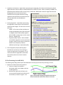
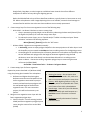
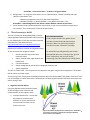
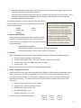
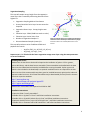
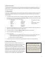
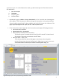
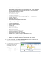
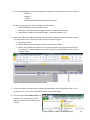
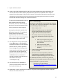
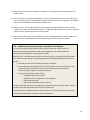
Ecosystem Credit Accounting System
Last updated March 20, 2014. For questions or comments contact us at
[email protected]
Protocol for Quantifying Thermal Benefits of Riparian Shade
Credit Calculation using Shade-a-lator in HeatSource Version 8.0.5 or 8.0.8
The Shade-a-lator model contained in HeatSource Version 8.0.8 (Shade-a-lator) is an approved metric for
calculating Water Quality: Temperature Credits in the Willamette Partnership’s Ecosystem Credit Accounting
System.
Shade-a-lator was developed by Oregon’s Department of Environmental Quality (DEQ)1 to calculate thermal load
reductions (or shade potential), in kcal/day, from riparian shade restoration projects. The assessment’s spatial
unit is a stream reach whose upstream-downstream boundaries are defined by the user, and whose lateral
boundaries extend outward and perpendicular to the stream to a distance also defined by the user, but typically
not more than 150 feet (the usual size of recommended buffers).
Calculating thermal load reductions requires multiple steps:
I.
Acquisition and pre-processing of data layers representing the elevation, topography and vegetation of
the current (or pre-project2) condition and the future (or post-project) condition.
II. Spatial analysis to generate Shade-a-lator inputs. This requires ArcGIS version 9.x or higher, DEQ’s
TTools add-on and the spatial analyst tool set.
III. Run Shade-a-lator on the baseline and post-action condition. The difference between the two is equal to
the shade potential of the restoration design.
I. Data Acquisition and Pre-Processing
Inputs for Shade-a-lator v8.0.8 are generated from running TTools on data representing elevation and landforms
at and around the project site and the height of vegetation communities, including both the existing vegetation
and the anticipated vegetation communities when the project reaches maturity. These data can be acquired
from various sources and will require some pre-processing before TTools can be used.
A. Data Acquisition
The following data layers should be gathered and imported into ArcGIS
1. Recent orthophoto – An aerial photograph of the site that is geometrically corrected (orthorectified) to the
same scale and projection of the other layers. Using an orthophoto will help you stay oriented and guide
digitization of features. Shade-a-lator is typically meant to be run using baseflow conditions, so an
orthophoto representing the stream in late summer or fall is best.
1
http://www.deq.state.or.us/WQ/TMDLs/tools.htm
For more information on defining pre-project and post project conditions, please see the General Crediting Protocol
version 2.0 available at: http://willamettepartnership.org/
2
1
2. Landforms and elevation – Spatial data representing the topography of the bare earth (frequently called a
digital elevation model or DEM). A standard DEM can be used with TTools. Where available, the DEM from
LIDAR data (also called bare earth or last return) is preferred. LIDAR (which stands for Light Detection And
Ranging) data is more accurate and more
DATA SOURCES
convenient for this purpose because existing
Aerial imagery including orthophotos, DEMS and other
vegetation data (#3 below) can be derived from
mapping data can be obtained from:
the same data with minimal additional
- USGS: http://earthexplorer.usgs.gov/
processing.
3. Existing Vegetation - Spatial data representing
the vegetation communities at the site before
restoration work begins. This can come in one of
two forms:
 LIDAR – A first return surface includes tree
canopy and buildings and is often referred to
as a digital surface model (DSM), together
with the DEM, a canopy layer can be created
(Section I. Step B2); OR
 Vegetation Map or photo – Where LIDAR is
not available, vegetation can be represented
through a map of current plant communities
based on the orthophoto, however
additional processing is required (Step B2).
4. Future Vegetation (Project planting plan) –
Describes the area that you are planning to
restore through riparian revegetation. This is
used to forecast the vegetation communities
that will be present when the site reaches
maturity.
LiDAR data is relatively easy to obtain and is sometimes
free. Refer to the following websites to search for
relevant data sets:
-
-
-
USGS LiDAR for various areas in the U.S.
http://earthexplorer.usgs.gov/
Open Topography - limited areas in Oregon
http://opentopo.sdsc.edu/gridsphere/gridsphere?ci
d=datasets
NOAA’s Digital Coast Viewer for DEMs (including
LiDAR), imagery, landcover and socioeconomic data
http://www.csc.noaa.gov/dataviewer/
Map (2008) of LiDAR data availability across Oregon
http://www.blm.gov/or/gis/files/LiDAR_map_11210
8.pdf
If you download an LAS-based LiDAR file, follow the
steps below to create first return and bare earth raster
files:
1. Create an LAS dataset with statistics
2. Filter ground returns in the LAS dataset layer
properties and use the “LAS Dataset to Raster”
to create a bare earth (DEM) raster.
3. Re-filter for non-ground returns in the LAS
dataset layer properties and use the “LAS
Dataset to Raster” to create a first return raster.
B. Pre-Processing (for ArcGIS 10.X)
The following steps will get data layers described above into the proper format for processing in TTools.
1. Digitize river banks and stream centerline
a. Create an empty line shapefile in
ArcCatalog, load it into ArcMap, and start
an editing session.
b. Delineate the right bank, left bank, and
stream centerline based on the direction of
stream flow, as shown in Figure 1. Use
Figure 1: Channel Width Sampling from Digitized Channel Edges at
Each Stream Data Node. Nodes will be created in TTools Step 1
2
Google Earth, Bing Maps, or other images as available to better view the shore from different
viewpoints for better accuracy during the digitizing process.
Banks should be defined as they will be at base flow conditions, typically shown in late summer or early
fall. Where orthophotos or other images depicting this are not available, contact the land manager or
someone familiar with the site to be sure those conditions are accurately represented.
2.
Create canopy layer for the current vegetation in one of the following ways:
 With LIDAR – Use Raster Calculator to create a canopy layer
 A layer representing canopy height can be derived by subtracting the bare earth (Raster2) from
the highest hit (Raster1) to create the canopy raster layer.
 To subtract the raster layers, turn on “Spatial Analyst” Toolbar in ArcMap and open “Raster
Calculator” and enter the following equation:
Minus ([Raster1], [Raster2]) and hit the “Ok” button

Without LIDAR – Digitize current vegetation manually
 In ArcCatalog, create an empty polygon shapefile in the same projection as all other layers. Load
the shapefile you just created into ArcMap and start an editing session for the digitizing process.
 Create polygons for each distinct plant community based on the orthophoto and familiarity with
the site. Attribute each polygon with the height of dominant vegetation using the field
calculator or enter the value directly into the attribute table while in an editing session.
 Vector to Raster – Convert the existing vegetation polygon layer to raster using the same
cell size as the DEM (LIDAR).
ArcToolbox > Conversion Tools > To Raster > Polygon to Raster
3. Create canopy layer for future vegetation
Repeat the process described in 2 (Without LIDAR)
using the planting plan instead of the orthophoto.
a. Delineate and digitize the planting plan.
Delineate areas that are anticipated to have
similar vegetation communities at project
maturity and attribute those polygons with
the anticipated height of the dominant
vegetative strata. For most restoration
projects, this will be the overstory tree
species.
4. Merge current vegetation raster layer with the
future vegetation polygon layer.
a. Vector to Raster – Convert existing (without
LIDAR) and future vegetation polygon layer to
raster using the same cell size as the DEM
(LIDAR)
TIPS - FORMATTING and DATA STORAGE




Naming Convention – Be consistent when
naming files. For files used in GIS, make sure
there are no spaces and keep the name short.
Format - When digitizing features in GIS, use
Shapefiles, which are compatible with TTools,
not a Feature Class within a Geodatabase.
Data Storage - House all of your GIS datasets,
HeatSource model, and model outputs on a
local drive versus a file server or network
drive.
Projection generally a derivation of Lambert
Conformal Conic
3
ArcToolbox > Conversion Tools > To Raster > Polygon to Raster
b. Merge Layers – To merge the raster layers, turn on “Spatial Analyst” Toolbar in ArcMap and open
“Mosaic to New Raster” tool
a. Add current vegetation layer first, then future vegetation.
b. Number of Bands = 1, Mosaic Operator = Last, Mosaic Color Map = First
ArcToolbox > Data Management Tools >Raster > Raster Dataset > Mosaic to New Taster
c. Ensure that the values (associated with the vertical units) in your current and future canopy layers
are in meters. This is necessary for TTools in the next section.
II. TTools Processing in ArcGIS
This tool, an extension developed by DEQ, is used to
sample geospatial data and assemble inputs necessary
for the Shade-a-lator. If you have not done so already,
download the TTools extension here:
http://www.deq.state.or.us/wq/tmdls/tools.htm.
SYSTEM REQUIREMENTS
TTools requires ArcGIS 9.X or greater (but is
unstable in ArcGIS 10.X) and spatial analyst
extension. Make sure you have turned this
extension on under ‘Customize’ in ArcMap.
Based on the landform, elevation and vegetation data,
TTools will create five categories of data:
i.
ii.
iii.
iv.
v.
For ArcGIS 10.X you will generally have to enter
Stream centerline layer and stream
Microsoft VB upon error, reset the script, go to to
centerline nodes;
Tools > References, then turn off missing
Aspect, channel width, right distance and
referencing, then close VB and retry running Ttools.
left distance;
Calculate elevation ;
Sample topography by searching for topographic features; and
Sample Vegetation
You will run TTools twice – first using the current vegetation and again using the future vegetation. The outputs
will be used to run Shade-a-lator.
To start using TTools, simply open the ArcMap document within the downloaded TTools folder. Select the TTools
icon in the toolbar to initiate each of the 5 steps below. The following procedure will follow the exact steps seen
when running TTools.
1. Segment/ Calculate Aspect
Using the digitized stream centerline feature,
TTools will segment the centerline and
calculate aspect at each segment node.
a. Load the centerline file – ensure that
the projection and the stream
direction are correct and that the
stream centerline arrow is at the
mouth of the river.
Figure 2: Illustration showing how the stream aspect is calculated at
each node in TTools (step 1). Illustration from Oregon DEQ Heat
Source Version 7 User’s Manual.
4
b. Define the node distance (25 meters). This process will create a centerline point layer, which is a point
shapefile with points separated by this distance.
Name the output shapefile making sure there are no spaces in the file name (centerline_nodes). If the
last node is unevenly spaced compared to the rest, delete the last node. The rest of the steps will
populate the attribute of this feature.
The attribute table of the newly created point layer will contain a
number of fields. The only ones that should be populated after
Step 1 are the following:
- LENGTH
- STREAM_KM
- LONGDD
2. Measure Channel Widths
-
LATDD
ASPECT
Using the Stream centerline point layer (centerline_nodes),
right bank, and left bank polyline, Step 2 will measure the
channel widths at each segment node. This step will populate
the following fields:
TIPS – CHECK YOURSELF
Each step of TTools should populate new
fields in the attribute table of the
centerline point layer. After each step,
it’s a good idea to open the table to be
sure the right fields are being populated.
If fields are not being populated,
consider checking that you have the
correct system requirements and that
input files are in the proper format.
- CHAN_WID (channel width)
- RIGHTDIST (right distance) - distance from centerline to right bank
- LEFTDIST (left distance) - distance from centerline to left bank
3. Elevation
Use the following inputs to determine stream elevation and gradient based on the DEM (bare earth).




Elevation Correction Method - 9 Cell Sample
Stream Centerline Point Layer - Select the “centerline_nodes” point shapefile
Elevation Layer - Select the DEM raster layer (bare earth)
Elevation Units - Feet
Step three will populate the ELEVATION and GRADIENT attribute fields.
4. Sample Topographic Point Layer
Using the centerline point layer and the elevation layers (DEM), this step samples the topographic shade
angle in either 3 or 7 directions (user-defined) from each stream centerline node. Sampling is done in
the cardinal directions N/E/W. It is okay if Step 4 produces a pop-up that says “Scanned off the grid X
times during processing.” This means that some of the sample points were beyond the extent of the
raster layer.




Stream Centerline Point Layer: select shapefile
Elevation Layer: Select the DEM (bare earth)
Elevation Layer Vertical Units: Feet
Max Sample Distance: 5 km

Number of Directions: 3 (E, S, W)
The following fields should be populated:
TOPO_W
T_LAT_W
T_LON_W
TOPO_S
T_LAT_S
T_LON_S
TOPO_E
T_LAT_E
T_LON_E
5
Vegetation Sampling
This step will sample canopy height from the vegetation
raster layer that is created by subtracting bare earth from
highest hit.







Vegetation Sampling Method: Star Pattern
Stream Centerline Point Layer: Stream centerline
shapefile
Vegetation Raster Layer: Canopy height raster
layer
Elevation Layer : DEM (LIDAR bare earth or other)
Elevation Layer Vertical Units: Feet
Number of Vegetation Samples: 9
Distance between Samples (meters): 8
This step will produce a series of additional fields and
populate the records.
-
Figure 3: Example of land cover sampling performed by
TTools and used as model input in Heat Source (Step5).
Illustration taken from v7.0 DEQ Heat Source user’s
manual.
Veg Elev (ELEV_V1_NE, ELEV_V2_NE, ect)
Veg (Veg1_SE, Veg1_S, ect.)
Repeat steps 1-5 in TTools with the future vegetation canopy raster layer using the same parameters
as current conditions.
Installing Heat Source
Shade-a-lator in Heat Source Version 8.0.8 requires the installation of python 2.5.2 or greater,
python Win32com, and the Heat Source executable. These executables are bundled with the Heat
Source version 8 download and must be installed before running the model. Python pysco 1.63
(which is also included in the download) is an optional installation and is not required to run Heat
Source version 8. We recommend that python pysco be installed because it optimizes the code and
improves model run times. All of these executables may be downloaded (for free) from the internet
from their respective websites.
http://www.python.org
https://sourceforge.net/projects/pywin32/
http://psyco.sourceforge.net/
Shade-a-lator version 8.0.8 also requires Excel 2002 or 2007
Installation instructions:
1. Open the folder “install_executables”.
2. Double click on “python-2.5.2.msi” and follow installation instructions.
3. Double click on “pywin32-210.win32-py2.5.exe” and follow installation instructions.
4. Optional: Double click on “psyco-1.6.win32-py25.exe “ and follow installation instructions.
5. Double click on “heatsource-8.0.0-RC1.win32.exe” and follow installation instructions.
6
III. Run Shade-a-lator
TTools outputs are exported from ArcGIS and moved into the Heat Source spreadsheet in order to run
Shade-a-lator. To run the Heat Source model in Excel, the installation instructions must be followed in
the order listed above.
A. Pre-Processing
After Steps 1-5 TTools have been run for both the current and future vegetation conditions, ensure that
you have all the necessary fields and columns populated and export the tables for use in the Shade-alator calculator.
1. There will be many more fields than you need for the Shade-a-lator calculator, it is helpful to make
the fields you will not need invisible. Go to Properties > Fields in the newly created centerline node
layer and uncheck all but the following fields:
- STREAM KM
- ASPECT
- All Veg (Veg1_SE, Veg1_S,
- LONGDD
- CHAN_WID
ect.)
- LATDD
- RIGHTDIST
- Veg Elev (ELEV_V1_NE,
- TOPO_W
- LEFTDIST
ELEV_V2_NE, ect
- TOPO_S
- ELEVATION
- TOPO_E
- GRADIENT
2. Open the attribute table and check to make sure the fields you checked are visible. This will be the
data that is exported when converting the table to Excel.
3. To export the table to a .dbf, go to Options > Export and name the output table.
4. Open the .dbf tables in Excel and save as .xls
5. Clean-up Excel data
a. Reverse the sorting order (STREAM_KM) of the records so it starts upstream and the last
record is downstream (largest to smallest). This can be done with Custom Sort.
b. Reduce number of significant digits to 3.
6. Create new directories on local drive (i.e. desktop folder) for Heat Source output data files:
B. Shade-a-lator Processing
Familiarize yourself with the model by viewing all the
worksheets. Because only the Shade-a-lator portion of the
Heat Source model will be run, there are only inputs
required for the first four worksheets. Some of the input
data does not impact Shade-a-lator outputs, but is required
by the model code in order to run properly. These fields are
marked with a star (*) in Step B2 below, default values are
provided. The other worksheets contain standardized data
necessary to run the Shade-a-lator model and do not
DON’T SEE THE HEAT SOURCE ADD-IN?
If you do not see the Add-Ins tab, right
click somewhere in the toolbar and select
“Customize Quick Access Toolbar” > AddIns and hit the “Go” button at the bottom
of the page. A pop-up dialogue box will
appear, hit “Ok” and close/restart Excel.
7
require user inputs. To run the Shade-a-lator model, you will need to input the TTools data into these
four worksheets:
i.
ii.
iii.
iv.
Heat Source Inputs
TTools Data
Morphology Data
Continuous Data
1. Reset Model by going to Add-Ins > Setup > Reset Model. Hit “Yes” to confirm that all existing data
will be deleted. If you do not see the Add-Ins tab, right click somewhere in the toolbar and select
“Customize Quick Access Toolbar” and go to Add-Ins and hit the “Go” button and the bottom of the
page. A pop-up dialogue box will appear, hit “Ok” and close/restart Excel.
2. Fill out “Heat Source Inputs” (Figure 3) in the first worksheet tab using the following parameters:
 Simulation Name: Site Name
 Stream length (km) – Denman: 80
 Output path: (C:\models\heatsource\output\)
The directory where the model and output text files will be stored. This should match
the location of the newly created output data file folders.
 Data Start Date* – 10/01/YYYY
*This data start date and data end date (g) are most relevant when using other
portions of Heat Source, but must be filled out for Shade-a-lator to run. Be sure to use
start and end dates that encompass the desired modeling date range (e-f)
Figure 4: Example of Heat Source Inputs (Sheet #1) for HeatSource model.
8






















Modeling Start Date: 10/01/YYYY
Must be within data start/end dates; can be same as Data Start Date. October is often used
because it corresponds with the critical period for temperature in many Oregon streams
and the compliance period for their TMDLs.
Modeling End Date: 10/31/YYYY
Data End Date*: 10/31/YYYY
Flush Initial Condition (days)*: 5
Time offset from UTC (hours) – while on Daylight Savings Time: -7; rest of the year: -8
Time Step – dT (min): 1
Distance Step – dX (m): 25
Average Distance for the longitudinal sample rate: 25
Longitudinal Sample Rate (m): 25
Should always be 1: 1 with Distance Step
Transverse Sample Rate (m): 8
Number of transverse samples: 9
Inflow Site*: 0
Continuous Data Site*: 1
Wind function* coefficient a
Wind function* coefficient b
Include Deep Alluvium Temperature*: FALSE
Deep Alluvium Temperature*: Leave blank
Account for Emergent Veg Shading*: Leave blank
LIDAR data used for veg codes: True (False if LiDAR data was not used)
Landcover density for LIDAR data: 0.75
Landcover stream overhang for LIDAR data (m): 0
Vegetation angle calculation method: point (if using LiDAR data, zone, otherwise)
3. In the Heat Source toolbar, select ‘Setup’ > Setup Data Sheets (Figure 5). This will set up the data
sheets to be populated based on the Heat Source inputs.
4. In the “TTools Data” worksheet (tab #2)
cut and paste columns into the
corresponding portions of the
worksheet.
- LONGDD - TOPO_E
- LATDD
- Veg0_EMERG
- TOPO_W - All Veg
- TOPO_S - All ELEV
Figure 5: Heat Source Toolbar - Setup Data Sheets
9
5. In the “Morphology Data” worksheet (tab #4) cut and paste TTools data into the first four columns.
- Distance
- Elevation
- Gradient
- Bottom Width (Channel Width from TTools data)
Use the following inputs for the other fields on this worksheet
 Channel Angle: 0 (constant simplified value)
 Mannings n: 1 (refers to surface roughness, does not affect the calculation)
 Parameters for sediment and heat exchange* (use default values for all)
6. Data in the “Continuous Data” worksheet is not required for Shade-a-later, but Heat Source needs
at least one value in the “continuous node” column, as shown in Figure 4.
 Continuous node: 1
 Node: Indicate a position along the stream centerline (e.g. middle)
 Stream (km): Indicate the distance from the stream segment origin where this position lies.
For example, in a stream segment that is 0.8km long, if you select “Middle,” enter 0.4 in the
Stream km field.
Figure 4: Continuous Data worksheet for Heat Source model
7. Errors are relatively common when first setting up Heat Source and running Shade-a-lator. If you
encounter errors, refer to the Troubleshooting tips and resources below.
8. Run the model: Run > Shade-a-lator only
(Figure 6). This will produce a .txt file
within the output folder created on the
desktop.
Figure 6: Heat Source Toolbar – Run Shade-a-lator Only
10
9. Import .txt file into Excel
10. Create a new Excel workbook with four tabs. The first tab provides basic project information. The
next two tabs will be used to hold the output data from the two runs of Shade-a-lator. Output is
reported as hourly averages of solar flux to the stream. The last tab will be used to create the credit
calculation by converting this into kilocalories per day and comparing the two scenarios to get the
thermal load reduction resulting from restoration activities.
The entire Excel workbook will be shared
with Willamette Partnership during
Verification, name each worksheet in a
way that is clear and consistent with file
naming conventions used throughout.
An example workbook is available from
Willamette Partnership. The workbook
contains example formulas and
supplementary instructions for the final
steps of converting and comparing Shadea-lator outputs to get project uplift.
11. Cut and paste the contents of the Heat
Source SR4 output .txt file (Step 8) for
the baseline condition into the second or
Baseline tab. Each column represents
hourly averages of solar loading on the
stream at each node. Create a new row
just below the one that indicates the
position (in km) of each node. Use the
AVERAGE function to calculate the
average the values of each column and
store then in this row (ex.
=AVERAGE(D5:D748)).
12. Use instructions in the workbook to
paste and transpose these values into
the Credit Calculation tab.
Tips – Troubleshooting
HeatSource can be difficult to run and you may encounter
errors when you run the final calculations. IF this happens,
try the following troubleshooting tips.
1. Save, re-open, re-run
2. Make sure all python scripts are downloaded
correctly (downloaded in the proper order,
program file saved in the proper location)
3. If the output values seem incorrect (Step 12,
above), work backwards to find the origin of the
error.
 Make sure all columns are pasted
correctly from TTools (.dbf), or .txt
files, into Excel.
 Make sure all arrays match
 Did you fill in all the data sheets
properly?
4. Ensure that no other Excel files are open when
you run the model.
5. Set Excel to run in XP compatibility mode and
rerun Heatsource. Heatsource may generate a
readable message identifying your source of error.
For additional information on the stream processes,
digitizing in GIS, and model operations refer to the User’s
Manual published for a previous version.
-
Heat Source v7.0 Users Manuel:
http://www.deq.state.or.us/wq/tmdls/docs/tools
/heatsourcemanual.pdf
13. Repeat Steps 1-10 to run Heat Source model for the future riparian vegetation conditions and paste
data into the third or Future tab.
11
14. Repeat Step 12 for the future condition, making sure to arrange the data consistently with the
baseline data.
15. Use instructions in the example workbook to import the wetted width for each node and convert
Solar Flux (W/m2) to Solar Load (Kilocalories/Day). Conversion factors are supplied in the example
workbook and embedded in the example workbook cells.
16. Create a column in the Credit Calculation tab to subtract average loading values for the future
condition from those of the baseline condition. The difference between the two values is the shade
potential of the restored riparian forest at each node.
17. Sum all these values to get the total difference in solar loading between the baseline and future
conditions. This is shade potential of the proposed riparian forest restoration actions.
TIPS – SUBMITTING CREDIT CALCUALTIONS TO WILLAMETTE PARTNERSHIP
For users that are generating shade for water quality temperature credits under the
Willamette Partnership Ecosystem Credit Accounting System, the credit calculation is
submitted via the Ecosystem Crediting Platform (ECP).
When the user is satisfied that the model was run correctly on scenarios that match intended
or as-built restoration designs. The following materials should be uploaded to the project on
the ECP:
 HeatSource workbooks for baseline and future conditions
 Excel workbook containing data from the SR4 for baseline and future conditions, and
comparison of the scenarios for a final value of shade potential converted to
Kilocalories/day (as shown in example workbook).
 Data layers and features used in TTools
o LIDAR bare earth or other DEM
o LIDAR first return or digitized current vegetation
o Digitized planting plan
o Digitized stream banks, stream centerline
The ECP can handle large file sizes, but please contact Willamette Partnership if you encounter
trouble loading files and need to transmit files in another way.
To facilitate timely review of submitted materials, please use consistent conventions to name
files and clearly label tabs or columns in the Excel workbook.
12