Download fulltext - DiVA Portal

Master's Degree Thesis
ISRN: BTH-AMT-EX--2005/D-15--SE
Analysis of Compliance Maps
with MATLAB Toolbox
Gorrepati Haribabu
Chinthalapalle Chandrasekhar Reddy
Department of Mechanical Engineering
Blekinge Institute of Technology
Karlskrona, Sweden
2005
Supervisor:
Kjell Ahlin, Professor Mech. Eng.
Analysis of Compliance Maps
with MATLAB Toolbox
Gorrepati Haribabu
Chinthalapalle Chandrasekhar Reddy
Department of Mechanical Engineering
Blekinge Institute of Technology
Karlskrona, Sweden
2005
Thesis submitted for completion of Master of Science in Mechanical
Engineering with emphasis on Structural Mechanics at the Department of
Mechanical Engineering, Blekinge Institute of Technology, Karlskrona,
Sweden.
Abstract:
Structural dynamics engineers are asked to make measurements for
distinguishing differences between two structures. A frequent approach
is to compare the modal parameters by change in Modal Assurance
Criterion behaviour which focuses only on the Eigen values and Eigen
vectors.
A Graphical method of comparison was found for simple structures,
which considers the spatial distribution of the entire frequency response
spectrum. Point compliances represented by a color scale are measured
at short intervals along reference line on a structural edge and the result
is a three dimensional representation of dynamic behaviour. Experiments
were conducted and MATLAB toolbox along with Graphical User
Interface for compliance maps was built.
Keywords:
Experimental Modal Analysis, Frequency Response Functions,
Compliance Maps, Dynamic Frequency Mobilyzer, accelerometer,
MATLAB.
Acknowledgements
This thesis work was carried out at the Department of Mechanical
Engineering, Blekinge Institute of Technology, Karlskrona, Sweden, under
the guidance of Prof. Kjell Ahlin.
In particular we wish to express our sincere appreciation to our supervisor
Prof. Kjell Ahlin for his engagement and professional guidance throughout
the work. Also his contribution during the long days when the
measurements were performed is highly acknowledged.
All this work would not be possible without the generous donation of ski
“XRC 500 RAILFLEX II” for experimentation by Mr. Anders Holmdin,
Interski AB. We express our sincere appreciation to “HEAD®” for not only
providing the required ski but also to produce quality ‘TPS’ systems.
Finally, we would like to thank our parents and friends for their extended
support indirectly during the thesis work.
Karlskrona, April 2005.
Haribabu Gorrepati.
Chinthalapalle Chandrasekhar Reddy.
2
Contents
1 Notation
5
2 Introduction
7
3 Theory of Modal Analysis
3.1 Multiple Degrees of Freedom System
3.2 Frequency Response Measurements
3.2.1 Types of FRFs
3.2.2 The FRF Matrix Model
3.3 Modal Testing
3.3.1 Measuring FRF Matrix Rows or Columns
3.3.2 Exciting Modes with Impact Testing
3.4 Data Acquisition
3.5 Modal Parameter Extraction
3.6 Definitions of Waterfall Diagrams and compliance maps
3.6.1 Waterfall diagrams
3.6.2 Compliance maps
3.6.3 Waterfall diagrams Vs Compliance maps
9
10
13
14
15
15
16
17
18
18
20
20
20
20
4 Experimentation
4.1 Simulated Rectangular plate
4.2 Rectangular plate
4.4 Measurement preparations
4.4.1 Suspension of the structure
4.4.2 Selection of excitation points
4.4.3 Method to excite the structure
4.4.4 Method to excite the structure
4.4.5 Accelerometer considerations
4.4.5.1Type of accelerometer
4.4.5.2Mounting techniques
4.4.5.3Accelerometer calibration
4.5 Experimental setup
4.6 Analysis
22
22
22
25
25
26
27
28
29
29
30
30
31
32
5 Results and Discussion
5.1 Results of Simulated rectangular plate
5.2 Results of rectangular plate
5.3 Results of Skis
33
33
37
40
3
6 Conclusion and Recommendations
44
7 References
45
A User’s Manual
1 Introduction
2 Window layouts of the GUI
3 Start and run the program at the first time
4 List of MATLAB® functions supplied by Saven Edutech®
46
46
47
49
50
4
1 Notation
A(ω )
Accelerance (m/sec 2 )
c
Damping (N sec/m)
[C]
Damping matrix (Ns/m)
f
Force (N)
F
Frequency (Hz)
{F}
Force vector or input signal (N)
[H]
Transfer function matrix (rad/sec)
[H ( ω )]
Frequency response function (-)*
k
Spring coefficient (N/m)
[K]
Stiffness Matrix (N/m)
m
Mass (kg)
[M]
Mass matrix (kg)
N
Number of mode of interest (DL)*
s
Laplace operator (DL)*
t
Time variable (sec)
x
Displacement (m)
{x}
Time varying displacement vector
{X}
Response vector or out put signal (-)*
x&
First derivative with respect to time of dependent variable x
&x&
Second derivative with respect to time of dependent variable
{x&}
Time varying velocity vector
{ &x& }
Time varying acceleration vector
V (ω )
Mobility (m/sec)
ω
Angular frequency
5
Indices
0
Initial conditions
i
ith Degree of freedom
j
jth Degree of freedom
k
kth Degree of freedom
x
X-direction
y
Y-direction
z
Z-direction
Abbreviations
SDOF
Single Degree of Freedom
MDOF
Multi Degree of Freedom
FFT
Fast Fourier Transform
EMA
Experimental Modal Analysis
DFM
Dynamic Frequency Mobilyzer
UFF
Universal File Format
TPS
Traction Power System
6
2 Introduction
Vibrations are inherent to life though generally mankind regards them as
unpleasant causing undesirable consequences as discomfort, noise,
malfunctioning, wear, fatigue and even destruction.
Therefore strong and reliable vibration analysis tools are a basic need of
modern engineering. Modal analysis is one of those tools. There are many
methods to distinguish differences between two structures within modal
analysis, but the draw back with all these methods is that these cannot give
you the visualization of the above said differences.
Background
A collection of a series of high quality, closely spaced FRFs over some
length or area can be used to visualize and show for efficiently comparing
the dynamic properties of structures. This visualization is termed
Compliance Maps [1]. Work has been carried out in this field by Gary C.
Foss [1], where Compliance maps were drawn for trusses, Snowboards,
Wing Spar mill fixtures etc.
Aim and Objective
This thesis is an attempt to extend work on this new visualization tool to
mark the differences between two structures. Compliance maps were drawn
for various skis. A MATLAB program with a graphical user interface was
designed for plotting compliance maps.
The main objectives of the thesis can be listed as
•
•
•
•
Study of various methods for comparison of Structures
Simulation of rectangular plate in MATLAB followed by
Experimentation on same in the Laboratory, for acquaintance in
Modal parameter extraction, Water fall diagrams and compliance
maps.
Extension of the experimentation on Skis of different ages and
plotting the compliance maps.
Development of a MATLAB toolbox along with a GUI to enable
plotting of compliance maps for any given data.
7
This report explains the various theories behind Modal parameter
extraction, Water fall diagrams and compliance maps followed the
description of experimental setup in chapter 4. Results of the experiments
are presented in chapter 5 followed by conclusions. The toolbox and GUI
are explained in Appendix A.
8
3 Theory of Modal Analysis
Modal analysis is primarily a tool for deriving reliable models to represent
the dynamics of structures. Modal analysis aims to develop reliable
dynamic models that may be used with confidence in further analysis. In
general, it can be said that the applications of modal analysis today cover a
broad range of objectives like,
•
•
•
•
•
•
Identification and evaluation of vibration phenomena
Development of experimentally based dynamic models
Structural integrity assessment
Structural modification and damage detection
Model integration with other areas of dynamics such as acoustics,
fatigue, etc.
Establishment of criteria and specifications for design, test,
qualification and certification
Models of vibrational mechanical systems consider mainly masses,
stiffness and damping. Every model uses assumptions for simplification
and therefore contains uncertainties from the outset. Because of the
increasing importance of a preferable precise estimation of the model
parameters, the computer aided measurement and analysis of dynamical
properties of components play a more and more decisive role. A structure’s
actual dynamical behaviour can merely be investigated experimentally. The
Experimental Modal Analysis (EMA) is one of the most important
measurement procedures in this area.
The EMA uses transfer functions of a system, i.e. the relationship between
‘system input’ (driving forces) and ‘measured system response signals’
(accelerations at one or more points on the structure). The measured time
domain signals are transformed into the frequency domain. Each transfer
function gained from a single output-input combination is one component
of the overall system. From this the modal quantities Eigen frequencies,
damping parameters and eigenvectors (spatial displacements at the points
of measurement at the respective Eigen frequency also called mode shapes)
can be calculated. The knowledge of the modal quantities allows a
9
description of the dynamic behavior and is the basis of further numerical
investigations.
Modes (or resonances) are inherent properties of a structure. Resonances
are determined by the material properties (mass, stiffness, and damping
properties), and boundary conditions of the structure. Each mode is defined
by a natural (modal or resonant) frequency, modal damping, and a mode
shape. If either the material properties or the boundary conditions of a
structure change, its modes will change. At or near the natural frequency of
a mode, the overall vibration shape (operating deflection shape) of a
structure will tend to be dominated by the mode shape of the resonance [2].
3.1 Multiple Degrees of Freedom System
The degrees of freedom of a system are the number of independent
coordinates necessary to completely describe the motion of that system.
The simplest possible discretisation of a system, denoted as a SDOF (Single
Degree of Freedom), was introduced as a model capable of describing its
dynamic behaviour in the simplest possible terms. The advantage of this
initial approach is that it makes it a lot easier to understand most of the
basic concepts and their physical meaning. However, most real mechanical
systems and structures cannot be modelled successfully by assuming a
single degree-of-freedom, i.e. single coordinate to describe their vibratory
motion.
Real structures are continuous and non homogeneous elastic systems which
have an infinite number of degrees of freedom. Therefore their analysis
always entails an approximation which consists of describing their
behaviour through the use of a finite number of degrees of freedom, as
many as necessary to ensure enough accuracy.
10
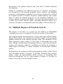
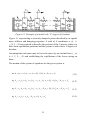
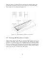
Figure 3.1. Example of a model with ‘N’ degrees of freedom.
Figure 3.1 representing a viscously damped system described by its spatial
mass, stiffness and damping properties. A total of N coordinates x i (t) ( i
=1,2,3…,N) are required to describe the position of the N masses relative to
their static equilibrium positions and the system is said to have N degrees of
freedom.
Assuming that each mass may be forced to move by an external force f i (t)
(i=1, 2, 3…, N) and establishing the equilibrium of the forces acting on
them.
The motion of the system of equations for the given system is,
m1.&x&1 + (c1 + c2 ).x&1 − c2 .x&2 + (k1 + k 2 ).x1 − k 2 .x2 = f1
(3.1)
m2 .&x&2 − c2 .x&1 + (c2 + c3 ).x& 2 − c3 .x&3 − k 2 .x1 + (k 2 + k3 ) x2 − k3 . x3 = f 2
(3.2)
m3 .&x&3 − c3 .x&2 + (c3 + c4 ).x&3 − c4 . x&4 − k3 . x2 + (k3 + k 4 ).x3 − k 4 .x4 = f 3
(3.3)
m4 .&x&4 − c4 .x&3 + c4 .x&4 − k 4 .x3 + k 4 .x4 = f 4
(3.4)
11
.
m N .&x&N − c N .x& N −1 + (c N + c N +1 ).x& N − k N .x N −1 + (k N + k N +1 ).x N = f N (3.5)
A convenient method to solve the above system of equations is to use
matrices.
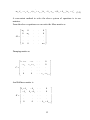
From the above equations we can write the Mass matrix as
 m1
 0

M = .

 .
 0
0
.
.
m2
.
.
.
.
.
.
.
.
0
.
.
0 
0 
. 

. 
m N 
Damping matrix as
c1 + c 2
 −c
2

C= .

 .
 0
− c2
. .
c 2 + c3
. .
.
. .
.
. .
0
. .


0


.

.

c N + c N +1 
0
And Stiffness matrix is
k1 + k 2
 −k
2

K = .

 .
 0
− k2
. .
k 2 + k3
. .
.
. .
.
. .
0
. .


0


.

.

k N + k N +1 
0
12
For a multiple degrees of freedom system, the system of equations can be
written as in the form of matrix notations is,
[M ]{&x&} + [C ]{x&} + [K ]{x} = { f }
(3.6)
Where [M], [C], and [K] are Mass, Damping and Stiffness symmetric matrices,
&&} , {x&} and
these matrices describes the spatial properties of the system. {x
{x} vectors are time varying acceleration, velocity and displacement
responses, and {F} is the time varying external excitation forces.
By taking Laplace transform on both sides of the above equation we will
get,
L([M ]{&x&} + [C ]{x&} + [K ]{x}) = L({ f })
(3.7)
( Ms 2 + Cs + k ).X ( s ) = F
(3.8)
Equations (3.1) to (3.5) are second order, linear and time invariant
differential equations. Since the system is coupled it must be solved
simultaneously. By assuming that the system is un-damped the solution is
obtained. Since the system is coupled it has to be manipulated to form an
Eigen value problem. The resulting Eigen value represents the frequencies
of the modes and the eigenvectors are the mode shapes.
3.2 Frequency Response Measurements
The frequency Response Function (FRF) is a fundamental measurement
that isolates the inherent dynamic properties of a mechanical structure.
Experimental Modal Parameters (Frequency, damping and mode shape) are
also obtained from a set of FRF measurements.
The FRF describes the input-output relationship between two points on a
structure as a function of frequency. Since both force and motion are vector
quantities, they have directions associated with them. Therefore, an FRF is
13
actually defined between a single input DOF (point & direction), and a
single output DOF.
Frequency Response Function is a measure of how much displacement,
velocity or acceleration response a structure has at an output DOF per unit
of excitation force at an input DOF as a function of frequency.
FRF is the ratio of the Fourier transform of an out put response X ( ω ) to
the Fourier transform of input force F ( ω ).
Figure 3.2. Definition of FRF.
3.2.1 Types of FRFs
Motion can also be expressed as acceleration or velocity. For modal
analysis, the most common form of the FRF is the normalized acceleration
response or accelerance.
A(ω ) =
A
F
(3.9)
The inverse of accelerance is called the apparent mass. The velocity FRF is
called the mobility.
V (ω ) =
V
F
(3.10)
14
The inverse of mobility is called the mechanical impedance. The
displacement response function H (ω ) is called the dynamic compliance or
receptance and the inverse of this is called the dynamic stiffness.
H (ω ) =
X
F
(3.11)
The choice of displacement, velocity or acceleration depends on the
phenomena of interest. If amplitude and frequency are logarithmically
scaled, the choice will affect the average slope of the FRF and hence
scaling relative to frequency. Since the measurements are typically made
with an accelerometer, accelerance and apparent mass are the easiest
quantities to display. However, displacement, stiffness and compliance are
more useful and intuitive quantities for comparing structures whose
performance depends on resistance to displacement.
3.2.2 The FRF Matrix Model
A structural dynamics measurement involves measuring elements of an
FRF matrix model for the structure. This model represents the dynamics of
the structure between all pairs of input and output DOF's. The FRF matrix
model is a frequency domain representation of a structure’s linear
dynamics, where linear spectra (FFT’s) of multiple inputs are multiplied by
elements of the FRF matrix to yield linear spectra of multiple outputs.
FRF matrix columns correspond to inputs and rows correspond to outputs.
Each input and output corresponds to a measurement DOF of the test
structure. The FRF measurements on a structure are shown in figure 3.3.
3.3 Modal Testing
In modal testing, FRF measurements are usually made under controlled
conditions, where the test structure is artificially excited by using either an
impact hammer, or one or more shakers driven by broadband signals. A
multi-channel FFT analyzer is then used to make FRF measurements
between input and output DOF pairs on the test structure. Here for the SKI
structure we used impact hammer method.
15
When the output is fixed and FRFs are measured for multiple inputs, this
corresponds to measuring elements from a single row of the FRF matrix.
This is typical of a roving hammer impact test.
Figure 3.3. Measurements of FRFs on a structure.
3.3.1 Measuring FRF Matrix Rows or Columns
Modal testing requires that FRFs be measured from at least one row or
column of the FRF matrix. Modal frequency and damping are global
properties of a structure, and can be estimated from any or all of the FRFs
in a row or column of the FRF matrix. On the other hand, each mode shape
is obtained by assembling together FRF numerator terms (called residues)
from at least one row or column of the FRF matrix.
16
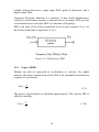
3.3.2 Exciting Modes with Impact Testing
Impact testing is the most popular modal testing method used today. It is a
fast, convenient and low cost way of finding modes of the structure. The
test equipment to perform the operation is an impact hammer with a load
cell attached to its head to measure the input force, an accelerometer to
measure the response acceleration at a fixed point and direction, a two or
four channel FFT analyzer to compute FRFs.
An example of time signal of input and response and their spectrums are
shown in the Figure 3.4a and Figure 3.4b respectively.
Figure 3.4(a). Impulse and Response signals (Time Domain).
Figure 3.4(b). Impulse and Response Spectrums.
17
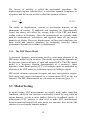
3.4 Data Acquisition
The used data acquisition system is of type SignalCalc Mobilyzer®
manufactured by Data Physics ® Corporation. The setup of the Mobilyzer®
is shown in Figure 3.5
Figure 3.5. SignalCalc Mobilyzer® Setup.
3.5 Modal Parameter Extraction
One of the most fundamental assumptions of modal testing is that a mode
of vibration can be excited at any point on the structure, except at nodes of
vibration where it has no motion. Hence, a single row or column of the
18
frequency response matrix provides sufficient information to estimate
modal parameters. As a result, the frequency and damping of any mode in a
structure are constants that can be estimated from any one of the
measurements as shown in Figure 3.6, In other words, the frequency and
damping of any mode are global properties of the structure.
In practical applications, it is important to include sufficient points in the
test to completely describe all the modes of interest [11]. If the excitation
point has not been chosen carefully or if enough response points are not
measured, then a particular mode may not be adequately represented. At
times it may become necessary to include more than one excitation location
in order to adequately describe all of the modes of interest. Frequency
responses can be measured independently with single-point excitation or
simultaneously with multiple-point excitations. The mode shapes as a
whole are also global properties of the structure, but have relative values
depending on the point of excitation and scaling and sorting factors. On the
other hand, each individual modal coefficient that makes up the mode shape
is a local property in the sense that it is estimated from the particular
measurement associated with that point as shown in figure 3.6.
Damping frequency – Same at each Measurement Point
Mode Shape – Obtained at same frequency from all measurement points
Figure 3.6. Concepts of modal parameters.
19
3.6 Definitions of Waterfall Diagrams and
compliance maps
3.6.1 Waterfall diagrams
Waterfall diagram is a 3-dimensional representation with frequency on the
x-axis amplitude on the y-axis and nodes of the structure on the z-axis.
Figure3.7 shows a mobility waterfall diagram created on a simulated
rectangular plate in MATLAB®.
3.6.2 Compliance maps
Compliance maps are color diagrams with frequency on the x-axis physical
position on y-axis and color scale represents amplitude.
The FRF magnitudes should usually be scaled logarithmically. This
displays the FRF peaks and dips with equal symmetry. For compliance
color-maps, this means opposite colours equally represent extremes of
stiffness or compliance and deep blue would represent large apparent mass
[1].
Viewing data in this way gives a depiction of how the dynamic properties
distribute themselves both spectrally and spatially. The peaks of
accelerance line up at constant frequency and vary only in amplitude,
defining the mode shape along the reference line. For drive point FRFs,
every resonance is followed by anti resonance. The anti-resonance do not
line up at a single frequency. Their frequencies wander with position from
the node line at one mode to node line at next mode.
3.6.3 Waterfall diagrams Vs Compliance maps
As an alternative to the waterfall diagram, the data can be displayed as a
color map shown in the figure3.7 .The color scale now represents amplitude
and the Y direction represents physical position. This type of threedimensional display improves on the waterfall diagram for conceptualizing
the spatial as well as spectral nature of structural dynamic behaviour. The
modes show up as vertical bars of high accelerance (yellow and or red).The
anti-resonance areas are distinguished as dark blue or green valleys of high
20
apparent mass. These features are not distorted, as they are in the waterfall
display. As used here, the term anti-resonance refers to a local minimum in
an FRF.A node would be a location where anti-resonance intersects with a
mode frequency, indicating no motion at that location for the mode.
Figure 3.7. Water fall Diagram vs. Compliance Maps.
21
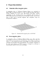
4 Experimentation
4.1 Simulated Rectangular plate
A rectangular plate of 2000mm × 1000mm × 100mm was simulated in
MATLAB® as shown in figure 4.1 with 12 nodes on each side with a
Young’s Modulus of 2.1*1011 N/m2, and density 7850 kg/m3. Various
experiments on the simulated plate were conducted with the help of
MATLAB® functions provided by Saven Edutech® and the results in the
form of FRF curves, waterfall diagrams and compliance maps are
incorporated in chapter 5.
Figure 4.1. Simulated Rectangular plate in MATLAB.
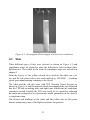
4.2 Rectangular plate
A rectangular plate of 990mm × 128mm × 30mm was taken and the
experiments were performed by attaching mass tuned damper as shown in
Figure 4.2. The construction of mass tuned damper was made with the help
of sponge and Swedish coins glued together. The resonance frequency of
the mass tuned damper an SDOF system is changed by reducing or
increasing the number of the coins accordingly.
22
Figure 4.2. Rectangular Plate hanged with free-free conditions.
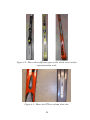
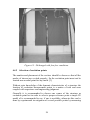
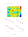
4.3 Skis
Three different types of skis were selected as shown in Figure 4.3 and
compliance maps are plotted to show the differences between these three
different skis. The results in the form of compliance maps are included in
chapter 5.
From the Figure 4.3 the yellow colored ski is obsolete, the white one is in
use and the red colored ski is new and supplied by ‘HEAD®’ – a leading
sports gear manufacturing company in the world.
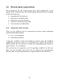
The white and the red skis came with TPS (Traction Power System) as
shown in Figure 4.4 and the manuals which accompanied the skis indicated
that the TPS aids in making wide and tight turns in different ski conditions
extremely smooth. Initially the TPS was tested for its operations although
the main aim remained as to represent the modal parameters in the form of
a compliance map.
The fixtures and bindings on the white and the yellow skis act like point
masses attenuating some of the higher resonance frequencies.
23
Figure 4.3. Shows three different types of skis which were used for
experimentation work.
Figure 4.4. Shows the TPS on red and white skis.
24
4.4 Measurement preparations
The preparations for the measurements have great significance to the
quality of the collected data. The measurements should be done according
to the following steps.
•
•
•
•
•
Suspension of the structure
Selection of excitation point
Method to excite the structure
Selection of measurement points
Accelerometer considerations
4.4.1 Suspension of the structure
There are two different ways to suspend the structure when performing
experimental modal analysis.
•
•
Free –free conditions
Operating conditions
A free-free condition is the best method to measure since the boundary
conditions are easy to achieve in a repeatable way. In this the energy is
mainly spread into the structure not into the surrounding parts.Figure4.5
shows the free –free conditions.
The second way of suspension is in its operating conditions in this case
there are two possible ways. This can be achieved by experimenting
directly while in operating conditions or approximated in the laboratory.
25
Figure 4.5. Ski hanged with free-free conditions.
4.4.2 Selection of excitation points
The number and placement of the exciters should be chosen so that all the
modes of interest are excited properly. So the excitation point must not be
located near a nodal point for any mode [3].
Without prior knowledge of the dynamic characteristics of a structure the
location of excitation measurement points is a matter of trial and error
coupled with experience and engineering judgment.
Generally it is recommended to choose one corner of the structure as
excitation point but in order to select a proper reference point a simple FE
model of is recommended to use, if one is available, otherwise this can be
done by experimental investigation of several possible points by measuring
26
the driving point frequency response. This can be done with the use of a
single accelerometer and a roving impact hammer.
4.4.3 Method to excite the structure
The excitation mechanism is constituted by a system which provides the
input motion to the structure under analysis. There are two types of
excitation methods possible for measurement of FRFs for modal analysis of
a structure.
•
•
Impact hammer excitation
Shaker excitation
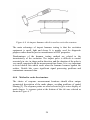
Impact hammer excitation is the best choice to excite small structures. An
impact hammer is simply a hammer with various attachable masses and tips
which serve to extend the frequency and force ranges of the impact as
shown in figure 4.6. An integral part of the hammer is a force transducer,
which uses the compression of a piezoelectric crystal to detect the
magnitude of the force felt by the hammer when it strikes a structure. The
magnitude of the force is determined by the mass of the hammer head and
the velocity with which it is moving when it hits the structure. When
operated by hand, it is usually easier to vary the velocity, so the force level
may be adjusted by changing the mass of the hammer head. The frequency
range of excitation provided by a hammer is determined by the stiffness of
the hammer-structure contact surfaces and the mass of the hammer head.
27
Figure 4.6. An impact hammer which is used to excite the structure.
The main advantage of impact hammer testing is that the excitation
equipment is small, light and cheap. It is mainly used for diagnostic
purposes rather than for precise measurement of FRF properties.
Disadvantages of the hammer testing method are related to the
inconsistency of the excitation. The impact pulse is difficult to control
accurately in size, in shape and in direction, and the duration of the pulse is
very small compared with the measurement time frame. It is very important
to avoid double hits which result when the hammer bounces against the
surface. Double hits cause significant signal processing problems and
contaminate measured data.
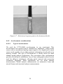
4.4.4 Method to excite the structure
The choice of response measurement locations should allow unique
geometrical description of the mode shapes, avoiding problems of spatial
aliasing [2]. The response points are often selected to give a nice display of
mode shapes. A response point at the bottom of the ski was selected as
shown in Figure 4.7.
28
Figure 4.7. Selection of response point at the bottom of the ski.
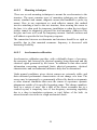
4.4.5 Accelerometer considerations
4.4.5.1
Type of accelerometer
We used the 8772A5M10 accelerometer in our experiment. This
accelerometer can operate both as standard low impedance, voltage mode
sensor with a conventional analog output signal or in a digital piezo smart
sensor mode capable of providing pertinent information stored with in its
memory module. This type of accelerometer is ideally suited for multi
channel modal analysis applications. The convenient cubic configuration
provides flexibility for installation. Any of three orthogonal surfaces can be
used for adhesive attachment, allowing quick removal and convenient
orientation alignment. Main applications are for multi channel
measurements, Modal analysis measurements on automotive body and
aircraft frames and structural analysis measurements.
29
4.4.5.2
Mounting techniques
There are several mounting techniques to mount the accelerometer to the
structure. The most common types of mounting techniques are adhesive
mount, standard stud mount, magnetic mount and handheld or probe tip
mount. Here in our experiment we used adhesive mount, this method
involves attaching a base to the test structure, then securing the sensor to
the base, it is often used for temporary installation or when the test object
surface cannot be adequately prepared for stud mounting. Adhesives like
hot glue and wax well work for temporary mounts. Smooth surfaces and
stiff adhesives provide the best frequency response.
The connection between accelerometer and structure should be as rigid as
possible, due to that mounted resonance frequency is decreased with
increasing flexibility.
4.4.5.3
Accelerometer calibration
Accelerometer calibration provides, with a definable degree of accuracy,
the necessary link between the physical quantity being measured and the
electrical signal generated by the sensor. In addition to that other useful
information concerning operational limits, physical parameters, electrical
characteristics and environmental influences may also be determined.
Under normal conditions, piezo electric sensors are extremely stable, and
their calibrated performance characteristics do not change over time. The
sensor may be temporarily or permanently affected by harsh environments
or other unusual conditions that cause the sensor to experience dynamic
phenomena outside of its specified operating range. This change manifests
itself in a variety of ways, like a shift of the sensor resonance due to a
cracked crystal, a temporary loss of low-frequency measuring capability
due to a drop in insulation resistance or total failure of the built –in
microelectronic circuit due to a high mechanical shock.
30
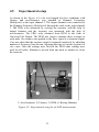
4.5
Experimental setup
As shown in the Figure 4.8 a ski was hanged free-free conditions with
fixtures and accelerometer was attached to Dynamic Frequency
Mobilyzer® at the input channel 2. The impact hammer was connected to
the Dynamic Frequency Mobilyzer® through the cable at the input channel
1. The FRFs were measured by exciting the structure with the help of
impact hammer and the response was measured with the help of
accelerometer. The FRFs were obtained from DFM in the form of
Universal File Format. The DFM was setup to measure three averages at
each node. No window was applied as the force signal is a transient signal.
Care was taken that the response signal is captured completely by adjusting
number of frequency lines in turn, adjusting the time to capture response or
vice versa. Once the settings were fixed in the DFM same settings were
used for all nodes. Hammer is moved from one node to another to excite
the structure.
1) Accelerometer, 2) Fixtures, 3) DFM, 4) Roving Hammer
Figure 4.8. Experimental setup for ski FRF measurement.
31
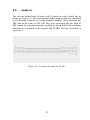
4.6
Analysis
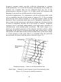
The ski was divided into 48 nodes with 16 nodes on each vertical line as
shown in Figure 4.9. The experimental modal analysis data was measured
at 48 different locations by roving hammer method. After obtaining the
FRF data in the form of UFF files they were converted into the form of
FRF matrix by using the functions supplied by Saven EduTech® and these
functions are explained in the chapter MATLAB® tool box described in
Appendix A.
Figure 4.9. Location of nodes on the Ski.
32
5
Results and Discussion
5.1 Results of Simulated rectangular plate
Firstly, a rectangular plate was simulated and various experiments were
conducted using MATLAB®. Plotting frequency response functions before
and after attaching mass tuned damper were some of the cases dealt with.
The FRFs are expressed in the form of Waterfall diagrams and the same
plots are shown in the form of Compliance maps. We have conducted
experiments on the rectangular plate in laboratory and compared the results
from simulation. This followed experiments on skis and Compliance maps
were drawn. In the last phase we made a MATLAB tool box for the
analysis of compliance maps along with graphical user interface (GUI).
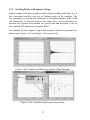
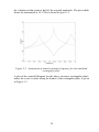
Figure 5.1 shows the FRF of the simulated rectangular plate.
Fi
gure 5.1. FRF of the simulated rectangular plate.
The resonance frequency at 18.17 Hz has the maximum amplitude. Now
with the help of a mass tuned damper we aimed at 18.17 Hz and attenuated
33
the vibration at that point to half of the original amplitude. The plot which
shows the attenuation at 18.17 Hz is shown in figure 5.2.
Figure 5.2. Attenuation of aimed resonance frequency for the simulated
rectangular plate.
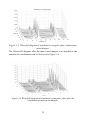
A plot of the waterfall diagram for the above structure (rectangular plate),
where the z-axis is nodes along the border of the rectangular plate, is given
in Figure 5.3.
34
Figure 5.3. Waterfall diagram of simulated rectangular plate without mass
tuned damper.
The Water fall diagram after the mass tuned damper was attached to the
structure in consideration can be observed in Figure 5.4.
Figure 5.4 Waterfall diagram of simulated rectangular plate after the
attachment of mass tuned damper.
35
The respective compliance maps without damping and with damping are
shown in Figures 5.5 and Figure 5.6 respectively.
Figure 5.5. Compliance map of simulated rectangular plate without mass
tuned damper.
A clear red vertical stripe is observed at about 18.7 Hz as depicted by
Figure 5.5. This stripe is observed to be split into two vertical stripes
(Figure 5.6) with a decrease in the color intensity indicating amplitude
attenuation which is achieved by the attachment of mass tuned damper.
Anti-resonance occurs at the tuned frequency and the vibration is decreased
by a large fraction.
36
Figure 5.6. Compliance map of simulated rectangular plate after the
attachment of mass tuned damper.
5.2
Results of rectangular plate
A rectangular plate of 990mm × 128mm × 30mm was taken and the
experiments are performed by attaching mass tuned damper. The
Compliance map plotted before attaching the mass tuned damper is shown
in Figure 5.7.
37
Figure 5.7. Compliance map of rectangular plate before the attachment of
mass tuned damper.
Four resonance frequencies at 17, 46, 76 and 92 Hz are observed in Figure
4.7and in these resonances mass tuned damper was aimed at 92 Hz. The
construction of mass tuned damper was made with the help of sponge and
Swedish coins glued together. The resonance frequency of the mass tuned
damper which is nothing but an sdof system is changed by reducing or
increasing the weight of the coins accordingly. In this way the mass tuned
damper was tuned to 92 Hz and the compliance map plotted is shown in
Figure 5.8.
38
Figure 5.8. Compliance map of simulated rectangular plate after the
attachment of mass tuned damper.
It can be observed from the figure that the 92 Hz resonance frequency was
attenuated to a large extent. The inaccuracy in the construction of the mass
tuned damper led to damping of the unaimed resonance at 76 Hz.
39
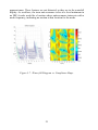
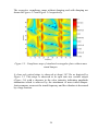
5.3 Results of Skis
The Compliance map of the yellow ski is shown in the Figure 5.9
Figure 5.9. Compliance map of the yellow ski and four mode shapes.
40
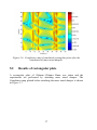
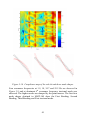
Figure 5.10. Compliance map of the red ski and three mode shapes.
Four resonance frequencies at 1.9, 18, 34.7 and 59.5 Hz are observed in
Figure 5.9 and at dominant 4th resonance frequency torsional mode was
observed. The higher modes are damped by the point masses. The first four
mode shapes obtained in MATLAB show the First Bending, Second
Bending, Third Bending and First torsional mode.
41
Figure 5.10 shows the compliance map for the red ski, as observed the
torsional mode at the 3rd resonance frequency is damped due to the TPS.
The first four resonance frequencies are at 19.6, 39.9, 68.1 and 143.9 Hz.
The first three mode shapes obtained in MATLAB show the First Bending,
Second Bending and First torsional mode.
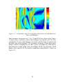
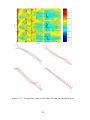
Figure 5.11 shows the compliance map for the white ski, as observed the
torsional mode at the 4th resonance frequency is damped due to the TPS.
The first four resonance frequencies are at 2.0, 6.4, 32.5 and 52.6 Hz. The
four mode shapes obtained in MATLAB show the First Bending, Second
Bending, Third Bending and First torsional mode. There was a good
agreement in the scaling of the yellow and red skis but a scaling change is
observed in this case. However, the scaling does not affect the working of
the TPS. It was observed that the compliance map was inaccurate when
ever it was tried to modify to fit along the scale of yellow and red skis.
42
Figure 5.11. Compliance map of the white ski and four mode shapes.
43
6 Conclusion and Recommendations
Structural dynamics engineers are frequently asked to make measurements
for the purpose of distinguishing differences between two structures or
changes within the same structure. A frequent approach is to compare the
modal parameters by following a shift in modal frequency or a change in
modal assurance criterion between two sets of Eigen vectors. But the
weakness of this approach is that it ignores the total dynamic behaviour and
focuses only on the Eigen values and Eigen vectors.
This thesis is an Extension work of the new visualization tool to mark the
differences between two structures. Compliance maps were drawn for
various skis. A MATLAB program with a graphical user interface was
designed for plotting compliance maps.
A visualization tool has been shown for efficiently comparing the dynamic
properties of structures. This technique requires the collection of a series of
high quality, closely spaced FRFs over some length or area. It permits
quick graphical comparisons, allows the identification of mode shapes for
simple structures, and offers additional insight on the spatial and spectral
distribution of modal parameters and general dynamic behaviour.
Future work could take into consideration the following points
•
•
•
•
More experiments on different simple structures are required.
IDEAS model could be built and validated with the help of
experimental data presented in this work.
The MATLAB® tool box can be extended by including more
number of functions and look and field of the GUI could be
improved by adding more choices for the end user.
Further work is required on the scaling of amplitude in the form of
color intensity in plotting compliance maps.
Work can be done in studying the comparisons between
Compliance maps and other tools of Visualization.
44
7 References
1
Gary C. Foss., (2004), Compliance Maps: A Graphical Tool for
Making Structural Comparisons, Structural Dynamics Lab, Boeing
Commercial Airplane Group, Seattle.
2
Shahram Ajdari and Nicklas Claesson.,(2004), Modal Analysis of a
Carbon Fibre Surface Vessel, Masters Thesis, Department of
Mechanical Engineering, Blekinge Institute of Technology, Karlskrona,
Sweden.
3
Ahlin k. and Brandt A.,(2001), Experimental Modal Analysis in
Practice, Saven EduTech AB, Taby, Sweden.
4
Anders Brandt.,(2001), Introductory Noise & Vibration Analysis,
Saven Edutech AB and The department of Telecommunications and
Signal Processing, Blekinge Institute of Technology, Sweden.
5
Nuno M. M. Maia and Julio M. M. Silva., (1997), Theoretical and
Experimental Modal Analysis, Instituto Superior Tecnico, Portugal.
6
Dr. Randall J. Allemang, Vibrations: Analytical and Experimental
Modal Analysis, Structural Dynamics Research Laboratory,
Department of Mechanical, Industrial and Nuclear Engineering,
University of Cincinnati.
7
D. J. Ewins, (2000), Modal Testing: Theory, Practice and Application,
2nd edition, Research studies press.
8
K. G. McConnell, (1995), Vibration Testing: Theory and Practice,
Wiley.
9
W. G. Halvorsen and D. L. Brown, (1977), Impulse Technique for
Structural Frequency Response Testing, Sound & vibration.
10 Patrick Marchand and O. Thomas Holland, Graphics and GUIs with
MATLAB, 3rd edition, NVIDIA, The Naval Surface Warfare Center
Dahlgren Division.
11 The Fundamentals of Modal Testing, Application Note 243-3, Agilent
Technologies, U.S.A.
45
A User’s Manual
1
Introduction
The program is useful to plot compliance maps from universal files
obtained by doing experiments on the structures with the help of
experimental setup explained in chapter4.5. Therefore the knowledge about
experimental modal analysis is required and UFF files must be ready to use
in this tool box.
A MATLAB® function called ‘uicontrol’ is introduced to create the
graphic objects in this program, which are user interface controls and they
activate call back routines when users activate the objects. There are
number of user interface controls like push button, radio button, editable
text and menus.
The graphical interface part of the program that is used here was created by
use of functions from Saven EduTech®. The functions activate uicontrol
objects.
After the user had read this manual he will have a good understanding of
this MATLAB® program and also will be able to use the program.
46
2
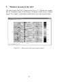
Window layouts of the GUI
The start screen of the GUI is shown in the Figure 2.1. It shows an example
plot of Compliance map. In the bottom left corner of the screen a button
tagged ‘Give Inputs’ is provided to enable user to give the required inputs.
Figure 2.1. Start screen with ‘give inputs’ button.
47
Figure 2.2. User input data window.
As soon as the user hits the ‘Give inputs’ button in the start screen, a new
window pops up titled ‘Give Inputs’. It contains 3 edit boxes, 5 static texts
3 mutually exclusive radio buttons and 1 push button. In Figure 2.2 the
number of UFF files which are used by the user to plot the compliance
maps can be entered, the default value in the edit box ‘1000’ (Represented
by 1). Frequency range of interest can be entered in 2 and 3. The default
value for minimum frequency is ‘0’ and the default value for maximum is
‘78’. User can select the type of UFF files from ‘Dynamic Flexibility’,
‘Mobility’ and ‘Accelerance’ (represented by 4). User can plot the
compliance map after the inputs are entered in the respective edit boxes and
hitting the ‘Plot’ button (represented by 5).
48
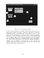
Figure 2.3. Result window with compliance map.
After, the user hits the ‘plot’ button in the second screen the Compliance
map is plotted with in the frequency range of interest entered as input. The
compliance map is shown in the Figure 2.3.
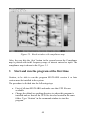
3
Start and run the program at the first time
Caution, to be able to run the program MATLAB® version 6 or later
version must be installed in the system.
The procedure is divided into the following steps
•
•
First of all start MATLAB® and make sure that UFF files are
available.
Change the default or working directory to where this program is
installed and see that all the UFF files are also located in the same
folder. Type ‘Guistart’ in the command window to start the
program.
49
•
•
4
The first window contains a button at the bottom left corner push
the button to enter the inputs.
After entering the inputs in the second screen and hitting the “plot”
button the result plotting compliance map opens in a separate
window.
List of MATLAB® functions supplied by Saven
Edutech®
anybutt.m
uitext.m
radiobut.m
editbox.m
fullscrn.m
animate.m
animate2.m
geodef.m
modeplot.m
cvfrfa2v.m
cvfrfd2v.m
univread.m
uf2frf.m
animate.m
animate2.m
animcalc.m
complexp.m
htoeplitz.m
poleadd.m
impresp.
50
Department of Mechanical Engineering, Master’s Degree Programme
Blekinge Institute of Technology, Campus Gräsvik
SE-371 79 Karlskrona, SWEDEN
Telephone:
Fax:
E-mail:
+46 455-38 55 10
+46 455-38 55 07
[email protected]