Download KINSIM User`s Manual. Bruce A. Barshop Washington University

KINSIM User’s Manual.
Bruce A. Barshop
Washington University
Biological Chemistry
Computing Facility
30 December 1983
CHAPTER 1
OVERVIEW OF THE SIMULATION SYSTEM.
CHAPTER 2
THE SIMUL COMMAND PROCEDURE.
CHAPTER 3
COMPILING A KINETIC MECHANISM.
3.1
INTRODUCTION. . . . . . . . . . . . . . . . . . . 3-1
3.2
THE TEXTUAL MECHANISM DESCRIPTOR FILE. . . . . . . 3-1
3.2.1 Chemical Equations. . . . . . . . . . . . . . . 3-2
3.2.2 Output Equations. . . . . . . . . . . . . . . . 3-3
3.3
EXAMPLE TEXTUAL MECHANISM FILES. . . . . . . . . . 3-4
3.3.1 Uni-Uni Enzyme Reaction . . . . . . . . . . . . 3-4
3.3.2 Bi-Bi Enzyme Reactions . . . . . . . . . . . . . 3-5
3.3.3 Feedback activation . . . . . . . . . . . . . . 3-6
3.3.4 Feedback inhibition . . . . . . . . . . . . . . 3-7
3.4
SUMMARY TABLE OF MECHANISM SYMBOLS. . . . . . . . 3-8
3.5
KINETIC COMPILER ERROR CODES. . . . . . . . . . . 3-9
CHAPTER 4
PERFORMING A KINETIC SIMULATION
4.1
LOADING A MECHANISM. . . . . . . . . . . . . . . . 4-1
4.2
SETTING PARAMETERS. . . . . . . . . . . . . . . . 4-2
4.2.1 In-house Version: . . . . . . . . . . . . . . . 4-2
4.2.2 Portable Version: . . . . . . . . . . . . . . . 4-3
4.2.3 Setting Time Parameters. . . . . . . . . . . . . 4-3
4.3
SAVING AND RESTORING PARAMETERS. . . . . . . . . . 4-5
4.4
INCLUDING DATA. . . . . . . . . . . . . . . . . . 4-5
4.4.1 Real Data And Simulated Data. . . . . . . . . . 4-7
4.5
FITTING INCLUDED DATA. . . . . . . . . . . . . . . 4-7
4.6
KINSIM OUTPUT OPTIONS. . . . . . . . . . . . . . . 4-7
4.6.1 Display. . . . . . . . . . . . . . . . . . . . . 4-7
4.6.2 List. . . . . . . . . . . . . . . . . . . . . . 4-8
4.6.3 Plot. . . . . . . . . . . . . . . . . . . . . . 4-8
4.6.4 Output. . . . . . . . . . . . . . . . . . . . . 4-8
4.7
INTERRUPTIONS OF SIMULATION. . . . . . . . . . . . 4-8
4.7.1 Elective Abortion. . . . . . . . . . . . . . . . 4-8
4.7.2 Simulation Errors. . . . . . . . . . . . . . . . 4-8
4.8
RUN TIME ERRORS. . . . . . . . . . . . . . . . . . 4-9
4.8.1 Initialization Errors. . . . . . . . . . . . . . 4-9
4.8.2 Fatal Errors. . . . . . . . . . . . . . . . . . 4-9
4.8.2.1
Mass Conservation Errors. . . . . . . . . . . 4-9
4.8.2.2
Integration Errors. . . . . . . . . . . . . . 4-9
4.8.2.3
Floating Overflow And Divide-by-zero Errors. . 4-9
4.8.2.4
Excessive Computation. . . . . . . . . . . . 4-10
4.8.3 Catastrophic Errors. . . . . . . . . . . . . . 4-10
APPENDIX A
ABBREVIATIONS AND SPECIAL SYMBOLS USED.
Page 2
APPENDIX B
CONVENTIONS FOR SPECIFICATION OF FILES.
APPENDIX C
AFTER THE SIMULATION SESSION.
APPENDIX D
DATA FILE STRUCTURE.
D.1 THE DATA FILE HEADER STRUCTURE. . . . . . . . . . D-2
D.2 THE DATA STRUCTURE. . . . . . . . . . . . . . . . D-3
D.3 CONVERTING DATA. . . . . . . . . . . . . . . . . . D-3
APPENDIX E
IMPLEMENTATION NOTES.
E.1
MODULE NOTES. . . . . . . . . . . . . . . . . . . E-1
E.2
INCLUDEd files and PARAMETERs. . . . . . . . . . . E-2
E.3
STORAGE REQUIREMENTS OF KINSIM. . . . . . . . . . E-3
E.3.1 Relationship Between KINCOMP And KINSIM. . . . . E-5
E.4
REPRESENTATION OF CHARACTER DATA. . . . . . . . . E-5
E.5
HEADER NOTES. EXTRACTING AND SUPPRESSING SECTIONS
OF CODE. . . . . . . . . . . . . . . . . . . . . . E-6
E.6
PROGRAM FLOW AND OVERLAYING. . . . . . . . . . . . E-8
E.7
GRAPHICS ROUTINES NOT PROVIDED. . . . . . . . . . E-8
E.8
INSTALLATION SUMMARY. . . . . . . . . . . . . . E-10
APPENDIX F
SAMPLE SIMULATIONS
APPENDIX G
MAINTENANCE.
APPENDIX H
HEADER NOTES.
Index
CHAPTER 1
OVERVIEW OF THE SIMULATION SYSTEM.
Version 3.3
19 May 1983
<CR><LF>
NOT the lastest version but sufficient ---May,1990
The programs described constitute a flexible and powerful system
for the simulation of full time course reactions. In general there are
three steps to simulating a given mechanism and each step is carried out
by a separate program.
1.
Mechanism entry: A chemical reaction scheme is typed, using
conventional chemical format. The text editor of the user’s
choice is used to generate the textual mechanism descriptor
file.
2.
Compilation: The kinetic compiler is run which reads the
textual mechanism file and assembles tables of information
about the reaction scheme and the symbols used, which are
written in a binary mechanism descriptor file.
3.
Simulation: The simulator is a general program which can in
principle depict any chemical mechanism at all. It reads the
binary mechanism descriptor file output by the compiler to
provide it with the necessary information to carry out the
simulation of the given mechanism.
This manual describes the operation of the kinetic compiler and the
simulator.
The programs described in this manual have been developed on a
Digital Equipment Corporation VAX 11/780 computer at the Washington
University Medical School- Biological Chemistry Computer Facility
(WUMS-BCCF). Chapters 3 and 4 are the important user-oriented sections.
Certain sections of this document are intended only to be of interest to
local users at the WUMS-BCCF. The sections of local interest only are:
Chapter 2, Appendices B, C and D. Appendix E is a semi-technical
section with suggestions for the installation and implementation of the
system.
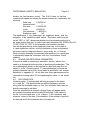
CHAPTER 2
THE SIMUL COMMAND PROCEDURE.
At the WUMS-BCCF (*), the programs are integrated through the use
of a single command procedure. It is necessary to have two logical
names in the process table:
($) Assign User$Disk:[CFlab.Simul] Sim:
($) Assign User$Disk:[CFlab.Stopflow] Sf:
To invoke the command procedure, then type:
($) @Sim:Simul .
A parameter to the command procedure is used to determine which type of
graphics terminal is being used. That parameter can be passed directly:
($) @Sim:Simul VT125, or
($) @Sim:Simul VT640,
or the procedure will prompt the user when necessary. If the terminal
type is passed directly, then further parameters can be used, to be
quickly executed as commands. For example:
($) Simul :== @Sim:Simul VT125
($) Simul Compile Test.Mec
($) Simul Help Data Converting, etc., etc.
Extensive help is available on-line through this command procedure. The
help facility makes use of the best features of the VAX/VMS HELP
utility, and all users are urged to make use of it.
The option menu for the command procedure is:
--------------------(*) Refer to appendix A for abbreviations used.
THE SIMUL COMMAND PROCEDURE. Page 2-2
Commands are:
Edit
: edit a kinetic mechanism.
Compile
: compile an existing mechanism.
Simulate
: perform a simulation.
Display
: display stopped-flow/simul files.
Merge
: merge stopped-flow/simul files.
Debug
: debug a compiled mechanism.
DCL
: execute a one-line DCL command.
Spawn
: enter a subprocess.
Reattach
: exit the subprocess.
Exit
: leave the room.
For additional help, type HELP [ topic ].
The options “EDIT”, “COMPILE”, and “SIMULATE” correspond to the three
essential steps of the simulation process. A simplified outline for
executing the SIMUL command procedure is included below.
1.
If the mechanism to be simulated has already been successfully
compiled, proceed to step 3. If a new mechanism is to be
generated or an existing mechanism is to be changed, choose
“Edit”. The EDT editor will be invoked. Refer to Chapter 3
for format of mechanism descriptor file.
2.
Choose “Compile” to compile the specified mechanism. If an
error ensues, you may return to step 1.
3.
To carry out a simulation, choose “Simulate”. Refer to Chapter
4 for details of simulation.
(A)
Load a mechanism, by typing “M<CR>.”
(B)
Set initial concentrations of reactants, by typing “C<CR>”.
Return to option menu by typing “<ESC>”.
(C)
Set values of the factors to be used in output of
simulation, by typing “F<CR>”. Return to option menu by
typing “<ESC>”.
(D)
Set rate and/or dissociation constants, by typing “K<CR>”
(Concentrations and kinetic constants must be in the same
units). Return to option menu by typing “<ESC>”.
(E)
Set timing and coordinate scaling parameters, by typing
“T<CR>”.
a)
Set the run time and ymax.
b)
As a first approximation, use an integration/point
value of one and a delta time of 0.001 times the run
time.
(i)
If no equilibrium steps are included in the
mechanism, as a first approximation, set Flux
tolerance = 0.1 and Integral tolerance = 0.001
(ii)
If equilibrium steps are in the mechanism, as a
first approximation, set Flux tolerance = 0.1 and
Equilibrium rapid = YES
THE SIMUL COMMAND PROCEDURE. Page 2-3
If real data is included, the procedure is the same
except that the run time and ymax are set
automatically.
(F)
Carry out the simulation, by typing “G<CR>”.
(G)
To terminate the simulation session, type “Q<CR>”. You
will be returned to the level of the SIMUL command
procedure.
4.
To exit the SIMUL command procedure, choose “Exit”.
Note that there are many other functionalities in the SIMUL command
procedure, including data file display and manipulation. Refer to the
on-line help.
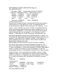
CHAPTER 3
COMPILING A KINETIC MECHANISM.
3.1
INTRODUCTION.
The kinetic compiler, KINCOMP, is the program which renders a
human-readable representation of a kinetic mechanism into an internal
form. Its input is a text file (the textual mechanism descriptor file),
written according to the conventions outlined below. The text file is
parsed by the compiler, and a binary file (the binary mechanism
descriptor file) is created, which is used as a “load module” to provide
the run-time program, KINSIM, with the information required to simulate
a specific mechanism. The text file can easily be created with the use
of any editor. When the compiler is run, it will prompt for the name of
an input textual mechanism descriptor file. The file name is specified
as outlined in appendix B. The file will be read and the mechanism will
be kinetically parsed. If no errors are detected, a prompt will be
issued for the output file name for the output binary mechanism
descriptor file.
3.2
THE TEXTUAL MECHANISM DESCRIPTOR FILE.
The textual mechanism descriptor file consists of two major
sections: the first section contains the chemical equations and the
second contains the output equations. The chemical equations define the
reaction scheme and the output equations define the variables to be
graphed during the simulation.
Notes:
Delineation: The two sections of the text file must be
separated with a line containing an asterisk (*) in column
number 1.
Comments: An exclamation point (!) in the text file indicates
that the remainder of that line is a comment to be ignored by
the compiler.
Title: A line which has a dollar sign ($) in column number 1
is used to entitle the mechanism; the text on that line is
included to identify the output of all simulations performed
with that mechanism. Including a title is entirely optional.
COMPILING A KINETIC MECHANISM. Page 3-2
3.2.1 Chemical Equations.
These equations are entered in standard chemical format. Each
species in the mechanism is represented by a unique name of up to ten
characters which may be any combination of letters and numbers.
Monomeric species are represented by single letters and their complexes
are represented as combinations of letters and numbers. Numbers
preceeding a species name signify multipliers and numbers following a
component name signify stoichiometric constants. For example:
“A” represents a monomeric species, and
“AA” or “A2” represents the dimer of that species.
“2A2” represents two dimers of “A”, and
“2AB3O4” represents two molecules, each of 1 A, 3 B’s and 4
O’s.
Chemical steps in the mechanism are represented by equal signs.
Two equal signs in succession (==) signify a step which is rategoverned, that is a step with both a forward and reverse rate constant.
A single equal sign (=) specifies a rapid equilibrium step, which will
be forced to equilibrate at the beginning of each cycle in the
integration of the mechanism. Only one parameter is used to describe an
equilibrium step, and it is always a dissociation constant (regardless
of the direction in which the step is written).
There is a limit of forty chemical steps to a mechanism. The steps
may be entered individually on separate lines or as many as desired may
be entered on a single line, subject to the limitation that only the
first eighty characters of each line of the text are read by the
compiler. If the steps are chemically consecutive, they may be
concatenated:
“ E + S == ES == EP == E + P “.
If non-consecutive steps are entered on one line, they must be separated
with a semicolon:
“ E + S == ES ; E + I == EI “.
Presently, only two types of mass conservation attributes are
implemented for chemical species, of the following types:
Attribute.
Action.
0 (Default) Concentrations are checked to assure that they
never become negative.
1
The attributed species’ concentration is held
constant at the initial level set by the user.
An attribute is assigned to a species by typing a left bracket ([)
followed by the attribute number, immediatedly following a species name.
Any species may have only one attribute. Each species need have its
attribute specified only once, even if the species appears in multiple
steps. For mass conservation attribute one (constant concentration),
the number 1 may be omitted; that is “A[” is interpreted as “A[1”.
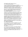
COMPILING A KINETIC MECHANISM. Page 3-3
3.2.2 Output Equations.
The output equations allow the concentration units used for a
simulation to be converted to other units (for example, absorbance) for
direct comparison of simulated data to experimental data. The output
expressions are specified in standard FORTRAN-style algebraic notation,
with the following rules and restrictions:
(1)
Operand parameters are indicated as the species’ names already
used in the mechanism or may be names not previously used.
Species’ names refer to the species concentrations. Names not
present in the reaction scheme are used to define adjustable
output factors to be set by the user at run-time (for example,
extinction coefficients).
(2)
In addition to adjustable output factors which can be set at
run-time, a mechanism may include fixed numerical values in its
output calculations. To include a value, the number is entered
preceeded by a number sign (#). The number may be specified in
integer, floating point, or exponential notation. Thus, the
following are the same: “A*#2”, “A*#2.0”, “A*#2.E0”.
(3)
The mathematical operators are:
1.
2.
3.
4.
5.
6.
(4)
^
*
/
+
%
(up-arrow)
(asterisk)
(slash)
(plus)
(minus)
(percent)
Exponentiation.
Multiplication.
Division.
Addition.
Subtraction.
Logarithm (Naperian).
Mathematical operators have the standard priorities:
% > ^ > *,/ > +,Parentheses can be used to resolve ambiguous expressions. For
example: A+B*C adds A to the product of B and C. and (A+%B)*C
multiplies C by the sum of A and log B.
(5)
Output expressions may consist of more than one line of text,
provided that each unfininshed line ends with an underline
character (). Thus it is possible to specify long
calculations in a single expression. For example, the
predicted saturation of a site obeying the Monod-Wyman-Changeux
equation may be calculated as a function of a changing
concentration of species S in a single output expression:
( S*(#1+S)^(n+#1) + L*c*S*(#1+c*S)^(n+#1) ) /
( (#1+c*S)^n + L*(#1+c*S)^n )
(6)
The value last calculated for an output expression may be used
in another output calculation. In this case, the output
channel number to be referenced is indicated as an integer
preceeded by an at-sign (@). For example, the preceeding
output expression could have been specfied in two output
expressions:
1.
S*(#1+S)^(n+#1) + L*c*S*(#1+c*S)^(n+#1)
2.
@1 / ( (#1+c*S)^n + L*(#1+c*S)^n )
COMPILING A KINETIC MECHANISM. Page 3-4
3.3
EXAMPLE TEXTUAL MECHANISM FILES.
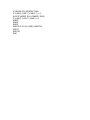
3.3.1 Uni-Uni Enzyme Reaction
The mechanism depicted below represents the simple enzyme reaction
catalyzed by fumarase. In this mechanism, E represents the enzyme, F
its substrate fumarate and M the product malate.
! Fumarase mechanism.
! Comment.
$FUM1
! Mechanism title.
E + F = EF == EM = E + M ! Reactions.
*OUTPUT
! Output expressions follow.
EF*X1 + F*X2 - X3
! Two output
EM*X4 + M*X5 - X6
! ...expressions.
In the mechanism depicted above, the characters to the right of the
exclamation points (!) are comments, ignored by the compiler. Notice
the following features illustrated in the example:
1.
The first and third reactions are treated as rapid equilibria.
Although these two reactions are written from right to left as
association and dissociation steps, the constants associated
with both these equilibria are to be entered as dissociation
constants.
2.
The output expressions include the names of species in the
reaction scheme as well as output constants. The first output
expression will equal the concentration of the enzyme-substrate
complex (EF) times its extinction coefficient (X1) plus the
concentration of the substrate (F) times its extinction
coefficient (X2) minus some offset factor (X3). At run-time
the values of the factors may be set for any particular
display. For example, if the values of X1, X2 and X3 are set
to 0., 1. and 0. respectively, the first output will simply
equal the concentration of F.
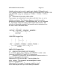
The compiler will assemble a transcription of the mechanism
representation which can be displayed at run-time to refresh the user’s
memory. The reaction steps will be numbered sequentially and the rate
and equilibrium constants will be identified by these numbers. The
transcribed form of this particular mechanism will appear as follows:
FUM1
K1
K+2
K3
E + F = EF ; EF == EM ; EM = E + M
K-2
OUTPUT 1 = EF*X1 + F*X2 - X3
OUTPUT 2 = EM*X4 + M*X5 - X6
COMPILING A KINETIC MECHANISM. Page 3-5
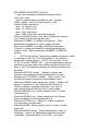
3.3.2 Bi-Bi Enzyme Reactions
The mechanisms below depict two schemes for bi-bi enzyme reactions.
The first one is a compulsory order for substrate addition and the
second one has a random addition. The first, OBIBI, is represented with
all rate-governed steps and is simple to understand. The second,
REBIBI, has rapid equilibrium steps for addition of the substrates and
dissociation of the products. Note that there is only a single
rate-governed step in the REBIBI mechanism. Also note that the steps
EB + A = EAB and EP + Q = EPQ could not be included as equilibrium steps
in REBIBI, to avoid the likelihood of violating the principle of
microscopic reversibility.
$OBIBI - Ordered Bi-Bi
$REBIBI - Random equilibrium Bi-Bi
E + A == EA
E + A = EA ; E + B = EB
EA + B == EAB == EQ + P EA + B = EAB == EPQ
EQ == E + Q
EQ + P = EPQ
E + Q = EQ ; E + P = EP
F1*P
*
F2*Q
F1*P
F3*E
F2*Q
F4*A
F3*E
F5*B
F6*EA+F7*EAB
F8*EQ
COMPILING A KINETIC MECHANISM. Page 3-6
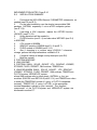
3.3.3 Feedback activation
The mechanism depicted below represents a more complicated scheme
of feed-back activation of an enzyme. It could be considered as a
superficial representation of the phosphofructokinase reaction.
$OSCIL1P1. Oscillating system, N=1, P=1.
!
! Inexhaustible pool, constant infusion.
POOL[1 == A
! Michaelis-Menten reaction.
E + A = EA == E + B
! Non-linear (M-M) drain reaction. Infinite sink.
F + B = FB == F + SINK[1
! Produce activation.
E + B = EB
EB + A = EBA == EB + S
!
Output equations:
!
A*X1
B*X2
(E+EA)*X3
(EB+EBA)*X4
In this mechanism, E represents the regulatory enzyme, A its substrate,
and B its product. The upper glycolyic pathway is represented as a
reaction which results in a constant infusion of substrate. The lower
glycolytic pathway is represented as a non-linear system (i.e., a single
enzyme F) for the removal of product. Notice that the species
represented as “POOL” is given a special mass conservation attribute of
type 1, as it is represented as “POOL[1”. This (if K-1 .EQ. 0 )
assures that the influx of A is at a constant rate. Similarly, the
“SINK” is limitless and, if fixed at zero concentration, even if K-5 is
non-zero, the reaction will not reverse. Although back reaction could
simply be eliminated by making K-5 equal to zero, with time there might
be a danger of numeric overflow in the computer, if the “concentration”
of SINK is not kept at zero.
A noteworthy feature of this system is that it can sustain
oscillations. This is not only an extremely interesting phenomenon to
study, but also a very effective test for each installation of this
simulator. Refer to appendix F for sample parameter values.
COMPILING A KINETIC MECHANISM. Page 3-7
3.3.4 Feedback inhibition
The mechanism depicted below represents a scheme of feed-back
inhibition of an enzyme in a series of reactions.
$OSCIL8P2. Oscillating system, N=8, P=2.
!
POOL[1 == S1
! Constant infusion.
E1 + S1 = E1S1 == E1 + S2 ! A series of ...
E2 + S2 = E2S2 == E2 + S3 ! ...
E3 + S3 = E3S3 == E3 + S4 ! ...
E4 + S4 = E4S4 == E4 + S5 ! Michaelis-Menten...
E5 + S5 = E5S5 == E5 + S6 ! reactions...
E6 + S6 = E6S6 == E6 + S7 ! ...
E7 + S7 = E7S7 == E7 + S8 ! ...
E8 + S8 = E8S8 == E8 + S9 ! ...
E9 + S9 = E9S9 == E9 + SINK[1 ! Removal by final enzyme.
E1 + 2S9 = E1’
! Feedback inhibition.
E1’ + S1 = E1S1’ == E1’ + S2 ! Inhibited reaction.
*OUTPUT
S2*X1
S3*X2
S4*X3
S5*X4
S6*X5
S7*X6
S8*X7
S9*X8
Note that we take advantage of the leniency of the compiler here. Since
the compiler does not enforce mass balance, the numeric suffixes of the
species’ names are not treated as stoichiometries. Refer to appendix F
for sample parameter values.
COMPILING A KINETIC MECHANISM. Page 3-8
3.4
SUMMARY TABLE OF MECHANISM SYMBOLS.
Symbol
Significance
======
============
==
Kinetic reaction step Separates reactants and products.
=
Rapid equilibrium reaction step Separates components and complex.
Co-reactants Separates species participating in a reaction step.
L{x}
Chemical species Names are <= 10 characters, begin with alphabetic.
nL{x}
Reaction stoichiometry Indicates that species reacts with stoichiometry n.
L{x}An{x} Component stoichiometry Indicates component A is present with stoichiometry n.
L{x}{’} Isomer Trailing apostrophe(s) may be used to distinguish species.
L{x}[n
Mass conservation Endows species with mass conservation attribute n.
!
Comment Text after exclamation point (!) is ignored.
$
Mechanism title Text on line with dollar sign in column 1 used as title.
Section delimiter Asterisk (*) in column 1 is used to
separate the chemical and output equations.
%,+,-,*, Mathematical symbols /,^,(,)
Used in the output equations.
Conventions used in this table:
=========== ==== == ==== ======
x indicates any alphanumeric character.
L and A indicate any alphabetic character.
n indicates any numeric character.
{} indicates any number of occurances of enclosed sequence.
COMPILING A KINETIC MECHANISM. Page 3-9
3.5
KINETIC COMPILER ERROR CODES.
The compiler contains a simple error facility. If an error is
encountered in parsing the mechanism, one of the following error
messages will appear and the offending line of text will be displayed
(where applicable).
Module
Error #
REACTION ANALYZER:
21)
Species found where delimiter expected.
22)
Delimiter found where species expected.
23)
Semicolon, but unfinished step.
24)
Unexpected delimiter.
25)
Reaction control block overflow.
26)
Species descriptor block overflow.
SPECIES ANALYZER:
41)
Zero length species name/ adjacent delimiters.
42)
Species with no components/ misplaced leading delimiter.
43)
Multiply specified isomerization/ misplaced apostrophe.
44)
Multiply attributed species.
45)
Invalid attribute value/ unexpected character at end of name.
46)
Component encountered after attribute/isomer specification.
47)
Illegal character in species name/ unindentified error.
EQUATION COMPILER:
61)
Too many output calculation instructions.
62)
Syntax error in species name used in output expression.
63)
Variable name with non-alphabetic first symbol.
64)
Missing operator after closing parenthesis.
65)
Unbalanced parentheses ( “)” without “(“ ).
66)
Unrecognized math operator.
67)
Unbalanced parentheses ( “(“ without “)” ).
68)
Output constant symbol overflow.
69)
Output calculation stack overflow.
70)
No output specified.
71)
Illegal output channel reference.
72)
Output constant overflow.
73)
Decode error in output constant.
74)
Too many output expressions.
EQUILIBRIUM GENERATOR:
81)
Not a binding equilibrium.
82)
Too many complexes.
83)
Recursion in equilibria.
84)
Too many components.
CHAPTER 4
PERFORMING A KINETIC SIMULATION
The initial display in KINSIM is the main menu prompt:
KINSIM
Version 3.3
Chemical Kinetic Simulation System.
Options- V = View mechanism
M = Load mechanism
C = Change concentrations
K = Change rate constants
F = Change output factors
T = Change time factors
ON
D = Toggle display output
OFF
L = Toggle list output
OFF
O = Toggle binary output
OFF
P = Toggle plot output
OFF
I = Toggle inclusion of real data
OFF
A = Toggle agreement to real data
S = Save parameters
R = Restore parameters
G = Go (simulate)
Q = Quit
Your option:
Single letter commands, followed by a carriage return (<CR>) are used in
response to this prompt. Upper- or lower-case letters are acceptable.
4.1
LOADING A MECHANISM.
In general, the first option chosen will be “M”, to load a
mechanism. A prompt will appear for the file name of the mechanism
descriptor file, which is the file created by the compiler. Refer to
appendix B for conventions of file specification. When the mechanism
descriptor file is successfully loaded, the message “Mechanism loaded.”
will be displayed and then the main menu will return.
PERFORMING A KINETIC SIMULATION Page 4-2
4.2
SETTING PARAMETERS.
Having loaded a mechanism, the user may proceed to set the
simulation parameters. The four major categories of parameters include
1)
initial concentrations (“C”), 2) rate/equilibrium constants (“K”),
3)
output factor values (“F”) and 4) time parameters (“T”). Typing the
one letter command corresponding to any of these options in the main
menu ( followed by a <CR> ) will result in a tabular display of the
given set of parameters, each entry with an accompanying label. After
setting the parameters of interest, the program will return to the main
menu.
At any time, while setting concentrations, factors, rate constants
or time parameters, typing a <Control-C> will write the mechanism at the
terminal to remind the user of the meaning of the various variables. A
<CR>, or another <Control-C>, will return the user to the previous
position in the present Q & A frame.
The parameters are set in a series of question and answer (Q & A)
frames, all of which adhere to one of two sets of conventions. Which
convention is used depends upon which version of the PROMPT module is
used in the present implementation. The version which is used on the
VAX system at the WUMS-BCCF (the “in-house” version) allows for highly
inter=active, screen-oriented data entry. A second verion of the PROMPT
module (the “portable” version) has also been provided which is somewhat
less sophisticated but which may be used on essentially any other
computer.
4.2.1 In-house Version:
Each parameter corresponds to a field within the Q & A frame, and a
prompt is issued for each field of the frame in turn. The cursor will
be positioned adjacent to the parameter which is next to be set. If
that parameter is not to be changed, typing nothing except a <CR> will
move the cursor to the next field or a <BS> will move the cursor to the
previous field. The value of a parameter may be changed simply by
typing a new value. A numerical value can be entered in exponential (E
type) format, as well as standard floating-point (F type) format. If,
while entering a value, a <Control-U> is typed, all entry will be
canceled and the previous value will be redisplayed. Typing a
<Control-W> will “repaint” the screen. When the contents of the
particular Q & A frame are satisfactory, typing a <LF> or <ESC> will
exit that frame. Typing <ESC> will always bring about a return to the
main menu. Typing <LF> will return to the main menu if all of the
parameters in the present set have been inspected. If there are more
parameters in the set of interest than fits in the present Q & A frame,
typing <LF> will bring up the next Q & A frame. There are only 20
prompts in a single Q & A frame, so that if, for example, the simulation
mechanism involves 25 species, the first concentration prompt frame will
concern only the first 20 species. In this case, to change the initial
concentrations of the remaining 5 species, the user must type <LF> to
bring up the second Q & A frame. The next <LF> will bring about a
return to the main menu.
PERFORMING A KINETIC SIMULATION Page 4-3
4.2.2 Portable Version:
There will be a prompt beneath the table of parameters, asking to
identify the parameter which is to be changed, for example
“Change concentration: “. In response to this prompt, the user types
the label of the parameter which is to be changed (for example, the name
of the species whose concentration is to be set). If the reply entered
is not recognized as a label in the present Q & A frame, the “Change: “
prompt will be reissued. If the reply is recognized as a label in the
present parameter table, a further prompt will be issued, specifically
asking for the value of the parameter by name. A numerical value can be
entered in exponential (E type) format, as well as standard floatingpoint (F type) format. If there is an error in interpreting the number
as typed, the value will not be changed. After the number (and a <CR>)
is entered, the entire table will be retyped, to confirm the change.
When nothing except a <CR> is typed in response to the “Change: “
prompt, it is assumed that the entries for the present Q & A frame are
complete and the main menu will reappear.
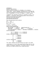
4.2.3 Setting Time Parameters.
The Q & A frame which prompts for time parameters is independent of
the mechanism which is to be simulated. However, the relevant
parameters to be set differ depending upon whether the mechanism
involves reactions depicted as rapid equilibria. If the mechanism does
not contain equilibrium steps, the following sort of display will appear
when the option “T” is chosen (the numbers shown are reasonable but
arbitrary):
Delta time:
1.0000E-03
Iterations/point:
1
Run time:
1.0000E+00
Ymax:
1.0000E+02
Flux tolerance:
1.0000E-01
Integral tolerance: 1.0000E-04
The “Delta time” is the time step used in the solution of the mechanism,
the “Iterations/point” defines the number of time steps per output
interval and the “Run time” is the total time course for the simulation.
The “Ymax” need only be set if a graphical output is to be used, in
which case it refers to the maximum value on the Y-axis of the graph.
The “flux tolerance” and “integral tolerance” are parameters which
control the numerical method used for the solution of the system. These
parameters determine how much computation will be required for the
solution, and so they should be set judiciously, as described below.
As in any technique of numerical integration, the solution of the
chemical differential equations proceeds by dividing the time axis into
intervals and using the derivatives at each discrete time point to
estimate the concentrations at the subsequent time point. The user will
specify a time interval for the output of simulated values (the “Delta
time” multiplied by the “Iterations/point”). However, if the
integration interval is too large, the numerical solution may verge out
PERFORMING A KINETIC SIMULATION
Page 4-4
of bounds. To prevent this, the program may carry out the integration
of several smaller time steps until the user-specified time interval has
passed. The division of the time interval is internal to the numerical
solution routine and so is transparent to the user; output will still
occur at the intervals defined by the user. The integral tolerance and
flux tolerance parameters determine how the program performs the
adjustment of the integration time step.
If the integral tolerance is non-zero, the integration will be
performed using the so-called backward differentiation formulae, or
Gear’s method. A matrix of partial derivatives (which relates the
inter-dependence of the chemical concentration changes) is used to
determine the time step for the integration. In this case, the value of
the integral tolerance parameter determines the fractional error in any
concentration which will be tolerated by the numerical routine before an
error is declared. The time step is chosen so as to keep the estimated
fractional truncation error less than the integral tolerance value.
If the integral tolerance is set to zero, the integration will be
performed using an alternate method (flux-tolerance) which uses a
chemical criterion to assure that the integration remains within bounds.
When the flux-tolerance method is in use, the flux tolerance parameter
defines the maximum fraction by which any species’ concentration may
change in a single iteration. In this case, the integration time step
is chosen so as to keep the fractional concentration changes within the
specified range. The flux tolerance value may also come into use when
Gear’s method is enabled, but only in the case of a violation of mass
conservation. Gear’s method may, under certain circumstances (for
example when a concentration is dropping very steeply) give rise to
negative concentrations. If such a mass conservation violation ensues,
the integration step is re-tried using a reduced integral tolerance, up
to 10 times. Thereafter, the step is retried using the flux-tolerance
method. Since mass conservation is impossible unless the permitted flux
tolerance is greater than 100 percent, the situation will in general
remit and Gear’s method will be automatically re-enabled for subsequent
iterations.
In summary, the use of two numerical methods assures that the
system will stay in bounds in terms of numerical error (Gear’s method)
and also in terms of concentrations (flux tolerance method). The exact
settings of these control parameters requires a certain amount of
experimentation with each given system. Note: Reasonable default
values are 0.1 for “flux tolerance” and 0.001 for “integral tolerance”.
If the simulation mechanism contains equilibrium steps, the
numerical approach is different since the concentration changes
resulting from equilibria are fundamentally time-independent and thus
the table of partial derivatives is incomplete. For this reason Gear’s
method can not be used on a system involving equilibria. The
flux-tolerance method can be applied to the remaining system of
differential equations. However, it is likely to lead to an excessively
stringent solution and require a disproportionate amount of
computational time because the incomplete system of differential
equations will appear to be “stiff”. For this reason, when the
mechanism contains equilibria, the user may interactively enable and
PERFORMING A KINETIC SIMULATION
Page 4-5
disable the flux-tolerance control. The Q & A frame for the time
constants will appear as follows (the numbers shown are reasonable but
arbitrary):
Delta time:
1.0000E-03
Iterations/point:
1
Run time:
1.0000E+00
Ymax:
1.2000E-01
Flux tolerance:
1.0000E-01
Equilibrium rapid:
NO
The significance of the parameters are explained above, with the
exception of the “equilibrium rapid” switch. This switch, which may be
set as “YES” or “NO”, determines whether the flux-tolerance method is to
be used at each time step. In order to get rapid simulation, BE SURE<CR><LF>
TO SET THIS TO “YES”. If flux-tolerance is not enabled, the delta
time will be used directly as the integration time step. In the case of
a rapid equilibrium solution, only the constraints of mass conservation
will assure that the integration has not gone wildly out of bounds.
When routinely simulating a mechanism with equilibria, it is a good idea
to periodically repeat the simulation with the flux-tolerance check
enabled.
4.3
SAVING AND RESTORING PARAMETERS.
Provision is made for resuming a simulation session without the
need to go through the entire process of specifying all parameters. The
set of parameters which is to be restored at a later time must first be
saved in a file. Choosing option “S” (save parameters) will store the
present parameter set in a file, whose name is specified in the manner
described in appendix B. At any later time, these parameters can be
retrieved by chosing option “R” and specifying the name of the saved
file.
4.4
INCLUDING DATA.
Choosing option “I” (include data) will bring a prompt for the name
of a data file. The specified data set will be displayed or plotted
along with the simulated output, so that the simulated data may be
directly compared to real data.
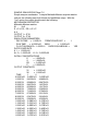
Once the specified file is opened, a prompt frame will appear which
will contain information about the data file including 1) the creator of
the file, 2) the time and date of its creation, 3) the maximum and
minimum values of the data, 3) the baseline, 4) the number of points in
the data set and 5) the maximum time of the data set.
PERFORMING A KINETIC SIMULATION Page 4-6
File: AD81N1301.DAT
File creator: BAB
Creation date: 14:05:43 13-NOV-81
Comments: AMPDAse 50.ug/ml : AMP 100.uM pH 6.5
DYmax : 1.1203E-01
DYmin: 2.0473E-03
Baseline: 1.9780E-03
Used : 1.9780E-03
Y range : 1.1011E-01
Used : 1.1011E-01
Npts :
1000
Used :
1000
Run time: 4.5000E+00
Used : 4.5000E+00
Correct file? (Y/N): YES
A prompt will be issued asking to verify that the file which was opened
is the correct one. If the reply is not “Y(es)”, it is assumed that the
wrong file has been opened, and the main menu will reappear. If the
reply is “Y(es)” followed by a <LF> or <ESC>, it is assumed that the
correct file has been opened and that the values displayed are to be
used without modification. In this case, the main menu will reappear
and the included data set will appear on all subsequent plots or
displays. If the answer is “Y(es)” followed by a carriage return, the
data display parameters may be set as described above in section 2.1.
In this case, the display parameters which may be changed include 1) the
baseline, 2) the range of the graphical ordinate, 3) the number of
points displayed and 4) the run-time, which allows the data to be
displayed on a different time-scale.
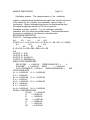
After including a data set, the Q & A frame for the time constants
will include three items of information regarding the data file. The
name of the data file will serve to remind the user of which experiment
is under consideration. Also the time maximum (“DTMAX”) and range of
values (“Y range”) for the data set will be displayed so that the
corresponding values for the simulation (“Run time” and “Ymax”) may be
chosen to agree. In fact, note that upon including a data set, these
simulation values are automatically set equal to the corresponding
values of the data set. An example of the time parameters Q & A frame
for a kinetic mechanism after the inclusion of a data file is shown
below:
Delta time:
1.0000E-03
Iterations/point:
1
Run time:
4.5000E+00 Data Tmax:
4.5000E+00
Ymax:
1.1011E-01 Data Y range:
1.1011E-01
Flux tolerance:
1.0000E-01
Integral Tolerance: 1.0000E-04
File name: AD81N1301.DAT
PERFORMING A KINETIC SIMULATION Page 4-7
4.4.1 Real Data And Simulated Data.
In general, the data file will contain the output of a stopped-flow
run which was generated by the STOPFLOW data acquisition program. The
format of a data file is shown in appendix D. In addition to real
stopped-flow data, it is possible to include simulated data, that is, to
superimpose one simulation on the output of a previous simulation. This
can be useful in comparing simulations made with different sets of
parameters or with entirely different mechanisms. The procedure is the
same as for inclusion of real data, but the file referenced is a file
previously generated by KINSIM itself through the “O” (output) option.
4.5
FITTING INCLUDED DATA.
Choosing option “A” (agreement to included data) will enable the
calculation of a sum-of-squares residual between one output channel of
the included data and the values of one output of the simulation. When
this option is active, the residual value will be displayed on the
screen at the end of each successfully completed simulation. The units
of the residual are defined by the simulated output; generally they are
concentration**2 per unit time per point. Note: This function is of
questionable usefulness when KINSIM is being run interactively. The
capability of calculating residual error is primarily intended to be
used when KINSIM is being run in supervised mode, under the control of
another program. The interactive user should rely upon visual
inspection to refine the estimates of simulation parameters. Enabling
option “A” will in general hinder the performance of a simulation,
particularly where KINSIM is implemented on a smaller computer (see
implementation notes, appendix E).
4.6
KINSIM OUTPUT OPTIONS.
There are several options for the output of the simulation. The output
may be displayed at the terminal in a graphic form, written as a
formatted text stream, written as an unformatted binary stream, or
rendered into a hard-copy plot. The main menu indicates which output
options are enabled at any given time.
4.6.1 Display.
This is the most common output option. The simulation will proceed
with all output to the terminal in graphic form. After the simulation
stops, the graph will remain displayed until the user types a <CR>. A
<Control-C> will bring up a textual display of the mechanism
superimposed upon the graphical output. Another <Control-C>, or a <CR>
will erase the textual display, leaving the graphical output, until a
<CR> is typed.
PERFORMING A KINETIC SIMULATION Page 4-8
4.6.2 List.
Choosing this option, a file is opened to receive the simulation
output as a text stream, so that it may later be typed or printed. If,
in response to the “Enter filename: “ prompt, the user enters “TT:”, the
text stream will not be written to a file at all, but will appear at the
terminal. Once the simulation is complete, the main menu will reappear.
Note: If the listing output is directed to the terminal, the display
option should be disabled. Spurious results may arise otherwise.
4.6.3 Plot.
The “Plot” option generates the files necessary for a VERSAPLOT
hard-copy graph of the simulation. The “Plot” option is only active for
a single simulation. Refer to appendix C for instructions on printing
the plots.
4.6.4 Output.
This option is used to generate an unformatted output file which
can be used to “Include”. This is the manner in which simulated data
files are created. terminal output. The “Output” option is active only
for a single simulation.
4.7
INTERRUPTIONS OF SIMULATION.
4.7.1 Elective Abortion.
If the time required to complete a simulation is unacceptably slow
or the user is simply impatient to reset parameters, the simulation may
be aborted at any point by typing a <Control-C>.
4.7.2 Simulation Errors.
A simulation may also be aborted due to errors. In the event of
such an error, a descriptive message will be displayed at the bottom of
the screen and the simulation will halt. Typing a <CR> will bring up
the main menu, and corrective measures may be taken. Refer to the
section on run time errors for suggestions of corrective measures.
PERFORMING A KINETIC SIMULATION Page 4-9
4.8
RUN TIME ERRORS.
In the present context, fatal errors refer to errors which will
halt a simulation run. Catastrophic errors refer to those which will
halt the program execution. Initialization errors refer to those which
are detected before a simulation begins and which prohibit the run from
being started.
4.8.1 Initialization Errors.
These errors generally arise if a required parameter is not set. A
descriptive message will be given and in general the corrective measure
is self-evident. For example, if the delta time is zero, the message
“Set delta time” will appear and the run will be prevented until it is
set to a non-zero value. An initialization error may arise if the
binary output option is enabled and the number of points would exceed
the maximum number of points permissable in an output file. In this
case, one should try to increase the delta time or, if that is not
permissable, increase the iterations/point.
4.8.2 Fatal Errors.
4.8.2.1
Mass Conservation Errors. Probably the most likely simulation error will be violation of mass
conservation. The situation can be alleviated by either using a smaller
integration time interval or a larger flux or integral tolerance. If
the time interval is decreased, it may be desirable to increase the
iterations/point so as to maintain the same output interval.
4.8.2.2
Integration Errors. Rarely an error may arise if Gear’s algorithm fails. In such an
instance, increasing the integral tolerance may remedy the situation.
If this fails, the integral tolerance may be set to zero so as to
activate the flux-tolerance method. If there is still a failure, it is
possible that the mechanism is written incorrectly.
4.8.2.3
Floating Overflow And Divide-by-zero Errors. Occasionally, a calculation may give rise to a value which is
beyond the range able to be represented by the computer. In particular,
the Gear algorithm may give rise to floating overflow errors when the
partial derivatives are calculated if the concentration changes of
certain species in the mechanism are strongly interdependent and the
magnitude of certain rate constants is relatively large. Decreasing the
magnitude of the rate constants may remedy the situation. Similarly,
PERFORMING A KINETIC SIMULATION
Page 4-10
certain sets of parameters may (rarely) give rise to a floating divideby-zero error. In the latter case, it is possible that the integral
tolerance should be lowered. Alternatively, with both these conditions,
the integration tolerance may need to be set to zero so as to activate
the flux-tolerance method. If it is not possible to perform the
simulation with rate constants which the user considers to be
“realistic”, it may be that the limitations of the computer simply do
not permit the simulation, in which case the mechanism must be
simplified.
4.8.2.4
Excessive Computation. If the amount of computation exceeds installation-defined limits
(see E.2), the simulation will halt with an error message indicating
that the iteration limit exceeded. At the WUMS-BCCF there is no limit
on computation for interactive use of the simulator, since the user has
the recourse to stop the simulation with a <Control-C> at any time.
4.8.3 Catastrophic Errors.
A catastrophic error could only arise for a completely unforeseen
reason. If KINSIM terminates with a system error message, faithfully
record the message and ask your system manager for advice.
APPENDIX A
ABBREVIATIONS AND SPECIAL SYMBOLS USED.
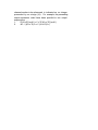
1.
Character codes.
1.
<CR> or <Return> : The carriage return key.
2.
<LF>: The line feed key.
3.
<ESC>: The escape key.
4.
<BS>: The backspace key.
5.
<Control-X>: The control-X character, where “X” may be any
character. Typed by depressing the control key and then,
while keeping the control key depressed, depressing the key
“X”.
2.
WUMS-BCCF: Washington University Medical School- Biological
Chemistry Computing Facility.
APPENDIX B
CONVENTIONS FOR SPECIFICATION OF FILES.
Several options will require the user to specify the name of a file
to be used for either output or input. Loading a mechanism, including
real data and restoring simulation parameters require an input file.
Writing a listing, outputting a simulated data file and saving
simulation parameters require an output file. The file name entered by
the user may consist of up to 40 characters in the standard record
management services file specification format:
( DEV:[DIR]NAME.EXT;VER ),
where DEV is a mnemonic representing the physical device, DIR the
directory on that device, NAME the file name, EXT the file type
(extension) and VER the version number of the file. The device and
directory may be omitted if the file may be assumed to reside in the
user’s current default directory; the version number defaults to the
highest existing version number of the specified file.
With all file name prompts issued by KINSIM, if there is an error
in opening the file specified, another prompt will be issued. If the
user subsequently gives up or decides not to open the file, typing
nothing except a <CR> will return the program to the main menu.
Each type of file has a default file type. If the file name is
entered without an extension, the appropriate file extension will be
assumed. The table below indicates the default file extensions for each
type of file:
File type
Default
Textual mechanism descriptor
.MEC
Binary mechanism descriptor
.SIM
Saved simulation parameters
.SAV
KINSIM-format data file
.SDF
Output listing file
.LST
APPENDIX C
AFTER THE SIMULATION SESSION.
(1)
After terminating session any listings may be typed or printed,
using the file names that were specified at the time they were
created:
$ TYPE listfilename
$ PRINT listfilename
(2)
Any VERSAPLOT output generated (option “P”) may be plotted
after terminating the session:
$ PLOT plotterlogicalname
In the present implementation, each plot consists of two files
of the same name but different extensions. The file name will
correspond to the VMS logical name for the logical device
“PLOTTER:”. The default file name is “VPLT”, but it may be
changed if, prior to beginning the simulation session the
logical name assignment is changed:
“$ ASSIGN PLOTTER: filename <CR>”.
The two files, of extension VPF and VVF corresond to the
VERSAPLOT parameter file and vector file, respectively.
Issuing the command
“$ PLOT filename <CR>”
will merge these files to create a raster which will be
automatically queued for printing on the device queue SYS$PLOT.
If multiple plots are made during the simulation session, they
will be separate pages of a single VERSAPLOT output.
APPENDIX D
DATA FILE STRUCTURE.
The data files for input to KINSIM may either be “real data” files,
produced by the STOPFLOW data acquisition program, or “simulated data”
files, produced by KINSIM itself. The files are written in large
fixed-length records, with each 512 byte record equivalent to one disk
block. The first record (block) of the file is a file header and
contains general information about the experiment. Subsequent blocks,
as needed, contain the data themselves. The data sections of real data
files are simply consecutive values of optical transmission or
absorbance recorded at fixed time intervals from the photomultiplier
tube of the stopped-flow apparatus. The data sections of the simulated
data files are more complex, owing to the fact that at each time point
there may be several output values. The simulated data, therefore, is
interdigitated; at each time point each of the output values is written
in turn.
DATA FILE STRUCTURE. Page D-2
D.1 THE DATA FILE HEADER STRUCTURE.
The first block of the data file contains the following
information:
FILECODE INTEGER*4 The file code identifies the file type
so that an incorrect file can not be
read by mistake.
CREATOR LOGICAL*1(10) The name (10 characters) of the experimenter
operating the stopped-flow may be recorded.
Simulated data files bear the name “ SIMUL “.
TIMEDATE LOGICAL*1(20) The time and date at the time of
creation of the file.
COMMENT LOGICAL*1(50) Up to 50 characters of comment
may be recorded.
RUNTIME REAL*4
The total time course of the run.
DELTAT REAL*4
The time interval between data.
SKIPCNT INTEGER*4 The number of time intervals between data
points. For real data files, SKIPCNT is
always equal to zero. For simulated data
files, SKIPCNT could be non-zero, but we
have never implemented such an option.
YMAX
REAL*4
The maximum data value.
YMIN
REAL*4
The minimum data value.
BASELINE REAL*4
The data baseline. For simulated data files,
BASELINE is always equal to zero. While the
baseline has meaning mostly for real data
files, adjusting the baseline to be used
in the display of simulated data files can
shift the curves along the Y-axis.
NUMBERPTS INTEGER*4 The number of data points. NUMBERPTS*DELTAT
should always equal RUNTIME.
OUTCNT
INTEGER*4 The number of output values at each
time point. For real data files produced by
the STOPFLOW program, OUTCNT always equals 1.
BTYPE
INTEGER*4 The type of data collection used in setting
the baseline (see STOPFLOW user’s guide).
This value is preserved only for archiving
purposes and is never used in the simulation.
CTYPE
INTEGER*4 The coversion type (absorbance/transmission).
As with BTYPE, an optional value.
EXPNSN
REAL*4
The expansion of the voltage scale from the
stopped-flow apparatus, expressed as EXPNSN
to 100 percent transmission. As with BTYPE,
an optional value.
DATA FILE STRUCTURE.
Page D-3
D.2 THE DATA STRUCTURE.
The data points are equally spaced in time, with the interval
DELTAT. At each time point, the value of each data set (up to MAXOUT
sets) is written in turn. For example, a data file consisting of three
sets of data (A, B and C) will be interdigitated thus:
A B C A B C ... A B C
0 0 0 1 1 1
m m m
where A represents the value of the first data set at time n*DELTAT.
n
D.3 CONVERTING DATA.
Two subroutines have been written which should be of great help in
creating suitable data files from sources other that the stopped-flow
apparatus and in altering data in existing KINSIM-format files. They
are named READDF and WRITEDF and serve as simple interfaces between the
casual programmer and the world of VAX-FORTRAN I/O. These subroutines
may be found in the object library SIMFIL.OLB, so that a data conversion
program may be linked with them by the command:
($) LINK MYPROGRAM,DRA1:[BARSHOP.SIMUL]SIMFIL/LIB.
A program to generate a data file might read a file in the appropriate
format might read in data from a file or as entered by a user from the
terminal. In any case, the program need only fill the array of data
values and call WRITEDF. For example:
DATA FILE STRUCTURE.
Page D-4
PROGRAM GENDF
! Skeleton program to
C
! generate data file.
PARAMETER
.
MAXPTS = 1024, ! These are the maximum
.
MAXOUT = 8
! dimensions of data array.
C
INTEGER lun
! Logical unit number
! of output file.
.
success
! Flag, where
! 1=successful, 0=failure.
C
CHARACTER filename*(*)
! The name of the output file.
C
INTEGER numberpts, skipcnt, outcnt !
REAL
runtime, deltat,
! File parameters
.
ymax, ymin, baseline,
! described above
.
yvals( MAXPTS, MAXOUT ) ! are declared.
CHARACTER creator *10,
!
.
comment *50,
!
.
timedate *20
!
INTEGER btype, ctype
!
REAL
expnsn
!
C
C Code begins here:
C
.
.
( File parameters are set and
the array yvals is filled. )
.
.
C
CALL WRITEDF
.
( MSGLVL, LUN, filename, success,
.
yvals, MAXPTS, MAXOUT,
.
creator, timedate, comment,
.
runtime, deltat, skipcnt, ymax, ymin, baseline,
.
numberpts, outcnt,
.
btype, ctype, expnsn )
C
IF ( success .EQ. 0 ) THEN
! Failure.
ELSE
.
.
.
Another application might be a program to alter the values in an
existing KINSIM-format file. As a simple example, consider a program to
multiply the values of a file by the factor 2.:
DATA FILE STRUCTURE.
PROGRAM MULTBY2
Page D-5
! Example program skeleton.
C
!
! Declarations as in preceding example.
!
C
C Code begins here:
C
CALL READDF
.
( MSGLVL, LUN, filename, success,
.
yvals, MAXPTS, MAXOUT,
.
creator, timedate, comment,
.
runtime, deltat, skipcnt, ymax, ymin, baseline,
.
numberpts, outcnt,
.
btype, ctype, expnsn )
C
DO 10 j = 1, outcnt
DO 10 i = 1, numberpts
10
yvals( i, j ) = yvals( i, j ) * 2.
C
CALL WRITEDF
.
( MSGLVL, LUN, filename, success,
.
yvals, MAXPTS, MAXOUT,
.
creator, timedate, comment,
.
runtime, deltat, skipcnt, ymax, ymin, baseline,
.
numberpts, outcnt,
.
btype, ctype, expnsn )
C
IF ( success .EQ. 0 ) THEN
! Failure.
ELSE
! Success.
END IF
END
Header comments from the routines follow.
DATA FILE STRUCTURE.
Page D-6
C
C The subroutines READDF and WRITEDF provide a convenient means to
C read and write data files in the KINSIM format. They return a status
C flag ( the INTEGER variable SUCCESS ), which is set to 1 for success
C or to 0 in the case of a failure.
C Messages may also be output by these routines, and the verbosity of
C the messages ( MSGLVL ) may be set to one of three levels:
C
Silent : No messages.
C
Terse : Error messages will be reported.
C
Verbose: Error, warning and success messages will be reported.
C Error message will be written to the
C default output device/file (SYS$OUTPUT:).
C
C READDF and WRITEDF require the calling program to allocate space for
C the storage of the file’s data. The array (YVALS) is the buffer for
C the data points (which are equally spaced in time). There
C may be more than one “channel” of data. That is, YVALS is a two dimC ensional array, and each channel is assumed to have the same number
C of points. Thus, the array YVALS is of dimension MAXPTS x MAXOUT,
C and YVALS(I,J) contains the I’th point of the J’th output channel.
C Declared dimensions of YVALS must be passed to READDF and WRITEDF
C (as the arguments MAXPTS and MAXOUT).
C
C The maximum number of channels permitted in a file and max number
C of points per channel are set by the parameters MAXPTSFIL and
C MAXOUTFIL in the subroutines READDF and WRITEDF.
C In the present implementation, MAXPTSFIL=1024 and MAXOUTFIL=8.
C For successful completion, MAXPTS must be .LE. MAXPTSFIL and
C MAXOUT must be .LE. MAXOUTFIL.
C
C
C
C LINKAGE INSTRUCTIONS:
C
C The function NEXTPT is part of the SIMFIL object library.
C The MACRO function ARGLOC is taken from M.T.Scott’s IO function
C library and is now also part of the SIMFIL object library.
C
C
C USAGE:
C
C
CALL WRITEDF
C
.
( MSGLVL, LUN, filename, success,
C
C
C
C
C
C
C
C
C
C
C
.
.
.
.
.
yvals, MAXPTS, MAXOUT,
creator, timedate, comment,
runtime, deltat, skipcnt, ymax, ymin, baseline,
numberpts, outcnt [,
arg1, ... , arg99 ] )
Input:
MSGLVL, LUN, filename,
creator, comment, runtime, deltat,
numberpts, outcnt, btype, ctype, expnsn,
yvals, MAXPTS, MAXOUT
DATA FILE STRUCTURE.
Page D-7
C
C
Optional input:
C
timedate ( If timedate is not passed,
C
present time and date will be written.
C
If passed, must be by %reference ).
C
arg1,..,arg99 ( Archiving parameters
C
may be written, if passed ).
C
Output: success
C
C
CALL READDF
C .
( MSGLVL, LUN, filename, success,
C .
[yvals], MAXPTS, MAXOUT,
C .
creator, timedate, comment,
C .
runtime, deltat, skipcnt, ymax, ymin, baseline,
C .
numberpts, outcnt [,
C .
arg1, ..., arg99 ] )
C
C
Input:
C
MSGLVL, LUN, filename,
C
MAXPTS, MAXOUT
C
Output:
C
creator, comment, runtime, deltat,
C
numberpts, outcnt, btype, ctype, expnsn,
C
success
C
C
Optional output:
C
yvals
( If yvals is not passed, only the
C
file header is read ).
C
arg1,...,arg99 ( These extra variables will be
C
filled iff passed ).
C
C DESCRIPTION OF ARGUMENTS:
C
C File IO parameters:
C MSGLVL - Controls verbosity of messages (INTEGER*4).
C
MSGLVL = 0->silent, =1->terse, =2->verbose.
C LUN
- The logical unit number of the data file (INTEGER*4).
C FILENAME - The name of the data file (CHARACTER*(*)).
C SUCCESS - Return status flag (INTEGER*4).
C
C Data array parameters:
C YVALS - The array of data ( REAL*4(MAXPTS,MAXOUT) ).
C MAXPTS - The “length” dimension of YVALS (INTEGER*4).
C MAXOUT - The “width” dimension of YVALS (INTEGER*4).
C
C Optional text arrays in file header:
C CREATOR - The name of the experimenter (CHARACTER*(*)).
C
The length of this string does not matter, but
C
at most, 10 bytes will be filled by READDF, and
C
at most, 10 bytes will be written by WRITEDF.
C TIMEDATE - Time and date of the file creation (CHARACTER*(*)).
C
As with CREATOR, TIMEDATE is truncated if.GT.20 byte.
C COMMENT - Associated comments for the file (CHARACTER*(*)).
C
As with CREATOR, COMMENT is truncated if.GT.50 bytes.
C
DATA FILE STRUCTURE.
Page D-8
C Required file parameters:
C RUNTIME - The duration of the experiment (REAL*4).
C DELTAT - The time-step between output intervals (REAL*4).
C SKIPCNT - The number of time steps skipped between pts (REAL*4).
C
In general, SKIPCNT is zero.
C YMAX
- The maximum datum in the file (REAL*4).
C
Used to scale graphical displays.
C YMIN
- The minimum datum in the file (REAL*4).
C
Used to scale graphical displays.
C BASELINE - The data baseline (REAL*4).
C NUMBERPTS- The number of data points (INTEGER*4).
C OUTCNT - The number of output channels ( number of points at
C
each time point ) (INTEGER*4).
C
C Archiving parameters:
C ARG1, - Archiving parameters may be included. They are
C
. - completely optional and may simply be left off of the
C
. - argument list. If passed, however, they must be
C ARG99 - 4 byte variables ( REAL*4 or INTEGER*4 or LOGICAL*4 ).
C
C The first three archiving parameters have been routinely in use
C for stopped-flow files, and they are explained below:
C
C BTYPE - For archiving only. A code, representing type of baseC
line collected in stopped-flow experiment (INTEGER*4).
C
BTYPE : 0=no baseline, 1=pretrigger,
C
2=uninterrupted, 3=interrupted.
C CTYPE - For archiving only. A code, representing type of optical
C
conversion of data (INTEGER*4).
C
CTYPE : 0=Transmission, 1=Absorbance.
C EXPNSN - For archiving only. Represents the response of the
C
photomultiplier tube, where a full scope-face’s
C
voltage represents EXPNSN to 100% optical transmission.
C
The electronics which we use allow for recording with
C
EXPNSN = 0., 50., 80., 90., or 95.
C
APPENDIX E
IMPLEMENTATION NOTES.
E.1
MODULE NOTES.
The program is modularized so that hopefully no editing will be required
on the big modules. Note:
I) I expect the kinetic compiler, KINCOMP.FOR, to run with very
few modifications on almost any computer. Probably the only
thing to change is the routine to open files (FILOPN).
II) SIMUL.FOR, SOLVE.FOR and LODMEC.FOR, which are the heart of the
run-time program should not require significant changes either.
Thus, you should be able to almost immediately run the program
to generate listed output.
III) GRAPHIC.FOR also should be fully portable as it is written.
However, the routines in GRAPHIC make calls to lower-level
routines for device-dependent operations.
1. Terminal-specific routines - The TRMSPCnnn.FOR module
contains the lower-level graphics routines. We presently
maintain two versions:
TRMSPC640 is for use with the PLOT10 graphics package
for use with the Digital Engineering VT640 terminal or
any terminal compatible with the Tektronix 4010 series.
TRMSPC125 is for use with the ReGIS graphics package
for use with the DEC VT125 terminal. Our TRMSPC125
module is essentially an emulator of a limited part of
the PLOT10 package.
To prevent the output of graphics to the terminal
from becoming rate-limiting during program, the
terminal I/O operations should be buffered. The
PLOT10 package has this feature built-in. To
emulate this feature of PLOT10, we have written the
routines found in TTOUTBUF.FOR. While TRMSPC125
should be comparatively easy to modify so as to
conform with any DEC FORTRAN dialect, the TTOUTBUF
routines which it calls will require more work.
IMPLEMENTATION NOTES. Page E-2
Note: The TRMSPC125 module is easily modified to
operate on the DEC VK100 (GIGI) terminal.
2. Plotter-dependent routines - The GRAPHIC module has low
level routines for hard-copy plotting which are written to
be compatible with the VERSAPLOT/CALCOMP software package.
Although the software packages mentioned above are widely used,
if you have other graphic routines, plotter calls in the
GRAPHIC and module may have to be changed and a different
TRMSPCnnn module may need to be written.
IV) QATRAN.FOR and QASCRN.FOR correspond to the “portable” and the
“in-house” version of the question-and-answer module described
in the user’s manual and each has its own conventions for
numeric entry. They contain routines to be called from PROMPT.
Either one or the other is to be linked with KINSIM. If QASCRN
is used, you must also be able to use (or replace) the
GETVALS.FOR routines.
V) UTIL.FOR has two essential routines which must be provided to
open and close files (FILOPN and FILCLS). Also note that the
routine GETMOD is optional—if the program will be run only
in interactive mode, simply set MODE = INTRCT.
VI) FILEIO.FOR is probably the most idiosyncratic module. What you
replace it with depends upon what sort of data file structure
you elect to use.
VII) The module QIOAST.FOR is concerned with the asynchronous
interception of a control-C typed by the user. It is entirely
VAX-specific (although it could easily be modified for use on
any of the PDP-11 family of computers). If you do not use it,
you have two choices:
1. Remove all references to ASTSET and ASTYES from the other
modules.
2. Replace the routines with stubs (RETURN, END), except for
the logical function ASTYES which should just return value
.FALSE.. If you do this, you will have less editing to
perform on the bigger modules.
E.2
INCLUDEd files and PARAMETERs.
There are several INCLUDE statements throughout the code. These
statements direct the FORTRAN compiler to read the contents of a
specified file as if that file were “in-line” code. The INCLUDE
statements enable one to change COMMON allocation of the programs by
changing a single file. For example, there is one file which is
IMPLEMENTATION NOTES.
Page E-3
INCLUDEd in every main module of KINCOMP (COMPAR.CMN) which contains the
parameters which determine the size of the program’s COMMON arrays.
There are several INCLUDE’d files for the simulator, one which sets the
corresponding dimension parameters (SIMPAR.CMN), and also one file for
each COMMON block. The frequent INCLUDE statements may need to be
changed to the appropriate syntax for other FORTRAN compilers. If your
version of FORTRAN does not have a statement analogous to INCLUDE, you
will have to edit the FORTRAN source files and replace each INCLUDE
statement with the contents of the specified file. If your FORTRAN
compiler does not support the PARAMETER statement, then you will have to
replace the appropriate numerical value at each occurance of the
parameter symbols throughout the code. If your FORTRAN compiler does
support the PARAMETER statement but does not allow parameters to be
defined in terms of previously defined parameters, you will have to
alter the file COMPAR.CMN so that the PARAMETER statements all have
numerical values to the right of the equal signs.
Most parameters relate to the storage requirements of KINSIM. One other
parameter which is important to note when installing the system is the
iteration limit MAXITR. This parameter sets the maximum number of steps
allowed within a single output interval (Delta time times Iterations per
point). When that number of iterations is exceeded (by either Gear’s
method or the flux tolerance method), the simulation will be halted (see
section 4.8.2.4). This parameter is only important if your installation
does not have a means of asynchronously aborting a run (e.g. Control-C,
see E.1.VII). In order to allow limitless computation, MAXITR should be
set to zero.
E.3
STORAGE REQUIREMENTS OF KINSIM.
The amount of memory required by KINSIM will vary depending upon the
maximum mechanism complexity. At the time of installation, you should
determine what limits you would like to establish for the maximum case.
On a smaller computer, memory limitations may require that the KINSIM
code be overlaid. The irreducible storage requirements will be
determined by the number of variables held in the KINSIM COMMON blocks.
The implementation-adjustable variables are:
M = MAXSPC = max number of species.
N = MAXRXN = max number of reactions.
O = MAXCPX = max number of equilibrium complexes.
P = MAXCPT = max number of equilibrium components.
Q = MAXAT1 = max number of species to be held at fixed concs
(species with mass conservation attribute [1).
R = MAXOUT = max number of output expressions.
S = MAXISX = max number of “reverse Polish” output calculation
instructions.
T = MAXFAC = max number of adjustable output factors for
output expressions.
U = MAXVAL = max number of fixed constant numerical values for
output expressions.
V = MAXNML = max number of characters in a symbolic name.
IMPLEMENTATION NOTES.
Page E-4
These variables correspond to the parameters in the file SIMPAR.CMN.
They may be changed simply by altering the contents of that single file,
and then rebuilding the KINSIM program.
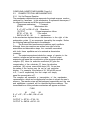
The complete expression for the COMMON storage requirements is:
Storage (bytes) = aM + bM**2 + cN + dNM +
eO + fO**2 + gOP + hQ +
iR + jS + kT + l.
The coefficients are expressed in terms of the system-dependent
parameters for data storage:
a = 2*INT + 22*DBL + V*CHR
b = 1*DBL
c = 5*INT + 2*DBL
d = 6*INT
e = 3*INT + 1*DBL
f = 1*INT
g = 1*INT
h = 1*INT
i = 2*INT + 1*DBL
j = 3*INT
k = 1*DBL + V*CHR
l = 71*INT + 13*LOG + 80*CHR + 14*SNG + (53+U)*DBL
where
INT = Storage required for one integer number
SNG = Storage required for one single precision real number
DBL = Storage required for one double precision real number
LOG = Storage required for one logical variable
CHR = Storage required for one character.
General values for the system-dependent parameters are:
INT = 4, SNG = 4, DBL = 8, LOG = 4, CHR = 4.
The programs do not use the CHARACTER data type. Rather, symbolic names
are filled into INTEGER arrays. This is discussed further below.
Default values for the implementation-adjustable parameters as written
in the version of the program which we circulate are:
O = M, P = M, Q = M, R = 8, S = 150, T = 20, U = 20, V = 10.
With these values, the expression for storage requirements expressed as
a function of N and M becomes:
Storage (bytes) = 245*M + 16*M**2 + 36*N + 24*N*M + 4056.
Thus, for a case with a maximum of 20 reactions and 20 species, the
COMMON storage requirements would be around 26 kilobytes.
IMPLEMENTATION NOTES.
Page E-5
There may be additional overhead, however, depending upon what course is
adopted relating to the writing and reading of external data files. The
scheme for writing a data file which we have written (subroutine WRTDF
in module FILEIO) involves a buffered I/O scheme in which one block of
data is held in COMMON (FILBUF). This involves an additional allocation
for a block’s worth (PERREC) of single precision values. There may also
be overhead for the inclusion (reading) of external data (e.g. for
display superimposition). If the data is to be read into memory, there
must be sufficient allocation for MAXPTS*MAXOUT single precision values
(see Appendix A, discussion of data file structure). This overhead can
be avoided if the data is held in a file (e.g. a direct access file).
However, please note that in that case, enabling the run-time option
which calculates a sum-of-squares residual might seriously slow the
program execution, due to file I/O operations at each iteration.
If a single precision version of KINSIM is desired, the DOUBLE PRECISION
variables may be declared as REAL (also changing a few references of
intrinsic double precision functions, e.g. DABS). To calculate the
storage requirements of a single precision version of KINSIM, evaluate
the equation above with DBL= SNG.
E.3.1 Relationship Between KINCOMP And KINSIM.
The routine which directly interfaces KINCOMP and KINSIM is LODMEC. The
READ statements in LODMEC must correspond to the WRITE statements in
KINCOMP. If the storage parameters of KINCOMP or KINSIM are changed, it
is possible that the resultant mechanism descriptor files from KINCOMP
will be too large to fit in the memory of KINSIM. All records in the
mechanism descriptor file are preceeded with their lengths. LODMEC
checks for adequacy of its storage space at each READ, so that, in case
there is an inconsistency, the message “Mechanism Overflow” is issued,
and the mechanism descriptor file is rejected.
E.4
REPRESENTATION OF CHARACTER DATA.
As mentioned above, the characters of symbolic names are filled into
INTEGER arrays, rather than using CHARACTER or even LOGICAL*1 data
types. This is to assure maximal portability, independent of the word
size of the computer in question. The storage can be decreased somewhat
if the arrays to hold the symbolic names are declared as LOGICAL*1 or
CHARACTER data type. The greatest saving will actually be in the size
of the KINCOMP output file, rather than the dynamic memory.
Accordingly, a routine in the compiler named WRTASC is provided which
can write the text contained in an INTEGER array byte-wise into the
KINCOMP output file. Changing the character storage element in the
output file requires corresponding changes to be made in a few of the
KINSIM modules. At each place where a change is needed, a declaration
statement for an INTEGER variable should be replaced with the
corresponding LOGICAL*1 statement. At each of these places in the code,
the proper replacement line is provided (as a comment), and the places
are all demarcated by comment lines beginning “C*LOG+ ...” and
IMPLEMENTATION NOTES.
Page E-6
“C*LOG- ...”. If the FORTRAN compiler on your computer does allow
LOGICAL*1 data type, it is suggested that you implement these changes in
the following modules.
1. KINCOMP.FOR: WRTASC
2. COMMON INCLUDE FILES: NAMES.CMN, FNAME.CMN, RDFCOM.CMN
3. SIMUL.FOR: SIMUL, KINSIM, GETOPT, BADC, SIMERR, SHOWM, OCALC
4. PROMPT.FOR: PUTTFS, PUTRDI, TFLAB, RDFLAB
5. QATRAN.FOR: CSCRN1, FSCRN1, GET1TF, GET1RP, YESNO
6. STRINGS.FOR: FILL, LINLEN, MOVC, UPCASE, SAME, IFIND
7. UTIL.FOR: FILOPN, HANDL
8. SOLVE.FOR: SOLVE, DGEAR, LUDATF
9. GRAPHIC.FOR: PLTHD
A method to do this automatically is outlined at the end of the next
section.
E.5
HEADER NOTES. EXTRACTING AND SUPPRESSING SECTIONS OF CODE.
The in-line header comments in all the modules contain synoptic
information which will be of use in understanding the system. Since the
header notes are delineated by comment lines beginning with “C*+” and
“C*-“, it is a simple matter to extract them, using a program like the
following:
PROGRAM EXTCOM
! Extracts header notes.
C
CHARACTER LINE*80
LOGICAL*1 COPY /.FALSE./
INTEGER*4 EOF /0/
C
WRITE (*,’(‘’ Enter name of source file: ‘’,$)’)
READ (*,’(A80)’) LINE
OPEN (UNIT=1,NAME=LINE,TYPE=’OLD’)
WRITE (*,’(‘’ Enter name of output file: ‘’,$)’)
READ (*,’(A80)’) LINE
OPEN (UNIT=2,NAME=LINE,TYPE=’NEW’)
C
DO WHILE (EOF .EQ. 0)
READ (1,’(Q,A)’,IOSTAT=EOF) LENGTH,LINE
IF (EOF .EQ. 0) THEN
COPY=(COPY .OR.(LINE(1:3).EQ.’C*+’.OR.LINE(1:3).EQ.’c*+’))
IF (COPY) WRITE (2,’(1X,A)’) LINE(1:LENGTH)
COPY=(COPY.AND.(LINE(1:3).NE.’C*-‘.AND.LINE(1:3).NE.’c*-‘))
END IF
END DO
END
A copy of these notes should be attached in appendix H. Among the
information included in the header notes is the list of calls and
references made by each routine. This information is required if a
linkage overlay scheme is needed.
IMPLEMENTATION NOTES. Page E-7
A similar program can be used to change the required sections of
FORTRAN source code for implementing the LOGICAL*1 version of the
program, something like the following:
PROGRAM CVTLI ! Converts code to logical*1 or integer versions.
C
CHARACTER LINE*80
INTEGER*4 IOS /0/
LOGICAL INT/.FALSE./, LOG/.FALSE./
INTEGER INTMOD/0/, LOGMOD/1/, MODE/-1/
C
WRITE (6,’(‘’ Enter name of source file: ‘’,$)’)
READ (5,’(A80)’) LINE
OPEN (UNIT=1,NAME=LINE,TYPE=’OLD’)
WRITE (6,’(‘’ Enter name of output file: ‘’,$)’)
READ (5,’(A80)’) LINE
OPEN (UNIT=2,NAME=LINE,TYPE=’NEW’)
C
WRITE (6,’(‘’ Convert to LOGICAL*1(L) or INTEGER(I): ‘’,$)’)
READ (5,’(A)’) LINE
IF (LINE(1:1).EQ.’I’ .OR. LINE(1:1).EQ.’i’) MODE = INTMOD
IF (LINE(1:1).EQ.’L’ .OR. LINE(1:1).EQ.’l’) MODE = LOGMOD
C
DO WHILE (IOS .EQ. 0)
READ (1,’(Q,A)’,IOSTAT=IOS) LENGTH,LINE
IF (IOS .EQ.0) THEN
IF (LINE(1:6).EQ.’C*INT+’) THEN
INT = .TRUE.
LOG = .FALSE.
ELSE IF (LINE(1:6).EQ.’C*INT-‘) THEN
INT = .FALSE.
ELSE IF (LINE(1:6).EQ.’C*LOG+’) THEN
LOG = .TRUE.
INT = .FALSE.
ELSE IF (LINE(1:6).EQ.’C*LOG-‘) THEN
LOG = .FALSE.
ELSE
IF (INT) THEN
IF (MODE .EQ. LOGMOD) THEN
IF (LINE(1:1).NE.’C’) LINE(1:1) = ‘C’
ELSE IF (MODE .EQ. INTMOD) THEN
IF (LINE(1:1).EQ.’C’) LINE(1:1) = ‘ ‘
ENDIF
ELSE IF (LOG) THEN
IF (MODE .EQ. INTMOD) THEN
IF (LINE(1:1).NE.’C’) LINE(1:1) = ‘C’
ELSE IF (MODE .EQ. LOGMOD) THEN
IF (LINE(1:1).EQ.’C’) LINE(1:1) = ‘ ‘
ENDIF
ENDIF
ENDIF
WRITE (2,’(1X,A)’) LINE(1:LENGTH)
END IF
END DO
END
IMPLEMENTATION NOTES.
Page E-8
A similar scheme can be used to enable and disable VAX-specific and
RT-11-specific sections of files GETVALS.FOR, KINCOMP.FOR, QIOAST.FOR
and UTIL.FOR, using the delineators “C*VAX+”, “C*VAX-“, “C*RT1+”,
“C*RT1-“.
E.6
PROGRAM FLOW AND OVERLAYING.
The programs are modularized in accordance with their flow, so as to
facilitate overlaying. The following diagrams should be useful in
designing an overlay scheme. These diagrams relate the root segments
for each stage during the running of the compiler and simulator. The
entire list of subroutines needed in the branches can be determined from
the lists of calls in the header notes.
|
||
|
| RCTALZ | EQCOMP | GENEQB | MAKMDB |
||--------|||--------|||--------|||--------||
|
KINCOMP
|
||
COMPILER Program Flow.
|
|
|
|
|
|
|
|
|----------|
|
|
|
|
|
|
|
| INIT | LODMEC | PRESIM | DOSIM | FINSIM |
||--------|||--------|||--------|||--------|||--------||
|
KINSIM
|
||
SIMULATOR Program Flow.
E.7
GRAPHICS ROUTINES NOT PROVIDED.
As mentioned above, the routines in the GRAPHIC module make
references to VERSAPLOT and PLOT10 subroutines.
1.
VERSAPLOT subroutines: All the referenced routines conform to
conventional pen plotter descriptions.
Subroutine PLOTS (ibuf,nloc,ldev) - Used to initialize the
plotter system. The arguments are meaningless in newer
versions of VERSAPLOT.
Subroutine PLOT (x,y,ipen) - Processes straight line “pen”
moves with the pen either up or down during movements.
IMPLEMENTATION NOTES. Page E-9
. x and y are coordinates defining the terminal position
of the “pen” move.
. ipen is a signed integer controlling the “pen” up/down
status, reorigin, and end of plot requests. In this
context, all that is needed is:
. ipen = +3: Move to (x,y).
. ipen = +2: Draw to (x,y).
. ipen = -999: End of plot.
. ipen = +999: End of plot, terminate all plotting.
Subroutine WHERE (xnow, ynow, dfact) - Returns the present
“pen” position and the drawing ratio factor.
Subroutine SYMBOL (x,y,height,itext,angle,nc) - Plots
alphanumeric annotations at various angles and sizes.
Subroutine NUMBER (x,y,height,realnumber,angle,ndec) Converts a floating point number to decimal equivalent and
draws it on plot. Refer to subroutine NUMBRE in GRAPHIC
module.
2.
PLOT10 subroutines: The terminal graphics routines are called
in accordance with the PLOT10 conventions. All routines to
emulate the required subset of PLOT10 are provided for the
VT125 (in module TRMSPC125). If you are implementing terminal
graphics on a system which uses another terminal and you do not
have a PLOT10-compatible package, the following routines must
be written.
Subroutine INITT640 (ibaud) - Initializes terminal and
terminal control system (including establishment of output
buffering, as in TTOUTBUF module). Clears screen, sets
terminal into graphics mode and homes graphics cursor.
Subroutine VWINDO (xmin,xrange,ymin,yrange) - Defines the
physical coordinates of the terminal screen in terms of
vitrual coordinates, extending horizontally from xmin to
xmin+xrange and vertically from ymin to ymin+yrange.
Subroutine MOVEA (x,y) - Moves graphics cursor to virtual
coordinates (x,y).
Subroutine DRAWA (x,y) - Draws straight line from present
virtual coordinates to virtual coordinates (x,y).
Subroutine POINTA (x,y) - Moves to virtual coordinates
(x,y) and draws one point there.
Subroutine HOME - Moves graphics cursor to “home” position
(upper left).
Subroutine ANCHO (ichar) - Enters alphanumeric mode (if
necessary), outputs an alphanumeric character at present
coordinates. Input argument is a 7-bit ASCII, non-control
character which is right-justifiedwithin an integer word.
Subroutine TSEND - Flushes all pending buffered graphics
output.
IMPLEMENTATION NOTES. Page E-10
E.8
INSTALLATION SUMMARY.
1.
First adjust the INCLUDEd files and PARAMETER statements, as
needed (see E.2 and E.3).
2.
For the initial installation, use the simpler transportable Q&A
package, QATRAN, especially if not on a DEC computer system
(see E.1.IV).
3.
If not using a VAX computer, replace the ASTYES function
(QIOAST) (see E.1.VII).
4.
Likely alterations will be needed in:
1.
FILOPN function (see E.1.I) and subroutine WRTASC (see E.4)
in KINCOMP.
2.
UTIL module of KINSIM.
3.
GRAPHIC module of KINSIM (see E.1.III and E.7).
4.
FILEIO module of KINSIM (see E.1.VI).
5.
Also, if changing to a version using LOGICAL*1 character
storage, perform the simple alterations outlined in E.4.
6.
If required, design a linkage overlay descriptor (see E.6).
7.
Build the system:
$ FORTRAN KINCOMP
$ LINK KINCOMP
$ FORTRAN SIMUL, SOLVE, QIOAST, UTIL, GRAPHIC, LODMEC,
STRINGS, FILEIO, PROMPT, Q&A-routines, TRMSPCnnn
$ LINK/EXE=KINSIM SIMUL, SOLVE, QIOAST, UTIL, GRAPHIC,
LODMEC, STRINGS, FILEIO, PROMPT, Q&A-routines, TRMSPCnnn,
PLOT10-system, VERSAPLOT-system
where Q&A-routines refer to either simply QATRAN or the two
modules QASCRN and GETVALS (see E.1.IV), and TRMSPCnnn refers
to either the TRMSPC640 module (if using a PLOT10-compatible
terminal), TRMSPC125 (if using a VT125), or the appropriate
terminal-dependent routines for your terminal. The required
components of the PLOT10-system and VERSAPLOT-system are
discussed in section E.7.
APPENDIX F
SAMPLE SIMULATIONS
After the system is installed, it is advisable to do extensive
“shake down”. Several examples, plausible and im-, should be tried.
Note the few examples scattered throughout this document. The first
sort of mechanisms to try are the simplest, to assure that the
compilation and numerical processes are operating correctly. For
example, a mechanism like the following tests for correct solution of
both a first and second order reaction:
First and second order reactions.
MECHANISM DESCRIPTOR
First order and second order reactions.
K+1
K+2
A == B ; 2C == D
K-1
K-2
OUTPUT 1 = %(A0/A)
OUTPUT 2 = #1/C-#1/C0
SIMULATION PARAMETERS
DELTA TIME = 1.000D-02
ITERATIONS/POINT =
1
RUN TIME
= 1.000D+00
YMAX
= 1.000D+00
FLUX TOLERANCE = 1.000D-01
INTEGRAL TOLERANCE = 1.000D-05
RATE CONSTANTS
K+ 1 = 1.000D+00 K- 1 = 0.000D+00
K+ 2 = 1.000D+00 K- 2 = 0.000D+00
INITIAL CONCENTRATIONS
A
= 1.000D+00
B
= 0.000D+00
C
= 1.000D+00
D
= 0.000D+00
OUTPUT CONSTANTS
A0
= 1.000D+00
C0
= 1.000D+00
The output constants A0 and C0 being set equal to the initial
concentrations of A and C, both outputs must be linear with time, with
slopes of one and two, respectively. You should confirm for yourself
that this is true (within truncation error, Integral tolerance).
SAMPLE SIMULATIONS Page F-2
Simple enzyme mechanism. A simple Michaelis-Menten enzyme reaction
such as the following uses both kinetic and equilibrium steps. With the
“List” option, the output should match the following:
MECHANISM DESCRIPTOR
Michaelis-Menten reaction.
K1
K+2
E + S = ES ; ES == E + P
K-2
OUTPUT 1 = S*X1
OUTPUT 2 = P*X2
SIMULATION PARAMETERS
DELTA TIME = 1.000D-01
ITERATIONS/POINT =
1
RUN TIME
= 4.500D+00
YMAX
= 1.200D+02
FLUX TOLERANCE = 1.000D-01
RAPID EQUILIBRIUM =
YES
RATE CONSTANTS
K 1 = 1.000D+02
K+ 2 = 1.000D+02 K- 2 = 0.000D+00
INITIAL CONCENTRATIONS
E
= 1.000D+00
S
= 1.000D+02
ES
= 0.000D+00
P
= 0.000D+00
OUTPUT CONSTANTS
X1
= 1.000D+00
X2
= 1.000D+00
TIME
1
2
0.000E+00 9.950E+01 0.000E+00
1.000E-01 9.453E+01 4.988E+00
2.000E-01 8.968E+01 9.847E+00
3.000E-01 8.497E+01 1.457E+01
4.000E-01 8.039E+01 1.917E+01
5.000E-01 7.594E+01 2.362E+01
6.000E-01 7.164E+01 2.794E+01
7.000E-01 6.748E+01 3.211E+01
8.000E-01 6.347E+01 3.614E+01
9.000E-01 5.960E+01 4.003E+01
1.000E+00 5.588E+01 4.376E+01
1.100E+00 5.231E+01 4.735E+01
1.200E+00 4.889E+01 5.078E+01
1.300E+00 4.562E+01 5.406E+01
1.400E+00 4.250E+01 5.720E+01
1.500E+00 3.954E+01 6.018E+01
1.600E+00 3.672E+01 6.301E+01
1.700E+00 3.405E+01
1.800E+00 3.152E+01
...
...
...
6.570E+01
6.824E+01
SAMPLE SIMULATIONS
Page F-3
Oscillating systems. The representations of the oscillating
systems (example textual mechanism descriptor files 3 and 4) at the end
of the section on the compiler are particularly rigorous tests of
functionality. Before attempting these tests, be forewarned that they
will require a significant amount of CPU time to perform.
Feedback activation oscillator. Try the feed-back activation
simulation with the values as specified below. There should be about
two cycles of oscillation in 1.8 seconds of simulation time.
MECHANISM DESCRIPTOR
OSCIL1P1 - Oscillating system, N=1, P=1.
K+1
K2
K+3
K4
K+5
POOL[1 == A ; A + E = EA ; EA == E + B ; B + F = FB ; FB == F + SINK[1
K-1
K-3
K-5
K6
K7
K+8
E + B = EB ; A + EB = EBA ; EBA == B + EB
K-8
OUTPUT 1 = A*X1
OUTPUT 2 = B*X2
OUTPUT 3 = (E+EA)*X3
OUTPUT 4 = (EB+EBA)*X4
SIMULATION PARAMETERS
DELTA TIME = 1.000D-02
ITERATIONS/POINT =
3
RUN TIME
= 1.800D+00
YMAX
= 1.200D+02
FLUX TOLERANCE = 1.000D-01
RAPID EQUILIBRIUM =
YES
RATE CONSTANTS
K+ 1 = 5.000D+00 K- 1 = 0.000D+00
K 2 = 1.000D+02
K+ 3 = 5.000D+00 K- 3 = 0.000D+00
K 4 = 1.000D+01
K+ 5 = 1.000D+03 K- 5 = 0.000D+00
K 6 = 1.000D+02
K 7 = 1.000D+01
K+ 8 = 2.000D+03 K- 8 = 0.000D+00
INITIAL CONCENTRATIONS
POOL[1 = 1.000D+02
A
= 0.000D+00
E
= 1.000D+00
EA
= 0.000D+00
B
= 0.000D+00
F
= 1.000D+00
FB
= 0.000D+00
SINK[1 = 0.000D+00
EB
= 0.000D+00
EBA
= 0.000D+00
OUTPUT CONSTANTS
X1
= 5.000D-01
X2
= 5.000D-01
X3
= 5.000D+01
X4
= 5.000D+01
SAMPLE SIMULATIONS
TIME
0.000E+00
3.000E-02
6.000E-02
9.000E-02
1.200E-01
1.500E-01
1.800E-01
2.100E-01
2.400E-01
2.700E-01
3.000E-01
3.300E-01
3.600E-01
3.900E-01
4.200E-01
4.500E-01
4.800E-01
5.100E-01
5.400E-01
5.700E-01
6.000E-01
6.300E-01
6.600E-01
6.900E-01
7.200E-01
7.500E-01
7.800E-01
8.100E-01
8.400E-01
8.700E-01
9.000E-01
9.300E-01
9.600E-01
9.900E-01
1.020E+00
1.050E+00
1.080E+00
1.110E+00
1.140E+00
1.170E+00
1.200E+00
1
2
0.000E+00
7.432E+00
1.487E+01
2.229E+01
2.971E+01
3.709E+01
4.443E+01
5.171E+01
5.887E+01
6.584E+01
7.248E+01
7.850E+01
8.335E+01
8.610E+01
8.543E+01
8.043E+01
7.153E+01
6.000E+01
4.712E+01
3.395E+01
2.156E+01
1.147E+01
5.602E+00
3.911E+00
3.843E+00
4.136E+00
4.586E+00
5.215E+00
6.108E+00
7.420E+00
9.409E+00
1.247E+01
1.697E+01
2.286E+01
2.954E+01
3.653E+01
4.359E+01
5.063E+01
5.755E+01
6.422E+01
7.046E+01
Page F-4
3
0.000E+00
2.290E-03
6.782E-03
1.279E-02
2.106E-02
3.288E-02
5.046E-02
7.781E-02
1.226E-01
1.998E-01
3.411E-01
6.146E-01
1.173E+00
2.347E+00
4.733E+00
8.943E+00
1.501E+01
2.234E+01
3.020E+01
3.786E+01
4.445E+01
4.860E+01
4.848E+01
4.419E+01
3.837E+01
3.242E+01
2.662E+01
2.106E+01
1.582E+01
1.100E+01
6.795E+00
3.487E+00
1.416E+00
5.221E-01
2.375E-01
1.550E-01
1.401E-01
1.598E-01
2.121E-01
3.134E-01
5.045E-01
4
5.000E+01
5.000E+01
4.998E+01
4.995E+01
4.991E+01
4.984E+01
4.974E+01
4.957E+01
4.929E+01
4.881E+01
4.793E+01
4.630E+01
4.327E+01
3.804E+01
3.064E+01
2.302E+01
1.730E+01
1.374E+01
1.179E+01
1.108E+01
1.163E+01
1.387E+01
1.755E+01
2.032E+01
2.212E+01
2.387E+01
2.584E+01
2.810E+01
3.075E+01
3.388E+01
3.760E+01
4.184E+01
4.575E+01
4.808E+01
4.899E+01
4.927E+01
4.928E+01
4.913E+01
4.880E+01
4.817E+01
4.703E+01
0.000E+00
4.957E-03
2.076E-02
4.823E-02
9.155E-02
1.584E-01
2.627E-01
4.301E-01
7.088E-01
1.193E+00
2.068E+00
3.698E+00
6.726E+00
1.196E+01
1.936E+01
2.698E+01
3.270E+01
3.627E+01
3.821E+01
3.892E+01
3.837E+01
3.613E+01
3.245E+01
2.968E+01
2.788E+01
2.613E+01
2.416E+01
2.190E+01
1.925E+01
1.612E+01
1.240E+01
8.159E+00
4.251E+00
1.920E+00
1.011E+00
7.328E-01
7.171E-01
8.679E-01
1.204E+00
1.830E+00
2.973E+00
1.230E+00
1.260E+00
1.290E+00
1.320E+00
1.350E+00
1.380E+00
1.410E+00
...
...
7.590E+01
7.987E+01
8.134E+01
7.911E+01
7.275E+01
6.306E+01
5.132E+01
...
8.766E-01
1.629E+00
3.164E+00
6.090E+00
1.083E+01
1.716E+01
2.442E+01
...
...
4.494E+01
4.122E+01
3.531E+01
2.788E+01
2.108E+01
1.631E+01
1.346E+01
5.062E+00
8.777E+00
1.469E+01
2.212E+01
2.892E+01
3.369E+01
3.654E+01
SAMPLE SIMULATIONS
Feedback activation oscillator, kinetic.
Page F-5
Compile the same
mechanism without equilibrium steps, as follows.
MECHANISM DESCRIPTOR
OSCIL1P1 - Oscillating system, N=1, P=1, Kinetic.
K+1
K+2
K+3
K+4
POOL[1 == A ; A + E == EA ; EA == E + B ; B + F == FB
K-1
K-2
K-3
K-4
K+5
K+6
K+7
K+8
FB == F + SINK[1 ; E + B == EB ; A + EB == EBA ; EBA == B + EB
K-5
K-6
K-7
K-8
OUTPUT 1 = A*X1
OUTPUT 2 = B*X2
OUTPUT 3 = (E+EA)*X3
OUTPUT 4 = (EB+EBA)*X4
SIMULATION PARAMETERS
DELTA TIME = 3.000D-02
ITERATIONS/POINT =
1
RUN TIME
= 4.500D+00
YMAX
= 1.200D+02
FLUX TOLERANCE = 1.000D-01
INTEGRAL TOLERANCE = 1.000D-03
RATE CONSTANTS
K+ 1 = 3.000D+00 K- 1 = 0.000D+00
K+ 2 = 1.000D-01 K- 2 = 1.000D+01
K+ 3 = 5.000D+00 K- 3 = 0.000D+00
K+ 4 = 1.000D+02 K- 4 = 1.000D+03
K+ 5 = 1.000D+03 K- 5 = 0.000D+00
K+ 6 = 1.000D+01 K- 6 = 1.000D+03
K+ 7 = 1.000D+02 K- 7 = 1.000D+03
K+ 8 = 2.000D+03 K- 8 = 0.000D+00
INITIAL CONCENTRATIONS
POOL[1 = 1.000D+02
A
= 0.000D+00
E
= 1.000D+00
EA
= 0.000D+00
B
= 0.000D+00
F
= 1.000D+00
FB
= 0.000D+00
SINK[1 = 0.000D+00
EB
= 0.000D+00
EBA
= 0.000D+00
OUTPUT CONSTANTS
X1
= 5.000D-01
X2
X3
X4
= 5.000D-01
= 5.000D+01
= 5.000D+01
SAMPLE SIMULATIONS
TIME
0.000E+00
3.000E-02
6.000E-02
9.000E-02
1.200E-01
1.500E-01
1.800E-01
2.100E-01
2.400E-01
2.700E-01
3.000E-01
3.300E-01
3.600E-01
3.900E-01
4.200E-01
4.500E-01
4.800E-01
5.100E-01
5.400E-01
5.700E-01
6.000E-01
6.300E-01
6.600E-01
6.900E-01
7.200E-01
7.500E-01
7.800E-01
8.100E-01
8.400E-01
8.700E-01
9.000E-01
9.300E-01
9.600E-01
9.900E-01
1.020E+00
1.050E+00
1.080E+00
1.110E+00
1.140E+00
1.170E+00
1.200E+00
1
2
0.000E+00
4.494E+00
8.978E+00
1.345E+01
1.792E+01
2.239E+01
2.684E+01
3.129E+01
3.573E+01
4.016E+01
4.458E+01
4.898E+01
5.337E+01
5.773E+01
6.207E+01
6.637E+01
7.064E+01
7.487E+01
7.903E+01
8.313E+01
8.714E+01
9.104E+01
9.481E+01
9.841E+01
1.018E+02
1.049E+02
1.078E+02
1.102E+02
1.121E+02
1.135E+02
1.141E+02
1.140E+02
1.129E+02
1.109E+02
1.078E+02
1.036E+02
9.836E+01
9.216E+01
8.509E+01
7.732E+01
6.906E+01
Page F-6
3
0.000E+00
2.280E-04
1.195E-03
3.107E-03
5.988E-03
9.777E-03
1.444E-02
2.000E-02
2.652E-02
3.411E-02
4.303E-02
5.347E-02
6.555E-02
8.035E-02
9.769E-02
1.185E-01
1.436E-01
1.744E-01
2.120E-01
2.590E-01
3.170E-01
3.898E-01
4.816E-01
5.972E-01
7.441E-01
9.318E-01
1.172E+00
1.481E+00
1.876E+00
2.380E+00
3.021E+00
3.828E+00
4.834E+00
6.072E+00
7.572E+00
9.353E+00
1.141E+01
1.374E+01
1.628E+01
1.895E+01
2.164E+01
4
5.000E+01
5.000E+01
5.000E+01
4.999E+01
4.999E+01
4.998E+01
4.997E+01
4.995E+01
4.994E+01
4.992E+01
4.989E+01
4.986E+01
4.982E+01
4.978E+01
4.973E+01
4.966E+01
4.958E+01
4.949E+01
4.937E+01
4.922E+01
4.904E+01
4.882E+01
4.854E+01
4.819E+01
4.776E+01
4.722E+01
4.655E+01
4.573E+01
4.472E+01
4.352E+01
4.210E+01
4.048E+01
3.866E+01
3.667E+01
3.459E+01
3.247E+01
3.038E+01
2.841E+01
2.661E+01
2.506E+01
2.379E+01
0.000E+00
2.601E-04
1.699E-03
5.099E-03
1.098E-02
1.955E-02
3.091E-02
4.525E-02
6.286E-02
8.403E-02
1.097E-01
1.404E-01
1.765E-01
2.215E-01
2.748E-01
3.393E-01
4.177E-01
5.136E-01
6.311E-01
7.769E-01
9.566E-01
1.181E+00
1.461E+00
1.807E+00
2.240E+00
2.780E+00
3.449E+00
4.274E+00
5.278E+00
6.482E+00
7.896E+00
9.523E+00
1.134E+01
1.333E+01
1.541E+01
1.753E+01
1.962E+01
2.159E+01
2.339E+01
2.494E+01
2.621E+01
1.230E+00
1.260E+00
1.290E+00
1.320E+00
1.350E+00
1.380E+00
1.410E+00
1.440E+00
...
...
6.053E+01
5.202E+01
4.380E+01
3.619E+01
2.947E+01
2.389E+01
1.958E+01
1.658E+01
...
2.420E+01
2.646E+01
2.820E+01
2.920E+01
2.928E+01
2.826E+01
2.615E+01
2.306E+01
...
...
2.285E+01
2.228E+01
2.211E+01
2.240E+01
2.318E+01
2.442E+01
2.610E+01
2.819E+01
2.715E+01
2.772E+01
2.789E+01
2.760E+01
2.682E+01
2.558E+01
2.390E+01
2.181E+01
APPENDIX G
MAINTENANCE.
Chemical Kinetic Simulation System.
Washington University Medical School
Department of Biological Chemistry
THE INFORMATION ON THIS TAPE IS SUBJECT TO CHANGE WITHOUT NOTICE
AND
SHOULD THEREFORE NOT BE CONSTRUED AS A COMMITMENT BY THE
AUTHOR, HIS
DEPARTMENT, OR HIS SCHOOL. THE AUTHOR ASSUMES NO RESPONSIBILTY
FOR
USE OR RELIABILTY OF THIS SOFTWARE UNDER ANY CIRCUMSTANCES.
Actually, questions and suggestions are welcome.
If you have any problems or insights, please contact us.
Prof. Carl Frieden
Department of Biological Chemistry
Box 8231
Washington University School of Medicine
St. Louis, Missouri 63110
Telephone: 314-362-3344
Good luck, and enjoy!
APPENDIX H
HEADER NOTES.
In this place, the header notes should be attached.
Page Index-1
INDEX
Binary mechanism descriptor . . . . 3-1
Data file . . . . . . . . . . . . . D-1
converting . . . . . . . . . . . . D-3
READDF . . . . . . . . . . . . . D-3, D-5
WRITEDF . . . . . . . . . . . . D-3, D-5
data structure . . . . . . . . . . D-3
generating
WRITEDF . . . . . . . . . . . . D-3
header structure . . . . . . . . . D-2
Implementation . . . . . . . . . . . E-1
Installation . . . . . . . . . . . . E-1
compiler . . . . . . . . . . . . . E-1
header notes . . . . . . . . . . . E-6, H-1
overlaying . . . . . . . . . . . . E-8
simulator . . . . . . . . . . . . E-1
file i/o . . . . . . . . . . . . E-2
graphics . . . . . . . . . . . . E-1 to E-2, E-8
buffered i/o . . . . . . . . . E-1
storage . . . . . . . . . . . . . E-3
KINCOMP
description . . . . . . . . . . . 3-1
error codes . . . . . . . . . . . 3-9
operation . . . . . . . . . . . . 3-1
KINSIM
Control-C . . . . . . . . . . . . 4-2, 4-7 to 4-8, E-2
errors . . . . . . . . . . . . . . 4-8
including data . . . . . . . . . . 4-5
fitting . . . . . . . . . . . . 4-7
interruptions of simulation . . . 4-8, E-3
loading mechanism . . . . . . . . 4-1
menu . . . . . . . . . . . . . . . 4-1
output options . . . . . . . . . . 4-7
display . . . . . . . . . . . . 4-7
list . . . . . . . . . . . . . . 4-8, C-1
output . . . . . . . . . . . . . 4-8
plot . . . . . . . . . . . . . . 4-8, C-1
saving and restoring parameters . 4-5
setting parameters . . . . . . . . 4-2
integration constants . . . . . 4-4
equilibrium . . . . . . . . . 4-4
Q & A frames . . . . . . . . . . 4-2
in-house . . . . . . . . . . . 4-2, E-2
portable . . . . . . . . . . . 4-3, E-2
time constants . . . . . . . . . 4-3
Mass conservation . . . . . . . . . 3-2
Mechanism descriptor . . . . . . . . 3-1
Page Index-2
chemical equations . . . . . . . . 3-2
example . . . . . . . . . . . . . 3-4 to 3-7, F-3, F-5
format . . . . . . . . . . . . . . 3-1, 3-8
output equations . . . . . . . . . 3-3
SIMUL command procedure . . . . . . 2-1