Download Projects in Vic-2D - Correlated Solutions

Vic-2D
Reference Manual
www.CorrelatedSolutions.com
Overview
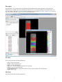
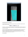
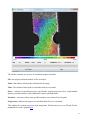
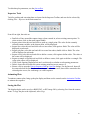
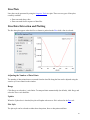
The user interface of Vic-2D has many of the familiar control elements found in other applications. The image below
illustrates the user interface. The most commonly used functions can be accessed by clicking on tool buttons on the Tool
Bar. The windows, such as the AOI Editor and Plot windows are grouped inside a Workspace. The List View on the left
of the main window provides a quick overview of image and data files.
File Menu
The File Menu provides the following functions:
z
z
z
z
z
z
z
New - creates a new project
Open - open an existing project
Save - save the current project
Save As... - save the current project under a new file name
Mode - select a Vic-2D project type
Install module licenses - use this menu entry to activate software modules you have purchased
Quit - quit Vic-2D
Edit Menu
The Edit Menu provides the following functions:
1
z
z
z
z
z
z
z
z
z
Undo - undo the last editing operation in the reference image
Redo - redo the last editing operation in the reference image
Pan/Select - pan around in a zoomed-in image, or select an existing AOI
Line - create a Line AOI
Rectangle - create a Rectangle AOI
Polygon - create a Polygon AOI
Cut Region - cut a region from a polygon or rectangle AOI
Delete - removes the selected AOI
Initial Guess - show the Initial Guess Dialog to select an initial guess for the currently active AOI
Project Menu
The Project Menu provides the following functions:
z
z
z
z
z
z
z
Speckle images- adds speckle images to the project for analysis.
Speckle image folder- adds all speckle images from a given folder.
Speckle image list - adds speckle images from a text-based list.
Calibration images - adds calibration images to the project.
Data files - adds pre-existing output data files to the project
Analog data - adds analog data files from Vic-Snap
Video clip - adds generated AVI files
Calibration Menu
The Calibration Menu provides the following functions:
z
z
z
z
Calibrate scale - allows calibration for physical scale.
Distortion correction - allows correction for nonparametric distortions.
Clear distortion - clears calculated distortion map.
More - additional functions including Aspect Ratio selection
Data Menu
The Data Menu provides the following functions:
z
z
z
z
z
z
Start analysis - shows the Run dialog to begin analysis
Apply math operation - allows manipulation of output data
Export statistics - exports group statistics for output data
Postprocessing options - shows a submenu to choose from various postprocessing calculations
Export data - exports output data for use with external software
Extract grid data - extracts and outputs data on a regular pixel grid
Plot Menu
The Plot Menu provides the following functions:
z
z
New plot- adds a new plot window to the work space
Inspector- allows choice of various data inspection tools
Window Menu
The Window Menu provides the following functions:
z
z
Cascade - organizes all MDI windows in a cascade
Tile - tiles all MDI windows
Help Menu
The Help Menu provides the following functions:
2
z
z
User manual - show this manual.
About - show version information.
Main Toolbar
The buttons on the main toolbar control commonly used Vic-2D functions. From left to right:
z
z
z
z
z
z
z
z
z
z
New project
Open project
Save project
Add speckle images
Add calibration images
Start analysis
Calculate strain
Histogram control
Zoom in/out
Undo/redo
The histogram control displays the gray level distribution for the currently displayed image. The red bars on the histogram
may be used to adjust the image display. Double-click on the histogram to automatically adjust the balance, or drag the red
bars to set the black and white levels manually. Double click again to remove the balance adjustment.
The balance control is for display only and does not affect image analysis or stored images.
Animation Toolbar
The buttons on the animation toolbar allow stepping through and animating image files or plots. The controls, from left to
right:
z
z
z
z
z
Play - begins automatically stepping through images/plots.
Stop - stops the animation.
Step Back / Step Forward - goes to previous or next image/plot.
Loop - toggles between looping from last image to first, and bouncing from forward to backward animation.
Frame rate - selects the speed of the animation..
Other Functionality
In the right corner of the status bar at the bottom of the main window, the cursor position and image
grey value is displayed when the mouse is moved inside the reference image or a deformed image. When
mousing over contour plots, coordinates as well as the value of the current contour variable will be
displayed.. On the left side of the status bar, a short description of tool buttons and menu items is
displayed when the mouse moves over them.
In the list view on the left side of the main window, some functions can be activated by right-clicking.
Details can be found in the appropriate sections of this menu.
3
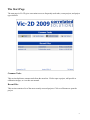
The Start Page
The start page in Vic-2D gives convenient access to frequently-used tasks, recent projects, and project
type selection.
Common Tasks
This section duplicates common tasks from the menu bar. Click to open a project, add speckle or
calibration images, or view this user manual.
Recent Files
This section contains a list of the most recently accessed projects. Click on a filename to open the
project.
4
Projects in Vic-2D
In Vic-2D, all the files and information associated with a test are stored in a project.
Initially, projects are blank. Before completing a Vic-2D analysis, the project must contain:
z
z
Two or more speckle images , including a reference image
One or more areas of interest
Note: Adding speckle and calibration images to the project adds them by filename reference only; they
are not copied or moved on the disk.
When you run a Vic-2D analysis, the output files are stored on a disk and added (by reference) to the
project file. If the project file is not saved or if the data files are manually removed, they will remain on
the disk.
In addition to the items above, you can also choose to add auxiliary data references to the project file:
z
z
Generated video clips
Analog data files from Vic-Snap
Notes
z
z
z
In general, it's good practice to save project files often to avoid losing changes.
Vic-2D 2009 uses a new .z2d project file format. Older .vic files may be opened, but not saved.
Once a calibration is performed and saved in the project file, the calibration images may be
discarded if desired. All the data calculated in the calibration routine is stored numerically in the
project file.
5
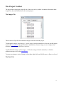
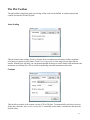
The Project Toolbar
The plot toolbar is displayed at the left side of the work area by default. It contains information about
image files, data, and calibration for the current project.
The Images Tab
This tab shows all speckle and calibration images associated with the project.
To add speckle images, select Images... Speckle images from the menu bar, or click the speckle images
icon on the main toolbar. The small red arrow indicates the reference image; to set an image as the
reference, right click and click Set as reference .
To add calibration images, select Images... Calibration images from the menu bar, or click the
calibration images icon on the main toolbar .
To remove an image or series of images, select them, right click, and click Remove or Remove selected .
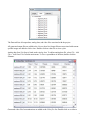
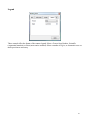
The Data Tab
6
The Data tab lists all output data, analog data, and video files associated with the project.
All generated output files are added to the Current data list. Output files not associated with current
speckle images are added to Other data. Double-click on a data file to view a plot.
Analog data from Vic-Snap is listed under Analog data. To add an analog data file, select File... Add
Files... Add Data Files from the main menu. To view a spreadsheet of the data, double-click the
filename.
Generated video files from animations are added to the Video files list. Double-click on a video to
7
display it in an external viewer.
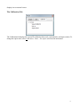
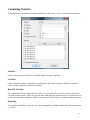
The Calibration Tab
The Calibration tab displays the current 2D calibration data (scale; selected units; and aspect ration). To
change the aspect ratio, select Calibration... More... Set aspect ratio from the main menu.
8
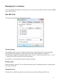
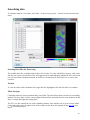
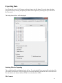
Speckle Images
In Vic-2D, speckle images are image or set of images taken of a specimen as it undergoes load or
motion. You may add one or multiple speckle images by selecting the Speckle images entry from the
Images menu, or by clicking the
icon on the main tool bar .
If more than 300-400 images are to be added, select Images... Speckle image folder to add all images
from a specified folder. Each valid image file from the selected folder will be added to the project;
extraneous / calibration images may then be removed. Trying to add too many images through the
Speckle images dialog may result in an error due to operating system limitations.
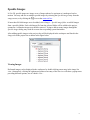
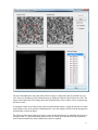
After adding speckle images to the project, they will be displayed in the workspace and listed in the
Images tab of the project bar as shown in the figure below.
Viewing Images
Deformed images can be displayed in the workspace by double-clicking on an entry in the image list
view. Alternatively, clicking the right mouse button on an entry of the list view will show a popup menu
providing different options, one of which is View .
9
When viewing deformed images, you can use the zoom in/zoom out entries in the Edit menu or the
corresponding tool buttons to change the scale of the displayed image.
Animating Images
To animate speckle images, display an image and then use the controls on the Animation Toolbar to
animate the sequence.
Removing Images
Calibration images can be removed by selecting one or multiple images in the list view, and rightclicking on your selection. Select Remove or Remove selected to remove images from the list.
10
The Reference Image
The term Reference Image is used in this manual to describe the image of the specimen taken while no
load was applied. All displacement analyses in Vic-2D are with respect to this reference image, i.e., the
displacements are obtained in a Lagrangian coordinate system.
To select a reference image, right-click on it in the Speckle images list, and select Set as reference.
After the reference image has been selected, it will be indicated with a red arrow in the images list.
When the reference image is displayed, the AOI tool buttons and menu entries in the Edit menu become
active.
11
Selecting an Area-of-Interest
Vic-3D supports the following types of AOIs:
z
z
z
Line: A number of points evenly spaced along a line. Note: data from line AOI's will not be
visible in 2D plots because it does not comprise an area. This data may be viewed in exported files
only.
Rectangle: Points spaced on an even grid contained in a rectangular area.
Polygon: Points spaced on an even grid contained in a polygon.
To specify a particular type of AOI, select the corresponding entry in the Edit menu or the appropriate
button on the tool bar. The selected AOI type will be indicated by the mouse cursor.
After selecting the AOI type, move the cursor to the desired position in the reference window and click
the left mouse button. You can now move the mouse to the next position, e.g. the end of the line or the
second corner of the rectangle. Clicking the left mouse button again will complete the AOI selection for
all AOI types except polygons. For polygon selection, a double-click is used to specify the last point of
the polygon.
During AOI selection, a yellow line is drawn to indicate the outline of the selection; small green squares
indicate nodes. This is illustrated in the figure below.
12
Choosing the Subset and Step Size
The subset and step size can be selected after an area of interest is created. Both are adjusted using the
spin boxes in the AOI Toolbar.
The subset size controls the area of the image that is used to track the displacement between images. The
subset size has to be large enough to ensure that there is a sufficiently distinctive pattern contained in the
area used for correlation.
The step size controls the spacing of the points that are analyzed during correlation. If a step size of 1 is
chosen, a correlation analysis is performed at every pixel inside the area-of-interest. A step size of 2
means that a correlation will be carried out at every other pixel in both the horizontal and vertical
direction, etc. Note that analysis time varies inversely with the square of the step size; i.e., a step size of
1 takes 25 times longer to analyze than a step size of 5.
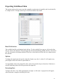
The Seed Point
13
The term Seed Point is used to refer to the point in the reference image where the correlation is started.
The correlation algorithms use the results from the seed point to obtain an initial guess for the second
point analyzed and continue in this manner until all points in the AOI are analyzed.
For rectangular and polygon AOIs, the seed point can be moved to a user-specified location in the AOI.
To move the seed point, select the 'Hand' tool, or select Edit... Pan/Select from the menu bar. Then,
mouse over the seed point; the cursor will change to indicate node movement. Click and drag to place
the seed point.
The placement of the seed point can greatly influence the amount of work required to select an initial
guess . Ideally, the seed point should be placed in the area of the image that underwent the smallest
amount of motion during the test. An example is illustrated in the figure below.
In this example, the seed point should be placed on the side of the image closest to the fixed grip of the
test frame, and on the center-line of the specimen. This way, even as the test progresses and the
specimen becomes more deformed, the start location for the correlation will experience relatively small
motions.
Editing AOIs
To edit an existing AOI, select the Pan/Select tool. Mouse over any of the green nodes in your AOI; the
mouse cursor changes to indicate node movement. Click and drag to move.
Cutouts
For rectangular and polygon AOIs, the scissors tool can be used to cut areas from the AOI. This feature
is most commonly used if the specimen has cracks, holes, or other areas where correlation is impossible.
14
To cut an area from an AOI, click the scissors button on the tool bar or select Edit... Cut region. The
selection of the area to be cut works like selecting a polygon AOI, i.e., corner points of a polygon can be
added by single-clicking the left mouse button, and the last point is specified by a double-click. Once the
cut is complete, new nodes are added to your AOI; these may be moved like other nodes.
Hints
z
z
z
z
Use the scroll wheel to adjust the size of the image.
When using multiple AOIs for one image, click on an AOI with the pan/select tool to activate it.
During AOI selection, the image can be scrolled by moving the mouse outside the reference image
window. This will cause the image to autoscroll if the image does not fit on the display.
You can use the Undo/Redo buttons to undo AOI selection and other operations. The Undo/Redo
buttons in the Edit menu will indicate what changes can be undone/redone.
15
Initial Guess Selection
In Vic-2D 2009, initial guesses will be needed very rarely. Some instances where they may still be necessary
include:
z
z
Very large motions between imags
Very fine or indistinct speckle patterns
In the absence of these conditions, you can generally run the correlation immediately after selecting an
AOI. If the correlation fails or runs very slowly, an initial guess may be needed.
Placing the seed point
Generally, it is best to place the seed point of the AOI in the area of the image that undergoes the least
amount of motion during the test. For instance, if a specimen is tested in a tensile frame, the seed point
should be placed as close to the stationary grip as possible. Placing the seed point this way will help
ensure fully automatic correlation.
For very large transformations or rotations, it can be very helpful to place fiducial marks on the surface.
This can be integrated into a printed pattern (see below) or simply drawn on the surface with a marker.
These marks may be located much more easily than the random pattern especially if, i.e., one image is
rotated 180 degrees from the other.
Selecting an initial guess
The initial guess dialog can be accessed through the Edit menu or the
The initial guess dialog is shown below.
tool button in the AOI toolbar.
16
The area surrounding the seed point in the reference image is displayed in the box labeled Reference
AOI. Next to it, the pattern in the deformed image is displayed in the box labeled Deformed AOI. The
image in the bottom left of the dialog shows the deformed image. Each of these can be zoomed using
the mouse wheel.
A histogram control is provided for the reference and deformed images. Adjust the red bars to control
image balance; this can be useful for finding detail in very dark images. Double click the histogram to
automatically set/reset the limits.
The listbox on the bottom right can be used to select the deformed image for which the initial guess is
being provided. If a green checkmark appears next to an image when activated, the initial guess has
been located automatically and no further intervention is required.
17
Selecting corresponding points
To select corresponding points in the reference and deformed image, the red cross in the bottom left
image has to be placed in the area of the deformed image that corresponds to the area around the seed
point in the reference image. This can be done by clicking and moving the mouse in the bottom image.
The scroll wheel can be used to zoom in and out; hold Shift and drag in the bottom image to pan. The
image in the Deformed AOI box is updated to reflect the location in the bottom image. Once the
Reference Aoi and Deformed Aoi images show the same region, common points can be selected.
Translation and Complete Guess
An initial guess can be specified for the translation components of the displacement only, or for the
complete deformation including the partial derivatives of the displacement. The latter will only be
neccessary in cases where the strains and/or rotations are very high.
Translation Guess
Follow the steps below to specify a translation guess:
{ Select a common point in the Reference Aoi and Deformed Aoi by clicking the mouse.
{ Click the Add Point button, or click the right mouse button. The point pair turns yellow, and a
guess is calculated. The icon in the file list will change to a green check to indicate that an initial
guess has been selected for the current image.
{ Optionally, repeat the first two steps for more corresponding points; the results will be an average
of all selected points. This can give higher accuracy but is usually not necessary.
{ If necessary, repeat this procedure for all deformed files shown in the file list.
Complete Guess
Follow the steps below to specify an initial guess that includes estimates for the partial derivatives of
the displacement (only necessary for very large strains and/or large rotations):
{ Check the Complete item in the Guess Type check box.
{ Select a common point in the Reference Aoi and Deformed Aoi by clicking the mouse.
{ Click the Add Point button or click the right mouse button.
{ Repeat for at least two more points. Note that the points should not be co-linear, i.e., try to select
three points that make a triangle.
{ Once at least three points are added, the icon in the file list will change to a green check to
indicate that an initial guess has been selected for the current image.
{ If necessary, repeat this procedure for all deformed files shown in the file list.
18
Running the Correlation
To run the displacement analysis, select the Run Correlation entry from the Data menu, or press the
button on the tool bar.
The File Tab
The tab on the dialog displays the following options:
Selecting Images
The deformed images to use for correlation analysis can be selected from the list box on the dialog.
Selected images are indicated by a check mark. Above the list box, buttons are available to
select/deselect all image files contained in the list box. To select 1 data file from from every 2, 5, 10, or
n , right-click in the file list and choose the desired option.
If no images are selected, only the reference image is analyzed.
Backup copies
When this option is checked, Vic-3D will make backup copies of existing output files by replacing their
file extension with bak.
Output directory
The directory in which the output files are stored can be selected by clicking the folder icon.
19
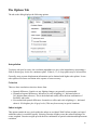
The Options Tab
The tab on the dialog displays the following options:
Interpolation
To achieve sub-pixel accuracy, the correlation algorithms use gray value interpolation, representing a
field of discrete gray levels as a continuous spline. Either 4-, 6-, or 8-tap splines may be selected here.
Generally, more accurate displacement information can be obtained with higher-order splines. Lowerorder splines offer faster correlation at the expense of some accuracy.
Criterion
There are three correlation-criteria to choose from:
z
z
z
Squared differences: Sensitive to any lighting changes; not generally recommended.
Normalized squared differences: Insensitive to scale in lighting (i.e., deformed subset is
50% brighter than reference.) This is the default and usually offers the best combination of
flexibility and results.
Zero-normalized squared differences: Insensitive to offset and scale in lighting (i.e., deformed
subset is 10% brighter plus 10 gray levels.) This may be necessary in special situations.
Subset weights
This option controls the way pixels within the subset are weighted. With Uniform weights, each pixel
within the subset is considered equally. Selecting Gaussian weights causes the subset matching to be
center-weighted. Gaussian weights provide the best combination of spatial resolution and displacement
resolution.
20
Exhaustive search
Enabling this option will cause Vic-2D to repeat a coarse search for matches after each time the
correlation fails. This may result in more data recovery at the expense of vastly increased processing
time.
Low-pass filter images
The low-pass filter removes some high-frequency information from the input images. This can reduce
aliasing effects in images where the speckle pattern is overly fine and cannot be well represented in the
image. (These aliasing effects are often visible as a moire-type pattern in the output data.)
Incremental correlation
With incremental correlation, each image is compared to the previous image rather than the reference
image. This can be useful in cases of pattern breakdown or extremely high strains (>100%). This comes
at the expense of an increase in noise.
Processor Optimizations
This option controls the number of processors/cores Vic-3D uses for analysis. In most cases this will be
correctly determined automatically by Vic-3D.
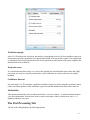
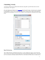
The Thresholding Tab
This tab provides options for removing any data that is bad or suspect while maximizing the amount of
retained data. Four thresholding options are available. For a typical test, the default values will work
very well, but when conditions are unusual or substandard (blur; debris; poor lighting; etc), some
adjustment may be required.
21
Prediction margin
After Vic-3D analyzes the seed point, the analysis is propagated to each of its four neighbors, and so on.
Each point is fed with a prediction of its approximate match. After the match is made, a back-prediction
is calculated. If the back-prediction does not closely match the actual location of the prior neighbor, this
threshold will remove the data.
Projection error
If a calculated match does not lie very close to the epipolar line, this threshold removes the data. High
projection error may be caused by motion blur; a poor calibration; or cameras which are not rigidly
mounted.
Confidence interval
For each match, Vic-3D calculates a statistical confidence region, in pixels, using the covariance matrix
of the correlation equation. If the confidence region exceeds this threshold, the data will be removed.
Matchability
This option automatically removes subsets that show a very low contrast, i.e, subsets that don't contain
very much information. Increase this value to remove more data; reduce to retain more data, i.e., if
lighting conditions were poor.
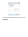
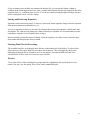
The Post-Processing Tab
The tab on the dialog displays the following options:
22
Strain Computation
Checking this option performs a strain computation as each image is processed; results can be viewed in
the preview.
Correlation Results
After you begin the correlation, the following window appears.
23
The window contains an overview of correlation progress and reults.
File - the progress and total number of files to analyze.
Points - the number of data points calculated for the image.
Time - The amount of time spent on correlation analysis in seconds.
Error - a measure of correlation accuracy (specificially, epipolar projection error). A high number
indicates possible problems with calibration or camera synchronization.
Iterations - a measure of how many possible matches were searched for each point.
Progress bar- indicates the progress of each individual file as it is correlated.
This window also contains a preview of the output data. This data may be view in 2D and 3D and
manipulated as with a standard plot.
24
When the analysis is complete, you may click View Report to see a summary of the above data.
For more information on interpreting correlation results and troubleshooting errors, please contact
Technical Support.
25
Smoothing data
To calculate strain for a set of data, select Data... Postprocessing options... Smooth variable from the main
menu.
Selecting Data Files for Processing
The available data files are displayed in the Data Files list box. To select which files to process, click on the
data file you want to select/deselect. This will toggle the check mark indicating whether the file is selected or
not. For convenience, the buttons labeled All and None select/deselect all files, while Invert reverses your
selection.
Preview
To view the effects of the calculation for a single data file, highlight the file and click the Preview button.
Filter size/type
Calculated strains are always smoothed using a local filter. The Method box allows selection of a smoothing
method. The decay filter is a 90% center-weighted Gaussian filter and works best for most situations; the box
filter is a simple unweighted averaging filter.
The Filter size box controls the size of the smoothing window. Since the filter size is given in terms of data
points rather than pixels, the physical size of the window on the object also depends on the step size used
during correlation analysis.
26
Strain Calculation
To calculate strain for a set of data, select Data... Postprocessing options... Calculate strain from the main menu.
Selecting Data Files for Processing
The available data files are displayed in the Data Files list box. To select which files to process, click on the data file
you want to select/deselect. This will toggle the check mark indicating whether the file is selected or not. For
convenience, the buttons labeled All and None select/deselect all files, while Invert reverses your selection.
Preview
To view the effects of the calculation for a single data file, highlight the file and click the Preview button.
Compute principal strains
Check this box to add principal strains and principal strain angle to the calculated output data.
Overwrite variables
Check this option to overwrite any existing strain calculations. If this box is clear, more data fields will be added to the
output data set each time strain is calculated.
Compute Tresca/von Mises strain
Select these options to compute the Tresca/von Mises strain criterion along with the strain tensor calculation.
Filter size/type
Calculated strains are always smoothed using a local filter. The Filter box allows selection of a smoothing method.
27
The decay filter is a 90% center-weighted Gaussian filter and works best for most situations; the box filter is a simple
unweighted averaging filter.
The Filter size box controls the size of the smoothing window. Since the filter size is given in terms of data points
rather than pixels, the physical size of the window on the object also depends on the step size used during correlation
analysis.
Tensor type
Select the desired strain tensor. The default is Lagrangian finite strain.
28
Rotation Calculation
To calculate local in-plane rotation for a set of data, select Data... Postprocessing options... Calculate
in-plane rotation from the main menu.
Selecting Data Files for Processing
The available data files are displayed in the Data Files list box. To select which files to process, click on
the data file you want to select/deselect. This will toggle the check mark indicating whether the file is
selected or not. For convenience, the buttons labeled All and None select/deselect all files, while Invert
reverses your selection.
Preview
To view the effects of the calculation for a single data file, highlight the file and click the Preview
button. You may view the plot in 2D or 3D as with a standard data plot.
Overwrite variables
Check this option to overwrite any existing rotation calculations. If this box is clear, more data fields
will be added to the output data set each time rotation is calculated.
Filter size/type
29
Calculated strains are always smoothed using a local filter. The Filter box allows
selection of a smoothing method. The decay filter is a 90% center-weighted Gaussian
filter and works best for most situations; the box filter is a simple unweighted
averaging filter.
The Filter size box controls the size of the smoothing window. Since the filter size is
given in terms of data points rather than pixels, the physical size of the window on the
object also depends on the step size used during correlation analysis.
30
Calculating Velocity
Vic-2D can calculate rates for displacement and strain, using either a specified time interval or time
retrieved from a .CSV log file.
Once the displacement fields have been calculated from the speckle images, velocities may be calculated
by selecting the Calculate Velocity entry on the Data menu. (If strain rates are desired, strain should be
calculated before opening the Calculate Velocity dialog.) This will display the dialog shown in the figure
below.
Data File Selection
The available data files are displayed in the list box. To select which files to process, click on the data
file you want to select/deselect. This will toggle the check mark indicating whether the file is selected or
not. For convenience, the buttons labeled All and None select/deselect all files; the Invert button inverts
31
the selection.
Velocity Calculation
If a Vic-Snap .CSV log file exists for the project, you may select "Time From File" from the dropdown
and select the file, if necessary. Otherwise, select "Constant Time Step" and enter the known time
increment, or select "Constant Frame Rate" to enter a known frame rate, for, i.e., a high-speed camera.
Click Start to begin; the progress bar will indicate completion. For each strain and displacement variable
in the dataset, a derivative in time will be added and can be viewed as a contour overlay.
32
Applying Functions to Data
Vic-3D supports the generation of new variables based on equations applied to the data. This feature can
be used, for instance, to compute engineering strains from Lagrange strains, to compute stresses from
strains or to compute thinning of a strained specimen of known thickness based on the Poisson's effect
or volume conservation during plastic deformation.
To apply function to a data sequence, select Data... Postprocessing options... Apply function from the
main menu.
Variable name and description
Enter a unique label for the variable name, e.g., sigma1 for the major stress, and an appropriate
description in the description field. Note that the description will be used in contour legends.
Equation
The formula to be applied to the data can be entered in the equation field. The equation is applied to
each data point contained in each data file. The variables present in the data file can be accessed in the
equation by their names. Not that variable names are case sensitive, e.g., X is the global coordinate and x
refers to the pixel coordinate. For a description of functions and operators that can be used in equations,
please see the equation format description.
33
If you are unsure what variables are contained in the data file, you can quickly obtain a listing of
variables in the following manner. First, enter a variable name known to be present in the data file in the
equation field, e.g., x and then press Preview. You can now obtain a listing by right-clicking in the plot
and accessing the Contour variables listing.
Storing and Retrieving Equations
Equations can be stored and reused. To retrieve a previously stored equation, simply select the equation
from the drop-down menu labeled Select eq..
To save an equation for later use, press the Save button after entering the equation, variable name and
description. The software will prompt for a label to identify the equation. It is recommended to test the
equation by using the Preview button before saving it.
Stored equations can also be removed. Simply select the equation you wish to remove from the dropdown menu and then press the Remove button.
Selecting Data Files for Processing
The available data files are displayed in the list box on the bottom left of the dialog. To select which
files to process, click on the data file you want to select/deselect. This will toggle the check mark
indicating whether the file is selected or not. For convenience, the buttons labeled All and None
select/deselect all files, while Invert reverses your selection.
Preview
To view the effects of the calculation for a single data file, highlight the file and click the Preview
button. You may view the plot in 2D or 3D as with a standard data plot.
34
Deleting Variables
User-generated variables can be deleted from data files. Note: Use this functionality with caution. Once
removed, variables cannot be restored other than by reprocessing.
To remove variables from data files, select Data... Postprocessing options... Map external data from the
main menu.
Selecting Data Files for Processing
The available data files are displayed in the list box on the left of the dialog. To select which files to
process, click on the data file you want to select/deselect. This will toggle the check mark indicating
whether the file is selected or not. For convenience, the buttons labeled All and None select/deselect all
files, while Invert reverses your selection.
Selecting Variables
The available variables are listed in the list box on the right of the dialog. Note that only user-generated
variables can be deleted. Select the variables you wish to remove by clicking on the variable name. This
will toggle a check mark indicating whether the variable will be removed or not.
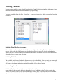
Rescanning Variables
If the data files do not all contain the same variables, the variable you are trying to remove may not
appear in the list box when the dialog is shown. In this case, highlight the data file that contains the
variable you wish to remove in the data file list box by clicking on it. Then, press the Rescan button to
repopulate the variable list box based on the variables contained in the selected data file.
35
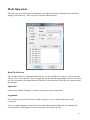
Math Operations
The Math operations dialog allows manipulation of output data by basic math operations. Open this
dialog by selecting Data... Math Operations from the main menu bar.
Data File Selection
The available data files are displayed in the list box. To select which files to process, click on the data
file you want to select/deselect. This will toggle the check mark indicating whether the file is selected or
not. For convenience, the buttons labeled All and None select/deselect all files; the Invert button inverts
the selection.
Operation
Choose Add, Subtract, Multiply, or Divide to perform the specified operation.
Arguments
The Variable box is used to select the variable to operate on. Any variable in the data set may
be selected.
To use a constant argument, select the Constant radio button and enter the value. For example, the
selections below will multiply the x-strain value from each data file by 100.
36
To use the data from an output file, click Data and select a data file. For example, the selections below
will subtract the first principal strain from the first data file, from all data files.
37
Click Start to begin; the progress bar will indicate completion. For each strain and displacement variable
in the dataset, a derivative in time will be added and can be viewed as a contour overlay.
38
Calculating Statistics
To export statistics for calculated variables and data files, select Data... Statistics from the main menu bar.
Statistics
Check the desired item to include or exclude the statistic from the output file.
Variables
Check the desired variables to add them to the calculation. By default, all metric variables are included,
while correlation and pixel variables are excluded.
Data File Selection
The available data files are displayed in the list box. To select which files to process, click on the data file
you want to select/deselect. This will toggle the check mark indicating whether the file is selected or not. For
convenience, the buttons labeled All and None select/deselect all files; the Invert button inverts the selection.
Exporting
To complete the calculation, click Ok. You will be prompted for a filename, and the data will be exported as
a .CSV file.
39
Exporting Data
For efficient file access, Vic-2D stores results in a binary data file format. To use the data with other
programs for post-processing and plotting, the data can be exported by selecting the Export item from
the Data menu.
The dialog shown below will be displayed.
Selecting Files for Exporting
The available data files are displayed in the list box. To select which files to export, click on the data file
you want to select/deselect. This will toggle the check mark indicating whether the file is selected or not.
For convenience, the buttons labeled All and None select/deselect all files.
File Formats
40
The data files can be exported to the following formats:
Comma-Separated Variable
Data entries are separated by commas. This format is understood by most spreadsheet
programs and plotting packages. Variable names are stored in the data file as commaseparated strings in quotation marks. Exported files will have the extension csv.
Tecplot
Used for plotting the data with Amtec's (www.amtec.com ) plotting program Tecplot(TM).
Exported files will have the extension dat.
Plain ASCII
This format is plain, space-delimited ASCII text data with one data point per line. Note:
There are no variable names in the data file, and data from different AOIs is concatenated.
Exported files will have the extension txt.
Matlab V4
This format provides compatibility with Matlab and many other programs capable of
reading Matlab files. Note that if multiple AOIs are present in a datafile, unique names for
each of the matrices are generated by appending increasing numbers to the variable names.
For instance, the X-coordinate for the first AOI will appear as X in the matlab file, and for
the second AOI it will appear as X_0 and so forth.
If none of the available file formats fit your needs, please contact [email protected]. We
will gladly implement data exporting to a format that best suits your needs.
41
Exporting Grid-Based Data
This option can be used to export your data, sampled at regular intervals spatially and for each data file,
to a single text file. To begin, select Export Grid Data from the Data menu.
Data File Selection
The available data files are displayed in the list box. To select which files to process, click on the data
file you want to select/deselect. This will toggle the check mark indicating whether the file is selected or
not. For convenience, the buttons labeled All and None select/deselect all files; the Invert button inverts
the selection.
Options
To change the sample interval in pixels, adjust the Sample step value. A value of 1 will sample every
pixel; higher values will result in a sparser data set.
To export blank values to the output file, with a value of 0, check the Export blanks box. If this box is
cleared, blank data points will not be present in the output file.
Extracting Data
To begin, click Start. You will be prompted for an output .csv file name. A progress bar will appear;
when extraction is complete, the dialog will close.
42
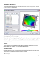
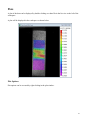
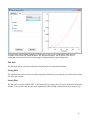
Plots
A plot of the data can be displayed by double-clicking on a data file in the list view to the left of the
workspace.
A plot will be displayed in the workspace as shown below.
Plot Options
Plot options can be accessed by right-clicking in the plot window.
43
The Contour variable submenu can be used to select the variable to display.
Click Show min. value or Show max. value to flag the location of the minimum or maximum value for
the currently selected variable.
Click Show reference data to view the data overlaid on the reference image rather than the deformed.
Click Change legend orientation to toggle between vertical and horizontal legend format.
Click Statistics to view a summary of data for the current image, for the currently selected contour
variable.
Click Change legend orientation to toggle between a horizontal and vertical legend.
Copy copies the current plot to the clipboard; Save allows saving the plot as an image file.
Select Export video to save an animated video.
Click Detach to keep this plot static instead of updating it each time a new data file is clicked in the Data
tab.
Editing Plot Parameters
44
To edit other plot parameters, use the plot toolbar.
Inspector Tools
Tools for probing and extracting data are located in the Inspector Toolbar, and can also be selected by
clicking Plot... Inspector in the main menu bar.
From left to right, the tools are:
z
z
z
z
z
z
z
z
z
Pan/Select: Pans around the contour image, when zoomed in; selects existing extract points. To
select an item, click on the small square handle.
Inspect point: select this tool and click to probe at a single point. The value for the currently
selected contour variable, at the chosen point, will be displayed.
Inspect line: select this tool and click once to start a line; click again to finish. The value will be
displayed at each node.
Inspect polyline: select this tool and click to create line nodes; double-click to finish. The value
will be displayed at each node.
Inspect circle: select this tool and click to define a center; click again to define a disc. The value at
the center will be displayed.
Inspect rectangle: select this tool and click to define a center; click again to define a rectangle. The
value at the center will be displayed.
COD (Crack Opening Displacement) tool: use this tool to calculate crack opening parameters.
Delete: choose this tool and click on an existing point/line/area to remove it.
Extract: click to open the Extract Sequence Data or Line Plot dialogs. For the line tool, data will
be extracted alone the line for the current image. For the other tools, data will be extracted at the
selected point or area, for each image, as a time sequence.
Animating Plots
To animate contour plots, bring up the plot display and then use the controls on the Animation Toolbar
to animate the sequence.
Saving the Plot
The displayed plot can be saved as a BMP, PNG, or JPG image file by selecting Save from the context
menu. To copy the plot to the clipboard, select Copy.
45
Output Variables
Introduction
During correlation and optional post-processing, Vic-3D presents a wide range of output data available for 3D
and contour plotting, extraction, and export.
Output Variables
Always Present
z
z
z
z
x / y [pixel] - point location in the reference speckle image
u / v [pixel] - pixel displacements
sigma [pixel] - this is the confidence interval for the match at this point, in pixels.
x / y / u / v [mm] - these are metric coordinates and displacements, when a calibration is present
Generated in Postprocessing
Strain Variables
z
z
z
z
z
z
exx [1] - strain in the X-direction. Positive numbers indicate tension; negative numbers indicate
compression.
eyy [1] - strain in the Y-direction.
exy [1] - shear strain.
e1 [1] - the major principal strain.
e2 [1] - the minor principal strain.
gamma [1] - the principal strain angle in radians, measure counterclockwise from the positive X-axis.
Velocity Variables
z
z
z
z
z
dU/dt [mm/s] - the rate of change of the U-displacement; that is, the velocity of a given point in the X
direction.
dV/dt [mm/s] - velocity in the Y direction.
dExx/dt [1/s] - the rate of change of strain in X, or strain rate in X.
dEyy/dt [1/s] - the strain rate in Y.
dExy/dt [1/s] - the shear strain rate.
Rotation Variables
z
phi [1] - the in-plane rotation, in radians.
Key Terms
Strain: the change in length, divided by initial length, for a solid material. For example, a strain of +10%
indicates that the material has expanded by 10%; a strain of -10% indicates that the material has contracted by
10%. Positive strains are referred to as tensile, while negative strains are compressive. Note: this is a finite
strain tensor and contains a quadratic term; for significant strains, this may result in a strain measure which is
larger than the small strain indicated by a strain gauge or extensometer.
Principal strain: the strain for a reference frame that is rotated such that shear becomes zero, leaving only two
strain components at 90� angles. The larger strain becomes the major principal strain, and the smaller
becomes the minor principal strain.
46
The Plot Toolbar
The plot toolbar is displayed at the top left edge of the work area by default. It contains options and
controls for both the 2D and 3D plots.
Auto-Scaling
This tab controls auto-scaling. Check or clear the boxes to enable auto-rescaling of either coordinate
axes limits, or contour overlay limits. Check Grow ranges only to allow ranges to get larger but not
smaller. With this box checked, you can animate through all images to set the limits to the minimum and
maximum over all data files. This is useful for producing consistent animations and videos.
Contour
This tab allows control of the contour overlay of 2D or 3D plots. To automatically scale these values to
fit the data, check the Auto-rescale contour box. To manually set the limits, clear this box and enter the
desired values.
47
To enable or disable the contour overlay in 3D mode, select Show contour plot.
Use the strain unit control to determine how strain values are displayed; the default is unity, i.e.,
mm/mm.
Color map
Use this tab to control the display of contour overlays. The Color map box chooses the overall color set
for the plot. The Opacity box sets the opacity of the overlay. The Levels box sets the n box sets the
number of discrete contour levels. The Level labels box controls the number of numeric level indicators.
Vector
This tab controls display of strain and displacement vectors.
Major and minor strain direction vectors are displayed when strain data is available Skip and scale
control the size and density of the vectors. The use solid color checkbox causes the vectors to be
displayed in a single color rather than the underlying plot color; the color selector button can be used to
choose this color.
48
Legend
These controls affect the format of the contour legend. Select a Format from Number, Scientific
(exponential notation), or Best (most concise method). Select a number of Digits, or Automatic to use as
much precision as necessary.
49
Exporting Videos
To export an animation from a plot, right-click in the plot and select Export Video.
If the auto-rescaling feature is enabled for contours, you will see a warning:
When rescaling is on, the animation may not appear as expected because each frame will be scaled
differently. Click Yes to continue or Cancel to correct the condition. When complete, the following
dialog appears:
File
Click the icon to select a filename for saving.
Encoder
To export a video file, select AVI from the Encoder drop-down; to export individual frames as separate,
numbered files, select Image Sequence.
50
Format
Select from available compression formats; options will vary based on system configuration and
installed codecs. Indeo(R) Video 5.11 works well for most Windows XP systems. RGB Uncompressed
videos will be high quality but very large.
Frame rate
Select a frame rate in frames per second for the video.
Data File Selection
The available data files are displayed in the list box. To select which files to process, click on the data
file you want to select/deselect. This will toggle the check mark indicating whether the file is selected or
not. For convenience, the buttons labeled All and None select/deselect all files; the Invert button inverts
the selection.
To begin, click Export; a progress bar will indicate completion.
51
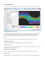
Line Plots
Line plots can be generated by using the Inspector Tools in a plot. There are two types of line plots
currently available:
z
z
Data extracted along a line
Data extracted from a sequence of data files
Line Data Extraction and Plotting
The line data plot appears when the Extract button is pushed on the Plot while a line is selected:
Adjusting the Number of Data Points
The number of data points that are extracted from the data file along the line can be adjusted using the
Number of Points control on the window.
Range
Click Range to select the x/y axis limits. To compute limits automatically (the default), click Range and
select the Auto-scale checkbox.
Update
When the Update box is checked, the plot will update when a new file is selected in the Data tab..
Plot Style
The plot style can be selected to either show data points, lines or data points and lines.
52
Save Data
Click to save data from one or several extractions. The following dialog will appear:
Select the variables to extract and the files to include in the extraction. The data may be organized by
columns or rows; to include a row/column header which contains the name of the relevant data file, select
Write header.
Saving Plots
The plot can be saved as a BMP, PNG, or JPG image file by pressing Save Plot in the bottom left of the plot
window. You may also copy the plot to the clipboard by right-clicking on the plot area and selecting Copy.
Sequence Data Extraction and Plotting
The sequence data extraction window appears when the Extract button is pushed on the 2D Plot while a
point, circle, or rectangle is selected:
53
Selecting Data Files
The data files used for extraction can be selected in the listbox in the top left of the window on the Extract
tab.
Selecting Variables
The variables to extract from the files can be selected in the listbox in the bottom left of the window on the
Extract tab.
If an analog data file is present, time and analog data values may be selected for either axis.
Extracting the Data
After selecting the data files and variables to extract, push the Extract button to extract the data. Depending
on the size and number of data files, this might take some time and a progress indicator will be shown to
indicate the extraction progress. After data extraction, the Plot tab will become active and the window will
appear as follows:
54
You can select from available variables for both X and Y axes. For an extensometer extraction, the
available values will be D0 (initial distance), D1 (deformed distance), and E (strain). This is not a
Lagrangian strain but only the first order change in length divided by initial length term.
Plot Style
The plot style can be selected to either show data points, lines or data points and lines.
Saving Data
The extracted data can be saved as a comma-separated variable file by pressing the Save Data in the bottom
left of the plot window.
Saving Plots
The plot can be saved as a BMP, PNG, or JPG image file by pressing Save Plot in the bottom left of the plot
window. You may also copy the plot to the clipboard by right-clicking on the plot area and selecting Copy.
55
Quick Start
There are only a few steps involved in obtaining deformation measurements from your images. If you
are using Vic-2D for the first time, take a look at the example provided with the program. Then, try to
go through the following steps yourself to quickly familiarize yourself with the program usage:
1.
Add a reference image and select your area of interest.
2.
Add more speckle images.
3.
Run the correlation analysis.
4. Plot the results
If you encounter any difficulties, please do not hesitate to contact our technical support department .
56
What's New in Vic-2D 2009
z
z
z
z
z
z
z
z
z
z
New matching algorithm for improved accuracy.
Multi-core parallel processing for major speed increase on modern PC's.
Confidence interval reporting on displacement data.
More flexible AOI selection.
Improved plotting and extraction tools.
New thresholding options for accurate rejection of incorrect data with minimal loss.
Arbitrary math functions can be created, saved, and applied to data; compute resultants, custom
strain tensor values, and more.
Improvements in data export including new Matlab format.
Improved strain calculation accuracy and more flexible options.
Incremental correlation option tracks strains to 1,000% and above.
57
Technical Support
If you cannot find an answer to your question in this manual, please do not hesitate to contact our
technical support at [email protected]. You can also find contact information at our web
site at www.correlatedsolutions.com.
We will be happy to assist with topics such as:
z
z
z
z
Designing digital image correlation experiments
Troubleshooting errors
Interpreting test data
Achieving optimal results
Bug Reports and Feature Requests
If you encounter a bug in Vic-2D, please let us know about it. Send a short description of the problem to
[email protected], along with any project or image files you think may help us
reproduce the bug.
Also, if you think Vic-3D can be improved by adding a particular feature you would find helpful, let us
know about it. We will try to incorporate your requests in our future updates of the software.
58