1
ADAS809: Non-Maxwellian modelling - change
adf04 file type
The program converts an ADF04 – type 1 file to a standard ADF04 – type 3 file. That is an ADF04 file
with collision strength data is converted to an ADF04 file with Maxwell averaged collision strengths.
Background theory:
The tabulation of the electron impact excitation and ionisation data in an ADF04 – type 1 file is of
collision strength Ω versus threshold parameter X . X = ε i / ∆E ij where ∆E ij is the energy of the
transition i → j and ε i is the incident electron energy with the target in the lower energy state i . At
the finest energy resolution, collision strengths display detailed resonance structure. It is assumed that
the tabulated collisions strengths in the ADF04 – type 1 file are smoothly varying, that is they have
been subject to some averaging over resonant structure. It is evident that if the ‘width’ of the averaging
interval above is ∆E res − avge , then the generation of Maxwell averaged collision strengths at
temperature Te is meaningful only if kTe >> ∆E res − avge . The numerical quadrature procedure takes
account of dipole, non-dipole and spin change forms for excitation. The behaviours for transition
i → j are as
Ωij ≈ F3 Sij log( X + F2 )
dipole:
non − dipole: Ω ij ≈ F3 + F2 X
9.9.1
spin change: Ω ij ≈ F3 ( X + F2 ) 2
where F2 and F3 are constants. In the dipole case, asymptotically F3 = 4 3 . Sij is the line strength for
the transition. For ionisation, the dipole form with F3 S ij replaced by the single constant F3 ' is
appropriate. For electron impact excitation of ions, the collision strength tends to a finite value at
threshold. In contrast, for neutral atom excitation and ionisation, the collision strength tends to zero at
α
theshold, with the threshold behaviour Ω ~ aX . Usually
α ~ 1 for ionisation of both atoms and ions.
α = 1 / 2 for neutral atom excitation and
For the tabulation {( X k , Ω k ) : k = 1,...,n } , the quadrature
∞
Υij = ∫ Ω ij (ε j ) exp( − ε j kTe ) d (ε j kTe )
9.9.2
0
is expressed as
Υij = ( ∆Eij kTe ) exp( ∆Eij kTe )
∞
∫Ω
ij
9.9.2
( X ) exp[ − X ( ∆Eij kTe ))] dX
1
∫
,
∫
X1
1
∞
Xn
X1
and the integral divided into the ranges
and
∫
. The asymptotic behaviours extrapolating
Xn
from the first and last two tabular points are used in the evaluation of the first and last integrals
respectively. The second integral is evaluated piece-wise in each tabular interval with the integrand
locally fitted to a quadratic in either a linear scale (ie. Ω = c1 + c 2 X + c3 X ) or logarithmic scale
2
picture (ie. lnΩ = c1 + c 2 ln X + c3 lnX ).
Quadrature precision is checked from the exact integrals of the approximate forms, namely,
2
ADAS User manual
Chap9-09
17 March 2003
dipole :
Υij ≈ F3 S ij [ln( 1 + F2 ) + EEI (( 1 + F2 )∆Eij / kTe )]
non − dipole : Υij ≈ F3 + F2 ( ∆Eij / kTe )EEI ( ∆Eij / kTe )
spin change : Υij ≈
F3 ( ∆Eij / kTe )
1 + F2
9.
EE 2(( 1 + F2 )∆Eij / kTe )
9.3
where EEI ( x ) = exp( x ) E1 ( x ) and EE 2( x ) = exp( x ) E 2 ( x ) with E 1 and E 2 the first and
second exponential integrals. A further verification on the quadratures is from the exact integrals for
Ω = constant, Ω = X − 1 and Ω = ( X − 1)2 which are exact for the quadratic fit, linear scale
option.
The program has a capability for comparison and display. In addition to the input ADF04 – type 1 file
for conversion, it can accept a second ADF04 – type 3 file. The temperature set for output is copied
from the latter reference file. Additionally, the collision data for a selected single transition may be
graphed along with the corresponding data from the reference file if it exists. The usual display and
output routing facilities are provided.
Program steps:
These are summarised in figure 8.9.
Figure 8.9
!
VHOHFW VSHFLILF
LRQ ILOH
HQWHU ILW FKRLFHV
UHDG DQG YHULI\
!
!
VSHFLILF LRQ ILOH
VHOHFW WUDQVLWLRQ
DQG RXWSXW
EHJLQ
WHPSHUDWXUHV
UHSHDW
UHSHDW
FRPSXWH FXELF
!
VSOLQH DQG
!
PLQLPD[ ILW
GLVSOD\ H[FLW
2XWSXW WDEOHV
DQG JUDSKV
HQG
UDWH FRHIIW
JUDSK
Interactive parameter comments:
Remember to ensure you have a defaults directory allocated. This should have the pathway
/..../uid/adas/defaults
where uid is your user identifier. The defaults directory records the parameters you set the last time
you ran each ADAS code. Move to the directory in which you wish any ADAS created files to appear.
These include the output text file produced after executing any ADAS program (paper.txt is the
default) and the graphic file if saved (e.g. graph.ps if a postscript file). Initiate ADAS, move to the
series 2 menu and click on the first button to activate ADAS201.
The file selection window has the appearance shown below
1. Selection of two adf04 files is permitted. The first selected in the upper
sub-window is of adf04 – type1 and is mandatory. The second optional
file, selected in the lower sub-window is of adf04-type3. It provides a
temperature grid for the conversion. Selection of the adf04 files follows
the standard ADAS.
2. Data root shows the full pathway to the appropriate adf04 data
subdirectories. Click the Central Data button to insert the default central
ADAS pathway to the correct data type. Click the User Data button to
insert the pathway to your own data. Note that your data must be held in
a similar file structure to central ADAS, but with your identifier
ADAS User manual
Chap9-09
17 March 2003
replacing the first adas, to use this facility. The Data root can be edited
directly. Click the Edit Path Name button first to permit editing.
3. Available sub-directories are shown in the large file display window.
Scroll bars appear if the number of entries exceed the file display
window size. Click on a name to select it. The selected name appears in
the smaller selection window above the file display window. Then its
sub-directories in turn are displayed in the file display window.
Ultimately the individual datafiles are presented for selection. Datafiles
all have the termination .dat.
2
3
1
4
4. Once the adf04 files are selected, the set of buttons at the bottom of the
main window become active. Clicking on the Browse Comments button
displays the comment line information stored with the adf04 datafile. It
ADAS User manual
Chap9-09
17 March 2003
is important to use this facility to find out what is broadly available in
the dataset. The possibility of browsing the comments appears in the
subsequent main window also.
The processing options window has the appearance shown below:
1. An arbitrary title may be given for the case being processed. For
information the full pathway to the dataset being analysed is also shown.
The button Browse comments again allows display of the information field
section at the foot of the selected dataset, if it exists. A summary of the
number of electronic transitions and energy levels is also given.
1
3
2
4
.
2
2.
ADAS User manual
Transitions for which electron impact excitation data are available in the
data set are displayed in the line list display window. This is a scrollable
window using the scroll bar to the right of the window. Click anywhere on
Chap9-09
17 March 2003
3.
4.
5.
the row for a line to select it. The selected transition appears in the selection
window just above the line list display window. This single transition will
displayed.
The output rate coefficient for the selected transition may be fitted with a
polynomial. This is as a function of temperature. Clicking the Fit
Polynomial button activates this. The accuracy of the fitting required may
be specified in the editable box. The value in the box is editable only if the
Fit Polynomial button is active.
To obtain an output adf04-type3 file output temperatures must be selected.
If a comparative adf04-type3 file was selected, the Input temperatures are
taken from that file. Otherwise temperatures from the Defaults file are used.
Pressing the Default Temperature values button inserts a default set of
temperatures equal to the input temperatures
The Temperature Values are editable. Click on the Edit Table button if you
wish to change the values. A ‘drop-down’ window, the ADAS Table Editor
window: It follows the same pattern of operation as described in bulletin.
The output options window is as shown below
1. As in the previous window, the full pathway to the file being analysed is
shown for information. Also the Browse comments button is available.
1
2
3
.
2
ADAS User manual
Chap9-09
17 March 2003
2.
3.
4.
Graphical display is activated by the Graphical Output button. This will
cause a graph to be displayed following completion of this window. When
graphical display is active, an arbitrary title may be entered which appears
on the top line of the displayed graph. By default, graph scaling is adjusted
to match the required outputs. Press the Explicit Scaling button to allow
explicit minima and maxima for the graph axes to be inserted. Activating
this button makes the minimum and maximum boxes editable.
Hard copy is activated by the Enable Hard Copy button. The File name box
then becomes editable. If the output graphic file already exits and the
Replace button has not been activated, a ‘pop-up’ window issues a warning.
A choice of output graph plotting devices is given in the Device list
window. Clicking on the required device selects it. It appears in the
selection window above the Device list window.
The Text Output button activates writing to a text output file. The file name
may be entered in the editable File name box when Text Output is on. The
default file name ‘paper.txt’ may be set by pressing the button Default file
name. A ‘pop-up’ window issues a warning if the file already exists and the
Replace button has not been activated.
The graph is displayed in a following Graphical Output window.
ADAS User manual
Chap9-09
17 March 2003