Download User`s manual

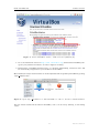
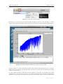
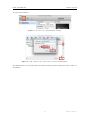
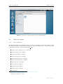
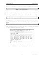
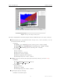
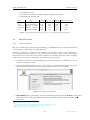
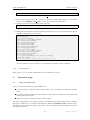
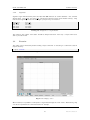
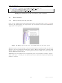
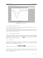
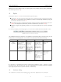
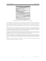
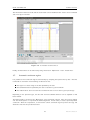
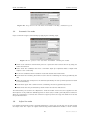
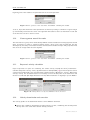
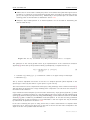
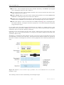
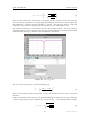
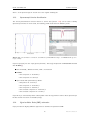
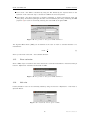
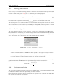
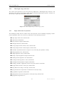
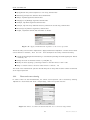
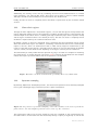
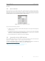
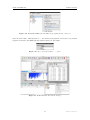
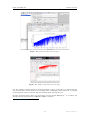
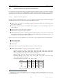
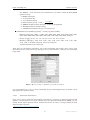
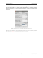
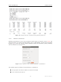
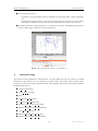
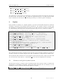
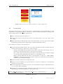
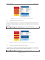
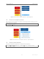
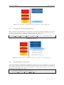
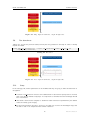
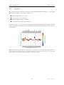
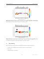
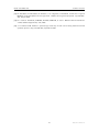
iSpec: Integrated Spectroscopic Framework
User’s manual
DR
AF
T
Author:
Sergi Blanco-Cuaresma
July 28, 2015
iSpec framework
User’s manual
Contents
1 Introduction
3
2 Installation
3
2.1
Virtual Machine . . . . . . . . . . . . . . . . . . . . . . . . . . . . . . . . . . . . . .
3
2.2
GNU/Linux systems . . . . . . . . . . . . . . . . . . . . . . . . . . . . . . . . . . . .
7
2.2.1
Python distribution . . . . . . . . . . . . . . . . . . . . . . . . . . . . . . . .
7
2.2.2
iSpec Framework . . . . . . . . . . . . . . . . . . . . . . . . . . . . . . . . .
8
MacOSX systems . . . . . . . . . . . . . . . . . . . . . . . . . . . . . . . . . . . . .
10
2.3.1
Python distribution . . . . . . . . . . . . . . . . . . . . . . . . . . . . . . . .
10
2.3.2
iSpec framework . . . . . . . . . . . . . . . . . . . . . . . . . . . . . . . . . .
11
2.3
3 Interactive usage
3.1
11
Input and output files . . . . . . . . . . . . . . . . . . . . . . . . . . . . . . . . . . .
11
3.1.1
Spectra . . . . . . . . . . . . . . . . . . . . . . . . . . . . . . . . . . . . . .
12
3.1.2
Continuum . . . . . . . . . . . . . . . . . . . . . . . . . . . . . . . . . . . . .
12
3.1.3
Lines . . . . . . . . . . . . . . . . . . . . . . . . . . . . . . . . . . . . . . . .
12
3.1.4
Segments . . . . . . . . . . . . . . . . . . . . . . . . . . . . . . . . . . . . .
13
3.2
Execution . . . . . . . . . . . . . . . . . . . . . . . . . . . . . . . . . . . . . . . . .
13
3.3
Basic interaction . . . . . . . . . . . . . . . . . . . . . . . . . . . . . . . . . . . . . .
14
3.3.1
Opening, selecting and closing spectra files . . . . . . . . . . . . . . . . . . .
14
3.3.2
Opening and closing region files . . . . . . . . . . . . . . . . . . . . . . . . .
15
3.3.3
Saving images, spectra and regions . . . . . . . . . . . . . . . . . . . . . . . .
15
3.3.4
Visualization . . . . . . . . . . . . . . . . . . . . . . . . . . . . . . . . . . . .
15
3.4
Regions . . . . . . . . . . . . . . . . . . . . . . . . . . . . . . . . . . . . . . . . . .
16
3.5
Continuum fitting . . . . . . . . . . . . . . . . . . . . . . . . . . . . . . . . . . . . .
16
3.6
Line fitting . . . . . . . . . . . . . . . . . . . . . . . . . . . . . . . . . . . . . . . . .
18
3.7
Automatic continuum regions . . . . . . . . . . . . . . . . . . . . . . . . . . . . . . .
19
3.8
Automatic line masks . . . . . . . . . . . . . . . . . . . . . . . . . . . . . . . . . . .
20
3.9
Adjust line masks . . . . . . . . . . . . . . . . . . . . . . . . . . . . . . . . . . . . .
20
3.10 Create segments around line masks . . . . . . . . . . . . . . . . . . . . . . . . . . . .
21
3.11 Barycentric velocity calculation . . . . . . . . . . . . . . . . . . . . . . . . . . . . . .
21
3.12 Velocity determination and correction . . . . . . . . . . . . . . . . . . . . . . . . . .
21
3.13 Spectroscopic binaries identification . . . . . . . . . . . . . . . . . . . . . . . . . . .
25
3.14 Signal-to-Noise Ratio (SNR) estimation . . . . . . . . . . . . . . . . . . . . . . . . .
25
3.15 Errors estimation . . . . . . . . . . . . . . . . . . . . . . . . . . . . . . . . . . . . .
26
1
Draft version
3.16 Add noise . . . . . . . . . . . . . . . . . . . . . . . . . . . . . . . . . . . . . . . . .
26
3.17 Resolving power estimation . . . . . . . . . . . . . . . . . . . . . . . . . . . . . . . .
27
3.18 Resolution degradation . . . . . . . . . . . . . . . . . . . . . . . . . . . . . . . . . .
27
3.19 Continuum normalization . . . . . . . . . . . . . . . . . . . . . . . . . . . . . . . . .
27
3.20 Wavelength range reduction . . . . . . . . . . . . . . . . . . . . . . . . . . . . . . . .
28
3.21 Apply mathematical expression . . . . . . . . . . . . . . . . . . . . . . . . . . . . . .
28
3.22 Fluxes and errors cleaning . . . . . . . . . . . . . . . . . . . . . . . . . . . . . . . . .
29
3.23 Clean telluric regions . . . . . . . . . . . . . . . . . . . . . . . . . . . . . . . . . . .
30
3.24 Spectrum resampling . . . . . . . . . . . . . . . . . . . . . . . . . . . . . . . . . . .
30
3.25 Spectra combination . . . . . . . . . . . . . . . . . . . . . . . . . . . . . . . . . . . .
31
3.26 Interoperability with other SAMP applications . . . . . . . . . . . . . . . . . . . . . .
31
3.27 Spectral synthesis and parameter determination . . . . . . . . . . . . . . . . . . . . .
34
3.27.1 Synthetic spectrum generation . . . . . . . . . . . . . . . . . . . . . . . . . .
34
3.27.2 Parameters determination . . . . . . . . . . . . . . . . . . . . . . . . . . . . .
35
3.27.3 Abundance determination . . . . . . . . . . . . . . . . . . . . . . . . . . . . .
37
4 Automatic usage
38
5 Pipeline
40
5.1
Generate a small grid of synthetic spectra . . . . . . . . . . . . . . . . . . . . . . . .
40
5.2
Pre-processing . . . . . . . . . . . . . . . . . . . . . . . . . . . . . . . . . . . . . . .
41
5.3
Generate list of pre-processed spectra
. . . . . . . . . . . . . . . . . . . . . . . . . .
42
5.4
Determine atmospheric parameters and normalize . . . . . . . . . . . . . . . . . . . .
42
5.5
Generate list of atmospheric parameters . . . . . . . . . . . . . . . . . . . . . . . . .
43
5.6
Determine chemical abundances . . . . . . . . . . . . . . . . . . . . . . . . . . . . .
43
5.7
Generate list of chemical abundances . . . . . . . . . . . . . . . . . . . . . . . . . . .
44
5.8
Flag abundances to be filtered . . . . . . . . . . . . . . . . . . . . . . . . . . . . . .
44
5.9
Plot abundances . . . . . . . . . . . . . . . . . . . . . . . . . . . . . . . . . . . . . .
45
5.10 Setup . . . . . . . . . . . . . . . . . . . . . . . . . . . . . . . . . . . . . . . . . . . .
45
5.11 Visualizing the results . . . . . . . . . . . . . . . . . . . . . . . . . . . . . . . . . . .
46
5.12 Assessment
47
6 Bug reporting
. . . . . . . . . . . . . . . . . . . . . . . . . . . . . . . . . . . . . . . .
48
iSpec framework
1.
User’s manual
Introduction
iSpec is an open source framework for spectral analysis [1]. It is suitable for the creation of spectral
libraries such as the Gaia FGK Benchmark Stars library [2] and the determination of astrophysical
parameters such as effective temperature, surface gravity, metallicity and individual abundances. iSpec
works in conjunction with “SPECTRUM: a Stellar Spectral Synthesis Program” [3] for the generation
of synthetic spectra and the derivation of abundances from equivalent widths.
The framework can be used from python scripts in an automatic way by using its API, but it also includes
a visual interface that is SAMP ready and it can interoperate with other astronomical applications such
as TOPCAT1 , VOSpec2 and splat3 facilitating a indirect way to access the Virtual Observatory4 .
iSpec can be downloaded from http://www.blancocuaresma.com/s/. It is distributed under the
terms of the GNU Affero General Public License5 (open source license), except the SPECTRUM code
which is also included in the framework thanks to R. O. Gray. The latest SPECTRUM version can also
be obtained from http://www.appstate.edu/~grayro/spectrum/spectrum.html.
This document presents the installation steps for the iSpec framework, together with a general overview
of the functionalities that can be accessed through the visual interface and from python scripts.
2.
Installation
2.1.
Virtual Machine
The fastest way to experiment with iSpec on any platform (Mac, Windows, Linux and Solaris) is to use
a ready-to-use the virtual machine with iSpec and all its dependencies already included (i.e. python
packages and compilers). To run it, the only necessary step is to install the sofware for running virtual
machines called VirtualBox (free software):
1 http://www.star.bris.ac.uk/
~mbt/topcat/
2 http://www.sciops.esa.int/index.php?project=ESAVO&page=vospec
3 http://star-www.dur.ac.uk/
4 http://www.ivoa.net/
~pdraper/splat/splat.html
5 https://www.gnu.org/licenses/agpl-3.0.html
3
Draft version
iSpec framework
User’s manual
Figure 1: Oracle VirtualBox website, download section (2014/03/31).
1. Go to the ”Download” section of http://www.virtualbox.org, download the VirtualBox package for your platform and install it. A reboot might be necessary.
2. Download the ”VirtualBox Extension Pack” too (platform independent), executed it and it will
be automatically integrated into your installation of VirtualBox.
Once installed, the iSpec virtual machine can be decompressed and recognized by VirtualBox by opening
“iSpec Xubuntu.vbox”:
Figure 2: Open “iSpec Xubuntu.vbox” with VirtualBox to add it to the list of virtual machines.
The new virtual machine will be listed in VirtualBox, now it can be run by selecting it and clicking
“Start”:
4
Draft version
iSpec framework
User’s manual
Figure 3: Start the virtual machine.
By default, the virtual machine will show the Xubuntu Desktop with two icons that allow to execute
iSpec (normal execution and test). Double clicking the test will launch iSpec with the example spectra:
Figure 4: Virtual machine running iSpec with a solar spectrum.
iSpec is installed on “/home/virtual/shared/iSpec” in the virtual machine (check section 2.2.2 for more
details about the contents) and the application can also be executed from the terminal by invoking
“ispec” in any directory.
It is also possible to share a folder from your real computer to the virtual one, thus files can be easily
accessed from it. To activate that option, go to “Settings - Shared folders” and add a shared folder by
clicking on the plus sign. It is important to mark the “Auto-mount” option to have an easier access
5
Draft version
iSpec framework
User’s manual
from the virtual machine:
Figure 5: Access to the virtual machine settings.
Figure 6: Add a shared folder between the real and virtual machine.
The shared folder can be accessed from the virtual machine by double clicking the folder “media” on
the Desktop:
6
Draft version
iSpec framework
User’s manual
Figure 7: Access to a shared folder from the virtual machine.
2.2.
GNU/Linux systems
2.2.1.
Python distribution
On debian based GNU/Linux distributions such as Ubuntu or Linux Mint, the following packages should
be installed by using the visual package manager (i.e. Ubuntu Software Center6 or Synaptic7 ) or from
a terminal by executing “apt-get install package name”8 :
ˆ python (2.7.5 or higher but not 3.x branch)
ˆ python-numpy (1.9.2 or higher)
ˆ python-scipy (0.16.0 or higher)
ˆ python-astropy (1.0.3 or higher)
ˆ python-matplotlib (1.4.3 or higher)
ˆ python-statsmodel (0.6.1 or higher)
ˆ python-pip (1.5.4 or higher)
ˆ cython (0.22.1 or higher)
ˆ gfortran (4.8.4 or higher)
ˆ lockfile (0.10.2 or higher)
ˆ build-essential
6 http://www.ubuntu.com/ubuntu/features/ubuntu-software-centre
7 http://wiki.debian.org/Synaptic
8 Administrator
rights will be needed.
7
Draft version
iSpec framework
User’s manual
Optionally, one extra package can be installed by using the python package installer PIP from a terminal
(only needed if we want iSpec to comunicate with TOPCAT or similars):
1
pip
i n s t a l l sampy
Listing 1: Extra packages installation
2.2.2.
iSpec Framework
Once the system is ready for execution of python applications, it is possible to proceed with iSpec
installation by decompressing the editor’s file “iSpec v20150728.tar.gz” (the version number may vary
with time):
1
2
t a r −z x v f i S p e c v 2 0 1 5 0 7 2 8 . t a r . gz
cd i S p e c v 2 0 1 5 0 7 2 8
Listing 2: iSpec installation
[OPTIONAL] In case we want to have the functionality of generating synthetic spectrum and determining astrophysical parameters, an additional step should be executed in order to compile the needed
libraries:
1
make
Listing 3: Compilation of “SPECTRUM: a Stellar Spectral Synthesis Program” [3]
Finally, it is possible to test iSpec by double clicking “test.command” (or executing “./test.command”
in a terminal) and selecting a star by entering its number:
Figure 8: Test execution script which allows to view 5 different stars.
8
Draft version
iSpec framework
User’s manual
Figure 9: iSpec showing several spectra.
The iSpec compressed file contains the program and some additional data in the “input/” directory:
ˆ Observed spectra for 5 very well-known stars: Procyon, Sun, µ Cas A, Arcturus, µ Leo (input/spectra/example/ directory)
– Filenames:
* NARVAL *.s.gz: NARVAL[4] spectra (resolving power ∼70,000 - 90,000)
* ESPaDOnS *.s.gz: ESPaDOnS[5]spectra (resolving power ∼68,000 - 81,000)
* HARPS *.s.gz: HARPS[6] spectra (resolving power ∼115,000)
– Characteristics:
*
*
*
*
*
Not normalized
Radial velocity not corrected
Barycentric correction applied
Resolution depends on the instrument
Wavelength range from ∼480 to ∼680 nm
ˆ ELODIE[7] spectra for binarity tests (input/spectra/binaries/ directory, see section 3.12):
– Filenames:
* elodie hd005516A spectroscopic binary.s.gz
* elodie hd085503 single star.s.gz
– Characteristics:
* Not normalized
* Resolution ∼42,000
* Wavelength range from ∼400 to ∼680 nm
ˆ Regions (input/regions/ directory):
– Example of continuum regions
9
Draft version
iSpec framework
User’s manual
– Line masks for Fe I/II
– Line masks for the wings of H-Alpha, H-Beta and Magnesium triplet.
– Segments for the previous lines
Star
Procyon
Sun
µ Cas A
Arcturus
µ Leo
Type
Teff (K)
Log g (dex)
[M/H]
Radial Vel. (km/s)
Metal Rich Dwarf
Metal Rich Dwarf
Metal Poor Dwarf
Metal Poor Giant
Metal Rich Giant
6545
5777
5308
4247
4433
3.99
4.44
4.41
1.59
2.50
-0.02
0.00
-0.89
-0.54
0.29
-3.2
0.00
-96.06
-5.18
14.25
Table 1: Astrophysical paramters for the 5 very well-known stars included
2.3.
MacOSX systems
2.3.1.
Python distribution
One of the easiest ways to install a Python distribution on MacOSX with most of the needed libraries
for the iSpec (i.e. matplotlib9 ) is by using MacPorts10
However, it is important to know that the installation can take time (1 hour or more depending on
the computer) because, depending on your operating system version, it might compile all the python
libraries from source code. On the other hand, MacPorts is completely open source without limiting
licenses and it can be used to install other free software apart from python.
1. It should be taken into account that MacPorts requires X11 application for Mac OS X11 , Xcode
and the Command Line Tools12 .
2. Download the MacPorts binary version13 that correspond to the Mac OS X version, install it by
double clicking and following the instructions (all options should be left by default).
Figure 10: MacPorts installation
3. [OPTIONAL] After the installation, if the user’s default shell is bash, edit the file “$HOME/.bash profile”
and verify that the installer has added the following lines (PATH variable includes the MacPorts
directories):
9 http://matplotlib.sourceforge.net/
10 http://www.macports.org/
11 http://guide.macports.org/chunked/installing.html#installing.x11
12 http://guide.macports.org/chunked/installing.xcode.html
13 http://www.macports.org/install.php
10
Draft version
iSpec framework
1
User’s manual
e x p o r t PATH=/o p t / l o c a l / b i n : / o p t / l o c a l / s b i n : $PATH
Listing 4: .bash profile
4. Close all the terminals and open a new one. If the user’s default shell is bash, you can instead
execute “source $HOME/.bash profile” in order to load the new configuration.
5. Update the local ports tree with the ports repository:
1
sudo p o r t s e l f u p d a t e
Listing 5: Update MacPorts
6. Install python framework and several required extra libraries (it can take several hours because it
compiles everything from the sources):
1
2
3
4
5
6
7
8
9
10
11
12
13
14
15
16
17
18
s u d o −s # E x e c u t e e v e r y t h i n g w i t h a d m i n i s t r a t i v e p r i v i l e g e s ( r o o t )
port selfupdate
p o r t i n s t a l l python27
p o r t s e l e c t −−s e t p y t h o n p y t h o n 2 7
p o r t i n s t a l l py27−r e a d l i n e
p o r t i n s t a l l py27−t k i n t e r
p o r t i n s t a l l py27−numpy
p o r t i n s t a l l py27−s c i p y
p o r t i n s t a l l py27−m a t p l o t l i b
p o r t i n s t a l l py27−a s t r o p y
p o r t i n s t a l l py27−c y t h o n
p o r t s e l e c t −−s e t c y t h o n c y t h o n 2 7
p o r t i n s t a l l py27−s t a t s m o d e l s
p o r t i n s t a l l py27− l o c k f i l e
p o r t i n s t a l l py27−p i p
l n − s f / o p t / l o c a l / b i n / p i p −2.7 / o p t / l o c a l / b i n / p i p
p i p i n s t a l l sampy
e x i t # St op h a v i n g a d m i n i s t r a t i v e p r i v i l e g e s ( r o o t )
Listing 6: Python installation
The user password may be required to gain administrative rights for some commands.
2.3.2.
iSpec framework
Check section 2.2.2 for specific instructions about the installation of iSpec.
3.
Interactive usage
3.1.
Input and output files
iSpec can read/write spectra and region definition for:
ˆ Continuum regions: spectrum regions where there is only continuum (no absorption/emission
lines)
ˆ Line masks: Individual absorption lines where the mask covers from base point to base point and
specifies where is the peak.
ˆ Segments: Group of continuum regions and line masks.
The user is responsible for not creating incoherent overlapping regions (the program does not perform
this kind of validations). It is highly recommended to work with nanometer units (instead of armstrongs) since some operations in iSpec expect this. The corresponding files should respect the format
exposed in this section.
11
Draft version
iSpec framework
3.1.1.
User’s manual
Spectra
Spectra should be in plain text files with tab character as column delimiter. Three columns should
exists: wavelength, flux and error (although in case the error is unknown, it can be set all to zero). The
first line should contain the header names ’waveobs’, ’flux’ and ’err’ such as in the following example:
1
2
3
4
5
waveobs
370.000000000
370.001897436
370.003794872
370.005692308
flux
1.26095742505
1.22468868618
1.18323884263
1.16766911881
err
1.53596736433
1.55692475754
1.47304952231
1.49393329036
Listing 7: Fragment of a spectrum file
For all the iSpec operation, the error propagation is taken into account. To save space, the file can be
compressed in gzip format.
iSpec can read FITS with the format following the standards of the IAU14 [8, 9] where the spectral
coordinates (wavelengths) are specified in the header via CRVAL1 and CDELT1 keywords. The fluxes
and errors should be stored, respectively, in the primary data unit and in an image extension [10] as 1D
arrays. In the same way, the spectrum can be saved in FITS format if “.fits” extension is specified in
the file name.
3.1.2.
Continuum
Continuum region files should be plain text files with tab character as column delimiter. Two columns
should exists: ’wave base’ and ’wave top’ (the first line should contain those header names). They
indicate the beginning and end of each region (one per line). For instance:
1
2
3
4
5
wave base
480.6000
481.1570
491.2240
492.5800
wave top
480.6100
481.1670
491.2260
492.5990
Listing 8: Fragment of a continuum region file
Additionally, “wave base” should be always lower than “wave top” or iSpec will not be able to process
the file.
3.1.3.
Lines
Line region files should be plain text files with tab character as column delimiter. Four columns should
exists: ’wave peak’, ’wave base’, ’wave top’ and ’note’ (the first line should contain those header
names). They indicate the peak of the line, beginning and end of each region (one per line) and a note
(it can be any string comment). For example:
1
2
3
4
5
wave peak
480.8148
496.2572
499.2785
505.8498
wave base
480.7970
496.2400
499.2610
505.8348
wave top
480.8330
496.2820
499.2950
505.8660
note
Fe 1
Fe 1
Fe 1
Listing 9: Fragment of a line regions file
The note can be blank but the previous tab character should exists anyway.
Regarding the wavelenghts, “wave base” should be always lower than “wave top” and “wave peak”
should be in between or iSpec will not be able to process the file.
14 International
Astronomical Union
12
Draft version
iSpec framework
3.1.4.
User’s manual
Segments
Segment region files should be plain text files with tab character as column delimiter. Two columns
should exists: ’wave base’ and ’wave top’ (the first line should contain those header names). They
indicate the beginning and end of each region (one per line). For instance:
1
2
3
4
5
wave base
480.6000
481.1570
491.2240
492.5800
wave top
480.6100
481.1670
491.2260
492.5990
Listing 10: Fragment of a segments file
The values in the column “wave base” should be always lower than “wave top” or iSpec will not be
able to process the file.
3.2.
Execution
The editor can be initiated by double clicking “iSpec.command” or executing in a terminal located in
iSpec’s directory:
1
. / i S p e c . command
Listing 11: Command line execution
Figure 11: Empty editor.
Once initiated, it is possible to load spectra or region files through the “File” menu. Alternatively, they
can also be specified from command line like for example:
13
Draft version
iSpec framework
1
User’s manual
. / i S p e c . command −−c o n t i n u u m=i n p u t /LUMBA/ UVES MRD sun cmask . t x t
−− l i n e s =i n p u t /LUMBA/ UVES MRD sun Fe− l i n e l i s t . t x t
−−s e g m e n t s=i n p u t /LUMBA/ UVES MRD sun segments . t x t
i n p u t /LUMBA/ U V E S M R D s u n o f f i c i a l . s . gz
Listing 12: Command line execution with all the possible arguments
3.3.
Basic interaction
3.3.1.
Opening, selecting and closing spectra files
iSpec can open multiple spectra files simultaneously with the format specified on section 3.1 through
the menu “File - Open spectra”. At every moment, only one spectrum is active and its marked with a
“[A]” symbol in the legend box.
Figure 12: Multiple spectra: the active one is marked with an “[A]” in the legend.
Operations such as continuum fitting or radial velocity determination are perform using only the active
spectrum. This can be change through the menu “Spectra - Name of the spectrum” or directly closed
through “Spectra - Close spectrum”. In case the spectrum has been modified and not saved, iSpec will
ask for confirmation before closing it.
Additionally, the errors associated to each spectrum’s point can be plotted by activating “Spectra Show errors in plot”. This will plot two discontinous line above and below the spectrum representing
the flux ± the errors.
14
Draft version
iSpec framework
User’s manual
Figure 13: Show errors in plot.
3.3.2.
Opening and closing region files
Any kind of region files (continuum, line masks or segments) with the format specified on section 3.1
can be opened by iSpec through the menu “File”.
Once loaded, they can also be completely removed from the plot through the menu “Operations - Clear
- Continuum/Line masks/Segments”. In case some regions have been modified and not saved, iSpec
will ask for confirmation before clearing them.
3.3.3.
Saving images, spectra and regions
Through the “File” menu it is possible to save a PNG image of the current plot, the active spectrum
or the definition of the different regions. It is worth noting that in the title of the editor’s window will
appear “*segments”, “*lines”, “*continuum” or “*name of spectrum” to indicate that some of these
elements have been modified but not saved.
3.3.4.
Visualization
iSpec provides zoom capabilities by activating the zoom mode. Once done, left clicking and dragging
defines the zone to be augmented. The home icon reverts the zoom and the back/forward arrows
permits going back to the previous zoomed region.
Figure 14: From left to right: Home button, back/forward arrows, Pan mode and Zoom mode.
On the other hand, it is possible to move the current visualization zone by selecting the Pan mode, left
clicking and dragging the mouse. Additionally, in this mode it is possible also to zoom in/out by right
clicking and dragging the mouse.
15
Draft version
iSpec framework
User’s manual
While Zoom or Pan modes are active, no actions (stats, create, modify, remove) can be performed on
any element (see section 3.4).
3.4.
Regions
As exposed in section 3.1, there are three different types of regions:
ˆ Continuum: they can be used for fitting the star’s continuum instead of using the whole spectrum (see 3.5). Continuum region candidates can also be automatically identified by using the
functionality described in section 3.7.
ˆ Line masks: its goal is to isolate lines of interest and they are used for gaussian fitting (see section
3.27.3) and astrophysicial parameters/abundance determination (see section 3.27)
ˆ Segments: regions that generally include one or more line masks and one or more continuum
regions.
For creating, modifying or removing regions, an action and an element should be selected in iSpec:
Figure 15: Actions and elements.
The possibilities with each combination are explained in the following table (it is worth noting that the
mouse position in wavelength/flux can be found in the status bar of the editor’s window):
Continuum
Lines
Segments
Line marks
Stats
Left click on a
region and its
statistical
information will
be visible in the
bottom part of
the window.
-
Create
Left click on an
empty space
and a new
region will
appear. If it is
a line region, it
will ask for an
optional note.
Left click on a
line region to
add a note.
Modify
Left click and
drag modifies
the left edge.
Right click and
drag modifies
the right edge.
Left click on a
line region to
modify the peak
mark.
Right click on a
line region to
add/modify a
note.
Table 2: Combination of actions and elements
Remove
Left click to
remove the
region.
Left click on a
line region to
remove the
note.
It is important to remark that Zoom/Pan mode should be disabled in order to be able to execute
the above actions. On the other hand, the user is responsible for not creating incoherent overlapping
regions (the program does not perform this kind of validations).
3.5.
Continuum fitting
The continuum of the star can be fitted by going to the menu “Operations - Fit continuum”.
16
Draft version
iSpec framework
User’s manual
Figure 16: Properties for the fitting of the continuum.
The process applies a median filter and a maximum filters (recommended sense, but the inverse order
can be chosen too) with windows of given sizes specified by the user. It is frequently useful to fine
tune those values depending on the spectral type and signal-to-noise ratio because it will affect the
continuum placement. The steps are visually shown in Fig. 17 and the details are better described in
[2].
The spectral resolution can be specified to optimize the computation, but it is completely optional
(it can be set to zero). If the spectrum contains errors, they can be propagated thus they will be
used as weights during the fitting process. Regarding absorption lines, iSpec implements a probabilistic
mechanism to automatically detect them which can also be adjusted.
The process can consider only the defined continuum regions and/or ignore line regions if the corresponding options are selected, if not it will use the whole spectra. Additionally, it can treat each region
independently fitting the continuum without considering the rest of the regions.
Once the spectra is filtered, a model will be fitted which can be: several splines (recommended degree
is 2) or one polynomial model. The suggested number of splines/degree for the polynomial is shown on
the top of the window (by default, it depends on the wavelength range and it proposes 1 spline every
1 nm).
There is a third fitting model named “fixed value” which is useful when the spectrum is already
normalized and it is not necessary to re-normalize.
17
Draft version
iSpec framework
User’s manual
Figure 17: Continuum fitting algorithm.
Once the continuum fit is executed, related information can be visualized if the “Stats” action is selected
and a region is clicked. On the other hand, the fitted continuum can be removed by using the function
“Operations - Clear - Fitted continuum”.
3.6.
Line fitting
For all the line masks, a Gaussian fit can be done by using the “Operations - Fit lines” menu option.
It requires a previously fitted continuum and the velocities respect to atomic/telluric lines. This fields
will be automatically filled if the velocity determination process has been executed previously.
Figure 18: Properties for fitting lines.
Fitted lines will be cross-matched with an atomic line list (chosen by the user) and if the difference
between the theoretical and measured wavelength peak is smaller than a given limit, the information
will be linked to line region. The user can choose also to freely fit the measured wavelength peak,
instead of using the line mark linked to each line region. iSpec can also do an additional verification,
calculating second derivatives from the observed data to improve the absorption lines’ limits (although
generally it is not needed).
Additionally, iSpec will cross-match the lines with a telluric line list to dentify the element that produces
each absorption line (it will be written in the line note) and if it may be affected by a telluric line
(indicated with a * symbol in the line note). It is worth noting that if a region can not be fitted, it will
be removed.
18
Draft version
iSpec framework
User’s manual
The information related to the fit and the cross-match can be visualized if the “Stats” action is selected
and a line region is clicked.
Figure 19: Continuum and lines fitted.
Finally, the fitted lines can be removed by using the function “Operations - Clear - Fitted lines”.
3.7.
Automatic continuum regions
It is possible to find continuum regions automatically by analyzing the spectra slice by slice. The slice
is selected as continuum if the following conditions are met:
ˆ The region is at least as big as the size specified by the user.
ˆ The standard deviation specified by the user is less than a given maximum.
ˆ The median flux is above or below the continuum fit but not more than a given percentage.
Depending on the spectrum type, the slice size and the standard deviation can be adjusted to find
better results.
This functionality is located in the “Operations - Find continuum regions” menu and can be applied
over the whole spectra or only inside the defined segments. In both cases, it needs a previously fitted
continuum. After the computation, it removes the current continuum regions (if there are any) and
draws the ones that the process has found.
19
Draft version
iSpec framework
User’s manual
Figure 20: Properties for the automatic mechanism of finding continuum regions.
3.8.
Automatic line masks
iSpec can find line regions automatically by applying the following steps:
Figure 21: Properties for the automatic mechanism of finding line masks.
ˆ Search local maximum and minimum points of a spectrum that has been smooth by using two
times the resolution
ˆ Select those line candidates that have a minimum depth (1.0 represents 100% of depth with
respect to the continuum)
ˆ Fit the line candidates with a Gaussian model and discard those with bad fit
ˆ Cross-match the remaining lines with an atomic line list considering the velocity specified by the
user
ˆ Select the lines that correspond to the elements specified by the user (comma separated or blank
to avoid this filter)
ˆ Cross-match again with a telluric line list considering the velocity specified by the user
ˆ Discard lines that may be affected by telluric lines if the user has indicated so
This functionality is located in the “Operations - Find line masks” menu and can be applied over the
whole spectra or only inside the defined segments. In both cases, it needs a previously fitted continuum.
After the computation, it removes the current line regions (if there are any) and draws the ones that
the process has found.
3.9.
Adjust line masks
Line masks automatically found or manually defined for a given type of stars may not fit well enough
the shape of the line. iSpec can adjust automatically previous defined line masks to match a better
20
Draft version
iSpec framework
User’s manual
beginning/end of the masks to the particular form of the active spectrum.
Figure 22: Properties for the automatic mechanism of finding line masks.
To do so, iSpec will check were is the optimal limit of the line by looking at a window of a given margin
(in nanometers) around the line center. The algorithm will search for the local maximum in each side
of the line that is closer to the line center.
3.10.
Create segments around line masks
The user that has a group of line masks already defined could be interested in creating segments around
them, for instance, in order to compute synthetic spectra. iSpec can do that automatically, the user
should specify how many nanometers he wants around each line masks and iSpec will group those lines
that are close enough under the same segment.
Figure 23: Properties for the automatic mechanism of finding line masks.
3.11.
Barycentric velocity calculation
iSpec incorporates an option for calculating the earth’s velocity towards the earth (“Parameters Calculate barycentric velocity” menu, algorithm based on Stumpff 1980 [11]) so that the spectra can be
corrected and transformed to the solar barycentric reference frame (“Operations - Correct - Barycentric
velocity” menu). For the determination it is necessary to know the date/time of the observation and
the star’s coordinates (RA: Right Ascension in hours, DEC: Declination in degrees) in epoch J2000.0.
Figure 24: Barycentric velocity determination and correction.
3.12.
Velocity determination and correction
The velocity profile can be determined relative to three different references:
ˆ Atomic data: Useful for determining the radial velocity of a star, considering that the barycentric
velocity due to the earth orbit has been already corrected.
21
Draft version
iSpec framework
User’s manual
ˆ Telluric lines: It can be used to identify the position of the telluric lines (thus these regions can be
ignored) or to evaluate if a given spectrum has already been corrected by the barycentric velocity
(if not, the output velocity will be zero). Additionally, in this process iSpec can estimate the
resolving power of the instrument as described in section 3.17
ˆ Template: Any loaded spectrum or an internal synthetic one can be used for determining the
relative radial velocity.
Figure 25: Velocity determination by using atomic/telluric lines or a template.
The generation of the velocity profile is done by an implementation of the cross-match correlation
algorithm[12] which sum up the spectrum’s fluxes (f) multipled by a template function ’p’:
C(v) =
XX
p(pix, v) · f lux(pix)
(1)
lines pix
1. Calculate C(v) where p(pix, v) is varied from a lower to an upper velocity in fixed steps.
2. Normalize C(v)
The ’p’ function represents the fraction of the line of a template spectrum (which depends on the
spectral type of the star) that falls on a given pixel at a given velocity.
The cross-correlation can be computed in Fourier space, taking advantage of the correlation theorem[13]
although when the spectrum has a large wavelength the computation can take more time compare to
the normal cross-correlation.
iSpec includes an internal template (it can be found in the directory “input/spectra/synthetic/”) which
corresponds to a synthetic spectrum of a star with Teff 5777.0, gravity (logg) 4.44 and metallicity 0.02
(solar type) which has been generated by using SPECTRUM[3], atomic data extracted from the VALD
database[14] (350 to 11000 nm) and MARCS model atmospheres. In case that another ground-base
observed spectrum is used as template, it is recommended to clean the regions that may be affected
by telluric lines as explained in the section 3.23.
In the case of selecting the option of using atomic lines, a mask is used instead of a template which
means that the ’p’ function has values only on the peak of the line and the value corresponds to the
depth of the line. The possible masks line lists are:
22
Draft version
iSpec framework
User’s manual
ˆ Narval Sun: lines and depths detected from observed asteroids by the NARVAL spectrograph
with a wavelength range from 370 to 1048 nm.
ˆ Solar and Arcuturs atlas: lines and depths detected in the solar and arcturus atlas with a wavelength range from 372 to 926 nm.
ˆ HARPS/SOPHIE A0, F0, G2, K0, K5, M5: mask specially prepared to be used by HARPS/SOPHIE with a wavelength range from around 375 to 680 nm.
ˆ Synthetic Sun: lines and depths detected from a synthetic spectrum generated with SPECTRUM,
VALD linelist and MARCS model atmosphere with a wavelength range from 350 to 1100 nm.
ˆ VALD: mask based on a line list extracted from the VALD database[14] with a wavelength range
from 300 to 1100 nm. The depth of each line correspond to a star with Teff 5770.0 and gravity
(logg) 4.40 (solar type).
For the telluric lines, the mask has been generated from the analysis of a synthetic spectra of the
typical telluric lines obtained from TAPAS [15] (an on-line service that provides simulated atmospheric
transmission spectra for specific observing conditions).
Internally, for the cross-correlation process, iSpec creates a mask from the given line list with a user
defined size. If one or more mask lines fall into one range, the max depth is assigned as the mask value
(otherwise it will be zero).
Afterwards, it re-samples the mask uniformly in terms of velocity by using the specified velocity step
(recommended to be half of the mask size). This implies that the distance between the elements in
the mask is variable in wavelength but constant in velocity (depends on the mask size specified by the
user).
Figure 26: Mask for cross-correlation. iSpec permits to choose the mask size in velocity and the
minimum depth.
The following formula is used for determining the wavelength ranges:
23
Draft version
iSpec framework
User’s manual
v
u
u1 −

= λi + λi 1 − t
1+

λi+1
velocity
c
velocity
c


(2)
After the mask construction, the spectrum is re-sampled to have the same points as the mask and
the cross-correlation algorithm can be easily applied by shifting the mask values to the left/right (each
shift represents a constant increment/decrement in velocity). This approach allows to reduce the
computation time needed for calculating the velocity respect to the atomic/telluric mask.
The results are presented in a new window where the velocity profile is shown. The mean velocity is
calculated by fitting a second order polynomial near the peak and additionally a Gaussian/Voigt is fitted
(with fixed mean velocity) to determine other complementary parameters:
Figure 27: Velocity profile.
The error in the radial velocity is calculated following [16]:
−1
C 00 (v) C 2 (v)
σv2 = − N
,
C(v) 1 − C 2 (v)
(3)
where N is the number of bins in the spectrum, C is the cross-correlation function and C 00 is its second
derivative.
Finally, the spectrum and the regions can be shifted considering the determined velocity (or indicating
a custom one) by using the option “Operations - Correct velocity...”. The following formula is applied:
λcorrected
v
u
u1 −
= λt
1−
24
velocity
c
velocity
c
(4)
Draft version
iSpec framework
User’s manual
where c is the speed of light in vacuum and λ the original wavelengths.
3.13.
Spectroscopic binaries identification
The velocity determination function relative to atomic data (section 3.12) can be used to identify
spectroscopic binaries. In those cases, the resulting profile would have two different peaks:
Figure 28: Cross-match correlation determined by ELODIE and iSpec for HD005516A spectroscopic binary
iSpec incorporates (into the “input/spectra/binaries/” directory) the spectrum of HD005516A observed
with ELODIE[7]
ˆ Date 4.10.1996 / RA 00 57 12.40 / DEC +23 25 03.54
ˆ ELODIE:
– RV component 1: -25.49 km/s
– RV component 2: 4.72 km/s
ˆ iSpec results with parameters by default:
– Barycentric vel: 5.15 km/s
– RV component 1: -30.16 km/s
– RV component 2: -0.04 km/s
– RV corrected component 1: -25.01 km/s
– RV corrected component 2: 5.11 km/s
iSpec will try to automatically detect outliers peaks in the velocity profile in order to detect spectroscopic
binaries and fit more than one Gaussian/Voigt.
3.14.
Signal-to-Noise Ratio (SNR) estimation
iSpec provides two slightly different approaches to estimate the spectrum’s SNR:
25
Draft version
iSpec framework
User’s manual
ˆ From errors: The SNR is calculated by using the flux divided by the reported errors in the
spectrum. This is the best way to calculate the SNR if the errors are present.
ˆ From fluxes: The whole spectrum is checked, resampling to ensure homogeneous steps and
taking 10 by 10 measures (although this value can be modified by the user), calculating the SNR
(equation 5) for each one and finally selecting the mean SNR as the global SNR.
Figure 29: Properties for the global SNR estimation.
The Signal-to-Noise Ratio (SNR) can be defined as the ratio of mean to standard deviation of a
measurement:
SN R =
µ
σ
(5)
where µ is the mean value and σ the standard deviation.
3.15.
Errors estimation
Given a SNR, iSpec can estimate the errors associated to each flux measurement. This functionality is
found in “Operations - Estimate errors based on SNR”.
Figure 30: Properties for the global SNR estimation.
3.16.
Add noise
Poisson/Gaussian noise can be artificially added by using the function “Operations - Add noise to
spectrum fluxes”.
Figure 31: Add Poisson noise given a SNR.
26
Draft version
iSpec framework
3.17.
User’s manual
Resolving power estimation
iSpec can try to estimate the resolving power of the instrument that has observed the spectrum based
on the FWHM of the telluric lines. This estimation can be found in the velocity determination function
relative to telluric lines (section 3.12) and it is obtained by the following equation:
R=
c
(F W HMtelluric − F W HMtheoretical )
(6)
where c is the speed of light in the vacuum (km/s), F W HMtelluric (km/s) correspond to the telluric
lines observed in the spectrum and F W HMtheoretical (km/s) to the theoretical telluric lines.
The resolving power is also estimated when iSpec determines the velocity profile relative to the atomic
data, however this is a bad estimator since it uses directly the FWHM measured and there are several
factors that contribute to the broadening of the absorption lines (i.e. star’s rotation).
3.18.
Resolution degradation
The active spectrum resolution can be degraded to a lower one by selecting the menu “Operations Degrade resolution” and selecting the original and target resolution. If the user has previously generated
a velocity profile function (sections 3.12 and 3.17), the current resolution has been already estimated
and it will be shown in the degradation dialog (although the user can modify it).
Figure 32: Resolution degradation properties
For each flux value, the process will:
1. Define a window based on the FWHM size which depends on the original and target resolution
2. Build a gaussian using the sigma value and the wavelength values of the spectra window
3. Convolve the spectra window with the gaussian and save the convolved value
In case that the user specifies an initial resolution of zero, the spectrum will be just smoothed by a
gaussian with variable FWHM determined by each wavelength and the final resolution:
F W HM =
3.19.
wavelength
f inal resolution
(7)
Continuum normalization
The continuum normalization operation can be found in “Operations - Continuum normalization” and
it divides all the fluxes of the active spectrum by the fitted continuum.
Errors in continuum placement will be propagated in this operation if the continuum was fitted taken
into account the errors from the spectrum.
27
Draft version
iSpec framework
3.20.
User’s manual
Wavelength range reduction
The current active spectrum can be cut by selecting “Operations - Wavelength range reduction” and
specifying a base and top wavelength or using directly the defined segments/line regions. The user can
also choose to replace the removed fluxed by zeros.
Figure 33: Wavelength range reduction properties
3.21.
Apply mathematical expression
The wavelength, fluxes and error values of the active spectrum can be modified by applying a mathematical expression which can contain any combination of the following functions:
ˆ sin(x) Trigonometric sine, element-wise.
ˆ cos(x) Cosine elementwise.
ˆ tan(x) Compute tangent element-wise.
ˆ arcsin(x) Inverse sine, element-wise.
ˆ arccos(x) Trigonometric inverse cosine, element-wise.
ˆ arctan(x) Trigonometric inverse tangent, element-wise.
ˆ arctan2(x1, x2) Element-wise arc tangent of x1/x2 choosing the quadrant correctly
ˆ sinh(x) Hyperbolic sine, element-wise.
ˆ cosh(x) Hyperbolic cosine, element-wise.
ˆ tanh(x) Compute hyperbolic tangent element-wise.
ˆ arcsinh(x) Inverse hyperbolic sine elementwise.
ˆ arccosh(x) Inverse hyperbolic cosine, elementwise.
ˆ arctanh(x) Inverse hyperbolic tangent elementwise.
ˆ around(a[, decimals, out]) Evenly round to the given number of decimals.
ˆ floor(x) Return the floor of the input, element-wise.
ˆ ceil(x) Return the ceiling of the input, element-wise.
ˆ exp(x) Calculate the exponential of all elements in the input array.
ˆ log(x) Natural logarithm, element-wise.
ˆ log10(x) Return the base 10 logarithm of the input array, element-wise.
ˆ log2(x) Base-2 logarithm of x.
28
Draft version
iSpec framework
User’s manual
ˆ sqrt(x) Return the positive square-root of an array, element-wise.
ˆ absolute(x) Compute the absolute values elementwise.
ˆ add(x1, x2) Add arguments element-wise.
ˆ multiply(x1, x2) Multiply arguments element-wise.
ˆ divide(x1, x2) Divide arguments element-wise.
ˆ power(x1, x2) First array elements raised to powers from second array, element-wise.
ˆ subtract(x1, x2) Subtract arguments, element-wise.
ˆ mod(x1, x2) Return element-wise remainder of division.
Figure 34: Apply a mathematical expression to the active spectrum
The functionality can be found in “Operations - Apply mathematical expression” and the current values
can be refered as “waveobs”, “flux” and “err“. Some examples of the utility of this functionality:
ˆ Convert the wavelengths from Armstrong to nanometers by dividing the wavelengths by 10: Waves
= waveobs / 10.
ˆ Change the scale of the fluxes: Fluxes = power(flux, 2)
ˆ Modify the errors by using a percentage relative to the flux: Errors = flux * 0.05
ˆ Assign a constant value to the error values: Errors = err*0.0 + 1.0
The result of the mathematical operation should always be an array with the same number of elements
as the original spectrum.
3.22.
Fluxes and errors cleaning
In order to filter out bad measurements, the current active spectrum can be cleaned by selecting
“Operations - Clean fluxes and errors” and specifying a base and top flux and error.
Figure 35: Filter out all the measurements that are not in these range limits.
29
Draft version
iSpec framework
User’s manual
Additionally, the cleaning can be done by considering the mean and standard deviation of a limited
region (between a top and base flux level). This option can be useful to remove cosmics residuals
although it should be used carefully since it would remove also emission lines.
Finally, the user can chose to completely remove the fluxes or replace them by the continuum instead
of zeros.
3.23.
Clean telluric regions
Through the menu “Operations - Clean telluric regions”, one can clean the regions of the spectrum that
may be affected by telluric lines. For that purpose it is needed: the radial velocity of the spectrum, the
minimum depth of the telluric lines to consider (previously measured by iSpec from a synthetic model)
and the region around those lines to be cleaned (in km/s). The user can chose to completely remove
the fluxes or replace them by the continuum instead of zeros.
By default a margin of 30 km/s is suggested, since it represents the typical maximum velocity ranges
where the telluric lines may be. For instance, considering a fictitious star that has zero radial velocity
respect to the sun, when it is observed from earth a radial velocity might be measured due to the
rotation of the earth around the sun. This radial velocity respect to the each will typically be between
-30 and +30 km/s for this fictitious star depending on the region of the sky that it is observed.
This functionality is mainly useful when the spectrum is going to be used as a template for measuring
the radial velocity of another spectrum (see section 3.12). Cleaning all this fluxes from the template
reduces the impact of potential telluric lines in the spectrum to be measured.
Figure 36: Filter out all the measurements potentially affected by telluric lines.
3.24.
Spectrum resampling
By selecting “Operations - Resample spectrum”, the current active spectrum can be uniformly resampled
from a given wavelength range/increment by linear or spline interpolation.
Figure 37: Properties for spectrum resampling. Some basic statistics of the active spectrum are
printed next to the wavelength step field in order to have a point of reference.
The interpolation method can be linear, bessel (4 points are considered at each interpolated point,
the result tends to be smoother than the linear interpolation) or spline (it might help to smooth the
30
Draft version
iSpec framework
User’s manual
spectrum).
3.25.
Spectra combination
All the open spectra can be combine through “Edit - Combine all spectra” by finding the mean/median,
substracting (active spectrum minus the rest), co-adding or dividing (active spectrum divided by the
rest) the flux values. It is recommended that before doing so, all the spectra should be corrected for
its radial/barycentric velocity and they should have the same resolution.
Figure 38: Spectra combination properties
The process does the following operations:
1. It builds a common wavelength coordinates which will depend on the ranges and wavelength step
specified by the user
2. It homogenizes all the spectra by interpolating the flux at each point of the common wavelength
coordinates. It is worth noting that the visualized spectra is not replaced by the homogenized
version, they are only used internally by the combine function.
3. The homogenized spectra is combined and the result is displayed.
3.26.
Interoperability with other SAMP applications
iSpec is a SAMP ready application and therefore it can send/receive spectra to/from other astronomical
programs (i.e. TOPCAT15 , VOSpec16 , splat17 ) running in the same machine.
To enable the interopability option, it is necessary to run a SAMP hub in the system. The easiest way
to do so is to install and run TOPCAT (it starts automatically a SAMP hub).
15 http://www.star.bris.ac.uk/
~mbt/topcat/
16 http://www.sciops.esa.int/index.php?project=ESAVO&page=vospec
17 http://star-www.dur.ac.uk/
~pdraper/splat/splat.html
31
Draft version
iSpec framework
User’s manual
Figure 39: TOPCAT SAMP hub with different programs already connected
From the menu “Edit - Send spectrum to...”, the current active spectrum can be sent to any external
program connected to the SAMP hub that supports spectra or data tables.
Figure 40: iSpec “Send spectrum to...” option
Figure 41: TOPCAT with data sent from iSpec
32
Draft version
iSpec framework
User’s manual
Figure 42: Splat with data sent from iSpec
Figure 43: VOSpec with data sent from iSpec
It is also possible to send spectra from external programs to iSpec, in this case it is required that the
data is structured in three columns in the following order: wavelengths, fluxes and errors. It is highly
recommended to name the columns with the following labels: waveobs, flux, err.
By using this functionality, iSpec can receive data from the Virtual Observatory18 in a indirect way
through external programs such as TOPCAT, VOSpec and splat.
18 http://www.ivoa.net/
33
Draft version
iSpec framework
3.27.
User’s manual
Spectral synthesis and parameter determination
In case that the optional functionality of synthetic spectrum generation has been activated (compiled),
it is going to be possible to use “SPECTRUM: a Stellar Spectral Synthesis Program” [3] to generate
synthetic spectrum, determine astrophysical parameters and calculate chemical element abundances.
3.27.1.
Synthetic spectrum generation
Through “Spectra - Synthesize spectrum”, iSpec can generate synthetic spectrum. The user can specify
the different parameters and select a line list among different options:
ˆ VALD: line list extracted from the VALD database[14] (February 2012) with a wavelength range
from 300 to 11000 nm.
ˆ GES linelist: they are used in the Gaia ESO Survey (GES). It covers the wavelength range from
420 to 920 nm.
ˆ Kurucz linelist covering from 300 to 1100 nm.
ˆ NIST linelist covering from 300 to 1100 nm.
ˆ SPECTRUM linelist (300nm - 1100nm)[3] (February 2012), which contains atomic and molecular
lines obtained mainly from the NIST Atomic Spectra Database[17] and Kurucz line lists. Its
wavelength range covers from 300 to 11000 nm.
On the other hand, the solar abundance can be choosen too from different authors and publications:
ˆ Asplund 2005/2009
ˆ Grevese 1998/2007
ˆ Anders 1989
Additionally, iSpec incorporates several different grids of model atmospheres:
ˆ MARCS GES/APOGEE19 models [18] (plane-parallel + spherical20 )
– Effective temperature (Teff): [ 2500, 2600, 2700, 2800, 2900, 3000, 3100, 3200, 3300,
3400, 3500, 3600, 3700, 3800, 3900, 4000, 4250, 4500, 4750, 5000, 5250, 5500, 5750,
6000, 6250, 6500, 6750, 7000, 7250, 7500, 7750, 8000 ] K
– Gravity (Logg): [ 0.0, 0.5, 1.0, 1.5, 2.0, 2.5, 3.0, 3.5, 4.0, 4.5, 5.0 ] dex
– Metallicity ([M/H]): [ -5.00 , -4.00 , -3.00 , -2.50, -2.00 , -1.50, -1.00 , -0.70, -0.50, -0.20,
0.00 , 0.20, 0.50, 0.70, 1.00 ] dex
– Standard abundance composition, 30% of all models
[Fe/H]
[α/Fe]
[C/Fe]
[N/Fe]
[O/Fe]
+1.00 to 0.00
−0.25
−0.50
−0.75
−1.00 to -5.00
0.00
+0.10
+0.20
+0.30
+0.40
0.00
0.00
0.00
0.00
0.00
0.00
0.00
0.00
0.00
0.00
0.00
+0.10
+0.20
+0.30
+0.40
Table 3: MARCS Standard abundance composition
19 http://marcs.astro.uu.se/
20 SPECTRUM is a plane-parallel synthesizer but some tests has shown that the MARCS spherical models can be
used with reasonable results. Additionally, the transition from MARCS plane parallel to spherical is smooth enough
to avoid major impacts
34
Draft version
iSpec framework
User’s manual
– The MARCS “.mod” files have been transformed to the format needed by SPECTRUM
(Kurucz format):
1. RHOX: mass depth
2. T: temperature (K)
3. P: gas pressure (Pgas)
4.
5.
6.
7.
P e(M ARCS)
Electron density (1/cc): XN E = 1.380658e−16∗T
ABROSS: Rosseland mean absorption coefficient (KappaRoss)
ACCRAD: Radiation pressure (Prad)
VTURB: Microturbulent velocity in meters/second
ˆ ATLAS9 Kurucz/CastelliApogee/Kirby21 models [19] (plane-parallel)
– Effective temperature (Teff): [ 3500, 3750, 4000, 4250, 4500, 4750, 5000, 5250, 5500,
5750, 6000, 6250, 6500, 6750, 7000, 7250, 7500, 7750, 8000, 8250, 8500, 8750 ] K
– Gravity (Logg):[ 0.0, 0.5, 1.0, 1.5, 2.0, 2.5, 3.0, 3.5, 4.0, 4.5, 5.0 ] dex
– Metallicity ([M/H]): [ -5.00, -4.50, -4.00, -3.50, -3.00, -2.50, -2.00, -1.50, -1.00, -0.50,
-0.30, -0.20, -0.10, 0.00, 0.10, 0.20, 0.30, 0.50, 1.00 ] dex
– Standard abundances (no enhanced).
Apart from the astrophysical parameters, the model atmospheres and linelists, iSpec ask for other
parameters like the rotational velocity (Vsin(i)), micro/macroturbulence, resolution and wavelength
range/steps.
Figure 44: Properties for synthetic spectrum generation
It is recommended not to use too narrow wavelength ranges and wavelength steps not smaller of 0.01
(being 0.001 the optimum value).
3.27.2.
Parameters determination
iSpec can be used to determine astrophysical parameters by comparing an observed spectrum with
synthetic ones generated on the fly (in a similar way as the Spectroscopy Made Easy (SME) tool [20]
works). A least square algorithm tries to minimize the solution in order to converge towards the most
similar synthetic spectrum.
21 http://kurucz.harvard.edu/grids.html
35
Draft version
iSpec framework
User’s manual
To do so, iSpec should have one active spectrum with one or more segments and one or more line masks
defined. The synthetic spectrum will be generated only within the segments and only the measurements
that fall into the line masks will be used for comparison and minimization. In “Parameters - Determine
astrophysical parameters” it is possible to specify what parameters should be free and what are their
initial values.
Figure 45: Properties for determining astrophysical parameters
The linelist, solar abundances and model atmospheres are the same as for the synthetic generation
option (see section 3.27.1). The results are shown directly in the terminal.
36
Draft version
iSpec framework
User’s manual
Figure 46: Output with the determined astrophysical parameters.
3.27.3.
Abundance determination
Abundance determination can be done by synthetic spectra fitting as exposed in section 3.27.2, but
alternatively iSpec can measure equivalent widths and use “SPECTRUM: a Stellar Spectral Synthesis
Program” [3] to derive the chemical element abundances when the temperature, gravity, metallicity
and microturbulence is already known.
Figure 47: Properties for the chemical abundance determination
The following steps are needed for the determination of abundances:
ˆ Load a spectrum and the line masks to be used in the analysis
ˆ Fit the continuum (see section )
37
Draft version
iSpec framework
User’s manual
ˆ Fit the lines (see section ):
– A gaussian/voigt profile will be fitted to determine the equivalent width, central wavelength,
etc.
– By using the fitted paramters, a cross-match process with the internal atomic data will be
performed to determine the elements and other fundamental information for each line
ˆ Determine abundances with fitted lines: It is necessary to know the astrophysical parameters of
the star (Teff, log(g), metallicity and microturbulence).
Figure 48: Chemical abundance determination
4.
Automatic usage
The iSpec’s functions described in this document, and some additional ones that cannot be accessed
through the visual interface, can be called from a python script. An example script (named “example.py”) is included into the iSpec distribution files. The example includes a list of functions for different
generally useful actions:
ˆ read write spectrum()
ˆ convert air to vacuum()
ˆ plot()
ˆ cut spectrum from range()
ˆ cut spectrum from segments()
ˆ determine radial velocity with mask()
ˆ determine radial velocity with template()
ˆ correct radial velocity()
ˆ determine tellurics shift with mask()
ˆ determine tellurics shift with template()
38
Draft version
iSpec framework
User’s manual
ˆ degrade resolution()
ˆ smooth spectrum()
ˆ resample spectrum()
ˆ coadd spectra()
ˆ merge spectra()
ˆ normalize spectrum using continuum regions()
ˆ normalize spectrum in segments()
ˆ normalize whole spectrum strategy2()
ˆ normalize whole spectrum strategy1()
ˆ normalize whole spectrum strategy1 ignoring prefixed strong lines()
ˆ filter cosmic rays()
ˆ find continuum regions()
ˆ find continuum regions in segments()
ˆ find linemasks()
ˆ fit lines and determine ew()
ˆ calculate barycentric velocity()
ˆ estimate snr from flux()
ˆ estimate snr from err()
ˆ estimate errors from snr()
ˆ clean spectrum()
ˆ clean telluric regions()
ˆ adjust line masks()
ˆ create segments around linemasks()
ˆ synthesize spectrum()
ˆ add noise to spectrum()
ˆ generate new random realizations from spectrum()
ˆ precompute synthetic grid()
ˆ determine astrophysical parameters using synth spectra()
ˆ determine astrophysical parameters using synth spectra and precomputed grid()
ˆ determine abundances using synth spectra()
ˆ determine astrophysical parameters from ew()
ˆ determine abundances from ew()
ˆ calculate theoretical ew and depth()
ˆ paralelize code()
39
Draft version
iSpec framework
User’s manual
ˆ estimate vmic from empirical relation()
ˆ estimate vmac from empirical relation()
ˆ generate and plot YY isochrone()
The easiest way to use the script is to duplicate it, and erase all the functions except the ones that fit
the user’s needs. The variable “ispec dir” (inside the script) should point to the right directory where
iSpec is installed, and the script can be executing by writing on a terminal “python example.py”.
5.
Pipeline
iSpec provides an example of a complete pipeline to process non-normalized 1D spectra and derive
atmospheric parameters and individual chemical abundances. The pipeline consists on several steps
that should be run sequentially because the output of one step is used as an input for the following
one. Nevertheless, some steps can be executed in parallel if they are run in a multi-core machine.
The chain of execution is as follows (see file ’runjobs’):
1
2
3
4
5
6
7
8
9
p y t h o n 000 g e n e r a t e g r i d . py . / i n p u t / g r i d r a n g e s . t x t . / o u t p u t / g r i d / 1
p y t h o n 001 p r e p r o c e s s i n g . py . / i n p u t / s p e c t r a l i s t . t x t . / i n p u t / s p e c t r a /
./ output / preprocessed / 1
p y t h o n 002 g e n e r a t e l i s t . py . / i n p u t / c l u s t e r s . t x t . / o u t p u t / p r e p r o c e s s e d /
./ input / s p e c t r a l i s t . t x t ./ output / l i s t . t x t
p y t h o n 003 d e t e r m i n e a p . py
./ output / l i s t . t x t ./ output / preprocessed /
./ output / g r i d / ./ output / processed / 1
p y t h o n 004 g e n e r a t e a p l i s t . py . / o u t p u t / l i s t . t x t . / o u t p u t / p r o c e s s e d /
./ output / l i s t A P . t x t
p y t h o n 005 d e t e r m i n e a b u n d a n c e s . py . / o u t p u t / l i s t A P . t x t . / o u t p u t / p r o c e s s e d /
. / output / abundances / 1
p y t h o n 006 g e n e r a t e a b u n d a n c e s l i s t . py . / o u t p u t / l i s t A P . t x t . / o u t p u t / p r o c e s s e d /
. / output / abundances / . / output / l i s t a b u n d a n c e s . t x t
p y t h o n 007 i d e n t i f y a b u n d a n c e s t o f i l t e r . py
./ output / list abundances summary ID . t x t
./ output / list abundances summary ID flag F . t x t
p y t h o n 009 p l o t a b u n d a n c e s . py . / o u t p u t / l i s t a b u n d a n c e s s u m m a r y I D f l a g F . t x t
. / output / p l o t s / abundances /
Listing 13: Complete list of commands to execute
The commands that end with a number are the ones that can be executed in parallel. For instance, if
we want to execute one of them using 16 cores, then it is sufficient to change the last number to 16.
The key files that affect the behaviour of the pipeline and that the user needs to adapt to his/her needs
are: the initial list of input spectra ’./input/spectra list.txt’ and the configuration file ’setup.py’.
5.1.
Generate a small grid of synthetic spectra
The first step is going to compute a grid of synthetic spectra that is going to help to accelerate the
determination of atmospheric parameters. This step should be done just once. For instance, it is not
necessary to re-run it in case we add new input spectra to analyze.
1
p y t h o n 000 g e n e r a t e g r i d . py . / i n p u t / g r i d r a n g e s . t x t . / o u t p u t / g r i d / 1
Listing 14: Execution
40
Draft version
iSpec framework
User’s manual
Figure 49: Generate grid. Input in dark blue, output in light blue.
5.2.
Pre-processing
The pre-processing is going to read the input spectra, perform different operations depending on what
is specified in ’./input/spectra list.txt’, convolve to a common resolution (specified in ’setup.py’) and
remove telluric regions. The possible operations are:
ˆ None: The input spectrum is used as it is.
ˆ Coadd: All the spectra with the same value in the fields ’cluster’, ’star’ and ’origin’ will be
co-added.
ˆ Merge: All the spectra with the same value in the fields ’cluster’, ’star’ and ’origin’ will be merged
(useful when we have spectra corresponding to different wavelength regions).
In the input list of spectra is very important to:
ˆ Correctly specify the fields ’cluster’, ’star’ and ’origin’ and make sure they are coherent with the
operation that we want to perform (e.g. coadd or merge):
– Cluster: usually filled with the number of the cluster to which the star belongs to. If it is a
field star we can specify just ’field’ or any other name we prefer.
– Star: name of the star, if we have several spectra of the same star it is necessary to always
use the same name (independently if we want to coadd/merge or not).
– Origin: typically filled with the name of the instrument of origin (e.g. UVES, HARPS,
NARVAL) or used for grouping special group of stars such as the solar spectra used as a
reference for the differential analysis.
ˆ Ensure that all the spectra have a unique ’ID’ field.
ˆ Specify the correct resolution of the input spectra, so that the convolution to a homogeneous
resolution is done properly.
ˆ If the average signal-to-noise ratio is known, it is recommended to specify it. Otherwise, just set
it to zero and it will be estimated.
ˆ If the spectra is already normalized or the telluric lines are already removed (or do not exist, space
observations), it should be specified (’Y’ for yes, ’N’ for no).
1
p y t h o n 001 p r e p r o c e s s i n g . py . / i n p u t / s p e c t r a l i s t . t x t . / i n p u t / s p e c t r a /
./ output / preprocessed / 1
Listing 15: Execution
41
Draft version
iSpec framework
User’s manual
Figure 50: Pre-processing. Input in dark blue, output in light blue.
5.3.
Generate list of pre-processed spectra
After the pre-processing is completed, a list should be automatically generated with all the information
needed for the next steps. Optionally, we can fill the file ’./input/clusters.txt’ with the clusters’ names,
ages, radial velocities and metallicities. This information can be use to discard stars in later stages of
the pipeline.
1
p y t h o n 002 g e n e r a t e l i s t . py . / i n p u t / c l u s t e r s . t x t . / o u t p u t / p r e p r o c e s s e d /
./ input / s p e c t r a l i s t . t x t ./ output / l i s t . t x t
Listing 16: Execution
Figure 51: Generate list of spectra. Input in dark blue, output in light blue.
5.4.
Determine atmospheric parameters and normalize
The determination of atmospheric parameters depends on several parameters that can be modified in
’setup.py’. For instance, the normalization can be done using a first fast estimation of the atmospheric
parameters of the star. That is why the normalization takes place in this step.
1
p y t h o n 003 d e t e r m i n e a p . py
./ output / l i s t . t x t ./ output / preprocessed /
./ output / g r i d / ./ output / processed / 1
Listing 17: Execution
42
Draft version
iSpec framework
User’s manual
Figure 52: Determine AP. Input in dark blue, output in light blue.
5.5.
Generate list of atmospheric parameters
Once the previous step has finished, a list should be automatically generated compiling all the atmospheric parameters in a single file:
1
p y t h o n 004 g e n e r a t e a p l i s t . py . / o u t p u t / l i s t . t x t . / o u t p u t / p r o c e s s e d /
./ output / l i s t A P . t x t
Listing 18: Execution
Figure 53: Generate list of AP. Input in dark blue, output in light blue.
5.6.
Determine chemical abundances
This step proceeds with the determination of individual chemical abundances:
1
p y t h o n 005 d e t e r m i n e a b u n d a n c e s . py . / o u t p u t / l i s t A P . t x t . / o u t p u t / p r o c e s s e d /
. / output / abundances / 1
Listing 19: Execution
43
Draft version
iSpec framework
User’s manual
Figure 54: Determine abundances. Input in dark blue, output in light blue.
5.7.
Generate list of chemical abundances
Once the previous step has finished, a list should be automatically generated compiling all the abundances in a single file and calculating the weighted average values for the reference star and the rest of
the sample. The differential calculations are performed by this process too:
1
p y t h o n 006 g e n e r a t e a b u n d a n c e s l i s t . py . / o u t p u t / l i s t A P . t x t . / o u t p u t / p r o c e s s e d /
. / output / abundances / . / output / l i s t a b u n d a n c e s . t x t
Listing 20: Execution
Figure 55: Generate list of abundances. Input in dark blue, output in light blue.
5.8.
Flag abundances to be filtered
Some of the atmospheric parameters and abundances might not be of good quality (i.e. too hot/cold
stars, outliers, stars not members of their cluster, etc), thus this step tries to identify those abundances
that should be discarded. There are several parameters in ’setup.py’ that are going to control how the
discarding process is going to be done.
1
p y t h o n 007 i d e n t i f y a b u n d a n c e s t o f i l t e r . py
./ output / list abundances summary ID . t x t
./ output / list abundances summary ID flag F . t x t
Listing 21: Execution
44
Draft version
iSpec framework
User’s manual
Figure 56: Flag. Input in dark blue, output in light blue.
5.9.
Plot abundances
Taking into account the previous results, several plots are generated in this step in order to visually
inspect the results.
1
p y t h o n 009 p l o t a b u n d a n c e s . py . / o u t p u t / l i s t a b u n d a n c e s s u m m a r y I D f l a g F . t x t
. / output / p l o t s / abundances /
Listing 22: Execution
Figure 57: Plot. Input in dark blue, output in light blue.
5.10.
Setup
In the ’setup.py’ file, several parameters can be modified and they are going to affect the behaviour of
the pipeline:
ˆ A custom ”read spectrum” function can be defined here in case we have input spectra in a format
that is not directly understood by iSpec. It is important to remember that the wavelength should
be in nanometers.
ˆ The telluric mask and the template to determine radial velocities is specified here (the default
values are usually good enough).
ˆ For the homogenization process, it is going to be taken into account the wavelength range that
we want to use in our analysis and the common resolution.
45
Draft version
iSpec framework
User’s manual
ˆ The determination of atmospheric parameters and abundances will use the model atmosphere,
atomic line list and solar abundances indicated in this file.
ˆ A configuration section is present to specify how is going to be treated different groups of stars.
For instance, in the example:
– All the stars with origin ’REF HARPS’, ’REF NARVAL’ and ’REF UVES’ share the same
configuration, they are going to be considered as the reference star for the differential analysis
(i.e. config[’abundance reference’] = True). If we check the input spectra list we will see
that those stars correspond all to the Sun.
– The rest of stars (’default’) are marked as not reference.
– In both cases, there will be a maximum of 6 iterations to determine the parameters: ”teff”,
”logg”, ”MH”, ”vmic”, ”vmac”.
ˆ The regions used for the determination of atmospheric parameters and abundances are specified
in the file.
ˆ Different parameters related to how stars/abundances are going to be filtered are also present.
Figure 58: Setup
5.11.
Visualizing the results
To validate the results, it is possible to manually inspect the results with iSpec. The spectra used for
the determination of the atmospheric parameters and the final solution (synthetic spectra) can be easily
visualized by executing the following commands:
1
2
3
p y t h o n v i s u a l i z e a p . py o u t p u t / l i s t . t x t o u t p u t / p r o c e s s e d / M67 No1054 515 525
p y t h o n v i s u a l i z e a p . py o u t p u t / l i s t . t x t o u t p u t / p r o c e s s e d / M67 No1054 515 525 ” Fe 1 ”
p y t h o n v i s u a l i z e a p . py o u t p u t / l i s t . t x t o u t p u t / p r o c e s s e d / M67 No1054 515 525 None
Listing 23: Execution
The commands require the name of a star or its ID (e.g. M67 No1054), a wavelength range of interest
(e.g. 515 525) and what line masks we want to show (e.g ”Fe 1” for neutral iron or ”None” for not
showing any line mask).
Regarding the individual abundances, the command is different but the argument logic is the same:
1
p y t h o n v i s u a l i z e a b u n d a n c e s . py o u t p u t / l i s t . t x t o u t p u t / a b u n d a n c e s / M67 No1054 550
560 O
Listing 24: Execution
46
Draft version
iSpec framework
5.12.
User’s manual
Assessment
The pipeline has been assessed by analyzing the Gaia FGK Benchmark stars library [2]. The median
differences with respect to the reference values are:
ˆ Effective temperature: -27 ± 68 K
ˆ Surface gravity: -0.15 ± 0.14 dex
ˆ Metallicity [M/H]: -0.16 ± 0.06 dex
ˆ Iron abundance [Fe I/H]: -0.06 ± 0.05 dex
It is up to the user to do a correction to the results obtained with this pipeline. For instance, a simple
approach would be to substract the previous biases to the parameters and abundances that come out
of the pipeline.
Figure 59: Differences in effective temperature between the reference (the Gaia FGK benchmark
stars) and the derived value by iSpec pipeline. Stars are sorted by temperature; the color represents
the metallicity, and larger symbols represent lower surface gravity.
47
Draft version
iSpec framework
User’s manual
Figure 60: Differences in surface gravity between the reference (the Gaia FGK benchmark stars)
and the derived value by iSpec pipeline. Stars are sorted by surface gravity; the color represents
the metallicity, and larger symbols represent lower surface gravity.
Figure 61: Differences in neutral iron abundances between the reference (the Gaia FGK benchmark stars) and the derived value by iSpec pipeline. Stars are sorted by metallicity; the color
represents the temperature, and the size is linked to the surface gravity.
6.
Bug reporting
Bugs can be reported to the author by providing all the information needed to reproduce it:
1. Python script or detailed step list if the bug is related to the visual interface
2. Data used
3. Output printed on the terminal
48
Draft version
iSpec framework
User’s manual
References
[1] S. Blanco-Cuaresma, C. Soubiran, U. Heiter, and P. Jofré. Determining stellar atmospheric parameters and chemical abundances of FGK stars with iSpec. aap, 569:A111, September 2014.
[2] S. Blanco-Cuaresma, C. Soubiran, P. Jofré, and U. Heiter. The Gaia FGK benchmark stars. High
resolution spectral library. aap, 566:A98, June 2014.
[3] R. O. Gray and C. J. Corbally. The calibration of MK spectral classes using spectral synthesis. 1:
The effective temperature calibration of dwarf stars. aj, 107:742–746, February 1994.
[4] M. Aurière. Stellar Polarimetry with NARVAL. In J. Arnaud and N. Meunier, editors, EAS
Publications Series, volume 9 of EAS Publications Series, page 105, 2003.
[5] J.-F. Donati. ESPaDOnS: An Echelle SpectroPolarimetric Device for the Observation of Stars at
CFHT. In J. Trujillo-Bueno and J. Sanchez Almeida, editors, Astronomical Society of the Pacific
Conference Series, volume 307 of Astronomical Society of the Pacific Conference Series, page 41,
2003.
[6] M. Mayor, F. Pepe, D. Queloz, F. Bouchy, G. Rupprecht, G. Lo Curto, G. Avila, W. Benz, J.-L.
Bertaux, X. Bonfils, T. Dall, H. Dekker, B. Delabre, W. Eckert, M. Fleury, A. Gilliotte, D. Gojak,
J. C. Guzman, D. Kohler, J.-L. Lizon, A. Longinotti, C. Lovis, D. Megevand, L. Pasquini, J. Reyes,
J.-P. Sivan, D. Sosnowska, R. Soto, S. Udry, A. van Kesteren, L. Weber, and U. Weilenmann.
Setting New Standards with HARPS. The Messenger, 114:20–24, December 2003.
[7] J. Moultaka, S. Ilovaisky, P. Prugniel, and C. Soubiran. ELODIE-SOPHIE: Spectroscopic archive.
In F. Combes, D. Barret, T. Contini, F. Meynadier, & L. Pagani, editor, SF2A-2004: Semaine de
l’Astrophysique Francaise, page 547, December 2004.
[8] E. W. Greisen and M. R. Calabretta. Representations of world coordinates in FITS. aap, 395:1061–
1075, December 2002.
[9] E. W. Greisen, M. R. Calabretta, F. G. Valdes, and S. L. Allen. Representations of spectral
coordinates in FITS. aap, 446:747–771, February 2006.
[10] P. Grosbol, R. H. Harten, E. W. Greisen, and D. C. Wells. Generalized extensions and blocking
factors for FITS. aaps, 73:359–364, June 1988.
[11] P. Stumpff. Two Self-Consistent FORTRAN Subroutines for the Computation of the Earth’s
Motion. aaps, 41:1, June 1980.
[12] F. Pepe, M. Mayor, F. Galland, D. Naef, D. Queloz, N. C. Santos, S. Udry, and M. Burnet. The
CORALIE survey for southern extra-solar planets VII. Two short-period Saturnian companions to
HD 108147 and HD 168746. aap, 388:632–638, June 2002.
[13] C. Allende Prieto. Velocities from Cross-Correlation: A Guide for Self-Improvement. aj, 134:1843–
1848, November 2007.
[14] F. Kupka, M.-L. Dubernet, and VAMDC Collaboration. Vamdc as a Resource for Atomic and
Molecular Data and the New Release of Vald. Baltic Astronomy, 20:503–510, 2011.
[15] J. L. Bertaux, R. Lallement, S. Ferron, C. Boone, and R. Bodichon. TAPAS, a web-based service
of atmospheric transmission computation for astronomy. ArXiv e-prints, November 2013.
[16] S. Zucker. Cross-correlation and maximum-likelihood analysis: a new approach to combining
cross-correlation functions. mnras, 342:1291–1298, July 2003.
[17] Y. Ralchenko. NIST atomic spectra database . Memorie della Societa Astronomica Italiana
Supplementi, 8:96, 2005.
49
Draft version
iSpec framework
User’s manual
[18] B. Gustafsson, B. Edvardsson, K. Eriksson, U. G. Jørgensen, Å. Nordlund, and B. Plez. A grid of
MARCS model atmospheres for late-type stars. I. Methods and general properties. aap, 486:951–
970, August 2008.
[19] R. L. Kurucz. ATLAS12, SYNTHE, ATLAS9, WIDTH9, et cetera. Memorie della Societa Astronomica Italiana Supplementi, 8:14, 2005.
[20] J. A. Valenti and N. Piskunov. Spectroscopy made easy: A new tool for fitting observations with
synthetic spectra. aaps, 118:595–603, September 1996.
50
Draft version