1
Development of a Predictive Bayesian Data-Derived
Multimodal Gaussian Model of Sunken Oil Mass Location
and Transport
Final Report
Submitted to
The Coastal Response Research Center
Submitted by
James D. Englehardt, Ph.D., P.E.
M. Angélica Echavarría Gregory, M.S.
Pedro M. Avellaneda, Ph.D.
Department of Civil, Architectural and Environmental Engineering
University of Miami
1251 Memorial Drive
McArthur Engineering Building, Suite 321
Coral Gables, Florida, 33124-0630
Project Period: August 15, 2008 to August 14, 2010
Submission Date: September 13, 2010
This project was funded by a grant from NOAA/UNH Coastal Response Research Center.
NOAA Grant Number(s): NA04NOS4190063. Project Number: 08-088
Abstract
The problem addressed in this project is the need for cost-effective tracking of sunken oil
following a spill, to target cleanup activities and to support cleanup termination decisions.
Sunken oil is difficult to locate because remote sensing techniques cannot as yet provide views
of sunken oil over large areas. Moreover, the oil may re-suspend and sink with changes in
salinity, sediment load, and temperature, making fate and transport models difficult to deploy
and calibrate when even the presence of sunken oil is difficult to assess. For these reasons,
together with the expense of field data collection, there is a need for a statistical data-limited
technique integrating field data collection with statistical fate and transport modeling.
Predictive Bayesian modeling techniques have been developed and demonstrated for exploiting
limited information for decision support in many other applications. These techniques
implemented in a Lagrangian modeling framework represent such an integrated approach to
modeling based on real-time field data. The objectives of this project were to (1) compile and
summarize data on the occurrence of sunken oil, directed by the project advisory team and
National Oceanographic and Atmospheric Administration (NOAA) Emergency Response
Division liaison; (2) develop a multi-modal predictive Bayesian Gaussian model to project in
time relative unconditional probabilities of finding sunken oil at locations across a relatively flat
bay bottom, based on limited available spatial field data on sunken oil concentrations; and (3)
verify the model versus sunken oil data, as possible, and simulated datasets. Methods included
(1) development of conceptual model and data base by literature review, including team kickoff
meeting to identify data sources and define model capability, (2) development of an open-source
computer model with graphical user interface capable of accepting limited available field data on
oil concentrations in time and space, including development of combinatorial methods of oil
patch identification and superimposed image methods to account for curved shoreline
boundaries, and (3) model optimization and confirmation versus available real and/or simulated
field data, and dissemination by website, presentation, publication, and media release.
The model was developed and initially confirmed versus real and simulated data, presented at the
Clean Gulf 2009 conference, described in the media including USA Today online, and offered to
the State of Florida for use in the current Gulf of Mexico oil spill cleanup effort. The model
represents a new approach to pollutant tracking by inference from limited field data alone, and
the mapping of unconditional relative probabilities of finding pollutant mass in space and time
with rigorous accounting of uncertainty. The model was developed in the open-source Python
language, for potential interface with new response, cleanup, and damage assessment models
under development by NOAA as appropriate. Several extensions and refinements are
recommended, including the addition of capability for accepting available information on
bathymetry and bottom currents as Bayesian prior information, and extension to tracking of
suspended oil. It is expected that the model will be implemented by NOAA Emergency
Response Division for support of emergency response and recovery efforts, as an aid for rapid
and cost-effective location and tracking of sunken oil during response and recovery efforts and to
support cleanup termination decisions.
Keywords: sunken oil, Bayesian, Gaussian, model, emergency response, recovery
Acknowledgements
The Coastal Response Research Center (CRRC) at University of New Hampshire and the
National Oceanographic and Atmospheric Administration (NOAA) are gratefully acknowledged
for support and funding of this project (NOAA Grant Number NA04NOS4190063). In particular,
Christopher Barker is thanked for his collaboration and contributions to the development of the
model. Stephen Lehmann and CJ Beegle-Krause are thanked for their substantive and timely
provision of information in terms of oil spill emergency response capabilities and needs. Nancy
Kinner and Amy Merten are thanked for their guidance and project management. Ruochen Li
and Aarthi Narayanan are thanked for their contributions to model development as members of
the supporting research team.
Table of Contents
Abstract
Acknowledgements
Table of Contents
List of Figures and Tables
1.0
Introduction ......................................................................................................................... 1
2.0
Objectives ........................................................................................................................... 3
3.0
Methods............................................................................................................................... 5
3.1
3.2
3.3
Task 1 Methods ............................................................................................................... 5
Task 2 Methods ............................................................................................................... 5
Task 3 Methods ............................................................................................................... 6
3.3.1
3.3.2
4.0
Use of Available Qualitative Sunken Oil Concentration Data ............................... 6
Development of Synthetic Spatially-Defined Sunken Oil Concentration Data ...... 7
Results ................................................................................................................................. 9
4.1
Task 1 Results ................................................................................................................. 9
4.1.1
4.1.2
4.2
Literature Review.................................................................................................... 9
Conceptual Model ................................................................................................. 13
Task 2 Results ............................................................................................................... 13
4.2.1
4.2.2
4.2.3
4.2.4
4.2.5
4.2.6
4.2.7
4.2.8
4.2.9
4.2.10
4.2.11
Assumed or specified parameter domains ............................................................ 16
Conditional bivariate Gaussian distribution.......................................................... 16
Bayesian posterior distribution ............................................................................. 17
Multimodality and Superposition ......................................................................... 18
Projecting the oil mass in time .............................................................................. 19
Taking Into Account the Potential for Sinking and the Short-Term Weathering . 19
Incorporating Multiple Sampling Times ............................................................... 20
Development of Boundary Capabilities by the Method of Images ....................... 20
Integration to obtain the predictive relative concentration profile........................ 23
Geographical Versus Modeling Units ................................................................... 24
Algorithm and Code Development ....................................................................... 25
4.2.11.1
4.2.11.2
4.2.11.3
4.2.11.4
Python: The Programming Language: .......................................................... 25
Software Development.................................................................................. 26
Bayesian Computational Methods ................................................................ 27
Graphical User Interface (GUI) .................................................................... 32
4.2.11.5
4.2.12
4.3
Operating and Processing Interface (OPI) Module: Internal Processing of
Input .............................................................................................................. 33
Model Operation ................................................................................................... 35
Task 3 Results: Model Verification .............................................................................. 35
4.3.1
4.3.2
Verification Scenario 1: DBL 152 Spill................................................................ 35
Verification Scenario 2: Synthetic Multi-Modal, Multiple Sampling Campaign
Data on Relatively Flat-Bottom Bay within Coastal Environment ...................... 42
5.0
Discussion and Importance to Oil Spill Response/Restoration ........................................ 49
6.0
Technology Transfer ......................................................................................................... 51
6.1.1
6.1.2
6.1.3
6.1.4
6.1.5
6.1.6
6.1.7
6.1.8
7.0
Clean Gulf Conference ......................................................................................... 51
University of Miami Panel Discussion on the Deepwater Horizon Oil Spill ....... 51
Website ................................................................................................................. 51
Media Coverage .................................................................................................... 51
Roundtable Discussion with Florida Governor Charlie Crist ............................... 55
Support for the 2010 Gulf of Mexico Spill ........................................................... 55
Computer Application ........................................................................................... 56
Software Documentation for Training Purposes................................................... 56
Achievement and Dissemination ...................................................................................... 57
References ..................................................................................................................................... 58
Appendices .................................................................................................................................... 61
List of Figures and Tables
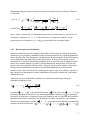
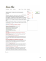
Figure 3.1. Aerial plot presenting the results of a sampling campaign following the 2005 DBL
152 spill near Port Arthur, TX. ....................................................................................................... 7
Figure 4.1. Principal causes of oil spills in the world, Source: ITOPF, 2009................................. 9
Figure 4.2 . Case-based fractions of oil spilt that undergo processes in the seawater and the
atmosphere. Source: Cedre, 2009. ................................................................................................ 10
Figure 4.3. Distribution of physical variability assuming perfect information, or no uncertainty,
and predictive Bayesian distributions based on limited data, and limited data with professional
judgment, showing the decrease in information entropy with increased information availability.
....................................................................................................................................................... 14
Figure 4.4. Graphical depiction of the Method of Images used in the SOSim model. ................. 22
Figure 4.5. Sketch of a Riemann sum concept with forward approximation to the function (the
value on the curve corresponds to the first discretization value of each element). ...................... 24
Figure 4.6. Representation of the superposition concept in three dimensions............................. 29
Figure 4.7. Recorded relative sunken oil concentrations evaluated subjectively, interpreted from
Figure 3.1. The spill occurred at 29.205° N, 093.4683° W as shown in Figure 4.8. .................... 37
Figure 4.8. General location of the DBL 152 spill, Scenario 1 .................................................... 38
Figure 4.9. Relative probability of finding sunken oil 12 hours after the spill. ............................ 39
Figure 4.10 Relative probability of finding sunken oil 17.5 days after the spill. ........................ 40
Figure 4.11 Relative probability of finding sunken oil 19.5 days after the spill. ......................... 41
Figure 4.13. Synthetic data on relative sunken oil concentrations in percent, for samples assumed
collected on two different days, (1) 6 days after the spill, and (2) 10 days after the spill. ........... 43
Figure 4.14. General location of the simulated spill scenario of Scenario 2 ................................ 44
Figure 4.15. Relative probability of finding sunken oil 8 days after the spill (1 day after the first
sampling campaign). ..................................................................................................................... 45
Figure 4.16. Relative probability of finding sunken oil 11 days after the spill (5 days after the
first sampling campaign and 1 day after the second sampling campaign), updated based on the
second data set. ............................................................................................................................. 46
Figure 4.17. Relative probability of finding sunken oil 13 days after the spill (3 days after the
second sampling campaign). ......................................................................................................... 47
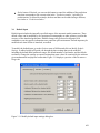
Table 4.1. Default parameter ranges included in SOSim, which can be edited by the user. ........ 16
Table 4.2. Input and output for Scenario 1 ................................................................................... 36
Table 4.3. Input and output for Scenario 2 ................................................................................... 42
1.0 Introduction
The ultimate impact of an oil spill stems from several factors, including its size, geographical
location, political and practical context of the response, as well as the occurrence of suspended or
sunken oil. Sunken oil can occur following a spill of heavy oil, or of lighter oil that entrains
sediment. The term sunken oil is used in this report to refer to oil on the bottom, though some of
the discussion and approach may also apply to oil suspended in the water column. As noted by
the Coastal Response Research Center (CRRC, 2007), "In the past few years, spills of nonfloating oil and oils that become submerged as a function of sediment entrainment have
presented significant response challenges and have resulted in enormous dollar-per-barrel
recovery costs. Currently, the ability to forecast submerged oil movement, estimate water
column concentrations of large droplets, and efficiently recover sunken masses in an
operationally expedient way is quite limited. Additionally, as this category of oil is difficult to
locate, track, and retrieve, managers have difficulty maintaining public confidence with regard to
response termination." Problems in locating and tracking sunken oil are further exacerbated by
the expense of developing and deploying new remote sensing techniques, and because some oils
may re-suspend and sink with changes in salinity, sediment load, and temperature.
Many models have been used to simulate the drift and fate of oil slicks in one, two, or three
dimensions using Eulerian or Lagrangian modeling techniques (Ojo et al, 2007; Spaulding et al,
1994; Spaulding et al, 1997; Beegle-Krause, 2001; Yapa, 1994; Sugioka et al, 1999). The spilltrajectory model developed and used most recently by the National Oceanic and Atmospheric
Administration (NOAA) is the General NOAA Oil Modeling Environment (GNOME),
developed by the Hazardous Materials Response Division (HAZMAT) Office of Response and
Restoration. GNOME includes statistical capability in the form of Best Guess and Minimum
Regret solutions (Galt, 1998). However, existing models are not developed for the detection and
mapping of sunken oil. Other possible approaches to locating and tracking sunken oil include
electro-acoustic detection, mechanical detection, and inspection by divers, as summarized in the
Technical Guidelines on Sunken Oil Assessment and Removal Techniques (NOAA, 2006).
However, integrated models for short and long-term sunken oil tracking with on-scene
calibration capability during emergency response have been identified as research needs (CRRC,
2007).
The occurrence of sunken oil is difficult to predict in time and space before, during, and after
cleanup, using either contaminant transport models or field data, for two reasons. First,
hydrodynamic or particle tracking models may be difficult to deploy and calibrate for tracking of
sunken oil, due to the site-specific and potentially transient nature of sunken oil occurrence and
location under changing field conditions, and limitations in the available information on
advective/dispersive forces acting on sunken oil. Second, the collection of field data on sunken
oil locations is intrinsically expensive. Modeling techniques that accept near-real time field data
as input and account quantitatively for both uncertainty and variability are not well-developed,
and have not been available to support response, cleanup, and damage assessment decisions.
1
The use of Bayesian modeling techniques to incorporate non-numerical types of information in
probabilistic assessments has exploded in recent years due to the development of new
computational approaches (e.g. Markov Chain Monte Carlo). The approach allows integration of
available numerical data together with any less-quantitative information, with rigorous
accounting for uncertainty in accordance with the laws of probability. Therefore, it represents an
approach to exploiting available field data on sunken oil locations together with estimated ranges
of values for coefficients of advection and dispersion. The Bayesian approach involves inclusion
of non-numeric information to develop posterior probability distributions for the uncertain
parameters of probability distributions for uncertain quantities of interest.
Predictive Bayesian methods involve the development of unconditional probability distributions
for the quantity of interest, by integrating over all possible values of the uncertain parameters
(expressed by the posterior). The approach has been used in oil spill prevention and preparedness
planning (Obie and Englehardt 1996; Douligeris et al., 1998) and for other applications including
hurricane, environmental, health, and safety risk analysis (Aitchison and Dunsmore, 1975;
Englehardt, 2004, 1995; Bloetscher et al., 2005; Englehardt and Swartout, 2004; Englehardt et
al., 2003; Anex and Englehardt, 2001; Englehardt and Peng, 1996). For example, a predictive
Bayesian compound Poisson model was developed to forecast changes in oil spill volumes
onshore in the Gulf of Mexico in response to proposed changes in oil transportation and response
equipment and policies, given geographically-defined historical oil spill data, shipping routes
and volumes, and hydrodynamic modeling results (Obie and Englehardt, 1996; Douligeris et al.,
1998). However, the approach has not been brought to bear on the problem of locating sunken
oil.
This project addresses current limitations in techniques for locating sunken oil on relatively flat
bay bottoms. The intended audience is oil spill emergency response professionals, and those
involved in oil spill recovery and remediation. Beneficiaries of the research are expected to
include the National Oceanographic and Atmospheric Administration, oil spill responsible
parties, and the oil spill response and recovery communities.
2
2.0 Objectives
Given the site-specific nature of the occurrence of sunken oil and the need to project its location
in time, a statistical data-limited technique representing a cross between a statistical static
sampling plan and a contaminant transport model was proposed for development in this project.
In discussions with the project advisory group, it was determined that information on bottom
“currents” and their potential forcing of the movement of sunken oil was too limited to be a
primary source of input information for the model. Rather, the capability to exploit limited field
data collected following a spill was desired. It was also agreed that the model should be
developed as a stand-alone, open-source, executable application with graphical user interface
(GUI), for possible incorporation in future oil spill response software.
To meet current needs in terms of locating sunken oil during emergency response operations, the
objective of the project was to develop a stand-alone, open-source, executable model with GUI,
with capability for:
1. Assessing sunken oil locations based on limited available field data collected shortly after a
spill event,
2. Projecting oil location in time based on subsequent limited field data together with shoreline
boundaries and the values or estimated ranges of values of the coefficients of advection and
diffusion, and
3. Providing updated projections based on additional field data as they become available.
Specifically, a predictive Bayesian multimodal Gaussian model of sunken oil locations across a
relatively flat-bottomed bay was proposed, to accept possibly irregularly-sampled field data at
times shortly after each spill event when sunken oil has appeared on the bottom. The calibrated
model also was to have capability for accepting input in the form of ranges of parameter values
based either on hydrodynamic data or professional judgment, to over-ride default ranges
assigned in the research. In that way, limited field data can be integrated with certain other types
of information to assess and project the location of dispersing sunken oil masses both before and
after cleanup begins, for spill response and decision-making, cleanup, and damage assessment.
Finally, it was agreed that the model should be capable of being enhanced in the future to accept
bathymetric information as input.
Based on discussions with project advisers, the scope of the project was limited to:
Sunken oil;
Relatively flat bay bottoms, dredged bays, reef flats and lagoons or pools protected by
offshore rocks; bays with steeply sloped bottoms would require capability for the use of
bathymetric data as prior information, a possible future enhancement;
Resolution down to the scale of the tidal excursion (oil locations effectively averaged
across this excursion);
Discrete accidental oil releases (as opposed to natural, progressive oil seepage);
Relatively uncomplicated concave and convex shoreline geometries; modeling in straits,
inland water bodies, harbors, islet areas, and like geographies are not addressed due to
computational limitations and the sometimes transient nature of small-scale features.
3
This report describes the development of the Sunken Oil Simulation (SOSim) model, to be used
for identifying sunken oil hotspots, tracking sunken oil following a spill, targeting cleanup
activities, and supporting cleanup termination decisions. The final product of the project is a
computer executable stand-alone software package created and tested under Microsoft Windows
32 bit operative system, programmed in the Python language and embedded in its own GUI.
Included in this report is a user‟s manual for the open-source product (Appendix A). Because the
model was developed using only open source software and GPL derivatives, its use is governed
under the GPL (General Public License) license terms (see license terms included in the source
code, Appendix A). This tool will allow the response coordinator to choose and customize
response options, including actions at the source, at sea, near the shore, and onshore, plan
operations at predetermined times and locations based on projected sunken oil locations, and
plan the overall cleanup and recovery phase to mitigate impacts.
First, current information reported in the literature and relevant to the transport of sunken oil is
reviewed and, based on that information; a conceptual model for development of the software is
presented. Then, the mathematical and computational aspects of the model are developed.
Finally the results of model verification versus real and synthetic data on sunken oil location are
presented, with conclusions regarding application of the model as a predictive, decision-making
tool.
4
3.0 Methods
The project was organized according to three essential tasks, as follows:
1.
3.
Development of an understanding of the factors relevant to the modeling of sunken oil fate
and transport, particularly as related to the bathymetric characteristics of bays for which a
Gaussian modeling approach would be applicable,
Development of a computational approach that would allow a highly parameterized
predictive Bayesian multimodal Gaussian model of sunken oil location to be executed on a
desktop or workstation computer,
Verification of the model versus real and synthetic sunken oil location filed data.
3.1
Task 1 Methods
2.
The objective of Task 1 was to compile and summarize data on the occurrence and transport of
sunken oil as reported for previous spills, and to synthesize input knowledge from the Research
Team to develop a conceptual approach for the model. Thus, the team gathered information from
the literature and oil spill response professionals including the project advisory team to (a)
evaluate possible methodologies and approaches, (b) understand the processes of hydrodynamic
fate and the transport governing the behavior of sunken oil mass as a basis for development of
the conceptual model and specification of default values and/or ranges of values of model
parameters, and (c) determine appropriate the geographical scale and resolution for the model.
Simultaneously, regular meetings with the project advisory team were held to discuss and
develop a conceptual model for development of the mathematical and software models.
3.2
Task 2 Methods
The objective of Task 2 was to develop a multi-modal predictive Bayesian Gaussian statistical
model of sunken oil locations across a bay that would accept spatial field data on sunken oil
mass following a spill, to project assessments of sunken oil locations in time. Input data for the
algorithms were to include field data collected after oil has begun to sink at and around a spill
site, dates of spill occurrence and sampling campaign(s), and shoreline conditions if applicable
for the desired modeling zone. Algorithms were to infer Bayesian posterior probability
distributions for uncertain model parameters describing the dispersion and movement of sunken
oil patches in time.
The multimodal aspect of the Gaussian model was needed to accommodate oil accumulating in
multiple areas of the bay as a result of localized sediment entrainment, localized bathymetric
catchment areas, and other effects. This capability was provided by superimposing multiple 2-D
Gaussian patches in the model. Each patch was assigned a weighting parameter, representing the
fraction of the total sunken oil contained in that patch, with all fractions summing to an arbitrary
constant value of unity representing the unknown total sunken oil mass. Because the total mass
5
of sunken oil was not expected to be known, the output of the model is referred to as relative oil
mass. Thus, the traditional requirement for normalizing the area under the Gaussian distributions
to a value of unity was not necessary and was relaxed. Because of the lack of a need to normalize
individual Gaussian distributions, there was no need to normalize the likelihood functions used
to develop the Bayesian posterior distributions, as will be described in Section 4 (Results).
Therefore, Markov chain Monte Carlo (MCMC) computation was not required. Because of the
computational demands of MCMC methods, the likelihood that the approach would not be
successful for such a highly-parameterized model, and the relatively unskewed and regular
nature of the parameter distributions to be integrated, it was decided to use a straightforward
Riemann sum to obtain the final predictive result. Modeling techniques and advances developed
during the course of the research are described in Section 4 (Results).
3.3
Task 3 Methods
The objective of Task 3 was to verify the model versus available real sunken oil data, as
possible, and versus simulated submerged oil data, and disseminate software and results to the
national and international oil spill community via an actively maintained website. The need for
synthetic data for verification was identified, due to the limited nature of available sunken oil
data recorded after a spill. Thus, the model was first verified versus data interpreted from a
graphical presentation of spatially-defined qualitative data on oil spill concentrations on the
bottom of the Gulf of Mexico following the DBL 152 spill (Barker, 2009). In addition, synthetic
oil spill data hypothetically collected in two successive sampling campaigns for a double patch
of sunken oil in a nearshore area were generated statistically, and used to verify aspects of model
functionality including superposition, boundary effects, and multiple sampling times.
3.3.1 Use of Available Qualitative Sunken Oil Concentration Data
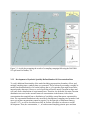
Data available for use in this project was obtained from NOAA for the DBL 152 spill, which
occurred on 11 November 2005 in the Gulf of Mexico. The data were available only in the
graphical form shown in Figure 3.1. Data were collected by dragging absorbent mop-like
samplers, termed pom-poms, along the bottom, and recording the geographical trace of the pompom and the visually-estimated amount of oil collected as ≤ 1%, 5-10%, 11-50%, 51-100%. This
figure was interpreted by assigning each recorded relative concentration in percent to the
midpoint of the drag trace shown in the figure. Coordinates of the spill location, also shown, and
sampling points were approximated based on the figure. The date of this sampling campaign was
taken as 25 November 2005, as indicated in the figure. No further information was available to
the project team, and therefore this information was taken as an example test case for the use of
limited information in a spill scenario.
6
Figure 3.1. Aerial plot presenting the results of a sampling campaign following the 2005 DBL
152 spill near Port Arthur, TX.
3.3.2 Development of Synthetic Spatially-Defined Sunken Oil Concentration Data
To verify additional functionality of the model including superposition, boundary effects, and
multiple sampling times, synthetic data was generated. This was done by assuming a roughly bimodal Gaussian distribution of oil on the bottom, that is, oil in patches (that might in turn have
internal patchy character). However, real oil spill data will not be neatly Gaussian in shape and
will come from a distribution of experimental error. Therefore, the bi-modal, bivariate Gaussian
distribution was used as the assumed mean oil concentration on the bottom, with relative
concentration then sampled from a distribution of variability around that mean, exponential in
form. The exponential distribution is the most likely distribution of sampling error around a fixed
mean, given that concentrations cannot be negative, by the Principle of Maximum Entropy
(Jaynes, 1957), as will be described more fully in Section 4 (Results) in reference to model
development. Thus, the concentration, C i , at each assumed sampling point in space and time
7
was sampled from an exponential error distribution with scale parameter
to a superimposed bivariate Gaussian distribution as follows:
and mean 1
equal
Mean concentration at the i-th of 90 (in space) x 2 (in time) samples was found by
2
N j , in
superposition of two assumed Gaussian patches of sunken oil, as Ci
j 1 j
which N
j
f j X, t | μ j , σ j ,
j
is the j-th assumed patch of sunken oil and
j
is the
relative mass of oil contained in that patch. The oil was assumed to occur in a nearshore
environment;
To account for real experimental and natural variability, measured sample
concentrations, C i , were then sampled from an exponential distribution with parameter
1 / Ci .
8
4.0
4.1
Results
Task 1 Results
4.1.1 Literature Review
The expression “oil spill” refers to a violent spillage of hydrocarbons concentrated in a specific
area, surpassing the natural assimilation capacities of the surrounding environment. Sinking is
the physical mechanism by which oil masses that are denser than the receiving water are
transported to the bottom. The oil itself may be denser than seawater, or it may sink by chemical
or physical means: chemically, the soluble fractions separate from denser fractions, leaving the
latter with the capability of sinking; physically, oil may have incorporated enough sand to
become denser than the water and therefore sink.
Vast quantities of crude oil and refined products are transported over long distances, incurring
constant and substantial risks of accidents. In particular, roughly one half of the oil consumed
worldwide is transported by sea, in ~9,130 oil tankers counted worldwide (ITOPF, 2009). High
vessel densities in maritime routes and loading/offloading ports, longer journeys, and intricate
aspects of geographical location all increase the risk of oil spills due to collision, negligence,
grounding, or defects in a vessel‟s structure. Insurance statistics indicate that most oil tanker
accidents resulting in marine oil spills result from human error, including “… badly handled
maneuvers, neglect maintenance, insufficient checking of systems, lack of communication
between crew members, fatigue, or an inadequate response to a minor incident …” (Cedre,
2007). From a more practical point of view, examination of the circumstances surrounding
accidents (ITOPF, 2004) indicates a high percentage of spills due to groundings and collisions.
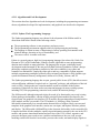
Figure 4.1 shows statistics on the reasons of oil spill occurrences.
Grounding
Structural damage
Fire, explosion
0%
10%
20%
30%
40%
Figure 4.1. Principal causes of oil spills in the world, Source: ITOPF, 2009.
The nature of oil transported by sea varies from the lightest oil (highly volatile hydrocarbon or
gasoline) that floats on the sea water and evaporates to the atmosphere, to heavy fuel oils, of
which perhaps only 10% will evaporate (ITOPF, 2009) with much of the remainder sinking to
the bottom. Processes that affect sinkable oil mass following a spill include evaporation, water
9
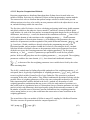
and oil mixing and sedimentation. Figure 4.2 shows case-based examples of the approximated
fractions of spilled oil mass that undergo evaporation and all other processes in seawater.
100%
80%
60%
40%
20%
0%
Atlantic Aegean
Empress Sea
Ignition and Fire Occurred
During Spill
Prestige Amoco
Cadiz
No Ignition
Occurred
Figure 4.2 . Case-based fractions of oil spilt that undergo processes in the seawater and the
atmosphere. Source: Cedre, 2009.
In general, crude oils and certain heavy refined products and sludge deposits have the potential to
sink, with sinking of oil generally becoming important from 1-8 days following a spill (Coastal
Response Research Center, 2007). Sunken oil then accumulates on the bottom in reported
thicknesses of about 2.5 inches, regardless of the size of the oil patches (Beegle-Krause et al.,
2006). Sedimentation of thick and heavy oil occurs rapidly, and involves the majority of the oil
minus a small percentage (< 10%) that evaporates and a portion that remains in bubbles in the
water column for a short time. Evaporation and mixing with water diminish the sinkable fraction,
while sediment entrainment increases sedimentation. Incorporation of water into the oil mass due
to mixing may prevent sinking for periods of hours to days following the spill. For spills of light
oil, sedimentation generally occurs over a long period of time and involves < 5% of the oil mass
(Cedre, 2007).
Sinking of heavy oils (API gravities less than ~7.0) due to gravity is more likely in quiescent
seawater where currents are under 0.1 knot (Research Planning Inc., 2001) because higher
currents typically keep oil droplets suspended in the water column longer. According to NOAA
event comparison charts, oils denser than local water have not been observed to impact the
shoreline unless the source of the oil was within the surf zone or the oil moved into relatively
denser water and thus became buoyant (Beegle-Krause et al., 2006). From Protocols for NRDA
Surveys (Research Planning Inc., 2001), "... sunken oil can be buried by silt in harbors or sand in
offshore areas within days to weeks. Once buried, it can remain for years, only to be exposed by
storms or dredging operations." If near shore, sunken oil and tar can wash up on beaches
following storms for years following a spill. Gravity will induce flow of the oil in the offshore
direction, towards deeper water (Beegle-Krause et al., 2006).
10
As reported in Protocols for NRDA Surveys (Research Planning Inc., 2001), heavy oil can
temporarily accumulate in low-flow zones. In rivers, accumulation may occur in backwaters,
sloughs, inactive scour pits, and in the lee of point bars, wing dams, and other man-made
obstructions. In estuaries, potential accumulation areas include man-made depressions (e.g.,
dredged channels, marinas and boat slips, prop scour pits, turning basins), natural scour pits
active during periods of high flow, and abandoned channel meanders. Along the outer coast,
accumulation may occur in troughs between offshore bars, lagoons or pools protected by
offshore rocks or coral, reef flats protected by reef crests, and in the lee of any obstruction of
currents along the coast (e.g., rocks, jetties, and breakwaters).
Oils lighter than the receiving water may sink by (a) adhering to sand-sized particles during
mixing in the surf zone; (b) stranding on shore, picking up sand, then being eroded from the
beach by waves and deposited in the near-shore zone; and (c) adhering to the substrate during
low water, then not re-floating when water levels rise. The latter mechanism is more likely in
rivers and streams where water levels may fluctuate. In general, sunken oil that is intrinsically
lighter than surrounding water (i.e., that sank by mixing with sand) can re-float if the oil
separates from the sand or bottom substrate. Such separation may occur upon warming, due to
the reduction in viscosity.
Sedimentation is of significant concern even if the oil has a light density, if a spill occurs in a
nearshore environment where the oil can mix with sand or sediment causing it to sink, as
happened in the Braer, Erika and Prestige incidents (ITOPF, 2009). In such cases the sunken oil
is extremely difficult to detect and recover. In general, once on the bottom, most hydrocarbons
easily enter gaps and flow by gravity so deep that it may be impossible to find by inspection.
Sunken oil mats tend to remain stationary in the absence of storms; local bottom currents
typically do not have enough energy to move the mat. Release and resuspension of parts of
submerged oil mats by long period gravity wave energy occurs most often along the near-shore
shelf where water is shallower and wave energy extends closer to the bottom depth (Dean and
Dalrymple, 1991). As a result of this increasing tendency to remain stationary following
deposition in deeper water, the mats tend migrate in the offshore direction over time (BeegleKrause et al., 2006). If the mat is broken up into particles during mixing, it does not tend to recoalesce. There is a significant difference in the oil content of oil masses that sink by gravity and
those that sink by entrainment and sedimentation. The former may contain only a few percent
sediment, whereas oil-contaminated sediments accumulated on the seafloor generally contains
less than 1% oil (Research Planning Inc., 2001).
Hydrocarbons that are not removed from certain ocean bottoms can seriously damage
populations living within the sediment substrate. Sunken oil weathers slowly; therefore toxic
components can persist and be a source of exposure during re-floatation or benthic transport. A
spill of heavy fuel oil is likely to cause much more damage than a crude oil spill of a
corresponding size. The duration of spillage also plays an important role. A sudden violent
release will concentrate the effects on a smaller area as compared with a long, slow leak.
11
Several properties affect the classification of oil as heavy or light, and consequently can modify
the propensity of the oil to sink as explained above. These combined properties, including
density, viscosity, pour point, solubility, chemical composition and potential for emulsification,
along with associated short-term behavior in the environment and impacts to natural resources
(Research Planning Inc., 1994), allowed for the classification of oil into six broad categories. In
general, Type 1 oils are very light, including gasoline and very volatile hydrocarbons. Type 2 are
moderately volatile and soluble, including jet fuels, diesel fuel, number 2 fuel oil, and light crude
oils. Type 3 oils include most crude oils, known by their persistence and diminished propensity
to evaporate (about one third of the total mass evaporates within 24 hours). Type 4 oils may have
little propensity to evaporate or dissolve, and high likelihood of sinking. Type 5 oils have
essentially no evaporation potential, weather very slowly, and sink immediately, including heavy
industrial fuel oils. Type 6 oils include heavy animal or plant oils. This classification of oils is
tightly related to API gravity, a measurement of the relative density of petroleum liquids
developed by the American Petroleum Institute and adopted by the oil industry worldwide. Type
1 oils may have API gravities around 31 °API, whereas a Type 4 oil can have an API gravity of
less than about 10 °API, in which case the oil will typically sink in water.
Transport and Accumulation
The following points concerning characteristics of the initial fate and transport of sunken oil
have been excerpted, adapted, interpreted, and/or condensed from the references cited:
After events of high bottom energy, sunken oil can be resuspended and sometimes mixed
until it is broken up into small globules. These smaller globules of heavy oil are not
expected to coalesce into a larger slick at some later time (Beegle-Krause et al., 2006),
but rather to weather and degrade over long periods. At depth, the so-called “convergence
zones” found in the surface are not found, and a mechanism for bringing the globules
together no longer exists in the bottom (Beegle-Krause et al., 2006);
Long-term transport of heavy oil is seldom compared to long-term sediment transport on
continental shelves. Events with sufficient energy are more likely to be caused by longperiod waves than by the local bottom currents (Beegle-Krause et al., 2006); and
Sediment is typically transported greater distances along the shelf than across the shelf
(Beegle-Krause et al., 2006). This observation could represent prior information for the
development of Bayesian prior probability distributions for coefficients of advection and
dispersion in directions perpendicular and parallel to shore.
Mechanisms of Resuspension of Sunken Oil
When a high-density oil spill occurs, a large portion of the oil will sink to the bottom to form
large discrete mats in many areas and smaller globules in others (Beegle-Krause et al., 2006).
Here, the term “globule” is equivalent to “tarball”, also used in the literature. Observational data
in NOAA data bases suggest that oil remains in areas of heavier concentration until high-energy
storms redistribute the oil. The following are excerpted or adapted from Beegle-Krause et al.
(2006), except as noted:
12
Literature suggests that average current conditions will not be sufficient to move the oil
in a continuous manner (Beegle-Krause et al., 2006; Boehm et al., 1981). Rather, “The
oil will remain stationary on the bottom until an event occurs with enough energy to stir it
up into the water column;”
“Tarmats occur when floating oil moves into the surf zone, collects sediment, and sinks;”
“With enough energy, tarmats in the bottom generally break up into smaller pieces of oil
that spread out into a large area. Otherwise, the tarmats remain stationary and intact;”
“Outside the inner shelf, where coastal current jets form, long-period waves will be the
only source of turbulent energy at the bottom other than large storms strong enough to
mix the entire water column;”
“The oil will behave similarly to local sediments in terms of episodes of burial and reexposure and mobilization into the water column;”
The energy required to move the oil varies with depth and site and is unknown. A breakup energy level has been estimated as 6 m2/Hz (Beegle-Krause, et al., 2006).
4.1.2 Conceptual Model
The literature review developed in this task was used together with discussions with the project
advisory team (Christopher Barker, NOAA Office of Response and Restoration, Emergency
Response Division and Assessment & Restoration Division, Technical Liaison; Nancy Kinner,
Co-Director, Coastal Response Research Center, University of New Hampshire; Amy Merten,
Co-Director, Coastal Response and Research Center, NOAA) to develop the conceptual model
targeting end user needs. The initial concept was a predictive Bayesian superimposed 2-D
Gaussian model incorporating computer algorithms to allow estimation of the highly
parameterized model given limited numerical data and possibly additional information on the
surroundings after the oil has begun to sink. As a result of Task 1, it was decided to develop a
stand-alone, open-source model with graphical user interface. The model was to be capable of
accepting limited available field data on oil spill concentrations, whether quantitative or
qualitative in nature, sampled randomly in space, from multiple sampling campaigns, and to
include default ranges for coefficients of advection and dispersion in two horizontal directions.
Additional model input would include the time and location of the spill and of all oil
concentration data.
4.2
Task 2 Results
Predictive Bayesian distributions are distributions of unconditional (on knowledge of the
parameter vector) probability. The predictive distribution is obtained by multiplying the
sampling distribution (e.g., the multinormal), by a Bayesian posterior distribution describing
numerical and other knowledge of the parameter vector, and integrating the product over the
uncertain parameter space according to the Theorem of Total Probability. The result is a
distribution that evolves in shape, becoming progressively narrower as the level of available
13
information increases, converging on the underlying distribution of variability. Figure 4.3 shows
this evolution in a general, one-dimensional case.
Figure 4.3. Distribution of physical variability assuming perfect information, or no uncertainty,
and predictive Bayesian distributions based on limited data, and limited data with professional
judgment, showing the decrease in information entropy with increased information availability.
The general predictive Bayesian analytical model that represents the unconditional probability of
a particle of oil at X x, y is the following expression, in which the integration is over an
uncertain parameter space:
J
f( x, y, t )
j
f j ( x, y , t |
x, j
,
y, j
,
x, j
,
y, j
,
j
) L Ci | μ, σ, ρ, γ
μ σ ρ γ
(4.1)
j 1
in which f j (X, t | μ j , σ j ,
parameters mean μ j
sunken oil fraction
j
) is the j-th Gaussian patch given knowledge of the range of
μ x μ y j , standard deviation σ j
j
, with
j
σ x σ y j , correlation coefficient
1 to maintain conservation of mass; μ j
j
, and
v j t ; v j is the
14
2
j
2Dt is the standard
deviation or measure of the effective “breadth” of the patch at time t ; D is the horizontal
average sunken oil dispersion coefficient (L2/T); and L(Ci | μ, σ, ρ, γ) is the likelihood function of
the observed concentration data, Ci , at the irregular sampling locations and times, in which Ci
represents the vector of relative concentration data, (C1, C2,…,Ci, … CI), at locations (xi, yi) and
times, ti. The parameter space is described as follows:
average velocity vector (L/T) of the j-th Gaussian patch; t is time (T);
μ {(
x
,
y 1
σ {(
x
,
y 1
) ,..., (
x
,
y J
) ,..., (
x
,
y J
{ 1 ,...,
{ 1 ,...,
J
J
) }
) }
}
}
(4.2)
Note that one of the patches has no
parameter since
4
1- (
1
2
3
)).
In essence, field data are sampled from a distribution of sampling variability around a mean
concentration. This mean is modeled by the value of the multimodal 2-D Gaussian distribution at
that point in space. The distribution of sampling variability was assumed to be exponential in
form, because the maximum Shannon entropy distribution around a fixed mean over a nonnegative range is exponential (Shannon, 1948). This form is proposed as the most likely
distribution of concentrations that might be observed at a point on a bay bottom, by the Principle
of Maximum Entropy (Jaynes, 1957). That is, entropy is the average log of the inverse height of
the density and so, assuming normalization, is a measure of distribution “breadth.” Therefore,
maximizing entropy means maximizing the range of feasible outcomes and, all-the-more-so, the
number of ways to satisfy the constraints. The ME distribution is then realized because it can be
obtained in overwhelmingly many more ways. For example, the Gaussian diffusion equation
itself results if the entropy of a distribution of diffused mass is maximized subject to independent
constraints in terms of the mean (or advective velocity, controlled by pressure gradient) and the
variance (or coefficient of diffusion, controlled by e.g. viscosity, temperature). Likewise, entropy
can be the starting point in deriving many physical laws, if the governing constraints are known
(Kapur 1989; Jaynes 1957).
Assuming an exponential distribution of oil concentration sampling variability around the mean,
modeled by the multimodal Gaussian distribution, the likelihood function in Equation 4.1 can be
written in terms of the relative concentration as follows:
L(Ci | μ, σ, ρ, γ )
I
i 1
exp(
Ci )
(4.3)
15
in which 1
J
j 1
j
f j ( xi , yi , ti | μ j , σ j ,
j
) . That is, it is assumed that the concentration
sampled at a point in space and time comes from an exponential distribution of sampling error
with mean 1/ .
The conceptual model, though Bayesian in character to address uncertainty and speed of
computation, was developed primarily to accept field (sampling) data. Due to its structure, the
capability for accepting prior information such as derived from bathymetry or professional
judgment regarding model parameter values can be added as appropriate. Particular terms in the
model are described in more detail in the following sections.
4.2.1 Assumed or specified parameter domains
It was determined in discussions with project advisors to design the model with capability for
operation without specific information on average water velocity vectors and diffusion
coefficients found on the bay bottom. Accordingly, default ranges of values were assigned for
each of these parameters. The model uses these ranges as the ranges of integration for Equation
4.1. Default ranges are wide, as shown in Table 4.1, having been assigned based on literature
values and initial confirmation runs, together with a margin of uncertainty. It is expected that
default ranges can be refined further in the future. In addition, the SOSim model is equipped with
an Options menu that can be used to change and set up the built-in default parameter ranges
shown in Table 4.1.
Parameter
Velocity in the east-to-west direction
Symbol
vx
Units
km d
Minimum Maximum
-3.0
3.0
Velocity in the north-to-south direction
Coefficient of diffusion in the east-to-west
direction
Coefficient of diffusion in the north-to-south
direction
Coefficient of correlation between directions
Mass conservation weighting parameter
vy
km d
-3.0
3.0
Dx
km2 d
0.01
1.1
Dy
km2 d
0.01
1.1
[-]
[-]
-0.999
0
0.999
1
Table 4.1. Default parameter ranges included in SOSim, which can be edited by the user.
4.2.2 Conditional bivariate Gaussian distribution
Mass concentration in a fluid subject to advection and dispersion in any media can be shown, for
example by maximizing the Shannon entropy of a distribution of (oil) particles subject to a mean
location and variance, to have a Gaussian concentration profile subject to bounds with real mean
and real positive variance domains (Shannon, 1948). Conditional on knowledge of the parameter
vector, a bivariate Gaussian is adopted as the conditional sampling distribution for the two16
dimensional Bayesian model of sunken oil locations on a relatively flat bay bottom. Therefore,
we have that:
f j ( X, t | μ j , σ j ,
j)
1
N X, t |
j
2
in which Bm
xm
2
x0
x
2
x, j
xm
y, j
x0
2
x
2
1
x
ym
y
y0
(4.4)
2
21
j
x
Bm j
exp
j
y
ym
2
y0
y
2
y
and μ j and σ j represent the two dimensional means and covariance matrices, respectively, for
each patch. In Equation 4.4, x m , y m are the coordinates of a point to be modeled, and
represents the set of parameters μ j , σ j and
j
as described in the conceptual model.
4.2.3 Bayesian posterior distribution
Bayesian methods involve first assigning a joint (that is, multivariate, to address all uncertain
parameters) prior probability distribution to the uncertain parameters of a sampling distribution
such as the Gaussian. This distribution is assigned based on non-numerical forms of information,
such as bathymetry that might affect sunken oil locations. In the model developed, no prior
information was assumed, such that the probability prior to data collection of finding oil on the
bottom was constant spatially (for relatively flat ocean bottoms, dredged bays, reef flats and
lagoons or pools protected by offshore rocks). Therefore, based on the Principle of Maximum
entropy, the prior distribution was taken to be a uniform distribution over the uncertain
parameter space. This can be done by setting the prior equal to unity as an arbitrary constant, so
that it drops out of the equation, because normalization if required is obtained in a subsequent
mathematical step.
A Bayesian posterior distribution is obtained as a refinement (narrowing) of the prior
distribution using Bayes Law:
f
| x1 , x2 , ..., xI
L x1 , x2 , ..., xI |
g x1 , x2 , ..., xI
,
(4.5)
in which L x1 , x2 , ..., xI | is the likelihood function,
is the prior, and g x1 , x2 , ..., xI is the
probability that the data was observed, a normalizing constant with respect to . As mentioned
previously, the total mass of sunken oil is generally unknown, and as a result the final predictive
distribution need not be normalized, as a distribution of relative, not absolute, concentrations.
Therefore, the normalizing constant, g x1 , x2 , ..., xI , is also not needed, and the (un-normalized)
( ) L x1 , x2 , ..., xI | .
posterior for the model becomes f ( | x1 , x2 , ..., xI ) L x1 , x2 , ..., xI |
17
4.2.4 Multimodality and Superposition
The model was developed as a multimodal Gaussian, to account for example for the presence of
multiple patches of oil collecting on the bottom, or for oil concentrating more highly in deep
bathymetric features at any or all times. The predictive model is able to infer from the data
whether or not the sunken oil is distributed in single or multiple patches, and to track and predict
this multimodal behavior in time. As a consequence, the assessed concentration profile can be, or
become, either multimodal or unimodal in time. Results depend upon the data, as well as on
boundary conditions, desired prediction times, and the resolution selected by the user.
The total mass of sunken oil is not typically known as a function of time, considering ongoing
sinking and re-suspension processes. Therefore, computations of the model arbitrarily assume a
constant mass of sunken oil with time, producing maps of relative sunken oil in space which
identify areas with the most oil. As such, relative masses cannot be compared across time.
Therefore, in an emergency response scenario, the occurrence of increases or decreases in the
total mass of sunken oil over time would need to be assessed from the field data, for example, by
inspection. With this basic assumption, the model can infer the relative mass of oil contained in
each patch from the field data. This relative mass is represented by the parameter j ,
representing the fraction of total sunken oil that belongs to the j-th patch, which can be
considered the mass weighting parameter among patches. Summation of the j to a constant
value over time was therefore one important test of internal model consistency used for verifying
the model as it was developed.
An expansion of the Bayesian Bivariate Gaussian analytical expression for multiple modes
shows how superposition is mathematically attained in the model:
f (X, t | ) overall
j
N X, t |
j
,
j
1
(4.6)
That is, the overall conditional Gaussian sampling distribution is composed of the sum of any
possible combinations of a weighting parameter, the fraction j , among patches and a bivariate
normal distribution N j with parameters μ x j , μ y j , σ x j , σ y j and
j
, that represents a single
mode or oil patch j , such that the sum of the weighting parameters is equal to one. To maintain
this sum equal to unity over multi-dimensional integration operations with some computational
efficiency, an algorithm based on combinatorial mathematics was developed, as described in the
section Algorithm and Code Development.
18
4.2.5 Projecting the oil mass in time
The concentration profile in a (one dimensional) media following the instantaneous introduction
of a mass, M, can be found either starting with the Fick‟s Law-based advection-diffusion
equation and applying the inverse Fourier transform (Chin, 2006), or solving the random walk
model for a particle (of oil) (Einstein, 1925). The result takes the form of a Gaussian distribution
with variance growing in time:
c x, t
M
A 4 Dx t
exp
x0 vt
4 Dx t
2
,
(4.7)
in which D x is the uncertain diffusion coefficient of a Gaussian path in one dimension [L2/T], vt
is the distance the mass M has traveled from the initial point x , v is the uncertain mean
velocity vector of the Gaussian patch [L/T], and A is the transverse area of mass introduction. In
the model developed, the mass per unit area, M/A, of sunken oil is taken as an arbitrary constant.
Comparing the fundamental solution of the diffusion equation (Equation 4.7) to the equation of a
2 Dt .
Gaussian distribution (Equation 4.4 in one dimension), it is seen that
vt and
Furthermore, by the time an oil mass reaches the bottom of the sea from the initial aerial spill
location ( x0 , y 0 ), it will already be characterized by an initial velocity and an initial diffusion
coefficient, which results in:
μ
v0
vt
and
σ σ0
2Dt
(4.8)
Equations 4.8 contribute uncertain parameters to the likelihood function which vary with
sampling time, and to the Gaussian model which vary as a function of user-defined times of oil
mass prediction.
4.2.6 Taking Into Account the Potential for Sinking and the Short-Term Weathering
The SOSim model infers oil location as a function of time by comparing the initial point of
accumulation with data on its distribution at a later point in time. If only one sampling campaign
is available, the initial point of accumulation is critical to these predictions in time. While many
times the spill location and time are known, and may represent the initial point of accumulation
for floating oil, the initial time and point of accumulation are not as well known for sunken oil,
depending on oil density, sediment entrainment, and other factors. In fact, while oil may take a
week or more to start a weathering process that may result in sinking, Type 4, 5 and 6 oils start a
process of sinking by gravity immediately after abrupt release or during a continuous spill event
(each oil type at its own pace).
For the SOSim model, the initial spill time is indicative of the major release at the actual
coordinates of the accident at the surface, but the approximated time at which oil starts to collect
19
at the bottom is really what defines the framework of the model with respect to time. The
difference between the spill time and the time at which oil starts to collect at the bottom is
considered a “retardation factor”, included in the model as a function of the oil type as identified
by the user. Oil is identified as one of the accepted Types 1 through 6 described in the literature
review, accounting for multiple properties of oils related to the potential for sinking by gravity
and for weathering by evaporation and/or dissolution. Accordingly, all times that modify the
likelihood of finding sunken oil at a given location are adjusted by the retardation factor, RF, as
t t RF , in which RF reflects an assessed, generalized delay associated with the particular oil
type before starting to collect at the bottom. It is assumed that no sampling campaigns will be
useful if performed before the assessed retardation gap.
4.2.7 Incorporating Multiple Sampling Times
In order to better account for changes in sunken oil movement due to e.g. tidal action, storm
events, and sediment entrainment, the model was built with capability for accepting data from
multiple sampling campaigns (sampling campaigns performed at different times and different
areas). Input of data subsequent to the initial sampling campaign increases the number of product
terms in the likelihood function, increasing the information content and increasing information
concerning oil movement, in particular.
The likelihood function of the observed data, Ci, at each i-th irregular sampling location and
times with respect to the uncertain parameter space is:
L(Ci | μ, σ, ρ, γ )
I
i 1
exp(
Ci )
(4.3)
in which Ci represents the vector ( C1 , C 2 ,..., Ci ,...C I ) of measured concentrations at different
location-times. The SOSim GUI allows up to ten different sampling campaigns or times, with an
unrestricted number of sampling locations at each time.
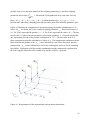
4.2.8 Development of Boundary Capabilities by the Method of Images
The method of images (or method of image charges in electrostatics, or reflection theory in
physics) was used in the SOSim model as a numerical approach to calculate the reflection of
sunken oil from shorelines in nearshore spill scenarios. The physical reality of the ocean
boundaries (the shoreline) is approximated to an ideal condition in which a “relatively-flat ocean
bottom” is truncated by a theoretically vertical barrier that is assumed to retain the sunken oil
without compromising the oil‟s mass conservation and the Fickian nature of the transport
process; that is, it is assumed that phenomena that might occur close to a shoreline environment
such as oil adsorption onto the barrier‟s material or flow into the porous medium do not occur.
Figure 4.4 replicates the physical approximation in one dimension. The method is used as a
numerical approach to calculate the effect of the vicinity of coastlines in oil spill scenarios.
20
The scheme used in this research also involves the assumption of uniqueness of the current
modeling conditions, maintaining conservation of mass, while redistributing it consistent with
each source and at each time within the nearby boundaries imposed by the geometry of the
coastal zone, approximated and projected to the bottom (see Figure 4.4). A novel implementation
using a polyline approximation of shoreline geometry was developed and implemented in
SOSim, as described in this section.
Consider an example in which an oil patch is denominated „the source‟. The source occurs at a
certain point ( x 0 , y 0 ) = ( x , 0) on the bottom of a bay and has a concentration distribution
c ( x, y ). This point lies at some distance x from the shoreline which, by definition, has a
concentration gradient of zero. As the patch approaches the shore, oil at the leading edge begins
landfall. It is then assumed that this oil mass is reflected back into the water, producing an
accumulation in the nearshore environment by the principle of superposition. In one dimension
the reflection is easily computed as a sum of the inflowing mass and the reflected mass.
However, in two dimensions when the shoreline is not straight, reflections are not perpendicular
with respect to only one line and calculations become cumbersome. Therefore, (relative) mass
accumulation is computed in SOSim by setting up imaginary conditions to replicate the curve of
the boundary. The method of images momentarily replaces the boundary by an “image source”
or a “reflection”, equal in concentration distribution but located at opposite coordinates (- x , 0)
across the boundary. This new situation is equivalent to the original layout because superposition
of the source and its reflection concentration distributions will simulate the zero concentration
gradient at the boundary and will account for spreading and contention of oil. The result is then
the summation of concentration distributions on the source side, and all results imagined to occur
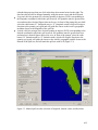
beyond the boundary can be ignored. Figure 4.4 depicts the concept.
21
Figure 4.4. Graphical depiction of the physical idealization of the boundary conditions to apply
the Method of Images in the SOSim model.
In the single boundary case described above, no other boundary has effect on any of the sources,
and thus reflection stops at once and the case is considered of zero order. When multiple
boundaries coexist, reflections are not perpendicular with respect to only one line but instead it is
assumed that they are perpendicular with respect to each segment of a boundary interpreted as a
series of connected lines, where every single source is reflected with respect to each of the line
segments. In the application of the method of images in groundwater hydraulics to modeling
flow near aquifer boundaries, the source is reflected with respect to each horizontal or vertical
aquifer boundary, and each subsequent reflection is in turn affected by the boundary that did not
reflect it before (Bear, 1979 and Todd, 2005). This approach to considering perpendicular or
parallel boundaries (that are not necessarily contiguous) was adapted and implemented for the
case of non-orthogonal contiguous line segments representing geographical boundaries to sunken
oil movement. That is, the requirement for perpendicular or parallel boundaries was relaxed
using a new method developed to address the change in correlation between the x and y
directions. The multi-reflection process creates a series of mass imbalances that must be
balanced back with further reflections. As a result, computation must be iterated to attain both
mass conservation and zero-concentration gradient values at the shoreline.
To approximate shorelines with polylines, the user is shown a map of the spill area, and
instructed to click on the map to define up to 10 vertices. These vertices are connected by
straight lines to approximate the shoreline contour. The algorithm allows the addition of as many
superimposed terms as needed to the conditional Gaussian bivariate distribution. However,
computational demands increase nonlinearly with the number of vertices, due to the nature of the
numerical integrations across the multi-dimensional parameter space and the combinatorial
numerical approach. Therefore, the program incorporates a limit of ten vertices.
22
This approach, like many numerical methods, requires a stopping rule to define the limit of
iteration needed to obtain an acceptable solution. In this research, it was found that the sum of
second and lower order reflections provided sufficient detail to obtain an observable mass
balance in the water body. Thus third and higher order reflections are neglected, greatly reducing
computational demands (currently model runs require several hours on desktop computers).
Also, because the Gaussian tail is mathematically infinite, reflection is calculated beginning
when a patch center reaches a distance of 2 from the shoreline, and ending when the tails of
the outgoing source and the incoming image have already “crossed” (refer to Figure 4.4) and no
longer sum to a value higher than the concentration at the mean 2
To prevent calculation of
sunken oil projections at times beyond the estimated time of landfall, when the patches would
appear to “bounce” off of the shoreline, a warning message is issued by SOSim when the
requested prediction time is estimated a priori to be beyond the time of landfall. Such prediction
times are beyond the reasonable capability of SOSim to assess relative concentrations.
4.2.9 Integration to obtain the predictive relative concentration profile
Several different integration techniques were considered for the multivariate integration
expressed in Equation 4.1. The first was an analytical solution, which is available for the
predictive Bayesian multinormal distribution (Aitchison and Dunsmore, 1975). However, no
solution is available for the multimodal analog, that would allow the inference of varying
numbers and weights of multiple patches of oil. Second, the use of Markov chain Monte Carlo
(MCMC) simulation was considered, to generate vectors of random variates sampled from the
Bayesian posteriors over which averages could be computed at each point in space and time.
MCMC is the most popular approach to computation of Bayesian posteriors. However, the
approach was not considered likely to estimate posteriors successfully, due to the high
dimensionality of the model, without the development of new computational approaches. In
addition, the principal advantage of the approach is the ability to compute the normalizing
constant for the likelihood function, not needed in the SOSim model. Moreover, the distributions
applicable to the uncertain parameters of a Gaussian distribution are not highly skewed, and are
therefore relatively easy to integrate as a discretized sum. Therefore it was concluded that the
most efficient approach would be a direct Riemann sum approximation. The approach involves
approximating the volume under a surface (or area under a curve) as a sum of small differential
volumes, partitioned over the domain of the parameter space. Figure 4.5 shows the basic
principle of the Riemann sum integration.
23
Figure 4.5. Sketch of a Riemann sum concept with forward approximation to the function (the
value on the curve corresponds to the first discretization value of each element).
The Riemann sum requires one initial input: the approximate domain of the uncertain
parameters. As mentioned, default values for this range are included in the model based on
literature information and statistical principles, and handled as explained in the section
Algorithm and Code Development. The Riemann sum integration, though simple in concept,
consumes considerable computational resources in the SOSim model because of model
dimensionality and the programming structure required in the Python programming language
used. Algorithms are explained under Algorithm and Code Development, including how the
resolution of the integration (the number of discretizations of each parameter range) are related
nonlinearly to the number of oil patches and to the precision of prediction.
4.2.10 Geographical Versus Modeling Units
Sampling campaigns should be recorded and accepted by the model in World Geodesic System
(WGS) units (degrees, minutes and seconds expressed in decimal degrees in the GUI prompts).
Interaction of the user with the canvas of the graphic user interface also results in operations in
WGS units, because none of the embedded maps are projected to a flat surface. Equations 4.4 to
3.8, on the other hand, all require distances in planar units (SI or metric system). Therefore,
conversions using the Universal Transverse Mercator (UTM) projection are used to translate
WGS input into distances in km that can be used in the diffusion, advection, and statistical
equations, and to convert gridded model output back to WGS format for graphical presentation
in map format. The process, other than involving the creation of global Python functions for the
conversions, engages certain computational algorithms to guarantee that (a) precision is not lost
in the double conversion process (error is on the order of 1e-9), and (b) operations over points
located at overlapping borders of UTM zones are correctly converted without affecting precision
and guaranteeing that user inquiries concerning the locations of sunken oil are accurately
displayed on the map canvas of the GUI application.
24
4.2.11 Algorithm and Code Development
This section describes algorithm and code development, including the programming environment
chosen, algorithms developed for implementation, and graphical user interface development.
4.2.11.1 Python: The Programming Language:
The Python programming language was chosen for development of the SOSim model in
discussions with NOAA based on the following criteria:
The programming software is non-proprietary and open source,
The programming environment supports relatively rapid prototyping and testing,
The language is robust in terms of functioning in various operating environments with
minimal damage, alteration or loss of functionality, and
The source code is viewable at all times.
Python is a general-purpose, high-level programming language first released by Guido Van
Rossum in 1991 in The Netherlands. Python is flexible, applicable to many programming
domains and available on many platforms. The language has an open, community-based
development model managed by the non-profit Python Software Foundation. Python‟s design
philosophy emphasizes programmer productivity and code readability (core syntax and
semantics are minimalistic, employing white spaces and easy commands). Python supports
multiple programming paradigms (primarily object oriented) and features a fully dynamic type
system and automatic memory management, similar to Perl, Ruby, Scheme, and Tcl.
The Python programming language has an open, general public license (GPL) that allows source
code modification, addition of original code as “imported” packages, and publication of derived
work (as GPL). Packages that are created around the world are available to the Python
community. Python has also been used as an extension language for many existing systems,
including GIS, Web programming, numerical tools, and the R statistical package.
The SOSim model, although using and relying for much of its functionality on several existing
Python packages and modules, consists of three principal Python modules developed by the
research team: the graphical user interface (GUI) module, the operating and processing interface
(OPI) module, and the core module. The GUI module (ui_SOSim.py in the electronic
deliverable) automatically lays out and retains characteristics of widgets, labels, canvases and
templates in the graphical user interface, retains raw user input, and imports Windows palettes
and display. The OPI module (SOSimOPI.py in the electronic deliverable) is the executable file.
It imports and links all other modules, captures input information entered by the user in the GUI
module, and operates interrelated buttons and activities of the GUI; it filters, organizes, and
processes the input; passes ready-to-use variables and attributes to the core code; accepts
modeling results back from the core module; processes the results; and sends display signals to
25
the canvas layout of the GUI module to allow it to depict relative sunken oil concentrations on a
map for further user interaction. It also controls modal behavior of the main windows, pop outs,
menus and toolbars. The core module (SOSimCore.py in the electronic deliverable) uses
variables and attributes passed by the OPI module to compute the predictive Bayesian relative
concentrations, saves output files, and passes results back to the OPI module for display by the
GUI or for further use. The GUI has the capability to communicate with the core module through
the OPI module during a model run, after a predictive result has been presented, to allow the user
to request the modeling of contiguous or other areas as needed.
4.2.11.2 Software Development
The SOSim software is in essence a PyQGIS - PyQt application. PyQGIS are the Python
bindings of the Quantum Geographic Information System (QGIS) software, consisting of three
modules written in Python. QGIS is an official project of the Open Source Geospatial
Foundation (OSGeo), distributed under the GNU General Public License. The main components
of QGIS are the GDAL library and the GRASS geographic information system, both written in
Python. QGIS is multi-platform and supports numerous vector, raster, and database formats and
functionalities. The use of the PyQGIS bindings allowed the research team to use all the
functionalities of QGIS through scripting in Python, to build an original interactive GIS
computer application. The PyQGIS end product is an interactive map canvas that is embedded in
PyQt as a widget.
PyQt are the Python bindings of the Qt project, a C++ toolkit for cross-platform application
development owned by Nokia. Like some versions of the Nokia‟s Qt, PyQt is open source, free
software developed by the British firm Riverbank Computing and distributed under a variety of
licenses including GNU General Public License (GPL) and commercial license. PyQt is
implemented as a Python extension module, in such a way that it can be incorporated into a
customized Python installation and used from the Python console or any editor. Computer
applications developed in PyQt have the capability to support Linux, Unix, Mac OS X and
Microsoft Windows. Version 1.0.2 of PyQGIS under OSGeo4W Kore distribution and version
4.4.3 of PyQt were used to develop the SOSim model. GUI programming aids were adapted
from Summerfield (2007) and online developer communities (QGIS Organization, 2009; Qt
Development Frameworks, 2009).
The SOSim computer application falls in the category of software derived from Python, PyQt
and PyQGIS. As such, the Python Software Foundation requires that the application developed
be open source and have a GPL license (PSF, 2001). The terms for distribution, expansion and
derivation of new tools from the current version 1.0 of SOSim are included in the executable and
source code distribution as required by law.
26
4.2.11.3 Bayesian Computational Methods
Bayesian computations are distributed throughout three Python classes located in the core
module of SOSim. Each class, by definition of object-oriented programming, contains methods.
The term methods refers to functions that perform unique activities to define and to provide
different actions to its class, to be used by an extra parameter which is the object that it is to run
on, and which belongs within the same class.
The first class, called Preliminars, involves calculating and passing initial setup, global constants
and global variables to the other two classes, named LF and Model, whenever needed. Initial
setup includes, for each of the four patches: an assumed integration domain for the coefficient of
diffusion, D , and velocity, v , vectors; the domain of the correlation coefficient, , from -0.999 –
0.999; and the domain of and restrictions on the weighting parameter, . Global constants
include the number of discretization elements, w, of the domain of the parameters (the same
number for all parameters) and the magnitude of the partial differential elements, D, v,
and
, based on w. Global variables are directly related to the programming structure of the
Bayesian algorithm, and are produced within the Preliminars class using the doAll( ) method.
Note that in order to facilitate reference to the parameters in this report, parameters have been
divided in two types: the Gaussian parameters and weighting parameters. The first group
includes μ j , σ j and j , a total of 5 parameters per patch and 20 overall for four possible
patches. In the second group there are the weighting parameters γ j , one per patch. The weighting
parameters each have the same domain, {0, 1}, but a shared and conditional codomain,
J
j
1 , so that one of the four weighting parameters is not variable but is fixed by the values
j 1
of the remaining three.
The doAll( ) method starts by finding all possible quadruplets of the weighting parameter, , of
each patch; that is, by placing all quadruplets of weighting parameters 1 , 2 , 3 and 4 that sum
to one in a global variable GammaPossible of type Python list. This operation is performed
accounting for the order of the patches. Thus, further combinatorial operations involving only the
possible values of weighting parameters will have the same sorting and can therefore be related.
Other important global variables defined in the doAll( ) method are: the number of valid
weighting parameter combinations that sum to one (valid); the total number of positions (sze)
that would result in a hypothetical array of 5 dimensions (one per Gaussian parameter in a single
patch) in which each dimension is discretized equally (using the discretization constant w); and
the number of possible sums of bivariate Gaussian combinations times weighting parameter
values among patches (newsze), that would honor the conservation of mass restriction on the
weighting parameters.
The second class of the core module of SOSim is named LF, standing for Likelihood Function.
This class executes all operations needed to compute Equation 4.3:
L(Ci | μ, σ, ρ, γ )
I
i 1
exp(
Ci )
(4.3)
27
J
in which 1
j
j 1
f j ( xi , yi , ti | μ j , σ j ,
j
) and f j xi , yi , ti | μ j , σ j ,
is the bivariate
j
Gaussian probability function modified by a variable number of Gaussian terms representing
superimposed reflected images in the case that a sampling campaign occurs in the nearshore
environment. Expanding the function for open-ocean conditions,
f j (X i , t s | μ j , σ j ,
j
N Xi , ts |
)
1
j
2
in which Bi
xi
2
x0
x
2
x
2
xi
x0
x, j
x
x
y, j
yi
y
2
1
j
y0
y
exp
yi
Bi j
(4.4)
2
21
j
2
y0
y
2
y
.
The initialization arguments of the LF class include input from the Preliminars class (parameters
settings and variables) and input from the GUI through the OPI module (processed spill
coordinates, xi , yi , and sampling campaigns, s , in terms of processed longitudes, latitudes,
concentrations, and sampling times, t s ). Equation 4.3 is solved using the LF class‟ method
calculateLV. The first step in solving this equation is to find at each sampled point i , by
finding, for each sampling point, the inverse of the sum of the bivariate Gaussian distributions of
all patches, maintaining complete and balanced sunken oil mass within their collective volume.
In order to evaluate the complete parameter space at each sampling point, the concept of a
hypothetical array of 5 dimensions, one for each Gaussian parameter within a single patch, was
adopted, in which each dimension takes u = w+1 discretized values representing the endpoints of
the w discretizations of the parameter range. Now, proceeding conceptually to fill all positions
within the array with the corresponding result of the bivariate Gaussian distribution
f j xi , yi , t s | μ j , σ j , j , it can be seen that the values of f j xi , yi , t s | μ j , σ j , j at time
t i change from one sampling point, (xi, yi), to another. In the calculateLV method code, since a
matrix analysis of this dimensionality is not possible in Python, a set of nested loops finds and
annotates to disk the f j xi , yi , t s | μ j , σ j , j value for each and all positions within the
hypothetical array, that is for each sampling point at every sampling time. Thus, each annotation
of f j xi , yi , t s | μ j , σ j , j becomes an element of a Python list object, which is stored on disk to
reduce memory footprint.
To this point, the description has been of an array corresponding to the first patch. However, it
can be seen that because the possible domain of the Gaussian parameters is the same for all four
patches, the array described (stored in a Python list object) is the same, such that it contains the
same values, for all patches. Once the value of f j xi , yi , t s | μ j , σ j , j at all positions is
recorded, the superposition of patches is computed using the four identical 5-D conjectural arrays
(actually, Python list objects, hypothetical structures with all values positioned in a list on file).
Referring to the set of values of f j xi , yi , t s | μ j , σ j , j at each position, for the j-th patch, as
N j , superposition consists mathematically of summing 1N 1
2N 2
3N 3
4 N 4 , in all
28
possible ways (to use the entire domain of the weighting parameters
j
) such that weighting
4
parameters sum to unity,
j
1 . Because the 5-D hypothetical array is the same for every
j 1
patch, N k , j N k ,1 N k , 2 N k ,3 N k , 4 , in which the subscript k , 1 k K = u 5 , is a
position index indicating a sampling point and time and a point in the uncertain parameter space.
Figure 4.6 illustrates the computation of superposition using all possible combinations of N
values, for
j
. As shown, the X-axis contains weighting parameters,
j
k, j
, discretized in steps of
0.1. The Y-axis represents the patches, j = 1 - 4. The Z-axis represents the values N
k, j
. The line
traced in the Y-Z plane joins one parameter vector-sample (position), k , of a patch with another
one, representing just one of the possible combinations of N k , j . The line traced in the X-Y
plane represents one possible combination of values of
figure would be the product of the N
k, j
j
. The superposition combination in this
values indicated by a star for the first patch, plus the
product of the N k , j values indicated by a star for the second patch, and so on for the remaining
two patches. Exploration of all the possible combinations and the summations is performed in
the code using the GammaPossible variable array and the validList( ) generator.
Figure 4.6. Representation of the superposition concept in three dimensions.
29
GammaPossible is one of the variables produced by the Preliminars class under the doAll( )
method. In its initialized form, GammaPossible is an empty list. One sub-list is added at a time
when four counters traveling through four zero-to-one domains encounter four fractions that
sum to one, e.g.: a sub list [0.2, 0.4, 0.3, 0.1] is added to the GammaPossible list for the example
4
shown in Figure 4.6. All possible combinations that comply with
j
1 are appended to
j 1
GammaPossible in this fashion. Components to assemble the superposition list, representing 1
in Equation 4.3, are completed with the GammaPossible list, but require an organized one-byone generation that is attained in the next step.
A generator is a Python structure comparable to a function: the generator, instead of returning a
final, condensed variable, has the capability of „yielding‟ one individual result of a loop
calculation at a time, at the point requested by the developer, until the series is exhausted.
Generators are resource-efficient and add versatility to the code while reducing memory footprint
and, in most cases, run time. The generator validList( ) yields individual superposition values as
long as the iterating loop has not been exhausted. The computational methodology for the
generator includes looping over the Y-Z plane of Figure 4.6 (sumComb argument in the code) to
find possible combinations of N k , j , and coupling them with each of the GammaPossible
sublists that are equivalent to all possible combinations in the X-Y plane of the same figure.
Individual superposition yielding for each weighting parameter combination z in GammaPossible
is called later in the process of building . The total number of elements yielded by the
validList( ) generator is Z u 5 , in which Z is the number of ways of combining the four
4
weighting parameters
j
such that
j
1 , and the exponent five accounts for the number of
j 1
Gaussian parameters per patch. The validList( ) generator is staged, meaning that it has the
capability to divide the total number of elements yielded into different Z groups of u 5 yieldings
each, depending on the particular combination z being analyzed.
Continuing in the calculateLV method of the LF class, the components needed to compute
Equation 4.3 are now available. A local variable supValue is set equal to each superposition
result using a validList( ) generator object, to compute likelihood values for each z , according to
Equation 4.3. The precision limits in Python are set at approximately 10 300 and 10 300 , and so
variables holding superposition results of such orders of magnitude must be avoided to prevent
numerical error. If supValue > 1e-300, then a likelihood value LVCombk , z ,i is calculated as
LVCombk , z , i
1
exp
supValue k , z , i
1.0
Ci for every i -th sampling point, z-th
supValue k , z , i
combination, and k-th possible element within. If LVCombk , z , i is different from zero, this kth
term is included as a term in the sum for the likelihood function of the currently analyzed
combination, z , and if LVCombk , z , i is equal to zero, it is discarded. The summation
30
I
ln LVCombk , z , i for each z is performed across sampling points, i , not across the k elements
i 1
of the array according to the definition of a likelihood function. This process leaves a sum for
each z , which is still a 1-D array with k positions. Note that
I
I
LVCombk , z , i .
ln LVCombk , z , i
i 1
i 1
To compute this sum in code, the variable Likelihood is of type 2-D array, with Z positions in
the first dimension and k positions per z element. The Likelihood variable can also be
understood as one K-element, 1-D array per each possible weighing parameter combination z .
While the loop for a point i is being performed, each value in the k position is added to the
natural log of the LVComb k , z value that is being produced for the current sampling point. This
procedure is repeated until all sampling points in all campaigns are exhausted. As a result, the
likelihood function remains a 2-D array with K elements per each z combination, each position
inheriting the combinatorial nature of its immediate predecessor, LVComb . The last set of
instructions performed by the calculateLV method occurs outside of the looping structure
because the information from all the sampling points and times is already contained in the
Likelihood local variable. The maximum among the z -dimensions of the 2-D array is computed
and the selected maximum (a 1-D array with K elements that belong to the most likely
combination, z , of weighting parameters, j ), becomes the natural log of the final likelihood
function. The preceding maximum likelihood calculation allows for the knowledge of the most
likely values of the weighting parameters that have been selected to be employed in successive
computations. Then for every position, k , in Likelihood, the numerical value is transformed back
to the linear domain as Likelihood k = exp( Likelihood k ) . The Likelihood array is then the
likelihood function. The LF class accomplishes these tasks and frees memory by writing the
Likelihood array to disk for further use.
The third Python class of the core module of the software developed to perform the Bayesian
calculations is the Model class. The main objective of the Model class is to complete the
computation of Equation 4.1, by computing the conditional bivariate Gaussian distribution,
multiplying this result by the likelihood function, and integrating over the parameter space. The
latter is found in the code of the method calculateCG( ). However, the Model class includes
many other Python methods that share responsibilities with the SOSimOPI.py module, such as
assigning boundary conditions to the Gaussian equations, managing coordinate systems (WGS v.
UTM), and managing model spatial resolution, units and mapping.
The calculateCG( ) method uses a programming approach similar to that described for
computing the bivariate Gaussian distribution values and superposition for the likelihood
function. The principal difference is that the conditional distribution is computed at the
nodes, X m , of a regular grid defined for the region of the spill, and user-specified times, t , of
prediction, instead of at the locations, (xi, yi), and times, t s , of field sample collection. The
arguments passed to the calculateCG( ) method include grid coordinates, prediction times and a
Boolean variable indicating the presence of land within the modeling area.
31
Consider again the hypothetical 5-D array (one dimension for each parameter of a single
Gaussian patch), in which each dimension has u discretized values. Again, the parameter space is
evaluated over the bivariate Gaussian function, written for this case as f j X m , t | μ j , σ j , j . The
function is evaluated using the same nested programming structure as described for the
likelihood function, with each position written to a Python list object stored on disk. Again,
because the same parameter domain is used for all four patches, the new Python list object is
identical for all patches. After the value of f j X m , t | μ j , σ j , j , modified or not by the
boundary conditions, is written to the list for all positions, superposition is performed as before,
with the difference that the most likely combination of weighting parameters has already been
selected by the likelihood function using the data. That is, letting f j X m , t | μ j , σ j , j = CN j ,
the sum
1CN 1
2CN 2
3CN 3
4CN 4
4
is computed subject to
j
1 , which has been
j 1
already accomplished. The procedure depicted in Figure 4.6 is used to find the 1-D array of
superimposed values, CGk , m , each value representing a possible parameter vector, for each node,
xm , y m , of the user-defined modeling grid. The number of possible elements is now the total
number of elements yielded by the validList( ) generator when it uses the CN j values as one of
its arguments and the most likely weighting parameter combination, z , as another argument
(instead of the complete GammaPossible list of possible combinations).
The CGk , m arrays are used directly in the integration, according to Equation 4.1, of the product
of the conditional Gaussian sampling distribution by the Bayesian posterior distribution, the
latter of which is equivalent to the likelihood function. The likelihood function, LFk , consists of
a single array of K elements, one element for each possible parameter vector. The conditional
Gaussian distribution, on the other hand, consists of one K -element array, CGk , m , for each
point, X m . The conditional Gaussian array at each point, X m , is multiplied on a one-to-one
element basis with the likelihood function, as LFk CGk , m . The resulting K -element array is
multiplied by the product of the Gaussian parameters‟ differentials and summed at each point,
K
X m , as SOM m
LFk CGk , m
delta , in which SOM m stands for the relative probability of
k 1
finding sunken oil mass at X m , K is the total number of elements Z u 5 , and delta is the
product of the Gaussian parameters‟ differentials. Subsequently, the method mapping( ) of the
class Model rearranges results to perform plotting, and creates the corresponding input for the
mapping methods of the OPI and GUI modules.
4.2.11.4 Graphical User Interface (GUI)
The graphical user interface (GUI) maps the output predictive relative concentrations
geographically, presenting to the user the inferred location of sunken oil as a function of time,
32
while controlling, with user input, the modeling area and shoreline boundaries used in the
computations.
A preview of the GUI is shown in the Users Manual in Appendix A. The GUI contains three
basic layouts other than the main toolbars and menus: (1) the pre-run layout or input section,
where the user is prompted for input information concerning the spill, sampling campaign(s) and
time(s), land boundary, desired modeling area, and prediction times, (2) the canvas layout, where
results are displayed in interactive, georeferenced maps, and (3) the post-run layout or output
section, which contains tools that allow the user to display the results at different times of
prediction, run the model for contiguous areas, save results, print images, and perform other
formatting tasks.
The GUI is the point of connection between the user and the OPI module, this last performing all
required processing of raw input from users and providing the core module with the appropriate
information. Among the most important tasks of the GUI, controlled through the OPI module,
are:
Collection of basic information on the spill in terms of the time of occurrence and
coordinates (longitude and latitude) of the most significant loss;
Display of the location of the spill on the map canvas within a 2-degree radius around the
spill to allow selection of the desired modeling area;
Assignment of the resolution and scale (rectangular) of the results based on default values
or a user-defined number of modeling nodes in each direction: north-south and west-east,
within the desired or default modeling area;
Setting of customized dates and times at which sunken oil mass prediction is desired,
Acceptance of output from the core module and geo-referenced by the OPI module, for
display of it on the local map; presentation of relative probabilities of finding sunken oil,
(0-1), on a relative, color-coded scale, with hotspots in red (1) fading to blue (0).
Although probabilities of sunken oil decrease in time, the hue is re-rendered in every time
calculation, such that the areas with the highest probability of finding sunken oil are
shown in red at each modeled time, independently of relative probabilities shown for
other times of prediction; and
Display of post-run results at different prediction times and for contiguous modeling
areas.
Detailed information on the operation of each of the features just described can be found in the
Users Manual (Appendix A).
4.2.11.5 Operating and Processing Interface (OPI) Module: Internal Processing of Input
Detailed mathematical algorithms were created and implemented in the OPI module of SOSim to
convert user input into programmable structures, compile graphical interactions, operate
interrelated buttons, actions, signals and toolbars of the GUI, and process information needed for
the predictive Bayesian calculations. These algorithms are extensive and include:
33
Unit conversions;
Interrelated and single operation of signals, actions, dialog boxes, menus and toolbars;
Maintenance of scale and units across statistical calculations; plotting and interactive
tools and devices;
Operation of the interactive tool to assign boundary conditions, translation into
mathematical expressions, and solving for geometry of boundary conditions;
Differentiation of types of oil and calculation of the slick‟s sinking retardation;
Storage and processing of input data from single or multiple sampling campaigns;
Processing, storage, and passage to the core module of user input;
Processing of results from the core module into maps and processing of optional post-run
operations, which include management of prediction times and performance of partial
recalculations to view results for contiguous modeling areas. Useful documentation
functions including saving the results as images and printing are also included in the
software under the OPI module.
Uploading, saving, and using different files and images on disk (I/O) including
calibration files; management of variable and default values, structures and map registry,
relative time and locations management; and post-run functionality.
34
4.2.12 Model Operation
The details of SOSim operation are described in the Users Manual (Appendix A). Characteristics
of operation and interpretation of results include:
1. If sunken oil mass is predicted to extend beyond the selected graphical domain for the
prediction times requested, maps may be developed from partial re-runs for contiguous
areas;
2. Resolution of prediction within any desired area of a plot can be enhanced by running the
model for a “zoomed-in” area, following each model run; and
3. Color hues are not constant from figure to figure, but show relative probabilities from
high to low at each time. This also implies that a result generated by zooming into
another plot will show independent hotspots, not constant in color with respect to the
parent figure.
4.3
Task 3 Results: Model Verification
The SOSim model was verified using one real and one synthetic data set, as described in this
section. First, the model was verified versus the available data on the DBL-152 spill in the Gulf
of Mexico, a major spill involving sunken oil. The event occurred 11 November 2005. Oil was
observed to collect in a single, roughly Gaussian-shaped patch about 28 nautical miles from
shore near Port Arthur, TX. In such cases when the spill is not expected to impact the shoreline,
as determined by the user, shoreline boundary conditions are not taken into account by the
model, saving considerable computational time. To then verify model functionality in terms of
boundaries, superposition, and multiple sampling campaigns, the model was verified versus
synthetic data on sunken oil collecting nearshore, initially in two overlapping patches and then
dispersing along divergent paths. In the second scenario, two sampling campaigns are assumed.
Shoreline boundaries are accounted for based on a polyline approximation of the shoreline
entered interactively by the user using the GUI. The international system (SI) of units (km, days)
is used in model calculations, whereas geographical user input is in terms of coordinates
expressed and shown on non-projected maps in the World Geodesic System (WGS).
4.3.1 Verification Scenario 1: DBL 152 Spill
Table 4.2 indicates required and optional input and default and optional output for this
verification case:
35
Input
Required input:
Output
Default output:
Spill coordinates and time: 29.205° N, 093.4683° W
Maps of relative concentration
(United States Coast Guard, 2005), on November 11,
(unconditional probability) at
2005 (General Counsel for Natural
desired times (Figure 4.9, 4.10
Resources/NOAA Office of Response and
and 4.11)
Restoration, 2009).) at zero hours (midnight,
assumed as the initial hour of most significant loss)
Optional (post-processing) output:
Subjective relative concentration data (Figure 4.7
obtained from Figure 3.1) and sampling time from
None for this scenario
Figure 3.1: November 25, 2005, 14 days after the
spill
Desired prediction dates and times: 12 hours after
sampling, 17.5 days after the spill, and 19.5 days
after the spill
Optional input:
User-defined modeling area: approximately 0.2°
around the spill, total about 0.4° longitude x 0.4°
latitude
Interactive spatial scale and resolution: 40 grid nodes
in each direction
Table 4.2. Input and output for Scenario 1
The sampling campaign provided by NOAA (Barker, 2009) shown in Figure 3.1 was interpreted
as follows. The relative oil concentration, in percent, recorded for each sample taken was
assigned to the midpoint of its graphically-depicted sampling path, through which the pompom
sampler was apparently dragged prior to observing the amount of oil collected. Thus the
following distribution of subjective concentrations was obtained as input for SOSim:
36
Figure 4.7. Recorded relative sunken oil concentrations evaluated subjectively, interpreted from
Figure 3.1. The spill occurred at 29.205° N, 093.4683° W as shown in Figure 4.8.
37
Figure 4.8. General location of the DBL 152 spill, Scenario 1
The apparent date of data collection shown in Figure 3.1 (November 25, 14 days after the spill)
was assumed, the approximate time of most significant loss was assumed as 12:00 AM
(midnight), and it was presumed that the sampling procedure was performed during a single
campaign (at once). Note that the sampling points in Figure 4.7 are scattered randomly
throughout the sampling area as was found expedient during the response effort. Therefore,
SOSim was built with capability for accepting data at random points in space, as opposed to data
sampled according to a lattice (regular) sampling plan.
All input data were entered following prompts of the graphic user interface, as described in the
Users Manual (Appendix A). The map of assessed relative unconditional probabilities of finding
sunken oil at 12:00 PM (noon) on November 25, 2005; 12:00 PM on November 28, 2005; and
12:00 PM on November 30th, 2005, is shown, corresponding respectively to times of 14.5, 17.5,
and 19.5 days after the spill. Figure 4.9, 4.10 and 4.11 show the predicted probability of finding
sunken oil at such times.
38
Figure 4.9. Relative probability of finding sunken oil 12 hours after the spill.
Figure 4.9 shows relative probabilities a short time after the first sampling campaign. Given that
the location and shape shown in the figure resemble the given data, it is deduced that the model
has the capability of interpreting the sampling campaign very precisely. The GUI prevents the
user from requesting prediction times prior to the most recent sampling event. If the user needs a
prediction between sampling campaigns, only the sampling campaign(s) conducted prior to the
requested prediction time should be entered and on file.
39
Figure 4.10 Relative probability of finding sunken oil 17.5 days after the spill.
40
Figure 4.11 Relative probability of finding sunken oil 19.5 days after the spill.
Figure 4.9, 4.10 and 4.11 show the output resulting from the data on the DBL 152 spill made
available to the research team for use in this project, at coordinates 29.205° N, 093.4683° W.
Although red represents the highest relative unconditional probability of finding oil in each
figure, the concentration at such hotspots decreases in time as the sunken oil patches advance in
space and disperse. That is, the hue scale is not constant from one figure to another. As shown,
the formation of two satellite patches in addition to the main patch was predicted by SOSim by
inference based on the data of the single sampling campaign available to the project team and the
assumed time of oil collection on the bay bottom. By way of comparison, NOAA Scientifics
wrote “We envision the T/B DBL-152 oil breaking up into smaller pieces and dispersing
horizontally as it moves downcoast” (Beegle-Krause et al., 2006). This vision is not inconsistent
with the figures developed using SOSim, in that the oil breaks into smaller patches and two of
them spread while moving offshore and horizontally, with one headed towards land.
41
4.3.2 Verification Scenario 2: Synthetic Multi-Modal, Multiple Sampling Campaign Data
on Relatively Flat-Bottom Bay within Coastal Environment
Table 4.3 indicates required and optional input and default and optional output for this
verification case:
Input
Required input:
Synthetic spill coordinates and time: ( 32.80°
N, 079.465° W), the 1st of January of 2010.
Subjective relative concentration data and
sampling times: Figure 4.12, first sampling
campaign at 4 AM on January the 7th,, 2010,
made of 90 data points; and second sampling
campaign at 4 AM on January the 11th, 2010,
also with 90 data points
Desired prediction dates and times: 4 AM
January the 9th, (two days after the first
sampling campaign and 8 days after the spill),
4 AM January the 12th, (one day after the
second sampling campaign), and 4 AM,
January the 14th, 13 days after the spill.
Output
Default output:
Maps of relative concentration
(unconditional probability) at desired
times: Figure 4.14, 4.16 and 4.17.
Optional (post-processing) output:
Revised maps based on subsequent
data (new sampled area), Figure 4.15
and 4.17.
Optional input:
User-defined modeling area: about 0.27°
latitude x 0.27° longitude within the coastal
area
Interactive spatial scale and resolution: default
(25 x 25 grid nodes)
Table 4.3. Input and output for Scenario 2
The purpose of this second synthetic scenario is to verify model capabilities in terms of
registering and analyzing multiple boundary conditions in time and multiple sampling
campaigns, as a sunken oil patch approaches a coast line. The statistical sampling procedure
described in a previous chapter of this report was used to simulate data for the exercise. Figure
4.12 depict the simulated data and spill coordinates. Figures are rendered for the oceanic area
sampled and affected by the initial spill; the general region showing the location of the spill is as
in Figure 4.13. Each marker in Figure 4.12 represents one simulated sampling point, having a
relative concentration in percent as indicated by the color key below the plot.
42
Figure 4.12. Synthetic data on relative sunken oil concentrations in percent, for samples assumed
collected on two different days, (1) 6 days after the spill, and (2) 10 days after the spill.
The modeled spill is located at (32.8 °N, 079.465 °W), as shown in the figures. In Figure 4.12,
both sampling campaigns 1 and 2 have been synthetically derived to represent two separate
patches of oil collecting on the bottom, as indicated by the colors shown. The first sampling
event covers an approximate area of 25 km2 (9.8 mi2) and the second an approximate area of 35
km2 (13.67 mi2).
2
1
43
Figure 4.13. General location of the simulated spill scenario of Scenario 2
Figure 4.14 to 4.17 show maps of relative unconditional probabilities of finding sunken oil,
interpreted roughly as relative sunken oil concentrations, on the bottom given the imposed
boundary conditions, within the user-selected geographical area.
44
Figure 4.14. Relative probability of finding sunken oil 8 days after the spill (1
day after the first sampling campaign).
Although the first sampling campaign represents two overlapping patches, so close to each other
that the model infers a single patch.
45
Figure 4.15. Relative probability of finding sunken oil 11 days after the spill
(5 days after the first sampling campaign and 1 day after the second sampling
campaign), updated based on the second data set.
Figure 4.15 represents an updated prediction considering the second sampling campaign. After
11 days the oil mass is dispersed and is not predicted to impact the shoreline significantly.
46
Figure 4.16. Relative probability of finding sunken oil 13 days after the spill
(3 days after the second sampling campaign).
After 13 days the oil is predicted to impact shoreline, being reflected into a deeper section of the
cove in the direction of oil movement indicated by the difference in oil mass locations assumed
between the first and second sampling campaigns. In subsequent versions of the model, the effect
of bathymetry, such as slope away from the shoreline, can be considered as prior information to
refine these predictions. Predicting oil locations following resuspension of the oil by storm
events would generally require data to be collected after the storm. Overall, results observed are
considered conservative and representative for a relatively flat-bottomed bay environment, given
current model capabilities.
The two verification scenarios presented, along with continual checks on relative normalization
and other internal consistencies, are considered to confirm the code developed for Version 1.0 of
SOSim. The proposed predictive Bayesian multi-modal Gaussian is operational for use with
limited, randomly-sampled, available subjective and numeric data on sunken oil concentrations
47
in relatively flat-bottomed bays. Model operation, however, is open to continued verification,
and the approach is recommended for refinement.
48
5.0 Discussion and Importance to Oil Spill Response/Restoration
The SOSim model represents a new approach to modeling, coupling a Lagrangian modeling
technique with predictive Bayesian capability for computing unconditional probabilities of mass
as a function of space and time. Incorporated are new methods for computation of twodimensional boundary conditions by images, and combinatorial techniques for computing
unconditional multimodal probability distributions. The approach addresses the current need of
NOAA to rapidly deploy modeling capability without readily accessible information on ocean
bottom currents. Another aspect is the stand-alone application developed, including a userfriendly interactive graphical user interface that can be employed without the need for
knowledge of Bayesian or other modeling techniques, to track sunken oil during emergency
response missions.
The SOSim predictive Bayesian statistical model is expected to be useful for identifying sunken
oil hotspots, addressing the need for tracking of sunken oil following a spill, and to target
cleanup activities and to support cleanup termination decisions using a minimum of resources
from responder teams: only limited and non-demanding field data after a spill has occurred are
required. In particular, knowledge of bottom currents is not needed. Results are displayed in
maps of geographic areas, produced based on user input supplied to an interactive graphical user
interface. The model was developed with the intent of being used on desktop computers for
maximum accessibility, and therefore the intrinsic computational limits and approaches
incorporated into the model are consistent with this vision. However its performance can be
enhanced considerably if this condition is relaxed.
The occurrence of the BP spill in 2010, just as this report was being written, underscores the
importance of supporting emergency response and recovery efforts regarding sunken oil, such as
with the computational tool developed in this project. The work addresses the need for costeffective location and tracking of sunken oil masses in time, offering the possibility of saving
“enormous dollar-per-barrel recovery costs” for sunken oil following a spill.
Limitations of the model are principally in terms of the types of information that can be exploited
as model input, and model resolution. Several model refinements and enhancements are
suggested, to make the model more useful, as follows.
1. First, default information employed for model development should be refined by, or with
input from, experienced oil spill modelers and responders;
2. Second, a decision should be made as to whether in the longer term the model will be
operated locally using desktop computing equipment, or centrally on a more powerful
processing system, as this decision will affect subsequent decisions. Most subsequent
recommendations in this section will require more processing power than typical desktop
computers currently offer, as run times are currently on the order of 10 hours on desktop
computers. If designed for use on a cluster system, the code should be parallelized as
needed;
3. Sunken oil tends to move by gravity, and therefore the addition of capability to enter
bathymetry as prior information is recommended;
49
4. Bottom current information is becoming available, e.g. for the Gulf of Mexico which
supports high density oil vessel traffic and drilling operations, and capability for entering
such information as prior information would be a high priority at the point when such
data is considered readily accessible;
5. Other prior information may be related to such factors as oil type and geographical
environment of the spill. For example, sediment is typically transported greater distances
along the shelf than across the shelf (Beegle-Krause et al., 2006), and this observation
could be used in the development of Bayesian prior probability distributions for
coefficients of advection and dispersion in directions perpendicular and parallel to shore;
6. Given adequate processing power, several aspects of model resolution should be
enhanced, including resolution of the uncertain parameter space to be integrated over,
resolution of the geographical area to be modeled, the number of vertices allowed to
approximate the shoreline, and the number of different polyline boundaries to account for
separated landforms such islands and straits;
7. Given adequate field data, specification of model time in hours rather than days, and a
consequent increase in the number of times at which samples can be recorded, can be
considered. For example, the ability to record and enter a unique sampling time for each
sample could improve short-term performance; and
8. Additional processing power would enable the model to be implemented in three
dimensions, for application to oil suspended in the water column.
50
6.0 Technology Transfer
Dissemination of the results of this project have occurred via the project website, presentation at
the Clean Gulf Conference, 2009, and through press releases, media interviews, political forums,
news briefs, and electronic communications in connection with the catastrophic drilling rig
explosion event that is ongoing as this report is written. As such, audiences include engineers
and scientists within the oil spill community, the public at large, and administrators, decisionmakers, and operators with responsibilities related to oil spills.
6.1.1 Clean Gulf Conference
A presentation to specialized audiences at the Clean Gulf Conference of 2009 in the City of New
Orleans, Louisiana was well received and generated significant interest. In particular, William
Lehr, Senior Scientist, NOAA Emergency Response Division, has contacted the PI regarding
possible further development and extensions.
6.1.2 University of Miami Panel Discussion on the Deepwater Horizon Oil Spill
The PI is scheduled to participate as one of three panelists at "Crisis in the Gulf: A Panel
Discussion on the Deepwater Horizon Oil Spill," Sept. 14, 2010, Glasgow Hall, University of
Miami School of Architecture. The panel discussion is being convened by the Butler Center for
Volunteer Service and Leadership Development, 1306 Stanford Drive, Room 240, Whitten
University Center, Coral Gables, Florida, and is open to selected students, faculty, and
administration & community leaders.
6.1.3 Website
Project proposal, objectives, and progress reports have been available via the project website. It
is further planned to post discussions, the SOSim v. 1.0rc1 and other required software as
advised by the NOAA Liaison, for download at http://www.cae.miami.edu/sunken-oilmass/projects.html. Information requests can also be answered via distribution of the computer
application, Users Manual, and demo by CD ROM. Other related material will be transferred by
means of the website in accordance with NOAA-CRRC grant requirements.
6.1.4 Media Coverage
As a result of the catastrophic Horizon deepwater oil spill in the Gulf of Mexico, the University
of Miami issued a press release on the project, shown below:
51
T
52
The release shown above generated substantial media interest, including e-mails and telephone
interviews conducted by the PI. Selected coverage included:
1. A televised interview for Channel NBC 6 News in Miami, for which the PI recorded a
45-minute interview, of which about 5 minutes aired at 6:00 pm on Thursday, May 27;
2. A 45 minute telephone interview with Justin Gillis of the New York Times, June 30,
2010;
3. A second television interview with Channel NBC 6 News in Miami, following a
Roundtable Discussion with Florida Governor Charlie Crist to which the PI was invited
(see next section). At the time of this report, a media clip including excerpts of the
interview can be viewed at http://www.nbcmiami.com/news/local-beat/Governor-on-OilDont-drill-near-our-shores-98458644.html.
Also as a result of the UM press release, the following new brief appeared in USA Today.
53
54
6.1.5 Roundtable Discussion with Florida Governor Charlie Crist
The PI was invited to advise Charlie Crist, Governor of the State of Florida, on state response to
the Horizon deepwater spill crisis, and to participate in discussion of the need for a ban on oil
drilling off the coast of Florida. In the photo below, Governor Crist is at the far end of the table,
the PI is second from the right, and other Florida politicians and scientists are shown at the table
and in attendance. At the time of this report, a media clip covering the Roundtable can be viewed
at http://www.nbcmiami.com/news/local-beat/Governor-on-Oil-Dont-drill-near-our-shores98458644.html.
6.1.6 Support for the 2010 Gulf of Mexico Spill
The PI answered a request from the State of Florida for advice concerning the estimated amount,
fate, behavior and transport of sunken oil, and another request concerning how to sample for
sunken oil, to collect data as input to the SOSim. The team offered to run SOSim for the State, if
data was provided.
Follow-on proposals were submitted as follows:
1. “Adaptation and Use of the Predictive Bayesian SOSim Model to Locate and Track
Submerged/Sunken Oil for Deepwater Horizon Spill Response,” proposal to Deepwater
55
Horizon Response BAA HSCG32-10-R-R00019, Deepwater Horizon Unified Command,
Department of Homeland Security, United States Coast Guard Research and
Development Center, $69,108, June 14, 2010; and
2. “Adaptation of SOSim to Location and Tracking of Submerged Oil from Continuous
Releases and Immediate Use for Horizon Spill Response,” proposal to BP/Florida
Institute of Oceanography, Gulf Oil Spill Prevention, Response, and Recovery Grants
Program, www.marine.usf.edu/fio/oilspillgrants, $200,000, July 7, 2010.
Ultimately the team was not able to obtain data, and support for follow-on proposals was not
received. Therefore, it was not possible to run the model and distribute results.
6.1.7 Computer Application
As described in the sections on computational methodology, a set of Python modules were
developed that find support in several other Python modules and a computer application with
Python binary version. The SOSim set of modules along with all its dependencies were
consolidated in a distributable, executable Windows 32 package named SOSim v.1.0rc1. This
first release is expected to work with any Microsoft Windows 32-bit operating system without
the need of previous Python installation.
6.1.8 Software Documentation for Training Purposes
Appended to this report is the SOSim Users Manual. As part of the documentation prepared for
the software, the electronic version of the Users Manual contains an electronic demo that
supplements the manuscript. The User Manual guides the user through the installation and
operation of SOSim. Knowledge of statistics is not required. Input of information as required for
modeling a spill, including accident coordinates, sampling data (basic Microsoft Excel® skills
are required to assemble a sampling campaign file), and criteria to define desired prediction
times. This documentation, including Users Manual and Demo, are also distributed with the
binary file SOSim.exe.
56
7.0 Achievement and Dissemination
Planned and accomplished achievements and dissemination activities include:
Peer Reviewed Publications
Echavarria Gregory, M. A., J. Englehardt. 2010. Development and Application of the
Bayesian Sunken Oil Mass Simulator SOSim (in preparation). Environmental Modeling
and Software, Elsevier, expected submission September 2010.
Echavarria Gregory, M. A., J. Englehardt. 2010. Stochastic and Combinatorial Research
Technique for the Simulation and Risk Assessment of Sunken Oil in the Ocean (in
preparation). Stochastic Environmental Research and Risk Assessment, SpringerLink,
expected submission October 2010.
Other Publications
Echavarria Gregory, M. Angelica, 2010. Development of a Predictive Bayesian DataDerived Multi-Modal Gaussian Model for Location and Simulation of Sunken Oil Mass
in Time. Ph.D. Dissertation, University of Miami, Department of Civil, Architectural, and
Environmental Engineering, August.
Conference Presentations
Englehardt, J., A. Echavarria Gregory, and P. Avellaneda. 2009. Development of a
Predictive Bayesian Data-Derived Multi-Modal Gaussian Maximum-Likelihood Model
of Sunken Oil Mass. Invited presentation, Clean Gulf, Ernest N. Morial Convention
Center-New Orleans, New Orleans, Louisiana, November 17-19.
Students and Post-Doctoral Fellow Supported
M. Angelica Echavarria Gregory, MS., E.I., Ph.D. Candidate and Doctoral Research
Assistant, 2007 – 2010. Degree awarded: Doctor of Philosophy. Dissertation title:
Development of a Predictive Bayesian Data-Derived Multi-Modal Gaussian Model for
Location and Simulation of Sunken Oil Mass in Time.
Pedro Avellaneda, MS., PhD, Post-Doctoral Fellow, Risk Assessment Thrust Area
Leader, 2008 – 2009. Currently Assistant Professor, National University of Colombia at
Bogotá, Colombia.
57
References
Aitchison, J. and I. Dunsmore. 1975. Statistical Prediction Analysis. Cambridge University
Press, New York, Chapter 2, 1975.
Anex, R. and J. Englehardt. 2001. Application of a Predictive Bayesian Model to Environmental
Accounting. Journal of Hazardous Materials, Elsevier, vol. 82, no. 2, pp. 99-112.
Barker, C. 2009. Personal electronic communication. Oceanographer, National Oceanographic
and Atmospheric Administration, NOAA Ocean Service Office of Response and Restoration,
October 20, 2009.
Bear, J. 1979 Hydraulics of Groundwater. McGraw-Hill, 1979.
Beegle-Krause, CJ, C. Barker, G. Watabayashi and W. Lehr. 2006. Long-Term Transport of the
Oil from the T/B DBL-152: Lessons Learned for Oils Heavier than Seawater. Arctic and Marine
Oil Pollution Conference 2006 Proceedings, Vancouver, B.C., Canada, June 6-8, 2006. Ottawa,
Ontario: Environment Canada.
Bloetscher, F., J. Englehardt, D. Chin, J. Rose, G. Tchobanoglous, V. Amy, and S. Gokgoz.
2005. Comparative Assessment of Municipal Wastewater Disposal Methods in Southeast
Florida. Water Environment Research, vol. 77, no. 5, pp.480-490.
Boehm, P.D., Barak, J.E., Fiest, D.L. and Elskus, A.A. 1982. A Chemical Investigation of
Transport and Fate of Petroleum Hydrocarbons in Littoral and Benthic Environments: The Tsesis
Oil Spill. Marine Environmental Research, v6, 1982, pp. 157-188. Massachusetts, USA.
Cedre. 2007. Understanding Black Tides. Centre of Documentation, Research and
Experimentation on Accidental Water Pollution, Brest Cedex, France. Website accessed 2010.
http://www.cedre.fr/en/contact.php.
Chin, D.A. 2006. Water-Quality Engineering in Natural Systems, Wiley, 2006.
CRRC. 2007. Coastal Response Research Center. FY 2007 Annual Request for Proposals. May
16, 2007
CRRC. 2007. Coastal Response Research Center. Submerged Oil – State of the Practice and
Research Needs Workshop. Coastal Response Research Center, Durham, New Hampshire,
December 12-13, 2006, Draft Report Issued May, 2007.
Dean, R.G., and R.A. Dalrymple. 1991. Water Wave Mechanics For Engineers and Scientists.
World Scientific, Singapore, 1991.
DeGroot, Morris H. 1989. Probability and Statistics. 2nd. ed., Addison-Wesley Publishing Co.,
Reading, MA, Chapter 6, 1989.
58
Douligeris, C., E. Iakovou, J. Englehardt, H. Li, C. Ip, and C. Mooers. 1998. Development of a
National Marine Oil Transportation System Model. Spill Science & Technology Bulletin,
Elsevier Science Ltd., vol. 4, no. 2, pp. 113-121.
Einstein, Albert; R. Fürth, transl. by A. D. Cowper. 1926, reprinted in 1956. On the Movement
of Small Particles Suspended in a Stationary Liquid Demanded by the Molecular-Kitetic Theory
of Heat. Investigations on the theory of the Brownian motion. Dover Publications, 1956.
Englehardt, J. 2004. Predictive Bayesian Dose-Response Assessment for Appraising Absolute
Health Risk from Available Information. Human and Ecological Risk Assessment, The
Association for Environmental Health and Sciences, vol. 10, no. 1, pp. 69-74.
Englehardt, J. and J. Swartout. 2004. Predictive Population Dose-Response Assessment for
Cryptosporidium Parvum: Infection Endpoint. Journal of Toxicology and Environmental Health
Part A: Current Issues, vol. 67, no. 8-10, pp. 651-666.
Englehardt, J., H. An, H., L. Fleming, and J. Bean. 2003. Analytical Predictive Bayesian
Assessment of Occupational Injury Risks: Municipal Solid Waste Collectors. Risk Analysis,
Society for Risk Analysis, vol. 23, no. 5, pp. 919-927.
Englehardt, J., and C. Peng. 1996. A Bayesian Benefit-Risk Model Applied to the South Florida
Building Code. Risk Analysis, Society for Risk Analysis, vol. 16, no. 1, pp. 81-92.
Englehardt, J. 1995. Predicting Incident Size from Limited Information. Journal of
Environmental Engineering, American Society of Civil Engineers, vol. 121, no. 6, pp. 455-464.
General Counsel for Natural Resources/NOAA Office of Response and Restoration. 2009. Case:
Tank Barge BDL 152, Federal Waters of the Gulf of Mexico. Site accessed 2010.
http://www.darrp.noaa.gov/southeast/dbl152/index.html, revised by GCNR May 2009.
ITOPF. 2009. The International Tanker Owners Pollution Federation Limited. Website accessed
2010. http://www.itopf.com/, 2009.
Jaynes, E. 1957. Information Theory and Statistical Mechanics. Physical Review, 106, 620-630,
1957.
Kapur, J. 1989. Maximum Entropy Models in Science and Engineering. Wiley & Sons, New
York, pp. 67-68, 1989.
NOAA. 2006. Submerged Oil Working Group. Technical Guidelines on Sunken Oil Assessment
and Removal Techniques, Website last accessed 2010, http://www.crrc.unh.edu/submerged_oil/
guidelines_sunken_oil_italy2.pdf
Obie, D. and J. Englehardt. 1996. A Bayesian Model to Predict Oil Spill Consequences of
Management Plans in the Gulf of Mexico. Proc. Eco-Informa '96: Global Networks for
59
Environmental Information, Epcot Science and Technology, Lake Buena Vista, FL, 4-7
November.
PSF. 2001. Python Software Foundation. Website accessed 2010. http://www.python.org/
QGIS Organization. 2009. Website last accessed April 2010, http://www.qgis.org.
Qt Development Frameworks. 2009. Website last accessed April 2010, http://qt.nokia.com.
Research Planning Inc. 2001. Sunken Oil Pathways: Protocols for NRDA Surveys. Website
accessed 2010, http://www.researchplanning.com/services/nrda/Sunken.oil.pathways.pdf.
Research Planning Inc. 1994. Natural Resource Damage Assessment Emergency Guidance
Manual. Version 1.1, Columbia, SC, 1994, Damage Assessment Center, NOAA, Rockville, MD.
Shannon, C. E. 1948. A Mathematical Theory of Communication. The Bell System Technical J.
27, 379-423 and 623-656, July and October 1948.
Summerfield, M. 2007. Rapid GUI Programming with Python and Qt, the Definitive Guide to
PyQt Programming. Prentice Hall, 2007.
Todd, D.K, L. Mays. 2005. Groundwater Hydrology. Third edition, Wiley, 2005.
United States Coast Guard, U.S. Department of Homeland Security. 2005. Press Release: Update
on Rough Weather Hinders Barge Salvage Operations. November 29, 2005.
http://www.piersystem.com/go/doc/425/89575/ , as of April 2010.
60
Appendices
Appendix A: Users Manual
A1
SOSim Users Manual
Submitted to:
The Coastal Response Research Center
Gregg Hall
University of New Hampshire
35 Colovos Road
Durham, New Hampshire 03824
Submitted by:
M. Angelica Echavarria-Gregory, M.S.
Principal Investigator:
Dr. James D. Englehardt, Ph.D., P.E.
Department of Civil, Architectural and Environmental Engineering
University of Miami
1251 Memorial Drive
McArthur Engineering Building, Suite 321
Coral Gables, Florida, 33124-0630
Project Period: August 15, 2008 to August 14, 2010
Submission Date: September 8, 2010
This project was funded by a grant from NOAA/UNH Coastal Response Research Center.
NOAA Grant Number(s): NA04NOS4190063. Project Number: 08-088
A2
Table of Contents
Table of Contents
List of Figures and Tables
1.0
1.1
1.2
1.3
1.4
2.0
2.1
2.2
2.3
2.4
3.0
3.1
3.2
3.3
3.4
3.5
3.6
4.0
Introduction ...................................................................................................................... A5
What is SOSim? ........................................................................................................... A5
Why Python? ................................................................................................................ A6
Objectives of the user manual: a guide to the SOSim GUI ......................................... A6
Scope of Model Applicability ...................................................................................... A7
Installation........................................................................................................................ A8
Hardware Requirements............................................................................................... A8
Software Prerequisites ................................................................................................. A8
Installation from the Executable File .......................... AError! Bookmark not defined.
Alternate Installation from Source .............................. AError! Bookmark not defined.
Input ............................................................................................................................... A10
Spill Information ........................................................................................................ A11
Sampling Campaign(s)............................................................................................... A13
Modeling Area and Grid ............................................................................................ A16
Land Boundaries ........................................................................................................ A19
Prediction Times ........................................................................................................ A20
Default Input………………………………………………………………………...A22
Processing ...................................................................................................................... A22
This section describes operation of the model. ...................................................................... A22
4.1
The Calibrate, Calibrate + Run, and Recalculate Buttons ......................................... A22
4.2
Run Time and Progress Bar ....................................................................................... A22
5.0
5.1
5.2
6.0
7.0
8.0
9.0
Output ............................................................................................................................ A23
Default Output ........................................................................................................... A23
Optional Output ......................................................................................................... A23
Post Processing .............................................................................................................. A26
Portability of Results...................................................................................................... A27
Software Portability ....................................................................................................... A27
References ...................................................................................................................... A27
A3
List of Figures and Tables
Figure 3.1. Main screen of the computer application, before starting a new project................. A10
Figure 3.2. Spill Information input prompts in the GUI. ........................................................... A11
Figure 3.3. Marked spill site after selection of longitude, latitude values and directions. ........ A12
Figure 3.4. Creation of a sampling campaign file. Recording spatial coordinates and observed
relative concentration values (scale 0 to 100) for each sampling point in an Excel file............ A14
Figure 3.5. Sampling Campaign input prompts and buttons in the GUI. .................................. A14
Figure 3.6. Example uploaded sampling campaign data file. .................................................... A16
Figure 3.7. Modeling Area and Grid input prompts and buttons in the GUI. ............................ A17
Figure 3.8. Selecting the modeling area in the GUI. ................................................................. A18
Figure 3.9. Land Boundaries input buttons and spin box in the GUI. ....................................... A19
Figure 3.10. Prediction Times input buttons in the GUI............................................................ A20
Figure 3.11. Modify default input settings dialog box…………………………………………A22
Figure 4.1. Processing buttons ................................................................................................... A22
Figure 5.1. Pan View button set ................................................................................................. A24
Table 2.1. Software dependencies for SOSim installation from source ... AError! Bookmark not
defined.
A4
1.0 Introduction
SOSim is a modeling tool developed to help locate sunken oil in relatively flat bays based on
limited available field data collected shortly after a spill, when oil has begun appearing on the
bottom. This User Manual will guide the operator through model installation to model operation
and results management, to obtain maps of relative probabilities of finding sunken oil at userspecified times of prediction that are not conditional upon the values of uncertain parameters of
the model.
1.1
What is SOSim?
SOSim is a predictive Bayesian multi-modal Gaussian model of relative probabilities of finding
sunken oil at points on a bay bottom and in time, designed to accept primary information in the
form of limited field data at one or more sampling times. The predictive relative probabilities
produced are not conditional on the values of uncertain model parameters such as the water
velocity and coefficients of dispersion on the bay bottom. These probabilities can be interpreted
as relative oil concentrations, depicted to occur on the bottom in somewhat more disperse
patches than are actually occurring due to uncertainty in the advective and dispersive forces
acting on the oil at depth. Due to the lack of information on the total oil sinking as a function of
time, the model cannot assess absolute concentrations, but rather relative concentrations showing
oil “hotspots” and areas where oil may not be collecting.
SOSim has been programmed in Python in its entirety. The SOSim model, although using and
relying for much of its functionality on several existing Python packages and modules, consists
of three principal Python modules developed by the doctorate research assistant: the graphical
user interface (GUI) module, the operating and processing interface (OPI) module , and the core
module. The GUI module (ui_SOSim.py in the electronic deliverable) automatically layouts and
keeps characteristics of widgets, labels, canvases and templates in the graphic user interface,
holds raw user‟s input and imports Windows palettes and display. The OPI module
(SOSimOPI.py in the electronic deliverable) is the executable file. It imports and links all other
modules together, it captures the input information that is entered by the user in the GUI module
and operates interrelated buttons and activities of the GUI; it filters, organizes, and processes the
input,; passes ready-to-use variables and attributes to the core code; accepts modeling results
back from the core module; processes the results; and sends display signals to the GUI module‟s
canvas layout for it to depict relative sunken oil concentrations on a map for further user
interaction. It also controls modal behavior of the main windows, pop outs, menus and toolbars.
The core module (SOSimCore.py in the electronic deliverable) uses variables and attributes
passed by the OPI module to compute the predictive Bayesian relative concentrations, saves
output files, and passes results back to the OPI module for display by the GUI or for further use.
The GUI has the capability to communicate with the core module through the OPI module
during a model run, after a predictive result has been presented, to allow the user to request the
modeling of contiguous or other areas as needed.
A5
The GUI contains three basic layouts other than the main toolbars and menus: (1) the pre-run
layout or input section, where the user is prompted for input information concerning the spill,
sampling campaign(s) and time(s), land boundary, desired modeling area, and prediction times,
(2) the canvas layout, where results are displayed in interactive, georeferenced maps, and (3) the
post-run layout or output section, which contains tools that allow the user to display the results at
different times of prediction, run the model for contiguous areas, save results, print images, and
perform other formatting tasks.
1.2
Why Python?
The Python programming language was chosen for development of the SOSim model based on
the following criteria:
The programming software is non-proprietary and open source,
The programming environment supports relatively rapid prototyping and testing,
The language is robust in terms of functioning in various operating environments with
minimal damage, alteration or loss of functionality, and
The source code is viewable at all times.
Python is a general-purpose, high-level programming language first released by Guido Van
Rossum in 1991 in The Netherlands. Python is flexible, applicable to many programming
domains and available on many platforms. The language has an open, community-based
development model managed by the non-profit Python Software Foundation. Python‟s design
philosophy emphasizes programmer productivity and code readability (core syntax and
semantics are minimalistic, employing white spaces and easy commands). Python supports
multiple programming paradigms (primarily object oriented) and features a fully dynamic type
system and automatic memory management, similar to Perl, Ruby, Scheme, and Tcl.
The Python programming language has an open, general public license (GPL) that allows source
code modification, addition of original code as “imported” packages, and publication of derived
work (as GPL). Packages that are created around the world are available to the Python
community. Python has also been used as an extension language for many existing systems,
including GIS, Web programming, numerical tools, and the R statistical package.
1.3
Objectives of the user manual: a guide to the SOSim GUI
The objective of this user manual is to guide the operator through installation and operation of
SOSim. The GUI is the point of connection between the user and the processing modules, which
perform all required processing of raw input from users and provide the core module with the
appropriate information. Among the most important tasks of the GUI, aided by the OPI module,
are:
A6
Collection of basic information on the spill in terms of time of occurrence, and
coordinates (longitude and latitude);
Display of the location of the spill on the map canvas within a 2-degree radius around the
spill to allow selection of the desired modeling area;
Storage and processing of input data from single or multiple sampling campaigns;
Assignment of the resolution and scale (rectangular) of the results based on default values
or a user-defined number of modeling nodes in each direction: north-south and west-east,
within the desired or default modeling area;
Setting of customized dates and times at which sunken oil mass prediction is desired,
Processing, storage, and passage to the core module of user input;
Acceptance of output from the core module and geo-referencing of it on the local map;
presentation of relative probabilities of finding sunken oil, (0-1), on a relative, colorcoded scale, with hotspots in red (1) fading to blue (0). Although probabilities of sunken
oil decrease in time, the hue is re-rendered in every time calculation, such that the areas
with the highest probability of finding sunken oil are shown in red at each modeled time,
independently of relative probabilities shown for other times of prediction; and
Processing of optional post-run operations include display of results at different
prediction times and performance of partial recalculations to view results for contiguous
modeling areas. Useful documentation functions including saving the results as images
and printing are also included in the GUI.
1.4
Scope of Model Applicability
Version 1.0 of SOSim is designed for application to:
Sunken oil;
Relatively flat bay bottoms, dredged bays, reef flats and lagoons or pools protected by
offshore rocks; bays with steeply sloped bottoms would require capability for the use of
bathymetric data as prior information, a possible future enhancement;
Resolution down to the scale of the tidal excursion (oil locations effectively averaged
across this excursion);
Prediction up to the time that the majority of the oil mass is predicted to reach the
shoreline;
Discrete accidental oil releases (as opposed to natural, progressive oil seepage); and
Relatively uncomplicated concave and convex shoreline geometries; modeling in straits,
inland water bodies, harbors, islet areas, and like geographies are not addressed due to
computational limitations and the sometimes transient nature of small-scale features.
A7
2.0 Installation
2.1
Hardware Requirements
SOSim Version 1.0rc1 has been developed for use within the Microsoft Windows 32 bit
operating system environment, though porting to other platforms including the Mac OS could be
considered for future versions. The software has also been shown in initial tests to run on
Microsoft Windows 64 bit platforms, although development was not intended for this
application. To achieve reasonable performance in terms of computational speed (hours), a 3.0
GHz processor or better is required. In cases in which the machine will be expected to perform
tasks in addition to SOSim, an active duo or second processor is required.
SOSim can run on a computer with a page file (virtual memory) of minimum 2.3 GB.
Nevertheless, it is recommended that the memory card is of a minimum of 3.0 GB. Memory
requirements of SOSim are determined by the fact that Python can allocate memory only up to a
total of 2.3 GB, including memory required for all machine functions prior to running the model,
when implemented on the Windows 32 bit platform (this limitation is not expected if the model
is developed in the future for the Windows 64 bit OS). The total memory used by all processes
before starting to run SOSim is typically about 512 MB on machines not having many
applications installed and many idle processes to run by default, except for Windows 7 and some
editions of Windows Vista which may consume up to 1 GB when idle. Therefore, for the
majority of spill cases to be solved with optimal resolution and including recalculations, it is
estimated that a computer would require an available memory of about 1.7 GB (that is, a
difference of about 1.7 GB between the 2.3 GB limit and the kernel memory taken up by idle
processes). Indirect warning messages provided by the GUI will guide the user in setting the best
possible resolution to achieve optimal performance in terms of memory.
1.1. Software Installation
Python and all related prerequisites of SOSim are included in the OSGeo4W console, a
compilation of open-source packages developed by the Quantum GIS project. The OSGeo4W
console is distributable and therefore is included with the SOSim package distribution. You need
to have administration privileges in the machine that you will install in. Steps required for the
installation of SOSim are as follows. Note that additional advanced or updated installation
procedures may be needed by a developer for future continued development of the Simulator.
1. Open the distribution SOSim v. 1.0rc1. You will see two icons, one for SOSim itself and
one for OSGeo4W. Copy and paste the SOSim icon (folder) that comes with the
distribution directly to the C:\Program Files directory of your machine;
2. The OSGeo4W package is required and should be installed when installing SOSim using
the executable file osgeo4w-setup.exe provided with the distribution. This executable has
A8
an online installer, which means that your machine needs an internet connection at the
time of the installation. Double-click on the icon and choose “Desktop express install”
when prompted for installation preferences, and then keep the following default options
checked. Once installed, you will find several shortcut icons on your desktop; only the
desktop shortcut to OSGeo4W console is needed, all others can be deleted.
3. Once installed, go to C:\OSGeo4W\apps\qgis\bin and find the qgis_core.dll and
qgis_gui.dll
libraries.
Copy
and
paste
them
to
the
directory
C:\OSGeo4W\apps\qgis\python\qgis;
4. Add to your system or edit the environment variable below:
PYTHONPATH:
C:\OSGeo4W\apps\qgis\python
Environment variables must be changed from an account with “administrator” access
privileges, and for all users. To change an environment variable in a Windows 32 bit
machine, right-click on the “My Computer” icon from the Start menu and select
“Properties”. In the System Properties box, under “Advanced”, select “Environment
Variables” at the bottom. System variables are in the lower part of the box and you only
have access to them if you have administrator privileges on the machine. Screen the list
to see if the environment variable that you need already exists; if it does, click on it and
on “Edit”, then type a semicolon after the existing text and then type the given path,
without spaces. If the environment variable does not exist, click on “New” and type the
name in capital letters, then the given path.
Now the SOSim software is callable from the OSGeo4W console using the following steps 1 - 3:
1. Double-click on the OSGeo4W shortcut logo on your desktop,
2. Type in the window: cd C:\Program Files\SOSim, and
3. Type SOSimOPI.pyw. The SOSim GUI will pop up and will be ready to use.
If your Windows version cannot open the file and requests to select a program from a list, click
cancel and close the OSGeo4W console, and then call SOSim using the following alternative
steps 1 - 3:
1. Double-click on the OSGeo4W shortcut logo on your desktop,
2. Type in the window: python
3. Type execfile(“C:/Program Files/SOSim/SOSimOPI.pyw”). The SOSim GUI will pop up
and will be ready to use.
Repeat the last 3 steps at your convenience, as needed to execute SOSim.
A9
3.0 Input
Required input is prompted in the area located to the left of the canvas (see Figure 3.1) . The
results of the prediction depend on the input. In particular, movement of the oil will be predicted
based on relative oil concentrations at the field sampling points at and around a spill site, the
time and location of the spill and of the samples collected, and shoreline boundaries. Other
essential model input determining output characteristics including run time and resolution
includes basic geographic information about the spill, extent of the modeling area, desired spatial
resolution of the graphical output, geographic conditions within the modeling area such as
proximity to the shoreline, and the dates at which predictions are desired. The GUI‟s input area is
organized according to functionality, as described in the following sections.
Figure 3.1. Main screen of the computer application, before starting a new project.
A10
3.1
Spill Information
Information on the spill name, oil type, location, and time are first entered as shown in Figure 3.1
Figure 3.2. Spill Information input prompts in the GUI.
This spill information is used to set the geographic system of reference for the run. Required
information includes the spill time and the coordinates at which the accident most likely
occurred. A spill name is also prompted for use in saving and distinguishing output figures and
files. The oil type refers to the classification of oils into six generally accepted classes by weight
and other properties affecting their behavior in the environment (Research Planning Inc, 1994),
as explained below under Oil Type.
The following conditions apply to the Spill Information input section:
Only a point source spill occurring at a pair of coordinates, in degrees of longitude and
latitude) can be modeled;
Spill Name prompt: allows the user to set the title of the spill, e.g. “DBL-152”. Characters
/, \, *, <, >, “, | and ? are not accepted but blanks between words are recognized. If a
change in typing is required, an informational message will pop up after all inputs to the
Spill Information panel have been entered;
Oil Type: set the spin box from 1 to 6 according to the type of spilled oil, as follows
(Research Planning Inc, 1994). Type 1 oils are very light, perhaps ~31 °API gravity,
including gasoline and very volatile hydrocarbons. Type 2 are moderately volatile and
soluble, including jet fuels, diesel fuel, number 2 fuel oil, and light crude oils. Type 3
includes most crude oils, characterized by their persistence and diminished propensity to
evaporate (about one third of the total mass evaporates within 24 hours). Type 4 oils may
have ~10 °API gravity, little propensity to evaporate or dissolve, and high likelihood of
sinking. Type 5 oils have essentially no evaporation potential, weather very slowly, and
sink immediately, including heavy industrial fuel oils. Type 6 oils include heavy animal
or plant oils.
Spill Time: set the spin box to the time at which the most significant oil loss occurred.
Notice that you can edit the hour and minutes using either the mouse cursor or the arrows
of the spin box, or both. Then, set the day, month and year of the spill using the smart
A11
calendar that pops up when you click in the drop-down menu located to the right. The
date line edit can also be changed manually using the mouse cursor and the keyboard.
Longitude: this line prompts for a decimal quantity in degrees (WGS) corresponding to
the longitude coordinate at which the spill occurred. All quantities must be greater than
zero and must have decimal figures that can be zero. In front of the prompt the user shall
select the radio button “E” (longitude east) or “S” (longitude south), which will assign a
direction to the quantity you typed and will guide the canvas to the world‟s geographic
meridian closest to the longitude of the spill site.
Latitude: this line prompts for a decimal quantity in degrees (WGS) corresponding to the
latitude coordinate at which the spill occurred. All quantities must be greater than zero
and must have decimal figures that can be zero. In front of the prompt, select the radio
button “N” (latitude north) or “S” (latitude south), which will assign a direction to the
quantity you typed, will guide the canvas to the world‟s geographic parallel closest to the
latitude of the spill site, and will mark the spill site with an X (Figure 3.3).
Figure 3.3. Marked spill site after selection of longitude, latitude values and directions.
A12
If you wish to modify the spill name at this point, you would have to proceed with the
change and then repeat the last step „Latitude‟.
3.2
Sampling Campaign(s)
Oil movement on the bottom is inferred by the model based principally on the relationship
between the location and time of the spill, and the locations and relative concentrations at
subsequent sampling times. For purposes of SOSim input, a sampling campaign is defined as a
set of qualitative measurements of relative oil concentration on the bottom, taken at
approximately the same time. Spill and sample coordinates are entered in WGS (World Geodesic
System) units (decimal degrees of longitude and latitude). Time differences from sampling point
to point of up to a few hours may not need to be considered, as the model was not designed to
track possible cyclic excursions of the oil due to the tidal cycle. SOSim v. 1.0 accepts and has
capability for processing up to 10 different sampling campaigns.
Each sampling campaign file must be created in a separate Microsoft Excel spreadsheet, closely
following the instructions below:
The spreadsheet must use only the first 4 columns: A, B, C and D
A title (field name) for the column must be included in the first line of each column,
In Column A, enter index numbers for the data points, beginning with the numeral “1” to
be entered on line 2;
In Column B, enter the longitude coordinate, in decimal degrees, at which the sample was
collected, starting on line 2;
In Column C, enter the latitude coordinate, in decimal degrees, at which the sample was
collected, starting on line 2;
In Column D, enter a positive or zero value for the measured relative oil concentration on
a relative scale of range scale of 0 – 100 (that is, enter a percentage of oil without the
percent sign), starting on line 2. If quantitative measurements are available,
measurements can be entered with accuracy of up to several decimal places.
When complete, the Excel file must be saved as a “.txt (tab-delimited)” file in the location of
your preference. Figure 3.4 shows an example of the Excel file.
A13
Figure 3.4. Creation of a sampling campaign file. Recording spatial coordinates and observed
relative concentration values (scale 0 to 100) for each sampling point in an Excel file.
To upload each sampling campaign file, make use of the prompts and buttons in the Sampling
Campaign(s) panel of the user interface shown in Figure 3.5.
Figure 3.5. Sampling Campaign input prompts and buttons in the GUI.
A14
The following descriptions and conditions apply:
Sampling Campaign Number: adjust the number in the spin box to that of the sampling
campaign that you want to upload and process. A campaign number greater than 10 is not
accepted;
Start at: Time, Date: set the spin box to the time representing the midpoint of the
sampling campaign. Note that you can edit the hour and minutes by using either the
mouse cursor or the arrows of the spin box, or both. Set the day, month, and year of the
sampling campaign using the smart calendar that pops up when you click in the dropdown menu located to the right. Notice that the date line edit can also be changed
manually with the mouse cursor. It is not necessary that the dates of previously uploaded
campaigns have earlier sampling dates than the campaign currently being uploaded, but
the dates of all sampling campaigns must be subsequent to the spill date entered and
subsequent to the assessed retardation gap, during which oil may be still sinking
depending on its type. A warning message will guide you in case of error. Sampling dates
of different campaigns can even be the same (different response teams can take samples
in different areas at the same time). Nevertheless, it is recommended that sampling be
conducted at different times in order for the model to better account for changes in
sunken oil movement due to e.g. tidal action, storm events, and sediment entrainment.
Upload Sampling Campaign Data File button: this button opens an explorer dialog box
that allows you to browse for your “.txt (tab-delimited)” Excel file containing the
sampling campaign information which you want to upload. It is recommended that every
sampling campaign file have a different name and be identified with a number. If the
sampling campaign entered happens to be during the assessed sinking retardation time,
the sampling campaign will be invalidated, and a warning issued.
Remove Sampling Campaign button: this button automatically removes from the record
the data of the campaign that corresponds to the current number in the Sampling
Campaign Number spin box. A confirmation message pops up to confirm the deletion,
along with the number of the sampling campaign that was removed. However, deletion of
the file does not change the numbers of any other uploaded campaigns, so that there will
now be a campaign number with no assigned data.
Use Existing Calibration File button: this button allows the modeler to use an existing
calibration file, which must have been named and saved by the user after a previous
calibration. By clicking on this button, a search dialog box will open and will prompt for
the directory and file location. An informational message will confirm that the calibration
file has been loaded when found.
An example uploaded sampling campaign data file is shown in Figure 3.6.
A15
Figure 3.6. Example uploaded sampling campaign data file.
3.3
Modeling Area and Grid
The modeling area is the geographical area over which the user wishes to predict oil locations in
time. Due to limitations in terms of computational time and the corresponding resolution of the
statistical computations and output, assignment of modeling areas larger than 50 km wide by 50
km long (approximately 0.50 longitude by 0.5 latitude degrees) is not recommended. However,
assignment of larger regions is allowed by SOSim, for example to allow the user to first check
the overall movement or direction of a spill before modeling smaller areas. In that case, a
warning message will pop up requesting permission from the user to assign such a large area,
and warning of the disadvantage in doing so. An alternate approach for viewing results over a
larger area, is conduct a run for the principal area first, then conduct partial re-runs of the
program for contiguous regions using the post processing “Pan-posteriori” and “Recalculate”
set of tools located to the right of the screen, once their use become available after processing the
current run. However, in this case the results for each area modeled will have a new color scale,
not continuous with the first (because the highest relative concentration predicted for each run
will be colored dark red, for example, though these concentrations will not likely be equal),
making interpretation more difficult.
A16
The grid is a set of orthogonal points in the west-east and north-south directions defined on a
Cartesian plane, representing the area to be modeled. Results of the prediction are calculated and
plotted at every node in the grid. The more nodes requested in each direction, the better the
spatial resolution of the mapped output and the longer the run time. These characteristics are
entered in the panel “Modeling Area and Grid” shown in Figure 3.7:
Figure 3.7. Modeling Area and Grid input prompts and buttons in the GUI.
Information is entered as follows:
Select Area from Map button: this button is a map tool that enables a selection cursor. To
select the modeling area, left click on the map point that corresponds to the north-east
corner of the desired modeling area. Then drag the pointer, without releasing the left
button, to the south-east corner of the area to be mapped. Release the mouse left button to
set the area (Figure 3.8). It is not necessary to include the spill site (marked with an X)
within the modeling area, though it may be helpful to model the vicinity around the spill
site first;
A17
Figure 3.8. Selecting the modeling area in the GUI.
Auto Select Area button: this button automatically zooms in and selects a region of 0.25
degrees longitude by 0.25 degrees latitude around the spill site (approx. 25 by 25 km or
approx. 15.6 by 15.6 miles). This feature can be used along with the post processing
“Pan-posteriori” and “Recalculate” set of tools when the user plans to consecutively run
SOSim for contiguous geographical regions of the same size so as to obtain a mosaic of a
large area; and
Number of Grid Nodes: as mentioned previously, resolution of the output is defined by
the number of nodes desired in the west-east and north-south directions within the
modeling area. Two options are available to the user. The first is the Default radio button,
which assigns 25 nodes in each direction. Using this option, if the modeling area is been
defined using the Auto Select Area button, then a node is placed every 0.01 degrees
(approximately every kilometer). The second is the Define radio button, which makes
available one prompt line in each direction, for the user to assign equal or different
numbers of east-west and north-south nodes.
A18
3.4
Land Boundaries
Shoreline boundaries are accounted for by SOSim if the user indicates that land is present in the
area to be modeled. Two options are available to the user, as indicated in Figure 3.9:
Figure 3.9. Land Boundaries input buttons and spin box in the GUI.
Limitations on the boundary conditions accepted by SOSim v. 1.0 include (a) only one mass of
land can be defined in each modeling area (e.g. a single polyline within a single modeling area),
(b) irregularly-shaped geographic features close to shore, such as islets and mangroves, should
be considered part of a single land mass, and (c) the maximum number of vertices is set at 10.
This latter restriction is not inherent to internal model computations, but was fixed so as to limit
run times on desktop computers to the order of one day. Input is entered as follows:
Boundaries spin box: by default, this box is set to 6, but can spin from 2 to 10. The
number set in this box is the number of vertices that the user wishes to select on the map
so as to mimic the boundary conditions by the use of a polyline. If the number is not
changed before clicking on the Select from Map button, the number of vertices defaults to
6.
Select from Map button: clicking on this button enables two functionalities. First is a
message box that instructs the user to "Please select X points on the land border shown on
the canvas.” where X is the number in the spin box, 6 by default. Straight shorelines can
be approximated by two points, slightly curved shorelines may be approximated with
three points, and so on, offering the potential to greatly reduce run time. Second, the map
tool with which the user defines these points is enabled. To select each point, click the
left mouse button at a point on the shoreline depicted in the GUI canvas, release it in the
same position, and then proceed to the next point. A thin yellow line will follow and
connect these points to create a 2 to 10-vertex polyline approximating the actual
boundary. Note that if a very large modeling area is selected that includes land, but all
shorelines are far from the spill and dispersing oil, the predicted results will be negligibly
different from the results that could be obtained much more quickly by selecting the “No
Nearby Boundaries” option; and
No Nearby Boundaries button: this button communicates to the model the lack of need
for computing reflection of sunken oil from shoreline boundaries within the modeling
area, for example when the geographic area to be modeled includes only open sea.
A19
3.5
Prediction Times
The selection of prediction times is the last segment of required input. In order to enter these
times, all previous input sections must be completed. An error message pops up if input
information is missing. Projection times are the dates and hours the user wishes to view predicted
sunken oil relative concentrations. The user can request up to five times of prediction per model
run. However, computational run time will be longer for each projection time requested, and it is
recommended that one time at a time is modeled with the aim to plan and make timely decisions
about subsequent run needs. Times are input to the panel shown in Figure 3.10.
Figure 3.10. Prediction Times input buttons in the GUI.
SOSim v. 1.0 calculations are based on the assumption that sunken oil impacting the shoreline
will be reflected back into the water. This assumption allows modeling of accumulation at the
shoreline. However, the assumption may not be realistic at times after which the majority of the
oil mass is predicted to reach the nearshore environment. At these later times, predictions may
indicate a “bouncing” of the patch off of the shoreline. To attempt to avoid this potentially
unrealistic result, a warning message will pop up if the requested prediction time is estimated by
the model a priori to be after the time of predicted landfall. The user should be aware that such
predictions in the nearshore environment may potentially occur, even in some cases if no a priori
warning is issued. In general, predictions of substantial sunken oil occurrence at the shoreline
should be interpreted with care.
Input is entered as follows:
Prediction number spin box: Assign a whole number index to each desired time of
prediction. If the index number is not changed in the spin box when adding a new date
and hour, a warning message will appear;
At hour spin box and time line prompt: Complete these fields with, respectively: (a) the
hour, including minutes if desired, and (b) the date, from the smart calendar pop-up, at
which predictions are desired. The user must confirm final entry by clicking the OK
button;
OK button: Add the current hour and time to a list of prediction times, and assign it to the
index position indicated by the “Prediction number” spin box. The GUI will then
estimate whether the time entered is likely to be within the time required for the oil mass
to reach the shoreline, if the oil is apparently moving towards the shore. If the time
entered is determined to be potentially after the time of landfall, a warning message will
pop up. Any prediction time prior to the most current sampling campaign cannot be
modeled as the likelihood is affected by all sampling campaigns. A message will appear
requesting that only sampling campaigns prior to the requested prediction time be on file.
A20
Delete button: If desired, you can use this button to cancel the addition of the prediction
time that corresponds to the current value in the “Prediction number” spin box. If a
prediction time is deleted by mistake, the hour and date can be added using a different,
new index or “Prediction number”.
3.6
Default Input
Default input includes the internally-specified ranges of the uncertain model parameters. These
default values can be modified by an experienced oceanographer or other operator, to refine the
accuracy of the simulated predictions. Modified ranges may be based on dynamic field
conditions or on site-specific information on a particular spill environment. Default input may be
modified each time SOSim is launched, as needed.
To modify the default input, go to the Options menu of SOSim and click on Modify Default
Settings. A tabbed widget will guide you through the three settings that can be modified,
including the default initial parameter ranges, the default number of grid nodes, and the default
resolution. Change the settings as required, noting that some values are restricted by the software
given mathematical and physical constraints. Figure 3.11 displays a preview of the Parameters
Range tab.
Figure 3.11. Modify default input settings dialog box.
A21
4.0 Processing
This section describes operation of the model.
Figure 4.1. Processing buttons
4.1
The Calibrate, Calibrate + Run, and Recalculate Buttons
Calibrate button: this button is used if it is intended only to calibrate the model by using only the
sampling campaign(s) uploaded files, the spill information, and the characteristics of the
geographic area. No prediction times need be selected to run a calibration. When finished, the
calibration files can be saved by the user for future use.
Calibrate + Run button: this button is used to instruct SOSim to first calibrate the model using
the sampling campaign files and then immediately begin computations for prediction. This
button is intended to obtain the results of a complete scenario by investing time in only one
initial configuration. Overnight calibration-and-runs sessions are possible using this button. No
changes to the input are allowed at this point until the core module has completed the Bayesian
processing stage.
Recalculate button: this button has several uses. First, the button may be used to generate results
for the same spill scenario at a different time prediction, without data entry and recalibration.
Second, the button may be used to obtain a new prediction following a change in resolution,
boundaries, or geographical area (post processing and optional output), again without additional
data entry or recalibration. Third, the button can be used to generate results using an existing
calibration file that has been imported using the “Use Existing Campaign” button, in the
Sampling Campaign(s) section.
4.2
Run Time and Progress Bar
Run time increases as function of (a) the number of output nodes, or geographical resolution,
selected by the user, (b) the existence of boundary conditions within the selected modeling area,
and (c) the number of vertices in the polyline representing the shoreline, if present. A longer time
of calculation (about 5 times longer) should be allowed when modeling spills within a coastal
area. The progress bar indicates the total number of operations completed.
A22
5.0 Output
Output is produced as a map representation of predicted relative oil concentrations within the
modeling area. There are two classes of output: the default and the optional output.
5.1
Default Output
The map at the first requested time of prediction is automatically displayed in the GUI canvas
immediately after the processing stage is completed. In addition, a portable raster map (PNG
format) of this result is saved to the desktop, along with a corresponding world file required for
automatic georeferencing in any geographic information system. If more than one time of
prediction was initially requested, map results corresponding to all prediction times will be
available for the user to display on the canvas and save to disk, as the user requests with the
“next” and “previous” buttons located to the right of the display.
Output maps are color-coded such that dark red areas are predicted to have high relative sunken
oil concentrations (near 100), and dark blue areas are predicted to have low relative
concentrations (near zero). Predicted relative concentrations are effectively averaged across
smaller scale patchiness of the sunken oil, and across cyclic movement due to tidal excursions.
Also, total sunken oil masses are not known as a function of time. In fact, although relative
concentrations may decrease with time due to oil dispersion, total sunken oil mass may
simultaneously be changing due to sinking and re-suspension. Therefore, colors are not related
from one time of prediction to another (that is, the same colors in different maps do not indicate
the same relative concentration values). Rather, a scale of dark red to dark blue is presented at
each time, indicating relative spatial probabilities of finding sunken oil at each time
independently. The same interpretation applies whether individual prediction times are requested
as part of the same run or in separate runs. It should be noted that the internal calculations of
SOSim assume a constant total sunken oil mass in time, so as to maintain internal consistency
and quality control checks on the integration computations. However, this assumption does not
affect model output.
5.2
Optional Output
Optional output includes (1) map results for areas that are either contiguous to the current
modeling area, zoomed-in within the current modeling area, or zoomed-out to include a larger
area; and ( 2) maps updated with new or revised sampling campaign data. Optional output is
obtained as follows.
To model areas contiguous to a current output map:
A23
Under the section “Pan View”, select the direction in which the desired contiguous region
is located with respect to the current output map in the display. For example, if the
desired new modeling area is the continuation of a coastal region that extends to the
north, select the button “N” under the “Pan View” section.
Figure 5.1. Pan View button set
The canvas will move towards an area of the same map scale and size in the selected
direction;
A pop-up message will request the user to complete the boundary conditions for the new
area, along with the desired resolution (number of nodes in the east-west and south-north
directions) for this contiguous case. Of course, any change in resolution may result in
changes to the grid of the output map. If the new area is being modeled with the intention
of creating a mosaic of multiple runs, a constant resolution is recommended;
Prediction times can be changed, but be aware that in order to see the continuation of the
original output, the same times of prediction are required; and
Press the “Recalculate” button in the “Pan View” panel. Pressing this button instead of
the “Run” button will instruct SOSim to use previous input information regarding the
sampling campaigns and the spill, and will require much shorter runtime than would be
required to rerun the case from scratch using the “Run” button.
To model zoomed-in areas of a current output map, or larger zoomed-out areas:
From the panel “Modeling Area” press the “Select Modeling Area” button. Use the tool
as before, making sure to select the resolution (number of nodes in each direction) and
new boundary conditions desired before starting the run. The “Zoom in” tool under the
“Map” toolbar also works to select a modeling area, if the user subsequently confirms the
nodes and boundaries;
Change times of prediction, if desired; and
Press the “Recalculate” button under the “Pan View” section. Pressing this button instead
of the “Run” button will instruct SOSim to use previous input information regarding the
sampling campaigns and the spill, and will require much shorter runtime than would be
required to rerun the case from scratch using the “Run” button.
To update the current output map based on new or revised sampling campaign data:
A24
If a sampling campaign is no longer needed or requires revision, remove it using the
“Remove Sampling Campaign” button, making sure to select the correct campaign
number from the drop-down menu;
Upload the new sampling campaign data as usual; and
If the modeling area, boundaries, and prediction times are not to be changed, then press
the “Run” button. The “Recalculate” button is not useful in this case because the model
run must be computed from scratch using the new field data, conserving only the desired
prediction date(s), areas, boundaries and initial spill information.
A25
6.0 Post Processing
Post processing activities include uploading previous raster output for viewing in a GIS
(geographic information system), saving output, saving calibration files for further use, and
printing images. The post processing tools are located in the “Map” toolbar of the GUI. SOSim
Version 1.0 provides only for saving the output of a current project, but not for saving the
contents of the prompts to be opened as a project later.
A26
7.0 Portability of Results
To allow the posting of SOSim output data to the World Wide Web for rapid, long-distance,
widely-accessible transfer of information, output image data is produced and saved in Portable
Network Graphics (PNG extension) format. PNG is an extensible file format for the lossless,
portable, well-compressed storage of raster images. As a complement of any output map created
by SOSim, a corresponding world or georeferencing file (with PGW extension) is created and
saved. The PGW file must accompany its parent PNG raster file in order for any output map to
be ported to any GIS (geographic information system) that supports common PNG raster images,
including but not limited to ArcGIS, QGIS, GRASS, and SOSim itself. PNG figures can be
imported, inserted, printed, and used like any other common image file.
8.0
Software Portability
SOSim version 1.0 comes in an executable package for the Microsoft Windows 32 bit platform,
allowing easy portability among computers having this common operating system. Portability to
other OS platforms may be considered for future versions.
9.0 References
Englehardt, James D., M. Angelica Echavarria Gregory, and Pedro Avellaneda. 2010.
“Development of a Predictive Bayesian Data-Derived Multi-Modal Gaussian Maximum
Likelihood Model of Sunken Oil Mass.” Final Report to NOAA/UNH Coastal Response
Research Center, NOAA Grant Number NA04NOS4190063, Project Number 08-088,
September 8, 2010.
Research Planning Inc. 1994. Natural Resource Damage Assessment Emergency Guidance
Manual. Version 1.1, Columbia, SC. Damage Assessment Center, NOAA, Rockville, MD.
A27