Home
Explore
Baby & children
Computers & electronics
Entertainment & hobby
Fashion & style
Food, beverages & tobacco
Health & beauty
Home
Industrial & lab equipment
Office
Old
Pet care
Sports & recreation
Vehicles & accessories
Top types
Audio & home theatre
Cameras & camcorders
Computer cables
Computer components
Computers
Data input devices
Data storage
Networking
Print & Scan
Projectors
Smart wearables
Software
Telecom & navigation
TVs & monitors
Warranty & support
other →
Top brands
APC
Canon
Conceptronic
IBM
Sony
Targus
other →
Top types
Infotainment
Musical instruments
Video games & consoles
other →
Top brands
other →
Top types
Binding machines
Boards
Calculators
Correction media
Desk accessories & supplies
Drawing supplies
Equipment cleansing kit
Folders, binders & indexes
Laminators
Mail supplies
Paper cutters
Sorters
Storage accessories for office machines
Typewriters
Writing instruments
other →
Top brands
Belkin
Brother
Cables Direct
Canon
Casio
Fujitsu
HP
Kensington
Philips
Sharp
T'nB
Targus
Tripp Lite
Trust
V7
other →
Top types
Bedding & linens
Cleaning & disinfecting
Do-It-Yourself tools
Domestic appliances
Home décor
Home furniture
Home security & automation
Kitchen & houseware accessories
Kitchenware
Lighting
other →
Top brands
Baumatic
Bosch
Cuisinart
DeLonghi
Electrolux
Franke
Hama
Kenwood
KitchenAid
Miele
Panasonic
Philips
Siemens
Smeg
Tristar
other →
Top types
Bags & cases
Children carnival costumes
Clothing care
Clothing hangers
Dry cleaners
Fabric shavers
Men's clothing
Tie holders
Ultrasonic cleaning equipment
Watches
Women's clothing
other →
Top brands
Braun
Grundig
Irox
Mitsubishi Electric
Olympia
Omega
Philips
Sencor
SEVERIN
Shark
Solac
Termozeta
Timex
V7
Velleman
other →
Top types
Electrical equipment & supplies
Measuring, testing & control
Personal safety & protection
other →
Top brands
other →
Top types
Blood pressure units
Electric toothbrushes
Epilators
Feminine hygiene products
Foot baths
Hair trimmers & clippers
Makeup & manicure cases
Men's shavers
Personal paper products
Personal scales
Shaver accessories
Skin care
Solariums
Teeth care
Women's shavers
other →
Top brands
AEG
Audiovox
Black & Decker
Bosch
Hama
Honeywell
Kenmore
König
Panasonic
Philips
RCA
Rexel
SEVERIN
Siemens
Zanussi
other →
Top types
Hot beverage supplies
other →
Top brands
other →
Top types
Electric scooters
Motor vehicle accessories & components
Motor vehicle electronics
other →
Top brands
Razer
other →
Top types
Baby bathing & potting
Baby furniture
Baby safety
Baby sleeping & bedding
Baby travel
Feeding, diapering & nursing
Toys & accessories
other →
Top brands
other →
Top types
Bicycles & accessories
Bubble machines
Camping, tourism & outdoor
Fitness, gymnastics & weight training
Martial arts equipment
Skateboarding & skating
Smoke machines
Sport protective gear
Target & table games
Water sports equipment
Winter sports equipment
other →
Top brands
Chauvet
CHAUVET DJ
HQ Power
PROEL
other →
Top types
Pet hair clippers
other →
Top brands
Andis
other →
Top types
Baby Care
Computer equipment
Gadgets
Games
Home audio
Household appliances
Kitchen appliances
Lawn and Garden
Marine
Musical equipment
Personal care
Photography and Optics
Power tools
Sport & travel
Video and TV accessories
other →
Top brands
Acer
Asus
Canon
Cisco
Craftsman
Emerson
Epson
Makita
Miele
Motorola
Samsung
Sharp
Siemens
Whirlpool
Yamaha
other →
Upload
No category
Download
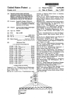
An Antenna Impedance Meter for the High Frequency
1
2
3
4
5
Transcript
Related documents
Chapter 5. - SMAX Technology Co., Ltd.
Owner`s Manual
DF84 - IMB Soft Starter
Technical - Motorcycle Consumer News
TABLE OF CONTENTS
DF56 - Smar
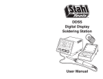
DDSS Manual.indd
Manual 80m version August 8. 2005
Illlllll?l?l?llllllllllllll
0312 antenna analyzers
to read the User Manual
West Mountain Radio RIGrunner 4005i Specifications
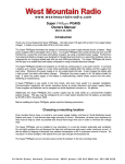
www.westmountainradio.com Super PWRgate PG40S Owners Manual
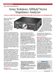
ZMAN ver2.2
1 Introduction
Manual Rev 2.6.5 (pdf 8 MB)
AD9851
Manuel de contrôle
The Chawed Rag-08-2013
Open Access - Lund University Publications
West Mountain Radio Battery Box Specifications
SMALLEST POWERLESS™ SMART DPM MODEL 6K