1
An Antenna Impedance Meter for
the High Frequency Bands
When SWR isn’t enough — here’s a tool that you can build.
Bob Clunn, W5BIG
An
SWR meter is a very useful
instrument and in many situations provides all the information needed to check an antenna. However,
an impedance meter provides a much more
detailed picture of the antenna parameters.
There are several such instruments on the
market with prices in the range to appeal
to hams.1 These typically have broadband
inputs and use diode detectors. The broadband input is subject to incorrect reading due
to strong signals, such as broadcast radio stations, even when the frequencies of these signals are a long way from the test frequency.
The diode detectors are subject to nonlinearity error at low signal levels, so their dynamic
range may be limited.
Design Goal
My goal was to design an instrument
for accurately measuring impedance, with
magnitude and phase, so that all the desired
parameters of an antenna can be determined and displayed in a graphical format.
The resulting antenna impedance meter
(AIM430) measures RF voltage and current
and uses these values to calculate complex
impedance and other parameters of interest. The AIM430 provides a detailed look at
the antenna system. Formulas in the design
books become more meaningful when you
can quickly see how the real and imaginary
parts of the impedance vary with frequency.
The AIM430 continuously covers the
frequency range of 500 kHz to 32 MHz and
operates in conjunction with a PC, which
allows easy control through a graphical user
interface. It can also be battery powered and
connected to a laptop computer for completely portable operation.
required frequencies are generated by two
AD9851 direct digital synthesizer (DDS) integrated circuits made by Analog Devices. One
DDS operates at the specified test frequency
and the other is programmed to operate 1 kHz
above it. These are both driven by a crystalcontrolled oscillator running at 20 MHz. The
DDS chips internally multiply this clock by a
factor of six, so the effective clock rate seen by
the DDS is 120 MHz. In general, the DDS can
be used to produce an output up to about onethird of its clock frequency.2 A block diagram
of the AIM430 is shown in Figure 1.
The output of each DDS is followed by a
low pass filter with a cutoff frequency of 45
MHz. These filters remove the spurious high
frequency components that appear in the output. The DDS generates many frequency components in addition to the one that is desired.
For example, if the DDS is programmed for 32
MHz, there is a strong signal at the clock frequency minus 32 MHz, in this case 120 – 32 or
88 MHz. Therefore, to get good attenuation at
88 MHz and beyond, the DDS low pass filter
cutoff is set at 45 MHz. The filter attenuation
is greater than 60 dB above 88 MHz.
After the DDS output is filtered, it is used
directly to provide the stimulus signal for the
impedance measurement. There is no buffer
amplifier. This eliminates the harmonic distortion of an amplifier and keeps the output
signal amplitude low to reduce the interference to nearby radio receivers. The maximum
output power is less than 50 µW.
The output amplitude of the DDS goes
down slightly as the frequency goes up. The
variation over the entire operating range of the
analyzer is only about 3 dB. This is no problem
since we are using the ratio of two RF signals
to calculate impedance and the amplitude of
the stimulus cancels out in this ratio.
To calculate impedance, we need two
values, voltage and current. Both the magnitude and the phase are measured. These two
parameters are sensed using 1% resistors.
(There are no transformers in the AIM430.)
The voltage across one resistor is proportional
to the voltage being applied to the circuit
under test and the voltage across another
resistor is proportional to the current flowing
into the circuit connected to the analyzer’s
test port. The ratio of these two voltages corresponds to the impedance we want to measure. Figure 2 shows the voltage and current
waveforms.
In Figure 3 there are two mixers, one for
Basic Operation
The AIM430 uses two frequency sources
that are heterodyned to produce a low frequency signal in the audio range that can be
easily amplified, filtered and analyzed. The
1Notes
28
appear on page 32.
November 2006
Figure 1 — Block diagram of AIM430 antenna analyzer.
Reprinted with permission; copyright ARRL
Figure 2 — Voltage and current waveforms
with complex load.
Figure 3 — Schematic of the voltage and current sensing circuits. Two mixers are used
to convert the load current and load voltage to the audio range (typically 1 kHz).
Figure 4 — One of the two 1 kHz
differential amplifiers and band-pass filters.
sensing the current flowing into the load and
the other for sensing the voltage applied to
the load. FDRV is the programmed test signal
from one of the DDSs. This is the stimulus
signal for the load under test. FREF is the output of the other DDS, which is 1 kHz higher
in frequency than FDRV. This second DDS
is the local oscillator. The SA612 has differential inputs, which make it very handy to
directly measure the voltage across a current
sensing resistor. Therefore, we don’t have to
use transformer coupling.
The output impedance of the SA612 is
about 1500 Ω. A 0.01 µF capacitor to ground
filters out the high frequency component (the
sum of the input and local oscillator), leaving
the 1 kHz difference signal. The differential
outputs of the mixers are connected to opamps through dc blocking capacitors. These
capacitors also provide attenuation at low
frequencies.
Figure 3 shows the input protection circuit
of the AIM430. An isolation relay is open
except when a measurement is in progress. A
gas discharge tube (GDT) protects the input
against high voltage due to static charge on
the antenna.
One of the op amp circuits is shown in
Figure 4. There are two poles of high frequency
attenuation including the R-C filter at the out-
put of the mixer. A third pole is provided by a ter because the program is computationsample-hold circuit later in the analog signal ally intensive. I’ve run it successfully on a
processing chain. The frequency response of 300 MHz laptop using Windows 95. The
the signal path peaks at 1 kHz and is 60 dB program doesn’t require an installation prodown at 100 kHz. The op-amps provide filter- cedure; just click on the .exe file and it runs.
ing and also convert the differential signal to a It can be copied to a hard drive or run directly
single ended signal for input to the analog to from a floppy or a CD.
digital converter (ADC). Since the desired signal is always 1 kHz, we do not have to worry Data Analysis
about variations in the amplitude and phase
The two sets of digital data from the voltresponse of the low pass filters.
age and current sensors are analyzed using the
Identical mixer and amplifier circuits are discrete Fourier transform. This produces the
used for both the voltage and current sensing amplitude and phase of the 1 kHz fundamental
paths. Any small differences in the gain and signal and cancels out any dc component due
phase shift of these two paths are taken care of to offsets in the operational amplifiers. The
by the calibration process, which will be dis- magnitude of the load impedance is the voltcussed later. After the RF signals are converted age amplitude divided by the current amplito the audio range, it is much easier to measure tude. The phase angle of the impedance is the
their amplitude and phase. This is done by difference in the phase angles of the voltage
digitizing the two signals with a 12-bit ADC and current. Knowing these two parameters,
that is contained in the Texas Instruments we can calculate the equivalent resistance and
MSP430F149 microprocessor. This micropro- reactance of the load impedance:
cessor runs at 7 MHz and the ADC samples
R = Resistance = Impedance_Magnitude
are precisely timed by its internal clock. Both × cosine(phase_angle)
the current and the voltage channels are samX = Reactance = Impedance_Magnitude ×
pled with 16 samples per cycle.
sine(phase_angle)
The raw data is sent to a PC through the
The external load resistance is found by
RS232 serial port (an RS232/USB converter subtracting the internal 100.6 Ω series resiscan also be used). The PC calculates the tance (R21 + R22 shown in Figure 3) from the
impedance and all the other desired param- calculated resistance. The equivalent series
eters. The PC then graphically displays a circuit is Z = R + jX, where j is the square root
detailed view of the parameters as the fre- of –1. The equivalent parallel circuit is also
quency range is scanned.
calculated and displayed in the data window as
The software has been used with Windows the cursor moves along the frequency axis.
95, 98, 2000 and XP. There is no definite
Resistance is always a positive number.
speed requirement, although faster is bet- Reactance can be positive or negative. Positive
November 2006
29
reactance is associated with inductance and
negative reactance with capacitance. The true
sign of the phase angle is determined by the
data processing routine, so capacitive reactance and inductive reactance can be distinguished without ambiguity. As can be seen
from the scan pictures, the phase changes rapidly as it passes through zero. Critical points
in the plot, such as maximum or minimum
impedances, can be located more accurately on
the frequency axis using phase rather than by
looking only at the impedance magnitude.
at the antenna back toward the transmitter.
(Its magnitude is also equal to the square
root of the ratio of reflected power to incident power.) If there is no reflection (i.e.,
the reflection coefficient is zero) then all the
power from the transmitter is absorbed by the
antenna, which is usually the desired case. If
the transmission line is open at the antenna
(perhaps due to a broken wire), all the power
arriving at the break point is reflected back
toward the transmitter, none is radiated, so
the reflection coefficient has its maximum
value of unity. If the transmission line is open,
the reflection coefficient is plus one; if the
Standing Wave Ratio
line is shorted, the reflection coefficient is
SWR is probably the antenna’s most minus one.
interesting parameter. This is calculated by
first determining a parameter called reflec- Reflection_coefficient = ρ
= (ZL – Z0) / (ZL + Z0)
tion coefficient. When a signal travels down a
transmission line with a characteristic imped- where
ZL = Impedance of the load
ance of Z0 and arrives at the antenna with a
Z0 = Impedance of the transmission line.
different impedance, some of the signal is
reflected back toward the transmitter. This
ZL is a complex number; therefore, ρ is, in
reflection occurs even if the transmission line general, a complex number with a magnitude
is of the highest quality and the antenna is a between 0 and 1 and a phase angle in the
perfect radiator. The reflection coefficient is range ±90°.
the fraction of the voltage that is reflected
Since the reactive component of Z0 is
Figure 5 —
Scan of 28 foot
unterminated coax.
Figure 6 — Smith chart of 28 foot unterminated coax.
30
November 2006
usually very small, it is often ignored and
Z0 is considered to be a real number, such as
“50 Ω” or “75 Ω.” The value of Z0 can be
entered from the program’s main menu, so
the SWR can be calculated for any value of
transmission line impedance.
For the SWR calculation let U equal the
magnitude of ρ.
U will be in the range of 0 to 1.
SWR = (1+U) / (1–U)
Note the SWR only depends on the magnitude of ρ, so it is not a complex number. If
ρ is zero (no reflection), the SWR is 1.0:1.
Since a term 1–U appears in the denominator,
the SWR can be very large when the transmission line is badly matched to the antenna
and the magnitude of the reflection coefficient, U, is almost equal to one.
Applications
The analyzer’s test conditions are specified by entries on the PC. These include scan
start/stop frequencies, frequency increment
between data points and display scale factors.
There is also a provision to enter the nominal
transmission line impedance so the SWR can
be calculated for any value. After the scan is
complete, the mouse can be used to move a
cursor along the frequency scale to display
the numeric values of several parameters
including SWR, impedance magnitude and
phase, equivalent series circuit and equivalent
parallel circuit.
The full-scale ranges for measurements
are:
SWR up to 100:1
Impedance magnitude 1 Ω to 10 kΩ.
Phase angle –90 to +90°.
Frequency scan 500 kHz to 32 MHz.
•
•
•
•
Figure 5 shows the scan of a piece of RG58 coax that is open at the far end. The coax
is 28 feet long. The frequencies at which the
phase angle crosses the axis are called “resonant frequencies” and are listed across the top
of the graph. In this case, the first frequency
corresponds to the 1⁄4 λ of the coax. The second value is the 1⁄2 λ frequency. Because of
loss in the cable, the maximum impedance
at the 1⁄2 λ frequency (11.681 MHz) is only
about 1200 Ω at the input end of the coax, not
infinity. At the frequency corresponding to
a 1 λ, 23.467 MHz, the impedance is about
800 Ω because of increased loss at the higher
frequency. The 1 λ and 1⁄2 λ frequencies are not
exactly in a 2:1 ratio because the velocity of
propagation varies slightly with frequency.
Notice the way in which the phase angle
(violet trace) changes rapidly at 5.765 and
17.532 MHz even though the magnitude of
the impedance is changing slowly. Finding
the phase angle zero crossing makes the location of the 1⁄4 λ frequencies more accurate
than relying on the magnitude of the impedance. The cursor is the light colored vertical
line at 11.697 MHz and the data displayed
Figure 7 — Scan of 28 feet of RG-58 coax with a 243 Ω resistor
termination.
in the window on the right side of Figure 5
corresponds to this frequency. Rs and Xs are
the series circuit values. Rp and Xp are the
parallel circuit values.
Figure 6 shows a Smith chart of the data
from the scan in Figure 5. The small dot at
about the 1 o’clock position is a marker that
Figure 8 — Scan of Figure 7 configuration referred to antenna
terminals.
moves along the Smith chart as the cursor cable loss increases with frequency.
moves along the frequency axis. In this picture the cursor is at 9.515 MHz. The equiva- Reference Transformation
lent series and parallel circuit values are
Sometimes it is desirable to know the
shown on the Smith chart along with the real impedance directly at the antenna terminals.
and imaginary parts of the reflection coef- After a calibration phase during which the
ficient. The trace spirals inward because the properties (length and loss) of the cable are
determined at each measurement frequency,
measurements made at the transmitter end
of the line can be transformed to the antenna
terminals. This is done in real time during the
scan and the displayed data is very close to
what would be measured if the analyzer were
Figure 9 — Two
actually mounted at the antenna.
scans of a series
The calibration is done by disconnecting
L–C tuned circuit
termination. The
the far end of the transmission line from the
first is with the
antenna and then scanning the cable input
circuit connected
impedance with two different resistive termidirectly to the
nations. One terminating resistor is typically
AIM430, the second
is referenced to the
in the range of 20 to 100 Ω and the other can
end of the coax. In
be in the range of 1 kΩ to 2 kΩ. The resisthe ideal case, they
tor values are not critical, as long as they are
would be identical.
accurately measured with a digital ohmmeter. When the transmission line calibration
is performed, the exact resistor values are
entered in the program via dialog boxes. The
terminating resistors can be low power film
devices since they don’t have to handle the
transmitter power. After the cable calibration
is finished, the data are saved to disk so they
can be recalled anytime later.
Using the Impedance
Transformation Feature
(A)
(B)
Figure 10 — Scans with and without interfering signal. At A, a scan without interference.
The SWR reading (red trace) is 3:1 in this example. At B, a scan with a CW interference
level of +63 dB over S-9 injected directly into the input.
Figure 7 shows a conventional scan with
the 243 Ω resistor at the end of 28 feet of RG58 coax. The green trace is the magnitude
of the measured impedance. As expected,
the value varies over a wide range as a function of frequency. At the 1⁄2 λ frequency,
11.621 MHz, the indicated impedance is
close to 243 Ω because the same impedance
is seen at both ends of a half-wave line.
Now we click SETUP and REF TO
ANTENNA. The legend REF TO ANTENNA is
November 2006
31
Figure 12 — There
are two PC boards
sandwiched together
with 0.1×0.1 inch
connectors. The top
board contains all
the RF circuitry and
the bottom board has
the microprocessor
and electronic power
switch. The 3.3 V
regulator is mounted
on the rear panel that
acts as a heat sink.
Figure 11 — The enclosure is 5×5×2
inches, which leaves room inside for an
optional battery pack. The dc current
required is about 150 mA while taking
a measurement and 30 mA if idle. After
10 minutes of inactivity, the dc power is
turned off automatically. Two LEDs on the
front panel indicate POWER ON (green) and
TEST IN PROGRESS (red).
ers. The output into a 50 Ω load is about Acknowledgments
35 mVrms. The amplitude is not precisely caliI would like to thank Dave Russell, W2DMR,
brated but the variation over any of the ham Danny Richardson, K6MHE, and Paul Collins,
displayed in red at the top of the graph while bands is less than 0.5 dB. The frequency can ZL3PTP, for evaluating the AIM and providing
this feature is enabled. The resistor (243 Ω) be set in 1 Hz increments and it can be cali- suggestions that greatly enhanced the program.
and the cable are the same as used in the brated against WWV.
Thanks also to Bill Cantwell, WB5SLX, and
previous graph. The Zmag plot (shown in
Forest Cummings, W5LQU, for their proofgreen) is relatively flat across the frequency Calibration
reading and encouragement.
range. The measured resistance now varies
The AIM430 is calibrated by measuring
only from 243 to 248 Ω, a range of 2%. The the residual capacitance and inductance in its Notes
phase angle and the reactive component are output circuit. The phase shift and amplitude 1J.Hallas, W1ZR, “Product Review — A Look at
Some High-End Antenna Analyzers,” QST,
nearly zero.
differences in the voltage and current amplifiMay 2005, pp 65-69.
Figure 9 shows that the transformation ers are also measured. This calibration data is 2Direct digital synthesizers, theory of
operation — www.analog.com/library/
also works quite well with a complex load then used to compensate each reading. Stray
circuit. A series L-C tuned circuit was used capacitance and inductance associated with 3 analogDialogue/archives/38-08/dds.pdf.
AIM430 User Manual and demonstration profor the load. For the first scan, it was con- an external test fixture, if used, are also taken
gram — w5big.home.comcast.net/antenna
_analyzer.htm.
nected directly to the BNC connector on the into account by this procedure.
4Data sheet for AD9851 DDS — w5big.home.
AIM430. Then it was rescanned with the load
Calibration is performed by using a short
comcast.net/AD9851.pdf.
at the end of 28 feet of coax. The impedance circuit and an open circuit. First, a short cir- 5Data sheet for SA612 mixer — w5big.home.
and reactance curves almost coincide; it’s cuit is connected to the analyzer and several
comcast.net/SA612.pdf.
hard to see the difference between them on measurements are taken. Then the short is 6Data sheet for MSP430F149 microprocessor — focus.ti.com/docs/prod/folders/
the graph. There is only a small difference in removed and the open circuit properties are
print/msp430f149.html.
7
the two phase-angle traces shown in violet.
measured. This data is saved in a file that is
Schematic and printed circuit board design
software — www.expresspcb.com.
automatically loaded each time the program
Interference Rejection
is run. The whole calibration process takes
The band pass circuits in the AIM430 only a few seconds. Since the analyzer does
Bob Clunn, W5BIG, received his Novice
help to reject interfering signals that are more not have any internal adjustments (no pots or license in 1956 while in junior high and
than about 100 kHz from the desired test trim caps), the calibration is very stable. It his general license soon after. During high
frequency. Figure 10 shows the result with only needs to be done when the external test school he was very active on 40 and 20 meter
CW. During this time he made the decision
and without an interfering signal that has an fixture or cable adapter is changed.
to study electrical engineering in college.
amplitude of +63 dB over S-9. The disturBob
received his BS degree in electrical engiConstruction
bance of the reading is confined to an interval
of about ±100 kHz.
The microprocessor is initially pro- neering from Rice University in 1965 and his
grammed through a 14-pin JTAG interface. MS from Southern Methodist University in 1969.
Additional Applications
Subsequently, the program can be updated He was employed at Texas Instruments in Dallas
from 1963 until 1991. His work there involved
In addition to measuring antennas, the through the standard RS-232 interface.
the design of computer controlled test equipment
AIM430 can be used to measure discrete
for transistors and integrated circuits. From 1991
Conclusions
components, such as resistors, capacitors and
to the present he has been working as a consulinductors. It is particularly interesting to see
The operation of an affordable vector tant for several companies in the fields of elechow the component value varies as a function impedance meter for measuring antennas in tronic circuit design and machine vision.
of frequency. Inductors with metal cores are the high frequency range has been presented.
In 2002, Bob renewed his interest in ham
often very frequency sensitive. It can also Using state-of-the-art components for signal radio and obtained his Amateur Extra class
be used for adjusting tuned circuits, such as generation and analysis, the AIM430 provides license. Soon afterward he got interested in
traps, and for measuring the parameters of a high level of accuracy and wide dynamic equipment to evaluate antennas and began
quartz crystals and other resonator devices.
range for complex impedance measurements. the design of this antenna analyzer. He can be
The output signal from the analyzer can The unit is also quite useful for measuring dis- reached at 509 Carleton Dr, Richardson, TX
be used as a test signal for checking receiv- crete components and tuned circuits.
75081 or at [email protected].
32
November 2006