Download Redalyc.Syntactic transformation rules under P

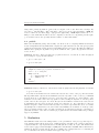
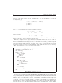
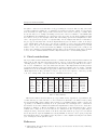
Inteligencia Artificial. Revista Iberoamericana
de Inteligencia Artificial
ISSN: 1137-3601
[email protected]
Asociación Española para la Inteligencia
Artificial
España
Pascucci, Simone; López Fernández, Alejandra
Syntactic transformation rules under P-Stable semantics: theory and implementation
Inteligencia Artificial. Revista Iberoamericana de Inteligencia Artificial, vol. 13, núm. 41, 2009, pp. 2137
Asociación Española para la Inteligencia Artificial
Valencia, España
Available in: http://www.redalyc.org/articulo.oa?id=92513168003
How to cite
Complete issue
More information about this article
Journal's homepage in redalyc.org
Scientific Information System
Network of Scientific Journals from Latin America, the Caribbean, Spain and Portugal
Non-profit academic project, developed under the open access initiative
Inteligencia Artificial 41(2009), 21-37
doi: 10.4114/ia.v13i41.1028
INTELIGENCIA ARTIFICIAL
http://erevista.aepia.org/
Syntactic transformation rules under P-Stable
semantics: theory and implementation
Simone Pascucci1 , Alejandra López Fernández2
1
Universitá di Roma “La Sapienza”
Via Salaria, 113
Roma, 00184 (Italy)
[email protected]
2
Computational Linguistics Department
Saarland University
Saarbruecken (Germany)
[email protected]
AbstractWe study the simplification of normal logic programs under the P-Stable semantics, with respect to the
notions of equivalence, using many of the transformation rules found in literature in the context of Answer Set
Programming (ASP). A schema for the implementation of P-Stable semantics is provided using two well known
open source tools: Lparse and Minisat. Also, a prototype written in Java of a tool based on this schema is
presented. We extend the work of Fernández [4] including a simplification routine in the post-parsing phase.
Keywords: Non Monotonic Reasoning, Logical Programming, P-Stable Semantics, Syntactic Trasformation.
1
Introduction
The P-Stable semantics lies in the context of Non-Monotonic reasoning and was defined by means of
a fixed-point operator in terms of classical logic [2]. Many other semantics, defined in terms of weak
completion by a large class of logics, were proved to be equivalent to the P-Stable semantics for normal
logic programs [2]. The well-known Stable semantics (Gelfond and Lifschitz, 1998 [18]) has been proved
to be related to the P-Stable semantics, in fact given a normal logic program P , let M M (P ), S(P ) and
P S(P ) denote respectively the set of all the minimal models of P , the set of all the Stable models of P
and the set of all the P-Stable models of P , we have that S(P ) ⊆ P S(P ) ⊆ M M (P ) [2]. For example,
let P be the following normal program
a ← not b
we have M M (P ) = {{a}, {b}}, P S(P ) = {{a}}, S(P ) = {{a}}. Such characterization guided us in
the development of the implementation schema, giving the hint on how to generate a procedure that
could find the P-Stable models of a given normal program. In the context of finding quick procedures
to compute P-Stable models we study in this paper many of the syntactic transformation rules found
in the context of ASP [8, 9], giving results about their equivalence preserving properties under P-Stable
semantics. Moreover, many syntactic transformations are not only valuable in terms of a fast computation
of models, but they also provide a way to simplify programs that are used as base for larger ones, this
kind of transformations are said to preserve strong equivalence (see next sections). It remains to mention
ISSN: 1988-3064(on-line)
c
°AEPIA
and the authors
22
Inteligencia Artificial 41(2009)
that there are applications, such as in the theory of argumentation, in which a behavior closer to classical
logic is needed [17]. In such cases the P-Stable semantics provides a solution since it can be expressed
using only classical logic [17].
We present a schema for the implementation of a tool that computes the P-Stable models of a given
normal logic program extending the work of Fernández [4] with the inclusion of a simplification routine
in the post-parsing phase. A prototype written in Java implementing such a schema can be obtained at
http://cxjepa.googlepages.com.
This paper is structured in the following way. In the Section 2 we resume the basic theory underlying the
P-Stable semantics. In Section 3 we give the definitions and properties of the syntactic transformations
that can be applied to normal logic programs. In Section 4 we expose such a schema presenting also a
small prototype written in Java. Finally, in Section 5 we make our final considerations giving hints and
directions about future works and improvements to the tool.
2
Basic Theory
In this section, the notation used in the rest of this paper as well as some fundamental results about
P-Stable semantics are presented.
2.1
The Framework
Most of the definitions and results given here are taken “as they are” from the works of Baral [1] and
Osorio et al. [2]. A more interested reader can refer to these documents to have a deeper vision of the
subject. The language which we are dealing with is known to be a declarative one, meaning, informally,
that we are able to express what the solution of the problem should look like instead of giving a procedure
that says how to compute it. For both lexical and syntactic characteristics refer to Lparse user manual,
[5], and Baral [1] Section 1.2. We give now the definition of the main constituents of our language:
Definition 2.1. A term is defined as follows:
1. A variable is a term.
2. A constant is a term.
An atom is of the form p(t1 , . . . , tn ) where p is a predicate symbol and every ti is a term, for i = 1 . . . n.
A naf-literal is either an atom or an atom proceeded by the symbol not .
A term is said to be ground if no variable occurs in it. Given an atom p(t1 , . . . , tn ), if every ti is
ground, for i = 1 . . . n, then the atom is said to be ground.
Remark 2.2. In this paper the so called “classical negation/strong negation” of ASP is not considered.
Definition 2.3. A normal logic program is a collection of rules, or clauses, of the form:
a0 ← a1 , . . . , am , not am+1 , . . . , not am+n .
where each ai is an atom.
The parts on the left and on the right of ’←’ are called the head and the body of the rule, respectively.
A rule with an empty body is called a fact. Given a rule r, we define the sets H(r) = {a0 }, B + (r) =
{a1 , . . . , am }, B − (r) = {am+1 , . . . , am+n }, B(r) = B + (r) ∪ B − (r).
Note that a fact (a0 ← .) is often denoted by only his head (a0 .). The notation just introduced
follows the tradition of logic programming to define a propositional language built from an enumerable
set L of atoms, the binary connectives ∧ (conjunction) and → (implication) and the unary connective ¬
(negation). Given a set of atoms M = {a1 , . . . , am }, we define ¬M = {¬a1 , . . . , ¬am }. In this paper a
rule r as in Definition 2.3 stands for a formula of the language of the type
^¡
¢
B + (r) ∪ ¬B − (r) → H(r)
Inteligencia Artificial 41(2009)
23
while a normal program is just a set of formulas or a theory.
The Herbrand universe of a logic program is the set of all ground terms that can be constructed using
constants in that program. The Herbrand base of a logic program is the set of all ground atoms that
can be constructed using the predicates of the program and the terms of the Herbrand universe. An
instance of an atom, a literal or a rule is constructed by replacing all variables in it by ground terms.
The Herbrand instantiation is the set of all ground instances of the rules that may be constructed using
terms in the Herbrand universe of P . The signature of a ground program P , notation LP , is the set of
all ground atoms that appear in P .
The concepts related to the grounding process bypass the scope of this paper and for that reason are
omitted. In the rest of the paper we are going only to consider ground finite programs.
2.2
Semantics
Before talking about the P-Stable semantics, we briefly resume some fundamental concepts of classical
logic which are strictly related to the former one. For an introduction about terminology and concepts of
classical logic refer for example to Ben-Ari [3]. We consider a logic X as a set of formulas that is closed
under modus ponens and is closed under substitution. The elements of a logic X are called theorems and
the notation `X A is used to state that the formula A is a theorem of X.
Definition 2.4 (model). A set of formulas U = {A1 , . . . , An } is satisfiable iff there exists an interpretation
v such that v(A1 ) = . . . = v(An ) = T , where T stands for the constant true. The satisfying interpretation
is called a model of U .
Note that from this point on a model will be referred as the set of the atoms that evaluate true in the
interpretation.
Definition 2.5 (minimal model). A set of atoms M is a minimal model of a program P (or set of formulas
U , as previously said) if M is a classical model of P and is minimal (with respect to set inclusion) among
other classical models of P .
Definition 2.6 (logical consequence). Let U be a set of formulas, A be a formula and X be any logic.
A is a logical consequence of U in the logic X iff `X (F1 ∧ . . . ∧ Fn ) → A for some formulas Fi ∈ U .
Notation: U `X A.
Remark 2.7. Following the notation of Osorio et al. [2], we extend the above definition including the
notion of logical implication between two theories T and U in any logic X using T `X U to state the fact
that T `X F for all formulas F ∈ U . If M is a set of atoms we write T °X M when T `X M and M is
a classical two-valued model of T .
The definition of a P-Stable model is now given with some fundamental results that have been used
in the implementation schema (refer to the work of Osorio [2] Section 4.3).
Definition 2.8 (Reduction). Let P be a normal program and M a set of atoms. We define RED(P,M)
as the following set of clauses
{H(r) ← B + (r), not (B− (r) ∩ M )|r ∈ P }
Definition 2.9 (P-Stable model). Let P be a normal program, and M a set of atoms. We say that M
is a P-Stable model of P if RED(P, M ) °C M .
Note that the subscript C denotes the fact that we are talking about classical logic semantics.
Example 2.10. Let P be the program:
P :
a ← not b.
(1)
b ← not a.
(2)
p ← not p.
p ← a.
(3)
(4)
24
Inteligencia Artificial 41(2009)
then, given the set of atoms M = {p, a}, we have
RED(P, M ) :
a.
b ← not a.
p ← not p.
p ← a.
(5)
(6)
(7)
(8)
M is a P-Stable model of P . To see that, first note that M is a model of RED(P, M ). Moreover,
RED(P, M ) `C M because does not exist any other model M 0 of RED(P, M ) such that M * M 0 . This
follows from the syntactic structure of rules (5) and (8).
To conclude the section, we reproduce a theorem that state the relation between minimal and P-Stable
models.
Theorem 2.11 (Osorio et al. [2]). Let P be any theory, and M a set of atoms. If M is a P-Stable model
of P then M is a minimal model of P .
Example 2.12. Let P be the normal logic program as defined in Example 2.10, M = {p, a} and
M 0 = {p, a, b}. We have that RED(P, M 0 ) = RED(P, M ) \ {a.} ∪ {a ← not b.} = P . M , which is a
P-Stable model of P , is also a minimal model of P . M 0 is a model (not minimal) of P , then it is also a
model of RED(P, M 0 ) but we have that RED(P, M 0 ) 0C M 0 . So, M 0 is not a P-Stable model of P .
3
Transformations rules
In this section we study some transformations already defined in logic programming literature, giving
results about their applicability to normal logic programs under P-Stable semantics. We know from Osorio
et al. [9] that SUB, TAUT, RED− and SUC preserves strong equivalence under Stable semantics, while
RED+ and GPPE preserves equivalence only. We briefly resume some definitions and properties of logic
programs under P-Stable semantics such as the notions of equivalence and their relation with the logic
G03 .
Definition 3.1. Let P, P 0 be two normal logic programs. We say that:
(a) P is equivalent to P 0 , notation P ≡e P 0 , if P and P 0 have the same set of P-Stable models.
(b) P is uniformly equivalent to P 0 , notation P ≡u P 0 , if for any set of atoms M , P ∪ M and P 0 ∪ M
are equivalent.
(c) P is strongly equivalent to P 0 , notation P ≡s P 0 , if for any normal logic program P 00 , P ∪ P 00 and
P 0 ∪ P 00 are equivalent.
Note that from the definition follows that (c) ⇒ (b) ⇒ (a). The G03 -logic is a logic system which has
been used to introduce a new semantics for non-monotonic reasoning and which has been proved to be
equivalent to the P-Stable model semantics for normal program [2]. One of the main results of Osorio et
al. [11] is that for any two arbitrary logic programs P and P 0 if P ≡G03 P 0 then P and P 0 are strongly
equivalent under P-Stable semantics. For an axiomatization of G03 refer to the work of Osorio [15]. Basic
transformation rules are defined in terms of binary relations on the set P of all programs [9]. We consider
a basic transformation rule B as a syntactic operator B : P → P which is identified with the identity
operator when the conditions for its applicability are not satisfied.
3.1
Transformation rules preserving equivalence
Definition 3.2 (sub-implication). A rule r0 is a sub-implication of another rule r such that r 6= r0 ,
symbolically r J r0 , iff H(r) = H(r0 ), B + (r) ⊆ B + (r0 ), B − (r) ⊆ B − (r0 ).
Inteligencia Artificial 41(2009)
25
Note that SUB is also known in the literature of automated reasoning and artificial intelligence as
subsumption.
Definition 3.3 (SUB). Let P be a normal logic program and r, r0 ∈ P such that r J r0 . Then, replace
P by P \ {r0 }.
Example 3.4. Let P be the program:
P :
a ← b, not b.
(1)
a ← b, e, not b, not a.
(2)
we can apply SUB to clauses (1) and (2) to obtain the following reduced program P 0 :
P0 :
a ← b, not b.
(1)
SUB preserves strong equivalence also under P-Stable semantics, as shown in the next proposition.
Proposition 3.5. Let P be a normal logic program. Then P ≡s SU B(P ).
Proof. Let P \ {r0 } be denoted by P 0 , B + (r0 ) \ B + (r) by Q+ , B + (r0 ) \ B + (r) by Q− . We have to show
that (i) for all clauses F in P , P 0 `G0 F , and (ii) for all clauses G in P 0 , P `G0 G. (i) The result follows
3
V3
directly from the proof for P 0 `G0 (B + (r0 ) ∪ ¬ B − (r0 )) → H(r0 ):
3
P 0 ,Q+ ,¬ Q−
^
(B + (r) ∪ ¬ B − (r)) → H(r)
` G0
3
Asmpt (1)
P 0 ,Q+
` G0
3
^
+ 0
−
( (B (r ) ∪ ¬ B (r)) → H(r)) Ded 1 (2)
P0
` G0
3
^
( (B + (r0 ) ∪ ¬ B − (r0 )) → H(r)) Ded 2 (3)
(ii) For all G in P 0 we have that G is also in P .
Definition 3.6 (TAUT). Let P be a normal logic program and r ∈ P a rule such that H(r) ∈ B + (r).
Then, replace P by P \ {r}.
Example 3.7. Let P be the program:
P : a ← a, not b.
b ← not a.
(1)
(2)
we can apply TAUT to clause (1) to obtain the following reduced program P 0 :
P 0 : b ← not a.
(1)
Proposition 3.8. Let P be a normal logic program. Then, P ≡s T AU T (P ).
Proof. The proof is similar to the one of Proposition 3.5 considering that `G0 a → a.
3
0
Definition 3.9 (SUC). Let P be a normal logic program, r, r ∈ P such that H(r0 ) ∈ B + (r), B(r0 ) = ∅.
Then, replace P by P \ {r} ∪ {r00 }, where r00 is
H(r) ← (B + (r) \ H(r0 )), not B − (r).
The transformation SUC is also well known in literature as unit propagation.
26
Inteligencia Artificial 41(2009)
Example 3.10. Let P be the program:
P : c ← not b.
b ← a, not c.
a.
(1)
(2)
(3)
we can apply SUC to clause (2) to obtain the following reduced program P 0 :
P 0 : c ← not b.
b ← not c.
a.
(1)
(2)
(3)
Proposition 3.11. Let P be a normal logic program. Then, P ≡s SU C(P ).
Proof. (P `G0 {P \ {r}} ∪ {r00 }).
3
P `G0
^
(B(r) ∪ {a}) → H(r)
Asmpt
(1)
P `G0 a
Asmpt
(2)
P `G0
Equiv 6
(3)
MP 7,8
(4)
3
3
3
P `G0
3
^
a → ( (B(r)) → H(r))
^
(B(r)) → H(r)
({P \ {r}} ∪ {r00 } `G0 P ). Easy derivation using the axiom a → (b → a) and the equivalence (a → (b →
3
c)) → (a ∧ b → c).
The notion of s-implication has been given from Wang and Zhou in [10] for disjunctive normal programs. The analogous version for normal logic program is given in the next definition.
Definition 3.12 (s-implication). A rule r0 is an s-implication of another rule r such that r 6= r0 ,
symbolically r C r0 , iff there exists an atom a ∈ B − (r0 ) such that
(i) H(r) = {a}
(ii) B − (r) ⊆ B − (r0 ) \ {a}
(iii) B + (r) ⊆ B + (r0 )
Definition 3.13 (SS-IMP). Let P be a normal logic program, r, r0 , r00 ∈ P such that r C r0 , H(r) = a as
defined in point (i) of Definition 3.12, H(r00 ) = H(r0 ), B + (r00 ) = {a} and B − (r00 ) = {a}. Then, replace
P by P \ {r0 }.
This is a stronger version of S-IMP, see next subsection, requiring the presence of an extra rule r00
in the program P . Such extra requirement assures that the application of the transformation SS-IMP
preserves strong equivalence under P-Stable semantics.
Example 3.14. We give an example of a normal program P which structure satisfies the applicability
of SS-IMP. Let P be the program of example 3.37. Then, let P 0 = P ∪ {a ← b, not b}. We have that
P 0 and SS-IMP(P) have the same set of P-Stable models {{b, e}, {a}}.
Proposition 3.15. Let P be a normal logic program. Then, P ≡s SS-IMP(P).
Proof. Let P1 be any normal program and M any set of atoms. We start by proving RED(SS-IMP(P)∪P1 ,
M)`C RED(P ∪P1 , M ). Without loss of generality, let us assume B − (r) = B − (r0 )\{a}, B + (r) = B + (r0 )
Inteligencia Artificial 41(2009)
27
and let r00 = RED(r0 , M ), b = H(r0 ), C =
case when a ∈
/ M,
³V
c∈B + (r)
´
³V
´
c ,D=
d∈B − (r 00 ) ¬d . We first consider the
(a ∧ ¬a) → b, (C ∧ D) → a, C ∧ D
(C ∧ D) → a
(a ∧ ¬a) → b, (C ∧ D) → a, C ∧ D
C ∧D
(a ∧ ¬a) → b, (C ∧ D) → a, C ∧ D
` G0
3
Asmpt (10)
` G0
3
Asmpt (11)
` G0
3
a
MP 11, 10 (12)
(a ∧ ¬a) → b, (C ∧ D) → a, C ∧ D
` G0
3
(a ∧ ¬a) → b
(a ∧ ¬a) → b, (C ∧ D) → a, C ∧ D
Asmpt (13)
` G0
3
a → (¬a → b)
Equiv 13 (14)
(a ∧ ¬a) → b, (C ∧ D) → a, C ∧ D
` G0
3
¬a → b
(a ∧ ¬a) → b, (C ∧ D) → a
MP 12, 14 (15)
` G0
(C ∧ D) → (¬a → b)
(a ∧ ¬a) → b, (C ∧ D) → a
Ded. 15 (16)
` G0
(C ∧ D ∧ ¬a) → b
3
3
Equiv 16 (17)
By the definition of C, D and b follows the result. The case when a ∈ M is analogous. For the converse,
just note that every rule of SS-IMP(P) is also in P .
Definition 3.16 (RED+ ). Let P be a normal logic program, r ∈ P a rule and a an atom such that:
(i) a ∈ B − (r),
(ii) @r0 ∈ P such that {a} = H(r0 ).
Then, replace P by P \ {r} ∪ {r00 }, where r00 is H(r) ← B + (r), not (B − (r) \ {a}).
Note that the application of RED+ could generate the conditions satisfying the applicability of some
other transformations. The transformation RED+ does not preserve uniform equivalence as shown in
the next example.
Example 3.17. Let P be the following program,
P : a ← b, e, not b, not c.
(1)
b ← e, not c
(2)
b ← not a.
e ← b, not f.
(3)
(4)
P 0 is the program obtained from P after three applications of RED+ , respectively to rules (1), (2), (4):
P 0 : a ← b, e, not b.
(1)
b← e
b ← not a.
(2)
(3)
e ← b.
(4)
P and P 0 have the same P-Stable models {e, b}, {a}. However, P ∪ {f.} and P 0 ∪ {f.} have different
P-Stable models, respectively {f, b} and {f, b, e}, {f, a}.
28
Inteligencia Artificial 41(2009)
We show now that RED+ preserves equivalence.
Lemma 3.18. Let P be a normal logic program, r ∈ P and a ∈ B(r) such that does not exist a rule
r0 ∈ P : H(r0 ) = {a}. Then, for any set of atoms M , RED(P, M ) 0 a.
Proof. Let
[
M0 =
H(r).
r∈RED(P,M )
The result follows from the considerations that a ∈
/ M 0 and M 0 is a classical model of RED(P, M ).
Proposition 3.19. Let P be a normal logic program. Then, P ≡e RED+ (P ).
Proof. Let M be a P-Stable model of P , r ∈ P and a ∈ B(r) such that does not exist a rule r0 ∈
P : H(r0 ) = a. By Lemma 3.18 we have that a ∈
/ M , then, M is a classical two-valued model also of
RED+ (P ). By Definition 2.8, we have that RED(P, M ) = RED(RED+ (P ), M ). The converse part is
proved by a symmetric argument.
NAF is the abbreviation for Negation as Failure, a transformation that completes the preceding
RED+ :
Definition 3.20 (NAF). Let P be a normal logic program, r ∈ P a rule and a an atom such that:
(i) a ∈ B + (r),
(ii) @r0 ∈ P such that {a} = H(r0 ).
Then, replace P by P \ {r}.
We remark that NAF is also known under the name of Failure [19]. NAF does not preserve uniform
equivalence as shown in the next example.
Example 3.21. Let P be the following program,
P :
a ← not b.
b ← not a.
a ← e.
(1)
(2)
(3)
P 0 is the program obtained from P after three applications of NAF to rule (3):
P 0 : a ← not b.
b ← not a.
(1)
(2)
P and P 0 have the same P-Stable models {b}, {a}. However, P ∪{e.} and P 0 ∪{e.} have different P-Stable
models, respectively {e, a} and {e, b}, {e, a}.
NAF preserves equivalence, as stated in Proposition 3.23.
f °C M iff M is a minimal
Lemma 3.22 ([7]). Let P be any theory and M a set of atoms. P ∪ ¬M
model of P .
Proposition 3.23. Let P be a normal logic program. Then, P ≡e NAF(P).
Proof. Let M2 be a P-Stable model of N AF (P ), r ∈ P and a ∈ B + (r) such that points (i) and (ii)
/ M2 then M2 is a classical model of P . Moreover,
of Definition 3.20 are satisfied. By Lemma 3.18, a ∈
RED(P, M2 ) `C RED(N AF (P ), M2 ), then by transitivity we have RED(P, M2 ) `C M2 . Conversely, let
M1 be a P-Stable model of P . By Definition 2.9, M1 is a classical two valued model of P , being NAF(P)
composed by a subset of the rules present in P we have that M1 is also a classical model of NAF(P). Also,
f1 = LP \M1 , by Theorem 2.11 we have that RED(P, M1 ) `C M1 implies RED(P, M1 )∪¬M
f1 `C M1 .
let M
f
f
f
By Lemma 3.18, a ∈ M1 hence ¬a ∈ RED(P, M1 ) ∪ ¬M1 and ¬a ∈ RED(N AF (P ), M1 ) ∪ ¬M1 . For any
Inteligencia Artificial 41(2009)
29
f1 `C a → b, then RED(N AF (P ), M1 )∪¬M
f1 ≡C RED(P, M1 )∪¬M
f1 .
atom b, RED(N AF (P ), M1 )∪¬M
By Lemma 3.22, M1 is a minimal model of RED(N AF (P ), M1 ), to conclude the proof, let assume by
contradiction that RED(N AF (P ), M1 ) 0C M1 , this implies the existence of a minimal model M2 of
RED(N AF (P ), M1 ) such that M1 ∩ M2 6= M1 . M2 is also a model of RED(P, M1 ) then follows the
contradiction RED(P, M1 ) 0C M1 .
RED− , despite to his name, can be considered the completion of the transformation SUC:
Definition 3.24 (RED− ). Let P be a normal logic program, r, r0 ∈ P such that H(r0 ) ⊆ B − (r),
B(r0 ) = ∅. Then, replace P by P \ {r}.
Example 3.25. Let P be the program:
P :
a ← not b.
b.
(1)
(2)
we can apply RED− to clause (1) to obtain the following reduced program P 0 :
P0 :
b.
(1)
Proposition 3.26. Let P be a normal logic program. Then, P ≡s RED− (P ).
Note that in the proof we cannot use the fact that for any two arbitrary logic programs P and P 0 if
P ≡G03 P 0 then P and P 0 are strongly equivalent under P-Stable semantics. This because given a normal
0
logic program P which satisfies the applicability of RED− , we are not able to prove in G3 a formula
of the type ¬a → b having a between the hypothesis. This would require the presence of the axiom
0
a → (¬a → b) which is one of the axiom we can add to G3 to obtain classical logic [15].
Proof. Let P1 be any normal logic program and r, r0 ∈ P as in Definition 3.24, we must show that P ∪P1 ≡e
RED− (P ) ∪ P1 . Note that a set of atoms M is a model of P ∪ P1 iff M is a model of RED− (P ) ∪ P1 .
This because any such model M must contain H(r0 ) and from this consideration follows that r is satisfied
for any other truth assignment to its remaining atoms. Let consider now RED(RED− (P ), M ) and
RED(P, M ). RED(P, M ) `C RED(RED− (P ), M ) because every formula in RED(RED− (P ), M ) is
also in RED(P, M ). Moreover, we can now use the axiom a → (¬a → b) to easily prove r from the set
of hypothesis RED(RED− (P ), M ). It follows that RED(P, M ) ≡C RED(RED− (P ), M ).
Definition 3.27 (EQUIV). Let P be a normal logic program, r ∈ P a rule such that H(r) ∈ B − (r).
Then, replace P by P \ {r} ∪ {r0 }, where
r0 = H(r) ← B(r), not (B − (r) \ H(r)).
Example 3.28. Let P be the program:
P : a ← not b, not a.
b ← not a.
(1)
(2)
we can apply EQUIV to clause (1) to obtain the following reduced program P 0 :
P 0 : a ← not b.
(1)
b ← not a.
(2)
Proposition 3.29. Let P be a normal logic program, r ∈ P a rule such that H(r) ∈ B − (r). Then,
P ≡s EQU IV (P ).
Proof. It follows from a simple check of the truth tables of connectives in G03 that
^
(B + (r) ∪ ¬ (B − (r))) → H(r) ≡G03
^
(B + (r) ∪ ¬ (B − (r) \ H(r))) → H(r)
30
Inteligencia Artificial 41(2009)
The transformation LOOP has been shown to preserve equivalence under Stable semantics [9]. Let
def inite(P ) denote the definite program obtained from a normal logic program P removing every negative
literal in P . It is a well know result that definite programs have a unique minimal model, refer for example
to the work of Baral [1]. By M M (Def inite(P )) we mean the unique minimal model of Def inite(P ).
Definition 3.30 (LOOP). Let unf (P ) = LP \ M M (Def inite(P )). Then, we define LOOP (P ) = {r ∈
P | B + (r) ∩ unf (P ) = ∅}.
LOOP does not preserve uniform equivalence as shown in the next example, a proof for equivalence
can instead be found in the work of Carballido [16].
Example 3.31. Let P be the program:
P :
a ← e, not b.
(1)
b←
e←
c←
d←
(2)
(3)
(4)
(5)
c.
not b.
d.
c.
we have that M M (Def inite(P )) = {a, e}, unf (P ) = LP \ M M (Def inite(P )) = {a, b, c, d, e} \ {a, e} =
{c, d, b}, LOOP (P ) = {(1), (3)}. P and LOOP (P ) have just one P-Stable model {e, a} but P ∪ {c.} and
LOOP (P ) ∪ {c.} have different P-Stable models, respectively {c, d, b} and {c, e, a}.
3.2
Transformation rules not preserving equivalence
We grouped in this subsection many of the transformation rules found in literature that do not preserve
any type of equivalence, the uninterested reader can safely skip to the next section.
Definition 3.32 (CONTRA). Let P be a normal logic program and r ∈ P such that B + (r) ∩ B − (r) 6= ∅.
Then, replace P by P \ {r}.
CONTRA does not preserve any type of equivalence, as shown in the next example.
Example 3.33.
P : b ← a, not a.
a ← not b.
(1)
(2)
P has two P-Stable models {b}, {a} while P \ {(1)} has just one P-Stable model {a}.
Definition 3.34 (GPPE). Let P be a normal logic program, r ∈ P a rule, a ∈ B + (r) an atom, Ga 6= ∅
0
for Ga = {r0 ∈ P | {a} = H(r0 )}. Then, replace P by P \ {r} ∪ {Ga‡ }, where
0
Ga‡ = {H(r) ← (B + (r) \ {a}) ∪ B + (r0 ),
not (B − (r) ∪ B − (r0 )) | r0 ∈ Ga }.
In P-Stable semantics, GPPE does not preserve equivalence as shown in the next example.
Example 3.35. Let P be the following normal program:
P :
a ← c.
(1)
c ← not b.
(2)
c.
b.
(3)
(4)
Inteligencia Artificial 41(2009)
31
P has one P-Stable model {b, c, a}. After the application of GPPE to rule (1), considering the atom
c ∈ B + ((1)), we obtain the following program P 0
P0 :
a ← not b.
c ← not b.
(1)
(2)
c.
b.
(3)
(4)
which has one P-Stable model {c, b}.
With regard to the weak version of GPPE, WGPPE [8], when applied to normal logic programs
it just adds redundant rules and for that reason is not considered here. We give now the definition of
S-IMP which has been reported to preserve strong equivalence in Stable semantics by Eiter [8].
Definition 3.36 (S-IMP). Let P be a normal logic program and r, r0 ∈ P such that r C r0 . Then,
replace P by P \ {r0 }.
S-IMP does not preserve equivalence as we can see from the next example.
Example 3.37. Let P be the program:
P :
a ← e, not b.
b ← e.
b ← not a.
(1)
(2)
(3)
e ← b.
(4)
P has the two P-Stable models {e, b}, {a}. After the removal of (1) due to the application of S-IMP,
note that (2) C (1), the obtained reduced program has just one P-Stable model {e, b}.
We summarize the results of this section in table 1.
4
Implementation schema
We present the schema directly referring to the prototype written in java we implemented. The source
code is divided into five main packages:
• main.
• dataStructures.
• fileManagement.
• transformations.
• pstable.
We just mention that our prototype makes intensive use of two third party tools, Lparse and Minisat,
respectively available at http://minisat.se and http://www.tcs.hut.fi/Software/smodels. Lparse
is a front-end that generates a variable-free simple logic program. The reason of this choice is that in our
opinion Lparse is the most feature-rich of the different parsers and front ends. We decided to use MiniSat
because of its high efficiency. How reported at MiniSat web page, this SAT solver is the winner of all the
industrial categories of the SAT 2005 competition. The reader interested to the technical background
can refer to their respective user manuals. Also, a brief survey of their usage can be found in [4] and at
the prototype web page (http://cxjepa.googlepages.com).
4.1
main
The main package contains the main method. It implements the tool external interface, which can be used
in any application requiring the computation of the P-Stable models of a given normal logic program.
32
≡e
≡u
≡s
Inteligencia Artificial 41(2009)
SUB
yes
yes
yes
TAUT
yes
yes
yes
SUC
yes
yes
yes
SS-IMP
yes
yes
yes
CONTRA
no
no
no
RED+
yes
no
no
NAF
yes
no
no
RED−
yes
yes
yes
GPPE
no
no
no
EQUIV
yes
yes
yes
LOOP
yes
no
no
Table 1: Summary of the transformation rules. For each notion of equivalence ≡t , for t ∈ {e, u, s}, and
each transformation rule R, it is reported if, given a normal logic program P , P ≡t R(P ).
input : A file f ileN ame containing the description of a normal logic program, a integer n
representing the number of P-Stable models to compute
output: A list of P-Stable models
program ← invokeAndCreateInput(f ileN ame);
if simplification is enabled then simplify(program);
inputM S ← createInputMinisat(program);
modelsList ← calculateModels(program, n, inputM S);
return modelsList;
Algorithm 1: PSI external interface
4.2
dataStructures and fileManagement
The package dataStructures contains the definitions of the two data structures used in the tool, Program
and Rule, plus some general purpose methods. The class Rule is just a container for two variables, an
integer one and an array of integers, respectively the head and the body of the rule to be represented.
It also converts the rule in his CNF form, to be returned in form of an array of integers, as stated by
the logical equivalence A → B ≡ ¬A ∨ B. The class Program represents the program in memory and
contains two private variable, an ArrayList of Rule and a Hashmap where we save the symbol table as
returned from Lparse. Also, it provides many methods that help in the process of simplification. The
package fileManagement is responsible of all the accesses to the file system and to produce the input for
Minisat.
4.3
transformations
All the syntactic transformations we studied in Section 3.1 perform in polynomial time. Following the
schema of the simplify algorithm as depicted in Eiter [8], we implemented a polynomial simplification
routine (Algorithm 2) which applies the following list of syntactic transformation: SUB, SUC, RED− ,
RED+ , NAF, TAUT, EQUIV.
In our implementation the ChangeInfo variable does not operate at level of single rule, instead at
each main iteration it activates the test of a subset of all implemented rules depending on the changes
occurred in the last step. Such changes include the remotion of literals, the introduction of new facts
and the reduction of the set of all the heads. Some transformations, as TAUT and EQUIV, do not
need to be tested more than once and for that reason are activated only in the first iteration. In the
implementation we made use of some data structures created during the parse of the output of Lparse:
the list of facts is maintained in a HashSet which guarantees constant time performances for the basic
operations (add, remove, contains and size) assuming the hash function disperses the elements properly
among the buckets, the list of head is maintained in a HashMap< key, value > where the key is the
integer representing the atom and the value is the number of occurrences of the atom as head (also in this
case the basic operations perform in constant time). Under such assumptions plus the one that a literal
can be removed in constant time from the body of a clause, the step of testing SUC, RED− , RED+ ,
NAF, TAUT, EQUIV has worst-case running time of the order of O(n × m), where n is the number of
rules in the program and m is the average size of the bodies. The transformation SUB, which performs in
quadratic time with a brute-force algorithm, has been implemented making use of two sorting steps. The
first one sorts all the rules depending on the value of the head as assigned by Lparse, then a second sort
Inteligencia Artificial 41(2009)
33
using a stable sorting algorithm is operated based on the size of the bodies. After these orderings, only
two rules r, r0 such that H(r) = H(r0 ) and |B(r)| < |B(r0 )| are tested for the applicability of SUB. We
did not consider the case when |B(r)| = |B(r0 )| as the applicability of SUB implies in this case r = r0 .
This procedure, which has the same worst case complexity of the brute force algorithm, performed quite
good in all the tests we did, especially when the number of clauses was massive.
4.4
pstable
This is the fundamental package that actually does all the work of computing minimal and P-Stable
models. It implements the algorithm which computes the required P-Stable models of the given program,
reading from an input file returned from the class ManageOutput, and repeatedly calling the SAT-solver
Minisat. Before giving the algorithm, we repeat the definition of the operator Neg [4] and we introduce
a new one, Not.
Definition 4.1 (Neg). Given a normal logic program P and a set of atoms M , we define N eg(M ) as
the following set of propositional formulas:
V
•
¬ a, for all a ∈ LP \ M .
W
•
¬ b, for all b ∈ M .
input : A normal logic program P .
output: A normal logic program P 0 such that P ≡e P 0 .
var P 0 ← P , I : changeinfo;
while I 6= ∅ do
P 0 ← ApplyFastRules(P 0 , I);
P 0 ← doSUB(P 0 , I);
end
return P 0 ;
Algorithm 2: Simplification algorithm
Definition 4.2 (Not). Given a set of atoms M , we define N ot(M ) as the following disjunction of literals:
W
•
¬ b, for all b ∈ M .
Note that in the Definition 4.2 the term literal is used in the context of the propositional calculus.
The algorithm which computes all the minimal model is the Algorithm 3. As soon as we get a minimal
model from the above algorithm we are able to check if it is also a P-Stable one. A new instance of the
class Red is created and a new reduced program is obtained adding the disjunction of all the positive
atoms of the model but negated. It follows directly from the Definition 2.9 that if the reduced model
is unsatisfiable then the model used in the reduction is a P-Stable one. Note that this procedure is a
natural consequence of Theorem 2.11. The Algorithm 3 executes in exponential time, as we do not make
any assumptions on which kind of model is returned from Minisat, the modification of such procedure
will be prominent in future works, especially exploiting the special syntactic structure conformation of
particular subclasses of the class of normal logic program and the incremental SAT solving technique
supported by Minisat.
5
Evaluation
We summarize in this Section the timings relative to the performances of the prototype with respect to
some examples taken from the home pages of DLV and Lparse. We must point out that at this stage a
comparison with the couple Lparse-Smodels or the DLV system is totally out of place. The machine used
for the tests is equipped with a Intel(R) Core(TM)2 Duo CPU T7300 @ 2.00GHz, 2GB of main memory,
running the Debian operating system. We selected mainly those examples that were not including the
use of constraints as we did not formalize in this paper such concept.
34
Inteligencia Artificial 41(2009)
Remark 5.1. We remark by the way that constraints can be encoded including in the program the
following clauses [21]
c ← a1 , . . . , am , not am+1 , . . . , not am+n .
x ← not y, c.
y ← not z, c.
z ← not x, c.
where c, x, y, z are fresh variables and then substituting every clause
← a0 , . . . am , not am+1 , . . . , not am+n .
with a new clause
c ← a0 , . . . am , not am+1 , . . . , not am+n .
Such encoding leads to an explosion of the number of clauses in the grounded program making impossible
in most of the cases to obtain a model in a reasonable time.
The first six examples are encodings of classical problems available in literature, the 3-colorability of a
ladder graph (with 10 nodes and 13 edges in our case), the ancestor problem, the computation of the first
100 Fibonacci’s numbers, an encoding of the problem “Who left the zebra out” [1], the problem (with a
solution) of finding an Hamiltonian cycle on a graph of 5 nodes and 7 edges and the same problem with
no solution on a graph of 7 nodes and 8 edges. The last example is taken from the test cases of the paper
“DES: a challenge problem for nonmonotonic reasoning systems”
input : A normal logic program p in conjunctive normal form
output: A list of all minimal models of p
M ← minisat(p);
while M is Sat do
if M is empty then
add(list, M );
return list;
end
P c ← P ∪ Neg(M );
M c ← minisat(P c);
while M c is Sat do
P c ← P c ∪ Neg(M c);
M ← M c;
M c ← minisat(P c);
end
add(list, M );
p ← p ∪ Not(M );
M ← minisat(p);
end
return list;
Algorithm 3: Minimal models finder
and represent an encoding of the DATA ENCRYPTION STANDARD (DES) encryption function using
logic programs [20]. It is are available at http://www.tcs.hut.fi/Software/smodels/tests/des.html.
All the examples of this section can be downloaded at the prototype home page. The tests are summarized
in Table 2, where the headings must be read as: R rules number, L different literals number, Lp Lparse
output time, Rr rule removed by transformations, Lr total number of literals removed by transformations,
Tt transformations execution time, TU-time user time before first model with transformation routine,
NTU-time user time before first model without transformation routine. The entries of table containing
Inteligencia Artificial 41(2009)
35
the symbol > stand for a test that has been stopped during the execution. The encoding of the zebra
problem is realized not making use of constraints. It performs very well also behind our expectations,
as we tried many encodings of the problem but in the most of the cases we obtained poor results. Even
if it is clear that, see for example the timings of D-enc and of the second instance of the Hamiltonian
circuit (HamC2), the simplification process helps in some cases, there are also many examples in which
the routine does not provide any improvement. The real advantage given from the simplification routine
can be only appreciated in presence of computationally onerous examples that still are not handled by
the prototype in reasonable time. In future implementations great care must be taken on choosing a
correct schema which could also give to the user the possibility to select between the transformations
rules to apply. We point out as a informal observation that in some way the simplification process has
influence on the order of the models returned by Minisat. A great improvement of the overall process
would be the possibility to include Minisat as library and not as an external program. More tests must
be done once the constraints satisfaction will be fully included in the code and formally justified.
6
Final considerations
We exposed almost all the transformation rules we could find in literature under P-Stable semantics. As
future work we will deal with some syntactic subsets of the set of all normal programs in the context
of finding quick procedure to compute P-Stable models. An important step in this direction would be
also a correct formalization of the cases when Stable=P-Stable. The implementation schema presented
represents at this stage just a naive implementation of P-Stable semantics. We encoded also constraint
satisfaction but as we are missing the appropriate formal background we still do not mention it in the
official implementation. The performances of the prototype are not bad compared to other more powerful
tools, as for example DLV or smodels, if the set of minimal models is not too big.
3-col
anc
Fib
Zeb
HamC1
HamC2
D-enc
R
111
727
485202
1283
282
686
3840
L
58
602
10098
297
86
133
1842
Lp
0m0.01s
0m0.05s
2m5.00s
0m0.12s
0m0.02s
0m0.09s
0m0.42s
Rr
0
0
0
0
13
504
637
Lr
173
1735
72
3450
345
14
4081
Tt
0m0.00s
0m0.03s
2m49.00s
0m1.17s
0m0.09s
0m0.34s
0m1.00s
TU-time
0m0.18s
0m0.53s
4m48.88s
0m1.82s
0m1.52s
8m38.82s
0m3.37s
NTU-time
0m0.20s
0m0.36s
2m10.18s
0m1.02s
0m2.69s
> 20m
> 30m
Table 2: Tests summary
When such a number increases then the prototype suffers a heavy degradation of performances. We
conclude that the procedure followed to look for P-Stable models must be modified at least by using
the incremental SAT solving technique with a switch of programming language which could give the
opportunity to use Minisat as a library. It is our opinion that better techniques can be obtained from
the literature about Stable semantics and SAT-solver implementation. Moreover we need to study more
intensively a definition of efficient algorithms for the application of the transformation rules . Stable
semantic can be easily encoded, once we have the set of P-Stable models of a given program, using for
example the fixed point iteration method. In all the tests made with the prototype we noted that all
the models given as output from Minisat were already minimal, if evidences could be given proving that
this a standard behavior of the SAT-solver the Algorithm 3 could be simplified avoiding the nested while
cycle, reducing also the file system accesses.
References
[1] Chitta Baral: Knowledge Representation, Reasoning and Declarative Problem Solving, Cambridge
University Press, 2003.
36
Inteligencia Artificial 41(2009)
[2] Mauricio Osorio Galindo, Juan Antonio Navarro Pérez, José Arrazola Ramı́rez, Verónica Borja
Macı́as: Logics with Common Weak Completions, Journal of Logic and Computation, 2006. doi:
10.1093/logcom/exl013.
[3] Mordechai Ben-Ari: Mathematical Logic for Computer Science, Springer, 2005.
[4] Alejandra López Fernández: Implementing Pstable, Workshop in Logic, Language and Computation,
2006
[5] Tommi Syrjänen: Lparse 1.0 User Manual, web address http://www.tcs.hut.fi/Software/
smodels/.
[6] DIMACS: Satisfiability Suggested Format, available at the address http://www.cs.ubc.ca/~hoos/
SATLIB/Benchmarks/SAT/satformat.ps.
[7] Mauricio Osorio Galindo, Juan Antonio Navarro Pérez, José Arrazola Ramı́rez: Applications of
Intuitionistic Logic in Answer Set Programming, Theory and Practice of Logic Programming (2004),
4: 325-354 Cambridge University Press. doi: 10.1017/S1471068403001881
[8] Thomas Eiter, Michael Fink, Hans Tompits, and Stefan Woltran. Simplifying Logic Programs under
Uniform and Strong Equivalence. In: Proc. 7th International Conference on Logic Programming and
Non-monotonic Reasoning (LPNMR-7), I. Niemela and V. Lifschitz, (eds), LNCS, 2004 Springer.
[9] Mauricio Osorio, Juan Antonio Navarro, José Arrazola. Equivalence in Answer Set Programming.
In Proc. LOPSTR 2001, LNCS 2372, pp. 5775. Springer, 2001.
[10] K. Wang and L. Zhou. Comparisons and Computation of Well-founded Semantics for Disjunctive
Logic Programs. ACM Transactions on Computational Logic. To appear. Available at: http://
arxiv.org/abs/cs.AI/0301010, 2003.
[11] José Luis Carballido, Mauricio Osorio, José Ramón Arrazola: Equivalence for the G03 -stable models semantics, Proceedings of the 3rd Latin-American Workshop on Non-Monotonic Reasoning
(LANMR-2007), Puebla, Mexico, September 17-19, 2007.
[12] Mauricio Osorio Galindo: GLukG logic and its application for Non-Monotonic Reasoning, Proceedings of the 3rd Latin-American Workshop on Non-Monotonic Reasoning (LANMR-2007), Puebla,
Mexico, September 17-19, 2007.
[13] M. Osorio, J. A. Navarro, J. Arrazola, V. Borja: Ground non-monotonic modal logic S5: New Result.
Journal of Logic and Computation, 15(5):787-813, 2005.
[14] M. Osorio, J. A. N. Pérez, J. R. A. Ramı́rez, and V. B. Macı́as: Logics where logical weak completions
agree, Journal of Logic and Computation, December 2006; 16: 867 - 890.
0
[15] M. Osorio, J. L. Carballido: Brief study of G3 logic, Journal of Applied Non-Classical Logics. Volume
18 No. 4/2008, page 79 to 103.
[16] J. L. Carballido: Phd Dissertation at BUAP, 2008, in progress.
[17] Juan Carlos Nieves, Mauricio Osorio: Inferring preferred extensions by Pstable semantics, Proceedings of the 3rd Latin-American Workshop on Non-Monotonic Reasoning (LANMR-2007), Puebla,
Mexico, September 17-19, 2007.
[18] M. Gelfond and V. Lifschitz: The stable model semantics for logic programming, Logic Programming:
Proceedings of the Fifth International Conference and Symposium, 1988, pp. 1070-1080.
[19] J. Dix, M. Osorio, C. Zepeda: A general theory of confluent rewriting systems for logic programming
and its applications. Ann. Pure Appl. Logic 108(1-3): 153-188 (2001).
Inteligencia Artificial 41(2009)
37
[20] M. Hietalahti,F. Massacci and I. Niemel: DES: a challenge problem for nonmonotonic reasoning systems. In Proceedings of the 8th International Workshop on Non-Monotonic Reasoning, Breckenridge,
Colorado, USA.
[21] M. Osorio, A. Fernández: Expressing the Stable semantics in terms of the Pstable semantics, Workshop in Logic, Language and Computation, Apizaco, Tlaxcala, Mxico, 13th - 14th November 2006.