Download manual - Roy`s Web Home

A Tour of the Shared Scientific Toolbox in Java
Roy Liu
December 2010
c Roy Liu
Contents
Contents
1
.
.
.
.
.
.
.
.
.
.
.
.
.
.
.
.
.
.
.
.
.
.
.
.
.
.
.
.
.
.
.
.
.
.
.
.
.
.
.
.
.
.
.
.
.
.
.
.
.
.
.
.
.
.
.
.
.
.
.
.
.
.
.
.
.
.
.
.
.
.
.
.
.
.
.
.
.
.
.
.
.
.
.
.
.
.
.
.
.
.
.
.
.
.
.
.
.
.
.
.
.
.
.
.
.
.
.
.
.
.
.
.
.
.
.
.
.
.
.
.
.
.
.
.
.
.
.
.
.
.
.
.
.
.
.
.
.
.
.
.
.
.
.
.
.
.
.
.
.
.
1
2
2
3
4
4
4
Multidimensional Arrays
2.1 Supported Operations . . . . . . . . . . . . . . . . . . .
2.1.1 ProtoArray . . . . . . . . . . . . . . . . . . . .
2.1.2 IntegerArray . . . . . . . . . . . . . . . . . . .
2.1.3 ObjectArray . . . . . . . . . . . . . . . . . . .
2.1.4 AbstractRealArray and AbstractComplexArray
2.1.5 Conversion Operations . . . . . . . . . . . . . .
2.2 Pretty Printing . . . . . . . . . . . . . . . . . . . . . . .
2.3 Dual Mode Backing for Operations . . . . . . . . . . . .
2.4 Hints and Performance Tuning . . . . . . . . . . . . . .
.
.
.
.
.
.
.
.
.
.
.
.
.
.
.
.
.
.
.
.
.
.
.
.
.
.
.
.
.
.
.
.
.
.
.
.
.
.
.
.
.
.
.
.
.
.
.
.
.
.
.
.
.
.
.
.
.
.
.
.
.
.
.
.
.
.
.
.
.
.
.
.
.
.
.
.
.
.
.
.
.
.
.
.
.
.
.
.
.
.
.
.
.
.
.
.
.
.
.
.
.
.
.
.
.
.
.
.
.
.
.
.
.
.
.
.
.
.
.
.
.
.
.
.
.
.
.
.
.
.
.
.
.
.
.
.
.
.
.
.
.
.
.
.
.
.
.
.
.
.
.
.
.
.
.
.
.
.
.
.
.
.
.
.
.
.
.
.
.
.
.
.
.
.
.
.
.
.
.
.
.
.
.
.
.
.
.
.
.
.
.
.
.
.
.
.
.
.
.
.
.
.
.
.
.
.
.
.
.
.
.
.
.
.
.
.
7
7
7
19
20
20
28
28
29
29
Asynchronous Networking
3.1 Related Work and High-Level Architecture . . . .
3.2 Basic Asynchronous Sockets . . . . . . . . . . . .
3.2.1 Connection . . . . . . . . . . . . . . . .
3.2.2 NioConnection and ConnectionManager
3.3 High Level Semantics . . . . . . . . . . . . . . . .
3.3.1 SynchronousHandler . . . . . . . . . . .
3.3.2 XmlHandler . . . . . . . . . . . . . . . .
.
.
.
.
.
.
.
.
.
.
.
.
.
.
.
.
.
.
.
.
.
.
.
.
.
.
.
.
.
.
.
.
.
.
.
.
.
.
.
.
.
.
.
.
.
.
.
.
.
.
.
.
.
.
.
.
.
.
.
.
.
.
.
.
.
.
.
.
.
.
.
.
.
.
.
.
.
.
.
.
.
.
.
.
.
.
.
.
.
.
.
.
.
.
.
.
.
.
.
.
.
.
.
.
.
.
.
.
.
.
.
.
.
.
.
.
.
.
.
.
.
.
.
.
.
.
.
.
.
.
.
.
.
.
.
.
.
.
.
.
.
.
.
.
.
.
.
.
.
.
.
.
.
.
.
.
.
.
.
.
.
.
.
.
.
.
.
.
31
31
32
32
33
34
34
36
4
Utilities
4.1 A Convenience Class . . . . . . . . . . . . . . . . . . . . . . . . . . . . . . . . . . . . . . . . . . .
4.2 Logging . . . . . . . . . . . . . . . . . . . . . . . . . . . . . . . . . . . . . . . . . . . . . . . . . .
39
39
40
5
Annotation-driven APIs
5.1 Resource Loading Rules as Annotations . . . . . . . . . . . . . . . . . . . . . . . . . . . . . . . . .
5.1.1 Program-level Annotations . . . . . . . . . . . . . . . . . . . . . . . . . . . . . . . . . . . .
5.1.2 Package-level Annotations . . . . . . . . . . . . . . . . . . . . . . . . . . . . . . . . . . . .
43
43
43
44
2
3
Introduction
1.1 Obtaining . . . . . . . . .
1.2 Building . . . . . . . . . .
1.3 Getting Started . . . . . .
1.4 Motivation . . . . . . . . .
1.5 License Mixing . . . . . .
1.6 Contributions and Publicity
iv
.
.
.
.
.
.
.
.
.
.
.
.
.
.
.
.
.
.
.
.
.
.
.
.
.
.
.
.
.
.
.
.
.
.
.
.
.
.
.
.
.
.
.
.
.
.
.
.
.
.
.
.
.
.
.
.
.
.
.
.
.
.
.
.
.
.
.
.
.
.
.
.
iii
.
.
.
.
.
.
.
.
.
.
.
.
.
.
.
.
.
.
.
.
.
.
.
.
.
.
.
.
.
.
.
.
.
.
.
.
.
.
.
CONTENTS
iv
5.2
5.3
Finite State Machines as Annotations . . . . . . . . . . . . . . . . . . . . . . . . . . . . . . . . . . .
Command-Line Arguments as Annotations . . . . . . . . . . . . . . . . . . . . . . . . . . . . . . .
45
48
6
Parallel Dataflow Engines
6.1 Usage . . . . . . . . . . . . . . . . . . . . . . . . . . . . . . . . . . . . . . . . . . . . . . . . . . .
6.2 Finding the Right Topological Sort . . . . . . . . . . . . . . . . . . . . . . . . . . . . . . . . . . . .
49
49
52
7
Image Processing
7.1 Supported Operations . . . . . . . . . . . . . .
7.1.1 ConvolutionCache . . . . . . . . . .
7.1.2 Filters . . . . . . . . . . . . . . . . . .
7.1.3 IntegralImage and IntegralHistogram
7.1.4 FFTW3 Interface . . . . . . . . . . . .
7.2 Samples . . . . . . . . . . . . . . . . . . . . .
.
.
.
.
.
.
55
55
55
56
56
57
57
Statistics APIs
8.1 Built-in Machine Learning Algorithms . . . . . . . . . . . . . . . . . . . . . . . . . . . . . . . . . .
8.2 Plotting with org.shared.stat.plot . . . . . . . . . . . . . . . . . . . . . . . . . . . . . . . . . . . .
59
59
59
8
Bibliography
.
.
.
.
.
.
.
.
.
.
.
.
.
.
.
.
.
.
.
.
.
.
.
.
.
.
.
.
.
.
.
.
.
.
.
.
.
.
.
.
.
.
.
.
.
.
.
.
.
.
.
.
.
.
.
.
.
.
.
.
.
.
.
.
.
.
.
.
.
.
.
.
.
.
.
.
.
.
.
.
.
.
.
.
.
.
.
.
.
.
.
.
.
.
.
.
.
.
.
.
.
.
.
.
.
.
.
.
.
.
.
.
.
.
.
.
.
.
.
.
.
.
.
.
.
.
.
.
.
.
.
.
.
.
.
.
.
.
.
.
.
.
.
.
.
.
.
.
.
.
.
.
.
.
.
.
.
.
.
.
.
.
.
.
.
.
.
.
61
Chapter 1
Introduction
The Shared Scientific Toolbox in Java (SST) is a collection of foundational scientific libraries. Its primary purpose is
to serve as a bridge between the highly specific demands of involved scientific calculations and the more traditional
aspects of the Java programming language. True to the Java way, the SST strives for idioms and primitives that are
powerful and yet general enough to enable the user to write concise, correct, and fast code for most scientific tasks.
The SST is best suited for deployment code where integration and portability are priorities – in other words, prototype
in MATLAB [1], deploy in the SST.
1
2
CHAPTER 1: INTRODUCTION
1.1
Obtaining
The SST may be obtained from its Google Code page. Currently, there are four items on offer (names modulo some
version number x.xx):
• A pure Java bytecode distribution less the native JNI layer and extension interfaces. Download the Jar file sst.jar
and run JUnit tests by typing
java -jar sst.jar
After verifying that everything works as expected, just use the Jar as you would a normal class library. Note that,
although full-featured, this version of the SST is for demonstration and evaluation purposes only – to unlock the
Toolbox’s potential, consider the distributions below.
• The full SST source distribution, sst-src.tgz, released under the GPL. It comes with precompiled native libraries for 32-bit Linux and Windows. Linux users may unpack the Tar’d file and type make java && ./test.py
to compile Java bytecodes, copy precompiled shared libraries into the binary directory, and run unit tests. Windows users may click on buildandtest.exe for an all-in-one build then test. For more information on building
everything from scratch, please see Section 1.2 below.
• The reduced SST source distribution, sst-src-light.tgz, released under the New BSD License. Please see Section
1.5 for more details on how licensing terms affect packaging. Type make shared && ./test.py to build from
scratch and start unit tests; the first two should succeed and the third should fail, since it requires the full
distribution.
1.2
Building
All distributions require Java 1.6.∗+ compile and run. For Windows users, we provide precompiled DLLs along with
an all-in-one executable, buildandtest.exe. On Unix environments, here’s what you need for a successful build:
• GNU Make.
• CMake for cross-platform Makefile generation. Although this is the most exotic prerequisite, it offers a way out
of GNU Autohell.
• C++ with the STL.
• FFTW3 [2] (optional) as a native backend for fast Fourier transforms. It is hands down the most popular package
for this task, providing an unusual blend of advanced optimization techniques and portability.
• Ant for Java builds and Apache Ivy for dependency management. These are included in the distribution, but
they’re worth mentioning as a part of the build process (actually, Make invokes Ant, which then fetches Ivy).
Here’s the step-by-step build:
• If you don’t want to compile any native bindings, type make java to build the pure Java part of the SST.
• If you want to compile native bindings without the extension modules, type make shared to build.
• If you want to compile everything (assuming the statically-linked FFTW3 library libfftw3.a is present on your
library path), type make to build.
• Run the test.py script to kick off JUnit tests. The tests will run based on the extent of your build. The first test
should pass unconditionally. The first and second tests should run if and only if you compiled native bindings.
All three tests should run if and only if you compiled native bindings with extension modules.
• If you run into trouble, be sure to check out how native/CMakeLists.txt is attempting generate Makefiles for
your system. You may very well find, for example, that it cannot detect the JDK because of a weird installation
location combined with the $JAVA_HOME environment variable having not been set.
1.3: GETTING STARTED
3
• During the build, you will see multiple Jars being downloaded from the web. That’s Apache Ivy hard at work
retrieving the SST’s dependencies into Ant’s build/class path.
For those curious of how statically-linked FFTW3 is built, the following options have been used for the configure
script:
• For Linux hosts,
--enable-static --disable-shared --enable-threads --enable-portable- \
binary --enable-sse2
with GCC flags -O3.
• For Windows hosts,
--enable-static --disable-shared --enable-threads --enable-portable- \
binary --enable-sse2
--with-combined-threads --with-our-malloc16 --with-windows-f77-mangling
with MinGW GCC flags -O3.
1.3
Getting Started
The SST is designed with the advanced to expert user of Java in mind. Such a person would ideally have a machine
learning or computer vision background to make maximal use of the peripheral packages. The interfaces exported by
many of the packages use generics and annotations, and so users are expected to have a working knowledge of Java
1.5 and greater. Below are some practical tips to make stuff work quickly:
• Consider coding from within the src/ directory at first; that way you don’t have to modify the ant build script to
suit your needs just yet.
• Don’t forget to peek under the hood of the JUnit tests in src_test/org/shared/test/ and
src_test/org/sharedx/test/ to see how various packages are used in test cases. They’re close enough to how
the packages would see real use.
• Consult the Javadoc.
• If you want to take advantage of the SST resource loader found in org.shared.metaclass.Loader, see Section
5.1. It’s basically a way of empowering your program to get all the resources it needs in the form of Jars and
native libraries before executing the main body of code.
• Import and export what you need, à la carte. SST source distributions are divided into source folders like src/,
src_commons/, src_net/, and src_test/ to minimize dependencies on external libraries for your particular
configuration. In fact, with Apache Ivy integrated into the build process, you are able to publish these components to a private repository, to the benefit of all dependent projects. Although the use of Ivy is beyond the scope
of said manual, typing make publish or make publishx will send newly built Jar artifacts to the repository
located at ~/.ivy2/local. Notice that, should the SST web repository be unavailable to dependent projects, the
above procedures will be the rule rather than the exception. For more information on how to leverage the full
extent of Ivy’s dependency management capabilities, please see this tutorial.
If you are new to Java, don’t worry. There are plenty of friendly tutorials that walk you through most of the foundation
classes. Joshua Bloch’s Effective Java [3] is also a great reference that raises the finer points of the language.
4
CHAPTER 1: INTRODUCTION
1.4
Motivation
The SST enables the scientist-programmer to write concise, consistent, extensible, portable, readable, distributed, and
parallel scientific programs in Java. At first glance, Java seems to be a poor answer to the demands of scientific
computing, since it lacks the raw power of C or Fortran. On the other hand, one might also consider the potential
benefits:
• Computers are getting cheaper, and yet their core counts continue to grow. Experts [4] predict that new programming paradigms will arise as a result. Incidentally, the Java programming language supports native threads
as well as the excellent java.util.concurrent package of concurrency primitives to manage them. The SST itself
takes advantage of multicore parallelism with the org.shared.parallel package described in Chapter 6.
• Your programming efforts should not be devoted to chasing down memory leaks, fixing segmentation faults,
figuring out the types of objects, and/or thinking about the semantics of overloaded assignment operators. Such
are the issues with many lower level languages.
• The operations that matter don’t have to be in Java. As a result of this observation, the SST has native and pure
Java bindings for many multidimensional array operations; it opportunistically and transparently uses native
bindings whenever available.
• Describing how your program works need not be accompanied with making it work. The SST provides multiple
annotation-driven APIs, described in Chapter 5, that encourage a declarative programming style. In other words,
annotations describing everything from resource loading to command-line parsing to finite state machines take
the place of cumbersome control flow statements.
• It can provide a foundation for other work. Most notably, this author has created the Dapper, a cloud and
grid middleware project, largely from networking, event processing, and class loading packages found herein.
Dapper and other applications like it provide an excellent basis for learning how to deploy parts of the SST in
production systems.
In short, the SST takes advantage of the best features of the Java language while attempting to mitigate one of its
major drawbacks, which is the lack of a standard collection of lightweight libraries designed specifically for scientific
computation.
1.5
License Mixing
The SST itself is distributed under the New BSD License; however, some functionality is backed by third party
packages distributed under less permissive licenses, namely the GNU General Public License (GPL). Keep in mind
that, since the GPL-licensed, free version of FFTW3 is one possible FFT [5] service provider, any distribution of the
SST that links to it must also be distributed under the GPL. To prevent unintended license mixing, the permissive parts
of the source tree reside in directories not suffixed with an x. Thus, one can obtain a distribution usable under the BSD
by removing the directories src_extensions/org/sharedx/, native/include/sharedx/, and native/src/sharedx/.
1.6
Contributions and Publicity
If the SST helped you derive scientific results, or if you just think it’s nifty, please consider giving back by contributing either code or documentation; the library is always evolving to better serve its user base, while at the same
time not compromising high design standards. Alternatively, you could help the SST gain visibility by linking to
http://carsomyr.github.io/shared/ and/or citing it in publications with the following BibTeX template (or some approximation of it).
@booklet{liu10,
author = {Roy Liu},
1.6: CONTRIBUTIONS AND PUBLICITY
title
year
5
= {A Tour of the {Shared Scientific Toolbox in Java}},
= {2010}
}
This author has the following items on his wishlist:
•
•
•
•
Code samples from applications built on top of SST member packages.
More developers for lightweight, domain-specific packages.
Suggestions on how to expand the reach of the library.
Constructive criticism. It’s useful for keeping all parties honest.
Much appreciation for anything you can do to advance the above. Do not hesitate to contact this author – general
comments are always welcome, and so is a short note on what use you’re putting the code to.
6
CHAPTER 1: INTRODUCTION
Chapter 2
Multidimensional Arrays
The SST array package, org.shared.array, is an attempt at addressing Java’s lack of a multidimensional array implementation backed by contiguous memory. While implementations based on jagged arrays exist, they are best suited
for small computations. For reasons of performance and conceptual consistency, contiguous arrays are the community
standard for serious scientific applications. Consequently, the org.shared.array package strives for two design goals
– first, to provide a clean interface for storing dense numerical data; and second, to interoperate with highly optimized
libraries like FFTW3, LAPACK, and BLAS. The SST array package strives to remove what previously was a major
hurdle for writing scientific programs in Java, as opposed to writing them in sheltered environments like MATLAB; it
has the unique upside of enabling seamless integration with huge, existing bodies of Java code.
2.1
Supported Operations
Much effort was devoted to org.shared.array so that it would be practical enough to meet most needs and general
enough from a library design standpoint. Table 2.1 provides a breakdown of the operations supported by member
classes. The ensuing subsections contain overviews of classes, intraclass operations, and interclass operations. An
overview schematic can be found in the documentation for the org.shared.array package.
2.1.1 ProtoArray
The ProtoArray class is the ancestor of all multidimensional array classes. As such, it provides slicing and other
storage related operations. Although we work out many of the usage examples below in two dimensions, ProtoArray
allows an arbitrary number.
map
For a concise way to invoke slicing operations on contiguous ranges of size (n1 , n2 , . . . , nd ) induced by Cartesian
products of the form
[i1 , i1 + 1, . . . , i1 + n1 − 1] × [i2 , i2 + 1, . . . , i2 + n2 − 1] × . . . × [id , id + 1, . . . , id + nd − 1],
invoke the Array#map method. The calling conventions are very similar to Java’s System#arraycopy method, where
the user provides a source array, the source offset, a destination array, the destination offset, and the copy length. In
the multidimensional case, the user provides a destination array with arguments consisting of a source array along
with consecutive three tuples of (source offset, destination offset, copy length) for each dimension. A usage example
is shown below. We point out two important properties of map – first, that the destination array storage order can be
different; and second, that the copy lengths are modulo source array dimensions, and thus may exceed them.
7
8
CHAPTER 2: MULTIDIMENSIONAL ARRAYS
operation
map
offered by
ProtoArray
subarray
splice
ProtoArray
ProtoArray
slice
reverseOrder
tile
transpose
shift
reshape
toString
toString
ProtoArray
ProtoArray
ProtoArray
ProtoArray
ProtoArray
ProtoArray
IntegerArray
ObjectArray
toString
e*
l*
AbstractArray
AbstractRealArray
AbstractRealArray
u*
a*
i*
d*
r*
toc*
*fft
e*
u*
a*
tor*
*fft
toString
mMul
mDiag
mInvert
mSvd
mEigs
AbstractRealArray
AbstractRealArray
AbstractRealArray
AbstractRealArray
AbstractRealArray
AbstractRealArray
AbstractRealArray
AbstractComplexArray
AbstractComplexArray
AbstractComplexArray
AbstractComplexArray
AbstractComplexArray
AbstractComplexArray
Matrix
Matrix
Matrix
Matrix
Matrix
description
maps a Cartesian product of values delineated by contiguous
ranges from one array into another
extracts a subarray
slices a Cartesian product of values delineated by possibly noncontiguous ranges from one array into another
an alternate calling convention for slicing
reverses the physical storage order
tiles this array for a number of repetitions along each dimension
transposes this array’s dimensions according to a permutation
circularly shifts this array by an amount along each dimension
reshapes this array to the specified dimensions
derives human-readable, two-dimensional slices of this array
derives human-readable, two-dimensional slices of this array by
delegating to each element’s toString method
derives human-readable, two-dimensional slices of this array
various binary elementwise operations that allocate new arrays
various binary elementwise operations that mutate the left hand
side
various unary elementwise operations that mutate this array
various accumulator operations
various operations that derive indices along a given dimension
various size-preserving, dimensionwise operations
various operations that reduce a given dimension to unit length
various conversion operations into AbstractComplexArray
various FFT operations
various binary elementwise operations that allocate new arrays
various unary elementwise operations that mutate this array
various accumulator operations
various conversion operations into AbstractRealArray
various FFT operations
derives human-readable, two-dimensional slices of this array
multiplies two matrices
gets the diagonal of this matrix
gets the inverse of this matrix
gets the singular value decomposition of this matrix
gets the eigenvectors of this matrix
Table 2.1: A dichotomy of operations grouped by their function.
...
public void printArrayMap() {
RealArray a = new RealArray(new double[] {
//
2.1: SUPPORTED OPERATIONS
9
0, 1, 2, 3, //
4, 5, 6, 7, //
8, 9, 10, 11, //
//
12, 13, 14, 15, //
16, 17, 18, 19, //
20, 21, 22, 23, //
//
24, 25, 26, 27, //
28, 29, 30, 31, //
32, 33, 34, 35 //
}, //
IndexingOrder.FAR, //
3, 3, 4 //
);
RealArray b =
//
1, 0,
0, 1,
1, 1,
a.map(new RealArray(IndexingOrder.NEAR, 2, 3, 6), //
2, //
2, //
5);
System.out.printf("b =%n%s%n", b.toString());
}
...
>>
b =
[slice (0, :, :)]
0.00
0.00
0.00
13.00
0.00
17.00
0.00
14.00
18.00
0.00
15.00
19.00
0.00
12.00
16.00
0.00
13.00
17.00
[slice (1, :, :)]
0.00
0.00
0.00
25.00
0.00
29.00
0.00
26.00
30.00
0.00
27.00
31.00
0.00
24.00
28.00
0.00
25.00
29.00
subarray
A derivative of map is Array#subarray, whose usage is show below. Instead of requiring destination array offsets,
subarray takes consecutive two tuples of (inclusive start index, exclusive end index) for each dimension and performs
a map operation into the newly allocated destination array.
...
10
CHAPTER 2: MULTIDIMENSIONAL ARRAYS
public void printArraySubarray() {
RealArray a = new RealArray(new double[] {
//
0, 1, 2, 3, //
4, 5, 6, 7, //
8, 9, 10, 11, //
12, 13, 14, 15 //
}, //
IndexingOrder.FAR, //
4, 4 //
);
RealArray b = a.subarray(1, 3, 1, 4);
System.out.printf("b =%n%s%n", b.toString());
}
...
>>
b =
5.00
9.00
6.00
10.00
7.00
11.00
The Five Forms of slice
Users should invoke the Array#splice operation whenever slicing specifications do not represent contiguous ranges
and induce general Cartesian products of the form
[i1,1 , i1,2 , . . . , i1,m1 ] × [i2,1 , i2,2 , . . . , i2,m2 ] × . . . × [id,1 , id,2 , . . . , id,md ].
Like map, it takes consecutive three tuples which represent, the source index, the destination index, and the dimension
of interest. We choose the name “splice” because it evokes a feeling of preciseness and maximum flexibility for said
method, at the cost of verbose syntax. A usage example is shown below; notice that, even though the destination
storage order is different, splice works as expected.
...
public void printArraySlice() {
RealArray a = new RealArray(new double[] {
//
0, 1, 2, 3, 4, //
5, 6, 7, 8, 9, //
10, 11, 12, 13, 14, //
15, 16, 17, 18, 19, //
2.1: SUPPORTED OPERATIONS
11
20, 21, 22, 23, 24 //
}, //
IndexingOrder.FAR, //
5, 5 //
);
RealArray b =
//
1, 0,
2, 1,
3, 2,
//
0, 0,
2, 1,
4, 2,
a.splice(new RealArray(IndexingOrder.NEAR, 3, 3), //
0, //
0, //
0, //
1, //
1, //
1);
System.out.printf("b =%n%s%n", b.toString());
}
...
>>
b =
5.00
10.00
15.00
7.00
12.00
17.00
9.00
14.00
19.00
We describe four alternate, convenience methods below; they are distinctive from splice in that they take slicing
specifications in the form of an array of int arrays. The first method, Array#slice(int[][] srcSlices, T dst, int[][]
dstSlices), slices this source array into the given destination array.
...
public void printArraySliceAlternate1() {
RealArray a = new RealArray(new double[] {
//
0, 1, 2, 3, 4, //
5, 6, 7, 8, 9, //
10, 11, 12, 13, 14, //
15, 16, 17, 18, 19, //
20, 21, 22, 23, 24 //
}, //
IndexingOrder.FAR, //
5, 5 //
);
12
CHAPTER 2: MULTIDIMENSIONAL ARRAYS
RealArray b = a.slice( //
new int[][] {
//
new int[] { 1, 2, 3 }, //
new int[] { 0, 2, 4 } //
}, //
new RealArray(IndexingOrder.FAR, 3, 3), //
//
new int[][] {
//
new int[] { 0, 1, 2 }, //
new int[] { 0, 1, 2 } //
});
System.out.printf("b =%n%s%n", b.toString());
}
...
>>
b =
5.00
10.00
15.00
7.00
12.00
17.00
9.00
14.00
19.00
The second method, Array#slice(T dst, int[]... dstSlices), slices all of this source array into the given destination
array.
...
public void printArraySliceAlternate2() {
RealArray a = new RealArray(new double[] {
//
0, 1, 2, 3, //
4, 5, 6, 7, //
8, 9, 10, 11, //
12, 13, 14, 15 //
}, //
IndexingOrder.FAR, //
4, 4 //
);
RealArray b = a.slice(new RealArray(5, 5), //
new int[] { 0, 1, 3, 4 }, //
2.1: SUPPORTED OPERATIONS
13
new int[] { 0, 1, 3, 4 });
System.out.printf("b =%n%s%n", b.toString());
}
...
>>
b =
0.00
4.00
0.00
8.00
12.00
1.00
5.00
0.00
9.00
13.00
0.00
0.00
0.00
0.00
0.00
2.00
6.00
0.00
10.00
14.00
3.00
7.00
0.00
11.00
15.00
The third method, Array#slice(E element, int[]... dstSlices), slices a singleton element into the given destination
array.
...
public void printArraySliceAlternate3() {
RealArray a = new RealArray(new double[] {
//
0, 1, 2, 3, //
4, 5, 6, 7, //
8, 9, 10, 11, //
12, 13, 14, 15 //
}, //
IndexingOrder.FAR, //
4, 4 //
);
RealArray b = a.slice((double) -1, //
new int[] { 1, 2 }, //
new int[] { 1, 2 });
System.out.printf("b =%n%s%n", b.toString());
}
...
>>
b =
0.00
1.00
2.00
3.00
14
CHAPTER 2: MULTIDIMENSIONAL ARRAYS
4.00
8.00
12.00
-1.00
-1.00
13.00
-1.00
-1.00
14.00
7.00
11.00
15.00
The fourth method, Array#slice(int[]... srcSlices), extracts a subarray delineated by the given slicing specifications.
...
public void printArraySliceAlternate4() {
RealArray a = new RealArray(new double[] {
//
0, 1, 2, 3, //
4, 5, 6, 7, //
8, 9, 10, 11, //
12, 13, 14, 15 //
}, //
IndexingOrder.FAR, //
4, 4 //
);
RealArray b = a.slice( //
new int[] { 1, 2 }, //
new int[] { 1, 2, 3 });
System.out.printf("b =%n%s%n", b.toString());
}
...
>>
b =
5.00
9.00
6.00
10.00
7.00
11.00
reverseOrder
Physical storage orders for data vary from library to library – FFTW assumes C-like row major order (see IndexingOrder.FAR), while LAPACK assumes Fortran-like column major order (see IndexingOrder.NEAR). To convert
between the two, users may invoke the Array#reverseOrder operation – data physically stored in row major order is
rearranged to conform to column major order and vice versa, as shown below.
...
public void printArrayReverseOrder() {
RealArray a = new RealArray(new double[] {
2.1: SUPPORTED OPERATIONS
15
//
0, 1, 2, 3, //
4, 5, 6, 7, //
8, 9, 10, 11, //
12, 13, 14, 15 //
}, //
IndexingOrder.FAR, //
4, 4 //
);
RealArray b = a.reverseOrder();
System.out.printf("b.values() = %s%n%n", Arrays.toString(b.values()));
}
...
>>
b.values() = [0.0, 4.0, 8.0, 12.0, 1.0, 5.0, 9.0, 13.0, ...
2.0, 6.0, 10.0, 14.0, 3.0, 7.0, 11.0, 15.0]
tile
The Array#tile operation tiles an array a number of repetitions along each dimension. We provide a usage example
below.
...
public void printArrayTile() {
RealArray a = new RealArray(new double[] {
//
0, 1, //
2, 3, //
//
4, 5, //
6, 7 //
}, //
IndexingOrder.FAR, //
2, 2, 2 //
);
RealArray b = a.tile(2, 1, 2);
System.out.printf("b =%n%s%n", b.toString());
}
...
16
CHAPTER 2: MULTIDIMENSIONAL ARRAYS
>>
b =
[slice (0, :, :)]
0.00
1.00
2.00
3.00
0.00
2.00
1.00
3.00
[slice (1, :, :)]
4.00
5.00
6.00
7.00
4.00
6.00
5.00
7.00
[slice (2, :, :)]
0.00
1.00
2.00
3.00
0.00
2.00
1.00
3.00
[slice (3, :, :)]
4.00
5.00
6.00
7.00
4.00
6.00
5.00
7.00
transpose
The Array#transpose operation is a generalized transposition of an array’s dimensions according to a permutation.
Note that traditional, two-dimensional transposition of matrices is a subcase of this version, and would use the permutation [1, 0] (dimension 1 goes to dimension 0, and vice versa). We provide a usage example below.
...
public void printArrayTranspose() {
RealArray a = new RealArray(new double[] {
//
0, 1, 2, //
3, 4, 5, //
6, 7, 8, //
//
9, 10, 11, //
12, 13, 14, //
15, 16, 17 //
}, //
IndexingOrder.FAR, //
2, 3, 3 //
);
RealArray b = a.transpose(2, 0, 1);
System.out.printf("b =%n%s%n", b.toString());
}
2.1: SUPPORTED OPERATIONS
17
...
>>
b =
[slice (0, :, :)]
0.00
9.00
1.00
10.00
2.00
11.00
[slice (1,
3.00
4.00
5.00
:, :)]
12.00
13.00
14.00
[slice (2,
6.00
7.00
8.00
:, :)]
15.00
16.00
17.00
shift
The Array#shift operation circularly shifts an array by an amount along each dimension. We provide a usage example
below.
...
public void printArrayShift() {
RealArray a = new RealArray(new double[] {
//
0, 1, 2, //
3, 4, 5, //
6, 7, 8 //
}, //
IndexingOrder.FAR, //
3, 3 //
);
RealArray b = a.shift(-1, 1);
System.out.printf("b =%n%s%n", b.toString());
}
...
>>
18
CHAPTER 2: MULTIDIMENSIONAL ARRAYS
b =
5.00
8.00
2.00
3.00
6.00
0.00
4.00
7.00
1.00
reshape
The Array#reshape operation behaves similarly to MATLAB’s operation of the same name, where the dimensions of
an array, not the physical backing values, change. Note that reshaping arrays stored in row major order yields different
results from reshaping arrays stored in column major order. We provide a usage example below.
...
public void printArrayReshape() {
RealArray a = new RealArray(new double[] {
//
1, 2, 3, //
4, 5, 6, //
7, 8, 9, //
//
10, 11, 12, //
13, 14, 15, //
16, 17, 18 //
}, //
IndexingOrder.FAR, //
2, 3, 3 //
);
RealArray b = a.reshape(6, 3);
System.out.printf("b =%n%s%n", b.toString());
}
...
>>
b =
1.00
4.00
7.00
10.00
13.00
16.00
2.00
5.00
8.00
11.00
14.00
17.00
3.00
6.00
9.00
12.00
15.00
18.00
2.1: SUPPORTED OPERATIONS
19
reverse
The Array#reverse operation is a convenience wrapper for a verbose slice invocation whose effect is to reverse the
values along a given list of dimensions. We provide a usage below.
...
public void printArrayReverse() {
RealArray a = new RealArray(new double[] {
//
1, 2, 3, //
4, 5, 6, //
7, 8, 9, //
//
10, 11, 12, //
13, 14, 15, //
16, 17, 18 //
}, //
IndexingOrder.FAR, //
2, 3, 3 //
);
RealArray b = a.reverse(0, 2);
System.out.printf("b =%n%s%n", b.toString());
}
...
>>
b =
[slice (0,
12.00
15.00
18.00
:, :)]
11.00
14.00
17.00
10.00
13.00
16.00
[slice (1, :, :)]
3.00
2.00
6.00
5.00
9.00
8.00
1.00
4.00
7.00
2.1.2 IntegerArray
The IntegerArray class stores integral multidimensional data. Although one can use it in a standalone way, instances
are usually derived from dimension index operations described in Section 2.1.4. One may also convert an IntegerArray
into a RealArray via the IntegerArray#tor operation.
20
2.1.3
CHAPTER 2: MULTIDIMENSIONAL ARRAYS
ObjectArray
The ObjectArray class is a multidimensional container for objects parameterized by some storage type. It gives the
user the flexibility to slice, dice, and rearrange arbitrary data in a structured way. Note that the ObjectArray#toString
method on an array of objects has the intuitive effect of printing out two dimensional slices while calling each element’s
toString method in turn.
2.1.4
AbstractRealArray and AbstractComplexArray
The AbstractRealArray and AbstractComplexArray base classes define real-valued and complex-valued arrays and
the interactions among them. Most operations expected of the org.shared.array package may be found here, and one
has the option of extending the above two base classes to one’s liking. In the common case, though, one would opt for
the instantiable subclasses RealArray and ComplexArray, which provide additional linear algebra capabilities.
A caveat of AbstractComplexArray is that its design exposes the mandatory, last dimension of size 2 for storing
complex values to the user. Thus, be sure to include the last dimension in the invocation arguments of any operation
described in the subsections of Section 2.1.1. These operations will, for the most part, prevent you from doing silly
things, like transposing a not size 2 dimension into the last position. As an additional restriction, only row major
storage order is supported by AbstractComplexArray; do not try to reverse the storage order.
Elementwise Series {l, e, u, a}*
The most common kinds of operations are elementwise ones. There are four variants: l* for binary left mutative (the
left hand side is mutated), e* for binary copying (a new array is allocated), u* for unary mutative, and a* for unary
accumulator (a single value is returned). Table 2.2 provides a listing of available methods; usage examples follow.
...
public void printAbstractArrayElementwiseOperations() {
RealArray a = new RealArray(new double[] {
//
1, 2, 3, //
4, 5, 6 //
}, //
2, 3);
RealArray b = new RealArray(new double[] {
//
-1, 2, -3, //
4, -5, 6 //
}, //
2, 3);
RealArray c = a.eAdd(b);
ComplexArray d = new ComplexArray(new double[] {
//
1, 0, 2, 0, 3, 0, //
4, 0, 5, 0, 6, 0 //
2.1: SUPPORTED OPERATIONS
21
operation
{e, l}Add
{e, l}Sub
{e, l}Mul
{e, l}Div
{e, l}Max
{e, l}Min
uAdd
uMul
uExp
uCos
uSin
uFill
uAtan
uLog
uAbs
uPow
uSqrt
uSqr
uInv
uRnd
series
e*, l*
e*, l*
e*, l*
e*, l*
e*, l*
e*, l*
u*
u*
u*
u*
u*
u*
u*
u*
u*
u*
u*
u*
u*
u*
type
real, complex
real, complex
real, complex
real, complex
real
real
real, complex
real, complex
real, complex
real, complex
real, complex
real, complex, integer
real
real
real
real
real
real
real
real
uConj
aSum
aProd
aMax
aMin
aVar
aEnt
u*
a*
a*
a*
a*
a*
a*
complex
real, complex
real, complex
real
real
real
real
description
adds two arrays
subtracts two arrays
multiplies two arrays
divides two arrays
takes the elementwise maximum
takes the elementwise minimum
increases all elements by the argument
multiplies all elements by the argument
exponentiates all elements by the argument
takes the cosine of each element
takes the sine of each element
fills this array with the argument
takes the arctangent of each element
takes the logarithm of each element
takes the absolute value of each element
takes the power of each element to the argument
takes the square root of each element
takes the square of each element
takes the inverse of each element
assigns a random value in the range [0, a) to each element, where
a is the argument
takes the complex conjugate of each element
takes the sum over all elements
takes the product over all elements
takes the maximum over all elements
takes the minimum over all elements
takes the variance over all elements
takes the entropy over all elements
Table 2.2: A summary of elementwise operations.
}, //
2, 3, 2);
d.uMul(1.0, -1.0);
RealArray e = new RealArray(new double[] {
//
1, 2, 3, //
5, 6, 7 //
}, //
2, 3);
double f = e.aSum();
System.out.printf("c =%n%s%n", c.toString());
22
CHAPTER 2: MULTIDIMENSIONAL ARRAYS
System.out.printf("d =%n%s%n", d.toString());
System.out.printf("f = %f%n%n", f);
}
...
>>
c =
0.00
8.00
4.00
0.00
0.00
12.00
d =
1.00 +
4.00 +
-1.00i
-4.00i
2.00 +
5.00 +
-2.00i
-5.00i
3.00 +
6.00 +
-3.00i
-6.00i
f = 24.000000
AbstractRealArray Dimension Reduce Series r*
Dimension reduce operations collapse the values along a dimension to unit length. Note that the variable arguments
list of integers allows the user to specify multiple distinct dimensions simultaneously, in which case said dimensions
will all be collapsed. Table 2.3 provides a listing of available methods; usage examples follow.
operation
rSum
rProd
rMean
rMax
rMin
rVar
description
reduces to the sum along the given dimension
reduces to the product along the given dimension
reduces to the mean along the given dimension
reduces to the maximum along the given dimension
reduces to the minimum along the given dimension
reduces to the variance along the given dimension
Table 2.3: A summary of dimension reduce operations.
...
public void printRealArrayDimensionReduceOperations() {
RealArray a = new RealArray(new double[] {
//
1, 2, 3, //
-1, 2, 3, //
0, 0, 1 //
}, //
3, 3);
2.1: SUPPORTED OPERATIONS
23
RealArray b = a.rSum(1);
System.out.printf("b =%n%s%n", b.toString());
}
...
>>
b =
6.00
4.00
1.00
AbstractRealArray Dimension Index Series i*
Dimension index operations return IntegerArray instances that contain indices marking values of interest. They may
mutate the underlying array, as is the case in iSort. Instead of returning physical indices like MATLAB’s find function,
operations like iZero and iGZero return dimensionwise indices and use −1 to represent empty values. This convention
also applies when searching for maximal and minimal values. Table 2.4 provides a listing of available methods; usage
examples follow.
operation
iSort
iZero
iGZero
iLZero
iMax
iMin
description
returns the permutation indices upon mutatively sorting along the given
dimension; with an argument of −1, returns the permutation indices upon
mutatively sorting the underlying backing array
returns the indices of zeros along the given dimension; with an argument
of −1, returns a ones mask of the zeros
returns the indices of greater-than-zeros along the given dimension; with
an argument of −1, returns a ones mask of the greater-than-zeros
returns the indices of greater-than-zeros along the given dimension; with
an argument of −1, returns a ones mask of the less-than-zeros
returns the indices of maximal values along the given dimension; with an
argument of −1, returns a ones mask of the maximal values
returns the indices of minimal values along the given dimension; with an
argument of −1, returns a ones mask of the minimal values
Table 2.4: A summary of dimension index operations.
...
public void printRealArrayDimensionIndexOperations() {
RealArray a = new RealArray(new double[] {
//
24
CHAPTER 2: MULTIDIMENSIONAL ARRAYS
1,
2,
5,
},
3,
2, 3, //
3, 1, //
4, 3 //
//
3);
IntegerArray b = a.iSort(1);
RealArray c = new RealArray(new double[] {
//
1, -2, 5, //
2, 5, -1, //
5, -1, 5 //
}, //
3, 3);
IntegerArray d = c.iMax(1);
RealArray e = new RealArray(new double[] {
//
1, 0, 1, //
0, 1, 0, //
1, 0, 1 //
}, //
3, 3 //
);
IntegerArray f = e.iZero(-1);
System.out.printf("b =%n%s%n", b.toString());
System.out.printf("d =%n%s%n", d.toString());
System.out.printf("f =%n%s%n", f.toString());
}
...
>>
b =
0
2
2
1
0
1
2
1
0
d =
2 -1 -1
1 -1 -1
0 2 -1
2.1: SUPPORTED OPERATIONS
25
f =
0
1
0
1
0
1
0
1
0
AbstractRealArray Dimension Series d*
Miscellaneous size-preserving, dimensionwise operations fall under the “dimension” series, which have the latitude
of taking variable length arrays of int’s as input. Table 2.4 provides a listing of available methods; usage examples
follow.
operation
dSum
dProd
description
takes the sum of the values successively along the given dimensions
takes the product of the values successively along the given dimensions
Table 2.5: A summary of dimension operations.
...
public void printRealArrayDimensionOperations() {
RealArray a = new RealArray(new double[] {
//
0, 1, 2, //
1, 2, 3, //
2, 3, 0, //
//
1, 2, 3, //
2, 3, 0, //
3, 0, 1 //
}, //
IndexingOrder.FAR, //
2, 3, 3 //
);
RealArray b = a.dSum(2, 0);
System.out.printf("b =%n%s%n", b.toString());
}
...
>>
b =
26
CHAPTER 2: MULTIDIMENSIONAL ARRAYS
[slice (0, :, :)]
0.00
1.00
1.00
3.00
2.00
5.00
3.00
6.00
5.00
[slice (1, :, :)]
1.00
4.00
3.00
8.00
5.00
8.00
9.00
11.00
9.00
Fast Fourier Transform Series *fft
Multidimensional array classes AbstractRealArray and AbstractComplexArray support rich FFT semantics backed
by a native API for speed. Although FFTW is the provider of choice through the JNI, one could interface with other
native FFT libraries by ascribing to the FftService interface. Table 2.6 provides a listing of available methods; usage
examples follow.
operation
fft
ifft
rfft
rifft
fftShift
ifftShift
class
AbstractComplexArray
AbstractComplexArray
AbstractRealArray
AbstractComplexArray
AbstractComplexArray
AbstractComplexArray
description
complex-to-complex forward
complex-to-complex backward
real-to-half-complex forward
half-complex-to-real backward
shifts the zero frequency component to the array center
undoes the effects of fftShift
Table 2.6: A summary of FFT operations. Note that rfft and rifft convert AbstractRealArray to AbstractComplexArray and vice versa, respectively.
...
public void printComplexArrayFft() {
RealArray a = new RealArray(new double[] {
//
1, 1, 1, //
1, 0, 0, //
1, 0, 0 //
}, //
3, 3);
RealArray b = a.tocRe().fft().torRe();
RealArray c = new RealArray(new double[] { 1, 0, 0, 1, 0, 0, 0, 1 });
RealArray d = new RealArray(new double[] { -1, 2, 1, 0, 0, 0, 0, 0 });
2.1: SUPPORTED OPERATIONS
27
RealArray e = c.tocRe().fft().eMul(d.tocRe().fft().uConj()).ifft().
torRe();
RealArray f = new RealArray(new double[] {
//
0, -1, 2, -3, //
-4, 5, -6, 7, //
8, -9, 10, -11, //
-12, 13, -14, 15 //
}, //
4, 4);
RealArray g = new RealArray(new double[] {
//
-1, -2, 0, 0, //
2, 1, 0, 0, //
0, 0, 0, 0, //
0, 0, 0, 0 //
}, //
4, 4);
RealArray h = f.tocRe().fft().eMul(g.tocRe().fft().uConj()).ifft().
torRe();
System.out.printf("b =%n%s%n", b.toString());
System.out.printf("e =%n%s%n", e.toString());
System.out.printf("h =%n%s%n", h.toString());
}
...
>>
b =
5.00
2.00
2.00
2.00
-1.00
-1.00
2.00
-1.00
-1.00
-1.00
1.00
2.00
-1.00
-1.00
1.00
-1.00
-15.00
1.00
-1.00
1.00
15.00
-1.00
1.00
-1.00
-15.00
13.00
-13.00
13.00
3.00
e =
h =
-0.00
1.00
3.00
1.00
28
CHAPTER 2: MULTIDIMENSIONAL ARRAYS
2.1.5
Conversion Operations
Conversion operations bridge real-valued and complex-valued arrays. Table 2.7 provides a listing of available methods.
operation
torRe
torIm
torAbs
tocRe
class
AbstractComplexArray
AbstractComplexArray
AbstractComplexArray
AbstractRealArray
tocIm
AbstractRealArray
tor
IntegerArray
description
extracts the real parts of this array’s values
extracts the imaginary parts of this array’s values
extracts the complex magnitudes of this array’s values
embeds this array’s values as the real parts of complex
values
embeds this array’s values as the imaginary parts of
complex values
casts this array’s values as doubles
Table 2.7: A summary of conversion operations.
2.2
Pretty Printing
As descendants of either IntegerArray, ObjectArray, AbstractComplexArray, or AbstractArray, all multidimensional array classes have overloaded toString methods for human-readable display as two-dimensional slices. Automatic rescaling of values by the maximum over absolute values of the elements occurs if said value is found to be
too small or too large. Adjustment of the display width and precision for AbstractArray is possible through the static
method ArrayBase#format. An example of rescaling a four-dimensional array of real values for display is shown
below.
...
public void printRealArrayToString() {
double[] values = new double[27];
for (int i = 0, n = values.length; i < n; i++) {
values[i] = i;
}
RealArray a = new RealArray(values, //
IndexingOrder.FAR, //
3, 3, 3).uMul(1e-6);
System.out.printf("a =%n%s%n", a.toString());
Assert.assertTrue(a.toString().equals(a.reverseOrder().toString()));
}
...
2.3: DUAL MODE BACKING FOR OPERATIONS
29
>>
a =
[rescale 10^-4]
[slice (0, :, :)]
0.00
0.01
0.03
0.04
0.06
0.07
0.02
0.05
0.08
[slice (1, :, :)]
0.09
0.10
0.12
0.13
0.15
0.16
0.11
0.14
0.17
[slice (2, :, :)]
0.18
0.19
0.21
0.22
0.24
0.25
0.20
0.23
0.26
2.3
Dual Mode Backing for Operations
Most operations on ProtoArray and its descendants eventually end up invoking methods overridden by implementors
of the ArrayKernel interface. All operations, with the exception of FFTs (hopefully this will change soon), have
pure Java and native bindings – that is, if you compiled the SST with native libraries, then ModalArrayKernel,
an instantiable implementation of ArrayKernel, will use them via delegation to an underlying NativeArrayKernel.
Otherwise, it will default to the slow JavaArrayKernel in pure Java. Note that NativeArrayKernel JNI code in C++
is templatized and clean, while JavaArrayKernel code is verbose and slow. Thus, use pure Java bindings only for
evaluation purposes and not production systems.
2.4
Hints and Performance Tuning
For the most part, the SST array package exposes a clean, consistent API to the user. In the event that you would like
to peek under the hood, we provide a list of implementation-dependent hints and performance tweaks:
• The FftService underlying the org.shared.array package can be found as the ArrayBase#fftService static
field.
• One may direct ModalFftService to use a service provider (ModalFftService#useRegisteredService, default setting) or pure Java bindings (ModalFftService#useJava). Similarly, one may direct ModalArrayKernel to use native bindings (ModalArrayKernel#useRegisteredKernel, default setting) or pure Java bindings
(ModalArrayKernel#useJava). The underlying operations kernel can be found as the ArrayBase#opKernel
static field.
• One may adjust the formatting width and precision of AbstractArray#toString by invoking the static method
ArrayBase#format. Any change will also be reflected in descendants of AbstractArray.
30
CHAPTER 2: MULTIDIMENSIONAL ARRAYS
Chapter 3
Asynchronous Networking
Before the introduction of Java Nonblocking I/O in the form of the java.nio package, servers that communicated with
multiple clients had two options. First, they could use one thread per blocking socket. Second, they could access
the native operating system’s select mechanism (or equivalent) through the JNI. Both methods, however, have major
shortcomings. The first, aside from incurring the high overhead of allocating thread stacks, effectively delegates the
ordering of reads and writes on sockets to the thread scheduler, which isn’t specialized for blocking I/O operations.
The second, with its dependence on the JNI, breaks Java’s mantra of “write once, run anywhere”.
Java’s Nonblocking I/O package, or NIO for short, provides a cross platform, select-based solution that has been
a part of the foundation class library ever since version 1.4. With the promise of high performance, however, comes
the problem of programming the API to do basic the read, write, connect, and accept operations. As is unfortunately
the case, java.nio demands care from the user – SocketChannels must be explicitly set to non-blocking mode, and
operations of interest, not to mention errors, have to be declared and handled properly. Even if one considers usability
issues surmountable, then comes the question of high-level semantics and design:
• What happens when the write buffer of a socket in non-blocking mode becomes full?
• How to parcel out operations among multiple threads for maximum performance?
• How to hide protocol and transport details from endpoint logic?
Although understandably the designers of Java’s non-blocking I/O intentionally leave the API general enough to
accommodate nearly all imaginable select-based schemes, catering to the common case does not require that so many
gritty details be exposed to the programmer. To have our cake and eat it too, we show that SST’s NIO networking
layer does not sacrifice much, if any, of the generality and performance afforded by java.nio, while at the same time
offering a greatly simplified programming model.
3.1
Related Work and High-Level Architecture
Recently, there has been much recent interest in NIO abstraction layers with goals very similar to the ones laid out
above, as writers of web servers and application servers in Java seek to scale up the number of concurrent connections.
The most popular libraries, namely Apache MINA and Netty, serve this demand well. Just as one library is an
alternative to the other, so too is the org.shared.net package to either of them. Our approach is distinctive on a few
key architectural and philosophical points:
• Favor convention over configuration – Whatever calls that can be hidden from the programmer user will be
hidden. For example, the programmer can accept on local addresses directly without ever seeing a ServerSocketChannel. The networking layer will handle the mundane task of binding, listening, and accepting.
31
32
CHAPTER 3: ASYNCHRONOUS NETWORKING
• Optimize frequent operations – Scientific computing is very data-intensive, and so reads and writes are far more
important than accepting and connecting sockets. Consequently, the threading model designates one thread for
accept/connect and many threads for read/write. Furthermore, write-through directly to the underlying socket is
supported, as long as said socket’s write buffer isn’t full.
• Design for quality and not quantity – Disciplined engineering pays dividends in the future. Our internal messagepassing based approach to concurrency has prevented the race conditions, deadlocks, and general nondeterminism so prevalent in the bug reports of your typical multithreaded system.
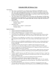
Figure 3.1 contains the system architecture.
USER
r/w
connect, accept,
register, query
query result
I/O
query result
DISPATCH
r/w
I/O
accepted, connected,
registered, query
r/w
I/O
listen
r/w
Figure 3.1: The system architecture.
3.2
Basic Asynchronous Sockets
An asynchronous model for sockets, aside from the performance benefits associated with being built on top of select,
offer the chance to greatly reduce programmer error through a concise API and well-defined set of usage conventions.
First, they focus the programmer’s attention on implementing just a few callback points, and free him/her from having
to explicitly manage the life cycle of a socket, let alone remember it. Callbacks fire as things happen to the underlying
socket. If there’s data to read, the onReceive handler will fire and compel the callee to respond accordingly; this scenario is in contrast to the synchronous model, whereby responsibility for operating the underlying socket, in addition
to the above, falls upon the user. Second, we point out that callbacks are serial and, by implication, thread-safe. Thus,
instead of having to synchronize the actions of each thread in the one-thread-per-socket model, one can simultaneously preside over many sockets while at the same time programming as if there were only client in the system. In the
subsections that follow, we describe the API exposed by the org.shared.net package. An overview schematic can be
found there.
3.2.1 Connection
The Connection interface defines callbacks that all asynchronous sockets must implement. Table 3.1 and Figure 3.2
describe the function of each callback, along with its place in the broader connection lifecycle. A connection starts out
unbound, in the sense that it does not yet have a socket associated with it. Upon calling init(InitializationType, ConnectionHandler, Object) with InitializationType#CONNECT or InitializationType#ACCEPT, the user declares an
3.2: BASIC ASYNCHRONOUS SOCKETS
33
interest in accepting on some local address or connecting to some remote address, respectively. Notice that ServerSockets have no role in this process, and are completely hidden from the user. Alternatively, should one desire to
offer an existing SocketChannel for management, one may bypass the above procedures and directly register it using
init(InitializationType, ConnectionHandler, Object) with InitializationType#REGISTER. Upon successful binding of the connection to a physical socket, the system will invoke the onBind() callback, or onClosing(ClosingType,
ByteBuffer) with ClosingType#ERROR if the request could not be fulfilled. Afterwards, the system will invoke
the onReceive(ByteBuffer), onClosing(ClosingType, ByteBuffer), and onClose() callbacks to denote that new
data has arrived, that the connection is being closed, and that a close operation has completed, respectively. In the
meantime, the user may invoke the thread-safe send(ByteBuffer) method to send data to the remote host. In the spirit
of asynchronous sockets, every implementor must make the guarantee that send never blocks. Whereas traditional
sockets preserve data integrity by blocking the writing thread, it remains the implementor’s responsibility to enqueue
data that could not be written out to the network in a temporary buffer. At any given time during the above process,
the system may invoke onClosing with ClosingType#ERROR to signal an error with the underlying socket, and the
user may invoke close() to shut down the connection.
method
onBind()
onReceive(ByteBuffer)
onClosing(ClosingType, ByteBuffer)
onClose()
init(InitializationType, ConnectionHandler, Object)
send(ByteBuffer)
setException(Throwable)
getException()
close()
description
on bind of the underlying socket, whether by connecting
or accepting on a ServerSocket
on receipt of data
on connection closure
on completion of connection closure
connects to the remote address, accepts on the local address, or registers an existing SocketChannel for management; returns immediately with a completion Future
sends data; returns immediately and enqueues remaining
bytes if necessary
delivers an error to this connection
gets the error that occurred
closes the connection
Table 3.1: Methods defined by the Connection interface.
3.2.2
NioConnection and ConnectionManager
As its name implies, the NioConnection class is the SST’s (partial) implementation of the Connection interface
that relies on an external entity, ConnectionManager, to invoke callbacks and hide the prodigious amounts of bookkeeping involved in the connection lifecycle (see Figure 3.2). Before interacting with a subclass instance of NioConnection, one must first register it with an instance of ConnectionManager via the required argument in the
NioConnection constructor. After registration, the connection is thereafter managed, in that all callbacks happen in
the ConnectionManager thread. Aside from typical errors like connection reset that can happen from underlying
sockets, the manager will also deliver an error on shutdown, or in the event that some callback throws an unexpected
exception.
In a nutshell, managed connections provide mechanisms that underlie the Connection interface and its associated
lifecycle. The org.shared.net package hides all inner workings from the user, allowing him or her to concentrate on
implementing the callbacks that matter to the specific task, namely onBind, onReceive, onClosing, and onClose.
Thus, protocol designers can have the proverbial scalable networking cake and eat it too, with the help of a greatly
simplified programming interface.
34
CHAPTER 3: ASYNCHRONOUS NETWORKING
VIRGIN
accept /
listen
connect /
connect
ACCEPT
CONNECT
on accept
on connect
on end-of-stream,
on close
ACTIVE
write buffer
emptied
writes
deferred
user request
enable
write
through
read
enabled
read
disabled
CLOSING
write buffer
remaining
user request
disable
on error
CLOSED
bytes written
Figure 3.2: The Connection lifecycle.
3.3
High Level Semantics
Understanding a networking stack is like peeling away the layers of an onion – Each upper layer wraps a lower
layer and adds specialization. Just as TCP/IP is built on top of IP, which itself is built on top of the link layer, the
org.shared.net package has its own hierarchy in which we extend the functionality of managed connections laid out
by Subsection 3.2.2. The hierarchy of abstractions found in Table 3.2 are listed in decreasing order of specificity.
We point out that, on top of basic asynchronous behavior, the SST networking package has two additional goals –
First, to emulate synchronous behavior, should the user desire that style of programming; and second, to support a
messaging layer for custom protocol design. In the ensuing subsections, we discuss these extensions and how they
may potentially simplify the task of writing networked programs.
3.3.1 SynchronousHandler
The SynchronousHandler is an implementation of ConnectionHandler that supports a pair of input/output streams
for communications. One might question the point of emulating synchronous behavior in the first place; after all,
the venerable java.net.Socket class already works quite well. Reimplementing blocking semantics on top of the
3.3: HIGH LEVEL SEMANTICS
35
class
XmlHandler
SynchronousHandler
NioConnection
java.nio
TCP/IP
description
(de)serialization of semantic events
additional synchronous behavior
basic asynchronous behavior
non-blocking sockets
transfer layer provided by the OS
Table 3.2: The org.shared.net abstraction stack.
SST’s networking package has multiple benefits, however – First, one can consolidate synchronous and asynchronous
connections under a common infrastructure; second, the purely additive API exported synchronous connections does
not disable any asynchronous functionality; and third, the networking layer, still presided over by a single thread,
retains its scalability.
In Table 3.3, we describe the additional methods that synchronous connections offer. Broadly speaking, the above
methods are friendliest to program logic that pulls data and results from objects, rather than reacting to notifications
pushed to it via callbacks. To illustrate usage, see the code snippet below that depicts a server listen-and-accept
loop. Notice how the actions of creating a ServerSocket, binding it to an address, and accepting a connection are
completely hidden from the user.
method
getInputStream()
getOutputStream()
getLocalAddress()
getRemoteAddress()
description
gets an input stream from this handler
gets an output stream from this handler
gets the local socket address
gets the remote socket address
Table 3.3: Additional methods provided by the SynchronousHandler class.
public class Test {
public static void main(String[] args) throws Exception {
int port = 1234;
int backlogSize = 64;
int bufSize = 4096;
InetSocketAddress bindAddr = new InetSocketAddress(port);
ConnectionManager<NioConnection> cm = NioManager.getInstance().
setBacklogSize(backlogSize);
for (;;) {
SynchronousHandler<Connection> handler = new SynchronousHandler<
Connection>("Client Handler", bufSize);
Future<?> fut = cm.init(InitializationType.ACCEPT, handler,
36
CHAPTER 3: ASYNCHRONOUS NETWORKING
bindAddr);
// Block until success or error.
fut.get();
}
}
}
3.3.2 XmlHandler
As is common for distributed systems, the programmer has a high level control protocol for coordinating disparate
machines over a network. Ideally, he or she would, in addition to having to specify the protocol, spend a minimal amount of time actually implementing it. Metaphorically speaking, sending and receiving events correspond to
Connection#send(ByteBuffer) and ConnectionHandler#onReceive(ByteBuffer), respectively. To formalize this,
we introduce XmlHandler, an implementation of ConnectionHandler specially designed to transport XmlEvents.
Before discussing the features of XmlHandler, we briefly describe the org.shared.event package, which provides
foundation classes for defining, processing, and manipulating events:
• The Event interface is parameterized by itself, and defines every event as having a source retrievable via
Event#getSource(). Subsequently, XmlEvent implements Event and assumes/provides (de)serialization routines for the DOM representation.
• The Source interface defines an originator of Events. It extends SourceLocal and SourceRemote, which
themselves define local and remote manifestations – that is, one should consider an invocation of SourceRemote#onRemote(Event) as sending to the remote host and SourceLocal#onLocal(Event) as receiving from
the remote host.
• The Handler interface defines anything that can handle events and react accordingly. One can effectively modify
the behavior of Source objects with the Source#setHandler(Handler) and Source#getHandler() methods.
• The EventProcessor class is a thread that drains its event queue in a tight loop. The queue is exposed to the
rest of the world by virtue of EventProcessor implementing SourceLocal.
The reader has probably inferred by now that XmlHandler encourages an event-driven programming model. Table
3.4 lists the available methods, while Figure 3.3 attempts to place them in context. Note that parse(Element) and
onRemote(XmlEvent) correspond to send and onReceive, respectively; we also leave parse abstract, with the
expectation that only the user knows how to reconstruct events from DOM trees. Assuming that the alive entities
consist of a EventProcessor instance, a ConnectionManager instance, and the remote machine (treated as a black
box), Figure 3.3 depicts the delegation chains by which they would intercommunicate.
method
parse(Element)
createEos()
createError()
onRemote(XmlEvent)
getHandler()
setHandler(Handler)
description
parses an event from a DOM Element and fires it off;
null input denotes an end-of-stream
creates an end-of-stream event
creates an error event
sends an event to the remote host
gets this connection’s event handler
sets this connection’s event handler
Table 3.4: Additional methods provided by the XmlHandler class.
3.3: HIGH LEVEL SEMANTICS
37
outbound
inbound
SSL/TLS
decrypt
parse
DOM
parse
event
server logic
client logic
SSL/TLS
encrypt
inbound
DOM
to bytes
event to
DOM
outbound
Figure 3.3: The event-driven model supported by the XmlHandler class.
To begin with, suppose the connection manager receives an XmlEvent, given as bytes, from the remote machine.
It invokes the onReceive method of XmlHandler, which is overridden to call parse. An XmlEvent results and
is passed off to the event processor via onLocal. Next, the event processor, upon reacting to the event, decides to
create a new event and contact the remote machine – It calls onRemote, which is overridden to serialize its input and
call send. Finally, the remote machine receives an event, processes it, and the cycle repeats. Note that Figure 3.3
represents a microcosm of the communication layer in practice – The local machine could potentially have thousands
of connections with remote machines.
The SST asynchronous networking API by no means restricts the user to the classes described above. In fact, one
can override any level of the protocol stack, with the choice dependent on the level of specific functionality desired.
By compromising among power, flexibility, and conciseness, the org.shared.net package attempts to consolidate all
TCP-based connections on top of a single foundation, and makes no distinction among the semantics that differ from
one connection to another.
38
CHAPTER 3: ASYNCHRONOUS NETWORKING
Chapter 4
Utilities
The SST tries to make scientific programming easier by providing a Swiss army knife of tools for the scientific
programmer. Although many of the methods found herein are individually and immediately useful, together they
constitute a way of doing things. Thus, with sufficient familiarity of the underlying APIs, one can have preliminary,
out of the box answers for issues ranging from process management to logging to concurrency control.
4.1
A Convenience Class
The org.shared.util.Control and org.shared.util.IoBase classes try to free the programmer from having to write
tedious, boilerplate code that wastes screen space and effort. You might find many of its simplifications useful:
• Many I/O devices have a close method and implement Closeable on the side. If you don’t care about a possible
IOException, consider typing
IoBase.close(stream);
instead of
try {
stream.close();
} catch (IOException e) {
}
In a similar vein, the Thread#sleep method is a hint at best. If you don’t care about getting woken up prematurely, consider typing
Control.sleep(millis);
instead of
try {
Thread.sleep(millis);
} catch (IOException e) {
}
• Spawning processes is easy. To run the rm program with arguments -f and foo, type
IoBase.execAndWaitFor("rm", "-f", "--", "foo");
39
40
CHAPTER 4: UTILITIES
The JVM will fork-exec, and the calling thread will block until completion. Communications with the child is
also supported with input and output streams. To pipe the cat program’s output into System.out while feeding
it an array of bytes, type
IoBase.execAndWaitFor(new ByteArrayInputStream(inArray), System.out,
System.err, workingDir, "cat");
The implementation of process control is deadlock safe – calls to IoBase#execAndWaitFor spawn reader and
writer threads to handle the child’s input, output, and error output streams.
• Control contains quite a few assertion “macros” for checking values and maintaining invariants. Failure of
checks results in a RuntimeException or AssertionError. To extract the equality value of two ints and throw
an exception otherwise, consider typing
int eq = Control.checkEquals(a, b, "Invalid arguments");
instead of
int eq;
if ((eq = a) != b) {
throw new RuntimeException("Invalid arguments");
}
• Measuring execution wall clock time is easy with Control#tick and Control#tock, two operations reminiscent
of MATLAB’s tic and toc. To take a measurement, type
Control.tick();
doActions();
System.out.printf("Time elapsed: %d ms%n", Control.tock());
Note that pairs of these operations are scoped to the current thread via a ThreadLocal static member storing the
elapsed time.
• Deleting files or directories is possible with IoBase#delete. One should use this method with care, as it
recursively deletes any directories encountered without following symbolic links.
• Stream-to-stream, stream-to-file, and file-to-stream transfers are possible through IoBase#transfer and its variants. To use, one types
InputStream in = FileInputStream("data.in");
OutputStream out = FileOutputStream("data.out");
IoBase.transfer(in, out);
out.close();
4.2
Logging
The org.shared.log package contains useful methods for creating and manipulating logs. By convention, the SST
ships with Log4J as its logging backend and SLF4J as its logging frontend. In other words, Log4J implements logging
4.2: LOGGING
41
to files, streams, and sockets, while SLF4J (Simple Logging Facade for Java) provides an abstraction layer that allows
interchangeability of the former with any number of other logging frameworks.
The preferred way of using SST logging is to create an SLF4J Logger instance from a LoggerFactory and then
configure Log4J underneath. For convenience, the user may load a Log4J XML configuration file found on the class
path with the static method Logging#configureLog4J. The code snippet below demonstrates how to set up a logging
environment for running unit tests:
public class LoggerDemo {
final protected static Logger log = LoggerFactory.getLogger(Tests.class);
static {
Logging.configureLog4J("org/shared/log4j.xml");
Logging.configureLog4J("org/shared/net/log4j.xml");
Logging.configureLog4J("org/shared/test/log4j.xml");
}
}
42
CHAPTER 4: UTILITIES
Chapter 5
Annotation-driven APIs
Of the language features introduced in Java 1.5, annotations have seen particularly heavy use, and for good reason.
Conceptually, code annotations are another level of indirection, in that they separate specification from implementation
– oftentimes, one should be able to say how a program is supposed to work without writing the control flow logic to
make it happen. Many tasks that would either be tedious, ad hoc, and/or ill-defined can be addressed with a declarative
programming model that necessitates only the specification part. In the ensuing sections, we demonstrate how the SST
provides complex functionality hidden behind the facade of multiple annotation-driven APIs, which handle everything
from resource loading to encoding finite state machines to parsing of command-line arguments.
5.1
Resource Loading Rules as Annotations
If you’ve ever written a Java program that depends on Jar’d third party packages, then you’ve probably had to specify
an overly long classpath when starting up the JVM. As the number of dependee packages grows, appending to the
classpath becomes an unwieldy solution that exposes the needs of your program to the outside world.
The Toolbox resource loader found in org.shared.metaclass.Loader is a workable solution to Jar madness by
inserting a level of indirection between the startup of the JVM and the actual loading of your program – you invoke
Loader’s main method and tell it the entry point of your program. Consequently, the loader expects that your program
has class-level annotations that specify the packages needed for successful execution. It will prepare these for you on
the classpath of a custom classloader, which it then uses to call into your code.
5.1.1
Program-level Annotations
To invoke Loader on a target class packageName.className, type
java org.shared.metaclass.Loader packageName.className
Any further arguments will be forwarded as arguments to packageName.className. One decorates programs with
annotations to direct loading behavior:
• @EntryPoint – Marks the entry point called into by Loader.
• @LoadableResources – A container for an array of resource descriptions.
The Toolbox distribution itself contains programs that bootstrap from the resource loader. The test driver test.All,
shown below, has three resource requirements – the Jar’d JUnit testing package (at bin/lib/junit.jar), Apache Commons
Logging (at bin/lib/commons-logging.jar), and the SST native library (at bin/lib/libshared.so, assuming UNIX naming conventions divined from System#mapLibraryName). Notice that the declaration syntax is in the style of fully
43
44
CHAPTER 5: ANNOTATION-DRIVEN APIS
qualified Java class names, and that the type of resource followed by a colon precedes the resource name for name mapping purposes. Thus, jar:foo.bar.jarfile refers to the class path location foo/bar/jarfile.jar, and native:foo.bar.library
refers to foo/bar/liblibrary.so. The method marked with @EntryPoint is a vanilla main method. A code snippet is
provided below. We describe the use of the @LoadableResources#packages field in Subsection 5.1.2.
@LoadableResources(resources = {
//
"jar:lib.commons-codec", //
"jar:lib.junit", //
"jar:lib.log4j", //
"jar:lib.slf4j-api", //
"jar:lib.slf4j-log4j12" //
}, //
//
packages = {
//
"org.shared.test" //
})
public class All {
...
/**
* The program entry point.
*/
@EntryPoint
public static void main0(String[] args) {
...
}
...
}
5.1.2
Package-level Annotations
In combination with the org.shared.metaclass package, the SST resource loader provides users with fine-grained
control over how classes are loaded. As mentioned in Subsection 5.1.1, the @LoadableResources#packages
field denotes those packages whose classes depend, for linking purposes, on loaded Jars and libraries. To mark
them as such, one employs the @Policy package-level annotation, which directs the behavior of an underlying RegistryClassLoader. One first creates a package-info.java file in the target package’s directory, and then attaches a
@Policy instance to the package keyword. The code snippet below demonstrates how this would work on the shared
package.
// File "src_test/org/shared/test/package-info.java".
@Policy(recursive = true, //
//
includes = {
5.2: FINITE STATE MACHINES AS ANNOTATIONS
45
//
"org.shared.codec", //
"org.shared.log", //
"org.shared.net" //
})
package org.shared.test;
import org.shared.metaclass.Policy;
Policies may declare the @Policy#recursive element (default true) – that is, the user may specify whether the
underlying RegistryClassLoader will initiate loading of the target package and its subpackages. Annotating a subpackage will override its parent package’s policy for all subsequent subpackages; for it to take effect, one still needs to
explicitly declare it in the @LoadableResources#packages field. Policies may also declare a @Policy#includes
field (default empty), which, like a macro, contains external packages and classes. The underlying RegistryClassLoader will recursively inspect the @Policy annotations of included packages, while recording included classes as
requiring special treatment. Note that one distinguishes an included class by the ‘#’ character that separates the package name from the class name.
The SST resource loader, with its declarative programming interface, offers the user a great amount of leverage
and flexibility with regards to linking the resources necessary for program execution. In essence, the APIs described
above allow one to eschew the traditional, fixed notion of a class path and carve it up into those domains that require
linking to loaded resources (via RegistryClassLoader) and those that don’t (via the parent class loader). With this
power, however, a user unfamiliar with the guts of Java class loading can quickly run into exotic LinkageErrors that
utterly confound at first glance. Consequently, proper annotation discipline stems from the realization that problems
arise from two cases – first, when the parent class loader attempts to link a resource exclusive to the underlying
RegistryClassLoader; and second, when both class loaders end up loading multiple copies of a class. To avoid the
above problems and as a general rule of thumb, packages and classes visible only to the resource loader should link to
those that are also visible to the parent class loader, and not the other way around.
Generally speaking, the intricacies of Java’s class loading and linking rules are beyond the scope of this document;
for a more complete overview, please see Chapter 5 of the virtual machine specification. Although the errors that
emerge from improper use of the Loader construct may at times be mind-bendingly bizarre, we feel that the logistical
and conceptual savings of having a flexible, expressive, and mostly transparent class loading discipline outweigh the
downsides.
5.2
Finite State Machines as Annotations
The org.shared.event package, with its message passing model, relies heavily on the concept of finite state machines,
which in turn are declared via annotations. Recall that a finite state machine is a set of states and transitions among
states. In org.shared.event, states are represented by Enums and transitions are declared with the @Transition
field-level annotation (@Transitions for multiple). A @Transition instance has four fields: currentState for the
current state, nextState for the next state, eventType for the Event Enum type of interest, and group for the logical
grouping. To use it, one attaches a @Transition (or @Transitions, which contains an array of the former) to a
Handler field. Such an association would declare said Handler as firing when said Event type, current state, and
group name co-occur. Upon handling the event, the underlying EnumStatus (a mutable state entity) transitions to the
next state, if specified.
With the finite state machine API in mind, users need to provide three things: the handlers for every foreseeable (state × event type) pair, their associated transitions, and the StateTable(Object, Class<X>, Class<Y>)
constructor, where X is the state Enum type and Y is the event Enum type. The code snippet below, taken from
src_net/org/shared/net/nio/NioManagerThread.java, demonstrates how state machines drive the asynchronous
networking layer described in Chapter 3:
46
CHAPTER 5: ANNOTATION-DRIVEN APIS
public class NioManagerIoThread extends NioManagerThread {
@Override
protected void onStart() {
initFsms();
}
...
@Transition(currentState = "ACTIVE", eventType = "OP")
final Handler<NioEvent<Integer>> opHandler = new Handler<NioEvent<Integer
>>() {
@Override
public void handle(NioEvent<Integer> evt) {
int opMask = evt.getArgument();
handleOp((NioConnection) evt.getSource(), opMask & 0x7FFFFFFF, (
opMask & 0x80000000) != 0);
}
};
@Transition(currentState = "ACTIVE", eventType = "CLOSE")
final Handler<NioEvent<?>> closeHandler = new Handler<NioEvent<?>>() {
@Override
public void handle(NioEvent<?> evt) {
handleClosingUser((NioConnection) evt.getSource());
}
};
@Transitions(transitions = {
//
@Transition(currentState = "ACTIVE", eventType = "ERROR"), //
@Transition(currentState = "CLOSING", eventType = "ERROR") //
})
final Handler<NioEvent<Throwable>> errorHandler = new Handler<NioEvent<
Throwable>>() {
@Override
public void handle(NioEvent<Throwable> evt) {
handleError((NioConnection) evt.getSource(), evt.getArgument());
}
};
...
}
abstract public class NioManagerThread extends Thread //
5.2: FINITE STATE MACHINES AS ANNOTATIONS
47
... {
...
/**
* Initializes the underlying {@link StateTable}s.
*/
protected void initFsms() {
this.fsm = new StateTable<NioConnectionStatus, NioEventType, NioEvent
<?>>( //
this, NioConnectionStatus.class, NioEventType.class);
this.fsmInternal = new StateTable<NioManagerThreadStatus, NioEventType
, NioEvent<?>>( //
this, NioManagerThreadStatus.class, NioEventType.class, "
internal");
}
...
/**
* The external state machine.
*/
protected StateTable<NioConnectionStatus, NioEventType, NioEvent<?>> fsm;
/**
* The internal state machine.
*/
protected StateTable<NioManagerThreadStatus, NioEventType, NioEvent<?>>
fsmInternal;
...
}
When using the API, keep in mind that:
• The wildcard "*" is permitted for states and event types.
• The target object’s class and all superclasses will be searched for declared Handler fields.
• The @Transition group name allows you to associate various transitions on the same handler with different finite
state machines, which one declares with the alternate constructor StateTable(Object, Class<X>, Class<Y>,
String).
• The nextState field is optionally; feel free to handle your own state transitions.
• Use the EventProcessor thread class to drive finite state machines. A common architecture would involve
multiple processors communicating to each other via message queues, which dispatch as (state × event type)
lookups.
48
CHAPTER 5: ANNOTATION-DRIVEN APIS
5.3
Command-Line Arguments as Annotations
Specifying and parsing command-line arguments for a program is best left to libraries like Apache Commons CLI.
While powerful and useful, Commons CLI still requires considerable amounts of control flow logic for laying out the
kinds of arguments encountered. Consequently, the SST’s own CLI implementation, manifested in the org.shared.cli
package, uses Commons CLI underneath while exporting command-line argument specifications as the @CliOptions
and @CliOption class-level annotations. With them, one merely annotates a class and analyzes it with Cli#createCommandLine.
Additionally, a help string may be created with Cli#createHelp. The code snippet below demonstrates how a simple
program might be annotated and how it would print out a help message:
@CliOptions(options = {
//
@CliOption(longOpt = "host", nArgs = 1, required = true, description =
"the hostname"), //
@CliOption(longOpt = "port", nArgs = 1, required = true, description =
"the port number"), //
@CliOption(longOpt = "use-ssl", nArgs = 0, description = "whether or
not to use SSL") //
})
public class ConnectorProgram {
public static void main(String[] args) throws Exception {
// Display the help string.
System.out.println(Cli.createHelp(ConnectorProgram.class));
// Create the command-line data structure.
CommandLine cmdLine = Cli.createCommandLine(ConnectorProgram.class,
args);
// Main program logic goes here.
}
}
>>
--host
--port
--use-ssl
the hostname
the port number
whether or not to use SSL
Chapter 6
Parallel Dataflow Engines
The org.shared.parallel package provides interfaces and classes for defining atomic units of work, their dependencies, and the means to automatically execute them in parallel on multicore machines. A parallel dataflow engine, or
just engine, is a construct for performing a set of calculations in parallel to the fullest extent that their dependencies
allow. By decoupling the execution of a parallel computation from the actual coding of it, engines have the potential
to save scientific programmers significant amounts of time. In fact, by taking an opportunistic approach to execution,
where an atomic calculation is performed as soon as its dependencies are met, engines can actually make a computation
faster than all but the most optimized hand coding.
In the SST’s implementation, engines are backed by a java.util.concurrent thread pool hidden from the user.
Consequently, it remains the user’s responsibility to implement the atomic calculations that make up the computation
as well as specify what calculations feed other calculations. One can think of engine execution along the lines of
pushing data from a source node to a sink node – any in edges to nodes represent inputs to their respective calculations.
Likewise, any out edges represent outputs. See Figure 6.1 for an illustration.
2x (1)
Start () (0)
x (4)
+ (3)
I (2)
+ (6)
2x (7)
O (8)
Stop () (9)
- (5)
Figure 6.1: An illustration of a toy engine that takes an integer input and has an integer output. The start node (green
diamond) immediately feeds its dependent calculation nodes (blue rectangles). To review calculation node notation,
“2×” is doubling, “I” is identity, “+” is summation, “×” is product, and “−” is subtraction. The output, denoted
“O”, contains an observable output – hence its shape as a red octagon. The stop node (green diamond) is just a
logical marker signaling the end of the computation. The numbers in parentheses represent a traversal ordering that
does not violate dependency constraints if a single thread were to walk the dataflow graph. In this example, sending
in a value of 1 yields a value of 8 at the output node.
6.1
Usage
The org.shared.parallel package is supported by four concept classes:
• Calculator – Defines atomic units of work.
• Handle – Stores values; effectively remembers outputs so they can be observed.
49
50
CHAPTER 6: PARALLEL DATAFLOW ENGINES
• TraversalPolicy – Guides traversal of the dataflow graph by multiple threads.
• Engine – Executes a parallel computation.
Once a user has implemented them, she has effectively defined a parallel computation. To demonstrate with a toy
example, we pull out a JUnit test corresponding to the engine shown in Figure 6.1. First, we define a series of
calculator nodes.
...
static class Summer implements Calculator<Integer, Integer> {
@Override
public Integer calculate(List<? extends Handle<? extends Integer>>
inputVector) {
int sum = 0;
for (int i = 0; i < inputVector.size(); i++) {
sum += inputVector.get(i).get().intValue();
}
return sum;
}
@Override
public String toString() {
return "+";
}
}
...
Second, we instantiate an Engine parameterized to Integer, its input type. Third, we instantiate a series of calculations
that take integers as input and spit out integers as output. Notice that we define an output node from which we can
derive a Handle that is a reference to the computation result. Fourth, we register atomic calculations with the engine,
where the add method takes a dependent calculation followed by its dependees. The registration of the output node is
different in that we derive a Handle from it. Fifth and finally, we execute the engine on an argument of 1 and expect
an output of 8.
...
public void testExecute1() {
Calculator<Integer,
Calculator<Integer,
Calculator<Integer,
Calculator<Integer,
Calculator<Integer,
Calculator<Integer,
Integer>
Integer>
Integer>
Integer>
Integer>
Integer>
r1
d1
s2
s1
m1
a2
=
=
=
=
=
=
new
new
new
new
new
new
Repeater();
Doubler();
Summer();
Subtractor();
Multiplier();
Summer();
6.1: USAGE
51
Calculator<Integer, Integer> d2 = new Doubler();
Calculator<Integer, Integer> o1 = new Outputter();
this.engine.add(r1, this.engine.getInput());
this.engine.add(d1, this.engine.getInput());
this.engine.add(s2,
this.engine.add(s1,
this.engine.add(m1,
this.engine.add(a2,
this.engine.add(d2,
r1, d1);
r1, s2);
d1, s2);
s1, m1);
a2);
Handle<Integer> ref = this.engine.addOutput(o1, d2);
this.engine.execute(1);
assertEquals(new Integer(8), ref.get());
}
...
The rules of parallel execution are simple: if a node’s inputs have all been computed, then that node may commence
execution; if a node’s outputs have all been observed by dependents, then that node’s stored value may be cleared and
potentially garbage collected. Such actions are reflected in the loops of Procedure 1. Consequently, engines prepare
a calculation node for parallel execution by setting the in count equal to the number of dependees and the out count
equal to the number of dependents. Traversal orderings play their part by determining the priority of various enqueued
calculations; notice that the correctness of the computation does not depend on the priority.
Let q be a (priority) work queue of the thread pool;
Let this denote the current node;
for c ∈ this.out do
c.incount ← c.incount − 1;
if c.incount = 0 then
Enqueue(q, c);
end
end
Calculate(this, this.in);
for c ∈ this.in do
c.outcount ← c.outcount − 1;
if c.outcount = 0 then
Clear(c);
end
end
Algorithm 1: An atomic calculation’s interaction with the work queue.
There are two major restrictions to the usage of Engine. First, a semaphore guards the Engine#execute method,
which means that calls to it can’t be pipelined. If it’s any consolation, remember that the engine execution itself is
parallelized. Second, a calculation node may only be added if it doesn’t already exist and if its dependees have been
added. This policy makes the implementation simpler by enforcing an implicit topological ordering.
52
CHAPTER 6: PARALLEL DATAFLOW ENGINES
6.2
Finding the Right Topological Sort
To formulate an engine execution plan consistent with data dependencies, we use topological sort to derive a total
ordering over the calculation nodes. We define the TraversalPolicy interface as an abstraction for providing traversal
orderings over dataflow graphs. At first glance, deferring the implementation of topological sort seems somewhat
esoteric, since program correctness should not depend on any specific ordering. As we will show below, however,
the implementation of TraversalPolicy very much determines other properties of parallel computation, like memory
footprint.
a
I (1)
+ (3)
I (2)
I (4)
Start () (0)
+ (5)
I (6)
+ (7)
+ (9)
O (10)
Stop () (11)
+ (9)
O (10)
Stop () (11)
I (8)
b
I (5)
+ (6)
I (4)
Start () (0)
I (3)
+ (7)
I (2)
+ (8)
I (1)
Figure 6.2: Comparison of memory optimal and memory suboptimal orderings. The differences are circled by
the dotted red line. a) the ordering imposed by LimitedMemoryPolicy; b) the ordering imposed by a particularly
wasteful, hypothetical policy.
We explore one particular policy, which is LimitedMemoryPolicy. As its name suggests, this policy attempts
to minimize (over all orderings) the maximum memory footprint (over all stages of the computation). Consider, for
simplicity’s sake, an engine backed by a single thread and its execution under orderings optimized and not optimized
for memory usage, respectively, in Figure 6.2. The example contains identity nodes labeled “I” and summation nodes
labeled “+”. Suppose that it takes 1 unit of memory to store the output of an identity node. Consequently, it’s not
hard to see why the maximum memory usage at any point in time for the topology in Figure 6.2-a is 2 units – as the
6.2: FINDING THE RIGHT TOPOLOGICAL SORT
53
execution engine walks the graph, it’s required to hold on to no more than 2 outputs at any given time. On the other
hand, the maximum memory usage at any point in time for the topology in 6.2-b is 5 units – the execution engine must
hold on to the outputs of all identity nodes before it can even begin pushing them through the summation nodes. In
fact, one can make an arbitrarily wasteful ordering by extending the above examples to analogies of size n which have
an O(n) memory footprint (as opposed to the optimal footprint of 2).
We present the algorithm behind LimitedMemoryPolicy in Algorithm 2, which is essentially a modified version
of the standard depth first search (DFS) used to determine a topological ordering. At a high level, our algorithm does
the obvious: execute calculations furthest away from the stop node (by graph theoretic distance) first to minimize the
maximum number of simultaneously held, intermediate outputs. The result is a procedure named LongestPath that
sorts each node’s children by the maximum distance to the sink. Thus, by running LongestPath as a precursor to
DFS, the algorithm attempts to execute deep calculations first with the aim of aggressively reclaiming their outputs.
Let this denote the current node;
Let children denote the dependees;
maxDistance ← −1;
for child ∈ children do
if Not(IsVisited(child)) then
/* Recurse on the child.
LongestPath (child);
end
maxDistance ← Max(maxDistance, Distance(child));
end
Sort (children);
SetVisited (this, true);
SetDistance(this, maxDistance + 1);
Algorithm 2: The procedure LongestPath.
*/
54
CHAPTER 6: PARALLEL DATAFLOW ENGINES
Chapter 7
Image Processing
There are statistical patterns in the world all around us, both in time and space. To make sense of it all on a computer,
one often employs digital signal processing (DSP) techniques. The DSP field itself is too broad to cover in one chapter; instead, we survey the small subset implemented by the SST packages org.shared.fft and org.shared.image.
These packages specialize in the fast Fourier transform (FFT) and 2-D image processing. They are meant to appeal to
beginners and veterans alike – beginners will find ready-to-use filters built on top of the already familiar multidimensional array package org.shared.array; likewise, veterans may benefit from the advanced capabilities like convolution
kernel caching and a complete, tunable interface to FFTW3.
7.1
Supported Operations
From a library design point of view, ever more complex numerical calculations demand functionality not found in the
generality of base classes. Just as the SST array package frees the user from the tedium of managing multidimensional
data as flat arrays, the image processing and FFT packages strive to eliminate the need for writing idiomatic sequences
of signal analysis operations over multidimensional arrays themselves. With the introduction of extensive caching and
acceleration mechanisms, we look to enable the user to write concise code that is at the same time competitive with
the hand-optimized performance.
7.1.1
ConvolutionCache
The ConvolutionCache class serves both as a convenient way to convolve signals (in our case images) with filters,
and as a way to cache parts of previous computations to speed up current ones. Before detailing the optimizations
found therein, we digress to a discussion of convolution both in general terms and in context of the image processing
use case.
As the user may recall from the famous convolution theorem, the Fourier transform of a convolution of two (for
our purposes discrete time) signals is the pointwise product of their Fourier transforms. Symbolically, if F denotes
the Fourier transform, and s and t represent signals, this amounts to
F(s ∗ t) = F(s) · F(t)
s ∗ t = F −1 (F(s) · F(t)).
Written programmatically, if s and t are multidimensional arrays, their convolution is given by
s.fft().eMul(t.fft()).ifft();
or, alternatively,
55
56
CHAPTER 7: IMAGE PROCESSING
s.rfft().eMul(t.rfft()).rifft();
In image processing, one very frequently applies a collection of variable size filters to each of a collection of fixed size
images. Recall that each convolution requires padding a filter to the size of its target image, and then performing the
sequence of operations mentioned above. For an image im and a filter f, their convolution is given by
im.fft().eMul(pad(f, im.dims()).fft()).ifft();
How might one speed up convolutions for image processing in the common case? A cursory examination reveals
that, if indeed most images have the same size, then the padded and transformed filter can be cached. Furthermore, one
can precompute the FFT of the image. Thus, with the help of ConvolutionCache, only two operations are required –
namely, a pointwise multiplication and an inverse FFT, and the calculation comes out to
imTransformed.eMul(fPaddedTransformed).ifft();
We bundle the above operations in the ConvolutionCache#convolve method, which takes a transformed image and
an unpadded, untransformed filter as arguments. Note that the cache hides all details of maintaining possibly many
copies of the same filter for different image sizes. The user need not worry about memory management either, as the
cache uses the SoftReference class – the JVM automatically reclaims underlying cache entries when it starts to run
out of memory.
7.1.2
Filters
The org.shared.image.filter package contains a variety of predefined convolution kernels, or filters, for 2-D image
processing. Currently, it supports complex-valued Gabor, circular Gabor, and {0th, 1st} derivative of Gaussian filters,
as shown in the heatmaps of Figure 7.1. We design said filters to interoperate with ConvolutionCache, which means
that they fulfill the Object#equals and Object#hashCode contracts.
a-1
a-2
b-1
b-2
c
0
Figure 7.1: A visual index of the filters offered by the image processing package. a) a complex-valued Gabor filter
oriented at π/4 with frequency 2 shown as real and imaginary parts, respectively; b) a complex-valued circular Gabor
filter with frequency 2 shown as real and imaginary parts, respectively; c) a steerable, 1st derivative of Gaussian filter.
7.1.3
IntegralImage and IntegralHistogram
The IntegralImage and IntegralHistogram classes provide a memoization scheme for computing sums and histograms, respectively, over rectangular regions of multidimensional arrays in time linear in the number of dimensions
(not dependent on the region size). They have seen extensive use in computer vision [6]. Although the number of
dimensions for the IntegralImage#query(int...) method usually is two for intensity images, the IntegralImage constructor accepts arrays with an arbitrary number of dimensions d. Note that the query arguments a1 , b1 , . . . , ad , bd
ask for the sum over the hypercube induced by the Cartesian product [a1 , . . . , b1 ] × . . . × [ad , . . . , bd ]. Similarly, the
7.2: SAMPLES
57
IntegralImage#query(double[], int...) method yields the histogram over said hypercube. To initially bin the values
of some input array, the IntegralHistogram constructor accepts, along with the number of classes, an IntegerArray
argument that describes class memberships.
7.1.4
FFTW3 Interface
The sharedx.fftw extensions package strives to provide a full-featured JNI interface to the popular FFTW3 [2] library.
To integrate with SST multidimensional arrays, it exports FFTW operations through FftwService, an implementation of the FftService interface. Through the generic hinting methods FftService#getHint(String) and FftService#setHint(String, String), users are able to get and set FFTW-specific attributes and data:
• Setting values “estimate”, “measure”, “patient”, and “exhaustive” for the hint “mode” will adjust the amount of
desired precomputation from FFTW.
• Setting a value for the hint “wisdom” imports FFTW wisdom in string form into the native layers. Conversely,
getting the “wisdom” hint will ask FFTW to export its learned wisdom to string form.
7.2
Samples
In Figure 7.2, we demonstrate the convolution of a two-peak, one-dimensional signal (top row) with a filter consisting
of two Gaussians (middle row). Notice that we circularly shift the two-Gaussian filter so that the mean of the first
Gaussian resides at offset 0 starting from the left. The convolution result in the bottom row exhibits a clear peak at
exactly where we would expect the filter to give its greatest response. We note that the peak occurred even in light of
the fact that we constructed the peaks to be distance 90 apart and the Gaussians to be distance 100 apart – this would
suggest that filtering has some resistance to shift in the spacing of signal.
58
CHAPTER 7: IMAGE PROCESSING
Figure 7.2: A convolution demonstration.
Chapter 8
Statistics APIs
The package org.shared.stat is devoted to machine learning algorithms as well as the measurements used to assess
and display them. While a sheltered runtime environment along the lines of MATLAB or Scilab are beyond the scope
of the SST, we attempt to provide useful and sufficiently expressive abstractions to the user.
8.1
Built-in Machine Learning Algorithms
8.2
Plotting with org.shared.stat.plot
59
60
CHAPTER 8: STATISTICS APIS
2D Scatter Plot
ROC (auc = 0.7189)
3D Mesh Plot
2
1
1.8
1.2
15
1
0.6
log(X)
Y
Line Plot
2
1.5
1
0.5
0
-0.5
-1
-1.5
-2
-0.5
0
0.5
1
1.5
0.2
0.4
2
Precision-Recall (auc = 0.9439)
0.98
Y
-5
0
X
5
0.94
0.92
0.9
0.88
-10
10
0.96
15 -15
1
0.8
0.6
class 2
60
40
Cumulative Density Function
0.06
0.04
0.02
20
0
bins
0
1
cumulative density
0.08
density
counts
Probability Density Function
80
-2
0.2
class 1
100
-4
0.4
recall
0.1
-6
1
1
15
10
Histogram
0
0.8
class 1
X
class 1
0.6
false rate
-10
-15 -10
-5
-1
0
-5
0
-1.5
0
0
5
-2
0.4
5
20
15
10
5
Z
0
-5
-10
-15
-20
1
0.6
0.2
10
0.8
precision
Y
1.4
true rate
0.8
1.6
2
4
6
0
-6
-4
-2
0
X
2
4
6
0.8
0.6
0.4
0.2
0
-6
-4
-2
0
2
4
6
X
Figure 8.1: The kinds of plots specifiable through plotting abstractions that use Gnuplot as the rendering engine.
Bibliography
[1] Cleve B. Moler. MATLAB – an interactive matrix laboratory. Technical Report 369, Computer Science Department, University of New Mexico, 1980.
[2] Matteo Frigo and Steven Johnson. The design and implementation of FFTW3. Proceedings of the IEEE,
93(2):216–231, 2005.
[3] Joshua Bloch. Effective Java Programming Language Guide. Sun Microsystems, Inc., Mountain View, CA, USA,
2001.
[4] David Patterson. The Berkeley view: A new framework and a new platform for parallel research, 2007. Various
invited talks.
[5] Richard C. Singleton. On computing the fast Fourier transform. Communications of the ACM, 10(10):647–654,
1967.
[6] Paul Viola and Michael Jones. Rapid object detection using a boosted cascade of simple features, 2001.
61