1
Technical university of Liberec
Faculty of mechatronics, informatics
and interdisciplinary studies
Flow123d
version 1.8.2
Documentation of file formats
and brief user manual.
Liberec, 2015
Authors:
Jan Březina, Jan Stebel, David Flanderka, Pavel Exner, Jiřı́ Hnı́dek,
Acknowledgement
This work was supported by the Ministry of Industry and Trade of the Czech Republic
under the project no. FR-TI3/579.
2
Contents
1 Getting Started
1.1 Introduction . . . . . . .
1.2 Reading Documentation
1.3 Running Flow123d . . .
1.4 Tutorial Problem . . . .
1.4.1 Geometry . . . .
1.4.2 CON File Format
1.4.3 Flow Setting . . .
1.4.4 Transport Setting
1.4.5 Reaction Term .
1.4.6 Results . . . . . .
.
.
.
.
.
.
.
.
.
.
.
.
.
.
.
.
.
.
.
.
.
.
.
.
.
.
.
.
.
.
.
.
.
.
.
.
.
.
.
.
.
.
.
.
.
.
.
.
.
.
.
.
.
.
.
.
.
.
.
.
.
.
.
.
.
.
.
.
.
.
.
.
.
.
.
.
.
.
.
.
.
.
.
.
.
.
.
.
.
.
.
.
.
.
.
.
.
.
.
.
2 Mathematical Models of Physical Reality
2.1 Meshes of Mixed Dimension . . . . . . . .
2.2 Advection-Diffusion Processes on Fractures
2.3 Darcy Flow Model . . . . . . . . . . . . .
2.4 Transport of Substances . . . . . . . . . .
2.5 Reaction Term in Transport . . . . . . . .
2.5.1 Dual Porosity . . . . . . . . . . . .
2.5.2 Equilibrial Sorption . . . . . . . . .
2.5.3 Sorption in Dual Porosity Model .
2.5.4 Radioactive Decay . . . . . . . . .
2.5.5 First Order Reaction . . . . . . . .
2.6 Heat Transfer . . . . . . . . . . . . . . . .
.
.
.
.
.
.
.
.
.
.
.
.
.
.
.
.
.
.
.
.
.
.
.
.
.
.
.
.
.
.
.
.
.
.
.
.
.
.
.
.
.
.
.
.
.
.
.
.
.
.
.
.
.
.
.
.
.
.
.
.
.
.
.
.
.
.
.
.
.
.
.
.
.
.
.
.
.
.
.
.
.
.
.
.
.
.
.
.
.
.
.
.
.
.
.
.
.
.
.
.
.
.
.
.
.
.
.
.
.
.
.
.
.
.
.
.
.
.
.
.
.
.
.
.
.
.
.
.
.
.
.
.
.
.
.
.
.
.
.
.
.
.
.
.
.
.
.
.
.
.
.
.
.
.
.
.
.
.
.
.
.
.
.
.
.
.
.
.
3 Numerical Methods
3.1 Diagonalized Mixed-Hybrid Method . . . . . . . . . . . .
3.2 Discontinuous Galerkin Method . . . . . . . . . . . . . .
3.3 Finite Volume Method for Convective Transport . . . . .
3.4 Solution Issues for Reaction Term . . . . . . . . . . . . .
3.4.1 Dual Porosity . . . . . . . . . . . . . . . . . . . .
3.4.2 Equilibrial Sorption . . . . . . . . . . . . . . . . .
3.4.3 System of Linear Ordinary Differential Equations
4 File Formats
4.1 Main Input File (CON File Format)
4.1.1 JSON for Humans . . . . .
4.1.2 CON Constructs . . . . . .
4.1.3 CON Special Keys . . . . .
3
.
.
.
.
.
.
.
.
.
.
.
.
.
.
.
.
.
.
.
.
.
.
.
.
.
.
.
.
.
.
.
.
.
.
.
.
.
.
.
.
.
.
.
.
.
.
.
.
.
.
.
.
.
.
.
.
.
.
.
.
.
.
.
.
.
.
.
.
.
.
.
.
.
.
.
.
.
.
.
.
.
.
.
.
.
.
.
.
.
.
.
.
.
.
.
.
.
.
.
.
.
.
.
.
.
.
.
.
.
.
.
.
.
.
.
.
.
.
.
.
.
.
.
.
.
.
.
.
.
.
.
.
.
.
.
.
.
.
.
.
.
.
.
.
.
.
.
.
.
.
.
.
.
.
.
.
.
.
.
.
.
.
.
.
.
.
.
.
.
.
.
.
.
.
.
.
.
.
.
.
.
.
.
.
.
.
.
.
.
.
.
.
.
.
.
.
.
.
.
.
.
.
.
.
.
.
.
.
.
.
.
.
.
.
.
.
.
.
.
.
.
.
.
.
.
.
.
.
.
.
.
.
.
.
.
.
.
.
.
.
.
.
.
.
.
.
.
.
.
.
.
.
.
.
.
.
.
.
.
.
.
.
.
.
.
.
.
.
.
.
.
.
.
.
.
.
.
.
.
.
.
.
.
.
.
.
.
.
.
.
.
.
.
.
.
.
.
.
.
.
.
.
.
.
.
.
.
.
.
.
.
.
.
.
5
5
6
6
8
8
9
10
11
12
14
.
.
.
.
.
.
.
.
.
.
.
16
16
17
19
22
25
27
27
29
30
31
31
.
.
.
.
.
.
.
34
34
36
38
39
39
40
41
.
.
.
.
44
44
44
45
46
4.2
4.3
4.4
4.1.4 Record Types . . . . . . . . . . . . .
Important Record Types of Flow123d Input
4.2.1 Mesh Record . . . . . . . . . . . . .
4.2.2 Field Records . . . . . . . . . . . . .
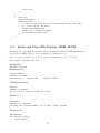
4.2.3 Field Data for Equations . . . . . . .
Mesh and Data File Format MSH ASCII . .
Output Files . . . . . . . . . . . . . . . . . .
4.4.1 Auxiliary Output Files . . . . . . . .
5 Main Input File Reference
.
.
.
.
.
.
.
.
.
.
.
.
.
.
.
.
.
.
.
.
.
.
.
.
.
.
.
.
.
.
.
.
.
.
.
.
.
.
.
.
.
.
.
.
.
.
.
.
.
.
.
.
.
.
.
.
.
.
.
.
.
.
.
.
.
.
.
.
.
.
.
.
.
.
.
.
.
.
.
.
.
.
.
.
.
.
.
.
.
.
.
.
.
.
.
.
.
.
.
.
.
.
.
.
.
.
.
.
.
.
.
.
.
.
.
.
.
.
.
.
.
.
.
.
.
.
.
.
47
47
47
48
49
50
51
53
55
4
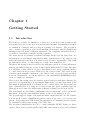
Chapter 1
Getting Started
1.1
Introduction
Flow123D is a software for simulation of water flow, reactionary solute transport and
heat transfer in a heterogeneous porous and fractured medium. In particular it is suited
for simulation of underground processes in a granite rock massive. The program is
able to describe explicitly processes in 3D medium, 2D fractures, and 1D channels and
exchange between domains of different dimensions. The computational mesh is therefore
a collection of tetrahedra, triangles and line segments.
The water flow model assumes a saturated medium described by the Darcy law. For
discretization, we use lumped mixed-hybrid finite element method. We support both
steady and unsteady water flow. The water flow model can be sequentially coupled with
two different models for a solute transport or with a heat transfer model.
The first solute transport model can deal only with pure advection of several substances
without any diffusion-dispersion term. It uses explicit Euler method for time discretization and finite volume method for space discretization and operator splitting method
to couple with various processes described by the reaction term. The reaction term
can treat any meaningful combination of the dual porosity, sorptions, decays and linear
reactions. Alternatively, one can use interface to the experimental SEMCHEM package
for more complex geochemistry.
The second solute transport model describes general advection with hydrodynamic dispersion for several substances. It uses implicit Euler method for time discretization and
discontinuous Galerkin method of the first, second or third order for the discretization in
space. Currently there is no support for reaction term, the operator splitting approach
(although it is not suited for implicit time schemes) is planned for the next version.
The heat transfer model assumes equilibrium between temperature of the rock and the
fluid phase. It uses the same numerical scheme as the second transport model.
The program support output of all input and many output fields into two file formats.
You can use file format of GMSH mesh generator and post-processor or you can use output into widely supported VTK format. In particular we recommend Paraview software
for visualization and post-processing of the VTK data.
The program is implemented in C/C++ using essentially PETSC library for linear
algebra. All models can run in parallel using MPI environment, however, the scalability
5
of the whole program is limited due to serial mesh and serial outputs.
The program is distributed under GNU GPL v. 3 license and is available on the project
web page: http://flow123d.github.io
with sources on the GitHub: https://github.com/flow123d/flow123d.
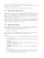
1.2
Reading Documentation
The Flow123d documentation has two main parts. The first three chapters form a user
manual which starts with getting and running the program and tutorial problem in
chapter 1. The second chapter 2 provides detailed description of mathematical models
of physical reality. The third chapter 4 documents all file types used by Flow123d,
including mesh files, input and output files.
The second main part, consisting only of the chapter 5, is automatically generated.
It mirrors directly the code and contains the whole input tree of the main input file.
Description of input records, their structure and default values are supplied there and
bidirectional links to the user manual are provided.
1.3
Running Flow123d
On the Linux system the program can be started either directly or through a script
flow123d.sh, both placed in the bin directory of the installation package or of the
source tree. When started directly, e.g. by the command
> flow123d -s example.con
the program requires one argument after switch -s which is the name of the principal
input file. Full list of possible command line arguments is as follows.
--help
Parameters interpreted by Flow123d. Remaining parameters are passed to PETSC.
-s, --solve <file>
Set principal CON input file. All relative paths in the CON file are relative against
current directory.
-i, --input dir <directory>
The placeholder ${INPUT} used in the path of an input file will be replaced by the
<directory>. Default value is input.
-o, --output dir <directory>
All paths for output files will be relative to this <directory>. Default value is
output.
-l, --log <file_name>
Set base name of log files. Default value is flow123d. The log files are individual
for every MPI process, placed in the output directory. The MPI rank of the process
and the log suffix are appended to the base name.
6
--no log
Turn off logging.
--no profiler
Turn off profiler output.
--full doc
Prints full structure of the main input file.
--latex doc
Prints a description of the main input file in LaTeX format using particular macros.
All other parameters will be passed to the PETSC library. An advanced user can
influence lot of parameters of linear solvers. In order to get list of supported options use
parameter -help together with some valid input. Options for various PETSC modules
are displayed when the module is used for the first time.
Alternatively, you can use script flow123d.sh to start parallel jobs or limit resources
used by the program. The syntax is as follows:
flow123d.sh [OPTIONS] -- [FLOW_PARAMS]
where everything after double dash is passed as parameters to the flow123d binary. The
script accepts following options:
-h, --help
Usage overview.
--host <hostname>
Default value is the host name obtained by system hostname command, this argument can be used to override it. Resulting value is used to select a backend
script config/<hostname>.sh, which describes particular method how to start
parallel jobs, usually through some sort of PBS job queue system. If the script is
not found, we try to start parallel processes directly on the actual host.”
-t, --walltime <timeout>
Upper estimate for real running time of the calculation. Kill calculation after
timeout seconds. Can also be used by PBS to choose appropriate job queue.
-np <number of processes>
Specify number of MPI parallel processes for calculation.
-m, --mem <memory limit>
Limits total available memory to <memory limit> bytes per process.
-n, --nice <niceness>
Change priority of the calculation, higher values means lower priority. See the
nice command.
-ppn <processes per node>
Set number of processes started on one node for multicore systems. Number of
processes set by -np parameter should be divisible by <processes per node>.
7
-q, --queue <queue>
Select particular job queue on PBS systems. If running without PBS, it redirects
stdout and stderr to the file <queue>.<date>, which appended date and time of
the start of the job.
On the windows operating systems, we use Cygwin libraries in order to emulate Linux
API. Therefore you have to keep the Cygwin libraries within the same directory as the
program executable. The Windows package that can be downloaded from project web
page contains both the Cygwin libraries and the mpiexec command for starting parallel
jobs on the windows based workstations.
Then you can start the sequential run by the command:
> flow123d.exe -s example.con
or the parallel run by the command:
> mpiexec.exe -np 2 flow123d.exe -s example.con
The program accepts the same parameters as the Linux version, but there is no script
similar to flow123d.sh for the windows operating systems.
1.4
Tutorial Problem
In the following section, we shall provide an example cook book for preparing and
running a model. It is one of the test problem with the main input file:
tests/03_transport_small_12d/flow_vtk.con
We shall start with preparation of the geometry using an external software and then
we shall go thoroughly through the commented main input file. The problem includes
steady Darcy flow, transport of two substances with explicit time discretization and a
reaction term consisting of dual porosity and sorption model.
1.4.1
Geometry
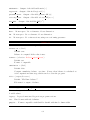
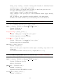
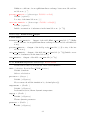
We consider a simple 2D problem with a branching 1D fracture (see Figure 1.1 for the
geometry). To prepare a mesh file we use the GMSH software. First, we construct
a geometry file. In our case the geometry consists of:
• one physical 2D domain corresponding to the whole square
• three 1D physical domains of the fracture
• four 1D boundary physical domains of the 2D domain
• three 0D boundary physical domains of the 1D domain
8
In this simple example, we can in fact combine physical domains in every group, however
we use this more complex setting for demonstration purposes. Using GMSH graphical
interface we can prepare the GEO file where physical domains are referenced by numbers,
then we use any text editor and replace numbers with string labels in such a way that
the labels of boundary physical domains start with the dot character. These are the
domains where we will not do any calculations but we will use them for setting boundary
conditions. Finally, we get the GEO file like this:
1
2
3
4
5
6
7
8
9
10
11
12
13
14
15
16
17
18
19
cl1 = 0.16;
Point(1) = {0, 1, 0, cl1};
Point(2) = {1, 1, 0, cl1};
Point(3) = {1, 0, 0, cl1};
Point(4) = {0, 0, 0, cl1};
Point(6) = {0.25, -0, 0, cl1};
Point(7) = {0, 0.25, 0, cl1};
Point(8) = {0.5, 0.5, -0, cl1};
Point(9) = {0.75, 1, 0, cl1};
Line(19) = {9, 8};
Line(20) = {7, 8};
Line(21) = {8, 6};
Line(22) = {2, 3};
Line(23) = {2, 9};
Line(24) = {9, 1};
Line(25) = {1, 7};
Line(26) = {7, 4};
Line(27) = {4, 6};
Line(28) = {6, 3};
Line Loop(30) = {20, -19, 24, 25};
Plane Surface(30) = {30};
Line Loop(32) = {23, 19, 21, 28, -22};
Plane Surface(32) = {32};
Line Loop(34) = {26, 27, -21, -20};
Plane Surface(34) = {34};
Physical Point(".1d_top") = {9};
Physical Point(".1d_left") = {7};
Physical Point(".1d_bottom") = {6};
Physical Line("1d_upper") = {19};
Physical Line("1d_lower") = {21};
Physical Line("1d_left_branch") = {20};
Physical Line(".2d_top") = {23, 24};
Physical Line(".2d_right") = {22};
Physical Line(".2d_bottom") = {27, 28};
Physical Line(".2d_left") = {25, 26};
Physical Surface("2d") = {30, 32, 34};
20
21
22
23
24
25
26
27
28
29
30
31
32
33
34
35
36
Notice the labeled physical domains on lines 26 – 36. Then we just set the discretization
step cl1 and use GMSH to create the mesh file. The mesh file contains both the ’bulk’
elements where we perform calculations and the ’boundary’ elements (on the boundary
physical domains) where we only set the boundary conditions.
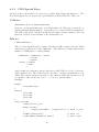
1.4.2
CON File Format
The main input file uses a slightly extended JSON file format which together with some
particular constructs forms a CON (C++ object notation) file format. Main extensions
of the JSON are unquoted key names (as long as they do not contain whitespaces),
possibility to use = instead of : and C++ comments, i.e. // for a one line and /* */
for a multi-line comment. In CON file format, we prefer to call JSON objects “records”
and we introduce also “abstract records” that mimic C++ abstract classes, arrays of a
CON file have only elements of the same type (possibly using abstract record types for
polymorphism). The usual keys are in lower case and without spaces (using underscores
instead), there are few special upper case keys that are interpreted by the reader: REF
key for references, TYPE key for specifing actual type of an abstract record. For detailed
description see Section 4.1.
Having the computational mesh from the previous step, we can create the main input
file with the description of our problem.
9
1
2
3
4
5
6
7
8
9
10
11
12
13
{
problem = {
TYPE = "SequentialCoupling",
description = "Tutorial problem:
Transport 1D-2D (convection, dual porosity, sorption, sources).",
mesh = {
mesh_file = "./input/mesh_with_boundary.msh",
sets = [
{ name="1d_domain",
region_labels = [ "1d_upper", "1d_lower", "1d_left_branch" ]
}
]
}, // mesh
The file starts with a selection of problem type (SequentialCoupling), and a textual
problem description. Next, we specify the computational mesh, here it consists of the
name of the mesh file and the declaration of one region set composed of all 1D regions
i.e. representing the whole fracture. Other keys of the mesh record allow labeling regions
given only by numbers, defining new regions in terms of element numbers (e.g to have
leakage on single element), defining boundary regions, and set operations with region
sets, see Section 4.2.1 for details.
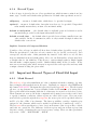
1.4.3
Flow Setting
Next, we setup the flow problem. We shall consider a flow driven only by the pressure
gradient (no gravity), setting the Dirichlet boundary condition on the whole boundary
with the pressure head equal to x + y. The conductivity will be k2 = 10−7 ms−1
on the 2D domain and k1 = 10−6 ms−1 on the 1D domain. Both 2D domain and 1D
domain cross section will be set by default, meaning that the thickness of 2D domain
is δ2 = 1 m and the fracture cross section is δ1 = 1 m2 . The transition coefficient σ2
between dimensions can be scaled by setting the dimensionless parameter σ21 (sigma).
This can be used for simulating additional effects which prevent the liquid transition
from/to a fracture, like a thin resistance layer. Read Section 2.3 for more details.
14
15
primary_equation = {
TYPE = "Steady_MH",
16
17
18
19
20
21
22
23
24
25
26
input_fields = [
{ r_set = "1d_domain", conductivity = 1e-6,
cross_section = 0.04,
sigma = 0.9 },
{ region = "2d",
conductivity = 1e-7 },
{ r_set = "BOUNDARY",
bc_type = "dirichlet",
bc_pressure = { TYPE="FieldFormula", value = "x+y" }
}
],
27
10
28
29
30
31
32
33
34
output = {
output_stream = {
file = "flow.pvd",
format = { TYPE = "vtk", variant = "ascii" }
},
output_fields = [ "pressure_p0", "pressure_p1", "velocity_p0" ]
},
35
36
37
38
39
40
41
solver = {
TYPE = "Petsc",
a_tol = 1e-12,
r_tol = 1e-12
}
}, // primary equation
On line 15, we specify particular implementation (numerical method) of the flow solver,
in this case the Mixed-Hybrid solver for steady problems. On lines 17 – 24, we set
both mathematical fields that live on the computational domain and those defining the
boundary conditions. We set only the conductivity field since other input fields have
appropriate default values. We use implicitly defined set “BOUNDARY” that contains
all boundary regions and set there dirichlet boundary condition in terms of the pressure
head. In this case, the field is not of the implicit type FieldConstant, so we must
specify the type of the field TYPE="FieldFormula". See Section 4.2.2 for other field
types. On lines 26 – 32, we specify which output fields should be written to the output
stream (that means particular output file, with given format). Currently, we support
only one output stream per equation, so this allows at least switching individual output
fields on or off. See Section 4.4 for the list of available output fields. Finally, we
specify type of the linear solver and its tolerances.
1.4.4
Transport Setting
The flow model is followed by a transport model in the secondary equation beginning
on line 40. For the transport problem, we use an implementation called TransportOperatorSplitting which stands for an explicit finite volume solver of the convection equation
(without diffusion). The operator splitting method is used for equilibrium sorption as
well as for dual porosity model and first order reactions simulation.
42
43
secondary_equation = {
TYPE = "TransportOperatorSplitting",
44
45
46
47
48
substances = [
{name = "age", molar_mass = 0.018},
{name = "U235", molar_mass = 0.235}
],
49
50
51
52
input_fields= [
{ r_set = "ALL",
init_conc = 0,
11
// water age
// uranium 235
porosity= 0.25,
sources_density = [1.0, 0]
},
{ r_set = "BOUNDARY",
bc_conc = [0.0, 1.0]
}
],
53
54
55
56
57
58
59
60
time = { end_time = 1e6 },
mass_balance = { cumulative = true },
61
62
On lines 43 – 46, we set the transported substances, which are identified by their
names. Here, the first one is the age of the water, with the molar mass of water, and
the second one U235 is the uranium isotope 235. On lines 48 – 57, we set the input
fields, in particular zero initial concentration for all substances, porosity θ = 0.25 and
sources of concentration by sources density. Notice line 50 where we can see only
single value since an automatic conversion is applied to turn the scalar zero into the
zero vector (of size 2 according to the number of substances).
The boundary fields are set on lines 54 – 56. We need not to specify the type of the
condition since there is only one type in the current transport model. The boundary
condition is equal to 1 for the uranium 235 and 0 for the age of the water and is
automatically applied only on the inflow part of the boundary.
We also have to prescribe the time setting, here only the end time of the simulation (in
seconds: 106 s ≈ 11.57 days) is required since the step size is determined from the CFL
condition. However, a smaller time step can be enforced if necessary.
Reaction term of the transport model is described in the next subsection, including dual
porosity and sorption.
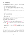
1.4.5
Reaction Term
The input information for dual porosity, equilibrial sorption and possibly first order
reations are enclosed in the record reaction term, lines 61 – 100. Go to section 2.5 to
see how the models can be chained.
The type of the first process is determined by TYPE="DualPorosity", on line 62. The
input fields of dual porosity model are set on lines 64 – 71 and the output is disabled
by setting an empty array on line 73.
63
64
reaction_term = {
TYPE = "DualPorosity",
65
66
67
68
69
70
71
input_fields= [
{
r_set="ALL",
diffusion_rate_immobile = [0.01,0.01],
porosity_immobile = 0.25,
init_conc_immobile = [0.0, 0.0]
12
}
],
72
73
74
output_fields = [],
75
76
reaction_mobile = {
TYPE = "SorptionMobile",
solvent_density = 1000.0,
// water
substances = ["age", "U235"],
solubility = [1.0, 1.0],
77
78
79
80
81
82
input_fields= [
{
r_set="ALL",
rock_density = 2800.0,
// granit
sorption_type = ["none", "freundlich"],
isotherm_mult = [0, 0.68],
isotherm_other = [0, 1.0]
}
],
output_fields = []
},
reaction_immobile = {
TYPE = "SorptionImmobile",
solvent_density = 1000.0,
// water
substances = ["age", "U235"],
solubility = [1.0, 1.0],
input_fields = { REF="../../reaction_mobile/input_fields" },
output_fields = []
}
},
83
84
85
86
87
88
89
90
91
92
93
94
95
96
97
98
99
100
101
102
103
output_stream = {
file = "transport.pvd",
format = { TYPE = "vtk", variant = "ascii" },
time_step = 1e5
}
104
105
106
107
108
109
} // secondary_equation
} // problem
110
111
112
}
Next, we define the equilibrial sorption model such that SorptionMobile type takes
place in the mobile zone of the dual porosity model while SorptionImmobile type
takes place in its immobile zone, see lines 76 and 93. Isothermally described sorption
simulation can be used in the case of low concentrated solutions without competition
between multiple dissolved species.
On lines 77 – 89, we set the sorption related input information. The solvent is water so
13
the solvent density is supposed to be constant all over the simulated area. The vector
substances contains the list of names of soluted substances which are considered to be
affected by the sorption. Solubility is a material characteristic of a sorbing substance
related to the solvent. Elements of the vector solubility define the upper bound of
aqueous concentration which can appear. This constrain is necessary because some
substances might have limited solubility and if the solubility exceeds its limit they start
to precipitate. solubility is a crucial parameter for solving a set of nonlinear equations,
described further.
The record input fields covers the region specific parameters. All implemented types
of sorption can take the rock density in the region into account. The value of rock density
is a constant in our case. The sorption type represents the empirically determined
isotherm type and can have one of four possible values: {"none", "linear", "freundlich",
"langmuir"}. Linear isotherm needs just one parameter given whereas Freundlichs’ and
Langmuirs’ isotherms require two parameters. We will use Freundlich’s isotherm for
demonstration but we will set the other parameter (exponent) α = 1 which means it
will be the same as the linear type.
Let suppose we have a sorption coefficient for uranium Kd = 1.6·10−4 kg−1 m3 (www.skb.se,
report R-10-48 by James Crawford, 2010) and we want to use. We need to convert it to
1000
≈
dimensionless value of isotherm mult in the following way: kl = Kd Ms−1 ρl = Kd 0.235
0.68. For further details, see mathematical description in Section 2.5.2.
On line 97, notice the reference pointing to the definition of input fields on lines 81 –
89. Only entire records can be referenced which is why we have to repeat parts of the
input such as solvent density and solubility (records for reaction mobile and reaction
immobile have different types).
On lines 90 and 98, we define which sorption specific outputs are to be written to the
output file. An implicit set of outputs exists. In this case we define an empty set of
outputs thus overriding the implicit one. This means that no sorption specific outputs
will be written to the output file. On lines 102 – 106 we specify which output fields
should be written to the output stream. Currently, we support output into VTK and
GMSH data format. In the output record for time-dependent process we have to specify
the time step (line 105) which determines the frequency of saving.
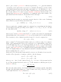
1.4.6
Results
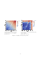
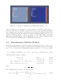
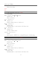
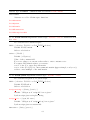
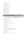
In Figure 1.1 one can see the results: the pressure and the velocity field on the left
and the concentration of U235 at time t = 9 · 105 s on the right. Even if the pressure
gradient is the same in the 2D domain and in the fracture, due to higher conductivity
the velocity field is ten times faster in the fracture. Since porosity is the same, the
substance is transported faster by the fracture and then appears in the bottom left 2D
domain before the main wave propagating solely through the 2D domain.
In the following chapter we describe mathematical models used in Flow123d. Then in
chapter 4 we briefly describe structure of individual input files, in particular the main
CON file. The complete description of the CON format is given in chapter 5.
14
1.89
pressure head
1.00
1.60
0.80
1.20
0.60
0.80
0.40
0.40
0.20
0.09
(a) Elementwise pressure head and
velocity field denoted by triangles.
(Steady flow.)
concentration
0.01
(b) Propagation of U235 from the inflow part
of the boundary.
(At the time 9 · 105 s.)
Figure 1.1: Results of the tutorial problem.
15
Chapter 2
Mathematical Models
of Physical Reality
Flow123d provides models for Darcy flow in porous media as well as for the transport
and reactions of solutes. In this section, we describe mathematical formulations of these
models together with physical meaning and units of all involved quantities. In the first
section we present basic notation and assumptions about computational domains and
meshes that combine different dimensions. In the next section we derive approximation
of thin fractures by lower dimensional interfaces for a general transport process. Latter
sections describe details for models of particular physical processes.
2.1
Meshes of Mixed Dimension
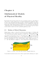
Unique feature common to all models in Flow123d is the support of domains with
mixed dimension. Let Ω3 ⊂ R3 be an open set representing continuous approximation
of porous and fractured medium. Similarly, we consider a set of 2D manifolds Ω2 ⊂ Ω3 ,
representing the 2D fractures and a set of 1D manifolds Ω1 ⊂ Ω2 representing the 1D
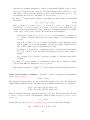
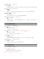
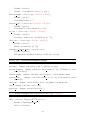
channels or preferential paths (see Fig 2.1). We assume that Ω2 and Ω1 are polytopic
(i.e. polygonal and piecewise linear, respectively). For every dimension d = 1, 2, 3, we
introduce a triangulation Td of the open set Ωd that consists of finite elements Tdi , i =
1, . . . , NEd . The elements are simplices, i.e. lines, triangles and tetrahedra, respectively.
Figure 2.1: Scheme of a problem with domains of multiple dimensions.
Present numerical methods used by the software require meshes satisfying the compat16
ibility conditions
i
Td−1
∩ Td ⊂ Fd ,
where Fd =
[
∂Tdk
(2.1)
k
and
i
i
or ∅
∩ Fd is either Td−1
Td−1
(2.2)
for every i ∈ {1, . . . , NEd−1 }, j ∈ {1, . . . , NEd }, and d = 2, 3. That is, the (d − 1)dimensional elements are either between d-dimensional elements and match their sides
or they poke out of Ωd . Support for a coupling between non-compatible meshes of
different dimesion is in developement and partly supported by the Darcy Flow model.
2.2
Advection-Diffusion Processes on Fractures
This section presents derivation of an abstract advection-diffusion process on 2D and
1D manifolds and its coupling with the higher dimensional domains. The reader not
interested in the details of this approximation may skip directly to the later sections
describing mathematical models of individual physical processes.
As was already mentioned, the unique feature of Flow123d is support of models living
on 2D and 1D manifolds. The aim is to capture features significantly influencing the
solution despite of their small cross-section. Such a tiny features are challenging for
numerical simulations since a direct discretization requires highly refined computational
mesh. One possible solution is to model these features (fractures, channels) as lower
dimensional objects (2D and 1D manifolds) and introduce their coupling with the surrounding continuum. The equations modeling a physical process on a manifold as well
as its coupling to the model in the surrounding continuum has to be derived from the
model on the 3D continuum. This section presents such a procedure for the case of the
abstract advection-diffusion process inspired by the paper [7]. Later, we this abstract
approach to particular advection-diffusion processes: Darcian flow, solute transport, and
heat transfer.
Let us consider a fracture as a strip domain
Ωf ⊂ [0, δ] × Rd−1
for d = 2 or d = 3 and surrounding continuum domains
Ω1 ⊂ (−∞, 0) × Rd−1 , Ω2 ⊂ (δ, ∞) × Rd−1 .
Further, we denote by γi , i = 1, 2 the fracture faces common with domains Ω1 and Ω2
respectively. By x, y we denote normal and tangential coordinate of a point in Ωf . We
consider the normal vector n = n1 = −n2 = (1, 0, 0)> . An advection-diffusion process
is given by equations:
∂t wi + divj i = fi
j i = −Ai ∇ui + bi wi
ui = uf
ji · n = jf · n
on
on
on
on
Ωi , i = 1, 2, f,
Ωi , i = 1, 2, f,
γi , i = 1, 2,
γi , i = 1, 2,
(2.3)
(2.4)
(2.5)
(2.6)
where wi = wi (ui ) is the conservative quantity and ui is the principal unknown, j i is
the flux of wi , fi is the source term, Ai is the diffusivity tensor and bi is the velocity
17
field. We assume that the tensor Af is symmetric positive definite with one eigenvector
in the direction n. Consequently the tensor has the form:
an 0
Af =
0 At
Furthermore, we assume that Af (x, y) = Af (y) is constant in the normal direction.
Our next aim is to integrate equations on the fracture Ωf in the normal direction and
obtain their approximations on the surface γ = Ωf ∩ {x = δ/2} running through the
middle of the fracture. For the sake of clarity, we will not write subscript f for quantities
on the fracture. To make the following procedure mathematicaly correct we have to
assume that functions ∂x w, ∂x ∇y u, ∂x by are continuous and bounded on Ωf . Here and
later on bx = (b · n) n is the normal part of the velocity field and by = b − bx is the
tangential part. The same notation will be used for normal and tangential part of the
field q.
We integrate (2.3) over the fracture opening [0, δ] and use approximations to get
∂t (δW ) − j 2 · n2 − j 1 · n1 + divJ = δF,
(2.7)
where for the first term, we have used mean value theorem, first order Taylor expansion,
and boundedness of ∂x w to obtain approximation:
Z δ
w(x, y) dx = δw(ξy , y) = δW (y) + O(δ 2 |∂x w|),
0
where
W (y) = w(δ/2, y) = w(u(δ/2, y)) = w(U (y)).
Next two terms in (2.7) come from the exact integration of the divergence of the normal
flux j x . Integration of the divergence of the tangential flux j y gives the fourth term,
where we introduced
Z δ
j y (x, y) dx.
J (y) =
0
In fact, this flux on γ is scalar for the case d = 2. Finally, we integrate the right-hand
side to get
Z δ
f (x, y) dx = δF (y) + O(δ 2 |∂x f |), F (y) = f (δ/2, y).
0
Due to the particular form of the tensor Af , we can separately integrate tangential
and normal part of the flux given by (2.4). Integrating the tangential part and using
approximations
Z δ
∇y u(x, y) dx = δ∇y u(ξy , y) = δ∇y U (y) + O δ 2 |∂x ∇y u|
0
and
Z
δ
by w (x, y) dx = δB(y)W (y) + O δ 2 |∂x (by w)|
0
where
B(y) = by (δ/2, y),
18
we obtain
J = −At δ∇y U + δBW + O δ 2 (|∂x ∇y u| + |∂x (by w)|) .
(2.8)
So far, we have derived equations for the state quantities U and J on the fracture
manifold γ. In order to get a well possed problem, we have to prescribe two conditions
for boundaries γi , i = 1, 2. To this end, we perform integration of the normal flux j x ,
given by (2.4), separately for the left and right half of the fracture. Similarly as before
we use approximations
Z δ/2
δ
j x dx = (j 1 · n1 ) + O(δ 2 |∂x j x |)
2
0
and
Z
0
δ/2
δ
bx w dx = (b1 · n1 )w̃1 + O(δ 2 |∂x bx ||w| + δ 2 |bx ||∂x w|)
2
and their counter parts on the interval (δ/2, δ) to get
2an
(U − u1 ) + b1 · n1 w̃1
δ
2an
j 2 · n2 = −
(U − u2 ) + b2 · n2 w̃2
δ
j 1 · n1 = −
(2.9)
(2.10)
where w̃i can be any convex combination of wi and W . Equations (2.9) and (2.10) have
meaning of a semi-discretized flux from domains Ωi into fracture. In order to get a
stable numerical scheme, we introduce a kind of upwind already on this level using a
different convex combination for each flow direction:
j i · ni = − σi (U − ui )
+
+ bi · ni
ξwi + (1 − ξ)W
−
+ bi · ni
(1 − ξ)wi + ξW ,
i = 1, 2
(2.11)
where σi = 2aδn is the transition coefficient and the parameter ξ ∈ [ 12 , 1] can be used to
interpolate between upwind (ξ = 1) and central difference (ξ = 21 ) scheme. Equations
(2.7), (2.8), and (2.11) describe the general form of the advection-diffusion process on
the fracture and its communication with the surrounding continuum which we shall later
apply to individual processes.
2.3
Darcy Flow Model
We consider the simplest model for the velocity of the steady or unsteady flow in porous
and fractured medium given by the Darcy flow:
w = −K∇H
in Ωd , for d = 1, 2, 3.
(2.12)
Here and later on, we drop the dimension index d of the quantities if it can be deduced
from the context. In (2.12), w [ms−1 ] is the superficial velocity, Kd is the conductivity
tensor, and H [m] is the piezometric head. The velocity wd is related to the flux q d
[m4−d s−1 ] through
q d = δd wd ,
19
where δd [m3−d ] is the cross section coefficient, in particular δ3 = 1, δ2 [m] is the thickness
of a fracture, and δ1 [m2 ] is the cross-section of a channel. The flux q d · n is the volume
of the liquid (water) that passes through a unit square (d = 3), unit line (d = 2), or
through a point (d = 1) per one second. The conductivity tensor is given by the product
Kd = kd Ad , where kd > 0 [ms−1 ] is the hydraulic conductivity and Ad is the 3 × 3
dimensionless anisotropy tensor which has to be symmetric and positive definite. The
piezometric-head Hd is related to the pressure head hd through
Hd = hd + z
(2.13)
assuming that the gravity force acts in the negative direction of the z-axis. Combining
these relations, we get the Darcy law in the form:
q = −δkA∇(h + z)
in Ωd , for d = 1, 2, 3.
(2.14)
Next, we employ the continuity equation for saturated porous medium and the dimensional reduction from the preceding section (with w = u := H, j := w, A := K and
b := 0), which yields:
∂t (δS h) + divq = F
in Ωd , for d = 1, 2, 3,
(2.15)
where Sd [m−1 ] is the storativity and Fd [m3−d s−1 ] is the source term. In our setting the
principal unknowns of the system (2.14, 2.15) are the pressure head hd and the flux q d .
The storativity (or the volumetric specific storage) Sd > 0 can be expressed as
Sd = γw (βr + ϑβw ),
(2.16)
where γw [kgm−2 s−2 ] is the specific weight of water, ϑ [−] is the porosity, βr is compressibility of the bulk material of the pores (rock) and βw is compressibility of the water,
both with units [kg−1 ms−2 ]. For steady problems, we set Sd = 0 for all dimensions
d = 1, 2, 3. The source term Fd on the right hand side of (2.15) consists of the volume
density of the water source fd [s−1 ] and flux from the from the higher dimension. Precise
form of Fd slightly differs for every dimension and will be discussed presently.
In Ω3 we simply have F3 = f3 [s−1 ].
In the set Ω2 ∩ Ω3 the fracture is surrounded by at most one 3D surface from every side.
On ∂Ω3 ∩ Ω2 we prescribe a boundary condition of the Robin type:
+
q 3 · n+ = q32
= σ3 (h+
3 − h2 ),
−
−
q 3 · n = q32 = σ3 (h−
3 − h2 ),
+/−
where q 3 · n+/− [ms−1 ] is the outflow from Ω3 , h3
is a trace of the pressure head in
−1
Ω3 , h2 is the pressure head in Ω2 , and σ3 [s ] is the transition coefficient given by (see
section 2.2 and [7])
2K2 : n2 ⊗ n2
.
σ3 = σ32
δ2
Here n2 is the unit normal to the fracture (sign does not matter). On the other hand,
+/−
the sum of the interchange fluxes q32 forms a volume source in Ω2 . Therefore F2 [ms−1 ]
on the right hand side of (2.15) is given by
+
−
).
F2 = δ2 f2 + (q32
+ q32
20
(2.17)
The communication between Ω2 and Ω1 is similar. However, in the 3D ambient space,
a 1D channel can join multiple 2D fractures 1, . . . , n. Therefore, we have n independent
outflows from Ω2 :
i
= σ2 (hi2 − h1 ),
q 2 · ni = q21
where σ2 [ms−1 ] is the transition coefficient integrated over the width of the fracture i:
σ2 = σ21
2δ22 K1 : ni1 ⊗ ni1
.
δ1
Here ni1 is the unit normal to the channel that is tangential to the fracture i. Sum of
the fluxes forms a part of F1 [m2 s−1 ]:
F 1 = δ1 f 1 +
n
X
i
q21
.
(2.18)
i=1
We remark that the direct communication between 3D and 1D (e.g. model of a well) is
not supported yet. The transition coefficients σ32 [−] and σ21 [−] are independent scaling
parameters which represent the ratio of the crosswind and the tangential conductivity
in the fracture. For example, in the case of impermeable film on the fracture walls one
may choice σ32 < 1.
In order to obtain unique solution we have to prescribe boundary conditions. Currently
we support three basic types of boundary conditions:
Dirichlet boundary condition
D
hd = hD
d on Γd ,
where hD
d [m] is the boundary pressure head . Alternatively one can prescribe the
boundary piezometric head HdD [m] related to the pressure head through (2.13).
Neuman boundary condition
q d · n = qdN on ΓN
d ,
where qdN [m4−d s−1 ] is the surface density of the water outflow.
Robin boundary condition
R
q d · n = σdR (hd − hR
d ) on Γd .
R
3−d −1
where hR
s ] is the transition coefficient.
d is the boundary pressure head and σd [m
As before one can also prescribe the boundary piezo head HdR to specify hR
d.
We consider a disjoint decomposition of the boundary
R
∂Ωd = ∩ΓN
d ∩ Γd
into Dirichlet, Neumann, and Robin part. In order to obtain well posed steady state
problem one have to prescribe Dirichlet or Robin boundary condition on part of boundary that is connected (geometricaly of through the inter dimensional coupling) to hte
rest of the domain.
For unsteady problems one has to specify an initial condition in terms of the initial
pressure head h0d [m] or the initial piezometric head Hd0 [m].
21
Volume balance. The equation (2.15) satisfies the volume balance of the liquid in
the following form:
Z t
Z t
V (0) +
s(τ ) dτ −
f (τ ) dτ = V (t)
0
0
for any instant t in the computational time interval. Here
V (t) :=
3 Z
X
s(t) :=
(δSh)(t, x) dx,
Ωd
d=1
3 Z
X
f (t) :=
3 Z
X
d=1
F (t, x) dx,
Ωd
d=1
q(t, x) · n(x) dx
∂Ωd
is the volume [m3 ], the volume source [m3 s−1 ] and the volume flux [m3 s−1 ] of the liquid
at time t, respectively. The volume, flux and source on every geometrical region is
calculated at each computational time step and the values together with the control
sums are written to the file water balance.txt.
2.4
Transport of Substances
The motion of substances dissolved in water is governed by the advection, and the
hydrodynamic dispersion. In Ωd , d ∈ {1, 2, 3}, we consider the following system of mass
balance equations1 :
∂t (δϑci ) + div(qci ) − div(ϑδDi ∇ci ) = FSi + FCc + FR (c1 , . . . , cs ).
(2.19)
The principal unknown is the concentration ci [kgm−3 ] of a substance i ∈ {1, . . . , s},
which means the weight of the substance in the unit volume of water. Other quantities
are:
• The porosity ϑ [−], i.e. the fraction of space occupied by water and the total
volume.
• The hydrodynamic dispersivity tensor Di [m2 s−1 ] has the form
i
i
i
i
i v⊗v
,
D = Dm τ I + |v| αT I + (αL − αT )
|v|2
(2.20)
which represents (isotropic) molecular diffusion, and mechanical dispersion in loni
gitudal and transversal direction to the flow. Here Dm
[m2 s−1 ] is the molecular
diffusion coefficient of the i-th substance (usual magnitude in clear water is 10−9 ),
τ = ϑ1/3 is the tortuosity (by [8]), αLi [m] and αTi [m] is the longitudal dispersivity and the transverse dispersivity, respectively. Note that although we allow
dispersivities to have different values for different substances, it is often assumed
1
For d ∈ {1, 2} this form can be derived as in Section 2.2 using w := δϑci , u := ci , A := δϑDi ,
q
b := v = ϑδ
.
22
that they are intrinsic parameters of the porous medium. Finally, v [ms−1 ] is the
microscopic water velocity, related to the Darcy flux q by the relation q = ϑδv.
i
The value of Dm
for specific substances can be found in literature (see e.g. [2]).
For instructions on how to determine αLi , αTi we refer to [3, 4].
• FSi [kgm−d s−1 ] represents the density of concentration sources in the porous medium.
Its form is:
(2.21)
FSi = δfSi + δ(ciS − ci )σSi .
Here fSi [kgm−3 s−1 ] is the density of concentration sources, ciS [kgm−3 ] is an
equilibrium concentration and σSi [s−1 ] is the concentration flux. One has to pay
attention when prescribing the source, namely to determine whether it is related
to the liquid or the porous medium. We mention several examples:
– extraction of solution: fSi = 0, ciS = 0, σSi > 0 is the intensity of extraction,
i.e. volume of liquid extracted from a unit volume of porous medium per
second;
– injection of solution: fSi = 0, ciS is the concentration of the substance in the
injected liquid, σSi > 0 is the intensity of injection (volume of liquid injected
into a unit volume of porous medium per second);
– production or degradation of substances due to bacteria present in liquid:
fSi = ϑpi , where pi is the production/degradation rate in a unit volume of
liquid;
– age of liquid: if fSi = ϑ then ci is the age of liquid, i.e. the time spent in the
domain.
• FCc [kgm−d s−1 ] is the density of concentration sources due to exchange between
regions with different dimensions, see (2.23) below.
• The reaction term FR (. . . ) [kgm−d s−1 ] is thoroughly described in the next section
2.5.
Initial and boundary conditions. At time t = 0 the concentration is determined
by the initial condition
ci (0, x) = ci0 (x).
The physical boundary ∂Ωd is decomposed into the parts ΓI ∪ ΓD ∪ ΓN ∪ ΓR , which may
change during simulation time. The first part ΓI is further divided into two segments:
Γ+
I (t) = {x ∈ ∂Ωd | q(t, x) · n(x) < 0},
−
ΓI (t) = {x ∈ ∂Ωd | q(t, x) · n(x) ≥ 0},
where n stands for the unit outward normal vector to ∂Ωd . We prescribe the following
boundary conditions: On ΓD , the Dirichlet condition is imposed via prescribed concentration ciD :
ci = ciD on ΓD .
i
On the inflow Γ+
I the reference concentration cD is enforced through total flux:
(qci − ϑδDi ∇ci ) · n = q · nciD on Γ+
I ,
23
on Γ−
I we impose homogeneous Neumann condition:
−ϑδDi ∇ci · n = 0 on Γ−
I ,
on ΓN we impose Neumann condition with user-defined concentration flux fNi :
−ϑδDi ∇ci · n = fNi on ΓN ,
and finally on ΓR we impose Robin condition through transition parameter σRi and
reference concentration ciD :
−ϑδDi ∇ci · n = σRi (ci − ciD ) on ΓR .
Communication between dimensions. Transport of substances is considered also
on interfaces of physical domains with adjacent dimensions (i.e. 3D-2D and 2D-1D, but
not 3D-1D). Denoting cd+1 , cd the concentration of a given substance in Ωd+1 and Ωd ,
respectively, the comunication on the interface between Ωd+1 and Ωd is described by the
quantity
(
l
2
ql
cd+1
if qd+1,d
≥ 0,
δ
d+1
c
c
2ϑd Dd : n ⊗ n(cd+1 − cd ) + d+1,d
(2.22)
qd+1,d
= σd+1,d
ϑd
l
l
δd
qd+1,d ϑd+1 cd if qd+1,d < 0,
where
c
• qd+1,d
[kgm−d s−1 ] is the density of concentration flux from Ωd+1 to Ωd ,
c
• σd+1,d
[−] is a transition parameter. Its value determines the mass exchange between dimensions whenever the concentrations differ. In general, it is recommended to leave the default value σ c = 1 or to set σ c = 0 (when exchange is due
to water flux only).
l
l
• qd+1,d
[m3−d s−1 ] is the water flux from Ωd+1 to Ωd , i.e. qd+1,d
= q d+1 · nd+1 .
The communication between dimensions is incorporated as the total flux boundary condition for the problem on Ωd+1 :
−ϑδD∇c · n + q l c = q c
(2.23)
and a source term in Ωd :
c
FC3
= 0,
c
c
FC2
= q32
,
c
c
FC1
= q21
.
(2.24)
Mass balance. The advection-dispersion equation satisfies the balance of mass in the
following form:
Z
Z
t
mi (0) +
t
si (τ ) dτ −
0
f i (τ ) dτ = mi (t)
0
for any instant t in the computational time interval and any substance i. Here
i
m (t) :=
3 Z
X
d=1
(δϑci )(t, x) dx,
Ωd
24
i
s (t) :=
3 Z
X
d=1
f i (t) :=
3 Z
X
d=1
Ωd
FSi (t, x) dx,
qci − ϑδDi ∇ci (t, x) · n dx
∂Ωd
is the mass [kg], the volume source [kgs−1 ] and the mass flux [kgs−1 ] of i-th substance at
time t, respectively. The mass, flux and source on every geometrical region is calculated
at each computational time step and the values together with the control sums are
written to the file mass balance.txt.
Two transport models. Within the above presented model, Flow123d presents two
possible approaches to solute transport.
• For modelling pure advection (D = 0) one can choose TransportOperatorSplitting
method, which represents an explicit in time finite volume solver. Only the inflow/outflow boundary condition is available and the source term has the form
FSi = δfSi + δ(ciS − ci )+ σSi .
The solution process for one time step is faster, but the maximal time step is restricted. The resulting concentration is piecewise constant on mesh elements. This
solver supports reaction term (involving simple chemical reactions, dual porosity
and sorption).
• The full model including dispersion is solved by SoluteTransport DG, an implicit
in time discontinuous Galerkin solver. It has no restriction of the computational
time step and the space approximation is piecewise polynomial, currently up to
order 3. Reaction term is currently not implemented.
2.5
Reaction Term in Transport
The TransportOperatorSplitting method supports the reaction term FR (c1 , . . . , cs )
on the right hand side of the equation (2.19). It can represent several models of chemical
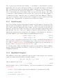
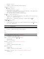
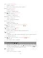
or physical nature. Figure 2.2 shows all possible reactional models that we support
in combination with the transport process. The Operator Splitting method enables
us to deal with the convection part and reaction term side by side. The convected
quantities do not influence each other in the convectional process and are balanced over
the elements. On the other hand the reaction term relates the convected quantities and
can be computed separately on each element.
We move now to the description of the reaction models which can be seen again in
Figure 2.2. The convected quantity is considered to be the concentration of substances.
Up to now we can have dual porosity, sorption (these two are more of a physical nature)
and (chemical) reaction models in the reaction term.
The reaction model acts only on the specified substances and computes exchange of
concentration among them. It does not have its own output because it only changes the
concentration of substances in the specified zone where the reaction takes place.
25
Operator Splitting
Transport process
Reaction term
- independent substances
- independent elements (dofs)
Dual Porosity
Sorption
Reaction
Dual Porosity
Mobile
Immobile
Sorption
Sorption
Reaction
Reaction
Sorption
Liquid
Reaction
Solid
Reaction
Decay
...
Reaction
Figure 2.2: The scheme of the reaction term objects. The lines represents connections
between different models. The tables under model name include the possible models
which can be connected to the model above.
26
The sorption model describes the exchange of concentration of the substances between
liquid and solid. It can be followed by another reaction that can run in both phases.
The concentration in solid is an additional output of this model. See Subsection 2.5.2.
The dual porosity model, described in Subsection 2.5.1, introduces the so called immobile (or dead-end) pores in the matrix. The convection process operates only on the
concentration of the substances in the mobile zone (open pores) and the exchange of
concentrations from/to immobile zone is governed by molecular diffusion. This process can be followed by sorption model and/or chemical reaction, both in mobile and
immobile zone. The immobile concentration is an additional output.
2.5.1
Dual Porosity
Up to now, we have described the transport equation for the single porosity model. The
dual porosity model splits the mass into two zones – the mobile zone and the immobile
zone. Both occupy the same macroscopic volume, however on the microscopic scale, the
immobile zone is formed by the dead-end pores, where the liquid is trapped and cannot
pass through. The rest of the pore volume is occupied by the mobile zone. Since the
liquid in the immobile pores is immobile, the exchange of the substance is only due to
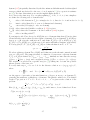
molecular diffusion. We consider simple nonequilibrium linear model:
ϑm ∂t cm = Ddp (ci − cm ),
ϑi ∂t ci = Ddp (cm − ci ),
(2.25a)
(2.25b)
where cm is the concentration in the mobile zone, ci is the concentration in the immobile
zone and Ddp is a diffusion rate between the zones. ϑi denotes porosity of the immobile
zone and ϑm = ϑ the mobile porosity from transport equation (2.19). One can also set
non-zero initial concentration in the immobile zone ci (0).
To solve the system of first order differential equation, we use analytic solution or Euler’s
method, which are switched according to a given error tolerance. See subsection 3.4.1
in numerical methods.
2.5.2
Equilibrial Sorption
The simulation of monolayer, equilibrial sorption is based on the solution of two algebraic
equations, namely the mass balance (in unit volume)
ϑ%l cl + (1 − ϑ)%s Ms cs = cT = const.
(2.26)
and an empirical sorption law
cs = f (cl ),
(2.27)
given in terms of the so-called isotherm f . Its form is determined by the parameter
sorption type:
• “none”: f (cl ) = 0 (the sorption model returns zero concentration in solid);
• “linear”: f (cl ) = kl cl ;
• “f reundlich”: f (cl ) = kF cαl ;
27
αcl
• “langmuir”: f (cl ) = kL 1+αc
. Langmuir isotherm has been derived from thermol
dynamic laws. kL denotes the maximal amount of sorbing specie which can be
kept in an unit volume of a bulk matrix. Coefficient α is a fraction of sorption
and desorption rate constant α = kkad .
Notation:
• In solid, cs = mns [mol kg−1 ] is the fraction of the molar amount of the solute
adsorbed n and the amount of the adsorbent ms (mass of solid), all in unit volume.
The concentration in solid can be selected for output.
m
• In liquid, cl = m
[−] is the fraction of the amount of the solute m and the mass
l
of liquid ml , all in unit volume. The relation between cl and the concentration c
from transport equation (2.19) is c = cl %l .
• %l , %s is the liquid (solvent) density and the solid (rock) density, respectively.
• Ms denotes the molar mass of a substance.
• Multiplication parameters are ki , i ∈ {l, F, L} [mol kg−1 ].
• Additional parameter [α] = 1 can be set.
Non-zero initial concentration in the solid phase cs (0) can be set in the input record.
Now, further denoting
µl = %l ϑ, µs = Ms %s · (1 − ϑ),
and using (2.27), the mass balance (2.26) reduces to the equation
cT = µl cl + µs f (cl ),
(2.28)
which can be either solved iteratively or using interpolation. See subsection 3.4.2 in
numerical methods for details.
The units of cl , cs and ki can vary in literature. To avoid misinterpretation, we derive
(according to Bowman [1]) a conversion rule for Freundlich isotherm which will lead the
user also in other cases, we believe.
Units conversion. Let us have c [kgm−3 ], the mass concentration in liquid, and
s [kg kg−1 ], the fraction of the amount of the solute adsorbed and the amount of the
adsorbent in solid. The unit of K follows from the dimensional analysis of s = Kcα :
[K] =
kg1−α m3α
,
kg
which we want to convert to kF [mol kg−1 ] in the formula cs = kF cαl .
The first step is a conversion of the mass of the solute to moles by dividing it by the
molar mass Ms . We then have the formula
α
s = Kc
α
s
c
0
= K
,
Ms
Ms
s = K 0 Ms1−α cα ,
28
(2.29)
where s = cs Ms and K 0 = KMsα−1 [mol1−α kg−1 m3α ] is a new constant, distributing the
molar concentration in liquid to the ratio of the molar mass and the amount of sorbent
in solid.
The second step is introducing cl =
cs = K
0
cl ρ l
Ms
α
c
%l
into the formula (2.29)
= K 0 Ms−α ραl cαl = KMs−1 ραl cαl ,
(2.30)
kF = KMs−1 ραl ,
(2.31)
where we can denote
which is the constant we are looking for. This can be also translated to the case of the
linear isotherm, where α = 1 and [K] = kg−1 m3 , and we get the conversion rule
kl = KMs−1 ρl .
(2.32)
The conversion of different prefixes of units are left on the user. One should be careful
using the Freundlich isotherm, though, where the exponent α must not be forgotten.
2.5.3
Sorption in Dual Porosity Model
There are two parameters µl and µs , scale of aqueous concentration and scale of sorbed
concentration, respectively. There is a difference in computation of these in the dual
porosity model because both work on different concentrations and different zones.
Let cml and cms be concentration in liquid and in solid in the mobile zone, cil and cis be
concentration in liquid and in solid in the immobile zone, ϑm and ϑi be the mobile and
the immobile porosity, and ϕ be the sorbing surface.
The sorbing surface in the mobile zone is given by
ϕ=
ϑm
,
ϑm + ϑi
(2.33)
while in the immobile zone it becomes
1−ϕ=1−
ϑm
ϑi
=
.
ϑm + ϑi
ϑm + ϑi
Remind the mass balance equation (2.28). In the dual porosity model, the scaling
parameters µl , µs are slightly different. In particular, the mass balance in the mobile
zone reads:
cT = µl · cml + µs · cms ,
µl = %l · ϑm ,
µs = Ms · %s · (1 − ϑm − ϑi )ϕ,
(2.34)
while in the immobile zone it has the form:
cT = µl · cil + µs · cis ,
µl = %l · ϑi ,
µs = Ms · %s · (1 − ϑm − ϑi )(1 − ϕ).
29
(2.35)
2.5.4
Radioactive Decay
The radioactive decay is one of the processes that can be modelled in the reaction
term of the transport model. This process is coupled with the transport using the
operator splitting method. It can run throughout all the phases, including the mobile
and immobile phase of the liquid and also the sorbed solid phase, as it can be seen in
figure 2.2.
The radioactive decay of a parent radionuclide A to a nuclid B
t1/2
k
A→
− B,
A −−→ B
is mathematicaly formulated as a system of first order differential equations
dcA
= −kcA ,
dτ
dcB
= kcA ,
dτ
(2.36)
(2.37)
where k is the radioactive decay rate. Usually, the half life of the parent radionuclide
t1/2 is known rather than the rate. Relation of these can be derived:
dcA
= −kcA
dτ
dcA
= −k dτ
cA
c0A /2
Z
Zt1/2
dcA
1 dτ
= −k
cA
0
c0A
ln cA
c0A /2
c0A
t
= − kτ 01/2
k =
ln 2
.
t1/2
Let us now suppose a more complex situation. Consider substances (radionuclides)
A1 , . . . , As which take part in a complex radioactive chain, including branches, e.g.
k
k
1
2
A1 −
→
A2 −
→
A3
A3
A3
k
k
34
4
−−→
A4 −
→
k35
k5
−−→
A5 −
→ A4
k36
k6
k7
−−→ A6 −
→ A7 −
→
A8
A8
Now the problem turned into a system of differential equations ∂t c = Dc with the
following matrix, generally full and nonsymmetric:
1
M1
−k1 k21 · · · ks1
M1
1
k12 −k2 · · · ks2
M2
M2
D=
..
,
..
..
.
.
.
.
.
.
.
.
.
.
.
.
1
Ms
k1s k2s · · · −ks
Ms
30
where Mi is molar mass. We can then write
(
Mi
kji M
, i 6= j,
j
dij =
−kij , i = j.
(2.38)
We denote the rate constant of the i-th radionuclide
ki =
s
X
kij =
j=1
s
X
bij ki
j=1
which is equal to a sum of partial rate constants kij . Branching ratio bP
ij ∈ (0, 1)
determines the distribution into different branches of the decay chain, holding sj=1 bij =
1.
Notice, that physically it is not possible to create a chain loop, so in fact one can
permutate the vector of concentrations and rearrange the matrix D into a lower triangle
matrix
d11
d21 d22
D = ..
.
.. . .
.
.
.
ds1 ds2 · · · dss
However, we do not do this and we do not search the reactions for chain loops.
The system of first order differential equations with constant coefficients is solved using
one of the implemented linear ODE solvers, described in section 3.4.3.
2.5.5
First Order Reaction
First order kinetic reaction is another process that can take part in the reaction term.
Similarly to the radioactive decay, it is connected to transport by operator splitting
method and can run in all the possible phases, see figure 2.2.
Currently, reactions with single reactant and multiple products (decays) are available
in the software. The mathematical description is the same as for the radioactive decay,
it only uses kinetic reaction rate coefficient k in the input instead of half life.
2.6
Heat Transfer
Under the assumption of thermal equilibrium between the solid and liquid phase, the
energy balance equation has the form2
∂t (δs̃T ) + div(%l cl T q) − div(δΛ∇T ) = F T + FCT .
The principal unknown is the temperature T [K]. Other quantities are:
• %l , %s [kgm−3 ] is the density of the fluid and solid phase, respectively.
2
For lower dimensions this form can be derived as in Section 2.2 using w := δs̃T , u := T , A := δλI,
b := %ls̃cl w.
31
• cl , cs [Jkg−1 K−1 ] is the heat capacity of the fluid and solid phase, respectively.
• s̃ [Jm−3 K−1 ] is the volumetric heat capacity of the porous medium defined as
s̃ = ϑ%l cl + (1 − ϑ)%s cs .
• Λ [Wm−1 K−1 ] is the thermal dispersion tensor:
Λ = Λcond + Λdisp
Λcond = ϑλcond
+ (1 − ϑ)λcond
I,
l
s
v⊗v
disp
Λ
= ϑ%l cl |v| αT I + (αL − αT )
,
|v|2
where λcond
, λcond
[Wm−1 K−1 ] is the thermal conductivity of the fluid and solid
s
l
phase, respectively, and αL , αT [m] is the longitudal and transverse dispersivity in
the fluid.
• F T [Jm−d s−1 ] represents the thermal source:
F T = δϑFlT + δ(1 − ϑ)FsT ,
FlT = flT + %l cl σlT (T − Tl ),
FsT = fsT + %s cs σsT (T − Ts ),
where flT , fsT [Wm−3 ] is the density of thermal sources in fluid and solid, respectively, Tl , Ts [K] is a reference temperature and σlT , σsT [s−1 ] is the heat exchange
rate.
Initial and boundary conditions. At time t = 0 the temperature is determined by
the initial condition
T (0, x) = T0 (x).
Given the decomposition of ∂Ωd into ΓI ∪ ΓD ∪ ΓN ∪ ΓR (see Section 2.4), we prescribe
the following boundary conditions:
• Dirichlet:
T = TD on Γ+
I ∪ ΓD ,
• Homogeneous Neumann:
(%l cl T q − δΛ∇T ) · n = 0 on Γ−
I ,
• Neumann:
(%l cl T q − δΛ∇T ) · n = fN on ΓN ,
• Robin (Newton):
(%l cl T q − δΛ∇T ) · n = σR (T − TD ) on ΓR .
32
Communication between dimensions. Denoting Td+1 , Td the temperature in Ωd+1
and Ωd , respectively, the communication on the interface between Ωd+1 and Ωd is described by the quantity
(
l
l
2
%l cl qd+1,d
Td+1
if qd+1,d
≥ 0,
δ
d+1
T
T
2Λd : n ⊗ n(Td+1 − Td ) +
(2.39)
qd+1,d
= σd+1,d
s̃d
l
l
δd
%l cl qd+1,d s̃d+1 Td if qd+1,d < 0,
where
T
• qd+1,d
[Wm−2 ] is the density of heat flux from Ωd+1 to Ωd ,
T
• σd+1,d
[−] is a transition parameter. Its value determines the exchange of energy
between dimensions due to temperature difference. In general, it is recommended
to leave the default value σ T = 1 or to set σ T = 0 (when exchange is due to water
flux only).
l
• qd+1,d
= q d+1 · n is the water flux from Ωd+1 to Ωd .
The communication between dimensions is incorporated as the total flux boundary condition for the problem on Ωd+1 :
(%l cl T q − δΛ∇T ) · n = q T
(2.40)
and a source term in Ωd :
T
FC3
= 0,
T
T
FC2
= q32
,
T
T
FC1
= q21
.
(2.41)
Energy balance. The heat equation satisfies the balance of energy in the following
form:
Z t
Z t
f (τ ) dτ = e(t)
s(τ ) dτ −
e(0) +
0
0
for any instant t in the computational time interval. Here
e(t) :=
3 Z
X
d=1
s(t) :=
3 Z
X
d=1
f (t) :=
3 Z
X
d=1
(δs̃T )(t, x) dx,
Ωd
Ωd
FST (t, x) dx,
(%l cl T q − δΛ∇T ) (t, x) · n dx
∂Ωd
is the energy [J], the volume source [Js−1 ] and the energy flux [Js−1 ] at time t, respectively. The energy, flux and source on every geometrical region is calculated at each
computational time step and the values together with the control sums are written to
the file energy balance.txt.
33
Chapter 3
Numerical Methods
3.1
Diagonalized Mixed-Hybrid Method
Model of flow described in section 2.3 is solved by the mixed-hybrid formulation (MH)
of the finite element method. As in the previous chapter, let τ be the time step and
Td a regular simplicial partition of Ωd , d = 1, 2, 3. Denote by W d (Td ) ⊂ H(div, Td )
the space of Raviart-Thomas functions of order zero (RT0 ) on an element Td ∈ Td . We
introduce the following spaces:
Y
W = W 1 × W 2 × W 3, W d =
W d (Td ),
Td ∈Td
Q = Q1 × Q2 × Q3 ,
Qd = L2 (Ωd ) .
For every Td ∈ Td we define the auxiliary space of values on interior sides of Td :
Q̊(Td ) = q̊ ∈ L2 (∂Td \ ∂ΩD
d ) : q̊ = w · n|∂Td , w ∈ W d .
(3.1)
(3.2)
Further we introduce the space of functions defined on interior sides that do not coincide
with elements of the lower dimension:
n
o
Y
Q̊d = q̊ ∈
Q̊(T ); q̊|∂T = q̊|∂ T̃ on the side F = ∂T ∩∂ T̃ if F ∩Ωd−1 = ∅ . (3.3)
T ∈Td
Finally we set Q̊ = Q̊1 × Q̊2 × Q̊3 .
The mixed-hybrid method for the unsteady Darcy flow reads as follows. We are looking
for a trio (u, h, h̊) ∈ W × Q × Q̊ which satisfies the saddle-point problem:
a(u, v) + b(v, p) + b̊(v, p̊) = hg, vi,
b(u, q) + b̊(u, q̊) − c(p, p̊, q, q̊) = hf, (q, q̊)i,
34
∀v ∈ W ,
∀q ∈ Q, q̊ ∈ Q̊,
(3.4)
(3.5)
where
3 X Z
X
1 −1
a(u, v) =
K ud · v d dx,
δd d
d=1 T ∈Td T
3 X Z
X
b(u, q) = −
qd div ud dx,
3 X Z
X
d=1 T ∈Td
(3.7)
T
d=1 T ∈Td
b̊(u, q̊) =
(3.6)
q̊|∂T (ud · n) ds,
(3.8)
∂T \∂Ωd
c(h, h̊, q, q̊) = cf (h, h̊, q, q̊) + ct (h, h̊, q, q̊) + cR (h̊, q̊)
X XZ
σd (pd−1 − p̊d )(qd−1 − q̊d ) ds
cf (h, h̊, q, q̊) =
(3.9)
(3.10)
∂T ∩Ωd−1
d=2,3 T ∈Td
3 X Z
X
δd S d
ct (h, h̊, q, q̊) =
hd qd dx,
τ
T
d=1 T ∈Td
Z
cR (h̊, q̊) =
σdR hd q̊d ds,
(3.11)
(3.12)
∂T \∂Ωd
hg, vi = −
3 X Z
X
hf, qi = −
(3.13)
∂T ∩∂ΩN
d=1 T ∈Td
3 Z
X
pD
d (v · n) ds,
δd fd qd dx,
(3.14)
Ωd
+
d=1
3 X
X
d=1 T ∈Td
Z
qdN q̊d − σdR hR
d q̊d ds
(3.15)
∂T ∩∂ΩN
h̃, q, q̊).
− ct (h̃, ˚
(3.16)
All quantities are meant in time t, only h̃ is the pressure head in time t − τ .
The advantage of the mixed-hybrid method is that the set of equations (3.4) − (3.5) can
be reduced by eliminating the unknowns u and q to a sparse positive definite system for
q̊. This equation can then be efficiently solved using a preconditioned conjugate gradient
method. Unfortunately, it appears that the resulting system does not satisfy the discrete
maximum principle which in particular for short time steps τ can lead to unphysical
oscillations. One possible solution is the diagonalization of the method (lumped mixedhybrid method, LMH) proposed in [10]. This method was implemented in Flow123d as
well. It consists in replacing the form ct by
ct (h, h̊, q, q̊) =
3 X X
d+1
X
d=1 T ∈Td i=1
and the source term
P3
d=1
R
Ωd
δd S d αT,i |T |
h̊|ST,i q̊|ST,i ,
τ
δd fd qd dx by
3 X X
d+1
X
αT,i |T |δd fd q̊|ST,i ,
d=1 T ∈Td i=1
35
Figure 3.1: Comparison of MH (left) and LMH scheme (right), τ = 10−4 .
where |T | is the size of an element T , ST,i is the i-th side of T , and h̊|ST,i is the degree of
freedom on the side ST,i . Weights αT,i can be chosen to be 1/(d + 1). After solving the
set of equations it is necessary to modify the velocity field u by adding the time term.
This modified system already satisfies the discrete maximum principle and does not
produce oscillations. Figure 3.1 shows a comparison of the results using conventional
MH scheme and LMH scheme. At the MH scheme one can observe oscillations in the
wavefront where the minimum value is significantly less than zero.
3.2
Discontinuous Galerkin Method
Models for solute transport and heat transfer described in sections 2.4 and 2.6 are
collectively formulated as a system of abstract advection-diffusion equations on domains
Ωd , d = 1, 2, 3, connected by communication terms. Consider for d = 1, 2, 3 the equation
∂t ud + div(bud ) − div(A∇ud ) = f 0 + f 1 (uS − ud ) + q(ud+1 , ud ) in (0, T ) × Ωd (3.17a)
with initial and boundary conditions
ud (0, ·) = u0
in Ωd ,
ud = uD
(bud − A∇ud ) · n = f
N
R
D
+ σ (ud − u )
(bud − A∇ud ) · n = q(ud , ud−1 )
(3.17b)
on (0, T ) × ΓD
d ,
(3.17c)
ΓN
d ,
ΓC
d,
(3.17d)
on (0, T ) ×
on (0, T ) ×
(3.17e)
where
ΓC
d := Ωd ∩ Ωd−1 .
The communication term q(ud+1 , ud ) has the form
(
αud+1 + βud in ΓC
d+1 , d = 1, 2,
q(ud+1 , ud ) =
0
on Ωd \ ΓC
d+1 , d = 1, 2, and for d = 0, 3.
36
(3.17f)
System (3.17) is spatially discretized by the discontinuous Galerkin method with weighted
averages, which was derived for the case of one domain in [5] (for a posteriori estimate
see [6]). For time discretization we use the implicit Euler method.
Let τ denote the time step. For a regular splitting Td of Ωd , d = 1, 2, 3, into simplices
we define the following sets of element sides:
Ed
Ed,I
Ed,B
Ed,D (t)
Ed,N (t)
Ed,C
sides of all elements in Td (i.e. triangles for d = 3, lines for d = 2 and nodes for d = 1),
interior sides (shared by 2 or more d-dimensional elements),
outer sides (belonging to only one element),
sides, where the Dirichlet condition (3.17c) is given,
sides, where the Neumann or Robin condition (3.20c) is given,
sides coinciding with ΓC
d.
For an interior side E we denote by Nd (E) the set of elements that share E (notice that
1D and 0D sides can be shared by more than 2 elements). For an element T ∈ Nd (E) we
denote qT := (b · n)|T the outflow from T , and define Nd− (E) := {T ∈ Nd (E) | qT ≤ 0},
Nd+ (E) := {T ∈ Nd (E) | qT > 0} the sets of all outflow and inflow elements, respectively.
For every pair (T + , T − ) ∈ Nd+ (E) × Nd− (E) we define the flux from T + to T − as
qT + qT −
qT + →T − := P
.
T ∈N − (E) qT
d
We select arbitrary element TE ∈ Nd (E) and define nE as the the unit outward normal
vector to ∂TE at E. The jump in values of a function f between two adjacent elements
T1 , T2 ∈ Nd (E) is defined by [f ]T1 ,T2 = f|T1|E − f|T2|E , similarly we introduce the average
{f }T1 ,T2 = 21 (f|T1|E + f|T2|E ) and a weighted average {f }ωT1 ,T2 = ωf|T1|E + (1 − ω)f|T2|E .
The weight ω is selected in a specific way (see [5]) taking into account the possible
inhomogeneity of the tensor A.
For every time step tk = kτ we look for the discrete solution uk = (uk1 , uk2 , uk3 ) ∈ V ,
where
3
Y
V =
Vd and Vd = {v : Ωd → R | v|T ∈ Pp (T ) ∀T ∈ Td }
d=1
are the spaces of piecewise polynomial functions of degree at most p on elements Td ,
generally discontinuous on interfaces of elements. The initial condition for u0d is defined
as the L2 -projection of u0 to Vd . For k = 1, 2, . . ., uk is given as the solution of the
problem
1 k
u − uk−1 , v V + ak (uk , v) = bk (v) ∀v ∈ V.
τ
R
Pd
Here (f, g)V = d=1 (f, g)Ωd , (f, g)Ωd = Ωd f g, and forms ak , bk are defined as follows:
ak ((u1 , u2 , u3 ), (v1 , v2 , v3 ))
3 X
=
akd (ud , vd ) − (q(ud+1 , ud ), vd )Ωd −
(q(ud , ud−1 ), vd )E , (3.18)
d (t )
E∈Ed,C
k
d=1
bk ((v1 , v2 , v3 )) =
X
3
X
bkd (vd ),
d=1
(3.19)
37
akd (u, v) = (A∇u, ∇v)Ωd − (bu, ∇v)Ωd + f 1 u, v Ωd
X
X
+ Θ {A∇v}ωT1 ,T2 · nE , [u]T1 ,T2
−
{A∇u}ωT1 ,T2 · nE , [v]T1 ,T2
E
E
d T1 ,T2 ∈N (E)
E∈Ed,I
d
T1 6=T2
− γE ([u]T1 ,T2 , [v]T1 ,T2 )E
X
−
X
qT + →T − {u}T + ,T − , [v]T + ,T −
d
E∈Ed,I
T + ∈Nd+ (E)
T − ∈Nd− (E)
E
γE (u, v)E + (b · nu, v)E − (A∇u · n, v)E − Θ (A∇v · n, u)E
X
+
d (t )
E∈Ed,D
k
X
+
σ R u, v
E
,
d (t )
E∈Ed,N
k
bkd (v)
0
1 S
= f + f u ,v
Ωd
+
X
D
γE u , v
D
E
− Θ u , A∇v · n E
d (t )
E∈Ed,D
k
+
X
σ R uD − f N , v
E
.
d (t )
E∈Ed,N
k
The Dirichlet condition is here enforced by a penalty with an arbitrary parameter γE >
0; its value influences the level of solution’s discontinuity. For γE → +∞ we obtain
asymptotically (at least formally) the finite element method. The constant Θ can take
the values −1, 0 or 1, where −1 corresponds to the nonsymetric, 0 to the incomplete
and 1 to the symetric variant of the discontinuous Galerkin method.
3.3
Finite Volume Method for Convective Transport
In the case of the purely convective solute transport (D = 0), problem (3.17) is replaced
by:
∂t ud + div(bud ) = f 0 + f 1 (uS − ud ) + q(ud+1 , ud )
ud (0, ·) = u0
(b · n)ud = (b · n)uD
in (0, T ) × Ωd ,
in Ωd ,
(3.20a)
(3.20b)
on ΓId ,
(3.20c)
where
ΓId := {(t, x) ∈ (0, T ) × ∂Ωd | b(t, x) · n(x) < 0}.
The communication term q(ud+1 , ud ) has the same structure as in (3.17f).
The system is discretized by the cell-centered finite volume method combined with the
explicit Euler time discretization. Using the notation of Section 3.2, we consider the
space V of piecewise constants on elements and define the discrete problem:
1 k
u − uk−1 , v V + ak−1 (uk−1 , v) = bk−1 (v) ∀v ∈ V,
τ
38
where the forms ak and bk are defined in (3.18)-(3.19) and akd , bkd now have simplified
form:
X
X
(b · n)+ u, v
qTj →Ti u, v ∂Ti ∩∂Tj ,
+
akd (u, v) = −
∂Ti
Tj ∈Td
Ti ∈Td
+
bkd (v) = f 0 + f 1 (uS − uk−1
d ) ,v
Ωd
+
X
(b · n)− uD , v
∂Ti ∩∂Ωd
.
Ti ∈Td
The above formulation corresponds to the upwind scheme, ideal mixing in case of multiple elements sharing one side, and explicit treatment of linear source term.
3.4
3.4.1
Solution Issues for Reaction Term
Dual Porosity
The analytic solution of the system of differential equations (2.25) at the time t with
initial conditions cm (0) and ci (0) is
1
1
cm (t) = (cm (0) − ca (0)) exp −Ddp
+
t + ca (0),
(3.21)
ϑm ϑi
1
1
+
ci (t) = (ci (0) − ca (0)) exp −Ddp
t + ca (0),
(3.22)
ϑm ϑi
where ca is the weighted average
ϑm cm + ϑi ci
.
ca =
ϑm + ϑi
If the time step is large, we use the analytic solution to compute new values of concentrations. Otherwise, we replace the time derivatives in (2.25a) and (2.25b) by first order
forward differences and we get the classical Euler scheme
Ddp ∆t
cm (t+ ) =
(ci (t) − cm (t)) + cm (t),
(3.23)
ϑm
Ddp ∆t
ci (t+ ) =
(cm (t) − ci (t)) + ci (t),
(3.24)
ϑi
(3.25)
where ∆t = t+ − t is the time step.
The condition on the size of the time step is derived from the Taylor expansion of (3.21)
or (3.22), respectively. We neglect the higher order terms and we want the second order
term to be smaller than the given scheme tolerance tol, relatively to ca ,
2
2
i
Ddp
(∆t)2 ϑϑmm+ϑ
ϑi
1
≤ tol.
(3.26)
(cm (0) − ca (0))
2
ca
We then transform the above inequation into the following condition which is tested in
the program
2
ϑm ϑi
tol.
(3.27)
max(|cm (0) − ca (0)|, |ci (0) − ca (0)|) ≤ 2ca
Ddp ∆t(ϑm + ϑi )
If the inequation (3.27) is not satisfied, then the analytic solution is used.
39
3.4.2
Equilibrial Sorption
Let us now describe the actual computation of the sorption model. To solve (2.28)
iteratively, it is very important to define the interval where to look for the solution
(unknown cl ), see Figure 3.2. The lower bound is 0 (concentration can not reach negative
values). The upper bound is derived using a simple mapping. Let us suppose limited
solubility of the selected transported substance and let us denote the limit c̄l . We keep
the maximal ”total mass” c̄T = µl · c̄l + µs · f (c̄l ), but we dissolve all the mass to get
> c̄l . That means cs = 0 at this moment. We can slightly enlarge the
maximal cmax
l
interval by setting the upper bound equal to cmax
+ constsmall .
l
cs
c T = g(c l )
cRl
f(cl )
cl
cl
cmax
l
Figure 3.2: Sorption in combination with limited solubility.
To approximate the equation (2.28) using interpolation, we need to prepare the set
of values which represents [cl , f (cl )], with cl equidistantly distributed in transformed
(rotated and rescaled) coordination system at first. The construction process of the
interpolation table follows.
1. Maximal “total mass” c̄T = µl · c̄l + µs · f (c̄l ) is computed.
2. Total mass step is derived mass step = c̄T /n steps. n steps is the number of
substeps.
3. Appropriate cjT = (mass step · j)/µl , j ∈ {0, . . . , n steps} are computed.
4. The equations µl · cjT = µl · cjl + µs · f (cjl ) j ∈ {0, . . . , n steps} are solved for cjl
as unknowns. The solution is the set of ordered couples (points) [cjl , f (cjl )], j ∈
{0, . . . , n steps}.
After the computation of {[cjl , f (cjl )]}, we transform these coordinates to the system
where the total mass is an independent variable. This is done by multiplication of
40
precomputed points using the transformation matrix A:
~c R = A · ~c j ϑ · ρw
Ms (1 − ϑ)ρR
cl
cR,j
l
=
·
R,j
−Ms (1 − ϑ)ρR
ϑ · ρw
cjs
cs
j ∈ {0, . . . , n steps}
(3.28)
The values cR,j
are equidistantly distributed and there is no reason to save them, but
l
are
stored in onedimensional interpolation table.
the values cR,j
s
Once we have the interpolation table, we can use it for projecting the transport results
[cl , cs ] on the isotherm under consideration. Following steps must be taken.
1. Achieved concentrations are transformed to the coordinate system through multiplication with the matrix A, see (3.28).
2. Transformed values are interpolated.
3. The result of interpolation is transformed back. The backward transformation consists of multiplication with AT which is followed by rescaling the result. Rescaling
the result is necessary because A is not orthonormal as it is shown bellow.
1 0
T
2
2
2
2
2
A · A = ((ϑ − 1) · Ms · ρR + ϑ · ρw ) ·
0 1
Limited solubility. When µl · cl + µs · f (cl ) > µl · c̄l + µs · f (c̄l ), neither iterative solver
nor interpolation table is used. The aqueous concentration is set to be c̄l and sorbed
concentration is computed cs = (µl · cl + µs · f (cl ) − µl · c̄l )/µs .
3.4.3
System of Linear Ordinary Differential Equations
A system of linear ordinary differential equations (ODE) appears in several places in
the model. We provide several solvers which we shall brielfy describe in this section.
Let us denote the ODE system
∂t c(t) = A(t)c(t) + b(t).
Semi-analytic solution. A semi-analytic solution can be obtained in special cases
due to the physical nature of the problem. The problem can be then solved only by
a matrix multiplication c(t + ∆t) = Rc(t). This is used in case of radioactive decays
and first order kinetic reactions.
The right hand side b is zero and A is constant. The assumption is made that the
equations are independent during one time step. Each quantity ci (concentration in this
case) is decreased by eaii ∆t (supposing negative diagonal) during time step ∆t. The
decrement 1 − eaii ∆t is then distributed among other quantities according to the given
fraction.
41
In case of radioactive decays and first order reactions, the elements of the solution matrix
R are
rii = e−ki ∆t ,
Mj
1 − e−ki ∆t bji
,
Mi
rji =
M
where bji is the branching ratio of i-th reactant (or radionuclide) and Mji is the fraction
M
of molar masses. The expressions bji Mji are then obtained from the system matrix by
a
dividing − ajiii . See the system matrix entries in (2.38).
The assumption (equations independence) is adequate when a very small time step is
applied. This will then lead to huge amount of evaluations of the exponential functions
which can be expensive, so other numerical methods might be more appropriate. When
the time step is large then the assumption is inadequate.
On the other hand, if the time step is constant (for significantly large number of time
steps), we get the solution cheaply just by matrix multiplication, because the matrix R
is constant.
Padé approximant. For homogenous systems with constant matrix A, we can use
Padé approximation to find the solution. This method finds a rational function whose
power series agrees with a power series expansion of a given function to the highest
possible order (e.g. in [9]). Let
∞
∞
X
X
1 (j)
f (t0 )
f (t) =
cj tj =
n!
j=0
j=0
be the function being approximated and its power series given by Taylor expansion
about t0 . Then the rational function
m
P
pj tj
Pm (t)
j=0
Rmn (t) =
= P
,
(3.29)
n
Qn (t)
j
qj t
j=0
which satisfies
f (t) ≈
m+n
X
cj tj = Rmn (t),
(3.30)
j=0
is called Padé approximant. From (3.30), we obtain m + n + 2 equations for coefficients
of the nominator Pm (polynomial of degree m) and the denominator Qn (polynomial of
degree n). We also see that the error of the approximation is O(tm+n+1 ). By convention,
the denominator is normalized such that q0 = 1.
Now, we consider the solution of our ODE system in a form c(t) = eAt c(0). We shall
approximate the matrix exponential function using a matrix form of (3.29). For exponential functions, there are known coeffficients of the nominator and denominator:
m
X
(m + n − j)!m!
(At)j ,
(3.31)
Pm (At) =
(m
+
n)!j!(m
−
j)!
j=0
Qn (At) =
n
X
j=0
(−1)j
(m + n − j)!n!
(At)j .
(m + n)!j!(n − j)!
42
(3.32)
Finally, we can write the solution at time t + ∆t
c(t + ∆t) =
Pm (A∆t)
c(t) = Rmn (A∆t)c(t).
Qn (A∆t)
(3.33)
If the time step ∆t is constant, we do not need to compute the matrix Rmn repeatedly
and we get the solution cheaply just by matrix multiplication. In the oposite case, we
avoid evaluating the exponential function and still get the solution quite fast (comparing
to computing semi-analytic solution).
43
Chapter 4
File Formats
4.1
Main Input File (CON File Format)
In this section, we shall describe structure of the main input file that is given through
the parameter -s on the command line. The file formats of other files that are referenced
from the main input file and used for input of the mesh or large field data (e.g. the GMSH
file format) are described in following sections. The input subsystem was designed
with the aim to provide uniform initialization of C++ classes and data structures. Its
structure is depicted on Figure 4.1. The structure of the input is described by the Input
Types Tree (ITT) of (usually static) objects which follows the structure of the classes.
The data from an input file are read by apropriate reader, their structure is checked
against ITT and they are pushed into the Internal Storage Buffer (ISB). An accessor
object to the root data record is the result of the file reading. The data can be retrieved
through accessors which combine raw data stored in in IBS with their meaning described
in ITT. ITT can be printed out in various formats providing description of the input
structure both for humans and other software.
Currently, the JSON input file format is only implemented and in fact it is slight extension of the JSON file format. On the other hand the data for initialization of the
C++ data structures are coded in particular way. Combination of this extension and
restriction of the JSON file format produce what we call CON (C++ object notation)
file format.
4.1.1
JSON for Humans
Basic syntax of the CON file is very close to the JSON file format with only few extensions, namely:
• You can use C++ (or JavaScript) comments. One line comments // and multi-line
comments /* */.
• The quoting of the keys is optional if they do not contain spaces (holds for all
CON keys).
• You can use equality sign = instead of colon : for separation of keys and values in
JSON objects.
44
JSON file
JSON
reader
conversion & check
internal data storage
uniform data access
input tree
description
in source code
output of
the input structure
text description
LATEX
Figure 4.1: Sturucture of the input subsystem. Grey boxes are not implemented yet.
• You can use any whitespace to separate tokens in JSON object or JSON array.
The aim of these extensions is to simplify writing input files manually. However these
extensions can be easily filtered out and converted to the generic JSON format. For the
description of the JSON format we refer to http://www.json.org/.
4.1.2
CON Constructs
The CON file format constructs are designed for initialization of C++ strongly typed
variables. The primitive data types can be initialized from the primitive CON constructs:
• Bool — initialized from the JSON keywords true and false.
• Double, Integer — initialized from JSON numeric data.
• String, FileName, Selections — initialized from JSON strings
Selections are typed like the C++ enum types that are initialized from them. Various
kind of containers can be initialized by the Array construct, that is an JSON array with
elements of the same CON type. The C++ structures and classes can be initialize from
the Record construct, which is represented by a JSON object. However, in constrast
to JSON, these Records have different types in similar way as the strong typed C++
structures. The types are described by ITT of the particular program which can be
printed out in several formats, in particular description of ITT for Flow123d forms
content of Chapter 5. In order to allow certain kind of polymorphism, we introduce also
the AbstractRecord construct, where the type of the record is not given by ITT but can
be chosen as part of the input.
45
4.1.3
CON Special Keys
All keys in Records should be in lower case, possibly using digits and underscore. The
keys all in upper case are reserved for special function in the CON file. These are:
TYPE key :
TYPE=<Selection of AbstractRecord>
Is used to specify particular type of an AbstractRecord. This way you can choose
which particular implementation of an abstract C++ class should be instantiated.
The value of the key is a string from the Selection that consists of names of Records
that was declared as descendants of the AbstractRecord.
REF key :
{ REF=<address> }
The record in input file that contains only the key REF is replaced by the JSON
entity that is referenced by the <address>. The address is a string with format
similar to UNIX path, i.e. with grammar
<address> = <address> / <item>
= <item>
= <null>
<item> = <index>
= <key>
= ..
where index is non-negative integer and key is valid CON record key (lowercase,
digits, underscores). The address can be absolute or relative identification of an
entity. The relative address is relative to the entity in which the reference record
is contained. One can use two dots ".." to move to parent entity.
Example:
mesh={
file_name="xyz"
}
array=[
{x=1 y=0}
{x=2 y=0}
{x=3 y=0}
]
outer_record={
output_file="x_out"
inner_record={
output_file={REF="../output_file"} // value "x_out"
}
x={REF="/array/2/x"}
// value "3"
f_name={REF="/mesh/file_name"}
// value "xyz"
}
46
4.1.4
Record Types
A Record type is given by the set of key specifications, which in turn consist from: key
name, type of value and default value specification. Default value specification can be:
obligatory — means no default value, which has to be specified at input.
optional — means no default value, but value is needs not to be specified. Unspecified
value usually means that you turn off some functionality.
default at declaration — the default value is explicitly given in declaration and is
automatically provided by the input subsystem if needed
default at read time — the default value is provided at read time, usually from some
other variable. In the documentation, there is only textual description where the
default value comes from.
Implicit Creation of Composed Entities
Consider a Record type in which all keys have default values (possibly except one).
Then the specification of the Record can contain a key for default construction. User
can specify only the value of this particular key instead of the whole record, all other
keys are initialized from its default values. Moreover, an AbstractRecord type may have
a default value for the TYPE key. This allows to express simple tasks by simple inputs
but still make complex inputs possible. Similar functionality holds for arrays. If the
user sets a non-array value where an array is expected the reader provides an array with
a unique element holding the given value.
4.2
4.2.1
Important Record Types of Flow123d Input
Mesh Record
The mesh record provides initialization for the computational mesh consisting of points,
lines, triangles and tetrahedrons in 3D space. Currently, we support only GMSH mesh
file format MSH ASCII. The input file is provided by the key mesh file. The file format
allows to group elements into regions identified either by ID number or by string label.
The regions with labels starting with the dot character are treated as boundary regions.
Their elements are removed from the computational domain, however they can be used
to specify boundary conditions. Other regions are called bulk regions. User can create
new labeled regions through the key regions, the new region can be specified either by
its ID or by list of IDs of its elements. The latter possibility overrides original region
assigned to the elements, which can be useful for specification of small areas “ad hoc”.
The key sets allows specification of sets of regions in terms of list of region IDs or labels
and basic set operations. The difference between regions and sets is that regions form
disjoint covering of elements, the sets, however, may overlap. There are three predefined
region sets: “ALL”, “BOUNDARY”, “BULK”.
47
4.2.2
Field Records
A general time and space dependent, scalar, vector, or tensor valued function can be
specified through the family of abstract records Field Rm − > S, where m is currently
always m = 3 and S is a specification of the target space, which can be:
• T — scalar valued field, with scalars of type T
• T [d] — vector valued field, with vector of fixed size d and elements of type T
• T [n] — vector valued field, with vector of variable size (given by some input) and
elements of type T
• T [d, d] — tensor valued field, with square tensor of fixed size and elements of type
T
the scalar types can be
• Real — scalar real valued field
• Int — scalar integer valued field
• Enum — scalar non negative integer valued field, should be convertible to appropriate C++ enum type
Each of these abstract record has the same set of descendants which implement various
algorithms to specify and compute values of the field. These are
FieldConstant — field that is constant in space
FieldFormula — field that is given by runtime parsed formula using x, y, z, t coordinates. The Function Parser library is used with syntax rules described here.
FieldPython — field can be implemented by Python script either specified by string
(key script string) or in external file (key script file.
FieldElementwise — discrete field, currently only piecewise constant field on elements
is supported, the field can given by the MSH ASCII file specified in key gmsh file
and field name in the file given by key field name. The file must contain same
mesh as is used for computation.
FieldInterpolated — allows interpolation between different meshes. Not yet fully
supported.
Several automatic conversions are implemented. Scalar values can be used to set constant vectors or tensors. Vector value of size d can be used to set diagonal tensor d × d.
Vector value of size d(d − 1)/2, e.g. 6 for d = 3, can be used to set symmetric tensor. These rules apply only for FieldConstant and FieldFormula. Moreover, all Field
abstract types have default value TYPE=FieldConstant. Thus you can just use the
constant value instead of the whole record.
Examples:
48
constant_scalar_function = 1.0
// is same as
constant_scalar_function = {
TYPE=FieldConstant,
value=1.0
}
conductivity_tensor = [1 ,2, 3]
// is same as
conductivity_tensor = {
TYPE=FieldConstant,
value=[[1,0,0],[0,2,0],[0,0,3]]
}
concentration = {
TYPE=FieldFormula,
value="x+y+z"
}
//is same as (provided the vector has 2 elements)
concentration = {
TYPE=FieldFormula,
value=["x+y+z", "x+y+z"]
}
4.2.3
Field Data for Equations
Every equation record has key input_fields, intended to set both the bulk and boundary fields. These keys contain an array of region-time initialization records like the Data
record of the DarcyFlow equation. Every such record specifies fields on particular region
(keys region and rid ) or on a region set (key r set) starting from the time specified
by the key time. The array is processed sequentially and latter values overwrite the
previous ones. Times should form a non-decreasing sequence.
Example:
input_fields = [
{ // time=0.0 - default value
r_set="BULK",
conductivity=1
// setting the conductivity field on all regions
},
{
region="2d_part",
conductivity=2 // overwriting the previous value
},
{
time=1.0,
region="2d_part",
conductivity={
// from time=1.0 we switch to the linear function in time
TYPE=FieldFormula,
49
value="2+t"
}
},
{
time=2.0,
region="2d_part",
conductivity={
// from time=2.0 we switch to elementwise field, but only
// on the region "2d_part"
TYPE=FieldElementwise,
gmsh_file="./input/data.msh",
field_name="conductivity"
}
}
]
4.3
Mesh and Data File Format MSH ASCII
Currently, the only supported format for the computational mesh is MSH ASCII format
used by the GMSH software. You can find its documentation on:
http://geuz.org/gmsh/doc/texinfo/gmsh.html#MSH-ASCII-file-format
The scheme of the file is as follows:
$MeshFormat
<format version>
$EndMeshFormat
$PhysicalNames
<number of items>
<dimension>
<region ID>
...
$EndPhysicalNames
<region label>
$Nodes
<number of nodes>
<node ID> <X coord> <Y coord> <Z coord>
...
$EndNodes
$Elements
<number of elements>
<element ID> <element shape> <n of tags> <tags> <nodes>
...
$EndElements
$ElementData
<n of string tags>
<field name>
50
<interpolation scheme>
<n of double tags>
<time>
<n of integer tags>
<time step index>
<n of components>
<n of items>
<partition index>
<element ID> <component 1> <component 2> ...
...
$EndElementData
Detailed description of individual sections:
PhysicalNames : Assign labels to region IDs. Elements of one region should have
common dimension. Flow123d interprets regions with labels starting with period
as the boundary elements that are not used for calculations.
Nodes : <number of nodes> is also number of data lines that follows. Node IDs are
unique but need not to form an aritmetic sequance. Coordinates are float numbers.
Elements : Element IDs are unique but need not to form an aritmetic sequence. Integer
code <element shape> represents the shape of element, we support only points
(15), lines (1), triangles (2), and tetrahedrons (4). Default number of tags is 3.
The first is the region ID, the second is ID of the geometrical entity (that was
used in original geometry file from which the mesh was generated), and the third
tag is the partition number. nodes is list of node IDs with size according to the
element shape.
ElementData : The header has 2 string tags, 1 double tag, and 4 integer tags with default meaning. For the purpose of the FieldElementwise the tags <field name>,
<n of components>, and <n of items> are obligatory. This header is folowed by
field data on individual elements. Flow123d assumes that elements are sorted by
element ID, but doesn’t need to form a continuos sequence.
4.4
Output Files
Flow123d supports output of scalar, vector and tensor data fields into two formats. The
first is the native format of the GMSH software (usually with extension msh) which
contains computational mesh followed by data fields for sequence of time levels. The
second is the XML version of VTK files. These files can be viewed and post-processed
by several visualization software packages. However, our primal goal is to support data
transfer into the Paraview visualization software. See key format.
Input record of every equation (flow, transport, reactions, heat) contains the keys
output stream and output fields. In output stream, the name and type of the
output file is specified. Further, in output fields, one determines the list of fields
intended for output. The available output fields include input data as well as the simulation results.
51
Below we mention the most important output fields of all equations and link to the
complete lists.
Darcy flow
pressure p0
Pressure head [m], piecewise constant on every element.
This field is directly produced by the MH method and
thus contains no postprocessing error.
pressure p1
Same pressure head field, but interpolated into P 1 continuous scalar field. Namely you lost dicontinuities on
fractures.
velocity p0
Vector field of water flux [m3 s−1 ]. For every element we
evaluate discrete flux field in barycenter.
piezo head p0 Piezometric head [m], piecewise constant on every element. This is just pressure on element plus z-coordinate
of the barycenter. This field is produced only on demand
(see key piezo head p0).
complete list
See Darcy flow output fields.
Convection transport
conc
Concentration [kgm−3 ], piecewise constant on every element.
complete list
See Convection transport output fields.
Transport with dispersion
conc
Concentration [kgm−3 ], piecewise linear on every element. Even if higher order polynomial approximation is
used in simulation, the results are saved only in element
corners.
complete list
See Transport with dispersion output fields.
Dual porosity
conc immobile Concentration [kgm−3 ] in immobile zone, piecewise linear on every element.
complete list
See Dual porosity output fields.
Sorption, Mobile sorption, Immobile sorption
conc solid
Concentration [mol kg−1 ] of sorbed substance, piecewise
linear on every element.
complete list
See Sorption output fields, Mobile sorption output fields,
Immobile sorption output fields.
Heat transfer
temperature
Temperature [K], piecewise linear on every element.
Even if higher order polynomial approximation is used
in simulation, the results are saved only in element corners.
complete list
See Heat transfer output fields.
52
4.4.1
Auxiliary Output Files
Profiling Information
On every run we collect some basic profiling informations. After all computations these
data are written into the file profiler%y%m%d_%H.%M.%S.out where %y, %m, %d, %H, %M,
%S are two digit numbers representing year, month, day, hour, minute, and second of
the program start time.
Balance of Conservative Quantities
Primary and secondary equations can produce additional information on fluxes, sources
and state of conservative quantities (for flow it is the volume of water, for transport
the mass of a substance, for heat transfer the energy). The computation of balance is governed by the key balance. The balance file (default water_balance.txt,
mass_balance.txt, energy_balance.txt) contains the following information:
• time and region
• name and unit of the quantity
• mass (current state), flux through boundary and volume source at given time and
region
• incoming and outgoing flux and source
• flux and source increment since the last balance output time
• cumulative flux and source
• error: current mass should equal to initial mass + cumulative sources - cumulative
fluxes
Raw Water Flow Data File
You can force Flow123d to write raw data about results of MH method. The file format
is:
$FlowField
T=<time>
<number fo elements>
<eid> <pressure> <flux x> <flux y> <flux z> <number of sides> <pressures on sides> <flu
...
$EndFlowField
where
<time> — is simulation time of the raw output.
<number of elements> — is number of elements in mesh, which is same as number
of subsequent lines.
53
<eid> — element id same as in the input mesh.
<flux x,y,z> — components of water flux interpolated to barycenter of the element
<number of sides> — number of sides of the element, infulence number of remaining
values
<pressures on sides> — for every side average of the pressure over the side
<fluxes on sides> — for ever side total flux through the side
54
Chapter 5
Main Input File Reference
record: Root
Root record of JSON input for Flow123d.
problem = 〈abstract type: Problem 〉
Default: 〈obligatory 〉
Simulation problem to be solved.
pause after run = 〈Bool 〉
Default: false
If true, the program will wait for key press before it terminates.
abstract type: Problem
Descendants:
The root record of description of particular the problem to solve.
SequentialCoupling
record: SequentialCoupling implements abstract type: Problem
Record with data for a general sequential coupling.
TYPE = 〈selection: Problem TYPE selection 〉
Default: SequentialCoupling
Sub-record selection.
description = 〈String (generic) 〉
Default: 〈optional 〉
Short description of the solved problem.
Is displayed in the main log, and possibly in other text output files.
mesh = 〈record: Mesh 〉
Default: 〈obligatory 〉
55
Computational mesh common to all equations.
time = 〈record: TimeGovernor 〉
Default: 〈optional 〉
Simulation time frame and time step.
primary equation = 〈abstract type: DarcyFlowMH 〉
Default: 〈obligatory 〉
Primary equation, have all data given.
secondary equation = 〈abstract type: Transport 〉
Default: 〈optional 〉
The equation that depends (the velocity field) on the result of the primary equation.
record: Mesh
Record with mesh related data.
mesh file = 〈input file name 〉
Default: 〈obligatory 〉
Input file with mesh description.
regions = 〈Array of record: Region 〉
Default: 〈optional 〉
List of additional region definitions not contained in the mesh.
sets = 〈Array of record: RegionSet 〉
Default: 〈optional 〉
List of region set definitions. There are three region sets implicitly defined:
ALL (all regions of the mesh), BOUNDARY (all boundary regions), and BULK
(all bulk regions)
partitioning = 〈record: Partition 〉
Default: any neighboring
Parameters of mesh partitioning algorithms.
record: Region
Definition of region of elements.
name = 〈String (generic) 〉
Default: 〈obligatory 〉
Label (name) of the region. Has to be unique in one mesh.
56
id = 〈Integer [0, ] 〉
Default: 〈obligatory 〉
The ID of the region to which you assign label.
element list = 〈Array of Integer [0, ] 〉
Default: 〈optional 〉
Specification of the region by the list of elements. This is not recomended
record: RegionSet
Definition of one region set.
name = 〈String (generic) 〉
Default: 〈obligatory 〉
Unique name of the region set.
region ids = 〈Array of Integer [0, ] 〉
Default: 〈optional 〉
List of region ID numbers that has to be added to the region set.
region labels = 〈Array of String (generic) 〉
Default: 〈optional 〉
List of labels of the regions that has to be added to the region set.
union = 〈Array [2, 2] of String (generic) 〉
Default: 〈optional 〉
Defines region set as a union of given pair of sets. Overrides previous keys.
intersection = 〈Array [2, 2] of String (generic) 〉
Default: 〈optional 〉
Defines region set as an intersection of given pair of sets. Overrides previous
keys.
difference = 〈Array [2, 2] of String (generic) 〉
Default: 〈optional 〉
Defines region set as a difference of given pair of sets. Overrides previous keys.
record: Partition constructible from key: graph type
Setting for various types of mesh partitioning.
tool = 〈selection: PartTool 〉
Default: METIS
Software package used for partitioning. See corresponding selection.
graph type = 〈selection: GraphType 〉
57
Default: any neighboring
Algorithm for generating graph and its weights from a multidimensional mesh.
selection type: PartTool
Select the partitioning tool to use.
Possible values:
PETSc : Use PETSc interface to various partitioning tools.
METIS : Use direct interface to Metis.
selection type: GraphType
Different algorithms to make the sparse graph with weighted edges from the multidimensional mesh. Main difference is dealing with neighborings of elements of different
dimension.
Possible values:
any neighboring : Add edge for any pair of neighboring elements.
any wight lower dim cuts : Same as before and assign higher weight to cuts of lower
dimension in order to make them stick to one face.
same dimension neghboring : Add edge for any pair of neighboring elements of same
dimension (bad for matrix multiply).
record: TimeGovernor constructible from key: max dt
Setting of the simulation time. (can be specific to one equation)
start time = 〈Double 〉
Default: 0.0
Start time of the simulation.
end time = 〈Double 〉
Default: ”Infinite end time.”
End time of the simulation.
init dt = 〈Double [0, ] 〉
Default: 0.0
Initial guess for the time step.
Only useful for equations that use adaptive time stepping.If set to 0.0, the time
step is determined in fully autonomous way if the equation supports it.
min dt = 〈Double [0, ] 〉
Default: ”Machine precision.”
Soft lower limit for the time step. Equation using adaptive time stepping can
notsuggest smaller time step, but actual time step could be smaller in order to
match prescribed input or output times.
58
max dt = 〈Double [0, ] 〉
Default: ”Whole time of the simulation if specified, infinity else.”
Hard upper limit for the time step. Actual length of the time step is also limitedby
input and output times.
abstract type: DarcyFlowMH
Descendants:
Mixed-Hybrid solver for saturated Darcy flow.
Steady MH
Unsteady MH
Unsteady LMH
record: Steady MH implements abstract type: DarcyFlowMH
Mixed-Hybrid solver for STEADY saturated Darcy flow.
TYPE = 〈selection: DarcyFlowMH TYPE selection 〉
Default: Steady MH
Sub-record selection.
n schurs = 〈Integer [0, 2] 〉
Default: 2
Number of Schur complements to perform when solving MH sytem.
solver = 〈abstract type: LinSys 〉
Default: 〈obligatory 〉
Linear solver for MH problem.
output = 〈record: DarcyMHOutput 〉
Default: 〈obligatory 〉
Parameters of output form MH module.
mortar method = 〈selection: MH MortarMethod 〉
Default: None
Method for coupling Darcy flow between dimensions.
balance = 〈record: Balance 〉
Default: 〈obligatory 〉
Settings for computing mass balance.
input fields = 〈Array of record: DarcyFlowMH Data 〉
Default: 〈obligatory 〉
59
abstract type: LinSys
Descendants:
Linear solver setting.
Petsc
Bddc
record: Petsc implements abstract type: LinSys
Solver setting.
TYPE = 〈selection: LinSys TYPE selection 〉
Default: Petsc
Sub-record selection.
r tol = 〈Double [0, 1] 〉
Default: 1.0e-7
Relative residual tolerance (to initial error).
max it = 〈Integer [0, ] 〉
Default: 10000
Maximum number of outer iterations of the linear solver.
a tol = 〈Double [0, ] 〉
Default: 1.0e-9
Absolute residual tolerance.
options = 〈String (generic) 〉
Default:
Options passed to PETSC before creating KSP instead of default setting.
record: Bddc implements abstract type: LinSys
Solver setting.
TYPE = 〈selection: LinSys TYPE selection 〉
Default: Bddc
Sub-record selection.
r tol = 〈Double [0, 1] 〉
Default: 1.0e-7
Relative residual tolerance (to initial error).
max it = 〈Integer [0, ] 〉
Default: 10000
Maximum number of outer iterations of the linear solver.
60
max nondecr it = 〈Integer [0, ] 〉
Default: 30
Maximum number of iterations of the linear solver with non-decreasing residual.
number of levels = 〈Integer [0, ] 〉
Default: 2
Number of levels in the multilevel method (=2 for the standard BDDC).
use adaptive bddc = 〈Bool 〉
Default: false
Use adaptive selection of constraints in BDDCML.
bddcml verbosity level = 〈Integer [0, 2] 〉
Default: 0
Level of verbosity of the BDDCML library: 0 - no output, 1 - mild output, 2 detailed output.
record: DarcyMHOutput
Parameters of MH output.
output stream = 〈record: OutputStream 〉
Default: 〈obligatory 〉
Parameters of output stream.
output fields = 〈Array of selection: DarcyMHOutput Selection 〉
Default: 〈obligatory 〉
List of fields to write to output file.
compute errors = 〈Bool 〉
Default: false
SPECIAL PURPOSE. Computing errors pro non-compatible coupling.
raw flow output = 〈output file name 〉
Default: 〈optional 〉
Output file with raw data form MH module.
record: OutputStream
Parameters of output.
file = 〈output file name 〉
Default: 〈obligatory 〉
File path to the connected output file.
format = 〈abstract type: OutputTime 〉
61
Default: 〈optional 〉
Format of output stream and possible parameters.
time step = 〈Double [0, ] 〉
Default: 〈optional 〉
Time interval between outputs.
Regular grid of output time points starts at the initial time of the equation and
ends at the end time which must be specified.
The start time and the end time are always added.
time list = 〈Array of Double [0, ] 〉
Default: ”List containing the initial time of the equation. You can prescribe an
empty list to override this behavior.”
Explicit array of output time points (can be combined with ’time step’.
add input times = 〈Bool 〉
Default: false
Add all input time points of the equation, mentioned in the ’input fields’ list,
also as the output points.
abstract type: OutputTime
Descendants:
Format of output stream and possible parameters.
vtk
gmsh
record: vtk implements abstract type: OutputTime
Parameters of vtk output format.
TYPE = 〈selection: OutputTime TYPE selection 〉
Default: vtk
Sub-record selection.
variant = 〈selection: VTK variant (ascii or binary) 〉
Default: ascii
Variant of output stream file format.
parallel = 〈Bool 〉
Default: false
Parallel or serial version of file format.
compression = 〈selection: Type of compression of VTK file format 〉
Default: none
62
Compression used in output stream file format.
selection type: VTK variant (ascii or binary)
Possible values:
ascii : ASCII variant of VTK file format
binary : Binary variant of VTK file format (not supported yet)
selection type: Type of compression of VTK file format
Possible values:
none : Data in VTK file format are not compressed
zlib : Data in VTK file format are compressed using zlib (not supported yet)
record: gmsh implements abstract type: OutputTime
Parameters of gmsh output format.
TYPE = 〈selection: OutputTime TYPE selection 〉
Default: gmsh
Sub-record selection.
selection type: DarcyMHOutput Selection
Selection of fields available for output.
Possible values:
anisotropy :
Output of the field anisotropy [−] (Anisotropy of the conductivity
tensor.).
cross section : Output of the field cross section [m3−d ] (Complement dimension
parameter (cross section for 1D, thickness for 2D).).
conductivity : Output of the field conductivity [ms−1 ] (Isotropic conductivity scalar.).
sigma : Output of the field sigma [−] (Transition coefficient between dimensions.).
water source density : Output of the field water source density [s−1 ] (Water source
density.).
init pressure : Output of the field init pressure [m] (Initial condition as pressure).
storativity : Output of the field storativity [m−1 ] (Storativity.).
pressure p0 : Output of the field pressure p0 [m].
pressure p1 : Output of the field pressure p1 [m].
piezo head p0 : Output of the field piezo head p0 [m].
velocity p0 : Output of the field velocity p0 [ms−1 ].
63
subdomain : Output of the field subdomain [−].
region id : Output of the field region id [−].
pressure diff : Output of the field pressure diff [m].
velocity diff : Output of the field velocity diff [ms−1 ].
div diff : Output of the field div diff [s−1 ].
selection type: MH MortarMethod
Possible values:
None : Mortar space: P0 on elements of lower dimension.
P0 : Mortar space: P0 on elements of lower dimension.
P1 : Mortar space: P1 on intersections, using non-conforming pressures.
record: Balance constructible from key: balance on
Balance of a conservative quantity, boundary fluxes and sources.
balance on = 〈Bool 〉
Default: true
Balance is computed if the value is true.
format = 〈selection: Balance output format 〉
Default: txt
Format of output file.
cumulative = 〈Bool 〉
Default: false
Compute cumulative balance over time. If true, then balance is calculated at
each computational time step, which can slow down the program.
file = 〈output file name 〉
Default: ”FileName balance.*”
File name for output of balance.
selection type: Balance output format
Format of output file for balance.
Possible values:
legacy : Legacy format used by previous program versions.
txt : Excel format with tab delimiter.
gnuplot : Format compatible with GnuPlot datafile with fixed column width.
64
record: DarcyFlowMH Data
Record to set fields of the equation. The fields are set only on the domain
specified by one of the keys: ’region’, ’rid’, ’r set’ and after the time given by
the key ’time’. The field setting can be overridden by any DarcyFlowMH Data
record that comes later in the boundary data array.
r set = 〈String (generic) 〉
Default: 〈optional 〉
Name of region set where to set fields.
region = 〈String (generic) 〉
Default: 〈optional 〉
Label of the region where to set fields.
rid = 〈Integer [0, ] 〉
Default: 〈optional 〉
ID of the region where to set fields.
time = 〈Double [0, ] 〉
Default: 0.0
Apply field setting in this record after this time.
These times have to form an increasing sequence.
anisotropy = 〈abstract type: Field:R3 → Real[3,3] 〉
Default: 〈optional 〉
Anisotropy of the conductivity tensor. [−]
cross section = 〈abstract type: Field:R3 → Real 〉
Default: 〈optional 〉
Complement dimension parameter (cross section for 1D, thickness for 2D). [m3−d ]
conductivity = 〈abstract type: Field:R3 → Real 〉
Default: 〈optional 〉
Isotropic conductivity scalar. [ms−1 ]
sigma = 〈abstract type: Field:R3 → Real 〉
Default: 〈optional 〉
Transition coefficient between dimensions. [−]
water source density = 〈abstract type: Field:R3 → Real 〉
Default: 〈optional 〉
Water source density. [s−1 ]
bc type = 〈abstract type: Field:R3 → Enum 〉
Default: 〈optional 〉
Boundary condition type, possible values: [−]
65
bc pressure = 〈abstract type: Field:R3 → Real 〉
Default: 〈optional 〉
Dirichlet BC condition value for pressure. [m]
bc flux = 〈abstract type: Field:R3 → Real 〉
Default: 〈optional 〉
Flux in Neumman or Robin boundary condition. [m4−d s−1 ]
bc robin sigma = 〈abstract type: Field:R3 → Real 〉
Default: 〈optional 〉
Conductivity coefficient in Robin boundary condition. [m3−d s−1 ]
init pressure = 〈abstract type: Field:R3 → Real 〉
Default: 〈optional 〉
Initial condition as pressure [m]
storativity = 〈abstract type: Field:R3 → Real 〉
Default: 〈optional 〉
Storativity. [m−1 ]
bc piezo head = 〈abstract type: Field:R3 → Real 〉
Default: 〈optional 〉
Boundary condition for pressure as piezometric head.
init piezo head = 〈abstract type: Field:R3 → Real 〉
Default: 〈optional 〉
Initial condition for pressure as piezometric head.
flow old bcd file = 〈input file name 〉
Default: 〈optional 〉
File with mesh dependent boundary conditions (obsolete).
abstract type: Field:R3 → Real[3,3] default descendant: FieldConstant
Descendants:
Abstract record for all time-space functions.
FieldConstant
FieldPython
FieldFormula
FieldElementwise
FieldInterpolatedP0
record: FieldConstant implements abstract type: Field:R3 → Real[3,3] constructible
66
from key: value
R3 → Real[3,3] Field constant in space.
TYPE = 〈selection: Field:R3 → Real[3,3] TYPE selection 〉
Default: FieldConstant
Sub-record selection.
value = 〈Array [1, ] of Array [1, ] of Double 〉
Default: 〈obligatory 〉
Value of the constant field.
For vector values, you can use scalar value to enter constant vector.
For square NxN-matrix values, you can use:
vector of size N to enter diagonal matrix
vector of size (N+1)*N/2 to enter symmetric matrix (upper triangle, row by row)
scalar to enter multiple of the unit matrix.
record: FieldPython implements abstract type: Field:R3 → Real[3,3]
R3 → Real[3,3] Field given by a Python script.
TYPE = 〈selection: Field:R3 → Real[3,3] TYPE selection 〉
Default: FieldPython
Sub-record selection.
script string = 〈String (generic) 〉
Default: ”Obligatory if ’script file’ is not given.”
Python script given as in place string
script file = 〈input file name 〉
Default: ”Obligatory if ’script striong’ is not given.”
Python script given as external file
function = 〈String (generic) 〉
Default: 〈obligatory 〉
Function in the given script that returns tuple containing components of the
return type.
For NxM tensor values: tensor(row,col) = tuple( M*row + col ).
record: FieldFormula implements abstract type: Field:R3 → Real[3,3]
R3 → Real[3,3] Field given by runtime interpreted formula.
TYPE = 〈selection: Field:R3 → Real[3,3] TYPE selection 〉
Default: FieldFormula
Sub-record selection.
67
value = 〈Array [1, ] of Array [1, ] of String (generic) 〉
Default: 〈obligatory 〉
String, array of strings, or matrix of strings with formulas for individual entries
of scalar, vector, or tensor value respectively.
For vector values, you can use just one string to enter homogeneous vector.
For square NxN-matrix values, you can use:
array of strings of size N to enter diagonal matrix
array of strings of size (N+1)*N/2 to enter symmetric matrix (upper triangle,
row by row)
just one string to enter (spatially variable) multiple of the unit matrix.
Formula can contain variables x,y,z,t and usual operators and functions.
record: FieldElementwise implements abstract type: Field:R3 → Real[3,3]
R3 → Real[3,3] Field constant in space.
TYPE = 〈selection: Field:R3 → Real[3,3] TYPE selection 〉
Default: FieldElementwise
Sub-record selection.
gmsh file = 〈input file name 〉
Default: 〈obligatory 〉
Input file with ASCII GMSH file format.
field name = 〈String (generic) 〉
Default: 〈obligatory 〉
The values of the Field are read from the $ElementData section with field name
given by this key.
record: FieldInterpolatedP0 implements abstract type: Field:R3 → Real[3,3]
R3 → Real[3,3] Field constant in space.
TYPE = 〈selection: Field:R3 → Real[3,3] TYPE selection 〉
Default: FieldInterpolatedP0
Sub-record selection.
gmsh file = 〈input file name 〉
Default: 〈obligatory 〉
Input file with ASCII GMSH file format.
field name = 〈String (generic) 〉
Default: 〈obligatory 〉
The values of the Field are read from the $ElementData section with field name
given by this key.
68
abstract type: Field:R3 → Real default descendant: FieldConstant
Descendants:
Abstract record for all time-space functions.
FieldConstant
FieldPython
FieldFormula
FieldElementwise
FieldInterpolatedP0
record: FieldConstant implements abstract type: Field:R3 → Real constructible from
key: value
R3 → Real Field constant in space.
TYPE = 〈selection: Field:R3 → Real TYPE selection 〉
Default: FieldConstant
Sub-record selection.
value = 〈Double 〉
Default: 〈obligatory 〉
Value of the constant field.
For vector values, you can use scalar value to enter constant vector.
For square NxN-matrix values, you can use:
vector of size N to enter diagonal matrix
vector of size (N+1)*N/2 to enter symmetric matrix (upper triangle, row by row)
scalar to enter multiple of the unit matrix.
record: FieldPython implements abstract type: Field:R3 → Real
R3 → Real Field given by a Python script.
TYPE = 〈selection: Field:R3 → Real TYPE selection 〉
Default: FieldPython
Sub-record selection.
script string = 〈String (generic) 〉
Default: ”Obligatory if ’script file’ is not given.”
Python script given as in place string
script file = 〈input file name 〉
Default: ”Obligatory if ’script striong’ is not given.”
Python script given as external file
function = 〈String (generic) 〉
69
Default: 〈obligatory 〉
Function in the given script that returns tuple containing components of the
return type.
For NxM tensor values: tensor(row,col) = tuple( M*row + col ).
record: FieldFormula implements abstract type: Field:R3 → Real
R3 → Real Field given by runtime interpreted formula.
TYPE = 〈selection: Field:R3 → Real TYPE selection 〉
Default: FieldFormula
Sub-record selection.
value = 〈String (generic) 〉
Default: 〈obligatory 〉
String, array of strings, or matrix of strings with formulas for individual entries
of scalar, vector, or tensor value respectively.
For vector values, you can use just one string to enter homogeneous vector.
For square NxN-matrix values, you can use:
array of strings of size N to enter diagonal matrix
array of strings of size (N+1)*N/2 to enter symmetric matrix (upper triangle,
row by row)
just one string to enter (spatially variable) multiple of the unit matrix.
Formula can contain variables x,y,z,t and usual operators and functions.
record: FieldElementwise implements abstract type: Field:R3 → Real
R3 → Real Field constant in space.
TYPE = 〈selection: Field:R3 → Real TYPE selection 〉
Default: FieldElementwise
Sub-record selection.
gmsh file = 〈input file name 〉
Default: 〈obligatory 〉
Input file with ASCII GMSH file format.
field name = 〈String (generic) 〉
Default: 〈obligatory 〉
The values of the Field are read from the $ElementData section with field name
given by this key.
record: FieldInterpolatedP0 implements abstract type: Field:R3 → Real
R3 → Real Field constant in space.
TYPE = 〈selection: Field:R3 → Real TYPE selection 〉
70
Default: FieldInterpolatedP0
Sub-record selection.
gmsh file = 〈input file name 〉
Default: 〈obligatory 〉
Input file with ASCII GMSH file format.
field name = 〈String (generic) 〉
Default: 〈obligatory 〉
The values of the Field are read from the $ElementData section with field name
given by this key.
abstract type: Field:R3 → Enum default descendant: FieldConstant
Descendants:
Abstract record for all time-space functions.
FieldConstant
FieldFormula
FieldPython
FieldInterpolatedP0
FieldElementwise
record: FieldConstant implements abstract type: Field:R3 → Enum constructible
from key: value
R3 → Enum Field constant in space.
TYPE = 〈selection: Field:R3 → Enum TYPE selection 〉
Default: FieldConstant
Sub-record selection.
value = 〈selection: DarcyFlow BC Type 〉
Default: 〈obligatory 〉
Value of the constant field.
For vector values, you can use scalar value to enter constant vector.
For square NxN-matrix values, you can use:
vector of size N to enter diagonal matrix
vector of size (N+1)*N/2 to enter symmetric matrix (upper triangle, row by row)
scalar to enter multiple of the unit matrix.
selection type: DarcyFlow BC Type
Possible values:
none : Homogeneous Neumann boundary condition. Zero flux
71
dirichlet : Dirichlet boundary condition. Specify the pressure head through the
’bc pressure’ field or the piezometric head through the ’bc piezo head’ field.
neumann : Neumann boundary condition. Prescribe water outflow by the ’bc flux’ field.
robin : Robin boundary condition. Water outflow equal to sigma(h − hR ). Specify the transition coefficient by ’bc sigma’ and the reference pressure head or
pieaozmetric head through ’bc pressure’ and ’bc piezo head’ respectively.
record: FieldFormula implements abstract type: Field:R3 → Enum
R3 → Enum Field given by runtime interpreted formula.
TYPE = 〈selection: Field:R3 → Enum TYPE selection 〉
Default: FieldFormula
Sub-record selection.
value = 〈String (generic) 〉
Default: 〈obligatory 〉
String, array of strings, or matrix of strings with formulas for individual entries
of scalar, vector, or tensor value respectively.
For vector values, you can use just one string to enter homogeneous vector.
For square NxN-matrix values, you can use:
array of strings of size N to enter diagonal matrix
array of strings of size (N+1)*N/2 to enter symmetric matrix (upper triangle,
row by row)
just one string to enter (spatially variable) multiple of the unit matrix.
Formula can contain variables x,y,z,t and usual operators and functions.
record: FieldPython implements abstract type: Field:R3 → Enum
R3 → Enum Field given by a Python script.
TYPE = 〈selection: Field:R3 → Enum TYPE selection 〉
Default: FieldPython
Sub-record selection.
script string = 〈String (generic) 〉
Default: ”Obligatory if ’script file’ is not given.”
Python script given as in place string
script file = 〈input file name 〉
Default: ”Obligatory if ’script striong’ is not given.”
Python script given as external file
function = 〈String (generic) 〉
Default: 〈obligatory 〉
Function in the given script that returns tuple containing components of the
72
return type.
For NxM tensor values: tensor(row,col) = tuple( M*row + col ).
record: FieldInterpolatedP0 implements abstract type: Field:R3 → Enum
R3 → Enum Field constant in space.
TYPE = 〈selection: Field:R3 → Enum TYPE selection 〉
Default: FieldInterpolatedP0
Sub-record selection.
gmsh file = 〈input file name 〉
Default: 〈obligatory 〉
Input file with ASCII GMSH file format.
field name = 〈String (generic) 〉
Default: 〈obligatory 〉
The values of the Field are read from the $ElementData section with field name
given by this key.
record: FieldElementwise implements abstract type: Field:R3 → Enum
R3 → Enum Field constant in space.
TYPE = 〈selection: Field:R3 → Enum TYPE selection 〉
Default: FieldElementwise
Sub-record selection.
gmsh file = 〈input file name 〉
Default: 〈obligatory 〉
Input file with ASCII GMSH file format.
field name = 〈String (generic) 〉
Default: 〈obligatory 〉
The values of the Field are read from the $ElementData section with field name
given by this key.
record: Unsteady MH implements abstract type: DarcyFlowMH
Mixed-Hybrid solver for unsteady saturated Darcy flow.
TYPE = 〈selection: DarcyFlowMH TYPE selection 〉
Default: Unsteady MH
Sub-record selection.
n schurs = 〈Integer [0, 2] 〉
Default: 2
73
Number of Schur complements to perform when solving MH sytem.
solver = 〈abstract type: LinSys 〉
Default: 〈obligatory 〉
Linear solver for MH problem.
output = 〈record: DarcyMHOutput 〉
Default: 〈obligatory 〉
Parameters of output form MH module.
mortar method = 〈selection: MH MortarMethod 〉
Default: None
Method for coupling Darcy flow between dimensions.
balance = 〈record: Balance 〉
Default: 〈obligatory 〉
Settings for computing mass balance.
input fields = 〈Array of record: DarcyFlowMH Data 〉
Default: 〈obligatory 〉
time = 〈record: TimeGovernor 〉
Default: 〈obligatory 〉
Time governor setting for the unsteady Darcy flow model.
record: Unsteady LMH implements abstract type: DarcyFlowMH
Lumped Mixed-Hybrid solver for unsteady saturated Darcy flow.
TYPE = 〈selection: DarcyFlowMH TYPE selection 〉
Default: Unsteady LMH
Sub-record selection.
n schurs = 〈Integer [0, 2] 〉
Default: 2
Number of Schur complements to perform when solving MH sytem.
solver = 〈abstract type: LinSys 〉
Default: 〈obligatory 〉
Linear solver for MH problem.
output = 〈record: DarcyMHOutput 〉
Default: 〈obligatory 〉
Parameters of output form MH module.
mortar method = 〈selection: MH MortarMethod 〉
Default: None
74
Method for coupling Darcy flow between dimensions.
balance = 〈record: Balance 〉
Default: 〈obligatory 〉
Settings for computing mass balance.
input fields = 〈Array of record: DarcyFlowMH Data 〉
Default: 〈obligatory 〉
time = 〈record: TimeGovernor 〉
Default: 〈obligatory 〉
Time governor setting for the unsteady Darcy flow model.
abstract type: Transport
Descendants:
Secondary equation for transport of substances.
TransportOperatorSplitting
SoluteTransport DG
HeatTransfer DG
record: TransportOperatorSplitting implements abstract type: Transport
Explicit FVM transport (no diffusion) coupled with reaction and adsorption
model (ODE per element) via operator splitting.
TYPE = 〈selection: Transport TYPE selection 〉
Default: TransportOperatorSplitting
Sub-record selection.
time = 〈record: TimeGovernor 〉
Default: 〈obligatory 〉
Time governor setting for the secondary equation.
balance = 〈record: Balance 〉
Default: 〈obligatory 〉
Settings for computing balance.
output stream = 〈record: OutputStream 〉
Default: 〈obligatory 〉
Parameters of output stream.
substances = 〈Array of record: Substance 〉
Default: 〈obligatory 〉
Specification of transported substances.
75
reaction term = 〈abstract type: ReactionTerm 〉
Default: 〈optional 〉
Reaction model involved in transport.
input fields = 〈Array of record: TransportOperatorSplitting Data 〉
Default: 〈obligatory 〉
output fields = 〈Array of selection: ConvectionTransport Output 〉
Default: conc
List of fields to write to output file.
record: Substance constructible from key: name
Chemical substance.
name = 〈String (generic) 〉
Default: 〈obligatory 〉
Name of the substance.
molar mass = 〈Double [0, ] 〉
Default: 1
Molar mass of the substance [kg/mol].
abstract type: ReactionTerm
Descendants:
Equation for reading information about simple chemical reactions.
FirstOrderReaction
RadioactiveDecay
Sorption
SorptionMobile
SorptionImmobile
DualPorosity
Semchem
record: FirstOrderReaction implements abstract type: ReactionTerm
A model of first order chemical reactions (decompositions of a reactant into products).
TYPE = 〈selection: ReactionTerm TYPE selection 〉
Default: FirstOrderReaction
Sub-record selection.
76
reactions = 〈Array of record: Reaction 〉
Default: 〈obligatory 〉
An array of first order chemical reactions.
ode solver = 〈abstract type: LinearODESolver 〉
Default: 〈optional 〉
Numerical solver for the system of first order ordinary differential equations coming from the model.
record: Reaction
Describes a single first order chemical reaction.
reactants = 〈Array [1, ] of record: FirstOrderReactionReactant 〉
Default: 〈obligatory 〉
An array of reactants. Do not use array, reactions with only one reactant (decays)
are implemented at the moment!
reaction rate = 〈Double [0, ] 〉
Default: 〈obligatory 〉
The reaction rate coefficient of the first order reaction.
products = 〈Array [1, ] of record: FirstOrderReactionProduct 〉
Default: 〈obligatory 〉
An array of products.
record: FirstOrderReactionReactant constructible from key: name
A record describing a reactant of a reaction.
name = 〈String (generic) 〉
Default: 〈obligatory 〉
The name of the reactant.
record: FirstOrderReactionProduct constructible from key: name
A record describing a product of a reaction.
name = 〈String (generic) 〉
Default: 〈obligatory 〉
The name of the product.
branching ratio = 〈Double [0, ] 〉
Default: 1.0
The branching ratio of the product when there are more products.
The value must be positive. Further, the branching ratios of all products are
77
normalized in order to sum to one.
The default value 1.0, should only be used in the case of single product.
abstract type: LinearODESolver
Descendants:
Solver of a linear system of ODEs.
PadeApproximant
LinearODEAnalytic
record: PadeApproximant implements abstract type: LinearODESolver
Record with an information about pade approximant parameters.
TYPE = 〈selection: LinearODESolver TYPE selection 〉
Default: PadeApproximant
Sub-record selection.
nominator degree = 〈Integer [1, ] 〉
Default: 2
Polynomial degree of the nominator of Pade approximant.
denominator degree = 〈Integer [1, ] 〉
Default: 2
Polynomial degree of the nominator of Pade approximant
record: LinearODEAnalytic implements abstract type: LinearODESolver
Evaluate analytic solution of the system of ODEs.
TYPE = 〈selection: LinearODESolver TYPE selection 〉
Default: LinearODEAnalytic
Sub-record selection.
record: RadioactiveDecay implements abstract type: ReactionTerm
A model of a radioactive decay and possibly of a decay chain.
TYPE = 〈selection: ReactionTerm TYPE selection 〉
Default: RadioactiveDecay
Sub-record selection.
decays = 〈Array [1, ] of record: Decay 〉
Default: 〈obligatory 〉
An array of radioactive decays.
78
ode solver = 〈abstract type: LinearODESolver 〉
Default: 〈optional 〉
Numerical solver for the system of first order ordinary differential equations coming from the model.
record: Decay
A model of a radioactive decay.
radionuclide = 〈String (generic) 〉
Default: 〈obligatory 〉
The name of the parent radionuclide.
half life = 〈Double [0, ] 〉
Default: 〈obligatory 〉
The half life of the parent radionuclide in seconds.
products = 〈Array [1, ] of record: RadioactiveDecayProduct 〉
Default: 〈obligatory 〉
An array of the decay products (daughters).
record: RadioactiveDecayProduct constructible from key: name
A record describing a product of a radioactive decay.
name = 〈String (generic) 〉
Default: 〈obligatory 〉
The name of the product.
energy = 〈Double [0, ] 〉
Default: 0.0
Not used at the moment! The released energy in MeV from the decay of the
radionuclide into the product.
branching ratio = 〈Double [0, ] 〉
Default: 1.0
The branching ratio of the product when there is more than one.Considering only
one product, the default ratio 1.0 is used.Its value must be positive. Further, the
branching ratios of all products are normalizedby their sum, so the sum then
gives 1.0 (this also resolves possible rounding errors).
record: Sorption implements abstract type: ReactionTerm
Sorption model in the reaction term of transport.
TYPE = 〈selection: ReactionTerm TYPE selection 〉
79
Default: Sorption
Sub-record selection.
substances = 〈Array [1, ] of String (generic) 〉
Default: 〈obligatory 〉
Names of the substances that take part in the sorption model.
solvent density = 〈Double [0, ] 〉
Default: 1.0
Density of the solvent.
substeps = 〈Integer [1, ] 〉
Default: 1000
Number of equidistant substeps, molar mass and isotherm intersections
solubility = 〈Array of Double [0, ] 〉
Default: 〈optional 〉
Specifies solubility limits of all the sorbing species.
table limits = 〈Array of Double [0, ] 〉
Default: 〈optional 〉
Specifies highest aqueous concentration in interpolation table.
input fields = 〈Array of record: Sorption Data 〉
Default: 〈obligatory 〉
Containes region specific data necessary to construct isotherms.
reaction liquid = 〈abstract type: ReactionTerm 〉
Default: 〈optional 〉
Reaction model following the sorption in the liquid.
reaction solid = 〈abstract type: ReactionTerm 〉
Default: 〈optional 〉
Reaction model following the sorption in the solid.
output fields = 〈Array of selection: Sorption Output 〉
Default: conc solid
List of fields to write to output stream.
record: Sorption Data
Record to set fields of the equation. The fields are set only on the domain
specified by one of the keys: ’region’, ’rid’, ’r set’ and after the time given by the
key ’time’. The field setting can be overridden by any Sorption Data record that
comes later in the boundary data array.
r set = 〈String (generic) 〉
80
Default: 〈optional 〉
Name of region set where to set fields.
region = 〈String (generic) 〉
Default: 〈optional 〉
Label of the region where to set fields.
rid = 〈Integer [0, ] 〉
Default: 〈optional 〉
ID of the region where to set fields.
time = 〈Double [0, ] 〉
Default: 0.0
Apply field setting in this record after this time.
These times have to form an increasing sequence.
rock density = 〈abstract type: Field:R3 → Real 〉
Default: 〈optional 〉
Rock matrix density. [m−3 kg]
sorption type = 〈abstract type: Field:R3 → Enum[n] 〉
Default: 〈optional 〉
Considered sorption is described by selected isotherm. If porosity on an element
is equal or even higher than 1.0 (meaning no sorbing surface), then type ’none’
will be selected automatically. [−]
isotherm mult = 〈abstract type: Field:R3 → Real[n] 〉
Default: 〈optional 〉
Multiplication parameters (k, omega) in either Langmuir c s = omega * (alpha*c a)/(1- alpha*c a) or in linear c s = k * c a isothermal description. [kg −1 mol]
isotherm other = 〈abstract type: Field:R3 → Real[n] 〉
Default: 〈optional 〉
Second parameters (alpha, ...) defining isotherm c s = omega * (alpha*c a)/(1alpha*c a). [−]
init conc solid = 〈abstract type: Field:R3 → Real[n] 〉
Default: 〈optional 〉
Initial solid concentration of substances. Vector, one value for every substance.
[kg −1 mol]
abstract type: Field:R3 → Enum[n] default descendant: FieldConstant
Descendants:
Abstract record for all time-space functions.
81
FieldConstant
FieldFormula
FieldPython
FieldInterpolatedP0
FieldElementwise
record: FieldConstant implements abstract type: Field:R3 → Enum[n] constructible
from key: value
R3 → Enum[n] Field constant in space.
TYPE = 〈selection: Field:R3 → Enum[n] TYPE selection 〉
Default: FieldConstant
Sub-record selection.
value = 〈Array [1, ] of selection: SorptionType 〉
Default: 〈obligatory 〉
Value of the constant field.
For vector values, you can use scalar value to enter constant vector.
For square NxN-matrix values, you can use:
vector of size N to enter diagonal matrix
vector of size (N+1)*N/2 to enter symmetric matrix (upper triangle, row by row)
scalar to enter multiple of the unit matrix.
selection type: SorptionType
Possible values:
none : No sorption considered.
linear : Linear isotherm runs the concentration exchange between liquid and solid.
langmuir : Langmuir isotherm runs the concentration exchange between liquid and
solid.
freundlich : Freundlich isotherm runs the concentration exchange between liquid and
solid.
record: FieldFormula implements abstract type: Field:R3 → Enum[n]
R3 → Enum[n] Field given by runtime interpreted formula.
TYPE = 〈selection: Field:R3 → Enum[n] TYPE selection 〉
Default: FieldFormula
Sub-record selection.
value = 〈Array [1, ] of String (generic) 〉
Default: 〈obligatory 〉
82
String, array of strings, or matrix of strings with formulas for individual entries
of scalar, vector, or tensor value respectively.
For vector values, you can use just one string to enter homogeneous vector.
For square NxN-matrix values, you can use:
array of strings of size N to enter diagonal matrix
array of strings of size (N+1)*N/2 to enter symmetric matrix (upper triangle,
row by row)
just one string to enter (spatially variable) multiple of the unit matrix.
Formula can contain variables x,y,z,t and usual operators and functions.
record: FieldPython implements abstract type: Field:R3 → Enum[n]
R3 → Enum[n] Field given by a Python script.
TYPE = 〈selection: Field:R3 → Enum[n] TYPE selection 〉
Default: FieldPython
Sub-record selection.
script string = 〈String (generic) 〉
Default: ”Obligatory if ’script file’ is not given.”
Python script given as in place string
script file = 〈input file name 〉
Default: ”Obligatory if ’script striong’ is not given.”
Python script given as external file
function = 〈String (generic) 〉
Default: 〈obligatory 〉
Function in the given script that returns tuple containing components of the
return type.
For NxM tensor values: tensor(row,col) = tuple( M*row + col ).
record: FieldInterpolatedP0 implements abstract type: Field:R3 → Enum[n]
R3 → Enum[n] Field constant in space.
TYPE = 〈selection: Field:R3 → Enum[n] TYPE selection 〉
Default: FieldInterpolatedP0
Sub-record selection.
gmsh file = 〈input file name 〉
Default: 〈obligatory 〉
Input file with ASCII GMSH file format.
field name = 〈String (generic) 〉
Default: 〈obligatory 〉
83
The values of the Field are read from the $ElementData section with field name
given by this key.
record: FieldElementwise implements abstract type: Field:R3 → Enum[n]
R3 → Enum[n] Field constant in space.
TYPE = 〈selection: Field:R3 → Enum[n] TYPE selection 〉
Default: FieldElementwise
Sub-record selection.
gmsh file = 〈input file name 〉
Default: 〈obligatory 〉
Input file with ASCII GMSH file format.
field name = 〈String (generic) 〉
Default: 〈obligatory 〉
The values of the Field are read from the $ElementData section with field name
given by this key.
abstract type: Field:R3 → Real[n] default descendant: FieldConstant
Descendants:
Abstract record for all time-space functions.
FieldConstant
FieldPython
FieldFormula
FieldElementwise
FieldInterpolatedP0
record: FieldConstant implements abstract type: Field:R3 → Real[n] constructible
from key: value
R3 → Real[n] Field constant in space.
TYPE = 〈selection: Field:R3 → Real[n] TYPE selection 〉
Default: FieldConstant
Sub-record selection.
value = 〈Array [1, ] of Double 〉
Default: 〈obligatory 〉
Value of the constant field.
For vector values, you can use scalar value to enter constant vector.
84
For square NxN-matrix values, you can use:
vector of size N to enter diagonal matrix
vector of size (N+1)*N/2 to enter symmetric matrix (upper triangle, row by row)
scalar to enter multiple of the unit matrix.
record: FieldPython implements abstract type: Field:R3 → Real[n]
R3 → Real[n] Field given by a Python script.
TYPE = 〈selection: Field:R3 → Real[n] TYPE selection 〉
Default: FieldPython
Sub-record selection.
script string = 〈String (generic) 〉
Default: ”Obligatory if ’script file’ is not given.”
Python script given as in place string
script file = 〈input file name 〉
Default: ”Obligatory if ’script striong’ is not given.”
Python script given as external file
function = 〈String (generic) 〉
Default: 〈obligatory 〉
Function in the given script that returns tuple containing components of the
return type.
For NxM tensor values: tensor(row,col) = tuple( M*row + col ).
record: FieldFormula implements abstract type: Field:R3 → Real[n]
R3 → Real[n] Field given by runtime interpreted formula.
TYPE = 〈selection: Field:R3 → Real[n] TYPE selection 〉
Default: FieldFormula
Sub-record selection.
value = 〈Array [1, ] of String (generic) 〉
Default: 〈obligatory 〉
String, array of strings, or matrix of strings with formulas for individual entries
of scalar, vector, or tensor value respectively.
For vector values, you can use just one string to enter homogeneous vector.
For square NxN-matrix values, you can use:
array of strings of size N to enter diagonal matrix
array of strings of size (N+1)*N/2 to enter symmetric matrix (upper triangle,
row by row)
just one string to enter (spatially variable) multiple of the unit matrix.
Formula can contain variables x,y,z,t and usual operators and functions.
85
record: FieldElementwise implements abstract type: Field:R3 → Real[n]
R3 → Real[n] Field constant in space.
TYPE = 〈selection: Field:R3 → Real[n] TYPE selection 〉
Default: FieldElementwise
Sub-record selection.
gmsh file = 〈input file name 〉
Default: 〈obligatory 〉
Input file with ASCII GMSH file format.
field name = 〈String (generic) 〉
Default: 〈obligatory 〉
The values of the Field are read from the $ElementData section with field name
given by this key.
record: FieldInterpolatedP0 implements abstract type: Field:R3 → Real[n]
R3 → Real[n] Field constant in space.
TYPE = 〈selection: Field:R3 → Real[n] TYPE selection 〉
Default: FieldInterpolatedP0
Sub-record selection.
gmsh file = 〈input file name 〉
Default: 〈obligatory 〉
Input file with ASCII GMSH file format.
field name = 〈String (generic) 〉
Default: 〈obligatory 〉
The values of the Field are read from the $ElementData section with field name
given by this key.
selection type: Sorption Output
Possible values:
rock density : Output of the field rock density [m−3 kg] (Rock matrix density.).
sorption type : Output of the field sorption type [−] (Considered sorption is described
by selected isotherm. If porosity on an element is equal or even higher than 1.0
(meaning no sorbing surface), then type ’none’ will be selected automatically.).
isotherm mult : Output of the field isotherm mult [kg −1 mol] (Multiplication parameters (k, omega) in either Langmuir c s = omega * (alpha*c a)/(1- alpha*c a) or
in linear c s = k * c a isothermal description.).
86
isotherm other : Output of the field isotherm other [−] (Second parameters (alpha,
...) defining isotherm c s = omega * (alpha*c a)/(1- alpha*c a).).
init conc solid : Output of the field init conc solid [kg −1 mol] (Initial solid concentration of substances. Vector, one value for every substance.).
conc solid : Output of the field conc solid [m−3 kg].
record: SorptionMobile implements abstract type: ReactionTerm
Sorption model in the mobile zone, following the dual porosity model.
TYPE = 〈selection: ReactionTerm TYPE selection 〉
Default: SorptionMobile
Sub-record selection.
substances = 〈Array [1, ] of String (generic) 〉
Default: 〈obligatory 〉
Names of the substances that take part in the sorption model.
solvent density = 〈Double [0, ] 〉
Default: 1.0
Density of the solvent.
substeps = 〈Integer [1, ] 〉
Default: 1000
Number of equidistant substeps, molar mass and isotherm intersections
solubility = 〈Array of Double [0, ] 〉
Default: 〈optional 〉
Specifies solubility limits of all the sorbing species.
table limits = 〈Array of Double [0, ] 〉
Default: 〈optional 〉
Specifies highest aqueous concentration in interpolation table.
input fields = 〈Array of record: Sorption Data 〉
Default: 〈obligatory 〉
Containes region specific data necessary to construct isotherms.
reaction liquid = 〈abstract type: ReactionTerm 〉
Default: 〈optional 〉
Reaction model following the sorption in the liquid.
reaction solid = 〈abstract type: ReactionTerm 〉
Default: 〈optional 〉
Reaction model following the sorption in the solid.
output fields = 〈Array of selection: SorptionMobile Output 〉
87
Default: conc solid
List of fields to write to output stream.
selection type: SorptionMobile Output
Possible values:
rock density : Output of the field rock density [m−3 kg] (Rock matrix density.).
sorption type : Output of the field sorption type [−] (Considered sorption is described
by selected isotherm. If porosity on an element is equal or even higher than 1.0
(meaning no sorbing surface), then type ’none’ will be selected automatically.).
isotherm mult : Output of the field isotherm mult [kg −1 mol] (Multiplication parameters (k, omega) in either Langmuir c s = omega * (alpha*c a)/(1- alpha*c a) or
in linear c s = k * c a isothermal description.).
isotherm other : Output of the field isotherm other [−] (Second parameters (alpha,
...) defining isotherm c s = omega * (alpha*c a)/(1- alpha*c a).).
init conc solid : Output of the field init conc solid [kg −1 mol] (Initial solid concentration of substances. Vector, one value for every substance.).
conc solid : Output of the field conc solid [m−3 kg].
record: SorptionImmobile implements abstract type: ReactionTerm
Sorption model in the immobile zone, following the dual porosity model.
TYPE = 〈selection: ReactionTerm TYPE selection 〉
Default: SorptionImmobile
Sub-record selection.
substances = 〈Array [1, ] of String (generic) 〉
Default: 〈obligatory 〉
Names of the substances that take part in the sorption model.
solvent density = 〈Double [0, ] 〉
Default: 1.0
Density of the solvent.
substeps = 〈Integer [1, ] 〉
Default: 1000
Number of equidistant substeps, molar mass and isotherm intersections
solubility = 〈Array of Double [0, ] 〉
Default: 〈optional 〉
Specifies solubility limits of all the sorbing species.
table limits = 〈Array of Double [0, ] 〉
88
Default: 〈optional 〉
Specifies highest aqueous concentration in interpolation table.
input fields = 〈Array of record: Sorption Data 〉
Default: 〈obligatory 〉
Containes region specific data necessary to construct isotherms.
reaction liquid = 〈abstract type: ReactionTerm 〉
Default: 〈optional 〉
Reaction model following the sorption in the liquid.
reaction solid = 〈abstract type: ReactionTerm 〉
Default: 〈optional 〉
Reaction model following the sorption in the solid.
output fields = 〈Array of selection: SorptionImmobile Output 〉
Default: conc immobile solid
List of fields to write to output stream.
selection type: SorptionImmobile Output
Possible values:
rock density : Output of the field rock density [m−3 kg] (Rock matrix density.).
sorption type : Output of the field sorption type [−] (Considered sorption is described
by selected isotherm. If porosity on an element is equal or even higher than 1.0
(meaning no sorbing surface), then type ’none’ will be selected automatically.).
isotherm mult : Output of the field isotherm mult [kg −1 mol] (Multiplication parameters (k, omega) in either Langmuir c s = omega * (alpha*c a)/(1- alpha*c a) or
in linear c s = k * c a isothermal description.).
isotherm other : Output of the field isotherm other [−] (Second parameters (alpha,
...) defining isotherm c s = omega * (alpha*c a)/(1- alpha*c a).).
init conc solid : Output of the field init conc solid [kg −1 mol] (Initial solid concentration of substances. Vector, one value for every substance.).
conc immobile solid : Output of the field conc immobile solid [m−3 kg].
record: DualPorosity implements abstract type: ReactionTerm
Dual porosity model in transport problems. Provides computing the concentration of substances in mobile and immobile zone.
TYPE = 〈selection: ReactionTerm TYPE selection 〉
Default: DualPorosity
Sub-record selection.
input fields = 〈Array of record: DualPorosity Data 〉
89
Default: 〈obligatory 〉
Containes region specific data necessary to construct dual porosity model.
scheme tolerance = 〈Double [0, ] 〉
Default: 1e-3
Tolerance according to which the explicit Euler scheme is used or not.Set 0.0 to
use analytic formula only (can be slower).
reaction mobile = 〈abstract type: ReactionTerm 〉
Default: 〈optional 〉
Reaction model in mobile zone.
reaction immobile = 〈abstract type: ReactionTerm 〉
Default: 〈optional 〉
Reaction model in immobile zone.
output fields = 〈Array of selection: DualPorosity Output 〉
Default: conc immobile
List of fields to write to output stream.
record: DualPorosity Data
Record to set fields of the equation. The fields are set only on the domain
specified by one of the keys: ’region’, ’rid’, ’r set’ and after the time given by the
key ’time’. The field setting can be overridden by any DualPorosity Data record
that comes later in the boundary data array.
r set = 〈String (generic) 〉
Default: 〈optional 〉
Name of region set where to set fields.
region = 〈String (generic) 〉
Default: 〈optional 〉
Label of the region where to set fields.
rid = 〈Integer [0, ] 〉
Default: 〈optional 〉
ID of the region where to set fields.
time = 〈Double [0, ] 〉
Default: 0.0
Apply field setting in this record after this time.
These times have to form an increasing sequence.
diffusion rate immobile = 〈abstract type: Field:R3 → Real[n] 〉
Default: 〈optional 〉
90
Diffusion coefficient of non-equilibrium linear exchange between mobile and immobile zone. [s−1 ]
porosity immobile = 〈abstract type: Field:R3 → Real 〉
Default: 〈optional 〉
Porosity of the immobile zone. [−]
init conc immobile = 〈abstract type: Field:R3 → Real[n] 〉
Default: 〈optional 〉
Initial concentration of substances in the immobile zone. [m−3 kg]
selection type: DualPorosity Output
Possible values:
diffusion rate immobile : Output of the field diffusion rate immobile [s−1 ] (Diffusion coefficient of non-equilibrium linear exchange between mobile and immobile
zone.).
porosity immobile :
mobile zone.).
Output of the field porosity immobile [−] (Porosity of the im-
init conc immobile : Output of the field init conc immobile [m−3 kg] (Initial concentration of substances in the immobile zone.).
conc immobile : Output of the field conc immobile [m−3 kg].
record: Semchem implements abstract type: ReactionTerm
Declares infos valid for all reactions. NOT SUPPORTED!!!.
TYPE = 〈selection: ReactionTerm TYPE selection 〉
Default: Semchem
Sub-record selection.
precision = 〈Integer 〉
Default: 〈obligatory 〉
How accurate should the simulation be, decimal places(?).
temperature = 〈Double 〉
Default: 〈obligatory 〉
Isothermal reaction, thermodynamic temperature.
temp gf = 〈Double 〉
Default: 〈obligatory 〉
Thermodynamic parameter.
param afi = 〈Double 〉
Default: 〈obligatory 〉
91
Thermodynamic parameter.
param b = 〈Double 〉
Default: 〈obligatory 〉
Thermodynamic parameter.
epsilon = 〈Double 〉
Default: 〈obligatory 〉
Thermodynamic parameter.
time steps = 〈Integer 〉
Default: 〈obligatory 〉
Simulation parameter.
slow kinetic steps = 〈Integer 〉
Default: 〈obligatory 〉
Simulation parameter.
record: TransportOperatorSplitting Data
Record to set fields of the equation. The fields are set only on the domain specified by one of the keys: ’region’, ’rid’, ’r set’ and after the time given by the
key ’time’. The field setting can be overridden by any TransportOperatorSplitting Data record that comes later in the boundary data array.
r set = 〈String (generic) 〉
Default: 〈optional 〉
Name of region set where to set fields.
region = 〈String (generic) 〉
Default: 〈optional 〉
Label of the region where to set fields.
rid = 〈Integer [0, ] 〉
Default: 〈optional 〉
ID of the region where to set fields.
time = 〈Double [0, ] 〉
Default: 0.0
Apply field setting in this record after this time.
These times have to form an increasing sequence.
porosity = 〈abstract type: Field:R3 → Real 〉
Default: 〈optional 〉
Mobile porosity [−]
sources density = 〈abstract type: Field:R3 → Real[n] 〉
92
Default: 〈optional 〉
Density of concentration sources. [m−3 kgs−1 ]
sources sigma = 〈abstract type: Field:R3 → Real[n] 〉
Default: 〈optional 〉
Concentration flux. [s−1 ]
sources conc = 〈abstract type: Field:R3 → Real[n] 〉
Default: 〈optional 〉
Concentration sources threshold. [m−3 kg]
bc conc = 〈abstract type: Field:R3 → Real[n] 〉
Default: 〈optional 〉
Boundary conditions for concentrations. [m−3 kg]
init conc = 〈abstract type: Field:R3 → Real[n] 〉
Default: 〈optional 〉
Initial concentrations. [m−3 kg]
transport old bcd file = 〈input file name 〉
Default: 〈optional 〉
File with mesh dependent boundary conditions (obsolete).
selection type: ConvectionTransport Output
Possible values:
porosity : Output of the field porosity [−] (Mobile porosity).
sources density : Output of the field sources density [m−3 kgs−1 ] (Density of concentration sources.).
sources sigma : Output of the field sources sigma [s−1 ] (Concentration flux.).
sources conc :
Output of the field sources conc [m−3 kg] (Concentration sources
threshold.).
init conc : Output of the field init conc [m−3 kg] (Initial concentrations.).
conc : Output of the field conc [m−3 kg].
region id : Output of the field region id [−].
record: SoluteTransport DG implements abstract type: Transport
DG solver for solute transport.
TYPE = 〈selection: Transport TYPE selection 〉
Default: SoluteTransport DG
Sub-record selection.
93
time = 〈record: TimeGovernor 〉
Default: 〈obligatory 〉
Time governor setting for the secondary equation.
balance = 〈record: Balance 〉
Default: 〈obligatory 〉
Settings for computing balance.
output stream = 〈record: OutputStream 〉
Default: 〈obligatory 〉
Parameters of output stream.
substances = 〈Array of String (generic) 〉
Default: 〈obligatory 〉
Names of transported substances.
solver = 〈record: Petsc 〉
Default: 〈obligatory 〉
Linear solver for MH problem.
input fields = 〈Array of record: SoluteTransport DG Data 〉
Default: 〈obligatory 〉
dg variant = 〈selection: DG variant 〉
Default: non-symmetric
Variant of interior penalty discontinuous Galerkin method.
dg order = 〈Integer [0, 3] 〉
Default: 1
Polynomial order for finite element in DG method (order 0 is suitable if there is
no diffusion/dispersion).
output fields = 〈Array of selection: SoluteTransport DG Output 〉
Default: conc
List of fields to write to output file.
record: SoluteTransport DG Data
Record to set fields of the equation. The fields are set only on the domain
specified by one of the keys: ’region’, ’rid’, ’r set’ and after the time given by the
key ’time’. The field setting can be overridden by any SoluteTransport DG Data
record that comes later in the boundary data array.
r set = 〈String (generic) 〉
Default: 〈optional 〉
Name of region set where to set fields.
94
region = 〈String (generic) 〉
Default: 〈optional 〉
Label of the region where to set fields.
rid = 〈Integer [0, ] 〉
Default: 〈optional 〉
ID of the region where to set fields.
time = 〈Double [0, ] 〉
Default: 0.0
Apply field setting in this record after this time.
These times have to form an increasing sequence.
porosity = 〈abstract type: Field:R3 → Real 〉
Default: 〈optional 〉
Mobile porosity [−]
sources density = 〈abstract type: Field:R3 → Real[n] 〉
Default: 〈optional 〉
Density of concentration sources. [m−3 kgs−1 ]
sources sigma = 〈abstract type: Field:R3 → Real[n] 〉
Default: 〈optional 〉
Concentration flux. [s−1 ]
sources conc = 〈abstract type: Field:R3 → Real[n] 〉
Default: 〈optional 〉
Concentration sources threshold. [m−3 kg]
bc conc = 〈abstract type: Field:R3 → Real[n] 〉
Default: 〈optional 〉
Dirichlet boundary condition (for each substance). [m−3 kg]
init conc = 〈abstract type: Field:R3 → Real[n] 〉
Default: 〈optional 〉
Initial concentrations. [m−3 kg]
disp l = 〈abstract type: Field:R3 → Real[n] 〉
Default: 〈optional 〉
Longitudal dispersivity (for each substance). [m]
disp t = 〈abstract type: Field:R3 → Real[n] 〉
Default: 〈optional 〉
Transversal dispersivity (for each substance). [m]
diff m = 〈abstract type: Field:R3 → Real[n] 〉
95
Default: 〈optional 〉
Molecular diffusivity (for each substance). [m2 s−1 ]
fracture sigma = 〈abstract type: Field:R3 → Real[n] 〉
Default: 〈optional 〉
Coefficient of diffusive transfer through fractures (for each substance). [−]
dg penalty = 〈abstract type: Field:R3 → Real[n] 〉
Default: 〈optional 〉
Penalty parameter influencing the discontinuity of the solution (for each substance). Its default value 1 is sufficient in most cases. Higher value diminishes
the inter-element jumps. [−]
bc type = 〈abstract type: Field:R3 → Enum[n] 〉
Default: 〈optional 〉
Boundary condition type, possible values: inflow, dirichlet, neumann, robin. [−]
bc flux = 〈abstract type: Field:R3 → Real[n] 〉
Default: 〈optional 〉
Flux in Neumann boundary condition. [m1−d kgs−1 ]
bc robin sigma = 〈abstract type: Field:R3 → Real[n] 〉
Default: 〈optional 〉
Conductivity coefficient in Robin boundary condition. [m4−d s−1 ]
selection type: DG variant
Type of penalty term.
Possible values:
non-symmetric : non-symmetric weighted interior penalty DG method
incomplete : incomplete weighted interior penalty DG method
symmetric : symmetric weighted interior penalty DG method
selection type: SoluteTransport DG Output
Output record for DG solver for solute transport.
Possible values:
porosity : Output of the field porosity [−] (Mobile porosity).
sources density : Output of the field sources density [m−3 kgs−1 ] (Density of concentration sources.).
sources sigma : Output of the field sources sigma [s−1 ] (Concentration flux.).
sources conc :
Output of the field sources conc [m−3 kg] (Concentration sources
threshold.).
96
init conc : Output of the field init conc [m−3 kg] (Initial concentrations.).
disp l : Output of the field disp l [m] (Longitudal dispersivity (for each substance).).
disp t : Output of the field disp t [m] (Transversal dispersivity (for each substance).).
diff m : Output of the field diff m [m2 s−1 ] (Molecular diffusivity (for each substance).).
conc : Output of the field conc [m−3 kg].
fracture sigma : Output of the field fracture sigma [−] (Coefficient of diffusive transfer through fractures (for each substance).).
dg penalty : Output of the field dg penalty [−] (Penalty parameter influencing the
discontinuity of the solution (for each substance). Its default value 1 is sufficient
in most cases. Higher value diminishes the inter-element jumps.).
region id : Output of the field region id [−].
record: HeatTransfer DG implements abstract type: Transport
DG solver for heat transfer.
TYPE = 〈selection: Transport TYPE selection 〉
Default: HeatTransfer DG
Sub-record selection.
time = 〈record: TimeGovernor 〉
Default: 〈obligatory 〉
Time governor setting for the secondary equation.
balance = 〈record: Balance 〉
Default: 〈obligatory 〉
Settings for computing balance.
output stream = 〈record: OutputStream 〉
Default: 〈obligatory 〉
Parameters of output stream.
solver = 〈record: Petsc 〉
Default: 〈obligatory 〉
Linear solver for MH problem.
input fields = 〈Array of record: HeatTransfer DG Data 〉
Default: 〈obligatory 〉
dg variant = 〈selection: DG variant 〉
Default: non-symmetric
Variant of interior penalty discontinuous Galerkin method.
dg order = 〈Integer [0, 3] 〉
Default: 1
97
Polynomial order for finite element in DG method (order 0 is suitable if there is
no diffusion/dispersion).
output fields = 〈Array of selection: HeatTransfer DG Output 〉
Default: temperature
List of fields to write to output file.
record: HeatTransfer DG Data
Record to set fields of the equation. The fields are set only on the domain
specified by one of the keys: ’region’, ’rid’, ’r set’ and after the time given by the
key ’time’. The field setting can be overridden by any HeatTransfer DG Data
record that comes later in the boundary data array.
r set = 〈String (generic) 〉
Default: 〈optional 〉
Name of region set where to set fields.
region = 〈String (generic) 〉
Default: 〈optional 〉
Label of the region where to set fields.
rid = 〈Integer [0, ] 〉
Default: 〈optional 〉
ID of the region where to set fields.
time = 〈Double [0, ] 〉
Default: 0.0
Apply field setting in this record after this time.
These times have to form an increasing sequence.
bc temperature = 〈abstract type: Field:R3 → Real 〉
Default: 〈optional 〉
Boundary value of temperature. [K]
init temperature = 〈abstract type: Field:R3 → Real 〉
Default: 〈optional 〉
Initial temperature. [K]
porosity = 〈abstract type: Field:R3 → Real 〉
Default: 〈optional 〉
Porosity. [−]
fluid density = 〈abstract type: Field:R3 → Real 〉
Default: 〈optional 〉
Density of fluid. [m−3 kg]
98
fluid heat capacity = 〈abstract type: Field:R3 → Real 〉
Default: 〈optional 〉
Heat capacity of fluid. [m2 s−2 K −1 ]
fluid heat conductivity = 〈abstract type: Field:R3 → Real 〉
Default: 〈optional 〉
Heat conductivity of fluid. [mkgs−3 K −1 ]
solid density = 〈abstract type: Field:R3 → Real 〉
Default: 〈optional 〉
Density of solid (rock). [m−3 kg]
solid heat capacity = 〈abstract type: Field:R3 → Real 〉
Default: 〈optional 〉
Heat capacity of solid (rock). [m2 s−2 K −1 ]
solid heat conductivity = 〈abstract type: Field:R3 → Real 〉
Default: 〈optional 〉
Heat conductivity of solid (rock). [mkgs−3 K −1 ]
disp l = 〈abstract type: Field:R3 → Real 〉
Default: 〈optional 〉
Longitudal heat dispersivity in fluid. [m]
disp t = 〈abstract type: Field:R3 → Real 〉
Default: 〈optional 〉
Transversal heat dispersivity in fluid. [m]
fluid thermal source = 〈abstract type: Field:R3 → Real 〉
Default: 〈optional 〉
Thermal source density in fluid. [m−1 kgs−3 ]
solid thermal source = 〈abstract type: Field:R3 → Real 〉
Default: 〈optional 〉
Thermal source density in solid. [m−1 kgs−3 ]
fluid heat exchange rate = 〈abstract type: Field:R3 → Real 〉
Default: 〈optional 〉
Heat exchange rate in fluid. [s−1 ]
solid heat exchange rate = 〈abstract type: Field:R3 → Real 〉
Default: 〈optional 〉
Heat exchange rate of source in solid. [s−1 ]
fluid ref temperature = 〈abstract type: Field:R3 → Real 〉
Default: 〈optional 〉
99
Reference temperature of source in fluid. [K]
solid ref temperature = 〈abstract type: Field:R3 → Real 〉
Default: 〈optional 〉
Reference temperature in solid. [K]
fracture sigma = 〈abstract type: Field:R3 → Real[n] 〉
Default: 〈optional 〉
Coefficient of diffusive transfer through fractures (for each substance). [−]
dg penalty = 〈abstract type: Field:R3 → Real[n] 〉
Default: 〈optional 〉
Penalty parameter influencing the discontinuity of the solution (for each substance). Its default value 1 is sufficient in most cases. Higher value diminishes
the inter-element jumps. [−]
bc type = 〈abstract type: Field:R3 → Enum[n] 〉
Default: 〈optional 〉
Boundary condition type, possible values: inflow, dirichlet, neumann, robin. [−]
bc flux = 〈abstract type: Field:R3 → Real[n] 〉
Default: 〈optional 〉
Flux in Neumann boundary condition. [m1−d kgs−1 ]
bc robin sigma = 〈abstract type: Field:R3 → Real[n] 〉
Default: 〈optional 〉
Conductivity coefficient in Robin boundary condition. [m4−d s−1 ]
selection type: HeatTransfer DG Output
Selection for output fields of DG solver for heat transfer.
Possible values:
init temperature : Output of the field init temperature [K] (Initial temperature.).
porosity : Output of the field porosity [−] (Porosity.).
fluid density : Output of the field fluid density [m−3 kg] (Density of fluid.).
fluid heat capacity :
capacity of fluid.).
Output of the field fluid heat capacity [m2 s−2 K −1 ] (Heat
fluid heat conductivity : Output of the field fluid heat conductivity [mkgs−3 K −1 ]
(Heat conductivity of fluid.).
solid density : Output of the field solid density [m−3 kg] (Density of solid (rock).).
solid heat capacity : Output of the field solid heat capacity [m2 s−2 K −1 ] (Heat
capacity of solid (rock).).
solid heat conductivity : Output of the field solid heat conductivity [mkgs−3 K −1 ]
100
(Heat conductivity of solid (rock).).
disp l : Output of the field disp l [m] (Longitudal heat dispersivity in fluid.).
disp t : Output of the field disp t [m] (Transversal heat dispersivity in fluid.).
fluid thermal source : Output of the field fluid thermal source [m−1 kgs−3 ] (Thermal
source density in fluid.).
solid thermal source : Output of the field solid thermal source [m−1 kgs−3 ] (Thermal
source density in solid.).
fluid heat exchange rate : Output of the field fluid heat exchange rate [s−1 ] (Heat
exchange rate in fluid.).
solid heat exchange rate : Output of the field solid heat exchange rate [s−1 ] (Heat
exchange rate of source in solid.).
fluid ref temperature : Output of the field fluid ref temperature [K] (Reference
temperature of source in fluid.).
solid ref temperature : Output of the field solid ref temperature [K] (Reference
temperature in solid.).
temperature : Output of the field temperature [K].
fracture sigma : Output of the field fracture sigma [−] (Coefficient of diffusive transfer through fractures (for each substance).).
dg penalty : Output of the field dg penalty [−] (Penalty parameter influencing the
discontinuity of the solution (for each substance). Its default value 1 is sufficient
in most cases. Higher value diminishes the inter-element jumps.).
region id : Output of the field region id [−].
101
Bibliography
[1] B. T. Bowman.
Conversion of freundlich adsorption k values to the
mole fraction format and the use of SY values to express relative adsorption of pesticides1. 46(4):740. ISSN 0361-5995. doi: 10.2136/sssaj1982.
03615995004600040014x. URL https://www.soils.org/publications/sssaj/
abstracts/46/4/SS0460040740?access=0&view=pdf.
[2] M. Cı́slerová and T. Vogel. Transportnı́ procesy. ČVUT, 1998.
[3] G. De Marsily. Quantitative hydrogeology: Groundwater hydrology for engineers.
Academic Press, New York, 1986.
[4] P. A. Domenico and F. W. Schwartz. Physical and chemical hydrogeology, volume
824. Wiley New York, 1990.
[5] A. Ern, A. F. Stephansen, and P. Zunino. A discontinuous Galerkin method
with weighted averages for advection–diffusion equations with locally small and
anisotropic diffusivity. IMA Journal of Numerical Analysis, 29(2):235–256, 2009.
[6] A. Ern, A. F. Stephansen, and M. Vohralı́k. Guaranteed and robust discontinuous
galerkin a posteriori error estimates for convection–diffusion–reaction problems.
Journal of computational and applied mathematics, 234(1):114–130, 2010.
[7] V. Martin, J. Jaffré, and J. E. Roberts. Modeling fractures and barriers as interfaces
for flow in porous media. SIAM Journal on Scientific Computing, 26(5):1667, 2005.
ISSN 10648275. doi: 10.1137/S1064827503429363. URL http://link.aip.org/
link/SJOCE3/v26/i5/p1667/s1&Agg=doi.
[8] R. Millington and J. Quirk. Permeability of porous solids. Transactions of the
Faraday Society, 57:1200–1207, 1961.
[9] W. H. Press, B. P. Flannery, S. A. Teukolsky, and W. T. Vetterling. Numerical Recipes in C: The Art of Scientific Computing, Second Edition. Cambridge University Press, 2 edition edition. ISBN 9780521431088. URL http:
//www.nrbook.com/a/bookcpdf.php.
[10] A. Younes, P. Ackerer, and F. Lehmann. A new mass lumping scheme for the mixed
hybrid finite element method. Int. J. Numer. Meth. Engng, 67:89–107, 2006.
102