Download Applied to and Demonstrated on Cupola

Final Report
Integrated Intelligent Industrial Process Sensing
and Control: Applied to and Demonstrated on Cupola
Furnaces
US Department of Energy Contract # DE-FC02-99CH10975
Tennessee Technological University
Utah State University
Idaho National Environmental Engineering Laboratory
Albany Research Center
2
Final Report
Integrated Industrial Process Sensing and
Control: Applied to and Demonstrated on Cupola
Furnaces
US Department of Energy Contract # DE-FC02-99CH10975
Center for Manufacturing Research,
Tennessee Technological University
Mohamed Abdelrahman, Principal Investigator
Roger Haggard and Wagdy Mahmoud
Utah State University
Kevin Moore
INEEL
Denis Clark and Eric Larsen
Albany Research Center
Paul King
3
Section 1
Algorithms and Software Development
4
Table of Contents
ALGORITHMS AND SOFTWARE DEVELOPMENT ........................................... 3
LIST OF FIGURES .................................................................................... 9
1
CHAPTER 1 ..................................................................................... 13
1
CHAPTER 1 ..................................................................................... 13
1.1
Introduction............................................................................................. 13
1.2
Objectives and Scope of the Project ...................................................... 15
1.3
Deliverables ............................................................................................. 17
1.4
Project Organization, Administration, and Execution........................ 18
1.4.1
Management Organization.................................................................... 18
1.4.2
External Advisory Board ...................................................................... 19
1.4.3 Coordination of Teams Efforts ............................................................. 20
1.4.4
Overall System Vision .......................................................................... 22
1.5
Evaluation based on Proposed objectives:............................................ 23
1.6
Summary and Report Organization...................................................... 26
APPENDIX 1.A........................................................................................ 28
LIST OF PUBLICATIONS SUPPORTED BY THE PROJECT ................ 28
5
APPENDIX 1.B........................................................................................ 31
THESES SUPPORTED BY THE PROJECT ........................................... 31
CHAPTER 2 ............................................................................................ 33
2
MOTIVATION AND OVERVIEW ...................................................... 33
2.1
Motivation................................................................................................ 34
2.2
Research Approach................................................................................. 36
2.3
Multiple Sensor Fusion and Signal Validation..................................... 37
2.3.1
Multiple Sensor Fusion ......................................................................... 37
2.3.2
Signal Validation .................................................................................. 40
2.3.3
Self-Validation...................................................................................... 42
2.4
Adaptive controllers................................................................................ 45
2.5
Conclusions.............................................................................................. 49
CHAPTER 3 ............................................................................................ 52
3
MULTIPLE SENSOR FUSION ......................................................... 52
3.1
Parzen-like Methodology for Redundant Sensor Fusion .................... 53
3.1.1
Description of Parzen Estimator ........................................................... 53
3.1.2
Estimation of Measurand Value from PDF .......................................... 54
3.1.3
Confidence in Estimate ......................................................................... 57
3.2
Considering Self-Confidence in Redundant Sensor Fusion................ 59
6
3.3
Application and Testing ......................................................................... 62
3.3.1
Confidence
Results of the Sensor Fusion Methodology without Considering Self62
3.3.2 Results of the Sensor Fusion Methodology Considering SelfConfidence
65
3.4
A unified Framework for Multi-Modal Sensor Fusion ....................... 68
3.4.1 Trend Fusion ......................................................................................... 68
3.4.2
Multiple Sensor Fusion ......................................................................... 69
3.4.3
Fusion based on Trend .......................................................................... 72
3.4.4
Confidence based on agreement among the Sensors ............................ 77
3.4.5
Measure of Fused Confidence .............................................................. 80
3.4.6
Summary ............................................................................................... 81
3.5
Fusion of Linguistic Sources .................................................................. 81
3.5.1
Linguistic Information on Trend........................................................... 81
3.5.2
Fusion of Linguistic Information on the Measurand Value.................. 84
3.6
Rates
Wavelet-Based Sensor Fusion for Data having Different Sampling
88
3.6.1
Introduction........................................................................................... 88
CHAPTER 4 ............................................................................................ 92
4
DESIGN
INTEGRATION OF MULTIPLE SENSOR FUSION IN CONTROLLER
92
4.1
Motivation................................................................................................ 93
4.2
Controller Design .................................................................................... 94
7
4.3
Stability Analysis..................................................................................... 96
4.4
Fuzzy Controller ................................................................................... 104
4.4.1
Controller design................................................................................. 105
4.4.2
Smith Predictor ................................................................................... 109
4.4.3
Integration of Sensor Fusion in Controller Design ............................. 110
4.4.4
SIMULATOR DESIGN...................................................................... 111
4.4.5 BASIC LAYOUT ............................................................................... 111
4.4.6 NOISE, DISTURBANCES, AND VARYING PARAMETERS ....... 112
4.4.7
RESULTS ........................................................................................... 113
4.4.8
Integration of Sensor Fusion In Controller Design............................. 118
4.4.9
VARYING MODEL PARAMETERS ............................................... 121
4.4.10
Varying Pure Time Delay of the CMR ............................................. 122
4.4.11 COMBINING ALL NOISES AND DISTURBANCES................... 124
APPENDIX 4.A...................................................................................... 126
CHAPTER 5 .......................................................................................... 129
5
DEMONSTRATION PLANS ........................................................... 129
5.1
Introduction........................................................................................... 129
5.2
Setup of I3PSC for Demonstration Runs ............................................ 132
5.3
Results and Analysis of Demo Runs .................................................... 134
5.4........................................................................................................................ 148
APPENDIX 5.A...................................................................................... 149
8
CHAPTER 6 .......................................................................................... 155
6.1 SUMMARY AND CONCLUSIONS .................................................. 155
REFERENCES ...................................................................................... 161
APPENDIX A: USER MANUAL ............................................................ 166
9
List of Figures
Figure 1-1: Graphical Representation of Project Organization ........................................ 21
Figure 1-2 Detailed representation of Project Organization ............................................. 21
Figure 1-3 Overall System Vision for I3PSC applied to Cupola Furnaces ...................... 23
Figure 2-1 Schematic Diagram of a Feedback Control System........................................ 33
Figure 2-2 A Feedback Control System with Multiple Sensor Fusion............................ 35
Figure 2-3 Block Diagram of Proposed System ............................................................... 37
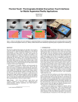
Figure 2-4 Membership Functions................................................................................... 44
Figure 2-5 Block Diagram of the Self-Validation Technique ......................................... 44
Figure 3-1 Individual Gaussian Functions and the Cumulative PDF ............................... 54
Figure 3-2 Estimation of the Measurand Value................................................................ 56
Figure 3-3 Comparison of Estimate with the Centroid.................................................... 57
Figure 3-4 Comparison of Estimate with Peak Values.................................................... 57
Figure 3-5 Measurand Estimate with High Confidence .................................................. 58
Figure 3-6 Measurand Estimate with Low Confidence ................................................... 59
Figure 3-7 Estimation of Measurand without Considering Self-Confidence .................. 60
Figure 3-8 Estimation of Measurand Considering Self-Confidence................................ 61
Figure 3-9 Block Diagram of Multiple Sensor Fusion .................................................... 61
Figure 3-10 Estimated Value from PDF without Considering Self-Confidence ............. 63
Figure 3-11 Estimated Measurand Value Using Average Method.................................. 64
Figure 3-12 Self-Confidence of the Three Sensors.......................................................... 64
Figure 3-13 Confidence of the Estimate Value Using PDF.............................................. 65
Figure 3-14 A Closeup that Shows Effect of Not Considering Self-Confidence ............ 65
Figure 3-15 Estimated Value using PDF Considering Self-Confidence ........................ 66
Figure 3-16 Close Up of Figure 3-15............................................................................... 67
Figure 3-17 Confidence of the Estimate from PDF including the Self-Confidence........ 67
Figure 3-18 Multiple Sensor Fusion without trend information....................................... 70
10
Figure 3-19 Confidence Plot............................................................................................. 71
Figure 3-20 Sources of Trend Information ....................................................................... 71
Figure 3-21 General Methodology for Sensor Fusion using Trend.................................. 74
Figure 3-22 Distributions of Trends and Fused Trend...................................................... 75
Figure 3-23 Distribution of Temperatures at the previous instant.................................... 76
Figure 3-24 Final Distribution of Temperature ................................................................ 76
Figure 3-25 Multiple Sensor Fusion Considering Trend .................................................. 77
Figure 3-26 Distributions of Trend after accounting for agreement between sensor trends
................................................................................................................................... 78
Figure 3-27 Multiple Sensor Fusion after filtering ........................................................... 79
Figure 3-27 Fused Confidence Plot ................................................................................. 80
Figure 3-27 Failure of a Sensor ........................................................................................ 82
Figure 3-27 Trends after considering Linguistic Source .................................................. 84
Figure 3-27 Sensor Fusion with Linguistic Trend Information ........................................ 84
Figure 3-27 Another Case of Sensor Failure .................................................................... 86
Figure 3-27 Multi-Modal Sensor Fusion with Linguistic Sources ................................... 86
Figure 3-27: Cupola temperature data .............................................................................. 89
Figure 3-28 Low sampling rate signal X 2 [n] ...................................................................... 90
Figure 4-1 Wrong Estimate from the Multiple Sensor Fusion ......................................... 93
Figure 4-2 Schematic Diagram of the System with Sensor Fusion Integrated with the
Controller .................................................................................................................. 95
Figure 4-3 Uncertainty in the Estimate from Multiple Sensor Fusion............................ 100
Figure 4-4 Region of Stability ....................................................................................... 101
Figure 4-5 Membership functions of the error in melt rate (eMRate) ............................ 108
Figure 4-6 Membership functions of the change in error for the melt rate (deMRate) .. 108
Figure 4-7 Implementing a Smith predictor.................................................................... 109
Figure 4-8 Simulation layout .......................................................................................... 112
11
Figure 4-9 Step response under ideal conditions ............................................................ 117
Figure 4-10 Step response with noisy outputs ................................................................ 118
Figure 4-11 Step response with input disturbances generated with square waves ......... 118
Figure 4-12 Response for melt rate confidence of 0.9 and –0.1 pulse for 600 seconds . 120
Figure 4-13 Response for melt rate confidence of 0.5 and –0.1 pulse for 600 seconds . 120
Figure 4-14 The results of varying the model parameters .............................................. 122
Figure 4-15 Smith predictor with a +600 second time delay plant offset....................... 123
Figure 4-16 Smith predictor with a -600 second plant time delay offset........................ 124
Figure 4-17 System Performance Under Effect of All Disturbances ............................. 125
Figure 5-1 Configuration for Interfacing I3PSC with ALRC DAQ for Demo Runs...... 132
Figure 5-2 Control of Carbon Content, Run #2 .............................................................. 135
Figure 5-3 Metal Stream Changes suggested by I3PSC for control of %C for Run #1 . 135
Figure 5-4 Individual Measurements and Fused Melt Rate for Run #1 ......................... 136
Figure 5-5 Confidence of Fused MR .............................................................................. 136
Figure 5-6 Individual Measurements and Fused Temperature ....................................... 137
Figure 5-7 Confidence of Fused Temperature ................................................................ 137
Figure 5-8 Oxygen Enrichment for Temperature Control for Run #1............................ 138
Figure 5-9 Blast Rate for Melt Rate Control for Run #1 ................................................ 138
Figure 5-10 Control of %C during Run #2 ..................................................................... 139
Figure 5-11 Changes in MR during Run #2.................................................................... 140
Figure 5-12 Changes in MR during Run #2.................................................................... 140
Figure 5-13 Metal Stream Changes control of %C for Run #2 ...................................... 142
Figure 5-14 Forward Change in CMR to Achieve Large Change in MR (Run #3) ....... 143
Figure 5-15 Changes in Metal Stream to compensate for Change in CMR ................... 143
Figure 5-16 Changes in Oxygen Enrichment (SCFM) during Run #3 ........................... 144
Figure 5-17 Changes in Blast Rate (SCFM) during Run #3........................................... 144
Figure 5-18 Control of Melt Rate during Run #3 ........................................................... 145
Figure 5-19 Changes in Iron Temperature deg F during Run #3.................................... 145
12
Figure 5-20 Changes in % Carbon during Run #3.......................................................... 146
Figure 5-21: Detection of Bridging in the Cupola-Changes in Exit Temperature .............................. 147
Figure 5-22: Detection of Bridging in the Cupola-Changes in Cupola Pressure ................................ 148
Figure 5-23: Opening the Tap-hole at ALRC Cupola ................................................... 149
Figure 5-24: Cupola Always Provides Operational Challenges .................................... 149
Figure 5-25: An Overview of the ALRC Research Cupola........................................... 150
Figure 5-26: Manual Sampling and Quick Analysis of Molten Iron ............................. 151
Figure 5-27: Manual Measurement of Temperature of Molten Iron ............................. 151
Figure 5-28: Optical Pyrometers for Continuous Measurements of Iron Temperature` 151
Figure 5-29: A Dip Thermocouple for Continuous Temperature Measurement ........... 152
Figure 5-30: Charging Deck of the Cupola at ALRC .................................................... 152
Figure 5-31: Measurement of Melt rate, Chemical Composition, and Temperature .... 153
Figure 5-32: Remote Monitoring and Control of the Cupola during Demo Runs......... 153
1
13
Chapter 1
1.1
Introduction
The cupola furnace is used by the iron foundry industry to melt scrap steel, cast
iron and alloying materials into a consistent grade of iron for casting purposes. There are
approximately 400 cupolas in the United States, which accounts for 70% of cast iron
production [28]. With an industry estimate of 60% yield on castings, this equates to the
direct production 1.204 million tons of carbon generating 4.412 million tons of carbon
dioxide per year. This amounts to 1-2% of the total annual national production of green
house gas [29]. The cupola has maintained its competitiveness for several reasons.
Compared with competing technologies such as arc or induction melting, the cupola uses
the energy in coal more efficiently because it does not have to go through the
intermediate step of producing electricity, and the required coke making consumes little
energy. The combustion products in cupola melting are easily contained, another
advantage over arc melting. The cupola is a relatively simple device that can be made in
many sizes to suit the molten metal needs of foundries of various sizes.
While cupola melting is simple in principle— burning coke with an air blast and
melting metal— the actual physical and chemical details of the process are quite
complex, and the phenomena occurring in the melt zone are difficult to measure directly
14
because of the aggressive chemical environment that exists inside the cupola. Controlling
these phenomena is desirable, however, for efficient energy use, for producing iron of
acceptable quality, and for reducing the environmental impact of the melting process.
The inevitable random variations in charge composition, blast effectiveness, and even
local meteorological conditions, however, lead to a degree of variability in the cupola
output. This variability can be reduced by expert operation of the cupola by experienced
personnel. Reducing this variability is more important for some cast products than for
others; where iron temperature and composition are crucial, as in the production of
automotive parts, holding furnaces, sometimes hundreds of tons in size, are used to pool
the output of one or more cupolas, and temperature and composition can be adjusted
before the hot metal goes to the casting line [28].
The economic and environmental costs of this variability can be substantial. Iron
that fails to meet specifications can cause substandard castings or even casting failure; the
material may be re-melted, but the energy spent melting it the first time is wasted. The
costs of installing, maintaining, and operating large holding furnaces to level out the
variability is an additional cost of producing iron. Materials such as coke breeze (fines
from the handling of coke) that would cause poor operation if charged from above can
also be injected through the tuyeres for added energy; the incinerator-like nature of the
cupola incorporates these, and even other hazardous wastes unrelated to cupola operation,
into the relatively benign cupola outputs: cast iron, CO, CO2, and slag.
15
1.2
Objectives and Scope of the Project
The purpose of the project was to develop and demonstrate an intelligent, integrated
industrial process sensing and control system, or I 3 PSC for short, for the foundry cupola,
the primary industrial process used for producing cast iron. However, the I 3 PSC is a generic,
enabling, cross-cutting technology that can be broadly applied to advanced process sensing and
control problems in the ferrous metal casting industries as well as in other industrial
environments. The project addressed two main objectives:
A. Development of a generic architecture for the integrated, intelligent industrial process
sensing and control system. The proposed I 3 PSC architecture is characterized by
•
Intelligent signal processing capabilities and sensor fusion methodologies,
•
Intelligent algorithms for hybrid model fusion,
•
Methodologies for integrating intelligent signal analysis and sensor and model
fusion algorithms with intelligent model-based control methodologies,
•
An object oriented generic architecture for integrating all system components.
•
Implementation of the intelligent signal processing and sensor fusion
algorithms through hardware realization using reconfigurable logic,
B. Demonstration of the application of I 3 PSC to the specific industrial setting of cupola iron
melting furnaces). The demonstration will include:
16
•
Testing of the developed algorithms using experimental data, and static and
dynamic models available from a production cupola and the ALRC research
cupola,
•
Implementation of the developed algorithms on the 18-inch research cupola at
DOE’s Albany Research Center (ALRC) ,
•
Testing the developed I 3 PSC for regulations of melt rate, temperature,
and selected iron composition on the ALRC experimental cupola furnace.
17
1.3
Deliverables
The final goal of this project was the development of a system that is capable of controlling
an industrial process effectively through the integration of information obtained through
intelligent sensor fusion and intelligent control technologies. The industry of interest in this
project was the metal casting industry as represented by cupola iron-melting furnaces.
However, the developed technology is of generic type and hence applicable to several other
industries. The system architecture was divided into the following four major interacting
components:
1.
An object oriented generic architecture to integrate the developed software and hardware
components
2.
Generic algorithms for intelligent signal analysis and sensor and model fusion
3.
Development of supervisory structure for integration of intelligent sensor fusion data into
the controller
4.
Hardware implementation of intelligent signal analysis and fusion algorithms
Table 1-1 lists the deliverables as they appeared in the proposal. They are listed here
for completeness. As will be illustrated in the current report, the objectives stated in the
proposal have been achieved.
18
Table 1-1 I3PSC Project Tasks
Task #
Description
1
Generic Structure for Integrating Sensor Fusion and Control
System Components
2
Algorithms for Intelligent Signal Preprocessing, Multi-Modal
Sensor Fusion, Model Fusion, Sensor and Model Fusion
3
Re-configurable Logic Implementation for Intelligent Signal
Processing and Sensor Fusion Algorithms
4
Algorithms for Integration of Intelligent Sensor Fusion Data into
the Controller
5
Prototype Implementation and Testing for ALRC Cupola
1.4
Project Organization, Administration, and Execution
1.4.1
Management Organization
This project represented a model for collaboration between technical developers,
industry oversight, and end users as represented in Figure 1. The technical expertise was
provided by:
1-
Tennessee Technological University ((TTU) as the main contractor,
19
2-
Utah State University (USU) as a subcontractor,
3-
Idaho National Environmental and Engineering Laboratory (INEEL) as a
subcontractor, and
4-
Albany Research Center (ALRC) as a subcontractor.
The industry oversight was provided by American Foundry Society (AFS) and the end
users represented by General Motors (GM).and US Pipe.
Detailed management organization of the project technical development team is shown in
Figure 2. The main tasks of the project are listed in Table 1 along with the groups responsible
for the completion of each task.
1.4.2
External Advisory Board
In a kickoff meeting in Detroit in January 1999, TTU, USU, INEEL, GM and
AFS agreed to create an external advisory board for the project under the direction of the
AFS. This board had representatives from foundries and industrial control companies
and will serve to assess the progress of the project and the achievement of its goals.
Collaborators arranged several meetings with the advisory board over the period of the
project. These meeting were coordinated with meetings of the AFS cupola steering
committee. The purposes of these meetings were to review the status of the completion
of the project, exchange ideas among collaborators and external advisory board and to
inform the industry about the benefits of the technology and its potential advantages.
20
1.4.3
Coordination of Teams Efforts
Coordinating the efforts among the teams working on the project was the
responsibility of the principal investigator. This coordination was achieved through
continuous communication through:
•
Use of Email and Phone, as needed, to address individual teams concerns, problems
or achievements. Emails could be addressed to a specific team leader or to the PI.
•
Conference calls were scheduled as needed, among TTU investigators and
investigators from USU and INEEL to discuss the progress and coordinate the efforts.
•
The meetings with the advisory boards were used to have technical meeting among
the technical developers at TTU, USU, INEEL, and ALRC.
•
A web site and ftp sites were developed where technical materials were exchanged
among the collaborators. (www.ece.tntech.edu/I3PSC)
21
Industry
Oversight
End User
American
Foundreymen's
Society
General Motors
Technical Development
Tennessee
Technological University
Utah State University
Idaho National Engineering
Laboratory
Albany Research
Center
Figure 1-1: Graphical Representation of Project Organization
Mohamed Abdelrahman
Principal Investigator
Mohamed Abdelrahman
PI
Jeff Frolic
Faculty Investigator
Roger Haggard
Faculty Investigator
Kevin Moore
Faculty Investigator
W. Mahmoud
Faculty Investigator
Graduate
Research
Assistant
TTU_Group1
INEEL
Graduate
Research
Assistant
TTU_Group2
Denis Clark
Investigator
Graduate
Research
Assistant
Graduate
Research
Assistant
TTU_Group3
USU
Paul King
Investigator
Technicians & Engineers
ALRC
Figure 1-2 Detailed representation of Project Organization
22
1.4.4
Overall System Vision
Figure 3 shows a schematic of the different components developed in this project
and how they are tied together for a cupola furnace application. The system is generally
divided into online and offline components. The offline analysis component is aimed at
analyzing the data collected during a heat and plan for next heats. This analysis is based
mainly on cupola models. The model currently in use is the model developed by the
American Foundry Society (AFS). However, the developed tool can be adapted to accept
other models as they become available. The online component is aimed at actual analysis
and control of the cupola furnace during a heat. It is composed of several modalities that
handle the data as it is collected from the sensors, fuse this data along with other data that
are pertinent to the cupola operation such as data coming from other sensors, virtual
sensors, models, or expert systems (MMSF). The data is then fed to an intelligent
controller, which decides based on the required operational parameters, which input
variables to manipulate. The required operational parameters are fed to the controller
using the planner. The planner can be used, by the user, to plan, offline, how the heat
will be conducted. However, it can also be used online to make changes, as appropriate,
to the heat plan.
23
Figure 1-3 Overall System Vision for I3PSC applied to Cupola Furnaces
1.5
Evaluation based on Proposed objectives:
In fulfilling the proposed objectives, the following has been achieved:
•
Innovative sensor fusion algorithms based on a new concept has been developed,
implemented and tested.
These Algorithms allow for the fusion of quasi-
redundant sensors data and produces a best estimate and a parameter indicating
the degree of confidence in the measurement. The algorithms were presented in
conference publication namely, the American Control Conference (ACC), and
24
published in the prestigious journal of IEEE Transactions on Instrumentation and
Measurements.
•
The developed algorithms were improved to incorporate trend information as well
as linguistic information. This allows for the fusion of information from sources
other than physical sensors such as virtual sensors, models and expert system
information.
•
Generic algorithms for the integration of sensing and control based on the
previously developed algorithms for sensor fusion were developed and
implemented.
•
The developed generic algorithms for sensor fusion and integration of sensing and
control represent advances in basic science. The researchers have also presented
application specifically for cupola furnaces. These results were presented at
professional conferences with audience interested in the advancement of melting
methods.
•
Algorithms for the implementation of the sensor validation and multiple sensor
fusion algorithms on hardware were developed, simulated and tested .
•
A generic data structure and an object oriented based software package were
developed for the incorporation of the different algorithms. The current package
incorporates the following modules:
o A Data Acquisition modality for interfacing with existing data acquisition
system in a cupola or other industrial plant,
25
o A planner modality where a plan for the cupola heat can be developed,
o
A sensor fusion modality,
o A virtual sensors modality for predicting values of some important
parameters based on other system measurements,
o A controller modality for producing suggested values for the manipulated
variables based on the system requirements,
o A monitoring modality for monitoring trends of specific variables and
alerting operator when certain patterns take place.
The software and data structure were designed to allow for easily
incorporating other modalities and modifying the existing ones.
•
The integrated system was successfully demonstrated on a research cupola facility
in Albany Research Center, Albany, Oregon. The demo involved successful
interface of the developed system to the existing DAQ system, monitoring and
controlling the main parameters of the cupola furnace, namely, molten iron
temperature, melt rate and Carbon composition using manipulated variables,
namely, oxygen enrichment, blast rate, steel/cast ration and coke/metal ratio. The
control system ability to achieve and maintain operational parameters as well as
reject disturbances and minimize transition periods was illustrated.
A list of the papers supported by the project and published in refereed journals
and conferences is presented in Appendix 1.A. A list of academic theses supported by
26
the project is listed in Appendix 1.B.
Other information pertaining to the project
achievements were presented in previous reports [32] - [34].
1.6
Summary and Report Organization
In summary, the project has achieved all the proposed objectives starting from
development of algorithms for sensor validation and fusion, integration of sensing and
control, development of a package for integrating system components and a proof of
concept of using FPGA to implement sensor fusion algorithms.
The project has
supported the development of basic science in the form of publications in professional
refereed journals and conferences as well as practical and applied science with reference
to cupola furnace as evidenced by demonstration using cupola furnace data and models
and actual demo plans on a research cupola.
This report is divided into two sections. Section 1 describes a subset of the developed
algorithms and results of demonstration runs.
Chapter 1 summarizes the project
organization, objectives and results of the project. Chapters 3 and 4 provide a description
of the basic algorithms that were developed for sensor fusion and control.
More
information can be found in the published work listed in Appendices 1.A and 1.B. A brief
description of the developed software package is provided in the form of a user manual in
Appendix A of Section One. Section 2 describes the hardware implementation. Chapters
1-3 describe work accomplished during project years. Chapter 4 gives a summary of the
27
work accomplished and future recommendations. The section ends with Appendices that
describes more details of the algorithms hardware implementation.
28
Appendix 1.A
List of Publications Supported by the Project
1. Jeff Frolik, Mohamed Abdelrahman, and Param Kandasamy, “A confidence
Based Approach to the self-validation, fusion and reconstruction of quasiredundant sensors," IEEE Transaction on Instrumentation and Measurement. ,
Vol. 50, No. 6, December 2001.
2. Mohamed Abdelrahman and Param Kandasamy, “Integration of Multiple Sensor
Fusion In Controller Design,” Accepted for Publication in the Transactions of
Instrumentation Society of America, 2002.
3. Mike Baswell and Mohamed Abdelrahman, “Fuzzy Control Of A Cupola Iron
Melting Furnace,” To Appear in Transactions of American Foundry Society,
2003.
4. Mohamed Abdelrahman and Param Kandasamy, “Integration Of Intelligent
Industrial Process Sensing and Control for Cupola Iron Melting Furnace,” in
proceedings of the 7th Mechatronic Forum International Conference, Atlanta, 6 –
8 September, Atlanta, GA, 2000.
29
5. Mike Baswell and Mohamed Abdelrahman, “Fuzzy Control Of A Cupola Iron
Melting Furnace,” AFS Congress, Kansas City, MO, May 2002.
6. Min Luo and Mohamed Abdelrahman, ”Wavelet-Based Sensor Fusion for Data
with Different Sampling Rates,” ," in Proceedings of American Control
Conference, Washington D.C., June 2001.
7. Mohamed Abdelrahman et al, "A Methodology For Fusion Of Redundant
Sensors," in Proceedings of American Control Conference, Chicago, IL, June
2000.
8. Jeff Frolik and Mohamed Abdelrahman, "Synthesis of quasi-redundant sensor
data: a probabilistic approach," ," in Proceedings of American Control
Conference, Chicago, IL, June 2000.
9. Steve Orth, Jeff Frolik and Mohamed Abdelrahman, "Fuzzy rules for automated
sensor self-validation and confidence measure," in Proceedings of American
Control Conference, Chicago, IL, June 2000.
10. Vipin Vijayakumar and Mohamed Abdelrahman, "A convenient methodology for
the hardware implementation of fusion of quasi-redundant sensors," Proceedings
of 32nd SSST Conference, Tallahassee, FL, Mar 2000, pp. 349-353.
11. Param Kandasamy and Mohamed Abdelrahman, "A Methodology for Integrating
nd
Multiple Sensor Fusion in the Controller Design," in Proceedings Of 32
conference, Tallahassee, FL, March 2000, pp. 115 -118.
SSST
30
12. Mike Baswell and Mohamed Abdelrahman, “Intelligent Control of Cupola
Furnaces,” in Proceedings of the 34th SSST conference, Huntsville, AL, March
2002, pp. 435-440.
13. Wagdy Mahmoud, “Hardware Implementation of Automated Sensor Selfvalidation
System
For
Cupola
Furnaces”,
in
Proceedings
of
31st
conference on Computers and Industrial Engineering, San
Francisco, CA, Feb 2-4, 2003.
14. Mohamed Abdelrahman et al, “A Methodology For Multi-Modal Sensor Fusion
Incorporating Trend Information”, in Proceedings of 31st conference on
Computers and Industrial Engineering, San Francisco, CA, Feb 24, 2003.
31
Appendix 1.B
Theses supported by the project
1. Min Luo, Fusion of Multi-resolution Sensors using Wavelet Transform, Tennessee
Technological university, September 2001.
2. Vipin Vijayakumar. A Methodology for Multi-Modal Sensor Fusion. June 2001
3. Parameshwaran Kandasamy. Development of Sensor Fusion Algorithms for
Redundant
Sensors
and
Integration
in
Controller
Design,
Tennessee
Technological university, May 2000.
4. Avinash Seegehalli. Multi Dimensional Data Structure for Cupola Furnace
Information Processing, USU, 2000.
5. Jie Chen. Detection and Extraction of Parallel Hardware During C to VHDL
Translation, Tennessee Technological University, May 2003.
6. Sobha Sankaran. Hardware/Software Codesign - Efficient Algorithms for
Hardware Synthesis from C to VHDL, Tennessee Technological University, 2001.
7. Srikala Vadlamani. Comparison of Cordic Algorithms Implementation on FPGA
Families, Tennessee Technological University, 2002
32
33
Chapter 2
2
MOTIVATION and OVERVIEW
Feedback control systems have gained extreme importance in modern engineering
world.
Feeding back the output has made it possible for systems to perform their
assigned tasks with better reliability.
A number of control techniques have been
developed to achieve the desired response from a feedback control system.
These
techniques achieve accurate tracking of the system output along a specified reference
value [1]. There are also robust techniques that can achieve good performance even if the
system is not modeled accurately [2]. Robust feedback control system also reduces the
sensitivity of the system with respect to the system parameter variation and external
disturbances. A schematic diagram of a general feedback control system is shown in
Figure 2-1.
Reference
Input
Error
Detector
Output
Controller
Plant
Feedback
Element
Figure 2-1 Schematic Diagram of a Feedback Control System
34
2.1
Motivation
Sensors are used to measure and feedback output data in feedback control systems.
The feedback data are used to decide the necessary control action. The performance of a
feedback control system depends heavily on the reliability of the sensors' readings. There
are different reasons why the sensor data may not be reliable. These reasons include:
1) Sensors may be prone to high levels of noise and disturbances during measurement
and transmission of the data;
2) Sensors' characteristics may vary with changes in environmental parameters, such as
the temperature, humidity, or due to aging;
3) Accurate measurement of some variables may not be possible due to the physical
nature of the process; and
4) Failure of electronic circuitry of the sensor.
There are several methods available to increase the reliability of process
measurements using redundant sensors. The redundancy may be achieved through
physical sensors, analytical sensors, or inferential sensors. Analytical sensors depend on
a model of the physical process to estimate the value of the intended system parameter.
Inferential sensors utilize other output variables to infer estimates for different variables.
Techniques such as signal validation and multiple sensor fusion are usually used to get a
better estimate for the desired variable. These techniques will be discussed in detail in
35
Chapter 2. A schematic diagram of a closed loop system that utilizes the multiple sensor
fusion is presented in Figure 2-2.
Analytical Sensors
Best Estimate
Reference
Input
Error
Detector
Multiple
Sensor
Fusion
Controller
Inferential Sensors
Redundant
Physical
Sensors
Plant
Inferential
Sensor
Plant
Model
Analytical
Sensor
Figure 2-2 A Feedback Control System with Multiple Sensor Fusion
The above techniques are used to reduce the sensitivity of the system performance
with respect to sensors' failures. This is accomplished by not relying on a single sensor
measurement.
For multiple sensor fusion or signal validation techniques to work
satisfactorily, certain conditions need to be satisfied. These include, for example, the
availability of redundant sensors, an accurate plant model, or known relations between
variables. Since most techniques still rely back on other sensors for the feedback value,
there will be situations where the feedback value is not reliable. A measure for the
performance of the signal validation or multiple sensor fusion technique needs to be
developed and utilized in the controller structure.
36
2.2
Research Approach
The research focus of this report is to develop a methodology to prevent the
performance degradation of an automatic control system due to unreliable sensor data.
The suggested solution to the problem is twofold:
1) The development of a multiple sensor fusion algorithm that can produce a best
estimate and reliability measure for the estimate of the sensor data.
2) The development of a controller structure, which utilizes the estimate and the
reliability measure to change its performance, so as to prevent costly mistakes.
The methodology developed should reduce the sensitivity of the system to the
sensor data when the reliability of the sensor data is found to be low. This is achieved by
changing the controller's dependability on the sensor signal according to the reliability
measure from the multiple sensor fusion.
A block diagram of the feedback control
system to be developed is shown in Figure 2-3. It resembles Figure 2-2, but for the
additional flow of information, the confidence, from the multiple sensor fusion block to
the controller.
37
Analytical Sensors
Best Estimate
Multiple
Sensor
Fusion
Inferential Sensors
Redundant
Physical
Sensors
Confidence
Reference
Input
Error
Detector
Controller
Plant
Inferential
Sensor
Plant
Model
Analytical
Sensor
Figure 2-3 Block Diagram of Proposed System
The problem considered in this report is that the performance of the
feedback controller degrades when the feedback signal from the sensor data is unreliable.
The problem of increasing the reliability of the feedback signal was tackled in many
ways. The most common method used to increase the reliability of the feedback signal is
multiple sensor fusion. One other approach is to check the reliability of each sensor by
using self-validation. In this chapter, a quick review of some of these multiple sensor
fusion and self-validation techniques is presented.
A basic overview of adaptive
controllers and some adaptive methods are also discussed.
2.3
Multiple Sensor Fusion and Signal Validation
2.3.1 Multiple Sensor Fusion
Sensor fusion is defined as the method to fuse or manipulate information from
different sensors and come up with one value of interest. These sensors may measure the
38
desired measurand or may measure different values, which should be combined to get the
required information. If the different sensors are measuring the same quantity, then these
sensors are called redundant sensors. In this report multiple sensor fusion is constrained
to mean only the fusion of redundant sensors.
There are many reasons why multiple sensor fusion is used. Combining several
sensors' data will give more accurate information of a measurand improving the
reliability of measurement data. The measurement data become less sensitive to noise
and disturbances that might not affect all the sensors, when many sensors are used.
Efficiency and performance of the measured data are enhanced [3].
Several techniques are available to fuse the values from the redundant sensors [4].
The most obvious approach is to find the average of the sensor data. In this case,
however, the estimate will be affected by the invalid sensor data. A simple improvement
to this was to have a weighted average of the redundant information. A weight is given
to each sensor depending upon a threshold. The threshold for the current decision is
usually the previous estimate. This helps in eliminating the spurious data. The choice of
threshold is important in this method. If the process data has large variations between
adjacent values, the threshold technique may result in removing valid sensor data.
Kalman filtering technique is generally used for sensor fusion where Gaussian
noise exists. The performance of the Kalman filter technique depends upon the accuracy
of the system model [Chapter 12, [3]]. It gives better results if there exists a linear model
to the system and if both the system and the sensor noise can be modeled as Gaussian
39
noise. Finding an accurate model for systems is not always possible in many cases and
most of the real time systems are nonlinear.
A method developed by Luo and Lin [5] finds the estimate from the multiple
sensor fusion of only consensus sensors. The method first eliminates those sensors' data
that are likely to be erroneous. This is accomplished by using a probability density
function(PDF) around each sensor's data. This PDF around each sensor's data is used to
find the distance from other sensors' data. This distance measure is stored as a matrix for
each sensor, which are combined later to find a combined matrix from which the optimal
fusion estimate is found. This method of having an individual matrix and forming a
combined large matrix that is reduced to get optimal value is called the Bayesian
approach [5].
Many others also approach the multiple sensor fusion problem by finding the best
combination of sensors that are to be fused. The search is based on the distance between
the sensors, each sensor's failure rate and its previous data. Algorithms like neural based
search and genetic algorithms were used [Chapter 10, [3]]. The combination of selected
sensors is then usually averaged to find the estimate.
The performance of these
approaches depends on the search algorithm. These are best suited for decision-making
sensor fusion problems.
As an extension to the above search first and then fuse, multiple sensor fusion is
implemented using approximate agreement approach in [Chapter 11, [3]].
The approach
first establishes an agreement set on each sensor data. This is done by each sensor
40
broadcasting its value to other sensors. Each sensor then forms the agreement set based
on the distance from other sensor data. This agreement set helps in eliminating invalid
sensor data and find the estimate on which most sensors agree. This approach requires
3t+1 sensors with t+1 giving accurate reading, where t is the number of faulty sensors.
The mean of the agreement set after removing t lower and t higher data gives the
estimate. This algorithm is again best suited for binary decision-making (Target or no
Target).
Multiple sensor fusion techniques use the redundant data and come up with one
value. Each sensor data have an effect on the final estimate. A failed sensor will have
adverse effect on the estimate if not removed. So it is necessary to validate the sensor
data before fusing the redundant data and remove the sensor. The next section discusses
some of the signal validation techniques that achieve this.
2.3.2
Signal Validation
Signal validation is a technique by which the sensor's signal is validated for its
accuracy. Signal validation may involve all or one of the following: detection, isolation,
and characterization of faulty sensors [6]. Most of the initial researches depended on
finding an additional measure for the sensor, either by having redundant sensors or by
producing an analytical redundancy to the sensor data by using a model for the process.
A detailed survey of the signal validation using redundant sensors based on
statistical methods is described in Ray and Luck [7]. The statistical approach is based on
the difference between the current sensor data and other redundant sensor data. Fuzzy
41
logic (FL) is also used for signal validation using redundant sensors. The advantage of
using FL is that the strict boundary posed by the numerical sensor data can be replaced
with linguistic terms [6].
Analytical redundancy is used in situations where physical redundancy is not
possible.
Analytical redundancy is created using a model for the process. Neural
networks have been used to create the analytical redundancy using historical data of the
process [8]. Combinations of fuzzy and neural systems have been used to create
analytical redundancy for a specific sensor. Another type of redundancy is created using
inferential sensors. The redundancy is obtained from using sensors that measure other
variables and the relationship between the variables and the variable of intent. Genetic
algorithm is used to find empirically the variables best suited for use in the inferential
redundancy while neural based fuzzy system is trained to estimate the monitored sensor
signal [9].
These analytical and inferential redundancy are then treated as physical
redundancy and used in validating physical sensor data.
There are many difficulties in creating physical or analytical redundancy for
sensor signals like increased cost, complexity in hardware implementation for the
sensors, and uncertainty in modeling the plant. Moreover, the reliability of the sensors
that are used for the redundant measurement cannot be assumed. Hence, few researchers'
started to work on the validation of sensors using data from the sensor that is being
validated. This is discussed in the next section.
42
2.3.3
Self-Validation
The technique of validating a sensor using the historical data from that sensor
alone is called self-validation. These self-validating sensors are called intelligent sensors
and many researches are taking place to create intelligent measurements. Yang and
Clarke in their section [10] have defined the self-validating sensors, their rationale, and
how they can evolve into intelligent measurements.
Initial research in this area started by considering the invalid data of sensors as
noise and hence using filtering techniques for the self-validation. Kalman filter was found
to give good results for self-validation. A detailed description of self-validating sensors
was given in Henry and Clarke [11]. The research by Tsai and Chou [12] uses the
correlation of system dynamics with multistep readings of a sensor.
Using historical data of the sensors for self-validation was used by Mercadal [13].
This reference paper uses the historical data to create an analytical model for the sensor
depending upon its previous values.
The actual sensor data are then validated by
comparing it with the value predicted from the model.
The paper [14] develops a fuzzy based self-validating algorithm based on the
validated historical data of the sensor. The algorithm developed in this paper is described
in detail as it is implemented and used as a part in this report. In this paper a measure of
reliability of the sensor data, called self-confidence, is obtained. Self-confidence is a
measure of the agreement between the characteristics of current sensor data and historical
43
sensor data that are deemed valid. This self-confidence can be used for the detection and
isolation of faulty sensors.
An FL-based system is developed based on same basic rules that characterize the
sensor data, namely:
1) The data from the sensor should be within a valid range;
2) The absolute value of the rate at which data varies should not be higher than a given
threshold that is determined using historical data;
3) The standard deviation of the sensor data within a certain window should be less than
a given threshold; and
4) The standard deviation of the sensor data should not be zero, which would indicate a
constant value. This indicates that the sensor is not working properly.
These requirements are coded as rules in the fuzzy system. The input variables
used are the data, rate of change in the data, and the standard deviation of a certain
window. The membership functions for these input variables are defined by finding the
variation and the trend in the historical data. The membership functions are shown in
Figure 2-4. The limits in the membership function, namely MT1, MT2, etc., are found
from the processing of the historical data. The deviation of the data from the curve is
considered as the standard deviation of the sensor.
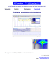
The block diagram of the self-
validation algorithm from the paper is shown in Figure 2-5.
44
MemberShip Function1 - Temperature
Ideal
Low
MT1
MT2
MT3
High
MT4
Membership Function2 - Rate of Change in Temperature
Very_Negative
Small
-MR8
-10*MR8
-MR7
Very_Positive
MR7
MR8
10*MR8
Membership Function 3 - standard Deviation
Constant
Normal
MS1/2 MS1
High_Noise
MS2
MS3
10*MS3
Figure 2-4 Membership Functions
Acquire Data
Set
Acquire Real
Data
(Runtime)
Pre-process
Data
Median Filter
Create
Parameters from
Verified Data
Set
Pre-Processing to
calculate input
parameters
Create Fuzzy
Membership
Functions from
Parameters
Fuzzy System
Figure 2-5 Block Diagram of the Self-Validation Technique
Obtain
Confidence
45
The rules of the fuzzy system remains the same for all sensors while the
membership function varies from one sensor to another sensor depending upon the
sensor's historical data. The fuzzy output gives the self-confidence of the sensor. The
median output of the data is the sensor data output of the self-validation.
2.4
Adaptive controllers
Controllers are designed based on the model of the plant.
Earlier control
designers assumed exact knowledge of the plant and that the plant is modeled accurately.
These controllers demanded accurate measurement of the state variables that are used for
controlling the performance of the plant.
It was soon realized that meeting these
requirements is not possible in all situations and people tried to design controllers that are
robust. Many robust control design techniques were developed and these controllers
were able to tolerate the variation in the model, system parameters, and state variable
estimations. But, these controllers achieved them at the cost of performance [15].
Adaptive controllers provide an answer to the problem. Adaptive controllers are
basically a controller whose control law adapts its own behavior as it learns about the
process it is designed to control or as the process changes with its environment. The field
of adaptive control is a very wide and what is presented in this section is a brief
introduction to adaptive control. It is not intended to be a thorough literature review.
Adaptive control methods are classified into two broad categories [15]:
46
1) Indirect or explicit control. - The basic requirement in this method is the availability
of a design model, but the parameters of the model are not known. The plant
parameters are estimated explicitly on-line and the control parameters are then
adjusted based on these estimations.
Indirect control methods utilize separate
parameter identification and control schemes.
2) Direct or implicit control. - This method does not assume the availability of the
design model. The controller parameters are adjusted directly, only using plant input
and output signals. The identification and control functions are merged into one
scheme.
Many adaptive control approaches have been developed. Gain scheduling, selftuning of the controller, model reference adaptive control, and variable structure adaptive
control are some of the most commonly used approaches. All of these approaches fall in
one of the two categories mentioned above [16]. Few approaches that involve both the
direct and indirect method have also been developed.
Gain scheduling is the simplest type of the adaptive control. In this approach, the
controller gains are made dependent on the parameters that can be measured or inferred
from other measurements. This approach is very conservative and poses many problems
if the dependent parameter has high rate of variation [15].
Parameter estimation forms the base for self-tuning. The required parameter is
modeled and an observer is implemented to estimate the parameter. The controller is
designed as a dependent on the estimated parameter. This method requires all the state
47
variables for parameter estimation, which is not possible in all systems [16]. Using state
estimator may help, but it results in a complex system.
Model reference adaptive control is based on a reference model for the plant. The
error between the actual output and the output from the reference model is used to change
the controller parameters.
This approach introduces a lot of nonlinearity through
multipliers and additional error processing.
Hence, determining the stability of the
system is very difficult [16].
Variable structure adaptive control from input and output variables has been
discussed in the paper [17]. Variable structure is similar to model reference adaptive
control but instead of using parameter estimation, it uses signal synreport.
A
discontinuous switching control function is designed to generate the sliding surface for
the variable structure adaptive control. The paper derives the stability of the adaptive
control.
The disadvantage of the variable structure control is that it requires the
knowledge of all state variables. State estimator may be used, but it results in a complex
system.
In [18] Burdet and Codourey compares most of these adaptive control algorithms
and have tested experimentally two of the best algorithms. It was shown that the
Adaptive FeedForward Controller (AFFC) is well suited for learning the parameters of
the dynamic equation. The resulting control performance is compared with the measured
parameters for any trajectory in the workspace and was said to give better results. The
48
paper also introduces an adaptive look-up-table memory and was shown to be simpler
and better for tasks that requires repeating the same trajectory.
In [19], another type of adaptive control based on switching the controllers is
developed. In this paper the output of the plant with unknown parameters were made to
track the reference signal through switched nonlinear feedback control strategy. Many
controllers were designed and the controllers are selected online through a performance
evaluation procedure that uses the output prediction error. The paper also discusses
sufficient conditions under which the closed loop control system is exponentially stable.
This approach achieved asymptotically stable control and the results of this approach
were illustrated with three examples.
Automatic synthesizing of controllers other than gain scheduling was used in [20].
The paper describes a method that automatically derives controllers. The controllers
were derived for timed discrete-event systems with non-terminating behavior modeled by
timed transition graphs. The specifications of control requirements were expressed by
metric temporal logic (MTL) formulas. The syntheses of the controllers were performed
by using, a forward-chaining search and a control-directed backtracking. The synreport
process does not require explicit storage of an entire transition structure. This feature of
automatic synthesizing of the controllers for the above procedure of switching controllers
may compliment each other for obtaining superior performance from an adaptive
controller.
49
Adaptive controllers give better performance even when the system parameters or
the environment changes. Adaptive controllers have gained importance with rigorous
proofs for stability. Their tolerance to large parameter variations has made them more
suitable for many industrial applications.
2.5
Conclusions
Most of the literatures in multiple sensor fusion exist for detection purposes and
are developed for target or enemy detection in military-based research. Few literatures
are available on fusing redundant sensors for non-military applications. These are
commonly based on averaging the redundant data. Kalman and Bayesian methods are
based on probability density function (PDF). Kalman filtering technique, however, needs
a good model of the system, which is not always available. The Bayesian method
considers two data points at a time for a confidence measure and also involves lot of
matrix manipulations. The approximate agreement approach explains the advantages of
finding agreement between the sensors. One other factor that is required is the degree of
agreement between the sensors on the estimate value. There was no literature discussing
an algorithm to find such a measure.
Adaptive control methods are available to improve performance. The controller
parameters are adapted based on the system parameter variation, environment changes
and even with performance. However, not much of research exists in the area of adapting
the controllers based upon the sensor reliability.
50
This chapter discussed some of the self-validation techniques, multiple sensor
fusion algorithms and adaptive control approaches. The problem of improving the
performance of the system even under the failure of sensors is solved using adaptive
control approach. The self-validation technique and multiple sensor fusion algorithm is
used to decide upon the adaptation of the controller. The self-validation technique
developed in Year 1 of the project was reviewed in section 2.4. In Chapter 3, the
developed methodology for redundant as well as multi-modal sensor fusion is presented.
51
52
Chapter 3
3
MULTIPLE SENSOR FUSION
In Chapter 2, several multiple sensor fusion algorithms were discussed. Sensor
fusion is used to reduce the effect of a sensor failure over the operation of the system
considered. The signals from sensors are fused to get a better estimate of the measurand
value. Thus, sensor fusion helps in improving the reliability of the measurements that
primarily affects the performance of a system. This is especially true in the case of
feedback control systems.
Among the multiple sensor fusion algorithms discussed in Chapter 2, many
techniques build on averaging the redundant sensors' readings. However, averaging the
sensors' data would still mean that a failed sensor would affect the estimate value. So,
the factor that should be considered in the sensor fusion is the confidence in the data
obtained from each sensor. This is the concept that was introduced in section 2.2 as the
self-confidence. A multiple sensor fusion algorithm incorporating this self-confidence
will be less affected by a sensor failure.
Some of the algorithms that were studied in Chapter 2, produces an estimate that
represents the value that most sensors agree. But, these techniques do not specify the
degree of agreement on the estimate by the sensors. Hence, a multiple sensor fusion
algorithm that reflects the degree of agreement among sensors will be more appropriate.
53
In this chapter, a multiple sensor fusion algorithm that produces a measure of the
confidence in the estimated value of the measurand is developed.
The confidence
measure reflects the degree of agreement among the sensors.
First, the discussion on redundant sensor fusion algorithm and how a measure of
confidence in the estimate is produced, are presented. Next, the integration of the selfconfidence into the multiple sensor fusion algorithms to mitigate the effect of sensor
failure are presented. The multiple sensor fusion algorithm is tested using data from an
experimental run of a cupola furnace. A comparison of the results with that of the
averaging method is also discussed. A unified framework for multi-modal sensor fusion
is also presented in this chapter of the report.
3.1
Parzen-like Methodology for Redundant Sensor Fusion
3.1.1
Description of Parzen Estimator
The Parzen estimator is a nonparametric method for estimating probability density
functions without making any assumptions about the nature of the distribution [21].
Given a set of sensor data, the Parzen estimator utilizes parametric functions such as
Gaussian functions that are centered at each of the sensors’ readings. The functions are
then added up and normalized. The resulting Probability Density Function (PDF) reflects
the distribution of the sensors’ data. The PDF energy is more concentrated where more
data points exist. This is illustrated in Figure 3-1.
54
0.2
0.15
Sensor Value
Cumulative PDF
Individual Gaussian Fn.
0.1
0.05
0
0
5
10
15
20
25
Figure 3-1 Individual Gaussian Functions and the Cumulative PDF
For this research a Gaussian function (GF) is selected as the parametric function.
The mean value of the GF is equal to the sensor reading and the standard deviation is
estimated from the noise level in the sensor [14]. The PDF is given by
PDF ( x) =
1
N
N
∑
k =1
1
2π σ k
exp(−
( x − xk ) 2
2σ k
2
)
…(3.1)
where N is the number of sensors, xk is the kth sensor data, and σκ is the standard
deviation. The parameter σκ is estimated based on the standard deviation of the noise
associated with each of the sensors considered.
3.1.2 Estimation of Measurand Value from PDF
The estimate value of the measurand is calculated from the PDF obtained as
explained in previous section.
There are several ways to get an estimate of the
55
measurand value similar to defuzzification methods such as average, centroid, maximum,
and sum of the maximum [22].
In this research an algorithm was developed for
estimating the measurand value. The algorithm is an integration of the peak and centroid
methods.
1. Find the range X which contains 95% of the PDF energy.
2. Find the centroid of the PDF using:
Centroid
=
∫ x . PDFdx .
∫ PDFdx
X
X
3. Find the area on each side of the centroid.
4. The estimate is found as the value of measurand that corresponds to the supremum of
the PDF on that side of the centroid that has the higher area, thus
5. Measurand Estimate = arg(Sup(PDF))).
…(3.2)
The function arg corresponds to finding the x co-ordinate at which the maximum
value occurs in the PDF. This procedure is illustrated in Error! Reference source not
found..
56
0.2
Centroid
0.15
0.1
Estimate
0.05
0
0
5
10
15
20
25
Figure 3-2 Estimation of the Measurand Value
This particular method of finding the estimate is found to be more advantageous
than other methods as explained in this section. The estimate of the multiple sensor
fusion algorithm should be the value on which most of sensors agree, and at the same
time the estimate should not be adversely affected by invalid sensors. Other methods for
estimating the measured value from the PDF such as centroid and peak allow faulty
sensors to have an effect on the estimate or may not give the most probable value on
which the sensors agree. Figure 3-3 shows how the estimate, if chosen, using the
centroid would be affected by the faulty sensor. Figure 3-4 shows that the peak value
does not always correspond to the value on which most sensors agree, at all cases.
57
0.4
0.3
Good
Sensors
Developed
Algorithm
Centroid
0.2
Faulty
Sensor
0.1
0
6
8
10
12
14
16
18
20
22
Figure 3-3 Comparison of Estimate with the Centroid
0.4
0.3
0.2
0
Developed
Algorithm
Peak
0.1
4
6
8
10
12
14
16
18
20
22
Figure 3-4 Comparison of Estimate with Peak Values
3.1.3
Confidence in Estimate
The estimate value from the previous procedure takes into account the agreement
between the sensor data. However, the estimated value does not explicitly reflect the
58
degree of agreement between the sensors and hence the confidence in the estimated
value. The agreement between the sensors is reflected in the width of the PDF function
estimated according to the process previously described.
Thus, the confidence is
calculated using the area of the PDF that is enclosed within three standard deviations on
each side of the estimated measurand value. In the ideal case, where all the sensors agree
exactly, this will be approximately equal to one. As the agreement between the sensors'
decrease, this area will decrease as well. This is illustrated in Figure 3-5 and Figure 3-6.
The confidence is related to the PDF function width according to the relation:
Estimate + 3σ
Confidence =
∫ PDF ( x)dx
…(3.3)
Estimate −3σ
where σ is the maximum standard deviation of the parametric functions used in
forming the PDF.
0.4
Integration Limits
0.3
PDF
0.2
0.1
0
7
8
9
10
11
12
13
14
15
Figure 3-5 Measurand Estimate with High Confidence
16
17
59
0.4
Integration Limits
0.3
0.2
PDF
0.1
0
6
8
10
12
14
16
18
20
Figure 3-6 Measurand Estimate with Low Confidence
3.2
Considering Self-Confidence in Redundant Sensor Fusion
The self-confidence of a sensor data obtained from the self-validation technique
explained in section 2.2 is a measure of how much this data agrees with the expected
characteristics of the sensor as estimated from historical data. Thus, a change in the
sensor noise level or if the sensor data or its rate of change exceeds the expected limits,
the self-confidence value decreases. Integration of this self-confidence into the redundant
sensor fusion is necessary to decrease the effect of the failed sensors on the estimated
value.
In Section 3.1 the Parzen like procedure for estimating the PDF which was then
used to get a best estimate for the measurand value was presented. The function used in
Parzen estimation was a Gaussian function with a standard deviation that depends upon
the sensor noise. This Gaussian function can be thought of as a representation of the
60
probability in finding the true value of the measurand data around the sensor reading. As
the self-confidence decreases, the probability of finding the true value of the measurand
in the neighborhood of the sensor measurement decreases. In other words, the region in
which the true value could be with respect to the sensor reading becomes wider. This
could be reflected by scaling up the standard deviation of the Gaussian function, used in
building the PDF, using the self-confidences of the sensors. Thus, the PDF function
becomes
1
PDF ( x) =
N
N
∑
k =1
( x − xk ) 2
)
exp(−
2(σ k / SC ) 2
2π (σ k / SC )
1
…(3.4)
where SC is the self-confidence of the sensor and the rest of the parameters are
defined as in (3.1). Figure 3-7 and Figure 3-8 illustrate the effect of the change in selfconfidence over the shape of the Gaussian functions and hence the PDF. It should be
noted that this change is not used in the standard deviation used for finding the
Confidence.
0.4
0.3
Self Confidence = 1
0.2
PDF
0.1
0
6
8
10
12
14
16
18
20
22
Figure 3-7 Estimation of Measurand without Considering Self-Confidence
61
0.4
0.3
Self Confidence = 0.5
0.2
PDF
0.1
0
2
4
6
8
10
12
14
16
18
20
22
Figure 3-8 Estimation of Measurand Considering Self-Confidence
Median Sensor
Data
Self Center
GF
Validation
Std. Dev
R
e
d
u
n
d
a
n
t
Estimate
D
a
t
a
Self-Confidence
Self Validation
Center
GF
Std. Dev
Overall PDF
(Cumulative Confidence
and
Normalized)
Median Sensor
Data
Center
GF
Self Std. Dev
Validation
Self-Confidence
Figure 3-9 Block Diagram of Multiple Sensor Fusion
62
A block Diagram of the Multiple Sensor Fusion Algorithm Developed including
the integration of self-confidence is shown in Figure 3-9.
3.3
Application and Testing
In the following section the testing results are presented for the redundant sensor
fusion methodologies presented in sections 3.1 and 3.2. The testing was performed using
data from an experimental cupola iron-melting furnace in Albany, Oregon. The system
uses three temperature sensors that measure the temperature of the iron melt produced
from the furnace. These sensors were quasi-redundant as explained in [23]. The sensors'
data of two of the temperature sensors were translated using a linear regression relation to
give an estimate of the third sensor. The resulting data were then treated as if the sensors
were redundant sensors.
3.3.1
Results of the Sensor Fusion Methodology without Considering SelfConfidence
The results of testing the methodology of integrating redundant sensors presented
in Section 3.1 are presented first. Figure 3-10 shows the results of the test. The data from
one of the sensors (TC5) were artificially perturbed by injecting sudden disturbance at t =
10 minutes and high noise level into the sensor in the range t=40 to 70 minutes. For
comparison purposes, an estimate of the measurand value using the average of the sensor
data is presented in Figure 3-11. The self-confidences of the three sensors are presented
in Figure 3-12. Figure 3-13 shows the total confidence in the estimate. It is clear from
63
Figure 3-11 that the average method results in the estimated value to be affected by the
sudden disturbances as well as by the noise introduced into one of the sensors. In
comparison Figure 3-10 shows that the effect of the disturbances were mitigated to some
extent. However, a close up of the data in Figure 3-10 shows that the estimated value of
the measurand is still affected by the readings of the sensor, which was artificially
injected with the high noise level. This close up is shown in Figure 3-14. It should be
noted, however, that the confidence in the estimates are lower in periods where the
agreement between the considered sensors decreases as shown in Figure 3-13.
800
TC3
TC4
TC5
Estimate
750
700
650
0
10
20
30
40
50
60
70
80
90
100
Figure 3-10 Estimated Value from PDF without Considering Self-Confidence
64
800
TC3
TC4
TC5
Estimate
750
700
650
0
10
20
30
40
50
60
70
80
90
100
Figure 3-11 Estimated Measurand Value Using Average Method
1
ConfTC3
ConfTC4
ConfTC5
0.8
0.6
0.4
0.2
0
10
20
30
40
50
60
70
80
Figure 3-12 Self-Confidence of the Three Sensors
90
100
65
1
0.8
0.6
0.4
0.2
0
10
20
30
40
50
60
70
80
90
100
Figure 3-13 Confidence of the Estimate Value Using PDF
TC3
TC4
TC5
Estimate
790
780
770
760
750
50
52
54
56
58
60
62
64
Figure 3-14 A Closeup that Shows Effect of Not Considering Self-Confidence
3.3.2
Results of the Sensor Fusion Methodology Considering Self-Confidence
The test is repeated using the same data presented in Section 3.3.1. However, this
time the methodology presented in Section 3.2 is used. The self-confidences of the
sensors over the considered time period is shown in Figure 3-12. The estimates of the
66
measurand value are shown in Figure 3-15. A close up of Figure 3-15 is shown in Figure
3-16. A Comparison between Figure 3-14 and Figure 3-16 shows the advantages of
including the self-confidence in the sensor fusion methodology. When the high noise
level was injected the self-confidence of the sensor affected by the noise is reduced (See
Figure 3-12) and in turn its effect over the PDF function is reduced. This leads the
estimate of measurand value to depend more on the other two sensors with higher selfconfidence parameters. Moreover, the overall confidence of the estimate increases (See
Figure 3-17). This is because the energy around the third sensor is decreased by the
inclusion of the self-confidence.
800
TC3
TC4
TC5
Estimate
750
700
650
0
10
20
30
40
50
60
70
80
90
100
Figure 3-15 Estimated Value using PDF Considering Self-Confidence
67
TC3
TC4
TC5
Estimate
790
780
770
760
750
52
54
56
58
60
62
64
Figure 3-16 Close Up of Figure 3-15
1
0.95
0.9
0.85
0.8
0.75
0
10
20
30
40
50
60
70
80
90
100
Figure 3-17 Confidence of the Estimate from PDF including the Self-Confidence
Multiple sensor fusion helps the feedback controller by giving a better estimate to
the sensor's data, but there might be conditions where even this estimate may be poor. In
other words, multiple sensor fusion does not assure reliability at all conditions. At these
68
conditions, the feedback controller will fail, degrading the performance of the system. In
the algorithm developed, the reliability on the estimate is reflected by the confidence.
This measure of confidence can be used in a way to achieve a better performance of the
feedback controller even when the estimate from the sensor fusion fails.
3.4
A unified Framework for Multi-Modal Sensor Fusion
3.4.1 Trend Fusion
The independent sources of information for sensor fusion considered, in this
section, include the real sensors themselves and/or information regarding the trend of the
measurand as provided by other sources such as models or virtual sensors. Our goal, here,
is the development of a methodology wherein information regarding trend as is fused
with the absolute measurements from the sensors.
Motivation for developing this trend fusion algorithm stems from the fact that the
estimates of virtual sensors and models developed for the cupola furnace were found to
provide more accurate information on the measurand trend rather than on its value.
This section is arranged as follows: a brief description of the previous
work on multiple sensor fusion is presented. This is followed by description of the
algorithm of fusion based on trend. Simulations that illustrate the algorithm and its
effectiveness are presented throughout the paper.
69
3.4.2
Multiple Sensor Fusion
The process of multiple sensor fusion (MSF) based on Parzen estimator, presented
in the previous sections [28], provides an algorithm for fusing data from multiple sensors.
In this methodology, no emphasis is given on the trend of the system.
Based on the measure provided by the sensor, the reading is fed to a fuzzy engine
[27]. The fuzzy engine looks at the median value, the rate-of-change, and the variance of
the parameter and assigns it a confidence measure. The fuzzy engine assigns each sensor
self-confidence value based on the agreement between current and historical behavior
[27]. In the MSF algorithm, a trapezoidal distribution is constructed around each sensor
measurement [30]. The spread of the distribution depends on the slef-confidence measure
of that sensor. Such a distribution is constructed for each of the sensors and these
distributions are added up and normalized. The reading corresponding to the peak on the
larger side of the centroid of the joint distribution is the fused measure. The confidence
in the fused value was considered as the area enclosed within three standard deviations on
either side of the fused value.
70
Multiple Sensor Fusion without Trend Information
800
Erroneous Sensor
780
760
er
ut
ar
e
p
m
e
T
Fused Plot
740
720
700
Correct Sensor
680
Information from Trend Sensor
660
0
10
20
30
40
Instants of Time
50
60
70
Figure 3-18 Multiple Sensor Fusion without trend information
In the MSF algorithm, the major emphasis was on the absolute measurements of
the sensors and their self-confidence. There however, are cases where trend information,
if available, can provide useful information. Consider, for example, a sequence of sensor
measurements as shown in Figure 3.18. The fused value at points where all sensors meet
would be of very high confidence and the confidence values at all other points would be
low. This is illustrated in Figure 3.19.
Figure 3.20, shows the plots of Information regarding the trend. In this figure, we
assume that we have an additional source of information on the trend, but the algorithm
does not use this information for the fusion process. Examining this figure, it is clear that
the erroneous sensor is effecting the calculation of the fused value. The methodology
71
introduced in this section aims at handling such situations by using the available trend
information.
Confidence plot of the Fused Reading
1
0.9
er
u
s
a
e
M
e
c
n
e
dfi
n
o
C
0.8
0.7
0.6
0.5
0.4
0
10
20
30
40
Instants of Time
50
60
70
Figure 3-19 Confidence Plot
Trend Informations
0.15
Trend of Correct Sensor
Trend from an Another Source
Trend of Erroneous Sensor
0.1
e
g
n
a
h
C
f
o
et
a
R
0.05
0
-0.05
-0.1
0
10
20
30
40
Instants of time
50
60
Figure 3-20 Sources of Trend Information
70
72
3.4.3
Fusion based on Trend
As explained earlier, the MSF algorithm presented in [27] considered only the
agreement between the sensor values rather than their trend. By examining Figure 3.18 it
is obvious that one of the used sensors is trending differently. Obviously this sensor is
erroneous and its value should not be allowed to affect the fused value. The trend fusion
algorithm introduced thereafter minimizes the influence of that erroneous sensor on the
fusion process by including the trend of the sensor as a source of information for the
fusion process.
The algorithm proposed in this section looks at the trend of the parameter along
with the measured value. Based on the trend information provided by each of the real
sensors, a fused value for the trend is calculated using the Parzen estimator algorithm
presented in [27]. Using this trend, and the previous distribution of the measurand at a
previous instant, an estimate of the current value of the measurand is estimated. This
estimated distribution is further used for the estimation of the final fused value of the
measurand.
The sequence of steps used in this algorithm is as follows:
•
Determine the measure of self-confidence from the fuzzy engine [26].
•
Estimate the fused trend from the individual sensors using the Parzen Estimator
Algorithm [27].
73
•
Based on the parameter value at the previous instant and measure of trend, an
estimate of the parameter at this instant is calculated. The distribution for the
expected temperature is obtained from the distribution of the fused temperature at the
previous instant and the distribution of the fused trend at the current instance. The
distribution of the expected value is obtained from the formula
i
 dP 
Pˆ i = P i −1 + 
 ∆t
 dt 
Where,
P̂ i - Fuzzy distribution of the expected measurand value the ith instant.
Pi-1 – Fuzzy distribution of the measurand at the (i-1)th instant.
dP/dt – rate of change (trend).
∆t – change in time.
The above equation can be considered as a fuzzy arithmetic operation with the
result being the distribution for the expected temperature. The distribution obtained
for the expected measurand value is normalized.
•
Using this measurand estimate and the distribution obtained from actual sensor
measurements the sensor fusion algorithm is performed to obtain the fused value and
a measure of confidence using the algorithms described in details in [27] and
summarized in previous section.
74
Measurand at current instant
Real Sensors
Multiple
Sensor
Fusion
Measurand (not relaible)
System Model
Trend of Measurand (reliable)
Trend of Real
Sensors
Sensor Information on Trend
Trend
Fusion
Measurand
Estimator
Confidence
Expected Measure
Measurand at previous instant
Fused Value
Fused Trend
Figure 3-21 General Methodology for Sensor Fusion using Trend
Figure 3-21 summarizes the sequence of steps proposed in the incorporation of
trend in sensor fusion.
Figure 3.22 shows the distribution of the trends of three sources of information at
one instant, namely 60. The distribution of the fused trend is shown and this distribution
is convoluted with the fused distribution of the temperature at the previous instant, which
is shown in Figure 3.23.
75
Distributions on Individual Trends and Fused Trend
120
Correct Sensor
Additional Information on Trend
Erroneous Sensor
Fused Distribution
100
80
60
40
20
0
-0.06
-0.04
-0.02
0
0.02
Rate of Change
0.04
0.06
0.08
Figure 3-22 Distributions of Trends and Fused Trend
The final temperature distribution is shown in Figure 3.24. This information on
the expected temperature helps in deciding the correct value in the fusion process. Using
this estimated measure of the parameter along with the actual measure, it can be observed
that the effectiveness of the sensor fusion algorithm has improved. This is illustrated in
Figure 3.25. It can be seen that the fused value determined by the algorithm coincide to a
good extent with the correct sensor for several instances of time. However, the algorithm
still fails at multiple points.
Distibutions of Temperature at previous instant
0.08
Correct Sensor
Erroneous Sensor
Fused Distribution
0.07
0.06
0.05
0.04
0.03
0.02
0.01
0
680
700
720
740
Temperature
760
780
76
Figure 3-23 Distribution of Temperatures at the previous instant
Final Distributions of Temperature
0.04
0.035
Expected Distribution
Distribution of Sensor Reading
Fused Distribution
0.03
0.025
0.02
0.015
Fused Value
0.01
0.005
0
660
680
700
720
740
Temperature
760
780
Figure 3-24 Final Distribution of Temperature
It was observed that the failure of the algorithm is accountable mainly to the
effect the erroneous sensor has on the fused distribution. Since the erroneous sensor has a
very steady performance, the fuzzy engine assigns it a very high confidence.
An
improvement to the previous algorithm would consider the degree of agreement among
the trend sensors. This agreement would be used to modify the self confidence of each
sensor. This is presented in the following section.
77
Multiple Sensor Fusion considering Trend
800
Failur
780
760
e
r
ut
a
r
e
p
m
e
T
740
720
700
Correct Sensor
Erroneous Sensor
Fused Temperature
680
660
0
10
20
30
40
Instants of Time
50
60
70
Figure 3-25 Multiple Sensor Fusion Considering Trend
3.4.4
Confidence based on agreement among the Sensors
A calculation is proposed wherein the self-confidence measure of each sensor is modified
based on the degree of agreement among the trends of the sensors. Using the Parzen
estimator, the fused distribution is estimated and the area enclosed by each of the sensor
within three standard deviation from the fused value is calculated. The self-confidence
measure of each sensor is modified using the formula




Area i
,0.5 
confidence i = max min  SC i ,

max ( Area ) * TotalArea 



Where,
SC – Self Confidence of the Sensor,
Areai – area enclosed by ith sensor in Fused Distribution.
78
Total Area – area enclosed in three standard deviation around the fused value. An
arbitrary minimum value of 0.5 was assigned to the sensor confidence.
In developing the normalized distribution of the fused data, the contribution of the
erroneous sensor is reduced when compared to the contribution made by other sensors.
This can be observed from Figure 3.26. It can be observed that the distribution of
erroneous sensor spreads further and its contribution to the final fused distribution is
reduced.
Distributions on Individual Trends and Fused Trend
120
100
Correct Sensor
Additional Information on Trend
Erroneous Sensor
Fused Distribution
80
60
40
20
0
-0.1
-0.05
0
Rate of Change
0.05
0.1
Figure 3-26 Distributions of Trend after accounting for agreement between sensor trends
Using the new confidence measure, the fusion distribution is recomputed. Since
the self-confidence of the each sensor is dependent on the degree of agreement between
all the sensors, the effect of the erroneous sensor is largely eliminated and there is a great
improvement in the performance of the sensor fusion algorithm. From the combined
79
distribution, the fused value is the argument of the peak of the distribution on the larger
side of the centroid of the distribution. The equations are as shown below:
Centroid =
∫ xPDF ( x ) dx
X
∫ PDF ( x ) dx
X
Measurand Estimate = arg (Peak (PDF (x)))
Where, x is the parameter whose fused value is to be estimated PDF (x) is the
estimated density function of the parameter.
The developed fusion algorithm-incorporating trend was tested for various sets of data
and the results were in agreement to those expected. It was also observed that the
performance of the sensor fusion algorithm could be improved further by incorporating
the fused value at previous instants. This would be akin to low-pass filtering of the data
coming out of the sensor fusion module. Figure 3.27 shows the performance of the final
algorithm. It is clear that the algorithm has picked the correct sensor for all instances of
time.
Multiple Sensor Fusion
800
780
760
e
r
u
t
a
r
e
p
m
e
T
740
720
700
Correct Sensor
Erroneous Sensor
Fused Plot
680
660
0
10
20
30
40
Instants of Time
50
60
Figure 3-27 Multiple Sensor Fusion after filtering
70
80
3.4.5
Measure of Fused Confidence
In this algorithm, it can be observed that we have different types of information
sources, namely trend sensors and value. Thus, in evaluating the measure of the fused
confidence, it is necessary, to weigh the confidence obtained from trend fusion and that
obtained from value fusion. The formula used to evaluate the overall confidence of the
measurement is given by:
FusedConfidence =
N T * CT + N V * CV
N T + NV
Where, NT = Number of Trend Sources, CT = Confidence of Fused Trend, NV =
Number of Sources of Value, CV = Confidence of Fused Value; Figure 3.28 illustrate the
calculated overall confidence for the previous example.
Confidence Plot of the Fused Reading
1
0.9
0.8
e
c
n
e
d
fi
n
o
C
0.7
0.6
0.5
0.4
0.3
0
10
20
30
40
Instants of time
50
60
Figure 3-28 Fused Confidence Plot
70
81
3.4.6
Summary
The section introduced the concept of incorporating trend in Sensor Fusion to deal with
cases where reliable trend information sources such as virtual sensors or model are
available. The algorithm was tested using data obtained under various circumstances and
the results are shown. The results clearly indicate that the algorithm performed correctly
under circumstances of sensors malfunctioning by incorporating trend information.
3.5
Fusion of Linguistic Sources
In this section, the algorithm for multi-modal sensor fusion is further strengthened
using expert systems as additional sources of information. An expert system provides
linguistic information on the parameter, which has to be converted to numerical form so
that the sensor fusion algorithm can fuse it along with information from the other sources.
We start by fusing linguistic information on the trend of the measurand and then
continue with fusing information on the value of the measurand itself.
3.5.1
Linguistic Information on Trend
Consider an expert system, may be an operator who can predict the trend of the
parameter. This source of information would be in linguistic form and would be quite
reliable. This source of information need not be available at every instant of time. It is
82
possible that the operator can intervene at certain instants of time when there is a sudden
change in the operating conditions.
This section proposes a methodology that acquires linguistic information from an
expert system and converts it to numerical form that can be fused along with the other
numerical information sources on trend.
Consider a parameter being monitored by a single sensor that gives information
about its value. Considering that the sensor fails at some particular instant as shown in
Figure 3.29. We assume an additional source of trend information. The result of the
sensor fusion presented earlier is shown in the same figure. It partially corrects the faulty
sensor readings, but the performance is still not satisfactory.
Failure of a Sensor
800
780
760
e
r
ut
a
r
e
p
m
e
T
740
720
700
680
Acutal Value
Sensor Reading
Fused Value
0
10
20
30
40
Instants of Time
50
Figure 3-29 Failure of a Sensor
60
70
83
Considering that we have a linguistic source of information on trend. Each
linguistic variable has a pre-defined range of measurand trend values. These ranges are
defined based on the behavior of measurand. An example of a set of ranges defined for
the trend of a measurand could be:
Sharply decreasing: [-0.1752 –0.0584]
Decreasing: [-0.1168 0]
Steady: [-0.0584 0.0584]
Increasing: [0 0.1168]
Sharply increasing: [0.0584 0.1752]
So the linguistic information provided by the operator or expert system is
converted to give the operating range of operation of the trend. A Triangular distribution
is constructed around this range with the peak at the center of each range. This
distribution is then combined with the distributions of the sensor data and normalized to
get the fused Distribution from which the centroid and the confidences are calculated as
discussed in earlier sections.
Figure 3.30 shows the additional linguistic trend information. The effect of
incorporating the linguistic trend information in the sensor fusion algorithm is illustrated
in Figure 3.31 it can be observed that the performance of the fusion algorithm has
improved when compared to Figure 3.29.
84
Fused Trend with Linguistic Source
0.15
0.1
0.05
e
g
n
a
h
C
f
o
et
a
R
0
-0.05
-0.1
-0.15
Additional Source of Trend
Trend of Sensor Data
Fused Trend
-0.2
-0.25
0
10
20
30
40
Instants of Time
50
60
70
Figure 3-30 Trends after considering Linguistic Source
This increase in reliability of the Fused Trend further improves the calculation of
the expected value of the parameter. This causes the Fused value to be more reliable.
Sensor Readings and Fused Reading
800
780
760
e
r
u
t
a
r
e
p
m
e
T
740
720
700
Sensor Value
Correct Value
Fused Value
680
660
0
10
20
30
40
Instants of Time
50
60
70
Figure 3-31 Sensor Fusion with Linguistic Trend Information
3.5.2
Fusion of Linguistic Information on the Measurand Value
85
In this section, the effectiveness of having an expert system to enhance the fusion
process by considering the measurand value.
Consider a case of sensor failure as shown in Figure 3.32. In this case, the sensor
performs satisfactorily till a particular instant and from then on, it has a shift in its
readings. But, the sensor still continues to have the similar trend as indicated by the other
linguistic sources for trend. As a result of this, the algorithm tends to start following
erroneous reading provided by the sensor.
In this section, a similar methodology as that of the linguistic source on trend is
considered for the parameter value as well. The operator provides the algorithm with a
linguistic value, which as before has a predefined range. The ranges for the measurand
values could, for example be:
Very low: [667.5 692.5]
Low: [680 715]
Normal: [692.5 737.5]
High: [715 760]
Very high: [750.5 775]
These ranges are obtained from the historical data considering the behavior of the
parameter. Figure 3.33 shows that the performance of algorithm after considering
linguistic information on the parameter also.
86
F a ilu re o f S e n s o r
800
S e n s o r R e a d in g
F u s e d R e a d in g
A c tu a l M e a s u re
780
Te
m p 760
e ra
tu r
740
e
720
700
680
0
10
20
40
30
In s ta n ts o f T im e
50
60
70
Figure 3-32 Another Case of Sensor Failure
Linguistic Information on Parameter Value
800
Sensor Reading
Fused Reading
Actual Measure
780
760
e
r
u
t
a
r
e
p
m
e
T
740
720
700
680
0
10
20
30
40
Instants of Time
50
60
Figure 3-33 Multi-Modal Sensor Fusion with Linguistic Sources
70
87
It can be observed that the algorithm with this linguistic source of information on
the parameter value provides a very reliable fused value.
88
3.6
Wavelet-Based Sensor Fusion for Data having Different Sampling Rates
3.6.1
Introduction
Data obtained from numerous sensors can be used to provide more reliable evaluation
of physical data than a single sensor. In many industrial settings, several sources of data
regarding a certain parameter may be collected.
However, information from these
sources may not always be available at the same points in time due to physical
limitations. In a cupola furnace, for example, the temperature of the molten iron is
measured both using a thermocouple and a pyrometer. The thermocouple (TC)
measurements are made on a physical sample extracted from the furnace output and thus
performed relatively infrequently as compared to the near-continuous collection of
pyrometer data. However, the pyrometer data is considered to be a less reliable measure
and is susceptible to gross corruption. Figure 1 shows a sample of cupola temperature
data obtained using a pyrometer (Pyro_Temp) and a thermocouple (Bath_Temp). For this
data, the sampling ratio between pyrometer and TC data is approximately 16:1.
Our objective in this fusion algorithm is to provide a generic methodology to fuse two
data sources with different time resolution as motivated by this previous example. In this
work, the pyrometer data is said to have high time resolution and the TC is said to have
as low time resolution sensor. The assumption made is that the reliability of low-rate
89
signal is higher than high-rate signal. Under this scenario, the fused data will be both
higher in accuracy and have higher time resolution than can be gleaned from either
source on its own.
1560
Pyro_Temp
Bath_Temp
1520
1480
1440
1400
1360
1320
1280
1240
1200
1
22 43 64 85 106 127 148 169 190 211 232 253 274 295 316 337 358
Figure 3-34: Cupola temperature data
Wavelet transforms can be used to project the data features into different levels of
time resolution. The fusion process is thus performed at the appropriate time-base of
resolution common to data from sensors having different sampling rates. By fusing the
data features of different levels, the sampling rate difference between two data sources
can be compensated. Figure 3-35, Figure 3-35 show an example of such situation in
which a multi-rate fusion algorithm would be needed. The high sampling rate signal is
corrupted while the low sampling rate signal is not. The result of a wavelet based fusion
algorithm is shown in Figure 3-36. The effectiveness of the developed algorithm is
90
further discussed in Table 3.1. The table shows the RMS error between the original
signal, the corrupted and fused signal. The details of the algorithm is given in [31].
5.5
sampling difference
between low and high
sampling: 1:32
5
4.5
4
3.5
3
2.5
2
1.5
1
0
20
40
100
80
60
120
140
Figure 3-35 Low sampling rate signal X 2 [n]
6
5
sensor failure
4
sensor failure
3
2
1
0
sensor failure
0
500
1000
1500
2000
2500
3000
3500
4000
4500
Figure 3-36: Corrupted high sampling rate signal X 1[n]
91
5.5
5
fused part
4.5
4
fused part
3.5
3
2.5
fused part
2
1.5
1
0
500
1000
1500
2000
2500
3000
3500
4000
4500
Figure 3-37: Fused signal
Table 3.1: Mean square error of fusion methods
Method
MSE
No Fusion (corrupted signal)
1.0856
Spline Interpolation
0.0273
Proposed Wavelet-based Method
0.0063
92
Chapter 4
4
INTEGRATION OF MULTIPLE SENSOR FUSION IN CONTROLLER
DESIGN
The main focus of this project is to reduce the risk of a catastrophic response of a
feedback control system when the feedback data from the sensors is not reliable, while
maintaining a reasonable performance of the control system. An algorithm for multiple
sensor fusion was presented in Chapter 3.
Sensor fusion helps in improving the
reliability of the measurement. It does not, however, address the control problem when
the data are known to be unreliable. In certain conditions, even multiple sensor fusion
could produce an incorrect estimate. So, the problem still exists even if multiple sensor
fusion is used.
This chapter starts with the study of a case where the multiple sensor fusion
algorithm that was developed in Chapter 3 produces a bad estimate.
Then, a
methodology for the controller design to improve the system performance in these
situations is developed. The stability of the closed loop system with the developed
controller is studied using Lyapunov stability theory in the final sections of the chapter.
A linear plant model is considered while studying the stability of the system with the
controller.
93
4.1
Motivation
The multiple sensor fusion algorithm is developed, based on the fact that the
correct estimate lies at the highest probability value as determined using the sensors' data.
0.4
0.3
Actual
Value
0.2
Confidence = 0.5840
Estimate
0.1
0
6
8
10
12
14
16
18
Figure 4-1 Wrong Estimate from the Multiple Sensor Fusion
In the case shown in Figure 4-1, two sensors read the correct value (near 10)
while the other two read the wrong value (near 14). The estimate from the sensor fusion
can be seen to be closer to the wrong value, just because the readings from the two
sensors that have failed are closer to each other than those of the correct sensors.
Although the estimate from the sensor fusion algorithm was wrong, it can be seen
from the figure that the corresponding confidence is low. This confidence can thus be
used as an important parameter that can be integrated into the controller so as to improve
the performance of the system when the multiple sensor fusion fails.
94
4.2
Controller Design
The controller, designed with the assumption that the estimate from the sensor
fusion is reliable, may drive the system fast into the wrong direction if the estimate was
wrong. On the other hand, if the controller is designed considering the worst case
scenario, it will result in sluggish response. One method that can be used to improve the
performance of the system is to design the controller such that it has fast response when
the confidence is high and a slow response when the confidence is low. Hence the
controller should be able to adapt itself and produce a controller that adapts its response
depending upon the confidence in the estimate.
The required performance of the controller after the integration of the
confidence can be summarized as
1. When the confidence is high: the feedback signal is reliable. So, the controller should
be fast enough to track the reference value.
2. When the confidence is low: the feedback signal is not reliable, which implies that
even if the controller has tracked the value fed to it, the state that the system has
reached may not be the correct reference value. So, the controller should not try to
reach the reference value very fast.
One way to achieve this requirement on the controller is by designing two
controllers, a fast controller that will be active when the confidence is high and a slow
controller, which will be used when the confidence is low. The controller is then
95
implemented by changing its parameters between those of fast controller and slow
controller using the confidence as the weighting parameter between the two controllers.
A schematic diagram of the system with the controller designed is shown in Figure 4-2.
The resulting expression for the controller parameter, with the confidence as the
weighing parameter, is given below.
K = αK h + (1 − α ) K l
...(4. 1)
and
α = f(confidence)
...(4. 2)
where,
K - State feedback matrix of dimension m x n, m is the number of output
variables and n is the number of state variables.
Redundant
Data
Self - Validation
Self
(On each sensor
Confidence
Data)
Multiple
Sensor
Fusion
Estimate
Input
+
-
Error
Redundant
Sensors
Confidence
Controller
Kh
WA
Kl
WA - Weighted Avg.
Kh and Kl - Controller
Defined Before
Control
Input
Plant
Output
Figure 4-2 Schematic Diagram of the System with Sensor Fusion Integrated with the Controller
96
f
- Nonlinear piecewise continuous function operating on the minimum of the
confidence on each state variable estimate from multiple sensor fusion.
Kh - State feedback matrix corresponding to fast controller (m x n)
Kl - State feedback matrix corresponding to slow controller (m x n)
The conditions that the nonlinear function, f, should satisfy to meet the controller
requirements specified above are
α = 1 when confidence is 1 ,
α = 0 when confidence is 0,
and
...(4. 3)
0 < α < 1, for all other confidence between 0 and 1.
4.3
Stability Analysis
The controller designed as discussed above will be helpful only if the closed loop
system with the controller is stable. This application is developed for a cupola furnace
plant in Albany research center, which has a linear model. Hence a linear model is
considered in the stability analysis. The stability conditions for the closed loop system
are not trivial since the system is time variant as the controller parameters change with
the time. A theorem is stated and proved in this section. The application of the theorem
discusses the conditions on the stability of the closed loop system.
97
Theorem 4.1
Consider a linear time varying system
x& (t ) = Ax (t ) + Bu (t )
...(4. 4)
u ( t ) = − K (t ) y ( t )
y (t ) = x ( t )
where,
x ∈ R n , y ∈ R m , u ∈ R k are the state, output, and input variables,
respectively. A, B, and K are the matrices of appropriate dimensions. The system will be
asymptotically stable, if
1. The controller parameter K is given by expression (4.1).
2. There exists a Lyapunov function of the form given in (4.5) where P is a positive
definite matrix that proves the stability of the system for both matrices Kh and Kl.
V = x T Px
...(4. 5)
Proof: The system equation after combining all the expressions is
x& = ( A − BK (t )) x .
It is given that the closed loop system with the time invariant controller
parameters Kh and Kl, are asymptotically stable with the same Lyapunov function in
(4.5). Hence the Lyapunov equations for these systems will be satisfied.
Equations (4.6) and (4.7) gives the respective Lyapunov equation.
( A − BK h )T P + P( A − BK h ) = −Q1
...(4. 6)
98
( A − BK l )T P + P( A − BK l ) = −Q2
...(4. 7)
where, Q1 and Q2 are positive definite matrices.
For the controller K given by Equation (4.1), the derivative of the
Lyapunov function is
V& = − x T [( A − BK ) T P + P( A − BK )]x .
...(4. 8)
Substituting (4.1) in (4.8), gives
T
V& = x T ( A − B (α K h + (1 − α ) K l ) ) P + P ( A − B (α K h + (1 − α ) K l )) x .
Writing A = αA + (1-α) A and separating the Kh and Kl terms, gives
V& = xT {α[(A − BKh )T P + P( A − BKh )] + (1 − α)[(A − BKl )T P + P( A − BKl )]}x
...(4. 9)
which, by (4.6) and (4.7), gives
Q3 = αQ1 + (1-α) Q2 .
...(4. 10)
The derivative of the Lyapunov function is hence,
V& = −αx T Q1 x − (1 − α ) x T Q2 x = − x T Q3 x .
...(4. 11)
In expression (4.11), both the terms in RHS are negative since 0 ≤ α ≤ 1 . Hence
V& is always negative.
Q.E.D
The closed loop system with the controller designed in section (4.2) can be proved
asymptotically stable by the direct application of the above theorem. As the confidence in
the estimate changes, the controller K changes with time. But, the controller parameters
99
are bounded by Kh - for high speed and Kl - for low speed and the intermediate value
varies between these bounds.
Finding a single positive definite matrix P for the
Lyapunov function in (4.5) that satisfies the Lyapunov criteria for both Kh and Kl is
sufficient to prove the stability of the closed loop system, where K is given by (4.1).
The above proof for stability is based on the assumptions that the state of the
system is known exactly. This is not always true in the closed loop system. Multiple
sensor fusion gives a good estimate for the measurand.
However, there exists an
uncertainty in the state of the system as illustrated in Figure 4-3. The stability conditions
should incorporate this uncertainty in the state of the system. Theorem 4.1 is extended to
include the uncertainty in the states.
Theorem 4.2
Let us consider a linear time varying system given by the system equation
x& (t ) = Ax(t ) + Bu (t )
u (t ) = − K (t )( x(t ) − g ( x))
...(4. 12)
where g(x) is the uncertainty in the output. If the system satisfies
1. The conditions of Theorem 4.1.
2. The Lyapunov function V ( x) = x T Px , satisfies
k1 x
2
≤ V (t , x) ≤ k 2 x
2
100
0.4
0.3
0.2
Assume to be True Value
Estimate
0.1
δx
0
2
4
6
8
10
12
14
16
18
20
22
Figure 4-3 Uncertainty in the Estimate from Multiple Sensor Fusion
∂V ∂V
+
f (t , x) ≤ −W3 ( x)
∂t
∂x
∀ x
2
≥µ >0
...(4. 13)
∀ t ≥ 0, ∀ x ∈ D, D = Rn, W3(x) is a positive definite function and µ is a positive
constant.
3. The uncertainty is piecewise continous and locally Lipschitz in x and satisfies the
following conditions,
g ( x)
2
< δ 0 + δ1 x
...(4. 14)
2
where the bound on δ0 and δ1 is given by the expressions
δ0 < r
(λ min (Q3 ) − 2 PBK 2 δ 1 )
2 PBK
2
k1
k2
...(4. 15)
101
δ1 <
λ min (Q3 )
2 PBK
...(4. 16)
2
where r is the radius of a Ball Br ⊂ D. Then, the state of the system is given by
x ( t ) ≤ β ( x ( t o ) , t − t 0 ),
x(t ) ≤ r ,
∀
∀ t 0 ≤ t < t1
t > t1
...(4. 17)
where β is a class KL function.
In other words the steady state of the system lies within the ball, Br shown in
Figure 4-4 for all time t > t1.
Proof:
The system equation can be separated into the feedback-stabilized part and
the uncertain term as
x& = ( A − BK ) x + BKg ( x) .
...(4. 18)
Br
r
x
Figure 4-4 Region of Stability
102
The derivative of the Lyapunov function is
V& = x T P( A − BK ) x + x T ( A − BK ) T Px + x T PBKg ( x) + ( PBKg ( x)) T x .
Since the last two terms are scalar, they can be combined and using the proof of
the Theorem 4.1, the derivative of the Lyapunov function is
V& = − x T Q3 x + 2 x T PBKg ( x) .
...(4. 19)
Using Holder's Inequality, gives
V& ≤ − x T Q3 x + 2 x
2
PBK
2
g ( x) 2 .
The uncertainty g(x) is given by the expression (4.14). Using this relation
in the expression gives
V& ≤ − x T Q3 x + 2 x
V& ≤ −λ min (Q3 ) x
2
2
2
PBK 2 δ 0 + 2 x
2
+ 2 PBK 2 δ 1 x
2
PBK 2 δ 1 x
2
+2 x
2
2
PBK 2 δ 0
...(4. 20)
V& ≤ − x 2 { x 2 (λ min (Q3 ) − 2 PBK 2 δ 1 ) − 2 PBK 2 δ 0 } .
The term λ min (Q3 ) − 2 PBK 2 δ 1 is always positive as δ1 is bounded as given in
(4.16). This gives an expression for µ defined in (4.13)
µ=
2 PBK 2 δ 0
(λ min (Q3 ) − 2 PBK 2 δ 1 )
.
103
Substituting the bound on δ0, and δ1, µ satisfies the relation
µ<r
k1
.
k2
The constants ki are: k1 = λmin(P), k2 = λmax(P).
This satisfies the condition in Theorem 5.1 of [24]
max k 2 x
x ≤µ
2
2
< min k 1 x .
x =r
Thus all the conditions for the Theorem 5.1 in Error! Reference source not
found. are satisfied. Applying the theorem and corollary 5.3 in Error! Reference source
not found. completes the proof.
Q.E.D
This theorem can be applied to the closed loop system developed. As
mentioned before the system satisfies all the conditions of the Theorem 4.1. Thus, all the
conditions for the Theorem 4.2 are satisfied. The closed loop with the controller designed
as specified in Equation (4.1) is stable within the Ball Br. The asymptotic stability of the
closed loop system with respect to the origin cannot be specified.
Thus, the confidence parameter from the multiple sensor fusion algorithm
presented in Chapter 3 is integrated into the controller design and the closed loop system
with such a controller is proved to be asymptotically stable though not to the origin, but
to a ball of radius r. The confidence from the multiple sensor fusion is integrated into the
controller to prevent the degradation of the system's performance when the multiple
104
sensor fusion fails. The next chapter deals with the implementation of this theory in a
multi-variable feedback control system and simulates the performance of the system.
4.4
Fuzzy Controller
In the previous sections a traditional controller was designed and a procedure for
integrating the sensor fusion in the controller design was presented. The stability of the
designed controller was rigorously proven. Traditional controllers, however, are more
suitable for linear systems with well-defined models.
Although linear models in a
specified range of operation can describe cupola furnaces, they are in general nonlinear
systems with a lot of uncertainty in the inputs. In this section an alternative to the
previously designed traditional controller is given. The alternative design is based on
fuzzy control principles. Using the pairing of cupola inputs to outputs as CMR/%C,
O2/T, and BR/MR, three fuzzy controllers were designed. The fuzzy controller is
composed of a fuzzy inference system and an integrator. The fuzzy inference system
suggests changes to the inputs in order to achieve the desired changes in the outputs. The
integrator accumulates these changes and presents it to the cupola. The inputs to each
fuzzy inference system are: 1) the error which represents the difference between the
desired output and the current output and 2) the change in the error averaged over a
period of time. The outputs of the fuzzy inference system of each controller can take on
five values: large positive (LgPos), small positive (SmPos), zero, small negative
(SmNeg), or large negative (LgNeg). These values represent the required change in the
105
input to achieve the desired change in output. Each fuzzy inference system contains five
trapezoidal membership functions for each input: a large positive and negative, a small
positive and negative, and an zero range. Since there are two inputs (error and change in
error) with five membership functions each, there are twenty-five rules relating the inputs
and outputs of each fuzzy inference system used in this paper.
4.4.1
Controller design
In order to control the system properly, some knowledge of the desired response
for each output such as MR, T and %C and limitations on the ranges and possible rates of
change of the available inputs such as O2, BR and CMR is required. This is important
since the controller might request changes in those input parameters that might not be
achievable or might cause erroneous response of the cupola.
A normal settling time for a moderate change in melt rate was selected to be 5 minutes.
This means that small changes in MR could be achieved within 5 minutes. Changes in
molten metal temperature were also selected to be achieved in 5 minutes. For changes in
the %C, the long time delay associated with changes in the charge composition forces
changes in the %C to take a longer time period. The time selected to achieve changes in
%C is 50 minutes.
106
The process of designing the fuzzy controller is an iterative one. An initial guess
was made to the membership function parameters, the output values, and the rules so that
simulations could be performed. Plots of the fuzzy inputs and system outputs were then
used to tune the controller parameters. For example, an initial definition of a small
change in the error or a large change in error is readjusted after looking at the response of
the system during a simulation. A narrow value for the ideal range would cause the
system to be very sensitive to noise while a wide range for the ideal membership function
would allow the system to deviate considerably from the desired output. Using the
simulations, the fuzzy output parameters were chosen such that: the settling times were
close to 600 seconds, the system inputs would not change too quickly, and overshoots
were minimized. Figure 4-5 and Figure 4-6 are examples of the membership functions of
the two inputs for the melt rate fuzzy inference system. Figure 4-5 represents the error in
the MR while Figure 4-6 represents the change in error in the MR.
An iterative method for changing the rules from the initial guess is similarly
followed.
These rules were updated based on examining plots generated through
simulations. The list of rules for the melt rate controller is shown in Appendix 4.A. The
rules for the other two outputs of interest in this paper, namely T and %C are very
similar. Examining a subset of these rules illustrates the main idea behind the fuzzy
controller. The error in an output is positive when the set point is higher than the actual
value and the rate of change in the error is negative if the error is decreasing and vice
versa. Consider a case when the MR is at steady state and an increase in the MR is
107
requested.
The error in the MR is positive and change in the error is zero, then,
according to rule 23 in Appendix 4.A, the blast rate should be increased at its maximum
rate. Another example is if the error in MR is zero, but the output is heading toward an
overshoot because the rate of change in the error is a large positive value, then the change
in the BR should either be a small negative according to rule 15 in Appendix 4.A.
One of the main objectives of this research was to obtain a controller that could be
used for any cupola, not just the Albany Research Center's experimental cupola in
Albany, Oregon. Therefore, equations were developed to reconfigure the fuzzy
membership function and output parameters. These use the steady state parameters and
the limitations on the system inputs to achieve the reconfiguration of the parameters.
108
Degree of membership
mrsma
-mrsma
-mrlg -mrsmb
-mrss mrss
mrsmb
mrlg
Figure 4-5 Membership functions of the error in melt rate (eMRate)
Degree of membership
-dmrsma
dmrsma
-dmrlg -dmrsmb
-dmrss dmrss
dmrsmb dmrlg
Figure 4-6 Membership functions of the change in error for the melt rate (deMRate)
109
4.4.2
Smith Predictor
Due to the nature of the cupola in loading the fuel at the top and burning at the
bottom, a long time delay exists between changing the CMR and that change affecting
the melting zone. In order to accommodate that time delay a predictive model based
strategy is utilized. This was suggested first by Smith (Smith, 1957) and thus the method
is referred to as a Smith predictor. The Smith predictor is utilized with the %C controller.
The schematic diagram of the system with the Smith predictor is shown in Figure 4-7.
As shown in this figure, an estimate of the input to the cupola is fed to a duplicate
transfer function relating the CMR to the %C. The signal from the duplicate transfer
function has a time delay applied to it and then is subtracted from the %C output signal.
The resulting signal is then added to the undelayed signal from the duplicate transfer
function. The final result is the feedback signal for the system. The time delay in the
Smith predictor is representative of the best-known or average delay measured.
Control
Signal
Transfer
function 1
Plant
time
delay
Integrato
(varies)
Transfer
function 2
Transfer
function
1
Transfer
function 3
Feedback
+ +
From
other
inputs
(varies)
Plant
time
delay
(varies)
Signal
To other
outputs
- +
Figure 4-7 Implementing a Smith predictor
+++
110
4.4.3
Integration of Sensor Fusion in Controller Design
The harsh environment at the output of the cupola results in sensor drift and
failure. By using several sensors and the sensor fusion technique developed earlier a
confidence between zero and one can be determined that reflects the accuracy of the
output value. It is desirable to use the confidence level to adapt the speed of response of
the controller. This is achieved by scaling the output of the fuzzy inference in the fuzzy
controller by a function related to the confidence. In this paper, the confidence is raised to
a power and this is multiplied into the output of the fuzzy inference system. Assume for
example that the confidence level in a signal is 90%, it could be raised to the fifth power
which results in reducing the change in the input to 60% of the amount requested by the
fuzzy inference system. If the confidence is 50%, the change in input is reduced 3% of
the amount requested by the fuzzy engine. Thus, the effect of using the confidence in the
measurement to scale the fuzzy engine output is to adapt the speed of response of the
controller based on our confidence in the measurements.
This can be effective in
mitigating the effects of failed sensor or external disturbances over the performance of
the closed loop system.
111
4.4.4 SIMULATOR DESIGN
The model was implemented in Simulink for the transfer matrix first order
responses and the time delay of the CMR. The model requires loading the data of the
steady state variables, time constants, CMR time delay, operating point, and input
boundaries.
4.4.5 BASIC LAYOUT
The simulation is to represent a change in the outputs and inputs from a normal
operating point. The output of the controller reflects the desired rate of change of the
system inputs. The controller output is integrated to reflect the total change in the system
input. The value of the integrator is bounded to prevent integral windup. Each integrator
output then passes its value to three transfer functions obtained from the transfer function
matrix. Each system output receives three values, one from each integrator after passing
through a transfer function. These values are added to give the total change in the output.
Error signals, which represent deviation of the actual signal from the desired output, are
one of the inputs that get fed to the controllers. The change in the error signal is averaged
over a period of time and is sent to the controller as a second input. Figure 4-8 illustrates
the layout.
112
Input
boundaries
error
Desired
change
+
-
∆ error
X
Delay
Confidence^α
From
other
inputs
Transfer
function 1
Fuzzy
controller
+
To other
outputs
Operating
point
Integrator
Transfer
function 2
Transfer
function 3
+++
Figure 4-8 Simulation layout
4.4.6 NOISE, DISTURBANCES, AND VARYING PARAMETERS
The actual system is non-linear and has been approximated by a linear system
with constant parameters in the transfer matrix. Sensors that measure the system outputs
are subject to noise and the system inputs may not perform exactly as the controller
demands. The simulation must take these factors into consideration.
Noise
Gaussian noise was added to the system outputs before sampling for feedback.
This represents the fact that the sensors do not measure the outputs perfectly. For such a
harsh environment as a cupola, this noise could be considerable.
113
Disturbances
Disturbances in the form of a square wave were added to each of the integrator
signals. This represents not knowing exactly the system inputs. An example would be
setting the blast to increase and not knowing one of the fans were down or the feed of
metal into the cupola could have different densities and could be difficult for the human
loaders to approximate its weight.
Varying Parameters
There was no research done on finding how the parameters changed non-linearly.
In order to test for all possible cases, a sine wave with an offset close to one was
multiplied to the transfer functions, except for the duplicate transfer function of the Smith
predictor. For each of the transfer functions, the sine wave was at a different initial phase
and all were at different frequencies. With all at different frequencies, the simulation
could be run long enough so that all combinations of the parameters within a range could
be studied.
4.4.7 RESULTS
The controller was tested under ideal conditions, output noise, input disturbance,
sensor fusion noise, by varying the model parameters over a wide range, and actual CMR
time delay being different than that used in the Smith predictor. The tests of the
controller's robustness and dependability are described below with generated plots of the
results.
114
IDEAL CONDITIONS
The model was tested without noise and with step inputs that would reflect a
change in the operation of the cupola. The temperature was requested to undergo a
change of 50o C at 3000 seconds, the melt rate to change by 0.1(tons/hr) at the same time.
A change of 0.1% in %C was requested at 100 seconds. The reason the changes in
temperature and melt rate were requested at a much later time was that the CMR has a
much longer settling time due to the long time delay of the charge. With these change
times, the three outputs changed and settled at close to the same time. Figure 4-9 shows
the plots of the outputs, inputs, error, and the change in error. Most of the fuzzy
parameters were fine-tuned using these plots.
Figure 4-9 shows that the settling time is very close to 600 seconds for the melt
rate and temperature. The carbon has a settling time of 2000 seconds, after a pure time
delay of 1800 seconds. This long settling time is necessary for the Smith predictor to
work properly.
OUTPUT NOISE
Gaussian noise was added to the output signal. This represents the fact that the
sensors are subject to extreme noise because of the nature of the cupola. Even when
averaging several sensors measuring the same output, there is noise. Figure 4-10 is the
plots generated with noise. Notice the error plot is basically the noise after the outputs
reach steady state. The change in error reflects a noisy output, which had to be taken into
115
consideration when choosing the membership function parameters. An example is that if
the output noise caused the change in error signal to enter the large change in error range
in the fuzzy system, then the inputs may change significantly to correct for it. It then
leads to an oscillating input and output.
As can be seen in Figure 4-10, the controller rejects output noise efficiently. The
inputs move seldom under the noise conditions introduced, increasing the life of the
actuators.
INPUT DISTURBANCE
Input disturbances can be common in the cupola environment. The scrap iron is
typically lifted with a human operated front-end loader. Since the scrap iron will have
varying densities, there will be a disturbance at the input. The blast rate can be affected
by its ability to penetrate the charge in the cupola. The configuration of the charge is
constantly changing in the cupola causing a disturbance. Mechanical problems in
producing the blast can cause disturbances. The oxygen enrichment will be disturbed if
the blast is disturbed because it is a percentage increase of oxygen in the blast air.
Mechanical problems in the oxygen delivery can also cause disturbances.
Figure 4-11 shows plots of the inputs and outputs with the inputs disturbed. The
disturbances are in the form of a square wave. This gives periodic negative and positive
disturbances to the inputs. Figure 4-11 reflects the ability of the controller to adapt to
disturbances. The frequencies of the square waves were taken to be 6000 seconds for the
116
O2, 9000 seconds for the BR, and 30000 seconds for the CMR. The controller reacts to,
and corrects for, these disturbances. The outputs show a 20% error due to the time it takes
to correct for the instantaneous changes in the inputs. The plot shows a long history
because the frequencies of the square waves were all different, allowing worst possible
cases to arise.
117
dT ( ___ ), 1000*dMR ( _ _ ), 1000*dC ( __
eT( ___ ), 1000*eMR( _ _ ), 1000*eC( __
%C
%C
Error
MR
MR
T
T
Change in output
1000*dO2( ___ ), 100*dBlast( _ _ ), dCMR( __
deT( ___ ), 1000*deMR( _ _ ), 1000*deC( __
%C
BR
CMR
MR
Rate of change
in error
O2
T
Change in input
Figure 4-9 Step response under ideal conditions
dT (
), 1000*dMR (
), 1000*dC (
eT(
), 1000*eC(
Error
%C
%C
), 1000*eMR(
MR
MR
T
Change in output
T
ti
1000*dO2(
ti
), 100*dBlast(
O2
), dCMR(
BR
CMR
deT(
), 1000*deMR(
Rate of change
in error
MR
%C
T
Change in input
ti
), 1000*deC(
ti
118
Figure 4-10 Step response with noisy outputs
dT ( ___ ), 1000*dMR ( _ _ ), 1000*dC (
1000*dO2( ___ ), 100*dBlast( _ _ ), dCMR(
%C
BR
MR
CMR
T
O2
Figure 4-11 Step response with input disturbances generated with square waves
4.4.8
Integration of Sensor Fusion In Controller Design
The sensor fusion technique provides the controller with a confidence level in the
measurements of the output values.
As explained earlier, the confidence level reflects
how trustworthy the measurements are. If the confidence is close to zero, then the
response should be slow. If the confidence is close to one, the response should be normal.
To test the integration of the sensor fusion in the controller design, a relatively large
disturbance is applied to the output with the cupola at steady state.
This disturbance
represents a failure in the sensors rather than an actual disturbance. Figure 4-12 and
119
Figure 4-13 are plots of the inputs and outputs of the melt rate for the confidence levels
of 0.9 and 0.5 respectively during the disturbance. The confidence is taken to the fifth
power and multiplied to the controller's rate of change for the blast rate.
The change in the melt rate due to the disturbance in the measurement at a 90%
confidence is 0.038 (tons/hr) and responds much like it would without sensor fusion. The
change in the melt rate for a 50% confidence was only 0.0038. The figures show that the
reduced confidence slows the controller down so that the output changes are 10% of
those at a confidence of 90%. It does not stop the changes and if the sensors that cause
the confidence to go down are not replaced or corrected, the output could eventually
reach an erroneous value. With sensor fusion, it is shown that the cupola's operators will
have much more time to fix bad sensors before lowering the quality of the product. The
controller can be easily adjusted by changing the power that the confidence is taken to.
120
dT ( ___ ), 1000*dMR ( _ _ ), 1000*dC ( __
1000*dO2( ___ ), 100*dBlast( _ _ ), dCMR( __
BR
MR
Figure 4-12 Response for melt rate confidence of 0.9 and –0.1 pulse for 600 seconds
dT ( ___ ), 1000*dMR ( _ _ ), 1000*dC (
1000*dO2( ___ ), 100*dBlast( _ _ ), dCMR(
BR
MR
Figure 4-13 Response for melt rate confidence of 0.5 and –0.1 pulse for 600 seconds
121
4.4.9 VARYING MODEL PARAMETERS
A linear model has approximated the non-linearity of the cupola furnace. The
experimental data shows that the model is good only for a narrow operating range. This
problem could be solved by designing many controllers and then use a look-up table to
choose the best controller for a certain operating point. It would be better if one controller
would work under all the normal operating ranges. This is one reason for using fuzzy
logic control, that is, it is robust. In Figure 4-14, a sine wave disturbance, with an offset
of 1.125 and amplitude of 0.375 is multiplied to each of the nine transfer functions at
different frequencies. This varies the steady state transfer function response from 75% to
150% of the original value. Since they are varied at different frequencies, a worst-case
combination will align if the simulation runs long enough.
The non-linearities in the actual cupola are not a problem for the fuzzy controller.
Figure 4.14 shows the results of a widely varying model. Applying a sinusoidal varying
gain to the nine individual transfer functions varies the model. The frequencies are all
different in order to study the worst case scenario. The controller performs excellent in
this test. The one case at 12000 seconds indicates the melt rate cannot be controlled. At
this point the input plot shows the blast rate is at its maximum level, therefore the desired
operating point cannot be reached.
122
dT ( ___ ), 1000*dMR ( _ _ ), 1000*dC (
1000*dO2( ___ ), 100*dBlast( _ _ ), dCMR(
BR
%C
MR
CMR
T
O2
Figure 4-14 The results of varying the model parameters
4.4.10 Varying Pure Time Delay of the CMR
The Smith predictor depends on previous knowledge of the time it takes for the
charge to burn down to the output level. It can be an average for the range of the cupola's
operation or it could be a function of the inputs and outputs. Even if it were given by a
function, the penetrability of the charge by the blast cannot be absolutely known,
clumping of charge materials in the cupola, and coke consistency can all lead to
inaccuracy in the calculation. Therefore results with the cupola given a 2400 second time
delay with the Smith predictor given an 1800 second time delay is given in Figure 4-15.
123
Figure 4-16 is the results of a pure time delay of 1200 seconds in the cupola and 1800
seconds in the Smith predictor.
dT ( ___ ), 1000*dMR ( _ _ ),
1000*dO2( ___ ), 100*dBlast( _ _ ),
%C
BR
MR
CMR
T
O2
Figure 4-15 Smith predictor with a +600 second time delay plant offset
Observing Figure 4-15, a 25% overshoot can be seen due to the 600-second
difference between the cupola’s and the Smith predictor's time delay. Figure 4-16 shows
the controller's reaction to a –600 second in the same difference, which increases the
settling time by 100%. These results are good since the %C remained within 25% of the
required change in set point after a 2000 second settling time. A 600 second difference in
the time delays would indicate a serious problem and would probably not occur in the
actual cupola. Therefore, this controller is acceptable for an average time delay given for
the Smith predictor.
124
dT ( ___ ), 1000*dMR ( _ _ ),
1000*dO2( ___ ), 100*dBlast( _ _ ),
%C
MR
BR
CMR
O2
T
Figure 4-16 Smith predictor with a -600 second plant time delay offset
If a function is available for calculating and updating the Smith predictor's time
delay, then this controller is conservative and should be adjusted to lower the settling
time.
4.4.11 COMBINING ALL NOISES AND DISTURBANCES
Figure 4-17 is a plot of all the above noises and disturbances added in. This represents the
cupola in a worst case scenario where many disturbances are simultaneously taking place.
The Smith predictor's time delay is 200 seconds more than the cupola's and the sensor
fusion confidence is 50%.
The figure shows the result of applying all the noises,
125
disturbances, and varying parameters to the system. The controller works satisfactorily
under these extreme conditions.
dT ( ___ ), 1000*dMR ( _ _ ), 1000*dC (
1000*dO2( ___ ), 100*dBlast( _ _ ), dCMR(
MR
%C
BR
CMR
T
O2
Figure 4-17 System Performance Under Effect of All Disturbances
126
Appendix 4.A
1.
2.
3.
4.
5.
6.
7.
8.
9.
10.
11.
12.
13.
14.
15.
16.
17.
18.
19.
20.
21.
22.
23.
24.
25.
If (eMRate is LgNegMR) and (deMRate is LgNegdMR) then (ChangeBlast is LgNegBR)
If (eMRate is LgNegMR) and (deMRate is SmNegdMR) then (ChangeBlast is LgNegBR)
If (eMRate is LgNegMR) and (deMRate is ZerodMR) then (ChangeBlast is LgNegBR)
If (eMRate is LgNegMR) and (deMRate is SmPosdMR) then (ChangeBlast is SmNegBR)
If (eMRate is LgNegMR) and (deMRate is LgPosdMR) then (ChangeBlast is SmNegBR)
If (eMRate is SmNegMR) and (deMRate is LgNegdMR) then (ChangeBlast is SmNegBR)
If (eMRate is SmNegMR) and (deMRate is SmNegdMR) then (ChangeBlast is SmNegBR)
If (eMRate is SmNegMR) and (deMRate is ZerodMR) then (ChangeBlast is SmNegBR)
If (eMRate is SmNegMR) and (deMRate is SmPosdMR) then (ChangeBlast is SmNegBR)
If (eMRate is SmNegMR) and (deMRate is LgPosdMR) then (ChangeBlast is SmNegBR)
If (eMRate is IdealMR) and (deMRate is LgNegdMR) then (ChangeBlast is SmPosBR)
If (eMRate is IdealMR) and (deMRate is SmNegdMR) then (ChangeBlast is ZeroBR)
If (eMRate is IdealMR) and (deMRate is ZerodMR) then (ChangeBlast is ZeroBR)
If (eMRate is IdealMR) and (deMRate is SmPosdMR) then (ChangeBlast is ZeroBR)
If (eMRate is IdealMR) and (deMRate is LgPosdMR) then (ChangeBlast is SmNegBR)
If (eMRate is SmPosMR) and (deMRate is LgNegdMR) then (ChangeBlast is SmPosBR)
If (eMRate is SmPosMR) and (deMRate is SmNegdMR) then (ChangeBlast is SmPosBR)
If (eMRate is SmPosMR) and (deMRate is ZerodMR) then (ChangeBlast is SmPosBR)
If (eMRate is SmPosMR) and (deMRate is SmPosdMR) then (ChangeBlast is SmPosBR)
If (eMRate is SmPosMR) and (deMRate is LgPosdMR) then (ChangeBlast is SmPosBR)
If (eMRate is LgPosMR) and (deMRate is LgNegdMR) then (ChangeBlast is SmPosBR)
If (eMRate is LgPosMR) and (deMRate is SmNegdMR) then (ChangeBlast is SmPosBR)
If (eMRate is LgPosMR) and (deMRate is ZerodMR) then (ChangeBlast is LgPosBR)
If (eMRate is LgPosMR) and (deMRate is SmPosdMR) then (ChangeBlast is LgPosBR)
If (eMRate is LgPosMR) and (deMRate is LgPosdMR) then (ChangeBlast is LgPosBR)
The fuzzy inputs are eMRate for the error in the melt rate and deMRate for the
rate of change in the error. The membership function names are LgNegMR and
SmNegMR for large and small negative melt rates, LgPosMR and SmPosMR for large and
small positive melt rates, LgNegdMR and SmNegdMR for large and small negative rate of
change in the melt rates, LgPosdMR and SmPosdMR for large and small positive rate of
change in the melt rates, IdealMR is about a zero error, ZerodMR is about a zero rate of
127
change in the error of the melt rate. The outputs are constants for large or small, negative
or positive, and zero changes in the blast rate.
128
129
Chapter 5
5
Demonstration Plans
5.1
Introduction
The demonstration plans aimed at illustrating the functionality of I3PSC
technology as it is applied to cupola iron melting furnaces. The plans were carried out as
proposed at a research facility operated by the US DOE in Albany Oregon (ALRC).
ALRC operates an 18” research Cupola furnace equipped with state of the art
instrumentation for measurement of various cupola parameters. Moreover, in order to
carry out the I3PSC demo plans, several new instrumentations such as a continuous
immersion thermocouple and an ultrasonic radar were installed and tested on the furnace
as promising technologies that could be recommended for use in the cupola foundries.
The parameters of importance to the current demonstration plans were:
1- Iron Temperature,
2- Melt Rate,
3- Carbon content of molten iron,
4- Off gas temperature and composition
5- Cupola back pressure
6- Blast rate
130
7- Oxygen enrichment
8- Metal stream composition (SCR)
9- Coke to metal ratio (CMR)
Instrumentation used for measurement of the above parameters included: dip
thermocouples, continuous immersion thermocouple and optical Pyrometers for
measurement of molten iron temperature, ultrasonic radar for measurement of molten
iron level, electronic scale for measurement of molten iron weight, thermal arrest
equipment for quick measurement of carbon, silicon and carbon equivalent of the molten
iron. Moreover, other parameters such as CMR and SCR were manually monitored and
calculated.
The demonstration plans aimed at addressing the following questions:
1- Can I3PSC system be successfully interfaced and integrated into an existing
cupola with its own instrumentation and data acquisition system with minimal
effort?
2- Can the I3PSC system provide reliable information regarding the cupola
parameters and state of operation?
3- Can I3PSC system be used to integrate sensing and control algorithms in order to
provide an automatic control system that can successfully operate cupola
furnaces in order to avoid some of the problems that currently occur in cupola
foundries?
131
The last question is the most important one as its success automatically indicates a
positive answer to the first two questions.
The I3PSC system was interfaced through an Ethernet network connection to the
existing Data Acquisition Computer at Albany Research Center (ALRCDAQ). A special
software module was written to specifically exchange the important cupola parameters
between the I3PSC computer and the ALRCDAQ. This software module is what needs to
be customized if the I3PSC system is to be used at a different facility. This arrangement
ensured that no changes to the ALRCDAQ were required and that any changes to the
number of parameters monitored can be done quickly. This arrangement is illustrated in
Figure 5-1.
132
Figure 5-1 Configuration for Interfacing I3PSC with ALRC DAQ for Demo Runs
Three of the demonstration runs were focused on illustrating the integration of
sensing and control of cupola parameters.
5.2
Setup of I3PSC for Demonstration Runs
I3PSC system was configured with the following modalities:
a) Data Acquisition Modality: A modality whose function is to collect and send raw
data and I3PSC control parameters from and to the ALRCDAQ.
133
b) Virtual Sensor Modality: A modality using models to predict values of important
cupola parameters. Two virtual sensors were configured. One for molten iron
temperature and the other for the iron melt rate.
c) Sensor Fusion Modality: For fusion of data collected from the cupola. Three
parameters were of interest in the demo runs, namely, iron temperature, melt rate,
and Carbon content of the molten metal.
d) Monitoring modality: This modality monitors trend of important variables and
displays the current trend of such variables such as increasing, decreasing,
constant, etc. This modality can also be setup to monitor for conditions such as
bridging that would be reflected in changes in operational parameters such as
cupola back pressure and exit temperature. An example of such situation is
shown later in this chapter.
e) Planner modality: This is the modality which specifies the run plan in terms of
the requirements on the variables of importance. This was limited during the
demo runs to the three variables specified earlier, , namely, iron temperature, melt
rate, and Carbon content of the molten metal.
f) Controller Modality: This modality uses information from the sensor fusion
modality as well as planner modality to decide adjustments to the control
parameters of the cupola.
These parameters included: blast rate, oxygen
enrichment, coke to metal ratio (CMR) and steel to cast ratio (SCR).
134
5.3
Results and Analysis of Demo Runs
One of the runs was aimed at ensuring that the cupola instrumentation were
working properly and the interface between the I3 PSC and the data acquisition
system as well as the integrated system at ALRC are working properly. It was also
used to test the effect of changing the CMR on the cupola operating conditions. The
subsequent runs aimed at demonstrating the ability of I3PSC to control the carbon
content of the molten iron by adjusting the composition of the iron stream, the melt
rate and temperature of the molten iron within an appropriate range.
The first of these runs illustrates the ability to change the carbon content of the
molten iron from 2.8% Carbon to 3% while maintaining the metal temperature and
the melt rate constant. It also illustrates the ability of the I3PSC controller to reject
disturbances in the form of unknown metal stream that is being introduced into the
cupola. Partial results of the first of these runs are shown in Figure 5-2 through
Figure 5-7.
135
%Carb o n
3.20
%C Set
3.00
2.80
S
2.60
2.40
2.20
Figure 5-2 Control of Carbon Content, Run #2
80
70
60
50
40
30
cast
steel
20
pig iron
10
463
441
419
397
375
353
331
309
287
265
243
221
199
177
155
133
111
89
67
45
23
1
0
Figure 5-3 Metal Stream Changes suggested by I3PSC for control of %C for Run #1
501
481
461
441
421
401
381
361
341
321
301
281
261
241
221
201
181
161
141
121
101
81
61
41
1
21
2.00
136
1
Melt Rate
4000.00
3500.00
3000.00
2500.00
2000.00
1500.00
MR2 rv
1000.00
MR rv
Fused MR v
500.00
ManualMR rv
505
487
469
451
433
415
397
379
361
343
325
307
289
271
253
235
217
199
181
163
145
127
91
109
73
55
37
1
19
0.00
Figure 5-4 Individual Measurements and Fused Melt Rate for Run #1
Fused MR Confidence
0.9
0.85
0.8
0.75
0.7
0.65
0.6
0.55
Figure 5-5 Confidence of Fused MR
511
501
491
481
471
461
451
441
431
421
411
401
391
381
371
361
351
341
331
321
311
301
291
281
271
261
251
241
231
221
211
201
191
181
171
161
151
141
131
121
111
91
101
81
71
61
51
41
31
21
1
11
0.5
137
1.1
2900.00
Iron Temperature
2850.00
2800.00
Spout rv
Datacast rv
2750.00
Pyro2 rv
Pyro rv
2700.00
Fused T v
2650.00
2600.00
2550.00
507
484
461
438
415
392
369
346
323
300
277
254
231
208
185
162
139
116
93
70
47
24
1
2500.00
Figure 5-6 Individual Measurements and Fused Temperature
Temperature Fused Confidence
1.00
0.95
0.90
0.85
0.80
0.75
0.70
0.65
0.60
0.55
Figure 5-7 Confidence of Fused Temperature
511
501
491
481
471
461
451
441
431
421
411
401
391
381
371
361
351
341
331
321
311
301
291
281
271
261
251
241
231
221
211
201
191
181
171
161
151
141
131
121
111
101
91
81
71
61
51
41
31
21
1
11
0.50
138
Oxygen
30
25
20
15
10
5
613
630
647
647
596
628
579
609
562
545
528
511
494
477
460
443
426
409
392
375
358
341
324
307
290
273
256
239
222
205
188
171
154
137
120
86
103
69
52
35
1
18
0
Figure 5-8 Oxygen Enrichment for Temperature Control for Run #1
Blast rate
320
300
280
260
240
220
590
571
552
533
514
495
476
457
438
419
400
381
362
343
324
305
286
267
248
229
210
191
172
153
134
96
115
77
58
39
20
1
200
Figure 5-9 Blast Rate for Melt Rate Control for Run #1
Figure 5-2 illustrates the change in the carbon content between the current carbon content and
the desired content of 3%. It should be noted that a stream of pig iron was added to the metal
stream, as a disturbance, in place of part of the steel in the charge, as illustrated in
139
Figure 5-3. The controller corrects for the disturbance by increasing the amount of steel in the
charge. Adjustments in oxygen enrichment and blast rate to maintain the temperature and melt
rate are illustrated in Figures 5.8 and 9. The temperature and melt rate obtained from individual
measurements are shown in Figure 5-4 and Figure 5-6. Changes in the confidence in the fused
values reflecting agreement between the different measurements are shown in Figure 5-5 and
Figure 5-7.
% Carbon
3.4
3.2
%C
3
Set
%C
Set
2.8
2.6
2.4
2.2
Figure 5-10 Control of %C during Run #2
461
441
421
401
381
361
341
321
301
281
261
241
221
201
181
161
141
121
101
81
61
41
21
1
2
140
4000
3500
3000
2500
2000
1500
Manual MR rv
Figure 5-11 Changes in MR during Run #2
2900
2850
2800
2750
2700
2650
2600
2550
2500
2450
Spout rv
Datacast rv
Pyro2 rv
Pyro rv
Figure 5-12 Changes in MR during Run #2
Fused T v
451
433
379
361
343
325
307
289
271
253
235
217
199
181
163
145
127
109
91
73
55
37
19
1
2400
465
449
433
417
385
415
401
369
353
337
321
305
289
273
257
241
225
Fused MR v
397
MR rv
209
193
177
161
145
129
97
113
81
65
49
33
17
1
1000
141
The second run aimed at showing the ability to quickly change the carbon content of the iron.
Two set points for the carbon were desired. The first set point was 3% and the second set point
was 2.8%. It should be noted that the first set point took longer to achieve than the second set
point, as the cupola did not reach steady state when the controller was initially turned on. The
change in the Carbon content is shown in Figure 5-10. The change in set points was also
accompanied by a requested change in the melt rate as shown in
Figure 5-11.
Figure 5-12 shows the change in the temperature of the molten iron during the
run. Figure 5-13 shows the change in the metal stream going into the cupola as
suggested by I3PSC along with a disturbance in the form of pig iron stream replacing
part of the cast iron.
The last run demonstrated the ability to drastically reduce the melt rate while
maintaining the carbon content and the iron temperature within appropriate ranges.
This was achieved by a change in the CMR prior to the reduction in the blast rate.
The change in the CMR was accompanied by a change in the metal stream to
compensate for the expected effect of the increase of CMR on the carbon content.
The main reduction in the melt rate was produced by a drastic cut in the blast rate and
oxygen enrichment. It should be noted that the forward change in the CMR reduce
the required decrease in the blast rate and keeps the metal temperature within the
142
desired range after such drastic cut in the blast rate and oxygen enrichment. These
changes are illustrated in Figure 5-14 to Figure 5-20. Figure 5-14 shows the change
in CMR in anticipation of the request for a change in the MR and the corresponding
adjustments in the metal streams to compensate for that change. Figure 5-16 and
Figure 5-17 show the change in the blast rate and oxygen enrichment to achieve the
desired MR.
70
60
50
40
30
20
10
cast
steel
pig iron
Figure 5-13 Metal Stream Changes control of %C for Run #2
481
461
441
421
401
381
361
341
321
301
281
261
241
221
201
181
161
141
121
101
81
61
41
21
1
0
143
Coke
14
13.5
13
12.5
Coke
12
11.5
11
10.5
10
Figure 5-14 Forward Change in CMR to Achieve Large Change in MR (Run #3)
65
60
55
Cast
50
Steel
45
40
35
Figure 5-15 Changes in Metal Stream to compensate for Change in CMR
320
309
298
287
276
265
254
243
232
221
210
199
188
177
166
155
144
133
122
111
100
89
78
67
56
45
34
23
12
1
30
144
Oxygen Enrichm ent
25
Oxygen Enrichment
20
15
10
5
313
300
287
274
261
248
235
222
209
196
183
170
157
144
131
118
105
92
79
66
53
40
27
14
1
0
Figure 5-16 Changes in Oxygen Enrichment (SCFM) during Run #3
B la s t R a te
360
340
B l a s t R a te
Change
320
to
d
300
280
260
240
220
Figure 5-17 Changes in Blast Rate (SCFM) during Run #3
313
300
287
274
261
248
235
222
209
196
183
170
157
144
131
118
105
92
79
66
53
40
27
14
1
200
145
4000
MR 2 V alue
MR rv
Fus ed MR v
3500
Manual MR rv
3000
2500
2000
1500
313
300
287
274
261
248
235
222
209
196
183
170
157
144
131
118
105
92
79
66
53
40
27
14
1
1000
Figure 5-18 Control of Melt Rate during Run #3
2900
Molten
2800
Iron
Desire
Figure 16: Changes in Molten Iron Temperature during Run #3
2700
2600
2500
Spout rv
Datacas t rv
pyro2 rv
2400
Pyro rv
Fus ed T v
Figure 5-19 Changes in Iron Temperature deg F during Run #3
325
313
301
289
277
265
253
241
229
217
205
193
181
169
157
145
133
121
109
97
85
73
61
49
37
25
13
1
2300
146
%Carbon
3
2.9
2.8
2.7
2.6
2.5
2.4
2.3
2.2
2.1
321
311
301
291
281
271
261
251
241
231
221
211
201
191
181
171
161
151
141
131
121
111
101
91
81
71
61
51
41
31
21
1
11
2
Figure 5-20 Changes in % Carbon during Run #3
3
Figure 5-21 and Figure 5-22 illustrate a different capability of the I PSC. As we
mentioned earlier one of the modalities of I3PSC is a monitoring modality that can be
directed to monitor the trends of specific variables.
This modality can also be
directed to monitor for a set conditions on multiple variables including specified
trends and absolute values. In the case illustrated here, the monitoring modality
detects the occurrence of a bridging condition in the cupola through the monitoring of
two parameters, namely the cupola exit temperature and the cupola back pressure.
These variables are easily measured and continuously monitored. The two variables,
as shown in Figure 5-21 and Figure 5-22, show a simultaneous increase during the
marked window. The simultaneous increase of both variables is a good indicator of
147
the occurrence of bridging in the cupola. The operator could, thus, be alerted for the
bridging and an action to alleviate the problem.
Exit Temperature
1800
1600
1400
1200
1000
800
Bridging
600
400
Insert
200
Figure 5-21: Detection of Bridging in the Cupola-Changes in Exit Temperature
244
235
226
217
208
199
190
181
172
163
154
145
136
127
118
109
100
91
82
73
64
55
46
37
28
19
10
1
0
148
C upola_P ress.
4.5
4
3.5
Bridging
3
2.5
2
1.5
1
0.5
-1
Figure 5-22: Detection of Bridging in the Cupola-Changes in Cupola Pressure
244
235
226
217
208
199
190
181
172
163
154
145
136
127
118
109
91
82
73
64
55
46
37
28
19
100
-0.5
10
1
0
149
Appendix 5.A
Figure 5-23: Opening the Tap-hole at ALRC Cupola
Figure 5-24: Cupola Always Provides Operational Challenges
150
Figure 5-25: An Overview of the ALRC Research Cupola
151
Figure 5-26: Manual Sampling and Quick Analysis of Molten Iron
Figure 5-27: Manual Measurement of Temperature of Molten Iron
Figure 5-28: Optical Pyrometers for Continuous Measurements of Iron
Temperature
152
Figure 5-29: A Dip Thermocouple for Continuous Temperature Measurement
Figure 5-30: Charging Deck of the Cupola at ALRC
153
Figure 5-31: Measurement of Melt rate, Chemical Composition, and Temperature
Figure 5-32: Remote Monitoring and Control of the Cupola during Demo Runs
154
155
Chapter 6
6.1 Summary and Conclusions
Section 1 of this report has reviewed major highlights of the project including the
management activities, development of algorithms for multiple sensor fusion and
integration of sensing and control, and demonstration runs on a cupola iron-melting
furnace in Albany research center. The project involved in addition to the algorithms
development, the creation of a flexible software package based on object-oriented
methodology that integrates the different components of the developed system. The
software package includes algorithms for offline analysis as well as online operation.
Details regarding the use of software package are provided in Appendix A.
The technical achievements of the project can be highlighted through the refereed
journal and conference publications to interested professionals in the field of sensors and
control as well as professionals within the metal casting industry. Up to this point
fourteen papers and seven theses, that were supported by the project, have been
published. The lists of papers and theses are provided in Appendices 1.A and 1.B. Some
of the technical details were not included in this report to protect the intellectual property
of the participants.
156
The developed system (I3PSC) was tested in a series of demonstration runs.
These runs have demonstrated the ability of the system to:
1-
be easily interfaced into an existing cupola foundry with its own data
acquisition equipment, sensors and networks,
2-
be adapted to incorporate the available sensors and modalities,
3-
fuse the available information sources and provide a best estimate as well
as a confidence measure on the estimate,
4-
monitor trends of individual variables as well as combination of variables
and provide early warning on potential problems such as bridging that
might be developing in the cupola,
5-
integrate sensing and control algorithms to provide a closed loop
automatic control system that can aid in maintaining the important
operational cupola parameters such as carbon content, melt rate and iron
temperature with specified boundaries at various conditions of operation
requirements. Specific examples that were illustrated included the ability
of the system to change the carbon content quickly during a run while
maintaining the temperature and varying the melt rate. Another example
showed the ability of the system to plan a large reduction in the melt rate
while maintaining the carbon content and the temperature within
acceptable ranges, and
157
6-
reduce the transition period to steady state operation by changing the
initial charge setup in the cupola.
The demonstration runs, the publications and the developed software package
illustrate that the project have achieved the proposed objectives. Full
utilization of the developed algorithms, software and hardware within the scope
of the industries of the future depends on other factors that are technical and
economical. The next section discusses these issues in more details.
158
6.2 Future Recommendations
As we have mentioned earlier, the I3PSC system has achieved the technical
objectives set at the start of the project. The system was tested using a state of the art
research cupola furnace. It has not yet been adopted and tested by a commercial facility.
Cupola foundries are in general conservative in adopting new technology especially
under current economic conditions. Certain issues need to be considered towards
achieving acceptance of the system in cupola foundries. Although the I3PSC system was
designed to be generic, certain modalities such as virtual sensors and the automatic
controller need to be setup to address the specific needs of a foundry and thus would
require the investment of time and resources. Sensors for monitoring of key parameters in
a foundry such as temperature and chemical composition have to be installed and
operated, if not already available. A training period for personnel in the foundry would
be necessary. The investigators have used and continue to use professional meeting and
personal contacts to increase awareness of the cupola foundries to the benefits of the
I3PSC and the possible economic and environmental impact of its utilization. Avenues for
support of the first industrial implementation of I3PSC in a cupola foundry using private
as well as government funds are currently being explored.
From a different perspective, I3PSC was intended to be generic and applicable to
other applications that require the integration of sensing and control. Thus, another
159
avenue to pursue is to seek funding for the adaptation of the developed system in other
applications within the scope of the industries of the future.
160
161
REFERENCES
[1] Nagrath, I.J and Gopal, M, Control Systems Engineering, Second Edition, New Age
International (P) Ltd., Publishers, 1995.
[2] Maciejowski,J.M, Multivariable Feedback Design, Addison-Wesley Publishers Ltd.,
1990.
[3] Richard R.Brooks and S.S.Iyengar, Multi-Sensor Fusion - Fundamentals and
Applications with Software, Prentice Hall, Inc., New Jersey, 1998.
[4] Ren C.Luo and Michael G Kay, "Multiple Integration and Fusion in Intelligent
Systems," IEEE Transactions on Systems, Man and Cybernetics, vol. 19, no. 5,
September 1989.
[5] R.C.Luo, M.Lin, and R.S.Scherp, "Dynamic multi-sensor data fusion system for
intelligent robots," IEEE Journal Robotics and Automation, vol. RA-4, no. 4, pp. 385396, 1988.
[6] Keith E. Holbert, A.Sharif Heger and Nahrul K. Alang-Rashid, "Redundant Sensor
Validation by Using Fuzzy Logic," Nuclear Science and Engineering, vol. 118, pp.
54-64, 1994.
[7] Asok Ray and Rogelio Luck, "An Introduction to sensor Signal Validation in
Redundant Measurement Systems," IEEE Control Systems Magazine, vol. 11, no. 2,
pp. 43, Feb 01, 1991.
162
[8] Marcello R Napolitano, Charles Neppach, Van Casdorph , Steve Naylor, Mario
Innocenti and Giovanni Silvestri, "Neural Network Based Scheme for Sensor Failure
Detection, Identification and Accomodation," Journal of Guidance, Control and
Dynamics, vol. 18, no. 6, Dec 1995.
[9] Mohamed Abdelrahman and Senthil Subramaniam, "An Intelligent Signal Validation
System for Cupola Furnace - Part 1 and Part 2," American Control Conference, San
Diego, 1999.
[10]
Janice C, Yang and David Clarke, "A Self-Validating Thermocouple," IEEE
Transactions on Control Systems Technology, vol. 5 no. 2 March 1997.
[11]
M.P.Henry and D.W.Clarke, "The Self-Validating sensor: Rationale definitions,
and examples," Control Eng. Practice, vol. 1, no. 4, pp. 585-610, 1993.
[12]
T.M.Tsai and H.P.Chou, "Sensor fault detection with the single sensor parity
relation", Nuclear Science and Engineering," vol. 114, pp. 141 1993
[13]
Mathieu Mercadal, "Sensor Failure detection using Generalized Parity relations
for Flexible Structures," Journal of Guidance, Control and Dynamics, vol. 12, no. 1,
Feb 1989.
[14]
Jeff Frolik, C.V.PhaniShankar and Steve Orth, "Fuzzy Rules for Automated
Sensor Self-Validation and Confidence Measure," In Proceedings of American
Control Conference, June 2000.
[15]
Bernard Friedland, Advanced Control System Design, Prentice Hall, Inc., New
Jersey, 1996.
163
[16]
K.J.Astrom and B.Wittenmark, Adaptive Control, Addison-Wesley Publishing
Co., Reading, MA 1989.
[17]
Liu Hsu; Aldayr D. de Araujo; Ramon R. Costa, "Analysis and design of I/O
based variable structure adaptive control. (input-output variable structure model
reference adaptive control systems)," IEEE Transactions on Automatic Control, vol.
39, no.1, pp. 4, Jan 1994.
[18]
E. Burdet, A. Codourey, "Evaluation of parametric and nonparametric nonlinear
adaptive controllers (Nonlinear controllers)," Robotica, vol. 16, no. 1, 1998.
[19]
Judith Hocherman-Frommer; Sanjeev R. Kulkarni; Peter J. Ramadge, "Controller
switching based on output prediction errors," IEEE Transactions on Automatic
Control, vol. 43, no. 5, pp. 596, May 1998
[20]
Michel Barbeau; Froduald Kabanza; Richard St.-Denis, "A method for the
synreport of controllers to handle safety, liveness, and real-time constraints," IEEE
Transactions on Automatic Control, vol. 43, no. 11, pp. 1543, November 1998.
[21]
Specht, D.F., "Probabilistic Neural Networks," Neural Networks, November
1990.
[22]
Ronald R. Yager and Dimitar P. Filev, Essentials of Fuzzy Modeling and Control,
John Wiley & Sons, 1994.
164
[23]
Jeff Frolik and Mohamed Abdelrahman, "Synreport of Quasi-Redundant sensor
Data: A Probabilistic Approach," In Proceedings of American Control Conference,
2000.
[24]
Hassan K. Khalil, Nonlinear Systems, Second edition, Prentice Hall Inc., 1996
[25]
Mohamed Abdelrahman, Kevin Moore, Eric Larsen, Denis Clark and Paul King,
"Experimental Control of a Cupola Furnace," In Proceedings of American Control
Conference, 1998.
[26]
Pascal Gahinet, Arkadi Nemiroviski, Alan Laub, and Mahmoud Chilali, "LMI
Control toolbox 1.0," The Math Works Inc.
[27]
Jeff Frolik, C.V.Phanishankar and Steve Orth, “Fuzzy Rules for Automated
Sensor Self-Validation and Confidence Measure”, Proc. of American Control
Conference, 2000, pp. 2912-2916.
[28]
Mohamed Abdelrahman, Parameshwaran Kandasamy and Jeff Frolik, “A
Methodology for the Fusion of Redundant Sensors”, Proc. of American Control
Conference, 2000, pp. 2917-2922.
[29]
Jeff Frolik and Mohamed Abdelrahman, “Synthesis of Quasi-Redundant sensor
Data: Probabilistic Approach”, Proc. Of American Control Conference, 2000, pp.
2922-2926.
[30]
Vipin Vijayakumar, Mohamed Abdelrahman, Jeff Frolik, "A Convenient
Methodology for the hardware implementation of fusion of Quasi-Redundant
165
Sensors", Proc. Of 32nd South-Eastern Symposium on System Theory, Florida, Mar
2000, pp. 349-353.
[31]
Mohamed Abdelrahman, Min Luo, and Jeff Frolik, ”Wavelet-Based Sensor
Fusion for Data with Different Sampling Rates,” in Proceedings of American Control
Conference, Washington D.C., June 2001.
[32]
Mohamed Abdelrahman et al. Integrated Intelligent Industrial Process Sensing
and Control: Applied to and Demonstrated on Cupola Furnaces. Progress Report,
Year 1, DOE contract DE-FC02-99CH10975, March 2000.
[33]
Mohamed Abdelrahman et al. Integrated Intelligent Industrial Process Sensing
and Control: Applied to and Demonstrated on Cupola Furnaces. Progress Report,
Year 2, DOE contract DE-FC02-99CH10975, March 2001.
[34]
Mohamed Abdelrahman et al. Integrated Intelligent Industrial Process Sensing
and Control: Applied to and Demonstrated on Cupola Furnaces. Progress Report,
Year 3, DOE contract DE-FC02-99CH10975, March 2002.
APPENDIX A
3
I PSC CUPOLA INTERFACE APPLICATION
USER MANUAL
Version 2.1
January 4, 2003
167
Table of Content
APPENDIX A ------------------------------------------------------------------------------------ 166
A.1 I3PSC ONLINE SYSTEM USER MANUAL -------------------------------------------------------------- 169
A.1.1 Setup Application ---------------------------------------------------------------------------------- 174
A.1.1.1 Define Standard Grammar ------------------------------------------------------------------------------- 175
A.1.1.2 Create/Modality Standard Grammar-------------------------------------------------------------------- 177
A.1.1.3 Select Modalities & Variable & Interface ------------------------------------------------------------- 178
A.1.1.4 Select Variable Properties-------------------------------------------------------------------------------- 179
A.1.1.5 Save Setup Information ---------------------------------------------------------------------------------- 180
A.1.1.6 Modality Setup -------------------------------------------------------------------------------------------- 180
A.1.1.6.1 Declare Model Setup File-------------------------------------------------------------------------- 181
A.1.1.6.2 Run Setup VI ---------------------------------------------------------------------------------------- 181
A.1.1.7 Done Setting Up------------------------------------------------------------------------------------------- 198
A.1.2 I3PSC Running ------------------------------------------------------------------------------------- 199
A.1.2.1 Cupola Operation Monitor ------------------------------------------------------------------------------- 200
A.1.2.2 Change the Control Option Here------------------------------------------------------------------------ 203
3
A.2 I PSC OFFLINE SYSTEM USER MANUAL ------------------------------------------------------------- 208
A.2.1 Single Run ------------------------------------------------------------------------------------------ 208
A.2.2 Single Variable Correlation---------------------------------------------------------------------- 209
A.2.3 Multi-Variable Correlation----------------------------------------------------------------------- 210
A.2.4 Nominal-Multiple Correlation ------------------------------------------------------------------- 211
A.2.5 View Single Variable Graphs -------------------------------------------------------------------- 212
A.2.6 View Multi-Variable Graphs --------------------------------------------------------------------- 213
A.2.7 View N/M Correlation Graphs------------------------------------------------------------------- 214
A.3 ONLINE ANALYSIS --------------------------------------------------------------------------------------- 216
A.3.1 Online Setup---------------------------------------------------------------------------------------- 216
A.3.2 Simulate Data Collection ------------------------------------------------------------------------- 217
A.3.3 Analyze Collected Data --------------------------------------------------------------------------- 218
A.3.4 View Results ---------------------------------------------------------------------------------------- 219
A.4 MODEL INTERFACES ------------------------------------------------------------------------------------ 220
A.4.1 AFS Model Interface ------------------------------------------------------------------------------ 220
A.4.1.1 AFS Setup-------------------------------------------------------------------------------------------------- 221
167
168
A.4.1.1.1 Define AFS File Paths------------------------------------------------------------------------------ 221
A.4.1.1.2 Charge Selection ------------------------------------------------------------------------------------ 222
A.4.1.2 Metal Selection Option Menu --------------------------------------------------------------------------- 223
A.4.1.2.1 Create Material Property Files -------------------------------------------------------------------- 223
A.4.1.2.2 Material Selection----------------------------------------------------------------------------------- 224
A.4.1.2.3 Set Metal Mass -------------------------------------------------------------------------------------- 225
A.4.2 AFS Preprocessor --------------------------------------------------------------------------------- 225
A.5 REAL SENSORS INTERFACE ----------------------------------------------------------------------------- 226
168
169
A.1 I3PSC Online System User Manual
The user can start I3PSC (Intelligent, Integrated, Industrial Process Sensing and
Control)
online
system
by
running
Cupola
Interface.vi.
The
path
is
C:\I3psc\Application\Cupola Interface.vi. This VI’s front panel is as shown in Figure A-1.
Figure A-1 I3PSC Online System Top-Level Menu
Three options are listed in this menu, namely Set up application, Run and Quit. If you
need to run I3PSC for a new application, you should double click on “Set up application”.
The dialog as shown in Figure A-6 is popped up. The procedure of setting up an
application will be introduced in section 2. If the user wants to run an existing
application, double click on “Run”. The dialog (Figure A-44) is popped up. The running
of the system will be introduced in section 3. Double clicking on “Quit” will exit the
I3PSC system. The complete flow chart of using I3PSC is given in Figure A-3. Figure A-4
shows the procedure of setting up a new application and Figure A-5 shows the procedure
for setting up a modality. The modalities that represent different system functions such as
data acquisition, data fusions, controller, etc. are the components to build the system. As
shown in Figure A-2, each modality contains a set of variables and each variable has an
associated set of properties that get calculated by the application. This data structure is a
169
170
3-D parallepoid with modalities, variable, and properties representing of the axis. The
time represents the 4th axis.
Time=t(n-1)
Time=t0
Properties
Properties
Variables
Modalities
Modalities
Time=tn
Properties
Variables
Modalities
Figure A-2 Data Strucuture Model
170
171
Start
*Shaded part is the
predefined procedure
Run
Cupola Interface.vi
Set up a new
Cupola applicaiton
Quit this run
What to do?
Run the application which
has already been setup
Set Up
Application
Quit
Run
What to do?
Start this run
Start
Update the
modality setup
while running
Update
Stop without
saving data
Stop without Write
Data to File
Write data to
file then stop
Stop with Write
Data to File
Y1 Data
(Setup the variables to
display on the graph)
Select
Parameters (for
diagnostics)
Figure A-3 Top-level Procedure
171
172
N eed a new
S ta n d a rd G ra m m a r?
D e fin e S ta rd a rd
G ra m m a r
C re a te /M o d ify
S ta n d a rd G ra m m a r
N eed new
m o d a litie s &
va ria b le s?
S e le c t M o d a litie s &
V a ria b le & In te rfa c e
N e e d to se tu p n e w
va ria b le p ro p e rtie s?
S e le c t V a ria b le
P ro p e rtie s
S a ve n e w se tu p ?
S a v e S e tu p
In fo rm a tio n
M o d ify th e
m o d a lity’s se tu p ?
M o d a lity
S e tu p
* M o d a lity S e tu p is a
p re d e fin e d p ro ce d u re to
se tu p a m o d a lity. T h e flo w
ch a rt o f it is sh o w in th e
n e xt p a g e .
D o n e S e ttin g U p
Figure A-4 Procedure of Setting Up Application
172
F in is h s e tu p ?
R e tu rn to M e n u
N e e d d e c la r e
n e w s e tu p file ?
D e c la r e M o d e l
S e t u p F ile s
R u n S e tu p V I
Sensor
P a ra m e te rs
S e tu p
S e lf c o n f id e n c e
M e a s u re
S ta n d a rd
D e v ia t io n
M e a s u re
Save and
E x it
T r e n d M o n it o r
S e tu p
M o d a lit y G r o u p s
E x it w it h o u t
s a v in g
Q u it
D e le t e /
U p d a te
M o d a lit y
D e f in e
M o d a lit y
P a ra m e te rs
Add
V a r ia b le s
( in a g r o u p )
A d d G ro u p
Q u it
M o d if y
M o d a lit y
D e le t e
m o d a lit y
Done
C hange
V a r ia b le
L is t
Change
P a ra m e te rs
Figure A-5 Procedure of Modality Setup
C h a rg e S e tu p
P la n n e r s e t u p
A.1.1
Setup Application
The main purpose of setting up an application is to setup the modalities to build a
I3PSC system. I3PSC contains a generic interface in order to include different modalities
required by the application. Planner, Controller, Plant, Virtual Sensor, Fusion, Monitor,
and Expert are eight modalities that have already been given. A system can be built with
these modalities. Every modality has several groups. Each group has input variables,
output variables, and an execution engine. The information inside the system is organized
as a data structure. Node is the basic component in the data structure. Modality, variable,
and property are three elements of a node. All the nodes with the time form the fourdimension data structure. Therefore, to build a system for a new application, the user
needs setup the modalities, the variables in the modality, and the property of the
variables. The user can setup these in the dialog shown in Figure A-6.
Figure A-6 Application Setup Menu
The main procedure of setting up a new application is followed:
1.
Define Standard Grammar (refer to section A.1.1.1)
2.
Create/Modify Standard Grammar (refer to section A.1.1.2)
3.
Select Modalities & Variable & Interface (refer to section A.1.1.3)
4.
Select Variable Properties (refer to section A.1.1.4)
5.
Save Setup Information (refer to section A.1.1.5)
6.
Modality Setup (refer to section A.1.1.6)
7.
Done Setting Up (refer to section A.1.1.7)
175
A.1.1.1
Define Standard Grammar
Standard Grammar is the basic reference to describe the structure of the data structure
of the system. The structure of a standard grammar file is shown in Figure A-8. The
following rules must be followed in order to run the system properly.
1. The first row bears a descriptive name of the column or of the modality. The
first six columns are fixed. They contain different information. Starting from
column seven, the modalities appear. In the example shown in Figure A-8, the
modalities are Planner, Controller, Plant, Virtual Sensor, Fusion, Monitor, and
Expert. The order of the modalities in the standard grammar presents the
execution order of the modalities in the system. So the modalities should be in
a specified order. Up to eight modalities can be included in the system.
2. The second row has “INPUT” which is a flag value to determine the start of
the input variable in each modality. At the end of the list of input variables,
there is a blank row and a row with “OUTPUT” which is a flag to determine
the beginning of the output variable in each modality.
3. The name in the first column is a globe name representing a variable,
however, each modality can have a local variable name that corresponds to the
variable in the first column of the standard grammar. This local variable name
is used in the current implementation to interface the system to the DAQ.
To define an existing standard grammar file, double click on “Define Standard
Grammar” in Setup Menu (Figure A-6). The dialog in Figure A-7 will be opened.
Figure A-7 Set Standard Grammar File
If the standard grammar file is stored in the default path shown in the file path
controller, click “Read File” button will load the file into your setup. Otherwise, you
need click “Let Me Find It” button to search and load the file.
175
standard gramdescription default metric default metric default British default British Planner
INPUTS
4.672 kg
10.3 lbm
-coke in chargeweight of coke
10 %
10 %
coke ratio
coke ratio
weight of coke
0.559 m
22 in
-cupola diametdiameter of th
0.457 m
18 in
-cupola well di diameter of th
blast rate
volume of air
0.1339 m^3/s at 0C
300 scfm at 60F blast rate
Blower Freq. volume of air
0.1339 m^3/s at 0C
300 scfm at 60F -0.1339 m^3/s at 0C
300 scfm at 60F -pressure drop pressure drop
0.003125 m^3/s at 0C
7 scfm at 60F O2_Enrich
oxygen additiovolume of axy
0.003125 m^3/s at 0C
7 scfm at 60F -O2 Flow Rate volume of axy
699.82 K
800 F
-blast tempera temperature o
blast fraction fraction of bla
90 %
90 %
-0.1339 m^3/s at 0C
300 scfm at 60F -actual BR
actual volume
22.7 %
22.7 %
-total oxygen inpercent oxyge
7:00:38 AM
7:00:38 AM
-Time
time correspo
OUTPUTS
Offgas CO
amount of car
combustion efamount of CO
melt rate
amount of iron
Kalman MR amount of iron
Pyrometer Te metal tempera
Kalman PT metal tempera
2nd Pyrometemetal tempera
Datacast Temmetal tempera
Spout Tempe metal tempera
Final Carbon amount of car
Melt Rate 2 amount of iron
metal temperametal tempera
Final Carbon 2amount of car
radar level
level
Cupola Exit metal tempera
Cupola Press pressure drop
Manual Melt Ramount of iron
12.746
52.8
19.541
19.541
2019.907
2019.907
2019.907
2020.907
2019.907
3.69
19.541
2019.907
3.69
6
2019.907
0.1339
19.541
mole%
%
tonne/hr
tonne/hr
K
K
K
K
K
%
tonne/hr
K
%
Foot
K
m^3/s at 0C
tonne/hr
12.746
52.8
21.4951
21.4951
3177.8326
3177.8326
3177.8326
3179.6326
3177.8326
3.69
21.4951
3177.8326
3.69
mole%
%
ton/hr
ton/hr
C
C
C
F
C
%
ton/hr
C
%
radar
3177.8326 C
300 scfm at 60F
21.4951 ton/hr
Controller
Plant
Virtual Senso Fusion
---coke ratio
CMR SP
-------blast rate
Blast Rate RP--Blower Freq. --Blast Rate
--O2 Enrich
--O2 Flow Rate --Blast Temp -----actual BR
actual BR
oxygen additioO2 RP
--Time
--
---------------
Monitor
Expert
-----------actual BR
---
-coke ratio
--blast rate
----------
--CO%
--Offgas C0
--combustion ef%CE
--%CE
-melt rate
melt rate
Melt Rate
Melt Rate
Melt Rate
melt rate
melt rate
---Kalman MR ---Pyro._Temp tap temp
Pyro._Temp Pyro._Temp Pyro._Temp tap temp
metal tempera
---Kalman PT
--2nd Pyromete2nd Pyromete2nd Pyromete2nd Pyromete2nd Pyromete2nd Pyromete2nd Pyromete
Bath Temp -Bath Temp Bath Temp -Bath Temp -Spout Temp. Spout Temp. Spout Temp. -Spout Temp. Spout Temp. Spout Temp.
%C
%C
%C
%C
-%C
Final Carbon
-Melt Rate 2 Melt Rate 2 Melt Rate 2 Melt Rate 2 Melt Rate 2 Melt Rate 2
-tap temp
Pyro._Temp Pyro._Temp Pyro._Temp tap temp
metal tempera
-%C
%C
%C
%C
%C
Final Carbon
-radar
radar
radar
radar
radar
radar
--Cupola Exit --Cupola Exit ---Cupola Press --Cupola Press -u24:Melt rate Manual Melt RManual Melt RManual Melt RManual Melt RManual Melt RManual Melt R
Figure A-8 Example of Standard Grammar
A.1.1.2
Create/Modality Standard Grammar
The Standard Grammar can be created or modified using this function. Double click
on “Create/Modality Standard Grammar” in Setup Menu (Figure A-6) will open the
dialog shown in Figure A-9 clicking on button “Create New” will open the dialog
(Figure A-10) to create a new standard grammar. Clicking on button “Modify Existing”
will open the dialog in Figure A-11 to modify the existing standard grammar.
Figure A-9 Create/Modify Standard Grammar
Figure A-10 Create New Standard Grammar
178
Figure A-11 Modify Existing Standard Grammar
There are three same tabs on these two dialogs. On the “Modality Options” tab, the
user can create a new modality or delete an existing modality. On the “Variables
Options” tab, the user can create a new variable or delete an existing variable in a
modality. On the “Save Options” the user can exit this function with or without saving
the new or modified standard grammar.
A.1.1.3
Select Modalities & Variable & Interface
In this option, the user can select the modalities that need to be included in the
I3PSC system. Also the variable and the interface related to the modalities can be
selected. The interface of Select Modalities & Variable & Interface is in Figure A-12. All
modalities appearing in the Standard Grammar File appear in the Modalities window.
Once the modalities are selected, they become available for the creation of modality
groups. The variables in the modality can also be selected. If that variable exists in other
modalities, they are also automatically selected. For each modality, the modality interface
VI path is also selected. This interface VI associated with that modality will be called
when I3PSC starts running. Click “Continue” button to close the window after selecting
the modalities, variables and interfaces.
178
179
Figure A-12 Modalities, Variables and Interfaces Selection
A.1.1.4
Select Variable Properties
The user can select variable properties in the dialog shown in Figure 5. Highlight
the properties in the parameter list to be added to the data, and then click on “Add to
List” button. The “Return to Menu” button will close this dialog.
Figure A-13 Select Variable Properties
179
180
A.1.1.5
Save Setup Information
After you select the modalities, variables and interface for this system in Figure
A-12, you should save the setup. These setup information will be used in the following
Modality Setup discussed here later. Just double click on the Save Setup Information on
Setup Menu (Figure A-6) to save the setup information..
A.1.1.6
Modality Setup
Once all the modalities needed for system are selected, the Modality Setup option
(Figure A-6.) allows you to set up various properties of these modalities like defining
groups of the modality (e.g. multiple fusion groups), defining properties of variables in
the modality, etc. The Modality Setup window is shown in Figure A-14.
Figure A-14 Modality Specific Setup
In this window, the “Modalities" indicator shows all the modalities which you’ve
already selected previously.
The following steps are taken to setup the modalities:
1. Click on “Define” button to Declare Model Setup File (section A.1.1.6.1)
180
181
2. Select the modality setup VI and then click “Run Setup VI” (section A.1.1.6.2)
to run the modality setup VI. For each modality several setup VIs need to be run.
Table 1 shows the Setup VIs that need to be run for each modality.
3. The “Return to Menu” button will exit modality setup and close the dialog in
Figure A-14.
Table 1. Setup VI s of Modalities
Setup VIs
Modality groups.vi
SensorParameters.vi
Planner setup.vi
Monitor setup.vi
Charge setup.vi
Controller setup.vi
A.1.1.6.1
Planner
Modality
r
Controller
Modality
r
r
Plant
Modality
r
r
Virtual
Sensor
r
r
r
r
Fusion
Modality
r
r
Monitor
Modality
r
r
Declare Model Setup File
Click “Declare Model Setup File” button on the Modality Specific Setup dialog
(Figure A-14) will open the dialog shown in Figure A-15. The VIs that perform the
modality setup are defined here. The setup VIs required by every modality are list in
Table 1. Each VI's are selected by clicking the "Look Up" button. The names of these
VI's will be appeared in the pull-down menu in the Modality Specific Setup dialog
(Figure A-14).
Figure A-15 Declare Model Setup File
A.1.1.6.2
Run Setup VI
Click “Run Setup VI” button on the Modality Specific Setup dialog (Figure A-14)
will run the modality setup VI selected in the list box.
181
182
As shown in Table 1, Modality Groups VI and Sensor Parameters VI are two main
modality setup VIs that are required by most of the modalities. Modality Groups.vi is
used to define groups in a modality and to delete or update the groups in the modality.
Sensor Parameters.vi is used to setup the parameters of the sensors. These two setup
procedures will be introduced in the following section A.1.1.6.2.1 and section
A.1.1.6.2.2. The rest setup VIs will also be introduced in section A.1.1.6.2.3.
A.1.1.6.2.1.
Modality Groups
The dialog of Modality Groups.vi is shown in Figure A-16.
Figure A-16 Modality Groups Main Menu.
Two functions are offered in this dialog, namely Define Modality Parameters and
Delete/Update Modalities. Define Modality Parameters can define a new group in the
modality and Delete/Update Modalities can modify the existing group in a modality.
A.1.1.6.2.1.1 Define Modality Parameters
Double clicking the "Define Modality Parameters" option opens an dialog shown in
Figure A-17. This dialog allows the user to add variables that form the inputs and outputs
of the modality and add them as a group and also to create multiple such groups. The user
has to select the variable, its associated modality and property and then click the "Add
Variable" button to add that "node" to the modality. Once all the input and output
variables are added, this set is classified as a "Modality Group".
182
183
Figure A-17 Select Variables in Group
NOTE:
Whenever you add a node with “value” property, a node which has “trend”
property is added automatically. If you only need “value” property node you can delete
the “trend” property node. The procedure of deleting a node is double clicking “Delete /
Update Modalities” in dialog shown in Figure A-16. Then click the button on each
popped up dialogs in the following order: "Modify Modality" (as shown in Figure
A-22), "Change Variable List" (as shown in Figure A-23). Double clicking on the
variable, you can “Delete” it on the dialog in Figure A-24.
Clicking on the "Add Group" button in Figure A-17 dialog will open another dialog
as shown in Figure A-18. This interface allows the user to split all the variables selected
in the modality into input and output variables.
Figure A-18 Split Variables into Input and Output Variables.
183
184
Once "Done", a dialog to name the created group appears. This dialog also allows
the parameters of the group to be added and the path of the engine VI to be defined. This
dialog is as shown in Figure A-19.
Figure A-19 Add Group Parameters
In this dialog, the user can name a group, define the path of the engine VI, and
give the variables associated with that group. The detail explanations are as follows:
1. While defining the group name for a fusion modality group, a suffix is attached to
indicate what kind of Standard Deviation (STD) value will be used estimating the
fusion value. The format is “GroupName@max”. “@max” means using the
maxim STD value. “@min” means minimum STD value and “@mean” means the
average STD value. The default mode is “mean”.
2. Each modality can be executed on different computer. The computer is identified
by IP address. In the “Path & IP of VI that executes this group” control, you
can enter the IP address of the computer and the path of that engine VI on that
computer. The format is Path::IP. For example, if the engine VI is on machine
149.149.0.1 and its path is C:\I3PSC\Fusion\Modality\Fusion\MultipelSensor
Fusion.vi, the path will be C:\I3PSC\Fusion Modality\Fusion\MultipelSensor
Fusion.vi::149.149.0.1.
184
185
3. While defining the group in this modality, the variables associated with this group
will be given. These variables are Threshold, Trend Influence Factors, Weight of
Expected Value, and Weight of Previous Fused Confidence. Threshold means the
number of points to ignore at the beginning of run. Trend Influence Factor is a
number of 0-1 that determines how much the trend effects the confidence
calculation. Weight of Expected Value is a weight factor that determines the
effect of expected value calculated using previous fused value and trend on the
fused results. Weight of Previous Fused Confidence is a factor from 0 to 1 that
determines the effect of previous fused confidence over the current confidence.
Once all the parameters are added, click on "OK" button to add this group to the
modality. The dialog in Figure A-17 will show back for adding more groups.
A.1.1.6.2.1.2 Delete/Update Modalities
Click "Delete / Update Modalities" in Figure A-16. The dialog as shown in Figure
A-20 is popped up to delete or update the details in the existing modality groups.
Figure A-20 Delete / Modify Modality
The "Groups of Modality" list box on the left of the screen lists all the groups of
the modality created earlier. Selecting one of them, displays the details of that modality
group in the "Modality Details" indicator. The user is provided with an option of either
deleting the group as such ("Delete Modality") or modifying the contents of the group
("Modify Modality"). If click "Delete Modality" an alert confirmation dialog is popped
185
186
up to request the user to confirm whether he wants to delete the group. The alert dialog is
as shown in Figure A-21.
Figure A-21 Delete Confirmation Alert
“Modify Modality” option allows the user to change the details of the modality
groups. The dialog of “Update Group” is as shown in Figure A-22.
Figure A-22 Update Modality Group Details
The "Change Variable List" option allows the user to change the variable list of
the group. The interface is shown in Figure A-23. Double clicking on any of the variables
in the list opens an interface as shown in Figure A-24 which allows the user to change the
variable.
Figure A-23 Change Variable List
186
187
Figure A-24 Change Variable
In case the user wants to add more variables to either the input or the output of the
modality, then the user clicks the "Add more input variables" or "Add more output
variables" button in Figure A-23. The dialog in Figure A-17 is shown again to add the
input/output variables.
When the user selects the "Change Parameters" option in Figure A-22., an
interface as shown in Figure A-25 appears. This interface allows the user to change the
parameters associated with the Modality Group. The contents in this dialog are same as
the contents in Figure A-19.
Figure A-25 Change Parameters of Modality Group
187
188
A.1.1.6.2.2.
Sensor Parameters Setup
Sensors monitoring the plant are subjected to self-validation tests to ensure the
reliability of the data being read by them. These self-validation tests require the creation
of fuzzy FIS files. Also other sensor parameters such as Standard Deviation, etc need to
be defined for each sensor. The "Sensor Parameters.vi" is programmed for assigning such
sensor parameters. The dialog for setting up sensor parameters is as shown in Figure
A-26.
Figure A-26 Sensor Parameters Setup
The "Variables in Modality" list box shows the list of sensors in the modality. To
setup the parameters, double clicking on any of the variables. This opens a dialog as
shown in Figure A-27.
Figure A-27 Sensor Parameters Interface
Clicking on the “Self-Confidence Measure", a dialog shown in Figure A-28
allows the user to set up self-validation by creating FIS file or by assigning self-
188
189
confidence. If the user chooses to create a FIS file a dialog as shown in Figure A-29
appears. The user can create the FIS file.
Figure A-28 Sensor self-confidence menu
Figure A-29 Create Self-validation Fuzzy FIS File
Double-clicking the "Standard Deviation Measure" in Figure A-27, a dialog, as
shown in Figure A-30, is opened to calculate the standard deviation values from history
data or to assign the standard deviation value.
189
190
Figure A-30 Standard Deviation Option Menu
If the user selects to calculate the Standard Deviation from historical data, a dialog
as shown in Figure A-31 appears for calculating the standard deviation.
Figure A-31 Standard Deviation Calculation
A.1.1.6.2.3.
Other Specific Setup
190
191
There are three more modality setup VIs, namely trend monitor setup, charge setup,
and planer setup which are used to setup the specific modalities.
A.1.1.6.2.3.1 Trend Monitor Setup
The Trend Monitor engine requires some parameters for its operation. The "Trend
Monitor setup.vi" is programmed for assigning such parameters needed for calculating
the trend. The dialog of Trend Monitor Setup VI is as shown in Figure A-32.
Figure A-32 Interface for setting up trend monitor parameters
The interface shows the list of all groups and the variables in a group of the trend
monitor modality. All groups of this modality are listed in the menu ring "Monitor
Modality Names". When a particular group is selected all variables in that group get
listed in the list box below the menu ring. Double-clicking on any one of the variables,
the dialog in Figure A-33 is shown. The user can setup parameters of the trend monitor
engine. The window length indicates the number of sample points to be used to calculate
the trend. Slow changing variables can be assigned a longer window length. The Trend
Monitor also provides with an option wherein it throws an alert when certain trends are
encountered. The "Available Cases" list box lists all the possible trend cases and allows
the user to add cases to be watched out by using the "Add" and "Remove" button. The
added cases appear in the "Cases to be watched out for". The "Preview" shows the trend
of the variable for the case selected.
191
192
Figure A-33 Assign Parameters for trend monitor
The "Assign Defaults" button in the Figure A-32 dialog allows the user to setup
the default parameters. The interface is exactly the same as shown in Figure A-33.
A.1.1.6.2.3.2
Charge setup
Figure A-34 Setup Charges
192
193
This VI is designed to setup the number of charges that were in the furnace. The
dialog is as shown in Figure A-34. The the user can define the number of charges,
average time between charges, CMR, SCR, and Expected %C SP in this dialog.
A.1.1.6.2.3.3 Planner setup
Figure A-35 Planner Setup
The planner setup VI produces the dialog in Figure A-35 to setup the planner.
Highlight on Create New Heat Plan then click on Run to create a new plan. The dialog in
Figure A-36 is used to add a new plan. User can add the start and stop time, the start up
time, the steary burn period, the transition and the shutdowm by highlight the menu and
clicking Run.
193
194
Figure A-36. Add new plan
In the dialog shown in Figure A-37, user setups the start and stop data and time. The
startup points can be setup in the dialog in Figure A-38.
Figure A-37 Setup the start and stop time of a plan
194
195
Figure A-38 Add startup routine
The steady burn period is setup in the dialog showm in Figure A-39. Figure A-40
is the dialog to setup the transition. In Figure A-41 user can setup the shut down time.
Figure A-39. Set up steady burn routine
195
196
Figure A-40. Add transition
Figure A-41. Add shutdown time
A.1.1.6.2.3.4
Controller setup
Controller setup is used to setup the parameters of the controller variables which are
listed in the menu box in Figure A-42. Highlight the controller variable then click on OK.
The parameters setup dialog will popped up as shown in Figure A-43.
196
197
Figure A-42. Controller setup
Figure A-43. Setup the cotrollel parameters
197
198
A.1.1.7
Done Setting Up
After setting up all the modalities for the new application, double click Done Setting
Up will save all the modality setup and close the application setup window (Figure A-6).
The system returns back to the top-level menu (Figure A-1).
198
A.1.2 I3PSC Running
After setting up the new application, double click “Run” on the panel shown in
Figure A-1. The dialog of I3PSC Running (Figure A-44) is popped up.
Figure A-44 I3PSC Running
In this dialog,
1. “Desired Sample Interval” is the sample interval of the system. The default value is
60 seconds.
2. “Start” will active the run of all modalities.
3. If you want to monitor the system on another computer, you can type that machine’s
IP address in the “GUI Machine Name”.
4. Press “Write Data to File” will record all the running data into an Excel file and this
file will be opened after you “Stop” the running.
5. In the “Modality File Name” box, the user can check all the setup modalities that are
executing.
6. While the system is running, the user can setup the modality using the procedure
mentioned in section A.1.1.6 and then press “Update” button to update the modality
setup. For example, using “Update”, the user can add a new variable into a fusion
group even the system is still running.
200
7. The user can select the variables to be written in the Excel file using the VI whose
path is C:\i3psc\Datastructure\classes\Data Structure Export to Excel-New.vi. The
variables in the Selected Parameters array will be written.
Figure A-45 Excel File Setup
While running I3PSC’s, the Cupola Operation Monitor window will be popped up.
The user can monitor the real running situation of the controlled cupola furnace by this
monitor. At the same time, several other dialogs will be popped up depending on the
modalities you set. For example, the Controller Options dialog is popped up if you set
controller modality in the system.
A.1.2.1 Cupola Operation Monitor
At the beginning of I3PSC’s running, Cupola Operation Monitor is popped up. You
can monitor the real time running situation of the controlled cupola furnace by this
interface. The front panel of the monitor is shown in Figure A-46.
Figure A-46 Cupola Operation Monitor
200
201
There are two tabs for variable monitor and one tab for trend monitor. On each
variable monitor tab, four variable waveform windows are arranged. You can select
multiple variables in one window to monitor. Select the X axis node first. All the
waveform on the same window must use the same X axis node. Pull down the menu in
X1 Data list box to select X axis node. The default X axis node is Time-Plant-Raw value
node. Then, Click on the blue “Y1 Data” button. A YI data setup window will popped
up. This window is shown in Figure A-47.
Figure A-47 Setup Variable to Monitor
Select the Y nodes in the Y data list box. Then click on “ADD” button to add it
into the selected variables list. If you want to delete the selected variables, please select
the variable in the selected variables list box then click on “REMOVE” button. After
you select variables need to be monitored for this window, click on OK button to return
back the Cupola Operation Monitor.
Use the same procedure to select the variables you want to monitor in other
windows. There are three display modes, namely whole data, shifting window and fixed
segment. Whole data is the default mode that will display the complete data of the
running. Shifting window only displays the latest data with the data length defined in
Window L1. Fixed segment display the fixed length data statically. The length of the
fixed segment is defined by the start point and window length. The Start Point controller
only displayed while the fixed segment display mode is selected.
201
202
Figure A-48 Trend Monitor
On the trend monitor tab (Figure A-48) you can select the variable, whose trend will
be monitored. At most four trend monitor windows are arranged on the right side of the
window.
Also, two situation diagnostics can be set up in the same tab. Click on the blue Select
Parameters button. The dialog to setup the diagnostics in Figure A-49 is shown. The
results of the diagnostics will be displayed by the LED on the Cupola Monitor window.
The bright LED indicates the alert situation is happening. On this window you select the
diagnostic input nodes using “ADD”. “REMOVE” can delete the parameter you’ve
selected. In the Name box you can name your diagnostic. This name will be display on
the upper right corner of the Cupola Operation Monitor with the diagnostic alarm led.
202
203
Figure A-49 Setup Diagnostic Parameters
A.1.2.2 Change the Control Option Here
If a controller is set in the system, the dialog of Change the Control Operation Here
is popped up during the running and it will stay on the desktop. So you can change the
control operation at any time. There are four tabs on the Change the Control Option Here
dialog.
Figure A-50 Change Controller Option – Outputs of Controller
203
204
The first tab is as shown in Figure A-50. It displays information regarding the
controller output. It also allows the user to override the controller suggestions by
choosing to operate in the manual mode. To change the setting from Manual to
Automatic or the reverse. The user presses the Change button, then selects the desired
setting, then press the update button. If the value of the controller output is to be changed,
the user enters the desired value at the appropriate control. The check box charge is used
to indicate that a charge is added to the furnace. The charge number and time is displayed
in the two indicators as marked on top of the indicator. The two controls CMR and SCR
are used to manually enter the actual coke to metal ratio and steel to cast ration that went
in the latest charge added to the furnace. The T/MR Importance Scalar values determines
is used by the controller to determine how to adjust the BR and Oxygen since the desired
values for both parameters might not be achievable simultaneously. A higher value would
favor one parameter over the other. The indicators at the bottom of the screen display
important parameters regarding the charges. The control #Charges to Fill Cupola
indicates the average number of charges that can fill the cupola.
The second Tab (Figure A-51) displays a set of parameters used by the controller
including the desired set points or temperature, melt rate and the future SP values for the
same parameters as well as Carbon. This is important for parameters that require
adjustment of charges to avoid the delay resulting from the melting time through the
furnace. The delay time is estimated approximately as the time it takes to melt the
number of charges inside the furnace. The set of controls marked with Nominal indicate
the starting steady state operation values. The controls marked with scalar are adjustable
parameters that can be changed if the response of the controller is not satisfactory. The
user is given the option of overriding the confidence values calculated by the senor fusion
and supplying a constant value. The is done using the switch marker "Assign. Conf./Calc.
Conf.". Finally the user can override reading coming from the fusion modality and pass
to the controller another set of readings by using the Manual Readings selector.
204
205
Figure A-51 Change Control Option – Set Points
The third Tab (Figure 3-9) , is used by the user to set minimum and maximum values
for different parameters in the system. The array marked with K is used to supply the
expected steady state gain matrix of the cupola. This is calculated experimentally or using
the AFS model. The vector array marked Tau supplies the time constant that can be used
with the matrix K to form a dynamic linear model for predicting cupola response. The
controls marked with update are used to indicated how often the controller updates the
corresponding parameter. The number supplied is given in terms of the number of
samples. The Confidence Effect Control set of parameters are used to increase sensitivity
to the confidence values within a certain range. The power control is a parameter that
determines how fast the confidence effect over the controller rolls off as the confidence
deviates from the high level.
205
206
Figure A-52. Change Controller Option – Other Parameters
The fourth tab (Figure 3-10) displays a history of the charge that has been added to
the furnace including the charge number, time, the coke to metal ratio, steel to cast ratio
as well as the set point for Carbon that was desired at the time the charge was added, the
predicted value of carbon when this charge reaches the melting zone and the actual value
of Caron measure when this charge reaches the melting zone.
206
207
Figure A-53. Change Controller Options – Charge Setup
207
208
A.2
I3PSC Offline System User Manual
Offline Analysis is concerned with producing Neural Network data sets, doing
correlation studies, and interrogating models offline. It consists of tools to setup and
process the data sets, and other tools to view the results in graphical format.
Figure A.54 Offline Analysis Menu Screen – Offline GUI.vi
A.2.1 Single Run
This application allows the users to set a single set of inputs, pick a model to
process those inputs with, and view the outputs. The model is run only once, with one set
of inputs. This is useful for seeing quick numerical results, and testing to see that a
model is reporting results correctly. The values for the inputs can be changed at this
point. Pressing “Return to Main Menu” closes the window and returns control to the
offline menu for this and all the other VIs described here.
208
209
Figure A.55 Single Run – Single Run Interface.vi
A.2.2 Single Variable Correlation
This application is used to vary a single parameter, while holding all other
parameters constant. It is useful for making a large number of iterations on a single
variable. The other applications can be configured to accomplish much the same tasks,
but it seems to be useful nonetheless. The varied parameter is selected from the list, the
default value and unit are displayed for reference, so the user knows an approximate
value. The slider in this and the other correlation applications are set to display 1/3 the
default value as the lower bound, and 3 times the default as the upper bound. That does
not mean that values outside of those bounds can not be set. It also does not guarantee
that the bounds make any physical sense. For example, in figure 7, the upper bound for
the blast fraction is set at 270%, which does not make sense because the blast fraction
cannot surpass 100%. Care should be made to insure appropriate data ranges.
209
210
Figure A.56 Single Variable Correlation – Correlation.vi
A.2.3 Multi-Variable Correlation
The Multi-Variable Correlation application queries the selected numerical model
for every possible combination within the input range. As a result, the number of model
runs increases exponentially as variables are added and iterations per variable are
increased. The number of runs necessary (n) for a complete set is given by the number of
variables selected (v), and the number of iterations per variable (i), n = iv. In figure 8, six
variables are selected and set to run six times each, resulting in 46,656 model runs. On
an average computer this would take about one month. Keeping the total number of
iterations below approximately 10,000 allows for completion in about a week.
210
211
Figure A.57 Multi-Variable Correlation – Multi Variable Correlation.vi
A.2.4 Nominal-Multiple Correlation
A nominal valued, multiple variable correlation refers to the variation of one
parameter while all other parameters are held at their default value. A correlation in this
manner allows the user to see the results of a change in one variable as all the others are
held constant. There is also a cost advantage to this manner of correlation in that more
variables can be selected and the number of iterations per variable can be increased
without the exponential relationship.
The number of runs is simply the product of the
number of variables and the number of iterations.
211
212
Figure A.58 Nominal Multiple Correlation – Nominal Multi Correlation.vi
A.2.5 View Single Variable Graphs
All of the correlation applications create tab-delimited spreadsheet files. They are
assigned the file extension .xls for easy importation to Microsoft Excel. A list of these
files in the output directory path (declared at setup) is displayed in the list box. To view
the contents of a file select the file and press “Read New File.” To view a single variable
correlation, you must use the “View Single Graphs” option, otherwise, the data is not in
the correct format. The file will still be read, but it won’t make any sense.
For the single variable correlation, the input variable is displayed, and the available
outputs are shown in the list box. When a variable is selected, the graph is displayed.
When done press “Close Window” and the application will close.
212
213
Figure A.59 View Single Variable Correlation Graph – View Output Graphs.vi
A.2.6 View Multi-Variable Graphs
A multi-variable correlation has a vast amount of information in its database.
This graph viewer is designed to cut small slices out of the data and display it on the
graph. There are two graphs. The input variable is displayed above the graph and the
output variable is displayed to the left. Any combination of inputs and outputs can be
selected from the ring boxes. All of the input variables are shown to the right of the
graphs, along with the values for each variable that were used in the correlation. This
allows the user to “tinker” with the various inputs and view what happens to the variable
being graphed.
213
214
Figure A.60 View Multi-Variable Corr. Graphs – View Multi Graph.vi
A.2.7 View N/M Correlation Graphs
The nominal-value multi-variable correlation creates a spreadsheet file that shows
the relationships between varying a large number of inputs and outputs. The graph
application is set up like a matrix. The columns of graphs are all associated with the
input parameter shown at the top of the column. The rows are associated with the outputs
shown on the left side of the row. This configuration creates a four-by-four matrix of
graphs, showing the user the trends of many variables at once. File selection is the same
as before.
214
215
Figure A.61 View N/M Correlation Graphs – View Nominal Graphs.vi
215
216
A.3
Online Analysis
Figure A.62 Online Analysis Menu – Online Menu.vi
The online menu is used to interrogate the models in a real time situation. The 4-D
array data structure is setup and populated by the online analysis functions. The 4-D
array is stored in a data file that any of the applications (data collection, sensor fusion,
controller, interrogator, etc.) on the cupola network will be able to access. A setup file is
also created that defines what information is stored, and its location in the data structure.
A third file is maintained that keeps count of how many data points have been collected
and how many have been processed. This is done so that each separate application can
access the information it needs regardless of where the application is running.
A.3.1 Online Setup
The online setup menu requires the user to input the current run name. Setup then
creates the three files discussed in the previous section with the run name as the file
216
217
name. The extensions are .dsc for the data structure file, .dsv for the data structure
variable list, and .dsi for the data structure counter file.
The data <run name>.dsv file is initialized with the setup data that was chosen
during setup, this file should not be modified by any other applications. The <run
name>.dsc file is initialized with zeroes in the proper dimension sizes according to how
many modalities, variables, and variable properties were selected. The time dimension is
initialized to five, and expanded dynamically as the data points are collected. The
counter file is initialized to zero.
Figure A.63 Online Setup – Online Setup.vi
A.3.2 Simulate Data Collection
If the data is being collected from an existing data file, this option is selected. The
current data file is displayed in the path field. If that needs to be changed, press the
“Declare Data File” button and declare the text file with the sensor information and data.
The selected modalities are shown in a listbox, select the modality that holds the sensor
information that will map the text file data into the standard grammar. Next press the
“Declare Run Name” button. Select the run name that was created for the current run.
Once this is done the “Collect Data” button becomes enabled, press it and the data is read
from the text file into the data structure and written to the data structure file. The counter
file is also updated to indicate how many rows of data were collected. While data is
being collected, all the buttons are disabled. Once the process is complete, they are
217
218
enabled. You can collect data from another file or return to the previous menu at this
point.
Figure A.64 Simulate Data Collection – Simulate Online Data Collection.vi
A.3.3 Analyze Collected Data
This function interrogates the models with the data that has been collected. The
data comes either from a text file as described in the previous section, or it is being
collected from a cupola in real time. Once again, be sure the correct modality is selected
and declare the run name first. To start interrogating the models, press the “Run Model
Analysis” button. The VI keeps track of how many data sets it has processed, and
compares that number to the counter in the counter file. If there are data sets that have
not been processed, the VI reads the next data set into the standard grammar and runs it
through the models. When a data set has been analyzed, the analysis VI increments a
counter. If there is no additional data to analyze, the VI waits and checks again a little
later. When there is no more data to collect, either the cupola run is over or there is no
more data from the text file, press Return to Menu to end the analysis and close the VI.
218
219
Figure A.65 Figure 24 – Analyze Collected Data – Online Analysis Computations.vi
A.3.4 View Results
The results of the analysis are viewed with this VI. Declare the run name as
before, then press “View Data.” The data is read in to the arrays and the variables and
modalities are displayed in the ring boxes above the graph. Any combination of inputs,
outputs, parameters, and modalities can be selected. Up to three lines of data can be
placed on the graph. If you want to select a different run, for instance if you want to see
how a previous run looked, press the “Reset Data” button, and declare a new run name
and continue as before.
219
220
Figure A.66 View Results – View Data Structure.vi
A.4
Model Interfaces
A.4.1 AFS Model Interface
The AFS Model is currently the most important model available, much of the
previous work was designed with the AFS model in mind, although the interrogator
should be easily applied to any model. If used properly, the AFS model interface
requires no user intervention in order to run. This is because of the potentially large
number of model runs involved in a correlation analysis.
220
221
Figure A.67 AFS Model Interface Screen – AfsModel.vi
When the model runs, a DOS window opens and displays some error information
about the numerical approximation. The DOS window should be set to close upon
execution, this is done by opening a DOS window, selecting the properties button, and
checking the box marked “close on exit.” This is to avoid having 400 DOS windows
open at the end of a correlation.
A.4.1.1
AFS Setup
There are a few parameters that must be defined at setup in order for the AFS
model to work. This is done using the “Additional Model Specific Setup” option on the
Setup menu.
A.4.1.1.1
Define AFS File Paths
221
222
Figure A.68 Define AFS File Paths – Define Afs File Paths.vi
The Fortran executable file needs to be fully declared at this point. The fortran file is
called from the DOS prompt, therefore the file path needs to be compatible with DOS
rules. The path to the executable should not have any spaces in it, DOS does not handle
directory names with spaces in them.
The AFS model creates a large number of data files, the second field defines where
they will be written. This may or may not be the same directory where the other data
files were placed (the Excel files and data structure files). You may want to choose a
different directory to keep the files organized.
There will be combinations of inputs that cause the numerical model to be nonconvergent. The AFS Model interface waits for the numerical model to finish writing the
output files before reading the values, if the model hangs so will the interface. To avoid
this situation, the interface times out after a set time limit. That time limit is set here, and
is dependent on the machine processor speed. A little experimentation should be done in
order to determine the best setting for each individual computer. For a 300 MHz PC,
150-200 seconds seemed necessary, for an 800 MHz PC, 100 seconds is sufficient.
A.4.1.1.2
Charge Selection
The AFS model can accept up to 10 charge materials. There are numerous conditions
that these materials must meet in order for the model to run correctly. The following
222
223
procedure is the best that I can come up with for allowing the user to vary the charge
material.
The first step is to use the original model interface (the AFS interface) to define
the charges to be used (See the documentation with that program for information on how
to do this). Run the AFS model using the new charge makeup, then print the cin.264 file
that is created. The file that our interface creates must exactly match the other.
A.4.1.2
Metal Selection Option Menu
Figure A.69 Material Selection Options – Metal Data GUI.vi
A.4.1.2.1
Create Material Property Files
Select the first option to open a screen that creates a new metal. This screen has
fields for all the variable names that the AFS model needs. Use the cin.264 file to fill in
the data for one charge material at a time. It is easiest to copy and paste the data from
another application so that the spacing remains correct. Be sure to double check that all
the numbers are correct for the metal that is being declared. When all the data is correct
for the material, press the green “Save File” button. If there are more metals to declare,
fill in the fields as before, otherwise press “Done.”
223
224
Figure A.70 Material Property File Creation – Create Metal Properties.vi
A.4.1.2.2
Material Selection
Once all the metals are created, the second option allows the user to select the
metals that will be used. At the upper left of the screen there is a field that says “Search
Pattern.” If you use a common parameter when declaring your metal names (such as
ALRC for the Albany Research Cupola), you can use that key to filter out the material
files that you won’t be using. Select the materials from the lists in the same order that
they appear in the cin.264 file or else the AFS model won’t execute properly.
224
225
Figure A.71 Material Selection – Metal Selection.vi
A.4.1.2.3
Set Metal Mass
The one parameter that can be varied from the original cin.264 file is the metal mass.
Use this option to change the mass of each material.
Figure A.72 Set Metal Mass – Set Metal Mass.vi
A.4.2 AFS Preprocessor
The AFS model has some interesting input parameters that do not correspond directly
to commonly used industry terms. A preprocessor was written that converts the common
industry terms (a list is included below) to the eccentric terms required by the AFS
225
226
model. If both variables are chosen for inclusion in the database, or in a correlation, the
user is asked to choose which variable to use as the input value. If this proves to be a
hindrance, perhaps a more elegant solution can be reached. The figure shows the option
screen, pressing the button by the desired variable selects that variable and the
corresponding value is passed along as an input.
Figure A.73 Conflicting Variable Resolution – Fix Variable Conflicts.vi
The list of conflicting variables is:
AFS Model Variable
normalized mass of air in blast
normalized oxygen addition in blast
coke in charge
amount of moisture in air
Common Industry Variable
blast rate
oxygen addition rate
coke ratio
relative humidity
The AFS Model creates a large list of output files, most of them are not relevant to
the model interrogator so the majority are deleted at the end of the run.
A.5
Real Sensors Interface
The Real Sensors modality does not have a set interface. It is intended to be used
during online analysis to “map” data in the sensor text file produced at the Albany cupola
to the correct location within the standard grammar. The standard grammar is then sent
to both the AFS model, and soon to the Neural Net model.
226
227
Unfortunately, most of the values in the sensor data file are expressed in British units;
the AFS model requires metric units. The conversions are made by referring to the
“Default British Unit” field in the standard grammar. Sub-VIs are called to make the
conversion based on the name of the unit. For example if the British unit is F, for degrees
Fahrenheit, the function F.vi is called. This function converts from degrees Fahrenheit to
Kelvin, the default metric unit. That is why the unit field must always be filled, if it is
empty <blank>.vi is called, and that file can not exist. The conversion VIs are in fact
quite simple to create, so if a new variable (with a new unit) is added to the standard
grammar, a sub-VI by that name should be created to handle the conversion. All the unit
conversion VIs are stored in DataAnalysis\Online Analysis\Unit Convert directory.
Figure A.74 An example unit conversion – F.vi
Figure A.75 An example unit conversion diagram – F.vi
227
228
228
Section 2
Hardware Implementation
2
1 YEAR 1 ACCOMPLISHMENTS ............................................................. 5
1.1
Overview .................................................................................................... 5
1.2
Literature Search ...................................................................................... 8
1.3
Hardware Component Acquisitions...................................................... 10
1.3.1 CPU Board ............................................................................................ 10
1.3.2 DAQ Board ........................................................................................... 11
1.3.3 FPGA Boards ........................................................................................ 12
1.4
Analysis and Validation of Algorithms ................................................. 13
1.4.1 Self-Validation Fuzzy Logic................................................................. 13
1.4.2 Self-Validation Preprocessing .............................................................. 15
1.4.3 Self-Validation Execution Timing........................................................ 16
1.4.3.1 Determination of Timing with Hardware Timer............................ 16
1.4.3.2 Determination of Theoretical Timing ............................................ 17
1.5
Self-Validation Software Implementation ............................................ 18
1.5.1 Self-Validation Fuzzy Logic Code ....................................................... 18
1.5.2 Self-Validation Preprocessing Code ..................................................... 20
1.6
Communication Software Development – the CPU-to-Host Interface
21
1.7
Summary.................................................................................................. 22
2 YEAR 2 ACCOMPLISHMENTS ........................................................... 23
2.1
Overview .................................................................................................. 23
2.2
Communication Protocols ...................................................................... 24
2.2.1 Develop low-level communication protocol......................................... 24
2.2.2 Write and test the low-level communication code for initialization,
transmit and receive ...................................................................................................... 24
2.2.3 Define specifications for high-level communication protocol details for
MS-SV program for User Interface .............................................................................. 25
2.2.4 Outline method for modification of SV code ....................................... 25
2.3
Develop a Library of Basic Fixed-Point Arithmetic Functions .......... 25
2.4
Implementation of the SV Preprocessing Algorithm........................... 26
2.5
Develop Architecture of SV Signal Processor Hardware.................... 27
3
2.5.1
2.5.2
2.5.3
2.5.4
2.5.5
2.5.6
Select SV procedures for the hardware implementation....................... 27
Separate constants from true Variables................................................. 27
Simplify the fuzzy logic procedures ..................................................... 27
Create Block Diagrams ......................................................................... 28
Define Data Structure and Organization............................................... 28
Define finite state machine controllers ................................................. 28
2.6
Develop Hardware Design of SV Signal processor .............................. 29
2.6.1 Code Hardware Blocks in VHDL ......................................................... 29
2.6.2 Simulate Each Entity Code Separately ................................................. 29
2.6.3 Design of the system interfaces ............................................................ 29
2.6.4 Design of the FSM ................................................................................ 30
2.6.5 Add All Blocks to Top-Level VHDL Entity......................................... 30
2.6.6 Download, Test, and Debug Top-Level SV Signal Processor.............. 30
2.7
Develop Multi-sensor SV Algorithm ..................................................... 31
2.8
Develop Multi-Sensor Fusion Algorithm .............................................. 31
2.9
MSF C Code Optimization..................................................................... 33
2.10
Develop the MSF fixed-point code......................................................... 34
2.11
Hardware implementation of the MSF code ........................................ 35
2.12
Summary.................................................................................................. 35
3 YEAR 3 ACCOMPLISHMENTS ........................................................... 36
3.1
Overview .................................................................................................. 36
3.2
SV Implementation ................................................................................. 36
3.3
SV Speedup.............................................................................................. 37
3.4
MSF Implementation.............................................................................. 37
3.5
MSF Block diagrams .............................................................................. 44
3.6
Virtex FPGA Board (APS V240) ........................................................... 45
3.7
CPU Board............................................................................................... 46
3.8
Communication ....................................................................................... 47
3.9
Host PC Application ............................................................................... 47
3.10
Summary.................................................................................................. 47
4
3.10.1 Work Completed................................................................................. 47
3.10.2 Future Recommendations ................................................................... 49
REFERENCES ........................................................................................ 50
APPENDICES ....................................................................................... 503
5
1Year 1 Accomplishments
1.1
Overview
During the year 1999, the I3PSC Hardware Team completed much of the
background work needed to begin the implementation of the Signal Processing System
Hardware portion of the project. We first examined the literature available that was
pertinent to our work, which included learning the software tools we needed and the
signal processing methods and hardware implementation techniques available. We also
researched the possible system organizations, communication requirements, and
commercial boards available for the embedded microcomputer (CPU), data acquisition
interface (DAQ), and programmable logic (FPGA – Field Programmable Gate Array)
needed for computationally intensive tasks.
After making decisions about our functional and cost requirements, we then
selected and purchased the appropriate commercial boards: one CPU, one DAQ, and four
FPGA boards. Basic testing and familiarization work was done on the CPU and FPGA
boards, while the DAQ board has not yet been tested.
At this time, the overall system consists of two algorithms, Self-Validation and
Sensor Fusion. The Self-Validation algorithm, whose hardware implementation is now in
progress, inputs the raw time-temperature measurements from sensors, derives some
characteristic quantities and filtered outputs, and then applies fuzzy logic to determine a
self-confidence value for each sensor. The Sensor Fusion algorithm, whose hardware
6
implementation work has not yet begun, combines the filtered inputs and self-confidence
values from several sensors into one robust value.
As the first step toward hardware implementation, we analyzed, validated, and
refined the Self-Validation algorithms that were supplied by the Intelligent Algorithms
Team. The algorithms were divided into two sections for our convenience, specifically
referred to as the fuzzy logic and preprocessing portions. Work is proceeding on
evaluating the execution timing of the Self-Validation algorithms to assist us in choosing
the optimal functions for hardware implementation versus software implementation.
The Self-Validation algorithms were supplied to the Hardware Team in the form
of high level Matlab and Excel code. We decided to first implement them in faster,
lower-level C-language code, mostly using fixed point arithmetic, and then convert
portions to even faster fixed-point hardware implementations in programmable logic on
the FPGA boards. After some optimizations and debugging effort, the C-coded versions
of the fuzzy logic and preprocessing portions were successfully verified against the
original Matlab and Excel results.
The CPU board will eventually have to communicate in three ways:
1. To the host computer for the user's interface to the system,
2. To the DAQ board for data acquisition from the sensors, and
3. To the FPGA boards for signal processing computations.
The CPU-to-Host interface consists of an error detecting/correcting serial
communication protocol and its implementation as C code executing on the CPU board
and on the host computer. The protocol has been specified and a limited version of the C
code has been written and verified. Work on the other two communication interfaces has
7
not yet begun. The following figure shows the Signal Processing System Hardware and
its interfaces.
Signal Processing System Hardware
Prog. Logic
Processor
Commands
&
Status
Sensor Data
& Controls
DAQ
Host
PC
Cupola
Sensors
Controllers
&
Over the next two years, the Hardware Team will complete the project's hardware
implementation. The Self-Validation algorithm will be implemented and tested in
programmable logic. The Sensor Fusion algorithm will be analyzed, re-written, and
implemented in programmable logic. The communication interfaces to the FPGA board
8
and DAQ board will be designed and tested, thus completing the entire
hardware/software system.
1.2
Literature Search
The Hardware Team conducted a lengthy literature search in different software
and hardware areas. The I3PSC project requires knowledge in many software and
hardware areas, some of which are outside the Hardware Team areas of expertise.
In order to prepare us for the hardware implementation of the software
algorithms, the hardware group members needed to educate themselves about fuzzy
logic, neural networks, and data acquisition. This educational process included studying
and understanding the basic definitions, terminology, and some of the theories and
algorithms in the fuzzy logic, and neural networks areas. The features of the two basic
types of fuzzy logic, Mamdani and Sugeno, were studied. The advantages and
disadvantages of various neural networks implementation techniques, their learning
processes, and their operation were also studied. The group members used all available
resources in obtaining information. These resources included published papers, books,
and the World Wide Web.
The group members studied and acquired experience in using some of the
software commonly used in the fuzzy logic and the neural networks areas such
MATLAB, the fuzzy logic toolbox using MATLAB, and the neural network toolbox
using MATLAB. The group also studied the use of LabView software, which is often
used with Data Acquisition Cards (DAQs).
On the hardware side, the group searched the published literature about hardware
implementations of fuzzy logic and neural networks, especially those implementations
9
using reconfigurable logic. The methods and techniques used in some of these
implementations were studied and summarized for future use. The group also studied the
data books of programmable logic devices with concentration on the logic families
produced by Xilinx and Altera. The study educated the group, especially the graduate
students, about the state of the art families of field programmable logic arrays (FPGAs) in
terms of their logic capacities, features, structure, interconnection, and speed. The
programmable logic device study was complemented by another search of commercially
available FPGA boards. These boards were evaluated based on their logic capacity,
speed, external RAM availability, the width of their interface busses, and cost.
The Hardware Team also searched the published literatures about serial and
parallel communication protocols. The study helped the group understanding the features,
requirements, capabilities, and limitations of various communication protocols. Based on
this study, a serial communication protocol was designed to control the traffic between
two computers.
We researched the commercially available microprocessor boards. These boards
were evaluated based on the type and speed of the microprocessor, the size of RAM
available on board, the type and size of their external buses, the software used in
downloading programs onto the board, and their cost.
We also researched commercially available DAQ cards. These cards were
evaluated based on their sampling rate, number of input channels, number of output
channels, programmability, and cost.
The studies about FPGA boards, microprocessor boards, and DAQ boards helped
the Hardware Team in preparing the specification list for purchasing these devices.
10
1.3
Hardware Component Acquisitions
We selected, purchased, and tested an appropriate CPU board, DAQ board, and
four FPGA boards for this project. Following are their descriptions.
1.3.1
CPU Board
We wanted a compact, inexpensive, and fully PC-compatible (which eases
software development) CPU board based on the common PC/104 bus. After considerable
research, we decided to purchase a microprocessor board, the SBC2586-166 with options
2586OPT30-8, 2586OPT25, BO/BC3.1 from Micro/Sys, with these primary features:
PC/104 8-bit and 16-bit bus compatible
Pentium 166MHz processor
2 serial ports
1 EPP/ECP parallel printer port
512 KB flash ROM
8 MB dynamic RAM
8 MB flash disk
DOS-compatible BIOS
MS-DOS 5.0 software
Borland C++ 3.1 software and book
11
After receiving the board, we studied its documentation and performed a basic
operational test on the unit by connecting its monitor port to a PC and downloading some
small programs for execution. It passed all the tests and is working well at this time.
1.3.2 DAQ Board
We wanted a compact, reliable, 12-bit accuracy DAQ board for interfacing to the
analog sensors and controllers of the cupola. After searching through numerous sources,
we decided to purchase a data acquisition system, the DaqBook/112 with optional
DBK11A from IOtech, Inc., with these principle features:
Link to PC via standard or enhanced (EPP) parallel port
12-bit analog resolution
100 KHz sample rate
8 differential or 16 single-ended analog inputs
Expandable to 256 inputs
2 analog outputs
Programmable gain of 1, 2, 4, or 8 per input channel
4 digital inputs and outputs
Operate on 10 to 20 VDC power source
AC adapter
Packaged in suitable stand-alone enclosure
Screw terminal card with 40 terminal blocks for analog I/O
Drivers for Windows and DOS using C or C++
Driver for Labview
12
DaqView and PostView data acquisition software
We received this board, but it has not yet been tested or interfaced to the rest of
the system.
1.3.3 FPGA Boards
We purchased four X240 FPGA boards from Associated Professional Systems
(APS). Each of these boards is equipped with one Xilinx XLA4085 FPGA chip that has a
logic capacity of 180K gates. On each of these boards, there are two 128Kx8 SRAM
(Static Random Access Memory) chips. The boards are PC/104 16-bit compatible. The
FPGA on each board can be configured from a PC/104 bus, an EPROM, or a parallel port
using a Xilinx Xchecker cable. Each board also has a socket for standard clock oscillator.
The documentation that came with these boards included an application example program
in C and example FPGA configuration data. The example code allows the user to
download the configuration data onto the FPGA chip mounted on the board and to test
the on-board SRAM.
Using modified versions of the example code, each of the four boards was tested.
An ISA (Industry Standard Architecture) carrier board was used to connect the X240
board to the ISA bus of a PC. Three FPGA boards passed the initial test. The failed
FPGA board was sent back to the manufacturer where it was repaired. Upon its return,
the board was tested successfully.
The four FPGA boards were then mounted on top of each other, using the PC/104
bus, to create the FPGA system. The provided example code was modified to allow the
user to communicate with all the FPGA boards. The new program allows the user to
13
specify any of these boards as the target for downloading and also to specify which test to
perform. The program was used successfully to test the FPGA system.
1.4
Analysis and Validation of Algorithms
The algorithms for self-validation of sensor data were obtained from the
Intelligent Algorithm Group in the form of Matlab and Excel files. A sample set of
Matlab files are shown in the Appendices. The algorithms were then analyzed and
validated for the purpose of successful implementation in hardware. The following
sections discuss more in detail about the self-validation fuzzy logic and preprocessing
algorithms applied to the sensor data.
1.4.1
Self-Validation Fuzzy Logic
Fuzzy logic is a convenient way of mapping an input space to an output space.
Fuzzy inference is the process of formulating the mapping from a given input to an
output using fuzzy logic. The Matlab Fuzzy Logic Tool Box supports five parts of the
fuzzy inference process that includes
•
Fuzzification of the input variable
•
Application of the fuzzy operator
•
Performing the implication operation
•
Aggregation of outputs
•
Defuzzification
14
Fuzzy logic is used for self-validation of the sensor data. A FIS file (text file)
specifies the inputs and outputs of the fuzzy logic system, the type of fuzzy logic, the
range and shape of membership functions, and every other detail about the fuzzy logic
system (see Appendix). Self-validation using fuzzy logic on sensor data is used to
determine the confidence level of the input signals.
The following paragraphs discuss changes and enhancements we made to the
algorithm: fixed-point considerations, changes made to membership functions, and
changes in the choice of the aggregation method.
The raw input signal values (see Appendix) are currently represented as floating
point numbers in a data file (later they will be input one-at-a-time from the DAQ as
fixed-point numbers). This representation is simplest for the Intelligent Algorithm Team
in formulating algorithms and implementing them using Matlab, as Matlab supports
floating-point arithmetic for maximum accuracy.
However, as far as hardware
implementation is concerned, these numbers have to be converted into fixed-point
numbers, as ultimately the output from the DAQ Board is in fixed-point. Using fixedpoint numbers also reduces the number of calculations to be carried out in the FPGAs,
thereby making it less complicated and less expensive.
Some of the membership functions provided by the Intelligent Algorithm Team
exhibited very sharp rising and falling edges. As small variations in floating-point
numbers cannot be represented adequately in fixed-point, such sharp transitions in inputs
might produce large errors. So the transitions were widened to represent changes in input
more accurately using fixed-point numbers.
15
The fuzzy logic method adopted for aggregation was the Sugeno method. This
method was chosen over the Mamdani method, as it is much less complicated and easier
to compute. Specifically, the Sugeno ‘constant’ method was adopted for processing over
the ‘linear’ method, as it requires fewer parameters to be specified in the FIS file and it is
also much easier to compute with no loss in accuracy.
1.4.2
Self-Validation Preprocessing
The fuzzy logic code was written to accept preprocessed inputs, consisting of
median-filtered temperature, variance of temperature, and rate of change of temperature.
However the raw data that is available to us consists of values of time and temperature
measured from the sensors.
Initially, the Intelligent Algorithms Team did the
preprocessing in an Excel spreadsheet.
It was then converted to Matlab code (see
Appendix for an example Matlab M file), which we had to convert to C code. The
paragraphs below discuss our changes and enhancements to the preprocessing algorithm:
fixed-point considerations and changes made in the algorithm to simplify it.
For reasons previously specified, the code was changed to use only fixed-point
numbers. The input signal values, which are floating point numbers at this time, are
converted into fixed-point numbers before the preprocessing is carried out.
The preprocessed values derived from the raw input data (time and temperature)
are the median-filtered temperature, rate of change of temperature, and the variance of
the temperature. These values are determined using the following formulae:
16
Median-filtered temperature µ i = median(Ti , Ti −1 , Ti − 2 , Ti −3 , Ti − 4 ) where T is the
measured temperature.
Temperature Rate-of-change r =
∆T µ i − µ i −1
=
, where t is the measured time.
t i − t i −1
∆t
1 4
Variance σ = ∑ (Ti − j − µ i ) 2 .
5 j =0
2
i
Originally, one of the preprocessed results was standard deviation (instead of
variance). However, it was changed to variance, since it is relatively complicated and
expensive to evaluate the square root of a number (needed for standard deviation) in a
hardware implementation.
1.4.3
Self-Validation Execution Timing
The processing time of the Self-Validation (SV) code can be reduced if a part of
the code is implemented on FPGAs. Parts of the code that have longer processing times
are being identified. The following two methods are being used to determine the
processing time for the code, namely hardware-based timing measurement and theoretical
timing analysis.
1.4.3.1 Determination of Timing with Hardware Timer
First, we tried to calculate the processing time using a standard hardware timer
chip called a Programmable Interval Timer (PIT). C code was written to configure the
operating modes of the PIT. We achieved partial success in this method. However it had
several problems. First, the processing time measurements need a resolution of a few
microseconds. The PIT could not measure with such fine resolution. Second, the code
17
was running in the Microsoft WINDOWS environment. Background processes and
parallel processing are an integral part of this operating system. The relatively random
time periods consumed by these processes could not be separated from the actual code
timing. The final timing results from multiple runs had a variation of up to 70% of the
average value.
A time consuming solution would have to be developed to eliminate these
problems. We decided that the complexity of the solution was not worthwhile. So the
Hardware Team decided to drop this hardware-timing method, and try the following
theoretical timing method instead.
1.4.3.2 Determination of Theoretical Timing
Theoretical timing, which measures the number of clock cycles required by the
system to process the given code, is determined by looking up every instruction’s
execution time in the microprocessor data book. The main goal of performing this
theoretical timing analysis is to compute the average time required (in clock cycles) for
processing the SV code.
In order to do this, the code was split into three types of blocks that perform
computations. This would help in calculating the average number of clock cycles
required for processing the code for a given set of inputs. So the code was divided into
straight-line blocks, conditional blocks, or procedure blocks.
A straight-line block consists of statements through which the control flows
without any branching to other blocks. For instance, assignment statements, equations,
and initializations form part of straight-line blocks.
18
A conditional block includes conditional branches and multiple execution paths.
Based upon the results of the decisions made in these conditions, program control flows
through different paths of execution. As the average execution time is required, a certain
weight was associated with each of these blocks. The weight associated depends on the
probability that a particular path of execution is followed. Generally, we assumed all
branches had equal probability and equal weight.
A procedure block, either a subroutine or a function, is called by other statements
elsewhere in the code. The number of clock cycles taken for a call and return from the
procedure block was included in the calculations.
An assembly language file of the SV C code was generated. This was the
equivalent assembly language code for every line in the C code. The number of clock
cycles required by the instructions was then found from the instruction set description in
the Pentium Microprocessor data book.
An MS Excel file was created to document the results (see Appendix). It shows
the number of clocks consumed for the execution of every block defined in the code. The
total processing time for the code is the sum of the individual block clock cycle counts.
It was found that each input to the Mamdani-style fuzzy logic code required
55,000 clock cycles and each input to the Sugeno-style fuzzy logic code required 15,000
clock cycles.
1.5
Self-Validation Software Implementation
1.5.1
Self-Validation Fuzzy Logic Code
An introduction to the concept of fuzzy logic was presented earlier in this report.
The design and implementation of the fuzzy logic code for Self-Validation began with
19
the literature search for fuzzy logic theory and implementations, and with the study of the
Matlab Fuzzy Logic Toolbox. Matlab provides a very good, general purpose C-code
implementation of fuzzy logic that closely resembles their Fuzzy Logic Toolbox. Our
initial version was derived from the Matlab C code, corrected and simplified for our
needs, keeping only a subset of the membership, implication, aggregation, and
defuzzification functions. Some of the original code that applied only to its use within
Matlab was also eliminated, greatly simplifying the code and increasing its speed and
reliability.
Next, the floating-point code was replaced with fixed-point code, which is more
suitable for hardware implementation in FPGAs. The fixed-point code uses only the four
basic arithmetic functions on fixed-point data words of 8, 16, 24, and 32 bits.
Both the Mamdani and Sugeno methods were implemented, even though the
project teams have since decided to use only the Sugeno method. We have determined
that the less computationally intensive Sugeno method is quite adequate for our
application, and thus we intend to only use this method in the future.
At this point, the results from both the floating-point and fixed-point versions of
our code were compared to the original Matlab results. We found that the floating-point
code produced exactly the same results as Matlab, while the fixed-point code gave results
within 1% of the Matlab results. This accuracy is both reasonable and acceptable for our
needs.
Finally, the fuzzy logic source code was reorganized by splitting it into two files,
called setup.c and exec.c. The setup file performs the entire house keeping activity. All
activities that are performed only once, like reading the input data file and FIS file, and
20
printing the results, were grouped into setup.c. The exec file consists of functions that
perform the mathematical operations on the input data. This code will be repeatedly
executed during normal system operation. Functions in the exec file are most likely to be
implemented in FPGAs, while all of the functions in the setup file will continue to be
executed as code on the CPU board.
The current version of the code was tested using our preprocessed input data
(discussed in the next section). The output of the fuzzy logic code (see Appendix) was
compared with that of the Matlab Fuzzy Logic Tool Box (see Appendix).
It was
observed that most of the results were compatible with < 2% error, but some input
sequences resulted in errors as high as 40%. The cause of the small errors is due to the
usage of fixed-point numbers instead of the floating-point numbers used in Matlab. This
error is acceptable for our purposes. But the large errors are due to problems in the fuzzy
logic membership function definitions and how they relate to the fixed-point arithmetic,
which are currently being reconsidered. We fully expect to fix the problems causing these
large errors.
1.5.2
Self-Validation Preprocessing Code
The algorithm devised by the Intelligent Algorithm team for processing the raw
input values to determine the preprocessed input values was coded. The raw input values
represented using floating point numbers were converted into fixed-point numbers. The
preprocessing was then carried out on these values to generate fixed point preprocessed
input values.
21
The code was successfully implemented using fixed-point arithmetic using a
floating point scaling factor. Scaling factors are constants determined from the range of
the floating-point numbers.
These factors are used to determine the fixed point
equivalent for the floating-point number.
A new method has been devised for
implementing fixed-point arithmetic using a fixed-point scaling factor.
The
implementation of the above method is now in progress.
The Matlab floating-point output results (see Appendix) were compared with the
ones generated by the fixed-point code (see Appendix). The results were found to be
compatible with < 2% error, which is within expected error bounds.
1.6
Communication Software Development – the CPU-to-Host Interface
The CPU-to-host interface consists of a serial communication line connecting the
CPU board to the host PC, and the associated communication software. Using standard
PC-type RS232 serial ports, it is intended to run at the maximum standard speed of
115200 bits per second. The host PC is the user’s interface to this entire signal processing
system. The purpose of the CPU-to-host interface is to transfer control commands from
the host PC to the CPU board for execution, and to transfer status and computed results
back from the CPU board to the host PC. To make this interface robust, a special error
detecting/correcting communication protocol was designed, based on a combination of
pre-defined
message
retransmission requests.
blocks,
character
counts,
checksums,
handshaking,
and
22
A preliminary version of this communication software has been written. The C
code was written initially to implement the complete communication protocol. But then
changes were made in the code to enable the receiver to wait for the sender or vice versa
for an infinite length of time without timing out. The purpose of including this change
was to temporarily avoid error reports due to certain error conditions. The testing was
carried out first between 2 PCs, and then between a PC and the CPU board. Only limited
success could be achieved regarding the implementation of the protocol. It was observed
that the code properly supported serial communication only up to a bit rate of 9600 bits
per second. The expected bit rate of 115200 could not be achieved. More work will be
done to improve this code to reach full speed using the complete protocol.
1.7
Summary
The Hardware Team has successfully begun development of the I3PSC Signal
Processing System. We completed the literature search, developed the system
architecture, and purchased a CPU board, DAQ board, and multiple FPGA boards to
build the system. We analyzed and refined the first of the system algorithms created by
the Intelligent Algorithms Team to enhance its suitability for hardware implementation.
This Self-Validation algorithm, consisting of two major functions (preprocessing and
fuzzy logic) was first implemented entirely in C code and then tested successfully for
compatibility with the original Matlab version. The effort to measure the code’s
execution time is almost complete at this time. This is needed to determine which
functions are most computationally intensive and thus need to be executed on the FPGA
23
hardware. Finally, a preliminary version of the CPU-to-Host interface has been designed
and tested.
During the first few months of 2000 (contract year 2), the Hardware Team plans
to complete the remaining details of the software implementation and timing analysis of
the Self-Validation algorithm, and begin its implementation on the FPGA boards. By the
end of 2000, we plan to perform similar algorithm analysis, software implementation,
timing analysis, and FPGA hardware implementation of the Sensor Fusion algorithm.
The remaining interfaces, CPU-to-FPGA and CPU-to-DAQ, will also be developed and
tested during this year. The effort in 2001 (contract year 3) will be centered on refining
the signal processing system and demonstrating its operation within a working cupola
environment.
As discussed earlier, there have been some failures encountered and numerous
bugs have been fixed. Most of the development has taken longer than expected, due to
unexpected problems and complications that have arisen. But we are confident in our
ability to overcome the problems and feel that we are definitely on the road to successful
completion of this project.
2Year 2 Accomplishments
2.1
Overview
During the year 2000, the I3PSC Hardware Team completed the hardware design
and testing of the self-validation algorithm and began working on both the hardware
implementation of the multi-sensor fusion algorithm and the communication protocols of
24
the ultimate form of the hardware system. In the next few sections we will present the
details of all tasks performed by the hardware group in the second year (2000).
2.2
Communication Protocols
As stated earlier, the final project will have three different communication
protocols. Currently the group is working on the user PC and the FPGA board
communication protocol. The work done can be summarized as follows.
2.2.1
Develop low-level communication protocol
A low-level communication protocol that controls the communication between
the User PC and the CPU Board has been designed. According to this communication
protocol all information passes between the User PC and the signal processor in the form
of messages. For generality and versatility, a single message consists of 0 or more bytes
of information/data preceded and followed by certain message control bytes. Byte #1
usually represents the function code, which defines the message class and meaning of
data. Byte #2 and #3 specify the length of the data block, which could be 1-255 or 165535. The information following these bytes in finally followed by the error detection
byte, which is the checksum of all other bytes.
2.2.2
Write and test the low-level communication code for initialization, transmit
and receive
The developed low-level communication code was written in C and was tested
between two CPUs. The system was initialized to operate at a particular baud rate and
then it was used to transmit and receive a string of data.
The system was tested
successfully for various baud rates including the operation baud rate of 115200bps.
25
2.2.3
Define specifications for high-level communication protocol details for MSSV program for User Interface
Following the low-level communication protocol, a high-level communication
protocol was designed. This protocol specifies the format of the messages that are
exchanged between the user PC and the CPU board. The sequence of the messages has
also been decided upon. The protocol has been appended with a time-out facility to
restart the system or continue from the point just before failure. This task is 100%
complete.
2.2.4
Outline method for modification of SV code
The outline for modifying the SV code to include the CPU end of the high-level
communication protocol has been completed. The new routines that have to be now
included in the C program are being written. This task will be completed soon.
2.3
Develop a Library of Basic Fixed-Point Arithmetic Functions
As previously stated, the code uses the four basic arithmetic functions on fixedpoint data words of 8, 16, 24, and 32 bits. To meet these computational requirements of
the hardware implementation, a VHDL library of the four basic operations was
developed. This library includes adders/subtractors, multipliers, and dividers. These
operations were designed as functions so that they can be utilized through function calls.
Different designing techniques of these arithmetic units were utilized. The following
types were developed for adder/subtractors:
26
Ripple carry adders
Carry-Look ahead adders
Look-up table adders
All of these designs were developed for 8,16,32-bit ranges. Pipelined version of
each of these types was also implemented. Different designs of the dividers units were
also developed. These designs include:
Divider using Shift/subtract algorithm
Divider using single register algorithm
These two designs were developed for 24-bit/16-bit, 16-bit/8-bit. In addition, the
following techniques of multipliers designs were implemented.
Array multiplier
Pipelined array multiplier
Dadda-Wallace multiplier
Pipelined Dadda-Wallace multiplier
The multipliers were developed for 8-bit by 8-bit inputs.
All the designs in the VHDL library were coded, simulated, and synthesized.
These designed were optimized for the hardware implementation of the SV algorithm on
the XC4085XLA FPGA chip. A bit maps for the best designs were then generated,
downloaded onto the FPGA chip, and successfully tested.
2.4
Implementation of the SV Preprocessing Algorithm
The modified preprocessing algorithm was written with fixed-point code. The
code was successfully tested and evaluated with data from the Intelligent Algorithms
group. The code was then reorganized and split between the setup and execution file
27
codes. A new input files were created for the signal-Validation code. After fixing
numerous implementation problems, the code was successfully tested and its results were
validated. Finally, the process was completed after inserting appropriate documentation
to the code.
2.5
2.5.1
Develop Architecture of SV Signal Processor Hardware
Select SV procedures for the hardware implementation
We decided to implement in the FPGA hardware all the procedure in the
execution code that performs computations on the outputs from the preprocessing stage.
These procedures include FisEvaluate(), FisComputeInputMFValue(), FisTrapezoidMF(),
FisComputeFiringStrength(),
FisArrayOperation(),
FisMin(),
and
FisComputeTSKRuleOutput(). These procedures compute the membership functions of
the input parameters; i.e. convert crisp inputs to fuzzy inputs, apply the inputs to the
fuzzy rule set, aggregate the outputs of each rule, and compute the outputs. The output of
each preprocessed set represents the computed confidence in the corresponding sensor
measurement.
2.5.2
Separate constants from true Variables
An analysis study of all the code's variables showed that some of the variables are
calculated or defined in the setup part and their values do not change during the execution
part. Hence they will be implemented once in the setup, not during the execution in
hardware.
2.5.3
Simplify the fuzzy logic procedures
To simplify the fuzzy logic code for the hardware implementation, variables that
do not change during the execution were converted into constants. In addition, all error
28
checking and Mamdani code has been removed from the fuzzy logic code. The error
checking code was not needed if the Fuzzy Inference Structure (FIS) file, which is the
input file to the setup part, is correct. The Mamdani code was not needed since we choose
to implement Sugeno type code. After the verification of the code revision, it was tested
successfully.
2.5.4 Create Block Diagrams
A block diagram for each function was created. They are used to determine the
requirements for sequence of events during execution. They are also help to determine
how to group functions into hardware blocks, and which sequential functions are
reusable. These block diagrams for the hardware-implemented functions are shown in the
Appendix.
2.5.5
Define Data Structure and Organization
The data structure of the FIS parameters for all sensors that are calculated during
the set up phase, and the intermediate results need to stored on the on the FPGA board's
SRAM. The data structure and their organization within the SRAM have been defined. A
register file was also designed to store the commands
2.5.6
Define finite state machine controllers
The different states of a Finite State Machine (FSM) controller were defined. The
FSM is used to control all the timing details for the operation of the entire design. The
defining ASM chart is shown in the Appendix.
29
2.6
Develop Hardware Design of SV Signal processor
2.6.1
Code Hardware Blocks in VHDL
Each block of code was coded in VHDL using the data flow graphs to help guide
the sequencing of operations. All arithmetic operation was done through function calls to
the entities of the arithmetic functions library. The coding was done in a way that allows
pipelining and parallelism of operations.
2.6.2
Simulate Each Entity Code Separately
Each code was simulated separately to ensure its proper functionality. Special
debugging codes were inserted to allow monitoring of internal signals during simulation.
After fixing all the code problems, the blocks were synthesized to check the amount of
logic blocks needed for their implementations. The number of clock cycles needed for
each block was recorded. The arithmetic functions were modified to the exact number of
bits needed in the implementation.
2.6.3
Design of the system interfaces
The system interfaces include a bus interface, a memory interface and a register
file. The FPGA-bus interface represents the connection between the PC and the FPGA
boards connected to the PC/104 bus. Different signals are used to select one of the FPGA
boards and to communicate (read from or write to) with either the processes on the FPGA
boards or with the on-board memory. The memory interface connects the on-board
memory with the FPGA processes or the host machine.
30
2.6.4
Design of the FSM
The design of an efficient FSM requires intimate knowledge of the sequence of
operations and the number of clock cycles needed for each operation. It coordinates the
use of both the address and data buses and memories by the FPGA processes and the host
machine and controls all the system’s activities. The controller also issues various load,
store and Read/Write enable signals.
2.6.5
Add All Blocks to Top-Level VHDL Entity
After successfully testing all the signal validation system components, they were
integrated with the top-level VHDL entity. The top-level entity acts as the main function
in a C code. The entire hardware code was simulated and synthesized successfully. A bit
map file representing the hardware design was then generated.
2.6.6 Download, Test, and Debug Top-Level SV Signal Processor
The C code was modified clean up the preprocessing steps and to include
functions that download the hardware design onto the FPGA, to load the system
parameters onto memories on the FPGA boards, to read from the on-board memories, to
send data to the FPGA processes and read their results. Some of the signal validation
code was replaced with FPGA communication tasks. These tasks include send data, send
command, and get result Self Confidence. The modifications were done in many stages.
In the early stages, A C code was developed to allow testing the on-board memories by
writing data onto them and then reading their contents. Currently, the system uses 64
31
bytes of on-board memory per sensor and requires about 50 cycles to process each
preprocessed set of inputs.
2.7
Develop Multi-sensor SV Algorithm
The Self-validation system was originally tested for data acquired from a single
sensor. However, in the Cupola system, more than a single sensor’s data would be
actually fed into the self-validation system. So the single sensor self-validation system
was expanded to be a multi-sensor self-validation system. For the testing purpose, the
multi-sensor self-validation system accepts the input values of several sensors as a single
file where the various sensors’ data points are presented as separate columns of
temperature and time values. The self-validation system operates on one set of data for
one sensor and determines the self-confidence value for that sensor. It then reads the next
set of data for the next sensor and determines the self-confidence for that sensor. The
output of this system is a set of self-confidence values for the different input data of the
various sensors. The system was tested successfully and it can now handle up to 50
sensors. The code will be modified to accept data directly from the sensors instead of a
data file.
2.8
Develop Multi-Sensor Fusion Algorithm
The Hardware Group Team received the Multi-sensor fusion (MSF) algorithm
from the Intelligent Algorithms group in the form of three of MATLAB files and 4 Excel
files. The MATLAB files represent MSF code. These files are:
feeddata.m - Serves as the front end file that reads the data from a txt file and
feeds it point by point to the sensor fusion function
32
ValueConf.m - This is the function that does the multiple sensor fusion. It takes
data at every instant from feeddata.m file and returns the Fused Value and its confidence
at that instant.
checkindex.m - this function is called by ValueConf.m and it checks whether the
maximum value returned by the max function is indeed at the center the trapezoid. Max
function in Matlab returns the maximum value and the index of its first occurrence.
The Excel files are data files. These files are::
TestInput1.txt and TestOutput1.txt - One set of Inputs and Expected Outputs
TestInput2.txt and TestOutput2.txt - Another set of Inputs and Expected Outputs
TestInput3.txt and TestOutput3.txt - Another set of Inputs and Expected Outputs
The *.wk1 files can be used to test the m files as the *.m files read the *.wk1 files
The Hardware Group studied, analyzed, and validated the MATLAB code for the
purpose of understanding its functionality and the enable the development of the
hardware implementation code. The algorithm is simple and generic for 'n' sensors. It
reflects the degree of agreement among sensors, measure the reliability of the measured
estimate, and hence minimizes the effect of failed sensors. A sensor's median reading that
a deviate sharply from the centroid of the 'n' membership functions of the sensors
readings is assigned a lower confidence. For sampling period, the algorithm reads the
median filtered temperature and the corresponding confidence of each of the n sensors
(from the outputs of the self-validation algorithm). Using the sensor reading, the system
uses also the historical variance measure of the sensors. For each sensor, the algorithm
calculates the four parameters of a trapezoid membership function such that the area of
33
each of the trapezoid is the same (one unit). The trapezoids are symmetrical around the
sensor reading. The heights of all trapezoids are added together and the position of the
maximum height is computed. The value of the normalized area within ± 3 standard
deviations is considered as the overall confidence. On the mean time, the algorithm group
converted the MATLAB files into a floating-point C code. All sections of code that apply
only to the MATLAB implementation, including redundant error checking, were
removed from the floating-point C code. The C code was tested successfully and
produces comparable results to that of the MATLAB code.
2.9
MSF C Code Optimization
Careful examination of the MSF code revealed that the many of the computations
performed by the MSF algorithm were not ultimately required. For example, The code
calculated the areas before and after the maximum height of the overall graph resulted
from adding the trapezoids of all sensors by dividing the total range of the trapezoids into
a fixed number of steps and calculating the areas between each step. A large saving in
the computational requirements could be achieved by computing the areas as the sum of
triangles and rectangles. The areas of trapezoids triangles and rectangles were calculated
using basic algebra laws. In addition to be faster and less demanding in terms of
computational resources, the new method was more accurate also; it avoided many of the
round off errors.
Three versions of The MSF C code were developed to optimize and adapt the
floating-point code for the hardware implementation. In the first version, the code was
enhanced through the following modifications:
34
The calculation of the height sensors’ trapezoids has been optimized. This version
assumed that the number of fused sensors data is three (constant).
All the static values like number of sensors, number of samples, std_deviation,
were made as dynamic values that are read from an input file. The entire code has been
optimized by removing redundant calculations. All needed value were calculated once at
the beginning of the code execution, and used as many times as needed.
The third version was enhancements included replacing all data structures to
arrays (for faster computations). The code for three sensors was also modified to limit the
number of points considered to 13 (4 * n + 1) instead of the original 86 points. This has
resulted in a significant saving of the computational requirements of the code.
Each of these versions was coded, and tested. The results obtained form the last
version have a maximum error of 2%, which is acceptable for our application.
2.10 Develop the MSF fixed-point code
As explained before, the floating-point code is not suitable for the hardware
implementation. In the final MSF version, the code was implemented as a fixed-point
code of 8, 16, 24, and 32 bit resolutions. The code was also optimized such that the
calculation of any variable is done only once. However, to reduce the accumulation of
round off errors, some intermediate variables were calculates every time it is needed. In
addition, the number of sensors considered was coded as a dynamic variable whose value
is read at the beginning of the execution cycle. The code was also modified to handle a
maximum of 10 sensors. The fixed-point code was tested successfully and produced
results within the acceptable margin of error.
35
2.11 Hardware implementation of the MSF code
The reorganized and optimized sensor Multi-sensor fusion was partitioned into
modules and a data flow graphs of all these modules were created. Currently, we are
working on measuring the execution time for each block and to translate these data flow
graphs into VHDL code.
2.12 Summary
During the year 2000, the Hardware Team completed the FOGA implementation
of the signal validation code. Currently the group is working on the hardware
implementation of the multi-sensor fusion algorithm. The group is also working on
designing the communication protocols of the final system so that the FPGA system can
be connected to the microprocessor board. The group is confident that they will
accomplish all the project goals in a timely fashion.
36
3Year 3 Accomplishments
3.1
Overview
During the final year, extended from 2001 through the first half of 2002, the
I3PSC Hardware Team completed most of the project hardware and software as it was
initially envisioned.
The multi-sensor Self-Validation (SV) algorithm was designed, simulated, and
fully implemented in the FPGA hardware, with significant speedup over a standard
microprocessor implementation. The Multi-Sensor Fusion (MSF) algorithm was designed
and simulated for the FPGA. A new Virtex FPGA board was purchased and utilized in
the system. The CPU board was programmed and tested as the interface between the Host
PC and the FPGA board. New serial communication protocols and software were
developed and tested. An overall top-level controlling application was created for the
system user in Labview on the Host PC. Details of these accomplishments are given in
the following subsections.
3.2
SV Implementation
The multi-sensor Self-Validation processor was first simulated and validated,
using VHDL and Xilinx tools. Next it was successfully implemented on the original
FPGA board and then revised to work on the new Virtex FPGA board. The complete
system (consisting of the Host PC running Labview code, the CPU board running C code,
37
and the FPGA with the SV processor implemented with VHDL code) was debugged and
successfully tested.
3.3
SV Speedup
The final speedup calculated for the Self-Validation processor on the FPGA was
found to be significant. Processing on the FPGA takes only 50 clock cycles versus 15782
clock cycles on a Pentium microprocessor, giving a speedup of 315. Of course the total
processing time also depends on the clock frequency, which is higher on the Pentium, but
this is still an important accomplishment for the hardware team.
3.4
MSF Implementation
The Multi-Sensor Fusion (MSF) processor was fully developed, simulated, and
validated for the original FPGA board. All the VHDL modules were developed. These
modules include:
Area_Top_R10.vhd: This module calculates the area to the right and left of the
centroid for every sensor (up to 10 sensors). Each sensor calculations requires 6 clock
cycles as follows:
Clock #1: The points of the trapezoid for a sensor are selected. Description of this
operation is given in inp_mux module.
Clock #2a: The local controller compares the 4 points with the centroid and
calculates the internal control signals sel, sel_Com. Description of this operation is given
in the control module.
Clock #2b: the 8bit by 8bit multiplier is used.
38
Clock #3: The 16*8 multiplier multiplies the output of 8bit by 8bit multiplier
with constant (102).
Clocks #4, 5: The 24bit /16bit divider divides the product from 16*8 multiplier
with square of std. of the sensor.
Clock #6: The quotient of the previous operation is accumulated by the
accumulator.
Total number of cycles needed by this multiplier = 6 * no. of sensors.
Busifc.vhd: This module contains the PC/104 bus interface for the FPGA signal
process. It defines the connections between the PC/104 bus, memory interface, register
file, and the SV/MSF processor.
Centroid.vhd: This module is used to compute the centroid of all sensor
trapezoids. The module has an accumulator to add all the sensor data values. The centroid
is calculates as the result of dividing the resultant sum by the no. of sensors. The divider
is implemented in the pdiv16_8 module. The centroid is executed in parallel with val_sen
module. All the sensor data, read in the val_sen module, are added by the accumulator in
this module.
Conf_control.vhd: This module is used to generate control signals for the self-
confidence process.
Control.vhd: This module is a local controller of the datapath of the area module.
It performs the six comparisons needed to determine the location of the centroid with
respect to the trapezoid points of all sensors.
Div_8.vhd: This module is an 8bit / 8 bit divider
Div_16_8.vhd: This module is a 16bit / 8 bit divider.
39
Div_16_16.vhd: This module is a 16bit / 16 bit divider.
Div24_16UNS.vhd: The module performs unsigned division of 24 bit / 16 bit. A
quotient of 8 bits is generated.
fus_con_top.vhd: This module is used to calculate the fused confidence, which
is the area within a span of 3 * min. STD on either side of the fused value. The operation
of this module requires 6 clock cycles as follows:
Clock #1: The 4 points of the trapezoid for a sensor are selected.
Clock #2a: The local controller compares the 4 points with the limits of
evaluation start conf and end conf. Local controller calculates the internal control signals
selfuscon, selmul. The conf_control module describes this operation.
Clock #2b: The 8bit*8bit multiplier performs multiplication.
Clock 3: The 16bit*8bit multiplier multiplies the output of 8*8 multiplier with the
constant 102
Clocks #4, 5: The 24bit/16bit divider divides the product from 16*8 multiplier
with square of std. of the sensor.
Clock 6: Appropriate fus_conx is selected based on the condition satisfied. The
resulted quotient is accumulated by the accumulator.
Total no. of clock cycles needed for this module = 6 * no. of sensors + 1.
The extra clock is used to divide the accumulated result with the number of
sensors to calculate the fused confidence.
Inp_mux.vhd: This module calculates the start_base, end_base, start_top, and
end-top points of the trapezoid of each sensor. It also calculates the height of each of
these trapezoids. A 40 by 1 8-bit multiplexer is used to select the element of the trap
40
array. The module contains the multiplexers to select the various points of the trapezoid
and the points of the array. It takes 2 clock cycles to perform a single selection.
Memifc.vhd: The module contains memory access signals and bus address
decoders. This file was modified in order to use the Virtex BlockRAMs as the memory.
The MSF process can access 256 words starting at address 1000-10FF.
MSF_Control.vhd: This module generates timing control signals needed for all
datapath circuits. It also generates control signals to interface with the system’s memory
and bus.
MSF_top.vhd: This module is the top-level module of the MSF code. It calls all
other MSF modules including the memory interface and the bus interface.
MSF_top_d.vhd: This module is the debugging version of the above MSF top-
level module.
Mux8B_2X1.vhd: This module is an 8-bit 2 to 1 multiplexer.
Mux8B_7X1.vhd: This module is an 8-bit 7 to 1 multiplexer.
Mux8B_10X1.vhd: This module is an 8-bit 10 to 1 multiplexer.
Pdiv16_b.vhd: This module is used to select the inputs of the 16bit/8 bit divider
from two possible cases. An 8 bit 2 to 1 multiplexer is used for this purpose. The
controller signals for the multiplexer are generated by the master controller.
Pdiv24_16.vhd: This module has a 24-bit/ 16-bit divider. This divider is used
called by two modules, the area module and the fus_conf module.
Pmul16_8.vhd: This module has a 16-bit by 8-bit multiplier and a 2 by 1
multiplexer. The MSF code requires 2 instantiation of a 16-bit by 8-bit multipliers. The 2
by 1 multiplexer is used to select one set of these inputs for multiplication.
41
Pmul8_8.vhd: This module has an 8-bit by 8-bit multiplier and a 4 by 1
multiplexer. The MSF code requires 4 instantiation of an 8-bit by 8-bit multipliers. To
reduce the code size, one multiplier is used to perform the 4 multiplication operations.
The multiplexer is used to select the inputs to the multiplier out the possible 4 sets of
inputs.
Rearr_un_par.vhd: This module is used to sort all sensors’ data points in
ascending order using the odd-even sort method. The C code of this method can be found
at http://www.cs.rit.edu/~atk/Java/sorting/sorting.html.
Reg_16.vhd: This is a 16 bit register with enable and reset inputs.
Reg_8.vhd: This is an 8 bit register with enable and reset inputs.
Sen_val.vhd: This module is used to validate the confidence of a sensor. It
operate as follows:
Clock #1a: Read the confidence of sensor x from memory. (Done by the
controller)
Clock #1b: Load the conf into CONF_A register.
Clock #2a: Read sensor data, and std. deviation from memory for sensor x.
Clock #2b: Load the sensor data and sensor std deviation into SDATA_A and
SSTD_A respectively.
Clock #3a: Read the confidence of sensor x+1 from memory. (Done by the
controller)
Clock #3b: Load the conf into CONF_B
Clock #3c: Start execution process for values in Set A registers that includes
CONF_A, SDATA_A, SSTD_A registers
42
Clock #3d: Send sstd to the 8*8 multiplier.
Clock #4a: Read sensor data, and std. deviation from memory for sensor x+1.
Clock #4b: Load the sensor data and sensor std. deviation into SDATA_B and
SSTD_B respectively.
Clock #4c: Read the value on sq_std bus (from multiplier) and continue
processing of data.
Clock 5a: Start execution process for values in Set B registers that include
CONF_B, SDATA_B, SSTD_B registers.
Clock #5b: Send sstd to the 8bit*8bit multiplier.
Clock #5c: Load the output values corresponding to the set A into the output
registers.
Clock #6: Read the value on sq_std bus(from multiplier) and continue processing
of data.
Clock #7a: Read the confidence of sensor x+1 from memory. (Done by the
controller).
Clock #7b: Start execution process for values in Set B registers.
Clock #7c: Send sstd to 8*8 multiplier.
Clock #8a: Read sensor data, and std. deviation from memory for sensor x+1.
Clock #8b: Load the output values corresponding to the set B into the output
registers.
Clocks 5 through 8 are repeated for each of the remaining sensors.
43
Span.Vhd: This module calculates the span of area in the sum trapezoid to
determine the fused confidence. The fused confidence is the area on either side of
centroid in the sum trapezoid for a span of 3 times the minimum standard deviation.
TopMSF.vhd: This is the top -evel module. It generates all the needed control
signals for other modules.
Trap2max.vhd: Prior to starting this module 2 clock cycles are spent for the
selection of these points by the inp_mux. The operation of this module is as follow. For
all the forthcoming cycles the selection of points is performed in parallel with the
execution of trap2max.
Clock #1: Set inputs to 8bit *8bit multiplier and perform the multiplication.
Clock #2a: Reset all the registers by asserting Clr_hsum.
Clock #3_4a: Set inputs to 16bit/8bit divider. Perform division.
Clock 3_4b: The height for the 0th sensor at trap (index) is stored in the
accumulator register.
Step #3_4c: Store the accumulated height in the h_sum array at index location
specified by the index input.
Clock #5-8a: Calculate the height for the 1st sensor at trap (index).
Clock 5_8b: Compare the current h_sum with the previous h_sum and store the
max. h_sum's index and value.
Repeat clocks 5 through 8 for all the remaining sensors.
Clock #9-12: Calculate the height for the 2nd sensor at trap (index).
Repeat clocks 1-12 for all the forthcoming index points.
At Clock clkx = 12*(h_start - h_end)+4 perform the following:
44
Step clkx+1: Store the index of the higher h_sum in max_ind.
Clock clkx+2: Access the trap element with index max_ind+1 and store it in
trap_mx0.
Clock clkx+4: Access the trap element with index max_ind-1 and store it in
trap_mx1.
Clock clkx+6: Access the trap element with index max_ind.
Clock clkx+7a: Calculate the mean of trap(max_ind+1) and trap (max_ind) and
trap(max_ind-1) and trap (max_ind).
Clock clkx7b: Select the mean of the element that is closer to trap (max_ind).
Number of clock cycles used in this module = 12*(h_start - h_end)+11.
The TopMSF project was created for the implementation of the MSF code with
bus interface (Busifc) and memory interface (Memifc).
The MSF code was then enhanced to run on the new Virtex FPGA board, and
again simulated successfully. However, it was not implemented and tested on the Virtex
FPGA board with rest of the system due to insufficient time available at the end of the
project period.
3.5
MSF Block diagrams
Block diagrams for all the VHDL modules were created. These diagrams were
used to optimize the reuse of primitive components such as the multipliers and the
dividers. They were also used to show the sequence of operation for each module. These
block diagrams include:
Area Comp: This diagram represents the comparison between the left and right of
the sensors’ centroid.
45
AreaP1- AreaP4: These four diagrams illustrate the computation of trapezoid
area.
Centroid: This diagram illustrates the calculation of the centroid.
Dividers: This diagram shows the components needed for the division operation
and the sequence of their use.
Fcp1-Fcp5: These five diagrams show the sequence of calculation needed to
compute the fused value.
Inpmux: This diagram illustrates the use of multiplexers to choose between
different input sets to the dividers or the multipliers
Multipliers: This diagram shows the design of multipliers with different bit-width.
Rearrange: This diagram pictorially shows the sort operation of the N*4 +1 points
in an ascending order. It calls the sort module to perform the sort operation.
Sort: This diagram shows the details of the sort operation.
Traphtp1-Traphtp5: These five diagrams show the calculation of the height of the
trapezoids.
Ue: This module shows the design of a comparator unit.
Validatep1 – Validatep4: these four diagrams are used to show the sequence of
Validating sensors’ data.
3.6
Virtex FPGA Board (APS V240)
The original FPGA board (APS X240) with the Xilinx XC4085 device (about
80,000 gates) was found to be too small to hold the rather large MSF processor and the
46
smaller SV processor. So we purchased a replacement FPGA board (APS V240) with a
much larger device, the Xilinx Virtex XCV800 with approximately 800,000 gates. As a
result, some significant changes had to be made to our system design to accommodate the
new device and its improved features. The device download and configuration code on
the CPU board was rewritten and tested with the new FPGA, whose configuration details
were different from the old FPGA. Since the new FPGA had a significant amount of fast
on-chip memory, we decided to eliminate the external memory chips, which caused a
significant redesign of the memory system and its interface with the SV and MSF
processors. Several other smaller changes were also implemented successfully on the new
Virtex board.
3.7
CPU Board
We learned all the details necessary to effectively utilize the CPU board on this
project. As discussed earlier, it interfaces to the Host PC via one serial line for all
command, status, and raw data. We also interfaced with a monitoring laptop PC, using
another serial line, to allow us to effectively download and debug the CPU code (written
in C). We revised the setup and communication portions of the SV and MSF code to run
on the CPU board. We implemented the high-level communications protocol with the
Host PC as presented elsewhere. Of course, the CPU board directly controls the Virtex
FPGA board, passing low-level commands and raw data to it and receiving back the
processed SV data at each sample time. It essentially calls on the FPGA as a high-speed
hardware-based subroutine implementing the signal processing algorithms.
47
3.8
Communication
A sophisticated error-detecting and correcting high-level communication protocol
was defined and implemented over the serial communication line between the Host PC
and the CPU board, running at the full 115,200 bps speed. The line passes all commands,
status, input data and output data between the Host PC and the CPU board. This protocol
allows the system to automatically recover from transient communication errors and
continue normal operation.
3.9
Host PC Application
Control and communication with the CPU board and FPGA were implemented as
a Labview application on the Host PC, giving a simple and effective interface to the
system operator. This application fully supports all aspects of both the SV and MSF
downloading and processing tasks. Each step in the process may be executed
independently, simplifying debugging and reducing the total execution time.
3.10 Summary
3.10.1 Work Completed
During this I3PSC project, the Hardware Team successfully completed most of its
planned work, but had insufficient time to finish a few portions.
The team began with a literature search to study the possible signal processing
methods, software tools and hardware devices available. We selected and purchased
appropriate hardware (CPU Board, FPGA boards, DAQ board) and found effective ways
to utilize them. An overall system architecture was created. We developed software
48
implementations of the two major algorithms, Self-Validation and Multi-Sensor Fusion to
verify their proper operation. We replaced the original floating-point arithmetic with
fixed-point versions for efficient hardware implementation. A library of fixed-point
arithmetic routines was created in VHDL. We designed and implemented a sophisticated
communication structure to tie together all the system elements.
Many enhancements were made to the original algorithms to enhance their
performance in hardware. We developed detailed architectures for their implementation
into hardware. We partitioned the algorithms into two sections: one section contained
computationally-intensive portions destined for hardware implementation, and the other
section continued to be implemented in software running on a standard microprocessor.
The hardware portion of the SV and MSF processors was implemented in VHDL
and simulated. Two new subsystems were designed specifically for the FPGA, including
a PC-104 bus interface and a memory block. Finally, the SV processor was fully
implemented and tested on the FPGA, utilizing all of the system components.
In addition to the technical contributions of this project, several graduate students
(MS) benefited from this project through the financial support for their work on the
project. Sobha Sankaran was a key contributor to the detailed design and implementation
of the Self-Validation software and hardware. Srikala Vadlamani was a key designer of
the Multi-Sensor Fusion software and hardware under the supervision of Dr. Mahmoud.
Jie (Ellen) Chen was responsible for implementing the control and communication
software on the Host PC to interface with the CPU board for both SV and MSF. Each of
these students contributed significantly to the development of the I3PSC hardware
system.
49
3.10.2 Future Recommendations
We recommend that the following tasks, be undertaken to fully utilize the results
of the current project.
Complete implementation and testing of the MSF processor on the FPGA board,
controlled by the CPU board.
Then combine both processors (SV and MSF) on the same FPGA, running
simultaneously.
Complete the hardware/software interface between the CPU Board and the Data
Acquisition System (DAQ) to allow direct, autonomous acquisition and processing of the
Cupola data without burdening the Host PC.
Test the completely integrated system with the Cupola and live data.
50
REFERENCES
[1] Nagrath, I.J and Gopal, M, Control Systems Engineering, Second Edition, New Age
International (P) Ltd., Publishers, 1995.
[2] Maciejowski,J.M, Multivariable Feedback Design, Addison-Wesley Publishers Ltd.,
1990.
[3] Richard R.Brooks and S.S.Iyengar, Multi-Sensor Fusion - Fundamentals and
Applications with Software, Prentice Hall, Inc., New Jersey, 1998.
[4] Ren C.Luo and Michael G Kay, "Multiple Integration and Fusion in Intelligent
Systems," IEEE Transactions on Systems, Man and Cybernetics, vol. 19, no. 5,
September 1989.
[5] R.C.Luo, M.Lin, and R.S.Scherp, "Dynamic multi-sensor data fusion system for
intelligent robots," IEEE Journal Robotics and Automation, vol. RA-4, no. 4, pp. 385396, 1988.
[6] Keith E. Holbert, A.Sharif Heger and Nahrul K. Alang-Rashid, "Redundant Sensor
Validation by Using Fuzzy Logic," Nuclear Science and Engineering, vol. 118, pp.
54-64, 1994.
[7] Asok Ray and Rogelio Luck, "An Introduction to sensor Signal Validation in
Redundant Measurement Systems," IEEE Control Systems Magazine, vol. 11, no. 2,
pp. 43, Feb 01, 1991.
[8] Marcello R Napolitano, Charles Neppach, Van Casdorph , Steve Naylor, Mario
Innocenti and Giovanni Silvestri, "Neural Network Based Scheme for Sensor Failure
Detection, Identification and Accomodation," Journal of Guidance, Control and
Dynamics, vol. 18, no. 6, Dec 1995.
[9] Mohamed Abdelrahman and Senthil Subramaniam, "An Intelligent Signal Validation
System for Cupola Furnace - Part 1 and Part 2," American Control Conference, San
Diego, 1999.
[10] Janice C, Yang and David Clarke, "A Self-Validating Thermocouple," IEEE
Transactions on Control Systems Technology, vol. 5 no. 2 March 1997.
[11] M.P.Henry and D.W.Clarke, "The Self-Validating sensor: Rationale definitions,
and examples," Control Eng. Practice, vol. 1, no. 4, pp. 585-610, 1993.
[12] T.M.Tsai and H.P.Chou, "Sensor fault detection with the single sensor parity
relation", Nuclear Science and Engineering," vol. 114, pp. 141 1993
51
[13] Mathieu Mercadal, "Sensor Failure detection using Generalized Parity relations
for Flexible Structures," Journal of Guidance, Control and Dynamics, vol. 12, no. 1,
Feb 1989.
[14] Jeff Frolik, C.V.PhaniShankar and Steve Orth, "Fuzzy Rules for Automated
Sensor Self-Validation and Confidence Measure," In Proceedings of American
Control Conference, June 2000.
[15] Bernard Friedland, Advanced Control System Design, Prentice Hall, Inc., New
Jersey, 1996.
[16] K.J.Astrom and B.Wittenmark, Adaptive Control, Addison-Wesley Publishing
Co., Reading, MA 1989.
[17] Liu Hsu; Aldayr D. de Araujo; Ramon R. Costa, "Analysis and design of I/O
based variable structure adaptive control. (input-output variable structure model
reference adaptive control systems)," IEEE Transactions on Automatic Control, vol.
39, no.1, pp. 4, Jan 1994.
[18] E. Burdet, A. Codourey, "Evaluation of parametric and nonparametric nonlinear
adaptive controllers (Nonlinear controllers)," Robotica, vol. 16, no. 1, 1998.
[19] Judith Hocherman-Frommer; Sanjeev R. Kulkarni; Peter J. Ramadge, "Controller
switching based on output prediction errors," IEEE Transactions on Automatic
Control, vol. 43, no. 5, pp. 596, May 1998
[20] Michel Barbeau; Froduald Kabanza; Richard St.-Denis, "A method for the
synreport of controllers to handle safety, liveness, and real-time constraints," IEEE
Transactions on Automatic Control, vol. 43, no. 11, pp. 1543, November 1998.
[21] Specht, D.F., "Probabilistic Neural Networks," Neural Networks, November
1990.
[22] Ronald R. Yager and Dimitar P. Filev, Essentials of Fuzzy Modeling and Control,
John Wiley & Sons, 1994.
[23] Jeff Frolik and Mohamed Abdelrahman, "Synreport of Quasi-Redundant sensor
Data: A Probabilistic Approach," In Proceedings of American Control Conference,
2000.
[24]
Hassan K. Khalil, Nonlinear Systems, Second edition, Prentice Hall Inc., 1996
[25] Mohamed Abdelrahman, Kevin Moore, Eric Larsen, Denis Clark and Paul King,
"Experimental Control of a Cupola Furnace," In Proceedings of American Control
Conference, 1998.
52
[26] Pascal Gahinet, Arkadi Nemiroviski, Alan Laub, and Mahmoud Chilali, "LMI
Control toolbox 1.0," The Math Works Inc.
[27] Jeff Frolik, C.V.Phanishankar and Steve Orth, “Fuzzy Rules for Automated
Sensor Self-Validation and Confidence Measure”, Proc. of American Control
Conference, 2000, pp. 2912-2916.
[28] Mohamed Abdelrahman, Parameshwaran Kandasamy and Jeff Frolik, “A
Methodology for the Fusion of Redundant Sensors”, Proc. of American Control
Conference, 2000, pp. 2917-2922.
[29] Jeff Frolik and Mohamed Abdelrahman, “Synthesis of Quasi-Redundant sensor
Data: Probabilistic Approach”, Proc. Of American Control Conference, 2000, pp.
2922-2926.
[30] Vipin Vijayakumar, Mohamed Abdelrahman, Jeff Frolik, "A Convenient
Methodology for the hardware implementation of fusion of Quasi-Redundant
Sensors", Proc. Of 32nd South-Eastern Symposium on System Theory, Florida, Mar
2000, pp. 349-353.
A APPENDICES ...................................................................................... 54
A.1
Self-Validation Example using Matlab ................................................. 54
A.1.1
Matlab M File (SV4.m)........................................................................ 54
A.1.2
Matlab FIS File (SV4.fis)..................................................................... 57
A.1.3 Raw Data Input File (RawIn.txt).......................................................... 58
A.1.4
A.2
Matlab Input/Output File (sv4_in-out.txt) ........................................... 60
Self-Validation Code Documents........................................................... 70
A.2.1
Theoretical Timing Analysis Spreadsheet (Sugeno)............................ 70
A.2.2
Preprocessed Output File (sv4_pp.txt)................................................. 72
A.2.3
Self-confidence output file (sv4_outx.txt) ........................................... 74
A.3
Hardware Block Diagrams..................................................................... 77
A.4
FSM Controller ASM Charts ................................................................ 95
A.4.1
A.5
Timing Diagrams .................................................................................. 100
A.5.1
A.6
Self-Validation Controller ASM Charts .............................................. 95
Self-Validation Timing ...................................................................... 100
MSF Hardware Block Diagrams ......................................................... 103
REFERENCES ...................................................................................... 140
A
54
Appendices
A.1 Self-Validation Example using Matlab
A.1.1 Matlab M File (SV4.m)
% SV4.m
% Self Validation V4
% RLH - Modified to print out data for in_out.txt file
% Reading the three signal data from wk1 file
a=wk1read('TpDt1');
% Reading the FIS file to use it to find the self confidence of the
% sensor readings
fis=readfis('sv4.fis');
% Read the temperature and the time from the file and seperating
% them into individual data points
% and creating the three inputs required, to the fuzzy system.
sz=size(a);
for j=1:sz(1)
% The Preprocessing required on the raw data to form the three input
% to the fuzzy System.
% Getting Change in time
if j == 1
ch_in_time = a(j,1);
else
ch_in_time=a(j,1)-a(j-1,1);
end
% Finding the current median and previous median temperature - to find
% the change in temperature value leading to the calculation of one
% of the input = rate of change in Temperature
if (ch_in_time == 0)
temp(1)=a(j,2);
temp(2)=a(j,2);
temp(3)=a(j,2);
temp(4)=a(j,2);
temp(5)=a(j,2);
temp(6)=a(j,2);
else
55
temp(6)=temp(5);
temp(5)=temp(4);
temp(4)=temp(3);
temp(3)=temp(2);
temp(2)=temp(1);
temp(1)=a(j,2);
end
prev_temp=median(temp([2:6])); %Previous Median Temperature.
curr_temp=median(temp([1:5])); %Current Median Temperature.
% Setting the current median temperature as one of the input to the
% fuzzy system = Median Temperature
med_temp(j)=curr_temp;
% Finding the second input = rate of change in temperature
ch_in_temp=(curr_temp-prev_temp);
if (ch_in_time == 0)
rate_of_ch(j)=0;
else
rate_of_ch(j)=(ch_in_temp)/(ch_in_time);
end
% finding the Variance of the five value with respect to the
% median = the third input to Fuzzy system
var=0;
for l=1:5
var=var+((temp(l)-curr_temp)^2);
end
vr(j)=(var/5);
% End Preprocessing
% Execute Fuzzy Logic next
% Getting the Self confidence from the fuzzy system
conf(j)=evalfis([med_temp(j) rate_of_ch(j) vr(j)],fis);
end
figure, plot(a(:,2))
title('Raw Temperature');
figure, plot(med_temp)
title('Median-Filtered Temperature');
figure,plot(rate_of_ch)
title('Rate of Change');
figure, plot(vr)
56
title('Variance');
figure,plot(conf)
title('Confidence');
echo on
diary in-out.txt
% RLH 11/18/99
% Execute sv4.m using sv4.fis and TpDt1.wk1 raw input data
%-----------------------------------------------------------date
% Number of data points:
sz(1)
%------------------------------------% Raw data input (time, temp):
a
%------------------------------------% Pre-processed data (Filtered Temp, Rate of Change, Variance):
[transpose(med_temp) transpose(rate_of_ch) transpose(vr)]
%------------------------------------% Output self-confidence:
transpose(conf)
%------------------------------------% Rules:
showrule(fis)
%------------------------------------% Make plots of fis file:
figure,plotmf(fis,'input',1)
title('Temperature input MF');
figure,plotmf(fis,'input',2)
title('Rate-of-Change input MF');
figure,plotmf(fis,'input',3)
title('Variance input MF');
figure,plotfis(fis)
%------------------------------------%------------------------------------diary off
echo off
57
A.1.2 Matlab FIS File (SV4.fis)
[System]
Name='SV4'
Type='sugeno'
Version=2.0
NumInputs=3
NumOutputs=1
NumRules=12
AndMethod='min'
OrMethod='max'
ImpMethod='min'
AggMethod='max'
DefuzzMethod='wtaver'
[Input1]
Name='Temp'
Range=[0 1500]
NumMFs=3
MF1='low':'trapmf',[0 0 672.95 677]
MF2='ideal':'trapmf',[672.96 677 781.9 785.94]
MF3='high':'trapmf',[781.9 785.94 1500 1500]
[Input2]
Name='Rate_of_Ch'
Range=[-3.5 3.5]
NumMFs=3
MF1='Very_P':'trapmf',[0.26 0.35 3.5 3.5]
MF2='Very_N':'trapmf',[-3.5 -3.5 -0.35 -0.26]
MF3='Small':'trapmf',[-0.35 -0.26 0.26 0.35]
[Input3]
Name='var'
Range=[0 2025]
NumMFs=3
MF1='Constant':'trapmf',[0 0 0 4.0804]
MF2='Normal':'trapmf',[1.0201 4.0804 184.4164 251.2225]
MF3='High_Noise':'trapmf',[184.4164 251.2225 2652.25 2756.25]
[Output1]
Name='self_confidence1'
Range=[0 1]
NumMFs=4
MF1='V_low':'linear',[0 0 0 0.1]
MF2='low':'linear',[0 0 0 0.5]
58
MF3='high':'linear',[0 0 0 0.75]
MF4='V_high':'linear',[0 0 0 1]
[Rules]
3 0 0, 2 (1) : 1
1 0 0, 2 (1) : 1
2 3 2, 4 (1) : 1
2 1 0, 2 (1) : 1
2 2 0, 2 (1) : 1
0 0 1, 2 (1) : 1
1 1 0, 1 (1) : 1
1 2 0, 1 (1) : 1
3 2 0, 1 (1) : 1
3 1 0, 1 (1) : 1
0 0 3, 2 (1) : 1
0 0 1, 2 (1) : 1
A.1.3 Raw Data Input File (RawIn.txt)
0
56
118
176
238
295
359
416
475
537
599
659
715
779
837
899
959
1017
1079
1135
1197
1255
1319
1376
1439
1496
1559
779.2346227
779.6359885
779.1388128
776.3767261
771.7933885
769.1202064
765.8402284
761.098934
759.6134492
755.3356674
748.8223216
746.9354711
747.0019339
744.2286262
740.3850099
733.484972
729.9123854
731.322776
724.1163191
717.5365106
712.771911
709.5169645
706.4234273
698.6740478
692.4645316
690.1521471
684.3051548
59
1618
1675
1738
1795
1857
1914
1977
2035
2098
2154
2216
2279
2335
2398
2454
2516
2579
2636
2694
2757
2814
2877
2935
2998
3055
3118
3175
3238
3296
3359
3416
3479
3536
3594
3657
3716
3778
3836
3898
3955
4018
4075
4138
4195
4258
4315
680.5815166
679.3756931
675.8635272
678.1759117
681.270312
681.9936334
687.0741467
693.6850286
699.1591393
702.9526927
711.3554784
717.8610558
724.1016455
730.0004269
736.1995853
742.0802406
754.6399668
761.786003
765.5182727
769.7865598
775.2563547
778.4569227
776.5441776
776.2334429
780.2635
780.1469745
774.2689087
777.0335849
774.5727382
773.5749344
767.3619656
768.4978738
767.0926621
764.5662159
760.6639053
756.6286692
755.7171806
754.2765798
748.0687899
746.5332423
743.229096
740.0242123
730.3577719
730.4389082
722.5548769
720.7940466
60
4378
4435
4494
4557
4615
4678
4735
4798
4856
4944
4975
5035
5094
5154
5217
5274
5336
5394
5456
5514
5576
5633
5696
5753
5816
5873
5936
713.5910424
710.0771502
709.150988
699.3032857
695.9775606
688.4638216
681.8917815
678.0239969
678.0093234
680.8007572
683.0898366
684.0997246
694.8338841
693.0462961
698.3149765
699.6347361
709.5661641
716.8192312
720.3288077
727.5723801
737.6488177
739.3267854
748.6263861
759.2077677
763.4113184
775.0069037
781.3752399
A.1.4 Matlab Input/Output File (sv4_in-out.txt)
% RLH 11/18/99
% Execute sv4.m using sv4.fis and TpDt1.wk1 raw input data
%-----------------------------------------------------------date
ans =
18-Nov-1999
% Number of data points:
sz(1)
ans =
100
61
%------------------------------------% Raw data input (time, temp):
a
a=
1.0e+003 *
0 0.7792
0.0560 0.7796
0.1180 0.7791
0.1760 0.7764
0.2380 0.7718
0.2950 0.7691
0.3590 0.7658
0.4160 0.7611
0.4750 0.7596
0.5370 0.7553
0.5990 0.7488
0.6590 0.7469
0.7150 0.7470
0.7790 0.7442
0.8370 0.7404
0.8990 0.7335
0.9590 0.7299
1.0170 0.7313
1.0790 0.7241
1.1350 0.7175
1.1970 0.7128
1.2550 0.7095
1.3190 0.7064
1.3760 0.6987
1.4390 0.6925
1.4960 0.6902
1.5590 0.6843
1.6180 0.6806
1.6750 0.6794
1.7380 0.6759
1.7950 0.6782
1.8570 0.6813
1.9140 0.6820
1.9770 0.6871
2.0350 0.6937
2.0980 0.6992
2.1540 0.7030
2.2160 0.7114
62
2.2790
2.3350
2.3980
2.4540
2.5160
2.5790
2.6360
2.6940
2.7570
2.8140
2.8770
2.9350
2.9980
3.0550
3.1180
3.1750
3.2380
3.2960
3.3590
3.4160
3.4790
3.5360
3.5940
3.6570
3.7160
3.7780
3.8360
3.8980
3.9550
4.0180
4.0750
4.1380
4.1950
4.2580
4.3150
4.3780
4.4350
4.4940
4.5570
4.6150
4.6780
4.7350
4.7980
4.8560
4.9440
4.9750
0.7179
0.7241
0.7300
0.7362
0.7421
0.7546
0.7618
0.7655
0.7698
0.7753
0.7785
0.7765
0.7762
0.7803
0.7801
0.7743
0.7770
0.7746
0.7736
0.7674
0.7685
0.7671
0.7646
0.7607
0.7566
0.7557
0.7543
0.7481
0.7465
0.7432
0.7400
0.7304
0.7304
0.7226
0.7208
0.7136
0.7101
0.7092
0.6993
0.6960
0.6885
0.6819
0.6780
0.6780
0.6808
0.6831
63
5.0350
5.0940
5.1540
5.2170
5.2740
5.3360
5.3940
5.4560
5.5140
5.5760
5.6330
5.6960
5.7530
5.8160
5.8730
5.9360
0.6841
0.6948
0.6930
0.6983
0.6996
0.7096
0.7168
0.7203
0.7276
0.7376
0.7393
0.7486
0.7592
0.7634
0.7750
0.7814
%------------------------------------% Pre-processed data (Filtered Temp, Rate of Change, Variance):
[transpose(med_temp) transpose(rate_of_ch) transpose(vr)]
ans =
779.2346
779.2346
779.2346
779.2346
779.1388
776.3767
771.7934
769.1202
765.8402
761.0989
759.6134
755.3357
748.8223
747.0019
746.9355
744.2286
740.3850
733.4850
731.3228
729.9124
724.1163
0
0
0 0.0322
0 0.0341
0 1.6676
-0.0015 12.3681
-0.0485 18.3832
-0.0716 23.5097
-0.0469 26.9804
-0.0556 21.4902
-0.0765 24.4485
-0.0240 35.1455
-0.0713 32.9003
-0.1163 33.1492
-0.0284 16.0921
-0.0011 10.7600
-0.0437 29.0435
-0.0641 43.1687
-0.1190 36.0950
-0.0349 28.1443
-0.0252 40.3018
-0.0935 51.5034
64
717.5365
712.7719
709.5170
706.4234
698.6740
692.4645
690.1521
684.3052
680.5815
679.3757
679.3757
679.3757
681.2703
681.9936
687.0741
693.6850
699.1591
702.9527
711.3555
717.8611
724.1016
730.0004
736.1996
742.0802
754.6400
761.7860
765.5183
769.7866
775.2564
776.2334
776.5442
778.4569
776.5442
777.0336
777.0336
774.5727
774.2689
773.5749
768.4979
767.3620
767.0927
764.5662
760.6639
756.6287
755.7172
754.2766
-0.1134 64.0739
-0.0744 40.4590
-0.0571 40.4093
-0.0491 60.9554
-0.1360 57.7605
-0.0986 61.0663
-0.0392 40.7508
-0.1026 27.7856
-0.0591 25.8352
-0.0212 7.9057
0 3.7637
0 4.8436
0.0301 14.6033
0.0125 35.5197
0.0806 49.8494
0.1181 59.2496
0.0883 67.8309
0.0602 78.6293
0.1500 84.8290
0.1033 90.1782
0.1114 76.5131
0.0951 73.3023
0.0984 111.8839
0.1032 145.3136
0.2165 133.4396
0.1134 103.4643
0.0655 49.0632
0.0678 37.4642
0.0943 27.3302
0.0155 9.5115
0.0055 3.8494
0.0304 2.9445
-0.0336 6.4174
0.0078 5.6818
0 6.7649
-0.0391 7.6432
-0.0053 11.1846
-0.0110 15.4671
-0.0891 13.1891
-0.0196 9.5560
-0.0043 9.9518
-0.0428 20.0147
-0.0629 19.4620
-0.0696 17.1302
-0.0147 17.1748
-0.0253 21.2207
65
748.0688
746.5332
743.2291
740.0242
730.4389
730.3578
722.5549
720.7940
713.5910
710.0772
709.1510
699.3033
695.9776
688.4638
681.8918
680.8008
680.8008
680.8008
683.0898
684.0997
693.0463
694.8339
698.3150
699.6347
709.5662
716.8192
720.3288
727.5724
737.6488
739.3268
748.6264
759.2078
763.4113
-0.0985 24.5630
-0.0269 23.1204
-0.0524 42.0565
-0.0562 47.5914
-0.1521 63.5263
-0.0014 49.1593
-0.1239 41.2988
-0.0309 52.5718
-0.1221 32.8590
-0.0558 48.8266
-0.0160 58.2177
-0.1563 68.3216
-0.0583 87.8930
-0.1193 65.2264
-0.1133 54.3268
-0.0124 15.0831
0 4.3865
0 6.3251
0.0388 33.9988
0.0168 41.4333
0.1420 42.0253
0.0314 30.7168
0.0561 33.6416
0.0228 87.8179
0.1602 78.7328
0.1251 95.1722
0.0566 96.1207
0.1271 81.5600
0.1599 104.9680
0.0294 124.5435
0.1476 107.5099
0.1856 154.9003
0.0667 138.6848
%------------------------------------% Output self-confidence:
transpose(conf)
ans =
0.5000
0.5000
0.5000
0.5759
1.0000
66
1.0000
1.0000
1.0000
1.0000
1.0000
1.0000
1.0000
1.0000
1.0000
1.0000
1.0000
1.0000
1.0000
1.0000
1.0000
1.0000
1.0000
1.0000
1.0000
1.0000
1.0000
1.0000
1.0000
1.0000
1.0000
1.0000
0.9262
1.0000
1.0000
1.0000
1.0000
1.0000
1.0000
1.0000
1.0000
1.0000
1.0000
1.0000
1.0000
1.0000
1.0000
1.0000
1.0000
1.0000
1.0000
1.0000
67
0.9454
0.7652
1.0000
1.0000
1.0000
1.0000
1.0000
1.0000
1.0000
1.0000
1.0000
1.0000
1.0000
1.0000
1.0000
1.0000
1.0000
1.0000
1.0000
1.0000
1.0000
1.0000
1.0000
1.0000
1.0000
1.0000
1.0000
1.0000
1.0000
1.0000
1.0000
1.0000
1.0000
1.0000
1.0000
1.0000
1.0000
1.0000
1.0000
1.0000
1.0000
1.0000
1.0000
1.0000
1.0000
1.0000
68
1.0000
1.0000
1.0000
%------------------------------------% Rules:
showrule(fis)
ans =
If (Temp is high) then
(self_confidence1 is low) (1)
If (Temp is low) then
(self_confidence1 is low) (1)
If (Temp is ideal) and (Rate_of_Ch is Small) and (var is Normal) then
(self_confidence1 is V_high) (1)
If (Temp is ideal) and (Rate_of_Ch is Very_P) then
(self_confidence1 is low) (1)
If (Temp is ideal) and (Rate_of_Ch is Very_N) then
(self_confidence1 is low) (1)
If (var is Constant) then
(self_confidence1 is low) (1)
If (Temp is low) and (Rate_of_Ch is Very_P) then
(self_confidence1 is V_low) (1)
If (Temp is low) and (Rate_of_Ch is Very_N) then
(self_confidence1 is V_low) (1)
If (Temp is high) and (Rate_of_Ch is Very_N) then
(self_confidence1 is V_low) (1)
If (Temp is high) and (Rate_of_Ch is Very_P) then
(self_confidence1 is V_low) (1)
If (var is High_Noise) then
(self_confidence1 is low) (1)
If (var is Constant) then
(self_confidence1 is low) (1)
%------------------------------------% Make plots of fis file:
figure,plotmf(fis,'input',1)
title('Temperature input MF');
figure,plotmf(fis,'input',2)
title('Rate-of-Change input MF');
figure,plotmf(fis,'input',3)
title('Variance input MF');
figure,plotfis(fis)
69
%------------------------------------%------------------------------------diary off
70
A.2 Self-Validation Code Documents
A.2.1 Theoretical Timing Analysis Spreadsheet (Sugeno)
TIMING CALCULATIONS FOR EXEC.C (Sugeno)
COMMENT
Naming Convention: The first alphabet in the block names denote the block type.
C denotes Conditional block
S denotes Straight line block
I denotes Iteration block
The functions are listed in the order in which they appear in exec.c.
NOTE: fisPrintVariables is not included here as it dosen't include any computations.
FUNCTION NAME : fisTrapezoidMf
BLOCK NAME
S1
C1
C2
C3
C4
C5
C6
C7
C8
C9
P1
PROBABILTY
1
1
1
1
1/3
1/3
1/3
1/3
1/3
1/3
1
WEIGHT # OF ITERATIONS
Col1
Col2
1
1
1
1
1
1
1
1
0.33
1
0.33
1
0.33
1
0.33
1
0.33
1
0.33
1
1
1
Clock cycles
Col3
10
13
13
13
6
6
57
6
6
55
27
Weighted Clockcycles
Col 1*2*3
10
13
13
13
1.98
1.98
18.81
1.98
1.98
18.15
27
Grand Total:
# of times the function is called =
120.88
7
FUNCTION NAME: fisArrayOperation
BLOCK NAME
S2
I1
I1_P1
PROBABILTY
WEIGHT # OF ITERATIONS
1
1
1
1
1
1
Clock Cycles
1
3
1
Weighted Clockcycles
Col 1*2*3
3
43
3
129
41
Grand Total:
# of times the function is called =
132
1
FUNCTION NAME: fisComputeInputMfValue
BLOCK NAME
I14
I14_I15
I14_I15_P5
PROBABILTY
WEIGHT # OF ITERATIONS
1
1
1
1 (1+1+1)
1 (3+ 2+ 2)
1
1
Clock Cycles
3
7
1
Weighted Clockcycles
Col 1*2*3
1714.05
1522.05
1714.05
231.88
169.88
Grand Total:
# of times the function is called =
1714.05
1
FUNCTION NAME: fisComputeTskRuleOutput
BLOCK NAME
I16
I16_I17
I16_I17_S8
PROBABILTY
1
1
1
WEIGHT # OF ITERATIONS
1
1
1
1
4
1
Clock Cycles
Weighted Clockcycles
Col 1*2*3
146
144
146
36
34
Grand Total:
146
71
# of times the function is called =
1
FUNCTION:fisComputeFiring Strength
BLOCK NAME
I19
I19_C18
I19_C18_I20
I19_C18_I20_S9
I19_C18_I20_C19
I19_C18_I20_C20
I19_C18_I20_C21
I19_C18_I20_S10
I19_C18_P6
I19_C22
I19_C22_I20
I19_C22_I20_S11
I19_C22_I20_C23
I19_C22_I20_C24
I19_C22_I20_C25
I19_C22_I20_S12
I19_C22_P7
I19_S13
I21
PROBABILTY
WEIGHT
1
# OF ITERATIONS
1
0.5
0.5
0.5
0.165
0.165
0.165
0.5
0.5
0.5
0.5
0.5
0.165
0.165
0.165
0.5
0.5
1
1
1/2
1/2
1/2
1/2 * 1/3
1/2 * 1/3
1/2 * 1/3
1/2
1/2
1/2
1/2
1/2
1/2*1/3
1/2*1/3
1/2*1/3
1/2
1/2
1
1
16
1
3
1
1
1
1
1
1
1
3
1
1
1
1
1
1
16
16
Clock Cycles
Weighted Clockcycles
Col 1*2*3
11820
201.375
205
193
10
23
10
17
16
160
205
193
10
23
10
17
16
160
21
70
289.5
5
3.795
1.65
2.805
8
80
537.375
289.5
5
3.795
1.65
2.805
8
80
336
Grand Total:
# of times the function is called =
1120
12940
1
FUNCTION:fisEvaluate
BLOCK NAME
S15
P11
P12
S16
I30
I30_P13
C30
C30_I32
C32
C32_P14
C32_I33
C32_I33_I34
C32_I33_I34_C33
C32_I33_I34_C34
C32_I33_S18
C32_I33_I34
C32_I33_C33
C32_I33_C34
C33
C33_I35_P15
C33_I35_P16
C34
PROBABILTY
WEIGHT
1
1
1
1
1
1
1
1
1
1
1
1
0.5
1
1
1
1
1
0.5
0.5
1
1
1
0
0
0
0
0
1/2
1
1
1
1
1
1/2
1/2
1
1
1
0
0
0
0
0
# OF ITERATIONS
Clock Cycles
1
1
1
1
16
1
1
1
1
1
1
16
1
1
1
16
1
0
1
1731.05
1872.75
1
46
44
17
15
351
26
170
50
7
29
3
48
33
0
Weighted Clockcycles
Col 1*2*3
1
1731.05
12954
1
736
44
8.5
15
351
163
1792
800
3.5
14.5
3
768
33
0
Grand Total:
# of times the function is called =
15782.55
1
Setup functions called by exec.c
FUNCTION: fisMin
BLOCK NAME
PROBABILTY
WEIGHT
# OF ITERATIONS
Clock Cycles
Weighted Clockcycles
Col 1*2*3
72
S17
1
1
1
19
Grand Total:
# of times the function is called =
19
19
3
FUNCTION: fisMax
BLOCK NAME
PROBABILTY
S17
WEIGHT
1
# OF ITERATIONS
1
1
Clock Cycles
19
Grand Total:
# of times the function is called =
3
A.2.2 Preprocessed Output File (sv4_pp.txt)
779.412
779.412
779.412
779.412
779.412
776.471
771.765
769.412
765.882
761.176
759.412
755.294
748.823
747.059
747.059
744.118
740.588
733.529
731.176
730.000
724.118
717.647
712.941
709.412
706.471
698.823
692.353
690.000
684.118
680.588
679.412
0.000
0.000
0.000
0.000
0.000
-0.051
-0.071
-0.039
-0.060
-0.076
-0.028
-0.067
-0.115
-0.025
0.000
-0.046
-0.057
-0.119
-0.037
-0.021
-0.094
-0.110
-0.071
-0.060
-0.046
-0.133
-0.101
-0.039
-0.101
-0.055
-0.018
0.000
0.000
0.000
1.730
13.149
17.647
23.875
26.990
22.145
25.260
34.602
32.180
31.834
15.917
10.727
28.374
43.253
35.986
29.066
40.138
50.173
62.976
40.138
40.138
61.592
57.785
62.630
41.176
27.336
24.913
7.266
Weighted Clockcycles
Col 1*2*3
19
19
73
679.412
679.412
681.176
681.765
687.059
693.529
699.412
702.941
711.176
717.647
724.118
730.000
736.471
742.353
754.706
761.765
765.294
770.000
775.294
776.471
776.471
778.235
776.471
777.059
777.059
774.706
774.118
773.529
768.235
767.647
767.059
764.706
760.588
756.471
755.882
754.118
748.235
746.471
742.941
740.000
730.588
730.588
722.353
720.588
713.529
710.000
0.000
0.000
0.028
0.009
0.083
0.115
0.094
0.055
0.145
0.101
0.115
0.094
0.101
0.101
0.211
0.110
0.060
0.074
0.090
0.018
0.000
0.028
-0.030
0.009
0.000
-0.037
-0.009
-0.009
-0.092
-0.009
-0.009
-0.039
-0.064
-0.069
-0.009
-0.030
-0.092
-0.030
-0.055
-0.051
-0.149
0.000
-0.129
-0.030
-0.119
-0.055
3.460
4.498
14.187
35.640
51.211
60.554
67.474
76.817
83.045
90.311
79.239
76.125
112.111
143.253
129.412
101.384
49.135
37.024
27.336
8.997
3.114
2.422
5.882
5.190
6.228
6.920
10.035
15.225
14.187
8.651
9.689
20.415
19.377
17.993
16.609
20.069
24.567
23.183
40.138
45.329
61.592
51.211
43.253
52.941
31.142
47.405
74
709.412
699.412
695.882
688.235
681.765
680.588
680.588
680.588
682.941
684.118
692.941
694.706
698.235
699.412
709.412
717.059
720.588
727.647
737.647
739.412
748.823
759.412
763.529
-0.009
59.862
-0.159
69.896
-0.060
90.657
-0.119
65.052
-0.110
52.941
-0.011
14.187
0.000
3.460
0.000
5.536
0.039
33.218
0.018
40.484
0.138
41.522
0.030
29.758
0.055
33.218
0.018
90.657
0.161
81.661
0.131
98.616
0.055
95.502
0.122
79.931
0.159
103.806
0.030
125.952
0.149
108.304
0.184
156.055
0.064
136.332
A.2.3 Self-confidence output file (sv4_outx.txt)
0.501960814
0.501960814
0.501960814
0.501960814
1.000000000
1.000000000
1.000000000
1.000000000
1.000000000
1.000000000
1.000000000
1.000000000
1.000000000
1.000000000
1.000000000
1.000000000
1.000000000
1.000000000
1.000000000
1.000000000
75
1.000000000
1.000000000
1.000000000
1.000000000
1.000000000
1.000000000
1.000000000
1.000000000
1.000000000
1.000000000
1.000000000
0.501960814
1.000000000
1.000000000
1.000000000
1.000000000
1.000000000
1.000000000
1.000000000
1.000000000
1.000000000
1.000000000
1.000000000
1.000000000
1.000000000
1.000000000
1.000000000
1.000000000
1.000000000
1.000000000
1.000000000
0.501960814
0.501960814
1.000000000
1.000000000
1.000000000
1.000000000
1.000000000
1.000000000
1.000000000
1.000000000
1.000000000
1.000000000
1.000000000
1.000000000
1.000000000
76
1.000000000
1.000000000
1.000000000
1.000000000
1.000000000
1.000000000
1.000000000
1.000000000
1.000000000
1.000000000
1.000000000
1.000000000
1.000000000
1.000000000
1.000000000
1.000000000
1.000000000
0.501960814
1.000000000
1.000000000
1.000000000
1.000000000
1.000000000
1.000000000
1.000000000
1.000000000
1.000000000
1.000000000
1.000000000
1.000000000
1.000000000
1.000000000
1.000000000
1.000000000
77
A.3 Hardware Block Diagrams
The following notes help in understanding the block diagrams.
1. All names that start with a 'B', 'P' are signals that connect with BUS Interface and
Processor Interface respectively.
2. 4 block diagrams are used to describe the FPGA H/W. They are listed below
a. Top level (Top.vsd)
b. Memory Interface (Memifc.vsd)
c. Bus Interface (BusIfc.vsd)
d. Register file (RegFile.vsd)
3. The Memory Interface depicts the 2 port Interface between RAM and Processor ,
RAM and CPU.
4. The Bus Interface connects PC/104 Bus to Memory and SP and contains 8 x 16
Register File.
5. The Top Level shows the connections between the three modules.
6. The internal signals that connect the 3 modules, namely PC104 ifc, 2 Port Mem
Ifc and Signal Processor application, are marked as 1,2 and 3. The signals that
constitute each of these groups are listed here.
a. (BMxxx) -> BMAI, MAI, BMDoutI, BMModeI, BMR_n_I, BMW_n_I,
BMCe_n_I, BMDWeI, and MDinI.
b. (PBxxx) -> PBA_I, PBD_I, PBR_n_I, PBW_n_I, PBRF_I.
c. (PMxxx) -> PMA_I, PMDout_I, PMR_n_I, PMW_n_I, PMCe_n_I, and
PMDWe_I.
78
7. The following equations define the signals used in the Regfile block diagram
a. RFen=(RF * RFAdReg(2)')
b. RFtoBus=(RF * BR_n')
c. RFtoProc=(PBRF * PBR_n')
d. PBen=(PBRF * PBA(2) * PBW_n')
8. The following equations define the signals used in the BusIfc block diagram
a. BMR_n = (BR_n' * BMwrite' * Mem * BMmode)'
b. BMW_n=(BW_n' * BMwrite * Mem * BMmode)'
c. BMDWe=(BMwrite * Mem * BMmode)
d. MDrd=(BR_n' * BMwrite' * Mem * BMmode)
e. BMce_n=(Mem * BMmode)'
f. BDout=(BR_n' * BrdSel)
g. BDin=(BR_n * BrdSel)
79
PC104
Bus
PC104
BusIfc
2 Port
MemIfc
128k X
16
SRAM
17
17
MA
16
SA
10
16
SD
BDAT
BR_n
IOR_n
BW_n
IOW_n
PBxxx
IOCS16_n
SYSCLK
BMxxx(1)
BAD
BCS16_n
CLK
(2)
PMxxx
(3)
U7MA
U8MA
16
(7-0) U7MD(7-0)
MD
U8MD(7-0)
(15-8)
U7OE_n
MOE_n
U8OE_n
MWE_n
U7WE_n
U8WE_n
MCE_n
U7CE_n
U8CE_n
Signal
Processor
Application
(Self Validation,
Preprocessing,
Fuzzy Logic)
Top Level Hardware Architecture (FPGA)
80
BMmode
BMA
(16 - 0)
17
1
(To SRAM)
17
PMA
(16 - 0)
17
MA(16-0)
0
BMmode
BMDout
(15 - 0)
16
MDWe
1
16 MD (15 - 0)
PMDout
(15 - 0)
16
MDin
(15 - 0)
16
16
0
BMmode
BMR_n
BMW_n
A1
BMCe_n
BMDWe
C1
PMR_n
A0
PMW_n
PMCe_n
B0
PMDWe
B1
A
MOE_n
B
MWE_n
C
MCE_n
D1
D
C0
D0
2 - Port Memory Interface (MemIfc)
MDWe
81
PC/104 Bus Interface
(BusIfc)
Base=300h
(to
PC/104
BUS)
RFad
RF
MemAdHI
BAD
Bus
Address
Decoder
MemAdLo
Mem
10
Brd Sel
BCS16_n
BR_n
BMR
BW_n
BMW
BDout
Memory
Address
Register
16
BDAT
BMA (16-0)
17
16
BMDout
16
16
BDin 16
RF
MDin(15-0)
RF Address
Register
3
16
MDrd
Bus Port
2-port
Register
File
8 x 16
BMmode
BMmode
BMwrite
BMR_n
Proc Port
CLK
BW_n
Mem
16
3
PBRF PBR_n PBW_n
PBD
(to proc)
PBA
BMW_n
BR_n
Memory
Ifc
Decoder
BMCe_n
BMDWe
MDrd
(to
memory
interface)
82
83
BusIfc-Register File(Reg File)
Bus
Bus
RFen
BDat
BW_n (15-0)
16
RFAdReg
(1-0)
RFAdReg
(2-0)
R0
Q
D
E
16
3
0S
R1
2
E 0
1
1
Q
D
E
3
R2
S
2
16
4
Q
D
E
3
RFtoBus
2
BDat
(15-0)
5
R3
6
Q
D
E
7
R4
D
E
Q
0
1
R5
D
E
0
2
3
1
2
2
4
R6
S
D
E
E 3
PBD
(15-0)
Q
16
5
Q
RFtoProc
6
R7
16
PBA
(1-0)
D
E
PBen
CLK
7 S
Q
3
PBA
(2-0)
PBD
(15-0)
Proc
84
SV-FPGA
Controller
0
(13-6)
8
(16-14)
(11-4)
Sensor
PBD
C
8
CmdReg
CMD
(15-12)
(3-0)
LD
3
ClrMAC
8
16
IncMAC
PMA(16-0)
6
E
Controller
FSM
LdCmd
CLK
(5-0)
6bit Memory
Access Counter
CLK
PBRF, PBR_n, PBW_n,
PBA(2-0), ConfToPBD
CLK
Inc
CNT
Count
CLR
CNT
E
}
PMR_n, PMW_n,
PMCe_n, PMDWe
4
}
PB-RF Ifc
PM-Mem Ifc
Load
from
} Mem
LdIMFP0a, LdIMFP2a, LdIMFP0b,
LdIMFP2b, LdSug0, LdSug2
C
Counter
Load from RF
LdIV
Q
CLK
}
4
LdImfVal00, 01,02,10,11,12,20,21,22,
LdFS, LdFSn, LdTw, LdTwf, LdConf,
ClrFsn, ClrTw, ClrTwF
4
Load
Internals
SelRule(3-0)
0
Sensor
0
4 (15-12)
8
(11-4)
3
(3-1)
CLK
Delay Reg
SetPB
Q
S
4
SelRuleOut(3-0)
(0)
SetPA
16
PBD(15-0)
StatToPBD
Busy
Q
CLK
R
SelImfpB
85
CompFire
P.1
HardWired Signals
(fisComputeFiringStrength)
8
8
8
mfsRule00 (B00)
mfsRule01 (B01)
mfsRule02 (B02)
8
8
8
8
8
IMFval00 (A00)
8
IMFval00 (A01)
8
8
8
8
IMFval00 (A02)
IMFval00 (A10)
8
8
8
8
8
IMFval00 (A11) 8
IMFval00 (A12)
8
8
8
8
8
IMFval00 (A20) 8
IMFval00 (A21) 8
IMFval00 (A22) 8
8
8
8
8
8
255
8
8
mfsRule10 (B10)
mfsRule11 (B11)
mfsRule12 (B12)
mfsRule20 (B20)
mfsRule21 (B21)
mfsRule22 (B22)
mfsRule30 (B30)
mfsRule31 (B31)
mfsRule32 (B32)
mfsRule40 (B40)
mfsRule41 (B41)
mfsRule42 (B42)
mfsRule50 (B50)
mfsRule51 (B51)
mfsRule52 (B52)
mfsRule60 (B60)
mfsRule61 (B61)
mfsRule62 (B62)
mfsRule70 (B70)
mfsRule71 (B71)
mfsRule72 (B72)
mfsRule80 (B80)
8
mfsRule81 (B81)
8
mfsRule82 (B82)
8
8
8
8
8
8
8
8
8
mfsRule90 (B90)
mfsRule91 (B91)
mfsRule92 (B92)
mfsRule100 (B100)
mfsRule101 (B101)
mfsRule102 (B102)
mfsRule110 (B110)
mfsRule111 (B111)
mfsRule112 (B112)
86
ComFire
Multiplexers (fisCompfiringStrength)
P.2
4
(B00)
mfsRule00
(B10)
mfsRule10
(B20)
mfsRule20
(B30)
mfsRule30
(B40)
mfsRule40
(B50)
mfsRule50
(B60)
mfsRule60
(B70)
mfsRule70
(B80)
mfsRule80
(B90)
mfsRule90
(B100)
mfsRule100
(B110)
mfsRule110
SelRule(3-0)
0
8
1
8
2
8
3
8
4
8
5
8
6
8
7
8
8
mfsRule0(B0)
8
8
9
8
10
8
11
8
4
SelRule(3-0)
(B01)
mfsRule01
(B11)
mfsRule11
(B21)
mfsRule21
(B31)
mfsRule31
(B41)
mfsRule41
(B51)
mfsRule51
(B61)
mfsRule61
(B71)
mfsRule71
(B81)
mfsRule81
(B91)
mfsRule91
(B101)
mfsRule101
(B111)
mfsRule111
0
8
1
8
2
8
3
8
4
8
5
8
6
8
7
8
8
mfsRule1(B1)
8
8
9
8
10
8
11
8
4
SelRule(3-0)
(B02)
mfsRule02
(B12)
mfsRule12
(B22)
mfsRule22
(B32)
mfsRule32
(B42)
mfsRule42
(B52)
mfsRule52
(B62)
mfsRule62
(B72)
mfsRule72
(B82)
mfsRule82
(B92)
mfsRule92
(B102)
mfsRule102
(B112)
mfsRule112
0
8
8
8
8
8
8
8
8
1
2
3
4
5
6
7
8
8
8
8
8
9
10
11
8
mfsRule2(B2)
87
ComFire
P .3
(Comparator) fisComputeFiringStrength
mfsRule0
(B0)
8
mfsRule1
(B1)
Comparator
8
B0 < B1
8
0
mfs1
mfs1 < B2
8
8
Comparator
1
8
LdFS
8
0
E
mfsRule2
(B2)
Strength
8
8
1
CLK
Firing
DStrength
Reg.
8
Firing
Strength
(V0-V11)
88
CompInMF P.4
Output Registers(fisComputeInput, fisTrapezoid)
LdIMFval00
E
D
LdIMFval01
LdIMFval02
LdIMFval10
LdIMFval11
LdIMFval12
Input
Value00
Reg.
IMFval00 (A00)
E
D
Input
Value01
Reg.
IMFval01(A01)
E
D
Input
Value02
Reg.
IMFval02(A02)
E
D
Input
Value10
Reg.
8
8
8
IMFval10 (A10)
E
D
Input
Value11
Reg.
E
D
Input
Value12
Reg.
E
D
Input
Value20
Reg.
IMFval20(A20)
E
D
Input
Value21
Reg.
IMFval21(A21)
8
Trap1
8
8
IMFval11(A11)
8
IMFval12(A12)
comparator
Trap2
8
trap1 <
trap2
8
8
0
1
LdIMFval20
8
8
LdIMFval2
1
8
8
LdIMFval22
E
D
CLK
Input
Value22
Reg.
8
IMFval22(A22)
89
MDin(15-0)
LdIMfP0a
CompInMF
P.1
MFParameters(fisComputeInputMf, fisTrapezoid)
16
(15-8)
8
E
D
Para 0a
Reg.
para0a_reg
SelIMfpb
SET A
(7-0)
8
E
D
Para 1a
Reg.
para1a_reg
8
0
8
LdIMfP2a
(15-8)
8
E
D
Para 2a
Reg.
1
8
LdIMfP0b
(15-8)
8
Para 3a
Reg.
para3a_reg
E
D
0
8
E
D
Para 0b
Reg.
8
1
0
para0b_reg
D
Para 1b
Reg.
1
8
LdIMfP2b
(15-8)
D
8
(7-0)
CLK
8
para2b_reg
E
Para 2b
Reg.
Para 3b
Reg.
0
8
1
E
D
8
Para2 (c)
para1b_reg
SET B
8
E
Para1 (b)
8
8
(7-0)
Para0 (a)
para2a_reg
8
(7-0)
8
para3b_reg
8
Para3 (d)
90
CompInMF
TRAP1 (fisComputeInputMf, fisTrapezoid)
P.2
8
Para1 (b)
8
Input_val_reg
(x)
I
V
Comparat
or
Sel0
para 1> Input_val_reg
8
IV
Comparator
PBD(7-0)
Para0 (a)
Sel1
Input_val_reg
>= para0
8
16
LDIV
CLK
E
Sel2
8
Input
D Value
Reg.
IV
a
Sel3
Comparator
b
Para0 NOT EQUAL Para1
0
255
8
Input_val_reg_para0
0
1
0
2
IV
8
Trap1
3
Subtractor
a
Multiply
X 256
Shift by 8
Subtractor
16 b
8
16
b
Subtractor
IV
a
Para1_para0
8
Divider
16b/8b
div_out_Trap1
91
Para3 (d)
8
Para2 (c)
8
CompInMF
P.3
TRAP2 (fisComputeInputMf, fisTrapezoid)
d
Sel3
para 2 NOT EQUAL para 3
Comparator
c
Sel2
8
d
Comparator
Sel1
para3 >=
Input_val_reg
8
IV
Sel0
8
Input_val_reg (IV)
8
IV
Comparator
8
Input_val_reg > Para2
c
255
0
0
1
0
2
8
Trap 2
3
8
para3_Input_val_reg
8
8 d
Subtractor
IV
8
div_out_Trap2
X 256
Shift by 8
Subtractor
16 b
16
8
d
8
c
Subtractor
Para3_para2
8
Divider
16/8
92
0
firingStrength
V(0-11)
Eval1 (FisEvaluate1)
Comparator
LdFSN
NOT EQUAL
CLK
E
Set
FSNot0
Reg.
C
8
127
ClrFSN
outValue
FSNot0
0
1
Ldconf
8
CLK
E
D
Conf
Reg
8
16
PBD(15-0)
ConfToPBD
8
93
Eval5
P.1
(FisEvaluate3)
CLK
MDin (15-0)
LdSug0
E
Sug- Coeff
D Reg0
(15-8)
8
rule_out6 (Z6)
8
rule_out7 (Z7)
rule_out8 (Z8)
rule_out9 (Z9)
8
(7-0)
E
Sug- Coeff
D
Reg1
rule_out0 (Z0)
8
rule_out1 (Z1)
rule_out3 (Z3)
rule_out4 (Z4)
rule_out5 (Z5)
rule_out10 (Z10)
16
rule_out11 (Z11)
LdSug2
8 (15-8)
8
(7-0)
E
D
Sug- Coeff
Reg2
E
Sug- Coeff
D Reg3
8
rule_out2(Z22)
94
Eval5
P.2
(FisEval4 and FisEval5)
12
0
4
LdTW
12
Adder
12b
8
E
12
Reg
D totalw
total_w(ZA)
12
CLK
firing Strength
V(0-11)
Divider
20b/12b =
8b
8
outvalue
8
20
ClrTW
total_wf (ZB)
SelRuleOut(3-0)
4
8
rule_out0(Z0)
rule_out1(Z1)
rule_out2(Z2)
rule_out3(Z3)
rule_out4(Z4)
rule_out5(Z5)
rule_out6(Z6)
rule_out7(Z7)
rule_out8(Z8)
rule_out9(Z9)
rule_out10(Z10)
rule_out11(Z11)
8
8
8
8
8
8
8
8
8
8
8
0
0
4
1
LdTWF
2
3
4
Multiplier
8b X 8b
=16b
20
16
Adder
20b
5
20
E
Reg
Dtotalwf
6
CLK
7
8
9
1
0
1
1
20
ClrTWF
20
95
A.4 FSM Controller ASM Charts
A.4.1 Self-Validation Controller ASM Charts
96
ASM Chart
P.1
SV-FPGA Controller
Cmd Handshake
Reset
Idle
(Read Cmd Reg)
0001
(Clear stuff)
PBRF, PBR, LdCmd, RFA=0(CR),
clrMAC, clrCnt, SetPA
0
Exec?
1
0
Go Busy
CMD=1
1
0002
PBRF, PBW, Busy, RFA=4(SR),
Stat To PBD
(Write Busy to Status
Reg)
A
Z
WaitEx0
1000
PBRF, PBR, Busy, LdCmd, RFA=0(CR)
(Read Cmd Reg)
1
Exec?
0
NotBusy
2000
PBRF, PBW, Busy, RFA=4(SR),
Stat To PBD
(Write NOT Busy to
Status Reg)
97
ASM Chart
SV-FPGA Controller
P.2
Comp. Input MF Values 1
A
ImFinit0
0004
PMR, PMCe, LdImFp0a, IncMAC,
PBRF, PBR, LdIV, RFA=1(In0)
ImFinit1
(Read Mem 0 (IMF param0, 1
Read RF1 (Input0)
0008
PMR, PMCe, LdImFp2a, IncMAC,
(Read Mem 1 (IMF param2, 3
C
ImF1
0010
PMR, PMCe, IncMAC,
(Lost cycle?
Load Sugeno)
(Read Mem Even)
(Which param Reg Set to
Load (A or B) ?)
Count=8
0
(Set A)
1
Count(0)
0 (Set B)
1
LdSug0
LdImfP0b
LdImfP0a
ImF2
0020
PMR, PMCe, IncMAC,
Count=8
0
Count(0)
1
LdSug2
0
LdImfP2b
B
1
(Read Mem odd)
(Set A)
(Set B)
LdImfP2a
98
ASM Chart
SV-FPGA Controller
P.3
Comp Input MF Values 2
B
0040
IMF3
(Inc Cycle for next)
IncCnt
Count(0)
(Which Param set to Read
next?)
1
0
SetPB
Count=0
SetPA
1
LdImfVal00
(Load Correct Output
Regs)
0
1
Count=1
LdImfVal01
0
LdImfVal02,
PBRF, PBR, LdIV,
RFA=2 (in1)
1
Count=2
(Read RF2 (Input 1))
0
Count=3
1
LdImfVal10
0
1
Count=4
LdImfVal11
0
Count=5
1
LdImfVal12,
PBRF, PBR, LdIV,
RFA=3 (in 2)
(Read RF3 (Input 2))
0
Count=6
1
LdImfVal20
0
Count=7
1
LdImfVal21
0
(Count=8)
LdInfVal22, ClrCnt
E
C
99
ASM Chart
SV-FPGA Controller
P.4
Evaluate Conf
E
Eval0
0080
LdFS, IncCnt, ClrFSn, ClrTW, ClrTWf
Eval 1-11
(Load Firing Strength 0)
0100
(Load Firing Strength 1-11
Load Total 0-10)
LdFS, LdFSn, IncCnt, LdTW, LdTWf
0
Count=11
Eval 12
1
0200
LdFSn, ClrCnt, LdTW, LdTWf
DivOut
(Load Total 11)
0400
IncCnt
0
(Delay for Output Divider)
Count=4
1
LdConf
OutConf
0800
PBRF, PBW, ConfToPBD, RFA=5(OutConf)
Z
(Store Conf in RF5)
100
A.5 Timing Diagrams
A.5.1 Self-Validation Timing
1
(in0)
R1
M2
M3
5
A00
3
M4
1
M5
2
A01
3
M7
(in1)
R2
A02
3
1
M8
2
M9
SV-FPGA Timing
P.1
M6
2
10
1
3
A10
3
15
M10
1
4
M11
2
A11
3
1
M12
2
M13
5
20
(in2)
R3
A12
3
M14
1
6
M15
2
4. 8MHz(125ns) clock
2
2
1. Command handshake at start/end NOT shown
5. Allow 3 clocks (375 ns) for divider to produce Axx
1
2. Register File (RF) and Memory (Mem) limited to 1 Rd or Wr per clock
6. Allow 5 clocks (625 ns) for divider to produce out
1
0
3. Values available in regs at end of clock shown with label
(IMF Params)
M0
M1
Notes:
SelRuleOut
Count
(SelRule)
Eval3
Eval1
CompFirSt
CompInMF
Mem
RF
8MHz
CLK
101
A20
3
1
M16
7
102
8MHz
CLK
RF
Mem
25
2
M17
CompInMF
CompFirSt
ArrayOp
Eval1
Eval3
Eval4
Eval5
Count
(SelRule)
SelRuleOut
A21
3
M18
2
M19
(OMF Sug)
1
8
A22
3
Zxx
30
Bxx
V0
0
SV-FPGA Timing
P.2
V2
>2
V3
>3
V4
>4
V5
>5
V6
>6
V7
>7
V8
>8
V9
>9
V10
>10
V11
>11
40
V1
>1
35
>0
12
*11
11
11
*10
10
10
*9
9
9
*8
8
8
*7
7
7
*6
6
6
*5
5
5
*4
4
4
*3
3
3
*2
2
2
*1
1
1
*0
0
W, X
2
2
3
3
4
4
Out
5
45
1
1
ZA
ZB
0
(Conf)
R5
5
103
A.6 MSF Hardware Block Diagrams
104
105
Area Comp
larea
rarea 16 COMP
16
larea > rarea
larea
LdH
0
rarea 16 COMP
16
larea
rarea < larea
rarea 16 COMP rarea = larea
16
0
8 42 0
cen _ pos
2
8
0
4
8
cen _ pos
noofsensors
8
<< 2
8
8
8
04 2
E
8
D
h_s
8
E
0
2
8
4
clk
D
h_e
8
106
107
AREA
ct
sb 8
8
ct ≤ sb
8
comp
ct
255
8
(1)
larea _ 1
=
8
ct
sb 8
st 8
ct ≥ eb
8
comp
eb 8
8
(0)
larea _ 2
larea − 0
8
=
8
(P1)
(ct > sb) & &(ct < st )
8
comp
(2)
8
ct
sb 8
8
−
a1
8
ct
st 8
8
comp
102
8
=
larea _ 2
8
(3)
ct = st
8
larea _ 3
8
ct
st 8
et 8
TMP Area
Logic
(ct > st ) & &(ct < et )
comp
(4)
8
8
ct
st
8
8
−
a2
8
MULTI
multiplier Unit
102
8
8
+
larea _ 4
8
108
AREA
ct
et
8
comp
8
153
8
=
(P2)
ct = et
8
(5)
larea _ 5
8
ct
et 8
eb 8
comp
8
(ct > et ) & &(ct < eb )
8
ct
eb8
8
−
a0
8
TMPAREA
Logic
255
8
8
tmpout
(6)
−
larea _ 6
8
109
110
Area (P3)
6
0
L
larea _ 0
larea _ 1
8
0
ldarea _ f
2
E
4
8
16
larea _ 6
8
8
+
16
larea _ sig
larea
16 D
16
clear
32
6
clr _ area
0
L
4
1
2
2
3
3
8
8
0
2
8 4
8 8
16
8
32
8
E
po int
6
+
6
6
lft _ po int
6
D
clear
clr _ area
clk
111
112
AREA (P4)
TMP. AREA Logic
a0
a1 8
a2 8
ht 8
8
MULTI
mm _ out16
multiplier
102 16
Unit
8
*
16b * 8b
mm _ out 24
24
24b
tmp _ out
16b
MULTI muliplier Unit
( 2)
( 4)
(6)
a1
1
a2 8
2
a0 8
4
8
( 2)
( 4)
(6)
a1
1
ht 8
2
a0 8
4
8
a1, a1 → 1
a 2, ht → 2
a0, a 0 → 4
mul1
8
8b * 8b
mm _ out16
16
mul 2
8
Note: All the multiplier & divider units are implemented outside
the Area module
8
113
CENTROID
16
Ldcen
Ldcen _ add
E
sdata
8
+
cen _ add _ sig
16b + 8b = 16b
D
Cen
add
reg
cen _ add
16
E
Cen
16b
8
noofsensors
Clr _ cen
Clk
8b
= 8b
cen _ sig
D
reg
Center
8
114
115
Dividers for MSF
sel16d 8 2
cen _ add
mul8 _ 8out16
fus _ conf 16
16
noofsensors
255
8
8
2
0
1
Ld16d 8
2
16
16 / 8
8
0/2
1
8
D
24
div16 _ 8out
clk
Ld 24d16
mul16 _ 8out
24
24 / 16
8
D
16
squ _ std
clk
NOTE:
Sel6d_8
0:
1:
2:
Inputs from
centroid
Trap Height
Fused Conf
24
div 24 _ 16out
116
117
Fused_Conf (P1)
st _ conf
st _ b
8
en _ conf 8
8
en _ b
8
255
Comp
8
st _ conf
8
st _ b
Comp
8
255
st _ conf = st _ b
8
8
st _ conf
st _ b
8
st _ t
8
(1)
fus _ conf 1
=
8
( 0)
fus _ conf 0
=
8
( st _ conf < st _ b ) & & (en _ conf > en _ b )
8
Comp
( st _ conf > st _ b) & & ( st _ conf < en _ b) ( 2)
8
8
st _ conf
st _ b
c0
−
8
8
8
fus _ conf 2
255
divin 24 _ 16 8
8
−
8
st _ conf
st _ t
Comp
8
8
153
(3)
8
fus _ conf 3
=
8
st _ conf = st _ t
8
st _ conf
8
st _ t
en _ t
Comp
8
mulin 8 _ 8
8
8
st _ conf
8
en _ t
8
102
( st _ conf > st _ t ) & & ( st _ conf < en _ t )
8
c1
−
8
fus _ conf 4
+
8
8
st _ conf
en _ t
102
8
Comp
8
8
=
st _ conf = en _ t
8
fus _ conf 5
8
( 5)
( 4)
118
Fused_Conf (P2)
st _ conf
8
en _ t
8
en _ b
Comp
( st _ conf > en _ t ) & & ( st _ conf < en _ b)
(6)
8
8
en _ b
st _ conf
8
−
8
div _ in
8
=
st _ conf
en _ b 8
8
Comp
0
=
8
c2
8
fus _ conf 6
8
st _ conf = en _ b
fus _ conf 7
8
en _ conf
en _ b
8
Comp
8
255
8
en _ conf
8
en _ t
8
en _ b
8
en _ b
en _ conf
8
=
Comp
−
8
255
div _ in 8
8
−
(7 )
8
en _ conf = en _ b
(8)
8
fus _ conf 8
8
(en _ conf < en _ t ) & & (en _ conf > en _ b)
8
c3
8
fus _ conf 9
8
(9)
119
120
Fused_Conf (P3)
en _ conf
en _ t
153
8
8
8
en _ conf
8
st _ t
8
en _ t
Comp
=
Comp
(10)
en _ conf = en _ t
8
fus _ conf 10
8
(en _ conf ≥ st _ t ) & &(en _ conf < en _ t )
8
(11)
8
en _ conf
st _ t
8
−
8
102
mul 8 _ 8 8
8
*
c4
8
fus _ conf 11
8
en _ conf
st _ t
8
8
102
8
Comp
=
en _ conf = st _ t
(12)
8
fus _ conf 12
8
en _ conf
st _ b
8
st _ t
8
8
Comp
(en _ conf ≥ st _ b) & &(en _ conf < st _ t )
8
en _ conf
st _ b
8
−
8
div _ in
8
=
c5
8
fus _ conf 13
8
(13)
121
Fused_Conf (P4)
(0)
(1)
fus _ conf _ par
(13)
fus _ conf 0
fus _ conf 1
Ldconf
8
8
fus _ conf _ acc
+
8
D
16
fus _ conf
16
8
noofsensor s
fus _ conf 13
8
clk
clr _ fuscon
Note: 16/8 divider is implemented outside fus_conf module
16 / 8
fusconf _ fin
8
122
Fused_Conf (P5)
selmul
3
c0
8
0
mul1 _ fus
8
c5
8
5
selmul
102
3
c0
ht
c2
c3
ht
c5
8
16
8*8
0
16 * 8
8
24
tstd
8
16
8
8
8
8
8
8
mul 2 _ fus
mul 8 _ 8
5
NOTE: All multipliers and dividers are implemented outside the fus_conf module.
The dotted lines show the buses going outside the module
8
24 / 16
8
div _ in
123
INPUT MUX
sel _ sen _ no
start _ topr 0
start _ topr1 8
start _ topr 2 8
E
stmux
start _ topr 3 8
8
start _ baser0
start _ baser1
start _ baser 2
start _ baser3
st _ sig
8
D st _ reg
sbmux
sb _ sig
8
D sb _ reg
end _ topr 0
end _ topr1 8
end _ topr 2 8
end _ topr 3 8
st
8
E
8
8
8
8
Ldinp
sb
8
E
etmux
et _ sig
8
D et _ reg
et
8
8
end _ baser 0
end _ baser1 8
end _ baser 2 8
E
ebmux
eb _ sig
D eb _ reg
8
end _ baser3 8
8
height _ r 0
height _ r1
8
height _ r 2
8
height _ r 3
8
8
m _ r0
m _ r1
8
m _ r2
8
m _ r3
8
8
sq 4 _ std _ r 0
sq 4 _ std _ r1 16
sq 4 _ std _ r 2 16
sq 4 _ std _ r 3 16
16
eb
8
E
htmux
ht _ sig
8
slope
m _ sig
mux
8
D ht _ reg
ht
8
E
D m _ reg
m
8
E
sq4 sq 4 _ std _ sig
16
mux
clk
D sq 4 _ reg
16
sq 4 _ std
124
Multipliers for MSF
sel _ mul 8 _ 8
2
sstd
mul1
mul _ in
mul1 _ fus
std min
sstd
mul 2
slope
mul 2 _ fus
8
8
8
8
8
8
8
8
8
8
0
1
2
3
4
0
1
2
Ld 8m8
8
2
8 *8
16
mul 8 _ 8out
D
16
8
3
clk
4
Ld 16m8
mul 8 _ 8out
16
16 * 8
24
D
8
102
NOTE:
Sel_mul8_8
0:
1:
2:
3:
4:
Inputs from
val_sen
Area
Trap Height
Fused Conf
Span
clk
mul16 _ 8out
24
125
126
REARRANGE
tarr2 _ 0 Output
Re g 0
trap _ 0asc
tarr2 _ 1 Output
Re g1
trap _ 1asc
tarr2 _ 11 Output
Re g11
trap _ 11asc
tarr2 _ 12 Output
Re g12
trap _ 12asc
EVEN
SORT
seltrap
trap _ 0r 0
8
8
trap _ 0r1
0r 2
8
0r3
1r 0
8
1r1
trap _ 3r3
8
tarr3 _ 0
tarr _ mux _ 1
8
tarr3 _ 1
8
ODD
Re g 0
Re g1
SORT
tarr3 _ 11
tarr _ mux _ 11
8
8
ct
SORT
tarr _ mux _ 0
8
tarr _ mux _ 12
8
tarr _ reg _ 0
tarr3 _ 12
8
tarr _ reg _ 1
tarr _ reg _ 11
Re g11
Re g12
tarr _ reg _ 12
Ldspan
E
3
std min
8
8
*
(8 * 8)
mul8 _ 8out
D
16
NOTE: 8*8 multiplier is used to calculate 3 * stdmin for span module.
The multiplier is implemented outside the Rearrange module.
clk
Span
reg
Span
16
127
SORT
Even Sort
Odd Sort
tarr 2 _ 0
tarr _ mux _ 0
tarr _ mux _ 1 8
8
U .E.
8 tarr 2 _ 1
8
tarr _ mux _ 2
8
=
8
tarr 2 _ 2
tarr _ mux _ 3 8
8
U .E.
8 tarr 2 _ 3
8
8
U .E.
8
8
8
tarr 2 _ 4
tarr _ mux _ 4
tarr _ mux _ 5 8
8
U .E.
8 tarr 2 _ 5
8
8
U .E.
8
8
tarr 2 _ 6
tarr _ mux _ 6
tarr _ mux _ 7 8
8
U .E.
tarr _ mux _ 8
tarr _ mux _ 9 8
8
U .E.
tarr _ mux _ 10
tarr _ mux _ 11 8
8
tarr _ mux _ 12
8
U .E.
=
8
tar 3 _ 0
tar 3 _ 1
tar 3 _ 2
tar 3 _ 3
tar 3 _ 4
8 tarr 2 _ 7
8
8
8
U .E.
tar 3 _ 5
8
tar 3 _ 6
8
tarr 2 _ 8
8 tarr 2 _ 9
8
8
U .E.
8
8
tarr 2 _ 10
8 tarr 2 _ 11
8
8
8
8
tarr 2 _ 12
8
8
8
U .E.
8
8
U .E.
8
8
tar 3 _ 7
tar 3 _ 8
tar 3 _ 9
tar 3 _ 10
tar 3 _ 11
tar 3 _ 12
128
129
Trap_ht
(p1)
trap
st _ b
en _ b
COMP
(trap < st _ b) or (trap > en _ b)
(0)
trap
st _ b
st _ t
COMP
(1)
(trap ≥ st _ b) and (trap < st _ t )
trap
st _ t
en _ t
COMP
(2)
(trap ≥ st _ t ) and (trap ≤ en _ t )
trap
en _ t
en _ b
COMP
(3)
(trap > en _ t ) and (trap ≤ en _ b)
trap
st _ b 8
8
−
8b * 8b
16b
8
16
8b
m1
= 16b
8
255 8 = 8b
h1
8b * 8b
16b
8
16
8b
m1
= 16b
8
255 8 = 8b
h2
8
trap
en _ b 8
8
−
8
130
Trap_ht
(p2)
Ld − hsumarr
E
16
16
D
h _ sum(0)
clear
clr _ hsum
(0)
(1)
(2) (3)
0
0
h1 8
1
height 8
2
h2 8
3
8
Ld − hsum
E
E
16b + 16b
ht _ par
8
= 16b
ht _ sum − par
clk
16
h − sum
D
16
16
16
D
clear
clear
clr _ hsum
clr _ hsum
h _ sum(1)
E
16
clk
16
D
clear
clr _ hsum
h _ sum( 40)
131
132
Trap_ht
h _ sum(int_ ind )
16
(p3)
h _ sum(int_ ind ) > max
COMP
16
16
16
1
0
Ld _ mxind
E
max
D
16 max_ sig
16
clear
clr _ hsum
32
1
int_ ind
(from master
controller)
32
0
E
max_ ind _ sig
32
clk
D
32
clear
clr _ hsum
max_ ind
133
134
Trap_ht
h _ sum (mx _ ind )
h _ sum( mx _ ind + 1)
h _ sum (mx _ ind )
h _ sum(mx _ ind _ 1)
16
sub
(p4)
upper
16
16
16 COMP
sub
upper <= lower
16
lower
16
trap[mx _ ind ]
Ldtap _ mx 0
8
8
E
D
trap _ mx0
+
Ldfusval
tt 0
8
>> 1
conf 1
1
trap
clk
0
trap[mx _ ind ]
Ldtap _ mx1
8
8
E
D
>> 1
trap _ mx1
+
fus _ val _ sig
8
conf 0
tt1
8
clk
NOTE: Trapht2 and max all run parallel
Trapht2, max, fus_val are combined into a single module trap2max.vhd
clk
E
D
fus _ val
8
135
Unit Element (UE)
x
y
8 COMP
x>y
8
8
8
1
0
a
8
y
x
8
8
1
0
b
8
136
Validate Sensor
MDin
(P1)
8 Ldconf
16
E
conf _ Ar
(7 : 0)
D conf _ A
8
8
conf _ Br
(15 : 8)
8
D sdatA _ A
8
E
E
(7 : 0)
D sstD _ A
8
sdata _ Ar
8
E
(15 : 8)
D sdatA _ B
8
E
( 7 : 0)
D sstD _ B
8
clk
0
conf
8
1
0
sdata
8
E
(15 : 8)
D conf _ B
8
selAB
8
sdata _ Br
sstd _ Ar 8
1
0
sstd
8
sstd _ Br
8
1
137
Validate Sensor
conf
comparator
8
sdata
8
8
sstd
(P2)
start _ top
Sub
(8b)
8
8
8
>> 2
<< 1
qstd
Sub start _ base
(8b)
0 8
8
tstd
end _ top
+
(8b)
>> 1
1
0
8
8
+
(8b)
end _ base
0
8
h _ tstd
+
(8b)
255
(/)
8 = 8b
8
*
(8 * 8)
1
0
8
8
0
8
8
1
0
8
8
1
0
8
16
8
8
1
0
hstd
0
0
8
trap _ 1
start _ top
trap _ 0
start _ base
trap _ 2
end _ top
trap _ 3
end _ base
height
sq5 _ std
<< 2
+
(16b)
(/)
65025 16 = 8
16
1
0
8
0
8
slope
sq 4 − std
138
VALIDATE SENSOR (p3)
sdata
8
Ldvs 0
E
trap _ 1
8
D t1reg 0
trap1 _ r 0
8
E
trap _ 2
E
start _ top
8
D streg 0
8
trap _ 0
8
D t 0reg 0
8
E
8
start _ base
8
D sbreg 0
8
end _ top
8
D etreg 0
end _ baser 0
D ebreg 0
E
8
8
trap 3 _ r 0
D t 3reg 0
8
start _ baser 0
8
E
height
E
8
trap 0 _ r 0
trap _ 3
E
D t 2reg 0
start _ topr 0
end _ base
E
trap 2 _ r 0
8
height _ r 0
D hreg 0
8
end _ topr 0
8
E
slope
8
D
slope _ r 0
sreg 0
8
E
sq 4 _ std
clk
16
sq 4reg 0
D
sq 4 _ stdr 0
16
139
VALIDATE SENSOR (p4)
Ldvs1
E
trap _ 1
8
D t1reg1
trap1 _ r1
8
E
trap _ 2
E
start _ top
8
D streg1
8
trap _ 0
8
D t 0reg1
8
E
8
start _ base
8
D sbreg1
8
end _ top
8
D etreg1
D ebreg1
E
8
8
trap 3 _ r1
D t 3reg1
E
8
8
height _ r1
D hreg1
8
end _ topr1
8
E
slope
8
sq 4 _ std
16
slope _ r1
D sreg1
E
clk
8
start _ baser1
height
E
end _ baser1
trap 0 _ r1
trap _ 3
E
trap 2 _ r1
8
start _ topr1
end _ base
E
D t 2reg1
D sq 4reg1
8
sq 4 _ stdr1
16
Note: The same diagram can be repeated with appropriate modifications
for the rest of the sensors
140
REFERENCES
[1] Nagrath, I.J and Gopal, M, Control Systems Engineering, Second Edition, New Age
International (P) Ltd., Publishers, 1995.
[2] Maciejowski,J.M, Multivariable Feedback Design, Addison-Wesley Publishers Ltd.,
1990.
[3] Richard R.Brooks and S.S.Iyengar, Multi-Sensor Fusion - Fundamentals and
Applications with Software, Prentice Hall, Inc., New Jersey, 1998.
[4] Ren C.Luo and Michael G Kay, "Multiple Integration and Fusion in Intelligent
Systems," IEEE Transactions on Systems, Man and Cybernetics, vol. 19, no. 5,
September 1989.
[5] R.C.Luo, M.Lin, and R.S.Scherp, "Dynamic multi-sensor data fusion system for
intelligent robots," IEEE Journal Robotics and Automation, vol. RA-4, no. 4, pp. 385396, 1988.
[6] Keith E. Holbert, A.Sharif Heger and Nahrul K. Alang-Rashid, "Redundant Sensor
Validation by Using Fuzzy Logic," Nuclear Science and Engineering, vol. 118, pp.
54-64, 1994.
141
[7] Asok Ray and Rogelio Luck, "An Introduction to sensor Signal Validation in
Redundant Measurement Systems," IEEE Control Systems Magazine, vol. 11, no. 2,
pp. 43, Feb 01, 1991.
[8] Marcello R Napolitano, Charles Neppach, Van Casdorph , Steve Naylor, Mario
Innocenti and Giovanni Silvestri, "Neural Network Based Scheme for Sensor Failure
Detection, Identification and Accomodation," Journal of Guidance, Control and
Dynamics, vol. 18, no. 6, Dec 1995.
[9] Mohamed Abdelrahman and Senthil Subramaniam, "An Intelligent Signal Validation
System for Cupola Furnace - Part 1 and Part 2," American Control Conference, San
Diego, 1999.
[10]
Janice C, Yang and David Clarke, "A Self-Validating Thermocouple," IEEE
Transactions on Control Systems Technology, vol. 5 no. 2 March 1997.
[11]
M.P.Henry and D.W.Clarke, "The Self-Validating sensor: Rationale definitions,
and examples," Control Eng. Practice, vol. 1, no. 4, pp. 585-610, 1993.
[12]
T.M.Tsai and H.P.Chou, "Sensor fault detection with the single sensor parity
relation", Nuclear Science and Engineering," vol. 114, pp. 141 1993
142
[13]
Mathieu Mercadal, "Sensor Failure detection using Generalized Parity relations
for Flexible Structures," Journal of Guidance, Control and Dynamics, vol. 12, no. 1,
Feb 1989.
[14]
Jeff Frolik, C.V.PhaniShankar and Steve Orth, "Fuzzy Rules for Automated
Sensor Self-Validation and Confidence Measure," In Proceedings of American
Control Conference, June 2000.
[15]
Bernard Friedland, Advanced Control System Design, Prentice Hall, Inc., New
Jersey, 1996.
[16]
K.J.Astrom and B.Wittenmark, Adaptive Control, Addison-Wesley Publishing
Co., Reading, MA 1989.
[17]
Liu Hsu; Aldayr D. de Araujo; Ramon R. Costa, "Analysis and design of I/O
based variable structure adaptive control. (input-output variable structure model
reference adaptive control systems)," IEEE Transactions on Automatic Control, vol.
39, no.1, pp. 4, Jan 1994.
[18]
E. Burdet, A. Codourey, "Evaluation of parametric and nonparametric nonlinear
adaptive controllers (Nonlinear controllers)," Robotica, vol. 16, no. 1, 1998.
143
[19]
Judith Hocherman-Frommer; Sanjeev R. Kulkarni; Peter J. Ramadge, "Controller
switching based on output prediction errors," IEEE Transactions on Automatic
Control, vol. 43, no. 5, pp. 596, May 1998
[20]
Michel Barbeau; Froduald Kabanza; Richard St.-Denis, "A method for the
synreport of controllers to handle safety, liveness, and real-time constraints," IEEE
Transactions on Automatic Control, vol. 43, no. 11, pp. 1543, November 1998.
[21]
Specht, D.F., "Probabilistic Neural Networks," Neural Networks, November
1990.
[22]
Ronald R. Yager and Dimitar P. Filev, Essentials of Fuzzy Modeling and Control,
John Wiley & Sons, 1994.
[23]
Jeff Frolik and Mohamed Abdelrahman, "Synreport of Quasi-Redundant sensor
Data: A Probabilistic Approach," In Proceedings of American Control Conference,
2000.
[24]
Hassan K. Khalil, Nonlinear Systems, Second edition, Prentice Hall Inc., 1996
[25]
Mohamed Abdelrahman, Kevin Moore, Eric Larsen, Denis Clark and Paul King,
"Experimental Control of a Cupola Furnace," In Proceedings of American Control
Conference, 1998.
144
[26]
Pascal Gahinet, Arkadi Nemiroviski, Alan Laub, and Mahmoud Chilali, "LMI
Control toolbox 1.0," The Math Works Inc.
[27]
Jeff Frolik, C.V.Phanishankar and Steve Orth, “Fuzzy Rules for Automated
Sensor Self-Validation and Confidence Measure”, Proc. of American Control
Conference, 2000, pp. 2912-2916.
[28]
Mohamed Abdelrahman, Parameshwaran Kandasamy and Jeff Frolik, “A
Methodology for the Fusion of Redundant Sensors”, Proc. of American Control
Conference, 2000, pp. 2917-2922.
[29]
Jeff Frolik and Mohamed Abdelrahman, “Synthesis of Quasi-Redundant sensor
Data: Probabilistic Approach”, Proc. Of American Control Conference, 2000, pp.
2922-2926.
[30] Vipin Vijayakumar, Mohamed Abdelrahman, Jeff Frolik, "A Convenient
Methodology for the hardware implementation of fusion of Quasi-Redundant
Sensors", Proc. Of 32nd South-Eastern Symposium on System Theory, Florida, Mar
2000, pp. 349-353.
145