Download MODFLOW Surfact Tutorial

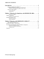
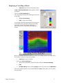
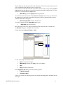
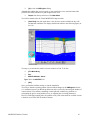
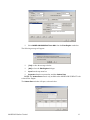
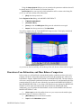
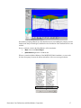
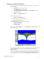
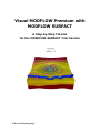
Visual MODFLOW Premium with
MODFLOW SURFACT
A Step-by-Step Tutorial
for the MODFLOW-SURFACT Trial Version
© Waterloo Hydrogeologic
TABLE OF CONTENTS
Introduction. . . . . . . . . . . . . . . . . . . . . . . . . . . . . . . . . . . . . . . . . . . . . . 2
Benefits of MODFLOW-SURFACT . . . . . . . . . . . . . . . . . . . . . . . . . . . . . . . . . . . . . . . . . 2
MODFLOW-SURFACT Interface in Visual MODFLOW . . . . . . . . . . . . . . . . . . . . . . . . . . . . . . . . . . . 2
Limitations of the MODFLOW-SURFACT Trial Version . . . . . . . . . . . . . . . . . . . . . . . . . . . . . . . . . . . 2
How to Use this Tutorial. . . . . . . . . . . . . . . . . . . . . . . . . . . . . . . . . . . . . . . . . . . . . . . . . . . 3
Terms and Notations. . . . . . . . . . . . . . . . . . . . . . . . . . . . . . . . . . . . . . . . . . . . . . . . . . . . . . . . . . . . . . . . . 3
Getting Started . . . . . . . . . . . . . . . . . . . . . . . . . . . . . . . . . . . . . . . . . . . . . . . . . . . . . . . . . . . . . . . . . . . . . 3
Module 1: Running the Simulation with MODFLOW-2000 . . . . . . 3
Running the Simulation . . . . . . . . . . . . . . . . . . . . . . . . . . . . . . . . . . . . . . . . . . . . . . . . . . . . . . . . . . . . . . 3
Output Visualization . . . . . . . . . . . . . . . . . . . . . . . . . . . . . . . . . . . . . . . . . . . . . . . . . . . . . . . . . 4
Displaying a Color Map of Heads . . . . . . . . . . . . . . . . . . . . . . . . . . . . . . . . . . . . . . . . . . . . . . . . . . . . . . 5
Modifying Pumping Wells . . . . . . . . . . . . . . . . . . . . . . . . . . . . . . . . . . . . . . . . . . . . . . . . . . . . 6
Running the Simulation . . . . . . . . . . . . . . . . . . . . . . . . . . . . . . . . . . . . . . . . . . . . . . . . . . . . . . . . . . . . . . 6
Output Visualization. . . . . . . . . . . . . . . . . . . . . . . . . . . . . . . . . . . . . . . . . . . . . . . . . . . . . . . . . . . . . . . . . 6
Module 2: Running with MODFLOW-SURFACT . . . . . . . . . . . . . 11
Why MODFLOW-SURFACT? . . . . . . . . . . . . . . . . . . . . . . . . . . . . . . . . . . . . . . . . . . . . 11
MODFLOW-SURFACT Run Options . . . . . . . . . . . . . . . . . . . . . . . . . . . . . . . . . . . . . . . . . . 11
Drawdown Cone Delineation, and Mass Balance Comparison . . . . . . . . . . . . . . . . . . . . . . . 14
Simulation with MODFLOW-2000 . . . . . . . . . . . . . . . . . . . . . . . . . . . . . . . . . . . . . . . . . . . . . . . . . . . . 16
Simulation with MODFLOW-SURFACT . . . . . . . . . . . . . . . . . . . . . . . . . . . . . . . . . . . . . . . . . . . . . . . 18
Visualizing in 3D . . . . . . . . . . . . . . . . . . . . . . . . . . . . . . . . . . . . . . . . . . . . . . . . . . . . . . . . . . . . . . . . . . 20
Summary . . . . . . . . . . . . . . . . . . . . . . . . . . . . . . . . . . . . . . . . . . . . . . . . . . . . . . . . . . . . . . . . . 22
© Waterloo Hydrogeologic
Introduction
This document contains a step-by-step tutorial to illustrate the capabilities of the
MODFLOW-SURFACT Flow Engine. This tutorial will guide you through the steps required
to:
• Modify and Run a flow simulation using the MODFLOW-2000 Flow Engine, and
inspect the output
• Modify and Run the same simulation using the MODFLOW-SURFACT Flow
Engine, and compare the output to the MODFLOW-2000 simulation
NOTE: You must have Visual MODFLOW Standard or higher to be able to use this tutorial.
NOTE: Some features described in this tutorial are only available in Pro or Premium
versions.
This tutorial assumes that you are already familiar with the Visual MODFLOW interface, and
with the process of building a groundwater model. If you are not familiar with Visual
MODFLOW, it is recommended that you work through the Visual MODFLOW
demonstration tutorial first.
Benefits of MODFLOW-SURFACT
The key benefits of MODFLOW-SURFACT for flow simulations are highlighted below:
• Handles complete desaturation and resaturation of grid cells
• Capable of modeling the movement of water through the Vadose Zone
• Accurate delineation and tracking of water table position, taking into account flow in
the unsaturated zone, delayed yield, and vertical flow components
• Automatic and correct redistribution of the total flow rate of a well screened through
multiple model layers when the upper cell(s) are pumped dry
• Accommodation of well-bore storage, and overpumped wells
• Prevents water table buildup beyond a specified recharge-ponding elevation
• Handling of seepage face boundary conditions
• Adaptive time-stepping schemes automatically adjust time-step size to the nonlinearities of the system, to optimize the solution stability
• Robust and efficient Pre-conditioned Conjugate Gradient matrix solver
• Capability of modeling unsaturated water or air movement
• Enhanced Newton-Raphson linearization option increases robustness for unconfined
and/or unsaturated flow conditions
MODFLOW-SURFACT Interface in Visual MODFLOW
Currently, Visual MODFLOW supports a graphical user interface for the Flow component of
MODFLOW-SURFACT. Transport simulations are not supported when using the
MODFLOW-SURFACT Flow Engine.
Limitations of the MODFLOW-SURFACT Trial Version
The Trial version of the MODFLOW-SURFACT Flow Engine is restricted to:
• A model size of 50 rows by 50 columns by 5 layers
• A maximum of 5 stress periods and 50 time steps
The fully licensed version of MODFLOW-SURFACT is capable of working with the normal
(default) grid size of Visual MODFLOW models, and with any custom grid developed for
Visual MODFLOW by Waterloo Hydrogeologic
MODFLOW Surfact Tutorial
2
How to Use this Tutorial
This tutorial is divided into two modules, and each module contains a number of sections.
Each section is written in an easy-to-use step-wise format. The modules are arranged as
follows.
Module 1 - Running MODFLOW-2000 and Output Visualization
Module 2 - Running MODFLOW-SURFACT and Output Visualization
Terms and Notations
For the purposes of this tutorial, the following terms and notations will be used:
Type:- type in the given word or value
Select:- click the left mouse button where indicated
- press the <Tab> key
↵
- press the <Enter> key
- Click the left mouse button where indicated
- double-click the left mouse button where indicated
[...]
- denotes a button to click on, either in a window, or in the menu bars.
The bold faced type indicates menu or window items to click on, or values to type in.
Getting Started
To start this tutorial:
(the Visual MODFLOW program icon) to start the Visual MODFLOW
program
File>Open from the Main Menu
Browse to the location of the tutorial files. From this folder, select the Airport-Surfact.vmf
file, and
[Open]
The Airport-Surfact model is already built and ready to run.
Module 1: Running the Simulation with MODFLOW-2000
Module 1 guides you through the run of a simulation using MODFLOW-2000.
[Run] from the Main Menu
Running the Simulation
[Run] from the Top Menu bar
An Engines to Run dialog box will appear listing the available Numeric Engines (as shown
in the figure below).
3
In the Engines to Run dialog, select the following options:
MODFLOW-2000
[Translate & Run]
Visual MODFLOW will then Translate the Visual MODFLOW data set into the standard
data input files required for the selected Numeric Engines, and then Run the simulations in a
separate window labelled VMEngines.
Output Visualization
Once the model has converged, you may [Close] the VMEngines window.
Output from the top menu bar of the Main Menu
Upon entering the Output section, Visual MODFLOW will automatically load the available
Output files for Head (.HDS) for all output times. Once these data files are loaded, the Output
screen will appear.
MODFLOW Surfact Tutorial
4
Displaying a Color Map of Heads
[Options] button from the left-hand tool bar
A C(O) - Head Equipotentials contour options window
will appear.
Click on the [Color Shading] tab.
The contour options dialog box should appear as shown
on the right.
Use Color Shading
[OK] to accept these settings
A color map of the head equipotentials for the top layer
of the model will be plotted according to the default
color scale selected. Note that the color map is
translucent in order to show the underlying model
features.
Before you continue with this exercise, turn-off the color shading option to avoid the screen
refresh times required to redraw the colormap.
[Options] from the left toolbar
Click on the [Color Shading] tab.
Remove the checkmark
from the checkbox
beside Use Color Shading
[OK]
[F10 Main Menu] button, and then [Input] from the top menu bar of the Main Menu
You will be transferred back to the Visual MODFLOW Input section where you can modify
the model input.
Output Visualization
5
Modifying Pumping Wells
Now that we have established a baseline for the simulation, we will modify the pumping
wells to show how dry cells create model convergence problems for MODFLOW-2000.
Wells/Pumping Wells from the top menu bar
[Edit Well] from the left toolbar.
Move the cursor to the Supply Well2 (located in the lower-right) and left-click to edit the
well.
An Edit Well window will appear. Supply Well2 is the second row in the well table (indicated
in the figure below). In this row, remove the checkmark from the Active column to
deactivate this pumping well.
Now select Supply Well1 from the well
table by placing your cursor in the first
row of the well table.
To change the Screened Intervals:
Click in the column labelled Screen Top
and enter the following values:
Well Table
Screen Top (m):14.0
Screen Bottom (m):0.3
Change the pumping Rate (m^3/day) to
-780,
[OK] to accept these changes
[F10 Main Menu], and then
click [Yes] to save your changes and return to the Main Menu.
Running the Simulation
To continue with the run options:
[Run] from the Main Menu options
[Run] from the Top Menu bar
In the Engines to Run dialog, select the following options.
MODFLOW-2000
[Translate & Run]
Visual MODFLOW will then Translate the Visual MODFLOW data set and Run the
simulation.
Output Visualization
Once the model has converged, you may [Close] the VMEngines window.
[Output] from the top menu bar of the Main Menu
MODFLOW Surfact Tutorial
6
You will be transferred to the Visual MODFLOW Output section where you will view the
new simulation results. This section provides instructions on displaying the de-saturated
conditions (i.e. dry cells).
Upon entering the Output section, Visual MODFLOW will automatically load the available
Output files for Heads (.HDS) and the Output screen will appear as shown below:
[View Row] from side menu bar, and then move your cursor onto the model region.
Click on a row to show the cross-section with the cone of depression around the pumping
well, and dry cells. The display should look similar to the following figure (row 30).
Modifying Pumping Wells
7
The profile shows that the water table is still within the well screen, but note that the top cell
of the well has dried out indicated by olive-colored cells.
Once you have viewed the results from your model, return to a plan view by clicking the View
Layer button, then moving your cursor onto the model region and clicking on layer 1. Then,
return to the Visual MODFLOW Input menu:
[Main Menu], and then [Input] from the top menu bar
You will be transferred back to the Visual MODFLOW Input section where you will increase
the pumping rate, causing the water table to drop below the layer bottom, thereby causing
problems with model convergence.
Wells>Pumping Wells from the Top Menu bar
You will be transferred to the Pump Wells input screen.
[Edit Well] from the left toolbar.
Move the cursor to the active supply well (Supply Well1) and left-click to edit the well.
An Edit Well dialog box will appear. In this window:
Change the pumping Rate (m^3/day) to -1200.
To save your changes and run the model:
[OK] to accept these changes
[Main Menu], and then click [Yes] to save your changes
[OK]
[Run] from the Top Menu bar
In the Engines to Run dialog, select the following options:
MODFLOW-2000
[Translate & Run]
After a few seconds, the following message will appear indicating that the simulation has not
converged.
MODFLOW Surfact Tutorial
8
.
[OK] to close the dialog.
Expand the solver iteration window so you can see the VMEngine window as shown below.
Note that the maximum number of outer iterations (50) has been reached without satisfying
the head change criterion, and a “Stop: no convergence!” message is displayed at the end.
(Show files) icon, and an Open window will appear. In this window, select
AIRPORT-SURFACT.LST and click Open to view the Listing file.
Scroll down to examine the “Cell conversions for iter.=” entries (starting approximately 1/4
through the file), when MODFLOW converts a cell from wet to dry or vice versa. You can see
that some cells in layer 1, rows 29-32 are dry, which is preventing the model convergence.
Modifying Pumping Wells
9
[X] to close the VMEngines dialog.
Although the solution has not converged, we can examine the cross-sectional water table
profile of the failed simulation to gain insight into the issue.
Output from the top menu bar of the Main Menu
You will be transferred to the Visual MODFLOW Output section.
[View Row] from side menu bar to view the cross-section with the the dry cells
(desaturated condition).The display should look similar to the following figure (at
row 30).
You may try to increase the number of outer iterations to 500. To do this
[F10 Main Menu]
Run
MODFLOW 2000 - Solver
Type: 500 in the MXITER field
[OK]
Once you finished with the settings, re-run the simulation.
You will see that the repeating pattern of head residual changes in the VMEngines window
(i.e. oscillation) assures you that the problem can not be resolved by increasing the number of
outer iterations. You could try smoothing out the hydraulic conductivity gradients, or
redesigning the grid, or using another solver, or adjusting the re-wetting parameters.
However, with high pumping rates, the problem of dry cells often cannot be avoided. In such
a situation, we need to look for another solution.
MODFLOW Surfact Tutorial
10
Module 2: Running with MODFLOW-SURFACT
Why MODFLOW-SURFACT?
Using the MODFLOW-2000 Engine, a multi-layer well is represented as a group of single
layer wells, and fails to take into account the inter-connection between various layers
provided by the well. One of the most significant problems related to this approach is that
well grid cells are essentially “shut off” when the water table drops below the bottom of the
grid cell (i.e. when the grid cell becomes dry). This reduces the total pumping rate of the well
(as the rate is distributed between all the screened cells initially), and may cause the water
table to “rebound” and re-activate the dry well grid cell. This type of on-again-off-again
behavior for the pumping well(s) causes the solution to oscillate, and may prevent the model
from converging to a solution. In the event the model does converge to a solution, the model
results may be misleading if one or more pumping wells have lower than expected total
pumping rates.
This issue can be addressed by selecting the MODFLOW-SURFACT Engine for Flow. In
contrast to the standard MODFLOW Engines, MODFLOW-SURFACT is able to
dynamically redistribute pumping rates to the remaining active grid cells if one or more cells
in the screened interval goes dry, thereby more accurately simulating the real-world effects of
partial overpumping of a well screened over multiple layers.
In view of the serious difficulties encountered with the previous increased pumping rate
simulation, an approach is required that allows free movement of the water table in the
unconfined layers without any kind of forced convergence. The MODFLOW-SURFACT
Flow Engine is capable of modeling unsaturated moisture, and couple the surface-water and
groundwater flow regimes. It utilizes special numerical methods and powerful solvers to
avoid the solution convergence problems caused by dry cells. A brief description of the
MODFLOW-SURFACT capabilities is provided in Appendix-C of the Visual MODFLOW
User’s Manual.
Module 2 will guide you through the selection of the MODFLOW-SURFACT Flow Engine,
and show you how a solution for a model with dry cell problems can be obtained.
MODFLOW-SURFACT Run Options
In this section, you will select MODFLOW-SURFACT as the Flow Numeric Engine, and rerun your model.
[Main Menu] located on the bottom toolbar
Setup/Edit Engines from the top menu bar
The following Edit Engines dialogue will appear.
MODFLOW-SURFACT Run Options
11
Select MODFLOW-SURGFACT from HGL from the Flow Engine combo box
The following message will appear:
[Yes] to close the message window
[OK] to close the Edit Engines dialogue
Input from the top menu bar
Properties from the top menu bar, and then Vadose Zone
NOTE: The Vadose Zone menu is only available when MODFLOW-SURFACT is the
selected Flow Engine.
The Vadose Zone window will open, as shown below:
MODFLOW Surfact Tutorial
12
From this window you may select different simulation types, as listed below, and customize
hydraulic properties of the porous media and phase constants:
•
•
•
•
•
Groundwater flow (Pseudo-soil function)
Groundwater flow (van Genuchten)
Groundwater flow (Brooke-Corey)
Soil Vapor flow (van Genuchten)
Soil Vapor flow (Brooke-Corey)
In this tutorial, the Groundwater flow (Pseudo-soil function) simulation type will be used.
If this option is not already selected, click the pull-down menu and select it from the list. It
simulates 3-D variably saturated flow, and can easily handle unconfined saturatedunsaturated moisture movement.
[OK] to close the Vadose Zone window
[F10 Main Menu] located on the bottom toolbar
[Run] from the Main Menu options
You will be transferred to the Visual MODFLOW Run section.
Prior to running the model, in the Run section, you could customize the default run-time
settings for MODFLOW-SURFACT including:
Time-steps for each stress period. This option is activated only when transient flow is
simulated. MODFLOW-SURFACT includes “adaptive-time stepping” schemes with
automatic generation and control of time steps to efficiently perform transient simulations.
Initial Heads provide the reference elevations for the heads in steady state solution, and
can reduce the required run time significantly.
Solver selection and settings. Note that PCG4 is specially designed for MODFLOW-
SURFACT. PCG4 is a simple, robust, and efficient solver, which requires less computer
resources than the PCG2 solver in MODFLOW.
Under the Recharge settings, in addition to Recharge options for MODFLOW,
MODFLOW-SURFACT allows you to simulate a Seepage Face Boundary Condition. In this
tutorial, the “Recharge is applied to the uppermost active layer” option is selected.
Layers settings are used to set the Interblock transmissivity and Layer type. The two
settings are combined to make up the LAYCON value which is used by the numeric engines.
Note that in MODFLOW-SURFACT the variably saturated flow options are implemented
with Value 40 and 43 for all layers in the model grid (as shown below)
Rewetting settings are used to specify the conditions under which Dry Cells will become
Wet again.
Anisotropy dialogue allows you to set the horizontal anisotropy by layer.
MODFLOW-SURFACT Run Options
13
Using the Output Control dialogue you can customize the parameters and times that will
be printed into the .LST file and/or saved to the binary file.
List File Opt allows you to specify which information will be written to the listing file
(.LST), as well as the format of this information.
[Run] from the top menu bar
In the Engines to Run dialog, select MODFLOW-SURFACT.
MODFLOW-SURFACT
[Translate & Run]
[Close] to close the VMEngines dialog once the solution has converged.
Output from the top menu bar of the Main Menu
You will be transferred to the Visual MODFLOW Output section. The display should look
similar to the following figure (row 30).
As you can see, there are still dry cells at the top of the well, however the model converged.
Drawdown Cone Delineation, and Mass Balance Comparison
In this section you will modify the constant head boundary conditions and move the active
pumping well to the center of the model. You will increase the pumping rate, and then run
both Numeric Engines: MODFLOW-SURFACT and MODFLOW-2000. The input changes
will create a steep hydraulic gradient (drawdown) around the well, and demonstrate how the
pumping-induced dry cells are more realistically represented with MODFLOW-SURFACT
than with MODFLOW-2000 (i.e. the shape of the drawdown cone obtained by MODFLOWSURFACT will be much smoother than the shape obtained by MODFLOW-2000).
Additionally, you will compare the Mass Balance results from the MODFLOW-2000 and
MODFLOW-SURFACT runs.
[View Layer] on the side toolbar, then move your cursor onto the model region,
and click on Layer 1 to return to a Plan View.
[Main Menu] located on the bottom toolbar
Input from the Main Menu options
MODFLOW Surfact Tutorial
14
Now you will move the active pumping well (Supply Well1) from its existing location to the
center of the model grid.
Wells/Pumping Wells from the top menu bar
To move the pumping well to the center of your model:
[Move Well]
Move the cursor to the top left pumping well and left-click to select the well, then move the
cursor to the center of the model and left-click to move the pumping well to the new location.
[Edit Well] from the Side Menu bar
Click on the well at it’s new location, and an Edit Well window will appear (shown below).
Enter the following information in the top row of the well table (Supply Well1):
X:
975
Y:
1020
To modify the Screened Intervals, click in the column labelled Screen Top and enter the
following values:
Screen Top (m):14.0
Screen Bottom (m):1.29
In the Pumping Schedule frame, leftclick inside the text box under the column
labelled Rate and enter the following
information:
Rate (m^3/day): -3000
[OK] to accept this well
information
Next you will modify the Constant Head
boundary conditions assigned along the
north boundary.
Use the overlay picklist on the left-hand
toolbar to switch from the Pump Wells to
the Const. Head overlay (scroll through
the list to find Const. Head).
[Yes] to save your changes
[Edit>] Group from the left hand toolbar. A Constant-Head - [Edit Group]
window will appear.
The brown colored cells at the top of the model and they will be highlighted in pink
Change the head values by clicking in the Start Time Head column, then editing the
“$SHEAD” text that appears above the column heading. Repeat for the “$EHEAD” text:
Start Time Head (m): 18
Stop Time Head (m): 18
[OK] to accept these values
The pink line of grid cells will turn back to a brown color, indicating that the Constant Head
boundary condition has been changed for these cells.
Drawdown Cone Delineation, and Mass Balance Comparison
15
Simulation with MODFLOW-2000
You will first run MODFLOW-2000 to see the effect of the input changes:
[Main Menu] located on the bottom toolbar
[Yes] to save your changes
Setup/Edit Engines from the top menu bar
MODFLOW-2000 from the Flow Engine combo box
[Yes] in the message
[OK]
To continue with the run options:
[Run] from the Main Menu options
You will then be transferred to the run options screen:
Run from the top menu bar
In the Engines to Run dialog, select the following options:
MODFLOW-2000
[Translate & Run]
After a few seconds the following message will appear:
.
Although the solution has not converged, we can examine the cross-sectional water table
profile of the failed simulation to gain insight into the issue.
[OK] to close the dialog box, and [Close] the VMEngines window
[Output] from the Top Menu bar of the Main Menu
You will be transferred to the Visual MODFLOW Output section. Visual MODFLOW will
automatically load the available Output files for Head (.HDS).
Click [View Row], and move your cursor onto the model region. Click to select a crosssection view, and the Output screen will similar to the screenshot below (row 20):
MODFLOW Surfact Tutorial
16
Note that the pumping induced dry cells (drawdown cone) surrounding the pumping well are
limited to the shape of model grid, and therefore the distribution of the desaturated zone is not
realistic.
Next we will take a look at the Mass Balance of this simulation:
Maps, then select Zone Budget
[Mass Balance] from the Left Menu bar
When we examine the Mass Balance of the MODFLOW-2000 simulation, we can see the
obvious discrepancy between the inflow and outflow of the non-converged solution.
Drawdown Cone Delineation, and Mass Balance Comparison
17
Simulation with MODFLOW-SURFACT
Now we will switch to the MODFLOW-SURFACT Flow Engine to see if we can obtain
model convergence:
Main Menu located on the bottom toolbar
Setup/Edit Engines from the top menu bar
Select MODFLOW-SURFACT from HGL from the Flow Engine combo box
[Yes] in the message
[OK] to close the Edit Engines window
To continue with the run options:
[Run] from the Main Menu options
You will then be transferred to the run options screen:
Run from the top menu bar
In the Engines to Run dialog, select the following options:
MODFLOW-SURFACT
[Translate & Run]
When your model has successfully converged, click Output menu and the Output screen will
appear as shown below (row 20):
Note that the pumping induced desaturation surrounding the pumping well is represented by a
smooth-shaped drawdown cone, which is more realistic than the one simulated by
MODFLOW-2000.
Note: You will notice in cross section that the cone of depression drops below the bottom of
the well screen. This is because the general well package was used for this simulation. To
achieve even more realistic output, select the Fractured Linear Well (FLW4) packge in the
MODFLOW Surfact Tutorial
18
run settings. With this well package, the cone of depression will not drop below the bottom of
the well screen.
When we examine the Mass Balance of the MODFLOW-SURFACT simulation (by clicking
on Maps - Zone Budget from the Top Menu bar, then clicking on [Mass Balance] from the
Left Menu bar), we can see that the percent discrepancy is much better, indicating we have a
much more accurate solution. Since MODFLOW-SURFACT can automatically redistribute
pumping rates when well cells go dry, a more accurate flow calculation can be made.
If time permits, you may also want to experiment with the well packages available through
the Engines to Run window. Before running the model, you can select the Advanced
options, and select the User Defined Settings option, as shown in the following screenshot.
By clicking on the
button, the Packages window will open , as shown in the following
Drawdown Cone Delineation, and Mass Balance Comparison
19
screenshot, where you can switch between the standard well package, and the FWL4 package.
As described in the MODFLOW-SURFACT User’s Manual (Chapter 3), the FWL4 package
was designed to overcome several problems associated with the original WEL1 package. One
important feature added to the FWL4 package is the ability to adjust total well withdrawal
when the water level in the well has reached the well bottom. In situations where a partially
penetrating well is being pumped beyond its capacity, the WEL1 package incorrectly
continues its calculations and allows head values to drop below the well-bottom elevation. In
other situations, the WEL1 package can cause the model to become unstable by cyclically
drying and wetting the pumping cells between iterations.
Please NOTE that the FWL4 package will only function with 1 pumping well in the model. If
you choose to experiment with this package, you will need to delete the second (inactive)
pumping well before running the simulation.
To continue with the rest of the tutorial, please see the following section describing the use of
the Visual MODFLOW 3D Explorer.
Visualizing in 3D
Now that you have examined the model in various 2D views, you can visualize it in 3D. To do
so,
[F2 3D] button on the bottom toolbar
The 3D Explorer window will load as shown below:
MODFLOW Surfact Tutorial
20
To display the depression cone
[+] beside Output
Right-click on Drawdown and select Create Isosurface
The following dialogue will load:
Show Borders
Color from Palette
type: 0 for the Isosurface value
[OK]
Use the Navigation Tools at the bottom of the model to position the grid so that you can
clearly see the depression cone:
Drawdown Cone Delineation, and Mass Balance Comparison
21
You can also display the dry cells. To do so:
[+] beside Heads
Dry Cells
Visible in the Properties frame
Feel free to experiment with other features of the 3D Explorer.
Summary
In this tutorial we have shown that model convergence difficulties arise when attempting to
simulate the hydrogeological environment using the standard MODFLOW code. The steep
hydraulic gradients surrounding the pumping well posed problems within the unsaturated
zone of the model. The pseudo-soil function of MODFLOW-SURFACT was chosen to
account for the saturated and unsaturated processes within the model, as it avoids the wet/dry
non-linear iterations of standard MODFLOW. The main benefit of MODFLOW-SURFACT is
that the user is able to focus on their model calibration, rather than model stability.
The major features of MODFLOW-SURFACT when coupled with Visual MODFLOW
include:
• Extending the capability of Visual MODFLOW to handle Vadose Zone and Vapor
flow simulations
• Greater stability and faster model convergence with complex solutions
• Accurate handling of pumping wells screened across multiple layers
These features make MODFLOW-SURFACT an excellent addition to the Visual
MODFLOW modeling package.
MODFLOW Surfact Tutorial
22
Summary
23