1
FALL3D-6.2 User Guide Arnau Folch1, Antonio Costa2 1 Earth Sciences Division Barcelona Supercomputing Center - Centro Nacional de Supercomputación Edifici Nexus II - c/ Jordi Girona 29 08034 Barcelona, Spain 2 Istituto Nazionale di Geofisica e Vulcanologia Via Diocleziano 328 - 80124 Napoli, Italy March 2010 2 FALL3D 6.2 USER’S MANUAL Contents 1 Introduction 2 Ash 2.1 2.2 2.3 2.4 2.5 2.6 transport model Governing equations . . Eddy Diffusivity Tensor Settling velocity models Meteorological variables Source term . . . . . . . Particle aggregation . . 3 . . . . . . . . . . . . . . . . . . . . . . . . . . . . . . . . . . . . . . . . . . . . . . . . . . . . . . . . . . . . . . . . . . . . . . . . . . . . . . . . . . . . . . . . . . . . . . . . . . . . . . . . . . . . . . . . . . . . . . . . . . . . . . . . . . . . . . . . . . . . . . . . . . . . . . . . . . . . . . . . . . . . . . . . . . . . . . . . . . . . . . . . . . . . . . . . . . . . . . . . . . . . . . . . . . . . . . . . . . . . . . 3 Overview of the program FALL3D-6.2 3 3 3 5 6 6 6 6 4 The FALL3D-6.2 Input files 4.1 The control file filename.inp . . . 4.1.1 BLOCK TIME UTC . . . . . 4.1.2 BLOCK GRID . . . . . . . . 4.1.3 BLOCK FALL3D . . . . . . . 4.1.4 BLOCK GRANULOMETRY 4.1.5 BLOCK SOURCE . . . . . . 4.1.6 BLOCK OUTPUT . . . . . . 4.2 The database file filename.dbs.nc 4.3 The granulometry file filename.grn 4.4 The source file filename.src . . . 4.5 The points file filename.pts . . . . . . . . . . . . . . . . . . . . . . . . . . . . . . . . . . . . . . . . . . . . . . . . . . . . . . . . . . . . . . . . . . . . . . . . . . . . . . . . . . . . . . . . . . . . . . . . . . . . . . . . . . . . . . . . . . . . . . . . . . . . . . . . . . . . . . . . . . . . . . . . . . . . . . . . . . . . . . . . . . . . . . . . . . . . . . . . . . . . . . . . . . . . . . . . . . . . . . . . . . . . . . . . . . . . . . . . . . . . . . . . . . . . . . . . . . . . . . . . . . . . . . . . . . . . . . . . . . . . . . . . . . . . . . . . . . . . . . . . . . . . . . . . . . . . . . . . . . . . . . . . . . . . . . . . . . . . . . . . . . . . . . . . . . . . . . 7 7 8 8 9 9 10 11 11 12 12 13 5 Program Setup 5.1 Installation . . . . . . . . . . . 5.1.1 Unix/Linux/Mac X OS 5.1.2 Windows OS . . . . . . 5.2 Execution . . . . . . . . . . . . 5.2.1 Unix/Linux/Mac X OS 5.2.2 Windows OS . . . . . . . . . . . . . . . . . . . . . . . . . . . . . . . . . . . . . . . . . . . . . . . . . . . . . . . . . . . . . . . . . . . . . . . . . . . . . . . . . . . . . . . . . . . . . . . . . . . . . . . . . . . . . . . . . . . . . . . . . . . . . . . . . . . . . . . . . . . . . . . . . . . . . . . . . . . . . . . . . . . . . . . . . . . . . . . . . . . . . . . . . . 13 13 13 13 13 14 14 Appendices Appendix A: Format of the meteo profile file (filename.profile) . . . . . . . . . . . . . . . . Appendix B: The GRD format . . . . . . . . . . . . . . . . . . . . . . . . . . . . . . . . . . . . Appendix C: The NetCDF format . . . . . . . . . . . . . . . . . . . . . . . . . . . . . . . . . . 14 14 15 15 . . . . . . . . . . . . . . . . . . FALL3D 6.2 USER’S MANUAL 1 3 Introduction FALL3D-6.2 is a 3-D time-dependent Eulerian model for the transport and deposition of volcanic ash. The model solves the advection-diffusion-sedimentation (ADS) equation on a structured terrain-following grid using a second-order Finite Differences (FD) explicit scheme. Different parameterizations for the eddy diffusivity tensor and for the particle terminal settling velocity can be chosen. The code, written in FORTRAN-90, is available for Unix/Linux/Mac X Operating Systems (OS). A set of pre- and postprocess utility programs and OS-dependent scripts to launch them are also included in the FALL3D-6.2 distribution package. Although the model has been designed to forecast volcanic ash concentration in the atmosphere and ash loading at the ground, it can also be used to model the transport of other kinds of airborne solid particles. The model inputs are meteorological data, topography, grain-size distribution, shape and density of particles, and mass rate of particle injected into the atmosphere. The FALL3D-6.2 model can be used as a tool for short-term ash deposition forecasting and for volcanic fallout hazard assessment. FALL3D-6.2 is available in two versions called PUB (Public) version and PROF (Professional) version. More information on http://www.bsc.es/projects/earthscience/fall3d/ and http://datasim.ov.ingv.it/Fall3d.html 2 Ash transport model In this section we briefly describe the governing equations and the main assumptions used in FALL3D-6.2. For further details see Costa et al. (2006); Folch et al. (2009). 2.1 Governing equations The main factors controlling atmospheric transport of ash are wind advection, turbulent diffusion, and gravitational settling of particles. Neglecting particle-particle interaction effects (collisions, aggregation, etc.), the Eulerian form of the continuity equation written in a generalized coordinate system (X, Y, Z) is (Byun and Schere, 2006; Costa et al., 2006): ∂C ∂C ∂C ∂C ∂Vsj + VX + VY + (VZ − Vsj ) = −C∇ · V + C ∂t ∂X ∂Y ∂Z ∂Z ∂C/ρ∗ ∂C/ρ∗ ∂C/ρ∗ ∂ ∂ ∂ ρ∗ K X + ρ∗ K Y + ρ∗ K Z + S∗ + ∂X ∂X ∂Y ∂Y ∂Z ∂Z (1) where C is the transformed concentration, V = (VX , VY , VZ ) is the transformed wind speed, KX , KY and KZ are the diagonal terms of the transformed eddy diffusivity tensor, ρ∗ is the transformed atmospheric density, and S∗ is the transformed source term. FALL3D-6.2 solves Eq. (1) for each particle class j using a curvilinear terrain-following coordinate system (X = mx, Y = my, z → Z), where m is the map scale factor and Z = z − h(x, y), with h(x, y) denoting the topographic elevation, and (x, y, z) are the Cartesian coordinates. The scaling factors for this particular transformation are given in Table 1 (Byun and Schere, 2006). The generic particle class j is defined by a triplet of values characterizing each particle (dp , ρp , Fp ), that are, respectively, diameter, density, and a shape factor. For dp we use the equivalent diameter d, which is the diameter of a sphere of equivalent volume. For the shape factor Fp we choose the sphericity ψ, which is the ratio of the surface area of a sphere with diameter d to the surface area of the particle. In our approximation, each triplet (d, ρp , ψ) is sufficient to define the settling velocity. Effect of Earth’s curvature are considered when the lat-lon coordinate system is used through the Jacobian of the transformation. 2.2 Eddy Diffusivity Tensor In FALL3D-6.2 only the diagonal components of the Eddy Diffusivity Tensor, i.e. the vertical Kz and the horizontal Kh = Kx = Ky components, are considered. The available choices for describing the vertical component Kz are: 1. Option CONSTANT, i.e. Kz = constant, where the constant value is assigned by the user; 4 FALL3D 6.2 USER’S MANUAL Parameter Coordinates Horizontal Velocities Vertical velocity Diffusion Coefficients Concentration Density Source Term Scaling X = mx; Y = my; Z = z − h(x, y) VX = mvx ; VY = mvy i h ∂h (VZ − VSj ) = J −1 (vz − vsj ) − m vx ∂h ∂x + vy ∂y KX = Kx ; KY = Ky ; KZ ≃ Kz J −2 C = cJ/m2 ρ∗ = ρJ/m2 S∗ = SJ/m2 Table 1: Scaling factors for a terrain-following coordinate system (x = mX, y = mY, z → Z). (x, y, z) are the Cartesian coordinates, m the map scale factor (for the UTM coordinate system m = 1) and J is the determinant of the Jacobian of the coordinate system transformation. 2. Option SIMILARITY. In this case, evaluates Kz as: κu∗ z 1 − Kz = κu∗ z 1 − inside the Atmospheric Boundary Layer (ABL), FALL3D-6.2 −1 hz z 1 + 9.2 h Lh 1/2 z hz 1 − 13 h Lh h/L ≥ 0 stable h/L ≤ 0 unstable (2) where κ is the von Karman constant (κ = 0.4), u∗ is the friction velocity, h is the ABL height, and L is the Monin-Obukhov length (see Costa et al., 2006). The expression above comes from an extension of the Monin-Obukhov similarity theory to the entire ABL (Ulke, 2000). On the other hand, above the ABL (z/h > 1), Kz is considered a function of the local vertical wind gradient, a characteristic length scale lc , and a stability function Fc which depends on the Richardson number Ri: 2 ∂U Fc (Ri) (3) K z = lc ∂z q where U = yx2 + u2y . For lc and Fc , FALL3D-6.2 adopts the relationship used by the CAM-3.0 model (Collins et al., 2004): lc = 1 1 + κz λc 1 1 + 10Ri(1 + 8Ri) Fc (Ri) = √ 1 − 18Ri −1 stable (4) (Ri > 0) (5) unstable (Ri < 0) where λc is the so-called asymptotic length scale (λc ≈ 30m). The available choices for describing the horizontal component Kh = Kx = Ky are: 1. Option CONSTANT, i.e. Kh = constant, where the constant value is assigned by the user; 2. Option RAMS. In this case, a large eddy parameterization as that used by the RAMS model (Pielke et al., 1992) can be used for evaluating Kh : v " u 2 2 2 # u ∂vx ∂v ∂v ∂v y x y 2 +2 + + (6) Kh = P rt max km ; (CS ∆) t ∂y ∂x ∂x ∂y √ where P rt is the turbulent Prandtl number (typically P rt ≈ 1), km = 0.075∆4/3 , ∆ = ∆x∆y, ∆x and ∆y are the horizontal grid spacings, and CS is a constant ranging from 0.135 to 0.32. 5 FALL3D 6.2 USER’S MANUAL 3. Option CMAQ. In this case, the horizontal diffusion is evaluated as in the CMAQ model (Byun and Schere, 2006): 1 1 1 = + (7) Kh Kht Khn where: 2 Kht = α ∆x∆y s Khn 2 2 ∂vy ∂vx ∂vy ∂vx + − + ∂x ∂y ∂x ∂y ∆xf ∆yf = Khf ∆x∆y (8) (9) where α = 0.28 and the values of Khf and ∆xf = ∆yf depend on the algorithm. Using this parameterization, for a large grid size the effect of the transportive dispersion is minimized, whereas for a small grid size the numerical diffusion term is reduced (Byun and Schere, 2006). Thanks to the heuristic relationship (7), the smaller between Kht and Khn dominates. In our case we set Khf = 8000 m2 s−1 for ∆xf = ∆yf = 4 km and also a minimum value for Kh equal to km = 0.075∆4/3 was imposed. 2.3 Settling velocity models There are several semi-empirical parameterizations for the particle settling velocity vs if one assumes that particles settle down at their terminal velocity: s 4g (ρp − ρa ) d (10) vs = 3Cd ρa where ρa and ρp denote air and particle density, respectively, d is the particle equivalent diameter, and Cd is the drag coefficient. Cd depends on the Reynolds number, Re = dvs /νa (νa = µa /ρa is the kinematic viscosity of air, µa the dynamic viscosity). In FALL3D-6.2 different options are possible for estimating settling velocity, such as: 1. ARASTOOPOUR model (Arastoopour et al., 1982): 24 (1 + 0.15Re0.687 ) Re ≤ 988.947 Re Cd = 0.44 Re > 988.947 (11) valid for spherical particles only. 2. GANSER model (Ganser, 1993): Cd = o 24 n 0.6567 + 1 + 0.1118 (Re K1 K2 ) ReK1 0.4305K2 3305 1+ Re K1 K2 (12) 0.5743 where K1 = 3/[(dn /d) + 2ψ −0.5 ], K2 = 101.8148(−Logψ) are two shape factors (dn is the average between the minimum and the maximum axis, d is the equal volume sphere), and ψ is the particle sphericity (ψ = 1 for spheres). For calculating the sphericity is practical to use the concepts of operational and working sphericity, ψwork introduced by Wadell (1933); Aschenbrenner (1956), which are based on the determination of the volume and of the three dimensions of a particle respectively: (P 2 Q)1/3 p ψwork = 12.8 (13) 1 + P (1 + Q) + 6 1 + P 2 (1 + Q2 ) with P = S/I, Q = I/L, where L is the longest particle dimension, I is the longest dimension perpendicular to L, and S is the dimension perpendicular to both L and I. 6 FALL3D 6.2 USER’S MANUAL 3. WILSON model (Walker et al., 1971; Wilson and Huang, 1979) using the interpolation suggested by Pfeiffer et al. (2005): p 24 −0.828 Re ≤ 102 +2 1−ϕ Re ϕ 1 − Cd |Re=102 Cd = (14) 1− (103 − Re) 102 ≤ Re ≤ 103 900 1 Re ≥ 103 where ϕ = (b + c)/2a is the particle aspect ratio (a ≥ b ≥ c denote the particle semi-axes). 4. DELLINO model (Dellino et al., 2005): vs = 1.2605 0.5206 νa Ar ξ 1.6 d (15) where Ar = gd3 (ρp − ρa )ρa /µ2a is the Archimedes number, g the gravity acceleration, and ξ is a particle shape factor (sphericity to circularity ratio). It is recommended to not extrapolate this option for particle diameter beyond the range used in the experiments by Dellino et al. (2005). Since for FALL3D-6.2 the primary particle shape factor is the sphericity ψ, for sake of simplicity, ϕ in (14) and ξ in (15) are calculated approximating particles as prolate ellipsoids (the same approximation is used for estimating dn ). 2.4 Meteorological variables FALL3D-6.2 uses an off-line strategy, i.e. the meteorological variables are calculated independently by a different meteorological model or information, and interpolated to the spatial and temporal grid of FALL3D-6.2. FALL3D-6.2 reads time-dependent meteorological data (wind field, air temperature, Monin-Obukhov length L, friction velocity u∗ , and ABL height h) and topography from a database file in NetCDF format. This file can be created by an external utility program (SETDBS). This strategy allows FALL3D-6.2 to be used from micro- to meso-scale. In the PUB distribution version there are a few options to generate this database depending on the scale of application. For the possible choices see Section 4.2. 2.5 Source term FALL3D-6.2 reads the time-dependent source term (mass released per unit time at each grid point) from an external file. This file can be generated by the SETSRC utility program, as i) a point source, ii) imposing a mushroom-like shape (Suzuki option) or iii) by using a model based on the Buoyant Plume Theory (BPT; see Section 4.4). 2.6 Particle aggregation A subroutine describing particle aggregation in presence of water is being tested. Aggregation model and validation tests are presented in Costa et al. (2010); Folch et al. (2010). 3 Overview of the program FALL3D-6.2 FALL3D-6.2 needs the following input files: • An input file where control parameters and options are specified (filename.inp). This file is read by FALL3D-6.2 and the utility programs. • A database file in NetCDF format (see Appendix C) containing all meteorological data and the topography (filename.dbs.nc). • A granulometry file specifying the characteristics of the particles emitted into the atmosphere (filename.grn). FALL3D 6.2 USER’S MANUAL 7 • A source file specifying the discharge rates at the source points, typically along the eruptive column (filename.src). • Optionally, a file specifying a list of points (filename.pts) where tracking of variables is performed (e.g. to compute ash arrival times, accumulation rates, etc). The formats of the input files are described in Section 4. The FALL3D-6.2 package comes with a set of utility programs that can be used to generate the input files: • The utility SETDBS can be used to generate the database file filename.dbs.nc created in accord to the parameters specified in the blocks TIME UTC and GIRD of the input file filename.inp. This utility program reads meteo data from different sources and interpolates variables onto the FALL3D-6.2 computational grid. The time slice of the database must be equal or larger than the simulation time slice. • The utility SETGRN can be used to generate the granulometry file filename.grn in accord to the parameters specified in the block GRANULOMETRY of the input file filename.inp. This program generates only Gaussian and Bi-Gaussian distributions. For other distributions the user must provide the granulometry file. • The utility SETSRC can be used to generate the source file filename.src in accord to the parameters specified in the blocks TIME UTC and SOURCE of the input file filename.inp. The use of these utilities, although recommended, is not necessary if the user provides some of the necessary files directly. Once a simulation is concluded, FALL3D-6.2 outputs the following files: • The results file (filename.res.nc) in netCDF format. This file can be processed using several open-source programs (e.g. ncview, Panoply, ncl, etc.) to generate plots and animations. • The log file (filename.log) contains information about the run, including summary of input data, error and warning messages, etc. • The tracking points files (filename.pts.*) contain information about evolution of variables at the tracked points. There exist an output file for each point specified in the input file filename.pts. 4 The FALL3D-6.2 Input files 4.1 The control file filename.inp The control input file is an ASCII file made up with a set of blocks that define all the computational and physical parameters needed by FALL3D-6.2 and the rest of utility programs. Each program reads only the necessary blocks of the file. Parameters within a block are listed one per record, in arbitrary order, and can optionally be followed by one or more blank spaces and a comment. Maximum allowed lenght is 256 characters including comments. A detailed description of each record is given below. Real numbers can be expressed following the FORTRAN notation (e.g., 12e7 = 12 × 107 ). • BLOCK TIME UTC: Defines variables related to time. • BLOCK GRID: Defines the characteristics of the FALL3D-6.2 computational mesh. • BLOCK FALL3D: Defines the variables needed by FALL3D-6.2 program. • BLOCK GRANULOMETRY: Defines the variables needed by SETGRN program. • BLOCK SOURCE: Defines the variables needed by SETSRC program. • BLOCK OUTPUT: Defines the FALL3D-6.2 strategy for dumping of results. FALL3D 6.2 USER’S MANUAL 4.1.1 8 BLOCK TIME UTC This block of data defines variables related to time and is used by FALL3D-6.2 and by the utility programs SETDBS and SETSRC. • YEAR: Database starting year. • MONTH: Database starting month (1-12). • DAY: Database starting day (1-31). • BEGIN METEO DATA (HOURS AFTER 00): Time (in h after 0000UTC of the starting day) at which meteorological data starts in the database file. • TIME STEP METEO DATA (MIN): Time step (in min) of the meteo data in the database file. • END METEO DATA (HOURS AFTER 00): Time (in h after 0000UTC of the starting day) at which meteorological data ends in the database file. This time slice has to be larger than time slices defined by the records ERUPTION START (HOURS AFTER 00) and RUN END (HOURS AFTER 00). If not, the program will stop. • ERUPTION START (HOURS AFTER 00): Eruption start hours (after 0000UTC of the day). These are nt values (nt ≥ 1) that indicate the starting times of the different eruptive phases. Any type of transient behavior can be contemplated by adding a sufficient number of intervals. Eruptive conditions (plume height, MFR, etc.) are assumed constant during each phase (i.e. a quasi-steady approximation is used). The first value must be equal or larger than the value of the record BEGIN METEO DATA (HOURS AFTER 00). • ERUPTION END (HOURS AFTER 00) : Eruption end hour (after 0000UTC of the starting day). If the SETSRC program is used to generate the source term, this is the time slice at which source term is switched off (i.e. the time at which the last eruptive phase ends). • RUN END (HOURS AFTER 00): Run end hour (after 0000UTC of the starting day). Must be equal or lower than the value of the record END METEO DATA (HOURS AFTER 00). Note that, in general, a run should continue even when the source term is switched off (i.e. when the eruption has stopped) in order to allow the remaining airborne particles to sediment completely. 4.1.2 BLOCK GRID This block of data defines the variables needed by SETDBS program to generate the FALL3D-6.2 grid. Note that time and spatial coverage of the database must include the FALL3D-6.2 simulation interval. • COORDINATES: Defines the map projection. Possibilities are UTM or LON-LAT. Note that the UTM option can only be used if the domain is within a unique UTM zone. The use of the UTM coordinate system in large domains covering more than one UTM zone is not allowed (in this case, the LON-LAT option accounting for Earth’s curvature must be used instead). The sub-blocks UTM or LON LAT are read in each case respectively. • LONMIN: Minimum longitude (in decimal degrees) of the domain (i.e. longitude corresponding to the bottom left corner). Only used in the LON-LAT option. • LONMAX: Maximin longitude (in decimal degrees) of the domain (i.e. longitude corresponding to top right corner). Only used in the LON-LAT option. • LATMIN: Minimum latitude (in decimal degrees) of the domain (i.e. latitude corresponding to bottom left corner). Only used in the LON-LAT option. • LATMAX: Maximin latitude (in decimal degrees) of the domain (i.e. latitude corresponding to top right corner). Only used in the LON-LAT option. • LON VENT: Vent longitude. Only used in the LON-LAT option. • LAT VENT: Vent latitude. Only used in the LON-LAT option. FALL3D 6.2 USER’S MANUAL 9 • UTMZONE: UTM zone code in format nnL (e.g. 33S). Only used in the UTM option. • XMIN: minimum x-coordinate of the domain (bottom left corner). UTM coordinates must be given in m. Only used in the UTM option. • XMAX: maximum x-coordinate of the domain (top right corner). UTM coordinates must be given in m. Only used in the UTM option. • YMIN: minimum y-coordinate of the domain (bottom left corner). UTM coordinates must be given in m. Only used in the UTM option. • YMAX: maximum y-coordinate of the domain (top right corner). UTM coordinates must be given in m. Only used in the UTM option. • X VENT: x-coordinate of the vent. UTM coordinates must be given in m. Only used in the UTM option. • Y VENT: y-coordinate of the vent. UTM coordinates must be given in m. Only used in the UTM option. • NX: Number of grid nodes in the x-direction. • NY: Number of grid nodes in the y-direction. • ZLAYER (M): Array of heights (in m) of the vertical z-layers in terrain following coordinates. It is not necessary to specify the number of vertical layers since it is automatically calculated by the program. The vertical layers can be specified manually (as an array of values) or, for equally spaced vertical discretization, simply indicating the limits and the increment (e.g. FROM 0 TO 10000 INCREMENT 1000). 4.1.3 BLOCK FALL3D This block of data defines the variables needed by FALL3D-6.2 program. • TERMINAL VELOCITY MODEL: Type of terminal settling velocity model. Possibilities are ARASTOOPOUR, GANSER, WILSON, and DELLINO. • VERTICAL TURBULENCE MODEL: Type of model for vertical diffusion. Possibilities are CONSTANT or SIMILARITY. • VERTICAL DIFFUSION COEFFICIENT (M2/S): Value of the diffusion coefficient (in m2 /s). Only used if VERTICAL TURBULENCE MODEL = CONSTANT • HORIZONTAL TURBULENCE MODEL: Type of model for horizontal diffusion. Possibilities are CONSTANT, RAMS, or CMAQ. • HORIZONTAL DIFFUSION COEFFICIENT (M2/S): Value of the diffusion coefficient (in m2 /s). Only used if HORIZONTAL TURBULENCE MODEL = CONSTANT. • RAMS CS: Value of CS in the RAMS model (see eq. 6). Only used if HORIZONTAL TURBULENCE MODEL = RAMS. 4.1.4 BLOCK GRANULOMETRY This block of data defines the variables needed by SETGRN program. • DISTRIBUTION: Type of distribution. Possibilities are GAUSSIAN or BIGAUSSIAN. • NUMBER OF CLASSES: Number of granulometric classes. • FI MEAN: Mean value of Φ (Gaussian distribution). For Bi-Gaussian distributions two values must be provided. FALL3D 6.2 USER’S MANUAL 10 • FI DISP: Value of σ (Gaussian distribution). For Bi-Gaussian distributions two values must be provided. • FI RANGE: Minimum and maximum values of Φ (Φmin and Φmax respectively). • DENSITY RANGE: Values of densities ρmin and ρmax (in kg/m3 ) associated to Φmin and Φmax particles. Lineal interpolation is assumed. In particular, if ρmin = ρmax , density is constant for all classes. • SPHERICITY RANGE: Values of sphericity ψmin and ψmax associated to Φmin and Φmax particles. Lineal interpolation is assumed. In particular, if ψmin = ψmax , sphericity is constant for all classes. 4.1.5 BLOCK SOURCE This block of data defines the variables needed by the SETSRC program. This program generates the source term (eruptive column) for each of the nt ≥ 1 eruptive phases. • VENT HEIGHT: Height of the vent a.s.l. (in m). • SOURCE TYPE: Type of source distribution. Possibilities are POINT, SUZUKI or PLUME. In the case SOURCE TYPE = POINT only the sub-block POINT SOURCE is used: • MASS FLOW RATE (KGS): Array of values of the mass flow rate (in kg/s) for the nt eruptive phases. Alternatively, the user can use the word estimate and SETSRC automatically computes the MFR from the column heights based on empirical fits (Mastin et al., 2009). This is the typical situation during an eruption, when column height is likely to be the only observable available. • HEIGHT ABOVE VENT (M): Array of heights of the plume (in m above the vent) for the nt eruptive phases. Note that the plume heights must be lower than the top of the computational domain, specified in the record ZLAYER (M) of the GRID block. If not, the program will stop. In the case SOURCE TYPE = SUZUKI only the sub-block SUZUKI SOURCE is used: • MASS FLOW RATE (KGS): Array of values of the mass flow rate (in kg/s) for the nt eruptive phases. Alternatively, the user can use the word estimate and SETSRC automatically computes the MFR from the column heights based on empirical fits (Mastin et al., 2009). This is the typical situation during an eruption, when column height is likely to be the only observable available. • HEIGHT ABOVE VENT (M): Array of heights of the plume (in m above the vent) for the nt eruptive phases. Note that the plume heights must be lower than the top of the computational domain, specified in the record ZLAYER (M) of the GRID block. If not, the program will stop. • A: Array of values of the parameter A in the Suzuki distribution for the nt eruptive phases (Pfeiffer et al., 2005). • L: Array of values of the parameter λ in the Suzuki distribution for the nt eruptive phases (Pfeiffer et al., 2005). In the case SOURCE TYPE = PLUME only the sub-block PLUME SOURCE is used: • SOLVE PLUME FOR: Possibilities are MFR or HEIGHT. In the first case SETSRC solves for the mass flow rate given the column height, whereas in the second does the opposite. Since the plume equations use the mass flow rate as an input, the first option requires an iterative procedure. • MFR SEARCH RANGE: Two values n and m such that 10n and 10m specify the range of MFR values admitted in the iterative solving procedure (i.e. it is assumed that 10n ≤ M F R ≤ 10m ). Only used if SOLVE PLUME FOR=MFR. • MASS FLOW RATE (KGS): Values of the mass flow rate (in kg/s) for the nt eruptive phases. Only used if SOLVE PLUME FOR=HEIGHT. FALL3D 6.2 USER’S MANUAL 11 • HEIGHT ABOVE VENT (M): Heights of the plume (in m above the vent) for the nt eruptive phases. Note that the plume heights must be lower than the top of the computational domain, specified in the record ZLAYER (M) of the GRID block. Only used if SOLVE PLUME FOR=MFR. • EXIT VELOCIY (MS): Values of the magma exit velocity (in m/s) at the vent for the nt eruptive phases. • EXIT TEMPERATURE (K): Values of the magma exit temperature (in K) at the vent for the nt eruptive phases. • EXIT VOLATILE FRACTION (IN%): Values of the magma volatile at the vent for the nt eruptive phases in weight percent. 4.1.6 BLOCK OUTPUT This block of data defines the output strategy of the FALL3D-6.2 program. • POSTPROCESS TIME INTERVAL (HOURS): Postprocess time interval in hours. • POSTPROCESS 3D VARIABLES: Possibilities are YES or NO. If YES, FALL3D-6.2 writes 3D concentration in the output file filename.res.nc. If NO, only 2D variables are written to the output file. • POSTPROCESS CLASSES: Possibilities are YES or NO. If YES, FALL3D-6.2 writes results for all the classes. If NO, only total results are written. • TRACK POINTS: Possibilities are YES or NO. If YES, FALL3D-6.2 writes the tracking points files. 4.2 The database file filename.dbs.nc This file written in NetCDF format (see Appendix C) contains time-dependent meteorological data (wind field, air temperature and density, humidity, etc) needed by FALL3D-6.2. The file can be created by the external utility program SETDBS, which reads meteo data and interpolates to the FALL3D-6.2 space-time domain. There are a several options to generate this database depending on the scale of application. This strategy allows FALL3D-6.2 to be used from micro- to meso-scale. The possible choices are described below. • The simplest option consists of using a horizontally uniform wind derived from a vertical profile, typically obtained from sounding measurements or from indirect reconstructions. The vertical profile needs to be specified in the file filename.profile in the format described in the Appendix A. In this case, in addition to the profile filename.profile it is also necessary to furnish a topography file filename.top in GRD format (see Appendix B). • The second choice (CALMET option) uses data derived from the output of the meteorological diagnostic model CALMET (Scire et al., 2000). This option is used for assimilating and interpolating short-term forecasts (or re-analysis) from Mesoscale Meteorological Prognostic Models (MMPM) to a finer scale. In this case only the UTM coordinate system can be used. Note that the output of CALMET is a binary file that depends on the architecture of the machine were it was generated. Moreover note that this option is compatible only with a CALMET output time step equal to an hour (i.e., nsecdt=3600). • The third choice (NCEP-1 option) uses data from NCEP re-analysis 1 (see: http://www.esrl.noaa.gov/psd/data/gridded/data.ncep.reanalysis.html). • Other choices (available only in the PROF version) contemplate several global and mesoscale meteorological models such as ARPA-SIM, ETA, GFS, or NMMb. 12 FALL3D 6.2 USER’S MANUAL nc diam(1) rho(1) sphe(1) fc(1) ... diam(nc) rho(nc) sphe(1) fc(nc) Table 2: Format of the granulometry file filename.grn. 4.3 The granulometry file filename.grn The granulometry file is an ASCII file containing the definition of the particle classes (a class is characterized by particle size, density and sphericity). This file can be created by the utility program SETGRN. Note that SETGRN only generates distributions which are Gaussian or bi-Gaussian in ψ (log-normal in d) and linear in ρ and ψ. FALL3D-6.2 can handle more general distributions but, in this case, the granulometry file filename.grn has to be defined directly by the user. The file format is described in Table 2 and the meaning of the used symbols is the following: • nc: Number of particle classes. • diam: Class diameter (in mm). • rho: Class density (in kg/m3 ). • sphe: Class sphericity. • fc: Class mass fraction (0-1). It must verify that 4.4 P fc = 1. The source file filename.src The source file filename.src is an ASCII file containing the definition of the source term. The source can be defined for different time phases during which source values are kept constant. The number, position and values (i.e. Mass Flow Rate) of the source points can vary from one time slice to another and cannot overlap. There is no restriction on the number and duration of the time slices. It allows, in practise, to discretize any kind of source term. This file can be defined directly by the user, in the format described in Table 3, or created by using the utility program SETSRC. In the last case, the filename.src is created in accord to the parameter specified in the SOURCE block of the filename.inp. The options to be chosen in the filename.inp are i) a point source, ii) a mushroom-like shape (Suzuki option) or iii) an eruption column model based on the Buoyant Plume Theory (BPT). The format of the file filename.src is described in Table 3 and the meaning of the used symbols is the following: • itime1: Starting time of the time slice (in sec after 00UTC of the starting day). • itime2: End time of the time slice (in sec after 00UTC of the eruption starting day). • nsrc: Number of source points (can vary from one interval to another depending on the column height). • nc: Number of particle classes. • MFR: Mass flow rate (in kg/s). • x: Longitude or x-coordinate of the source isrc. • y: Latitude or y-coordinate of the source isrc. • z: z-coordinate of the source isrc above ground level (a.g.l.) (in m). • src: P Mass P flow rate (in kg/s) of each granulometric class for this point source. It must be verified that src(isrc, ic) = M F R. 13 FALL3D 6.2 USER’S MANUAL itime1 itime2 nsrc nc MFR x y z src(1,1) ... src(1,nc) ... x y z src(nsrc,1) ... src(nsrc,nc) Table 3: Format of the source file filename.src. Repeat this block for each time slice . 4.5 The points file filename.pts This file contains the names (identifiers) and coordinates of the points to be tracked. It is used only when the record TRACK POINTS in the input file filename.inp is set to YES. The format of the file filename.pts consists of lines (one line per point) with three columns specifying the point name, the point longitude (or x-coordinate if UTM coordinates are used), and the point latitude (or y-coordinate if UTM coordinates are used). There is no limit on the number of points. 5 Program Setup 5.1 Installation To install FALL3D-6.2 and the utility programs uncompress and untar the file Fall3d-6.2.PUB.tar.gz. It will create the folder structure shown in Table 4. The package contains the source codes, scripts, documentation, and a run examples. • For Unix/Linux/Mac X OS it is necessary to have a FORTRAN compiler and the NetCDF library (http://www.unidata.ucar.edu/software/netcdf/) already installed (version 3.6 or later). It is mandatory to compile FALL3D-6.2 using the same FORTRAN compiler that has been used to compile the NetCDF library. 5.1.1 Unix/Linux/Mac X OS For Unix/Linux/Mac X OS the package comes with an automatic installation script. Proceed as follows: 1. Enter the directory Install and edit the Install script file. Set up the variables HOMEFALL3D (FALL3D-6.2 home directory path), Lib netcdf (path of the NetCDF library in your computer), and COMPILER (name of the FORTRAN compiler). NOTE: Automatic installation is possible for the following standard compilers: gfortran, ifort, f90, xlf90. If you want to compile using a different compiler it is necessary to modify the Makefiles and the Scripts manually. 2. Run the Install script. This will compile FALL3D-6.2 and the utility programs, modify the scripts introducing your FALL3D-6.2 path and check the installation process. 3. Optionally, create an alias to the Script-manager file located in the folder Scripts. This script allows for launching FALL3D-6.2 and the utility programs directly from the command line. 5.1.2 Windows OS Not yet available for the current versions. 5.2 Execution To create a new run named problemname simply create a new directory problemname in the folder Runs, copy the control input file from the example run (rename it as problemname.inp), and modify it depending on your needs. 14 FALL3D 6.2 USER’S MANUAL Level 1 Fall3d Level 2 Documents Install Runs Scripts Sources ser Utilities Level 3 Run-name LibMaster SetDbs SetGrn SetSrc Description Contains the manual. Contains installation scripts. Contains the examples, one folder each. Contains the script files. FALL3D-6.2 sources (PUB version). Master library. SETDBS utility program. SETGRN utility program. SETSRC utility program. Table 4: Default structure of FALL3D-6.2 folders. 5.2.1 Unix/Linux/Mac X OS FALL3D-6.2 and the utility programs can be launched using the Script-manager with a series of arguments. It is recommended to use an alias for this script that can be called directly from any location (in the following it is assumed that the alias is Launch). From any location: • Type Launch SetGrn problemname to run the SETGRN utility program for problemname. • Type Launch SetDbs problemname meteo to run the SETDBS utility program for problemname. Here meteo is one of the following: profile/calmet62/ncep1. • Type Launch SetSrc problemname to run the SETSRC utility program for problemname. • Type Launch Pub problemname to run the PUB version of FALL3D-6.2 for problemname. 5.2.2 Windows OS Not yet available for the current versions. Appendices Appendix A: Format of the meteo profile file (filename.profile) For the profile option, the utility SetDbs needs an ASCII file containing the definition of the vertical wind profile and a topography file of the domain in GRD format (see Appendix B). In this case wind velocities are assumed constant on all the domain in a terrain-following coordinate system. The remaining variables are assumed with the values of the Standard Atmosphere. The format of the profile file (filename.profile) is described in Table 5 and the meaning of the used symbols is the following: • pcoord: Coordinates where the profile was measured; either as UTM or lon-lat coordinates. • pdate: Starting time when the profile was measured; the format of the date is yyyymmdd, i.e. year, month, day. • itime1: Initial time in sec after the starting time pdate of validity of the meteo data contained in the following nz layers. • itime2: Final time in sec after the starting time pdate of validity of the meteo data contained in the following nz layers. • nz: Number of the database vertical layers. • z: Vertical coordinate of the layer (in m a.s.l.). • ux: wind x-velocity (in m/s). • uy: wind y-velocity (in m/s). 15 FALL3D 6.2 USER’S MANUAL pcoord pdate itime1 itime2 nz z(1) ux(1) ux(1) T(1) ... z(nz) ux(nz) ux(nz) T(nz) itime3 itime4 ... Table 5: Format of the meteo data file filename.profile.dat for the PROFILE case. Repeat this block for each meteo time increment. Appendix B: The GRD format The structure of a GRD format file is described in Table 6 and the meaning of the used symbols is the following: • NX : Number of grid points along x-direction. • NY : Number of grid points along y-direction. • XO : x-coordinate (UTM in m) of the grid bottom left corner. • XF : x-coordinate (UTM in m) of the grid top right corner point. • YO : y-coordinate (UTM in m) of the grid bottom left corner point. • YF : y-coordinate (UTM in m) of the grid top right corner point. • VAL : Value at each grid point. It consists of an array of NX×NY values stored starting from the bottom-left corner and moving towards right then up towards the top-right corner. NX XO YO MAX(v) VAL(i,1) ... VAL(i,j) ... VAL(i,NY) NY XF YF MIN(v) ... ... ... ... ... ... ... ... ... ... i=1:NX i=1:NX i=1:NX Table 6: Format of a GRD file filename.grd. Appendix C: The NetCDF format NetCDF (network Common Data Form) is a set of software libraries and machine-independent data formats that support the creation, access, and sharing of array-oriented scientific data (available at: http://www.unidata.ucar.edu/software/netcdf/). FALL3D-6.2 uses the standard NetCDF format for both database input file (filename.dbs.nc) and results output file (filename.res.nc). Only the PROF version comes with the utility to view, manipulate or transform NetCDF files. However, there is a good number of open-source codes to do so. For example: • ncview and ncdump (http://opendap.org/download/nc clients.html). • Panoply (http://www.giss.nasa.gov/tools/panoply/). FALL3D 6.2 USER’S MANUAL 16 • GrADS (http://www.iges.org/grads/). • NCL, the NCAR Command Language (http://www.ncl.ucar.edu/). References Arastoopour, H., Wang, C., Weil, S., 1982. Particle-particle interaction force in a diluite gas-solid system. Chem. Eng. Sci. 37 (9), 1379–1386. Aschenbrenner, B., 1956. A new method of expressing particle sphericity. J. Sediment. Petrol. 26, 15–31. Byun, D., Schere, K., 2006. Review of the governing equations, computational algorithms, and other components of the Models-3 Community Multiscale Air Quality (CMAQ) modeling system. Applied Mechanics Reviews 59, 51. Collins, W., Rasch, P., Boville, B., Hack, J., McCaa, J., Williamson, D., Kiehl, J., Briegleb, B., 2004. Description of the NCAR Community Atmosphere Model (CAM 3.0). Technical Report NCAR/TN464+STR, National Center for Atmospheric Research, Boulder, Colorado. Costa, A., Folch, A., Macedonio, G., 2010. A model for wet aggregation of ash particles in volcanic plumes and clouds: I. Theoretical formulation. J. Geophys. Res. (in press). Costa, A., Macedonio, G., Folch, A., 2006. A three-dimensional Eulerian model for transport and deposition of volcanic ashes. Earth Planet. Sci. Lett. 241, 634–647. Dellino, P., Mele, D., Bonasia, R., Braia, L., La Volpe, R., 2005. The analysis of the influence of pumice shape on its terminal velocity. Geophys. Res. Lett. 32 (L21306). Folch, A., Costa, A., Durant, A., Macedonio, G., 2010. A model for wet aggregation of ash particles in volcanic plumes and clouds: II. Model application. J. Geophys. Res. (in press). Folch, A., Costa, A., Macedonio, G., 2009. FALL3D: A computational model for transport and deposition of volcanic ash. Comput. Geosci. 35 (6), 1334–1342. Ganser, G., 1993. A rational approach to drag prediction of spherical and nonspherical particles. Powder Technol. 77, 143–152. Mastin, L., Guffanti, M., Servranckx, R., Webley, P., Barsotti, S., Dean, K., Durant, A., Ewert, J., Neri, A., Rose, W., Schneider, D., Siebert, L., Stunder, B., Swanson, G., Tupper, A., Volentik, A., Waythomas, C., 2009. A multidisciplinary effort to assign realistic source parameters to models of volcanic ash-cloud transport and dispersion during eruptions. J. Volcanol. Geotherm. Res. 186, 10–21. Pfeiffer, T., Costa, A., Macedonio, G., 2005. A model for the numerical simulation of tephra fall deposits. J. Volcanol. Geotherm. Res. 140, 273–294. Pielke, R., Cotton, W., Walko, R., Tremback, C., Nicholls, M., Moran, M., Wesley, D., Lee, T., Copeland, J., 1992. A comprehensive meteorological modeling system-RAMS. Meteor. Atmos. Phys. 49, 69–91. Scire, J., Robe, F., Fernau, M., Yamartino, R., 2000. A User’s Guide for the CALMET Meteorological Model. Tech. Rep. Version 5, Earth Tech, Inc., 196 Baker Avenue, Concord, MA 01742. Ulke, A., 2000. New turbulent parameterization for a dispersion model in atmospheric boundary layer. Atmos. Environ. 34, 1029–1042. Wadell, H., 1933. Sphericity and roundness of rock particles. J. Geol. 41, 310–331. Walker, G., Wilson, L., Bowell, E., 1971. Explosive volcanic eruptions I. Rate of fall of pyroclasts. Geophys. J. Roy. Astron. Soc. 22, 377–383. Wilson, L., Huang, T., 1979. The influence of shape on the atmospheric settling velocity of volcanic ash particles. Earth Planet. Sci. Lett. 44, 311–324.