1
SynDEx v7 User Manual
Julien Forget, Christophe Gensoul, Maxence Guesdon
Christophe Lavarenne, Christophe Macabiau,
Yves Sorel, Cécile Stentzel
December 16, 2013
2
Contents
1 Overview
1.1 The AAA methodology . . . . . . . . . . . . . . . . . . . . . . . . . . . . . . . . . . . . .
1.2 SynDEx distributions . . . . . . . . . . . . . . . . . . . . . . . . . . . . . . . . . . . . . .
2 Getting started
2.1 Application workspace . . . . . . . . . . . .
2.1.1 Launching SynDEx . . . . . . . . .
2.1.2 SynDEx principal window . . . . . .
2.1.3 Load a SynDEx application . . . . .
2.1.4 Algorithm and architecture windows
2.2 Modes . . . . . . . . . . . . . . . . . . . . .
2.3 Adequation and code generation . . . . . .
2.4 Save, Close, Quit . . . . . . . . . . . . . . .
.
.
.
.
.
.
.
.
.
.
.
.
.
.
.
.
.
.
.
.
.
.
.
.
.
.
.
.
.
.
.
.
.
.
.
.
.
.
.
.
.
.
.
.
.
.
.
.
.
.
.
.
.
.
.
.
.
.
.
.
.
.
.
.
.
.
.
.
.
.
.
.
.
.
.
.
.
.
.
.
.
.
.
.
.
.
.
.
.
.
.
.
.
.
.
.
.
.
.
.
.
.
.
.
.
.
.
.
.
.
.
.
.
.
.
.
.
.
.
.
.
.
.
.
.
.
.
.
.
.
.
.
.
.
.
.
.
.
.
.
.
.
.
.
.
.
.
.
.
.
.
.
.
.
.
.
.
.
.
.
.
.
.
.
.
.
.
.
.
.
.
.
.
.
.
.
.
.
.
.
.
.
.
.
.
.
.
.
.
.
.
.
.
.
.
.
.
.
.
.
8
8
8
9
. 9
. 9
. 9
. 9
. 9
. 10
. 10
. 10
3 Libraries
13
3.1 To use libraries . . . . . . . . . . . . . . . . . . . . . . . . . . . . . . . . . . . . . . . . . . 13
3.2 To create a library . . . . . . . . . . . . . . . . . . . . . . . . . . . . . . . . . . . . . . . . 13
4 Using the interface
4.1 Selection . . . . . . . . . . .
4.2 Zoom . . . . . . . . . . . .
4.3 Contextual menus . . . . .
Algorithm window .
Architecture window
4.4 Contextual information . .
4.5 To find an object . . . . . .
Architecture window
Schedule window . .
4.6 Refresh . . . . . . . . . . .
.
.
.
.
.
.
.
.
.
.
.
.
.
.
.
.
.
.
.
.
.
.
.
.
.
.
.
.
.
.
.
.
.
.
.
.
.
.
.
.
.
.
.
.
.
.
.
.
.
.
.
.
.
.
.
.
.
.
.
.
.
.
.
.
.
.
.
.
.
.
.
.
.
.
.
.
.
.
.
.
.
.
.
.
.
.
.
.
.
.
.
.
.
.
.
.
.
.
.
.
.
.
.
.
.
.
.
.
.
.
.
.
.
.
.
.
.
.
.
.
.
.
.
.
.
.
.
.
.
.
.
.
.
.
.
.
.
.
.
.
.
.
.
.
.
.
.
.
.
.
.
.
.
.
.
.
.
.
.
.
.
.
.
.
.
.
.
.
.
.
.
.
.
.
.
.
.
.
.
.
.
.
.
.
.
.
.
.
.
.
.
.
.
.
.
.
.
.
.
.
.
.
.
.
.
.
.
.
.
.
.
.
.
.
.
.
.
.
.
.
.
.
.
.
.
.
.
.
.
.
.
.
.
.
.
.
.
.
.
.
.
.
.
.
.
.
.
.
.
.
.
.
.
.
.
.
.
.
.
.
.
.
.
.
.
.
.
.
.
.
.
.
.
.
.
.
.
.
.
.
.
.
.
.
.
.
.
.
.
.
14
14
14
14
14
14
15
15
15
15
15
AAA methodology . . . . . . . .
Definition vs. reference . . . . .
Atomic or hierarchical definitions
Dependences . . . . . . . . . . .
Algorithm window . . . . . . . .
To create an algorithm definition . . . .
5.1.1 To create a definition . . . . . .
Types of definitions . . . . . . .
New definition . . . . . . . . . .
Definition with parameters . . .
5.1.2 Definition mode and main mode
Definition mode . . . . . . . . .
Main mode . . . . . . . . . . . .
.
.
.
.
.
.
.
.
.
.
.
.
.
.
.
.
.
.
.
.
.
.
.
.
.
.
.
.
.
.
.
.
.
.
.
.
.
.
.
.
.
.
.
.
.
.
.
.
.
.
.
.
.
.
.
.
.
.
.
.
.
.
.
.
.
.
.
.
.
.
.
.
.
.
.
.
.
.
.
.
.
.
.
.
.
.
.
.
.
.
.
.
.
.
.
.
.
.
.
.
.
.
.
.
.
.
.
.
.
.
.
.
.
.
.
.
.
.
.
.
.
.
.
.
.
.
.
.
.
.
.
.
.
.
.
.
.
.
.
.
.
.
.
.
.
.
.
.
.
.
.
.
.
.
.
.
.
.
.
.
.
.
.
.
.
.
.
.
.
.
.
.
.
.
.
.
.
.
.
.
.
.
.
.
.
.
.
.
.
.
.
.
.
.
.
.
.
.
.
.
.
.
.
.
.
.
.
.
.
.
.
.
.
.
.
.
.
.
.
.
.
.
.
.
.
.
.
.
.
.
.
.
.
.
.
.
.
.
.
.
.
.
.
.
.
.
.
.
.
.
.
.
.
.
.
.
.
.
.
.
.
.
.
.
.
.
.
.
.
.
.
.
.
.
.
.
.
.
.
.
.
.
.
.
.
.
.
.
.
.
.
.
.
.
.
.
.
.
.
.
.
.
.
.
.
.
.
.
.
.
.
.
.
.
.
.
.
.
.
.
.
.
.
.
.
.
.
.
.
.
.
.
.
.
.
.
.
.
.
.
.
.
.
.
.
.
.
.
.
.
.
.
.
.
.
.
.
.
.
.
.
.
.
.
16
16
16
16
17
17
18
18
18
19
19
19
19
19
.
.
.
.
.
.
.
.
.
.
.
.
.
.
.
.
.
.
.
.
.
.
.
.
.
.
.
.
.
.
.
.
.
.
.
.
.
.
.
.
.
.
.
.
.
.
.
.
.
.
.
.
.
.
.
.
.
.
.
.
5 Algorithm
5.1
3
Hierarchy . . . . . . . . . . . . . . . . . .
To create a port in a definition . . . . . .
Direction of ports . . . . . . . . . . . . . .
New port . . . . . . . . . . . . . . . . . .
Ports order . . . . . . . . . . . . . . . . .
Input/output ports . . . . . . . . . . . . .
5.1.4 To create a reference in a definition . . .
New reference . . . . . . . . . . . . . . . .
Reference with parameters . . . . . . . .
5.1.5 To create a dependence in a definition . .
5.1.6 To create a superblock . . . . . . . . . . .
5.1.7 To create an abstract reference . . . . . .
To condition an algorithm definition . . . . . . .
New condition . . . . . . . . . . . . . . .
Remarks . . . . . . . . . . . . . . . . . . .
CondI and CondO vertices . . . . . . . .
References . . . . . . . . . . . . . . . . . .
Delete a condition . . . . . . . . . . . . .
To repeat an algorithm definition . . . . . . . . .
5.3.1 Diffuse, Fork, and Join . . . . . . . . . . .
Multiplication of a vector by a scalar . . .
Repetition factor . . . . . . . . . . . . . .
Diffuse the scalar . . . . . . . . . . . . . .
Fork the vector . . . . . . . . . . . . . . .
Join the internal results . . . . . . . . . .
Representation . . . . . . . . . . . . . . .
Explode and Implode vertices . . . . . . .
5.3.2 Iterate . . . . . . . . . . . . . . . . . . . .
Multiplication of two vectors . . . . . . .
To modify an algorithm definition or a reference
5.4.1 Modify a definition . . . . . . . . . . . . .
5.4.2 Modify a reference . . . . . . . . . . . . .
To delete an algorithm definition . . . . . . . . .
To associate code with an algorithm definition .
5.6.1 The code editor window . . . . . . . . . .
5.6.2 The code editor macro language . . . . .
Names translation macros . . . . . . . . .
Quoting macros . . . . . . . . . . . . . . .
5.6.3 The code editor shortcuts . . . . . . . . .
To build multi-periodic applications . . . . . . .
Multiple or equal periods . . . . . . . . .
Hierarchical references . . . . . . . . . . .
Edit the period of an operation . . . . . .
Adequation . . . . . . . . . . . . . . . . .
5.1.3
5.2
5.3
5.4
5.5
5.6
5.7
6 Architecture
6.1 Operator . . . . . . . . . . . . . . . . .
6.1.1 To create an operator definition .
6.1.2 To modify an operator definition
Gates . . . . . . . . . . . . . . .
Durations . . . . . . . . . . . . .
Code generation phases . . . . .
6.1.3 To delete an operator definition .
6.2 Communication medium . . . . . . . . .
6.2.1 To create a medium definition . .
6.2.2 To modify a medium definition .
.
.
.
.
.
.
.
.
.
.
.
.
.
.
.
.
.
.
.
.
4
.
.
.
.
.
.
.
.
.
.
.
.
.
.
.
.
.
.
.
.
.
.
.
.
.
.
.
.
.
.
.
.
.
.
.
.
.
.
.
.
.
.
.
.
.
.
.
.
.
.
.
.
.
.
.
.
.
.
.
.
.
.
.
.
.
.
.
.
.
.
.
.
.
.
.
.
.
.
.
.
.
.
.
.
.
.
.
.
.
.
.
.
.
.
.
.
.
.
.
.
.
.
.
.
.
.
.
.
.
.
.
.
.
.
.
.
.
.
.
.
.
.
.
.
.
.
.
.
.
.
.
.
.
.
.
.
.
.
.
.
.
.
.
.
.
.
.
.
.
.
.
.
.
.
.
.
.
.
.
.
.
.
.
.
.
.
.
.
.
.
.
.
.
.
.
.
.
.
.
.
.
.
.
.
.
.
.
.
.
.
.
.
.
.
.
.
.
.
.
.
.
.
.
.
.
.
.
.
.
.
.
.
.
.
.
.
.
.
.
.
.
.
.
.
.
.
.
.
.
.
.
.
.
.
.
.
.
.
.
.
.
.
.
.
.
.
.
.
.
.
.
.
.
.
.
.
.
.
.
.
.
.
.
.
.
.
.
.
.
.
.
.
.
.
.
.
.
.
.
.
.
.
.
.
.
.
.
.
.
.
.
.
.
.
.
.
.
.
.
.
.
.
.
.
.
.
.
.
.
.
.
.
.
.
.
.
.
.
.
.
.
.
.
.
.
.
.
.
.
.
.
.
.
.
.
.
.
.
.
.
.
.
.
.
.
.
.
.
.
.
.
.
.
.
.
.
.
.
.
.
.
.
.
.
.
.
.
.
.
.
.
.
.
.
.
.
.
.
.
.
.
.
.
.
.
.
.
.
.
.
.
.
.
.
.
.
.
.
.
.
.
.
.
.
.
.
.
.
.
.
.
.
.
.
.
.
.
.
.
.
.
.
.
.
.
.
.
.
.
.
.
.
.
.
.
.
.
.
.
.
.
.
.
.
.
.
.
.
.
.
.
.
.
.
.
.
.
.
.
.
.
.
.
.
.
.
.
.
.
.
.
.
.
.
.
.
.
.
.
.
.
.
.
.
.
.
.
.
.
.
.
.
.
.
.
.
.
.
.
.
.
.
.
.
.
.
.
.
.
.
.
.
.
.
.
.
.
.
.
.
.
.
.
.
.
.
.
.
.
.
.
.
.
.
.
.
.
.
.
.
.
.
.
.
.
.
.
.
.
.
.
.
.
.
.
.
.
.
.
.
.
.
.
.
.
.
.
.
.
.
.
.
.
.
.
.
.
.
.
.
.
.
.
.
.
.
.
.
.
.
.
.
.
.
.
.
.
.
.
.
.
.
.
.
.
.
.
.
.
.
.
.
.
.
.
.
.
.
.
.
.
.
.
.
.
.
.
.
.
.
.
.
.
.
.
.
.
.
.
.
.
.
.
.
.
.
.
.
.
.
.
.
.
.
.
.
.
.
.
.
.
.
.
.
.
.
.
.
.
.
.
.
.
.
.
.
.
.
.
.
.
.
.
.
.
.
.
.
.
.
.
.
.
.
.
.
.
.
.
.
.
.
.
.
.
.
.
.
.
.
.
.
.
.
.
.
.
.
.
.
.
.
.
.
.
.
.
.
.
.
.
.
.
.
.
.
.
.
.
.
.
.
.
.
.
.
.
.
.
.
.
.
.
.
.
.
.
.
.
.
.
.
.
.
.
.
.
.
.
.
.
.
.
.
.
.
.
.
.
.
.
.
.
.
.
.
.
.
.
.
.
.
.
.
.
.
.
.
.
.
.
.
.
.
.
.
.
.
.
.
.
.
.
.
.
.
.
.
.
.
.
.
.
.
.
.
.
.
.
.
.
.
.
.
.
.
.
.
.
.
.
.
.
.
.
.
.
.
.
.
.
.
.
.
.
.
.
.
.
.
.
.
.
.
.
.
.
.
.
.
.
.
.
.
.
.
.
.
.
.
.
.
.
.
.
.
.
.
.
.
.
.
.
.
.
.
.
.
.
.
.
.
.
.
.
.
.
.
.
.
.
.
.
.
.
.
.
.
.
.
.
.
.
.
.
.
.
.
.
.
.
.
.
.
.
.
.
.
.
.
.
.
.
.
.
.
.
.
.
.
.
.
.
.
.
.
.
.
.
.
.
.
.
.
.
.
.
.
.
.
.
.
.
.
.
.
.
.
.
.
.
.
.
.
.
.
.
.
.
.
.
.
.
.
.
.
.
.
.
.
.
.
.
.
.
.
.
.
.
.
.
.
.
.
.
.
.
.
.
.
.
.
.
.
.
.
.
.
.
.
.
.
.
.
.
.
.
.
.
.
.
.
20
20
20
21
22
22
23
23
23
24
27
27
27
27
28
28
28
28
29
29
29
29
30
30
30
30
30
31
31
32
32
32
32
32
32
32
32
35
35
35
36
36
36
37
.
.
.
.
.
.
.
.
.
.
.
.
.
.
.
.
.
.
.
.
.
.
.
.
.
.
.
.
.
.
.
.
.
.
.
.
.
.
.
.
.
.
.
.
.
.
.
.
.
.
.
.
.
.
.
.
.
.
.
.
.
.
.
.
.
.
.
.
.
.
.
.
.
.
.
.
.
.
.
.
.
.
.
.
.
.
.
.
.
.
.
.
.
.
.
.
.
.
.
.
.
.
.
.
.
.
.
.
.
.
.
.
.
.
.
.
.
.
.
.
.
.
.
.
.
.
.
.
.
.
.
.
.
.
.
.
.
.
.
.
.
.
.
.
.
.
.
.
.
.
.
.
.
.
.
.
.
.
.
.
.
.
.
.
.
.
.
.
.
.
.
.
.
.
.
.
.
.
.
.
.
.
.
.
.
.
.
.
.
.
.
.
.
.
.
.
.
.
.
.
.
.
.
.
.
.
.
.
.
.
.
.
.
.
.
.
.
.
.
.
.
.
.
.
.
.
.
.
.
.
38
38
38
38
39
39
39
39
39
39
40
6.3
Type . . . . . . . . . . . . . . . . . . . .
Durations . . . . . . . . . . . . . . . . .
6.2.3 To delete a medium definition . . . . . .
Architecture . . . . . . . . . . . . . . . . . . . .
6.3.1 To create an architecture definition . . .
New operator reference . . . . . . . . .
New medium reference . . . . . . . . . .
New connection . . . . . . . . . . . . . .
Operator and medium reference deletion
6.3.2 To set the main architecture . . . . . .
Set the main operator . . . . . . . . . .
Set the main architecture . . . . . . . .
Edit the main architecture . . . . . . . .
6.3.3 To modify an architecture definition . .
6.3.4 To delete an architecture definition . . .
7 Characteristics
7.1 Execution durations . . . .
7.1.1 Operation durations
7.1.2 Operator durations .
7.2 Communication durations .
7.3 Libraries . . . . . . . . . . .
.
.
.
.
.
.
.
.
.
.
.
.
.
.
.
.
.
.
.
.
.
.
.
.
.
.
.
.
.
.
.
.
.
.
.
.
.
.
.
.
.
.
.
.
.
.
.
.
.
.
.
.
.
.
.
.
.
.
.
.
.
.
.
.
.
.
.
.
.
.
.
.
.
.
.
.
.
.
.
.
.
.
.
.
.
.
.
.
.
.
.
.
.
.
.
.
.
.
.
.
.
.
.
.
.
.
.
.
.
.
.
.
.
.
.
.
.
.
.
.
.
.
.
.
.
.
.
.
.
.
.
.
.
.
.
.
.
.
.
.
.
.
.
.
.
.
.
.
.
.
.
.
.
.
.
.
.
.
.
.
.
.
.
.
.
.
.
.
.
.
.
.
.
.
.
.
.
.
.
.
.
.
.
.
.
.
.
.
.
.
.
.
.
.
.
.
.
.
.
.
.
.
.
.
.
.
.
.
.
.
.
.
.
.
.
.
.
.
.
.
.
.
.
.
.
.
.
.
.
.
.
.
.
.
.
.
.
.
.
.
.
.
.
.
.
.
.
.
.
.
.
.
.
.
.
.
.
.
.
.
.
.
.
.
.
.
.
.
.
.
.
.
.
.
.
.
.
.
.
.
.
.
.
.
.
.
.
.
.
.
.
.
.
.
.
.
.
.
.
.
.
.
.
.
.
.
.
.
.
.
.
.
.
.
.
.
.
.
.
.
.
.
.
.
.
.
.
.
.
.
.
.
.
.
.
.
.
.
.
.
.
.
.
.
.
.
.
.
.
.
.
.
.
.
.
.
.
.
.
.
40
40
40
40
40
40
40
41
41
41
41
41
41
41
42
.
.
.
.
.
.
.
.
.
.
.
.
.
.
.
.
.
.
.
.
.
.
.
.
.
.
.
.
.
.
.
.
.
.
.
.
.
.
.
.
.
.
.
.
.
.
.
.
.
.
.
.
.
.
.
.
.
.
.
.
.
.
.
.
.
.
.
.
.
.
.
.
.
.
.
.
.
.
.
.
.
.
.
.
.
.
.
.
.
.
.
.
.
.
.
.
.
.
.
.
.
.
.
.
.
.
.
.
.
.
.
.
.
.
.
.
.
.
.
.
.
.
.
.
.
.
.
.
.
.
.
.
.
.
.
43
43
43
43
44
44
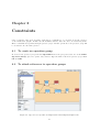
8 Constraints
8.1 To create an operation group . . . . . . . .
8.2 To attach references to operation groups . .
8.3 To constraint operation groups on operators
8.4 To delete an operation group . . . . . . . .
.
.
.
.
.
.
.
.
.
.
.
.
.
.
.
.
.
.
.
.
.
.
.
.
.
.
.
.
.
.
.
.
.
.
.
.
.
.
.
.
.
.
.
.
.
.
.
.
.
.
.
.
.
.
.
.
.
.
.
.
.
.
.
.
.
.
.
.
.
.
.
.
.
.
.
.
.
.
.
.
.
.
.
.
.
.
.
.
.
.
.
.
.
.
.
.
.
.
.
.
.
.
.
.
45
45
45
46
46
9 Adequation
9.1 Main algorithm and main architecture
9.2 Characterization . . . . . . . . . . . .
9.3 To launch the adequation . . . . . . .
9.4 Multi-periodic applications . . . . . .
9.5 Flattening . . . . . . . . . . . . . . . .
Hierarchy . . . . . . . . . . . .
Abstract references . . . . . . .
9.6 Schedule . . . . . . . . . . . . . . . . .
9.6.1 To display the schedule . . . .
9.6.2 The schedule window . . . . .
Operator . . . . . . . . . . . .
Medium . . . . . . . . . . . . .
Start and end dates . . . . . .
Scale . . . . . . . . . . . . . . .
Colors . . . . . . . . . . . . . .
Schedule position . . . . . . . .
Other options . . . . . . . . . .
.
.
.
.
.
.
.
.
.
.
.
.
.
.
.
.
.
.
.
.
.
.
.
.
.
.
.
.
.
.
.
.
.
.
.
.
.
.
.
.
.
.
.
.
.
.
.
.
.
.
.
.
.
.
.
.
.
.
.
.
.
.
.
.
.
.
.
.
.
.
.
.
.
.
.
.
.
.
.
.
.
.
.
.
.
.
.
.
.
.
.
.
.
.
.
.
.
.
.
.
.
.
.
.
.
.
.
.
.
.
.
.
.
.
.
.
.
.
.
.
.
.
.
.
.
.
.
.
.
.
.
.
.
.
.
.
.
.
.
.
.
.
.
.
.
.
.
.
.
.
.
.
.
.
.
.
.
.
.
.
.
.
.
.
.
.
.
.
.
.
.
.
.
.
.
.
.
.
.
.
.
.
.
.
.
.
.
.
.
.
.
.
.
.
.
.
.
.
.
.
.
.
.
.
.
.
.
.
.
.
.
.
.
.
.
.
.
.
.
.
.
.
.
.
.
.
.
.
.
.
.
.
.
.
.
.
.
.
.
.
.
.
.
.
.
.
.
.
.
.
.
.
.
.
.
.
.
.
.
.
.
.
.
.
.
.
.
.
.
.
.
.
.
.
.
.
.
.
.
.
.
.
.
.
.
.
.
.
.
.
.
.
.
.
.
.
.
.
.
.
.
.
.
.
.
.
.
.
.
.
.
.
.
.
.
.
.
.
.
.
.
.
.
.
.
.
.
.
.
.
.
.
.
.
.
.
.
.
.
.
.
.
.
.
.
.
.
.
.
.
.
.
.
.
.
.
.
.
.
.
.
.
.
.
.
.
.
.
.
.
.
.
.
.
.
.
.
.
.
.
.
.
.
.
.
.
.
.
.
.
.
.
.
.
.
.
.
.
.
.
.
.
.
.
.
.
.
.
.
.
.
.
.
.
.
.
.
.
.
.
.
.
.
.
.
.
.
.
.
.
.
.
.
.
.
.
.
.
.
.
.
.
.
.
.
.
.
.
.
.
.
.
.
.
.
.
.
.
.
.
.
.
.
.
.
.
.
.
.
.
.
.
.
.
.
.
.
.
.
.
.
.
.
.
.
.
.
.
.
.
.
.
.
.
.
.
.
.
.
.
.
.
.
.
.
.
.
.
.
.
.
.
.
.
.
.
47
47
47
47
47
48
48
48
48
48
48
48
49
49
49
49
49
49
10 Code generation
10.1 To generate the code . . . . . . . . . . . .
10.2 To view generated files . . . . . . . . . . .
10.3 Overview . . . . . . . . . . . . . . . . . .
10.4 To compile an executive . . . . . . . . . .
10.5 To load the compiled executive . . . . . .
10.6 To automate the compilation/load process
.
.
.
.
.
.
.
.
.
.
.
.
.
.
.
.
.
.
.
.
.
.
.
.
.
.
.
.
.
.
.
.
.
.
.
.
.
.
.
.
.
.
.
.
.
.
.
.
.
.
.
.
.
.
.
.
.
.
.
.
.
.
.
.
.
.
.
.
.
.
.
.
.
.
.
.
.
.
.
.
.
.
.
.
.
.
.
.
.
.
.
.
.
.
.
.
.
.
.
.
.
.
.
.
.
.
.
.
.
.
.
.
.
.
.
.
.
.
.
.
.
.
.
.
.
.
.
.
.
.
.
.
.
.
.
.
.
.
.
.
.
.
.
.
.
.
.
.
.
.
.
.
.
.
.
.
.
.
.
.
.
.
50
50
50
50
51
51
51
.
.
.
.
.
.
.
.
.
.
.
.
.
.
.
.
.
5
11 SynDEx downloader specification
11.1 Context . . . . . . . . . . . . . .
11.2 Boot and download process . . .
11.3 Common download format . . . .
11.4 Downloader macros . . . . . . . .
.
.
.
.
.
.
.
.
.
.
.
.
.
.
.
.
.
.
.
.
.
.
.
.
12 Links
.
.
.
.
.
.
.
.
.
.
.
.
.
.
.
.
.
.
.
.
.
.
.
.
.
.
.
.
.
.
.
.
.
.
.
.
.
.
.
.
.
.
.
.
.
.
.
.
.
.
.
.
.
.
.
.
.
.
.
.
.
.
.
.
.
.
.
.
.
.
.
.
.
.
.
.
.
.
.
.
.
.
.
.
.
.
.
.
.
.
.
.
.
.
.
.
.
.
.
.
.
.
.
.
53
53
53
54
54
56
6
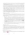
Introduction
This manual uses some writing conventions:
• menus, buttons etc. are written in bold
(e.g. File menu, OK button, Definition list, Launch Adequation option),
• SynDEx directories and files, examples etc. are written in Computer Modern
(e.g. libs directory, examples/tutorial/example7/example7 sdc.sdx file, ! int o port definition),
• notions, windows, etc. are written in italic:
(e.g. AAA methodology, reference, definition mode, algorithm window ).
7
Chapter 1
Overview
1.1
The AAA methodology
SynDEx is based on the AAA methodology (cf. chapter 12).
A SynDEx application is made of:
• algorithm graphs (definitions of operations that the application may execute),
• architecture graphs (definitions of multicomponents: set of interconnected processors and specific
integrated circuits).
Performing an adequation means to execute heuristics, seeking for an optimized implementation of a
given algorithm onto a given architecture.
An implementation consists in:
• distributing the algorithm onto the architecture (allocate parts of algorithm onto components),
• scheduling the algorithm onto the architecture (give a total order for the operations distributed
onto a component).
1.2
SynDEx distributions
SynDEx runs under Linux, Windows, and Mac OS X platforms. SynDEx is written in Objective Caml.
The Graphical User Interface is written in Tcl/Tk with the OCaml library CamlTk. See chapter 12 for
web links.
8
Chapter 2
Getting started
2.1
2.1.1
Application workspace
Launching SynDEx
SynDEx is launched by running the SynDEx executable, located in the directory bin of your installation
directory. Some options can be specified on the command line, for example :
• -libs adds a directory where to find libraries to include (see chapter 3),
• -html specifies the path of the internet browser that displays the manual and tutorial html documentations from the Help menu. The url to open is appended at the end of the specified command.
You can also try to use %s in the specifed command to make SynDEx replace this %s by the url in
the command. In this case do not forget to put the command between “ ” .
The complete list of options can be obtained by running the SynDEx executable with the --help
option.
For example write the command line:
> /syndex-7.0.x/bin/syndex-7.0.x -libs /syndex-7.0.x/libs -html /usr/bin/firefox appli.sdx
In this example the libraries directory and the web browser used to display the manuals are specified
on the command line. In addition, the name of an application to open is also specified, otherwise only
the principal window is opened.
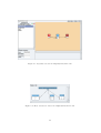
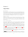
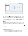
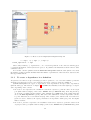
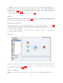
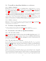
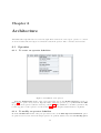
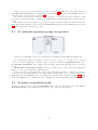
2.1.2
SynDEx principal window
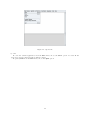
To create an application workspace, run the SynDEx executable without the name of an application. It
opens the principal window of SynDEx (cf. figure 2.1).
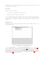
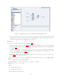
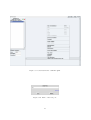
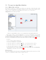
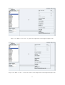
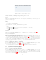
2.1.3
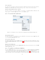
Load a SynDEx application
To load an existing application in the workspace, from the File menu, choose the Open option and select
a SynDEx file (cf. figure 2.2). For example load the /syndex-7.0.x/examples/basic/basic.sdx example.
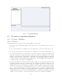
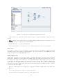
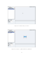
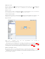
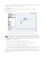
2.1.4
Algorithm and architecture windows
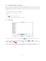
Loading a SynDEx application will open:
• the algorithm window on the main algorithm if it have been defined (cf. figure 2.3),
• the main architecture window if the main architecture have been defined (cf. figure 2.4).
9
Figure 2.1: SynDEx principal window
Opening another application will replace the current one by the new one in the workspace.
Warning: some application may require libraries (cf. Chapter 3).
2.2
Modes
In the algorithm window, the adress bar displays AlgorithmMain (main) meaning that the main algorithm
is viewed in the main mode (cf. section 5.1.2). Double left click on AlgorithmMain in the Definition list.
The algorithm is now viewed in its definition mode and the adress bar displays [Function] AlgorithmMain.
See section 5.1.2 for more information.
Note that you can create several algorithms and architectures but only one main algorithm and one
main architecture on which the adequation will be applied.
2.3
Adequation and code generation
To launch the adequation of the main algorithm (cf. Main mode in section 5.1.2) onto the main architecture (cf. section 6.3.2), from the Adequation menu of the principal window, choose the Launch
Adequation option. To save the result of the adequation, from the Options menu, check Save Adequation with Application. Then save your application. To view the computed schedule, from the
Adequation menu, choose the Display Schedule option. See chapter 9 for more information.
To generate the code of the application, from the Code menu, choose the Generate Executive(s)
option. The generated .m4 files are saved in the example’s directory. To view theses files from the
SynDEx workspace, from the Code menu, choose the Display Executive(s) option. See chapter 10
for more information.
2.4
Save, Close, Quit
To save the current application, from the File menu, choose the Save option. To save it with a new
name, choose the Save as option and type the new name in the dialog window. The file will be suffixed
10
Figure 2.2: Open a file
by .sdx.
To close the current application, from the File menu, choose the Close option. It closes all the
application windows and leaves the workspace empty.
To quit SynDEx from the File menu, choose the Quit option.
11
Figure 2.3: Algorithm window in examples/basic/basic.sdx
Figure 2.4: Main architecture window in examples/basic/basic.sdx
12
Chapter 3
Libraries
3.1
To use libraries
To create a new application you may want to use pre-defined algorithm or architecture definitions contained in libraries. These definitions are called global definitions (vs. local definitions from the current
application).
From the File menu of the principal window, choose the Specify Library Directories option. Then
left click on the Add button of the dialog window and select the target directory. For example, specify
the SynDEx libs directory and the examples/basic with library/basicLibraries directory.
To include a library in an application in order to make references to the objects it contains, from
the File menu of the principal window, choose the Included Libraries option. Then check the target
library. Uncheck an already included library to un-include it, provided there are no references in your
application on definitions from this library.
3.2
To create a library
To create a library of algorithm or architecture definitions, you must create a .sdx file containing the
definitions you need. Libraries may be located in the libs directory, at the root of your installation
directory. Or you will have to specify their location to the SynDEx application (cf. section 3.1).
13
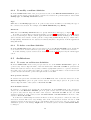
Chapter 4
Using the interface
4.1
Selection
Selection may be applied to vertices or edges of both algorithm or architecture graphs.
Left click on a vertex (resp. an edge). Red squares appear on its borders, meaning that the vertex
(resp. the edge) is selected. To select multiple vertices and/or edges, use the shift key. To select a set
of vertices and/or edges, use the left button of the mouse while dragging it, in order to draw a square
when the button is released. Vertices inside or intersecting the square are selected.
To move a selection, left click on a vertex of the selection. Then drag it until the target position and
release the mouse. To cancel a selection left click outside the selection.
Contextuals menus are available on selections (cf. section 4.3).
4.2
Zoom
Zoom may be applied to architecture (cf. chapter 6) and schedule windows (cf. section 9.6) by moving
the zoom cursor on the border of these windows.
4.3
Contextual menus
Some contextual menus are available in SynDEx. Contextual menus mainly include edition commands
(Copy, Cut, Paste, Delete).
Algorithm window
In the algorithm window, right click on the background of an algorithm definition window. It opens
a contextual menu on the target definition. Left click on a vertex (function, delay, sensor, actuator,
constant ) of an algorithm graph. Red squares appear. Then right click the mouse. It opens a contextual
menu on the target reference.
The Activate Info Bubbles option displays additionnal information when pointing the cursor at a
vertex of any algorithm graph.
Architecture window
In an architecture window, right click on the background or left click on the Edit menu. It opens a
contextual menu on the target definition. Left click on a vertex (operator, communication medium) of
an architecture graph. Red squares appear. Then right click the mouse. It opens a contextual menu on
the target reference.
14
4.4
Contextual information
When the cursor points at an object of an algorithm (cf. chapter 5), an architecture (cf. chapter 6) or
a schedule window (cf. section 9.6), information is displayed in the principal window.
By default information is not kept when switching between objects. The new information overwrites
the older one. To change this behaviour and keep all the information, from the Options menu of the
principal window, check Keep Information in the Principal Window. This is for instance useful
when the information displayed does not fit in the window, which requires to scroll the principal window.
4.5
To find an object
Looking for a vertex, from which you now the name, in a complex graph can become rather tedious.
Architecture window
In the architecture window (cf. chapter 6), from the Edit menu, choose the Find Operator Reference
or Find Medium Reference option to locate a vertex of your graph by its name. It opens a window
listing all the vertices of your graph. Double left clicking on one of them will select it.
Schedule window
In the schedule window (cf. section 9.6), from the Edit menu, choose the Find Operation option to
locate an operation of your graph by its name. It opens a window listing all the operations of your graph.
Double left clicking on one of them will select it.
4.6
Refresh
To refresh an architecture window, from its Window menu, choose the Refresh option. If necessary,
re-open the algorithm window (cf. Algorithm window in chapter 5) to refresh it.
15
Chapter 5
Algorithm
AAA methodology
In the AAA methodology, an algorithm is specified as a directed acyclic graph (DAG) infinitely repeated.
Directed means that for each edge representing a relation between vertices, the vertices tuple is ordered,
i.e. its first element is the source vertex and the other one(s) is(are) the destination vertex(vertices). A
vertex is an operation corresponding to a sequence of instructions which starts after all its input data are
available and produces all its output data at the end of the sequence. An edge is a dependence between
two vertices corresponding to a data transfer and an execution precedence, or to an execution precedence
only. Note that some vertices may be independent, i.e. may not be connected by dependences.
Definition vs. reference
In SynDEx there is a distinction between algorithm definition and algorithm reference. A definition
preexists to a reference that corresponds to one an only one definition. On the contrary, to a given
definition may correspond several references. That allows for referencing, with different names, a unique
definition. Therefore, an algorithm is described by a definition, which is a DAG similar to those in
AAA, where vertices are references or ports, and edges are dependences between references, or between
references and ports.
Atomic or hierarchical definitions
To a given reference contained in a definition corresponds a definition which may contain itself several
references, and so on. That corresponds to hierarchy. A definition is said hierarchical when it defines
an algorithm which contains at least one dependence connecting an input port to an output port, and
possibly one or several references connected by dependences, otherwise it is said atomic.
There are five types of atomic definitions: functions read data on input ports, execute instructions
without any side-effect, write data on output ports, sensors are input vertices of the DAG producing
data from a physical sensor, actuators are output vertices of the DAG consuming data for a physical
actuator, constants are input vertices of the DAG, with null execution time, delays memorize data
during one or several infinite repetition of the DAG, for use in next repetitions. These types are detailed
in section 5.1.1.
A definition is said explicitly hierarchical when the algorithm contains at least one dependence (and
possibly references). This includes conditioning (cf. section 5.2), repetitions (cf. section 5.3) of hierarchical definitions, and more generally definitions defined through several levels of hierarchy. Only a
function may be defined through explicit hierarchy.
A definition is said implicitly hierarchical when the algorithm does not contain any dependence and
yet will be transformed by SynDEx, for the adequation, into a graph which contains dependences. This
happens only with repetitions (cf. section 5.3) of atomic definitions.
Warning: A hierarchical definition does not have to wait for all its input data to be available before
starting some computations. Indeed, parts of the algorithm graph of a hierarchical algorithm definition
may only require parts of the input data of the definition and therefore can start as soon as this part
16
is available (and not all the data). In the same way, some data may be produced before the end of the
complete sequence of computations.
Dependences
There are two types of dependences:
• data dependence: data transfer and execution precedence,
• precedence dependence: execution precedence only.
A data dependence imposes that the reference at the source of the dependence, produces data and
is executed before the reference at the destination of the dependence, which consumes the data. A
precedence dependence only imposes an execution order between references, no data is produced or
consumed.
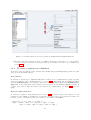
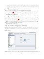
Algorithm window
Definitions and references are managed through analgorithm window. If necessary it is possible to open
several algorithm windows.
Figure 5.1: Algorithm / New Algorithm Window
From the Algorithm menu, choose the New Algorithm Window option (cf. figure 5.1). It
opens an algorithm window for algorithm definitions (cf. figure 5.2). Left click on the background of a
definition window : the algorithm window shows its Definition Properties. Left click on a reference
in this definition window : the algorithm window shows its Reference Properties. These definition or
reference properties appear in the left bottom part of the algorithm window (cf. figure 5.4 for definition
properties and figure 5.5 for reference properties).
17
Figure 5.2: Algorithm Window
5.1
5.1.1
To create an algorithm definition
To create a definition
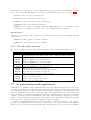
Types of definitions
SynDEx distinguishes five types of definitions with different edition rules:
• a function is a general abstraction with no edition restriction: it can contain dependences, references
and ports;
• a sensor is an abstraction of a physical device producing data: it can only contain output ports;
• an actuator is an abstraction of a physical device consuming data: it can only contain input ports;
• a constant is a an abstraction of a typed value: it can only contain one output port producing that
value. For convenience, the value hold by the constant can be given as a parameter to the constant
definition. Note that this is only possible for values that are representable within the parameter
language: integer, float, string and list of such values. SynDEx standard library uses this trick
to define constants for the library base types (int, float, ...). For example, the cst definition of
the int library has one parameter: ListOfValues;
• a delay is an abstraction of a memory region: it must contain one input port (the write port) and
one output port (the read port) of the same type, but nothing more. Delays hold the state of a
SynDEx application. Using delays is the only way to propagate data from one iteration of the
application to the next. A delay must be initialized, either by using a parameter (as suggested
above for constant definitions) or lately in the real world code (as for constant definitions, doing it
in the code is the only alternative for delays holding values of complex types). SynDEx standard
library defines delays for its base types as shift registers with two parameters: the first one is a list
of initial values and the second one is the size (in number of elements) of the shift register. For
example, the delay definition of the int library has two parameters: listInit and nbDelay.
18
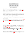
Figure 5.3: Definition of a sensor
New definition
To create a new definition, in the algorithm window, left click on the + green button. It opens a dialog
window in which you can select the definition’s type. For example check Sensor (cf. figure 5.3). Type
the name of the new sensor and optionally parameters. For example type input. Then left click OK.
It creates a definition of sensor named input.
Definition with parameters
Parameters are local to the scope of a definition. Often, parameters are used to create more generic
definitions. For example, the increment of an incrementer can be given as a parameter of the incrementer
definition. Parameters of a definition are names (not values) separated by semi-colon between < and >
following the name of the definition, according to the following syntax:
parameters ::= "<" { parameter ";" } parameter ">"
parameter ::= name
where curly brackets {...} represent zero, one or several repetitions of the enclosed element, and
keywords are quoted.
You can also edit the parameters of a definition directly in its Definition Properties (cf. figure 5.8)
using the same syntax. The parameters will be instanciated (values given to names) when the definition
will be referenced (cf. section 5.1.4). The only definition whose parameters can be instanciated, is the
main algorithm (cf. section 5.1.2) only through its field Values in its Definition Properties (cf. figure
5.8).
5.1.2
Definition mode and main mode
This section refers to section 2.2.
Definition mode
Double left click on a definition name in the Definition list (e.g. open the examples/hierarchy/hierarchy.sdx
application and double left click on C in the Definition list). You are now in a definition mode (cf.
figure 5.4). From a definition mode, to open the definition corresponding to a reference in order to inspect and possibly modify its content, left click on the target reference to select it. Red squares appear
on its borders (cf. figure 5.5). Then double left click on it. It displays the definition of the target
reference (cf. figure 5.6).
Note that as soon as you have included an algorithm library (cf. section 3.1), all its definitions
appear in the definition list. The Definition list in figure 5.4 shows some local definitions (e.g.
A,
B, C, Main) and global definitions (e.g. int/Arit add, int/Arit div, etc.) since the integer library
was included.
Main mode
To define an algorithm as main, right click on the background of the target definition window. Choose
the Set As Main Definition option (cf. figure 5.7). The color of the background changes and the
19
Figure 5.4: C definition in examples/hierarchy/hierarchy.sdx
adress is changed from a [Function] to a (main), meaning that you are now in the main mode on the
main algorithm (cf. figure 5.8). Note that the main algorithm must be at the root level of a hierarchy;
it can not contain unconnected ports. Only the main algorithm can instanciate (give values to names)
its parameters (cf. section 5.1.1) thanks to its field Values in its Definition Properties (cf. figure 5.8).
Left click on the Main button of the algorithm window. It displays the main algorithm in the main
mode. Left click on a hierarchical reference to browse down the main algorithm (e.g. left click on the
C reference of Main then left click on the B2 reference of C). Then left click on Up In Main to browse
up the main algorithm.
Hierarchy
Now you may construct a graph with references to constants, sensors, actuators, delays and functions.
If this definition is intended to be referenced in an explicit hierarchy, i.e. this reference will belong to
a certain level of hierarchy (possibly a leaf), you must use input and output ports. If this definition
is intended to be referenced at the root level of the hierarchy, input ports are replaced by sensors and
output ports are replaced by actuators.
References to an explicitly hierarchical definition are displayed with a double-border (in the figure 5.4
B1 is a reference on an explicitly hierarchical definition contrary to add).
5.1.3
To create a port in a definition
Ports are communication interface of a definition with the outside world.
Direction of ports
SynDEx distinguishes three directions for ports:
• an input port represents a data that is provided by the outside world to the definition;
• an output port represents a data that is provided by the definition to the outside world;
20
Figure 5.5: Opening B1 reference in examples/hierarchy/hierarchy.sdx
• an input/output port can be seen as a reference (or pointer) to a data provided by the outside
world that the definition can modify in place. This explains the name of input/output ports: we
can read the value of the port and replace it by a new one.
New port
To create a port in an atomic definition (cf. chapter 5):
• in the definition mode (cf. section 5.1.2), right click on the background and choose the Create
port option For example create a new definition named input and create a port in this definition
(cf. figure 5.9);
• it opens a dialog window in which you can type the port direction, type, name and optionally its
size. You can left click on the syntax help link for more information. For example type ! int
o, then left click OK (cf. figure 5.10);
• it creates the target port. In this example, the new port is an integer output port named o (cf.
figure 5.11) in the definition window.
You can undo and redo this action, right click on the background and choose the Undo, Redo
options.
A port definition has the following syntax:
port_definition ::= direction type [ "[" size "]" ] name
direction ::= "?" | "!" | "&"
where:
• ? specifies an input port,
• ! specifies an output port,
• & specifies an input/output port,
21
Figure 5.6: B definition in examples/hierarchy/hierarchy.sdx
square brackets [...] represent optional elements, pipes | represent alternatives, and keywords are
quoted.
Hint: you can create several ports in one breath by simply putting several port definitions in a row
in the dialog window, according to the following syntax:
port_definition ::= { port_definition }
where curly brackets {...} represent zero, one or several repetitions of the enclosed element.
Ports order
If you plan to generate code, it is necessary to specify an order for ports which is consistent with the
declaration of the corresponding executable function. To specify the ports order, right click on the
background and choose the Ports Order option.
Input/output ports
Input-output ports have a very specific behavior concerning data memory allocation in the executives
generated by SynDEx. For any application, SynDEx makes data buffer allocations for (and only for)
the output ports of the atomic references of your algorithm graph. Input-output ports do not cause
an allocation but instead an alias on the output port of its predecessor. The operation containing this
input-output port directly modifies the value of its predecessor port (side-effect). This is useful to avoid
reallocation of big data buffers of the same type (for instances images) by making successive computations on the same data buffer.
However, as side-effects are not supposed to happen in data-flow graphs, this comes with some
restrictions:
• Ports of delay definitions can not be input/output ports,
• Ports of hierarchical definitions can not be input/output ports,
22
Figure 5.7: Set Main definition as main algorithm in examples/hierarchy/hierarchy.sdx
• The data of an input/output port can not be diffused: if there is a dependence A.o --> B.io (where
A.o is an output port and B.io is an input/output port), neither A.o nor B.io can be diffused (cf.
section 5.3.1).
5.1.4
To create a reference in a definition
A reference can be thought as a call to a function in a traditional programming language. Here the called
function is an algorithm definition.
New reference
To reference a definition (e.g. myReferencedDef) into another one (e.g. myDefinition), set the algorithm
window in definition mode on myDefinition (cf. section 5.1.2). Then drag and drop myReferencedDef
from the Definition list to the definition window (or select myReferencedDef in the Definition list,
right click on the background of the definition window, and choose the Create reference option). It
opens a dialog window. Type the name of the reference (e.g. myReference). See figure 5.12 to see the
result.
Reference with parameters
To reference a definition with parameters (cf. section 5.1.1), a valued expression is required for each
parameter of the definition. Parameters of a reference are valued expressions separated by semi-colon
between < and > following the name of the reference, according to the syntax:
expr_list ::= "<" { expr ";" } expr ">"
expr ::= name | value | "(" expr ")" | expr "+" expr |
expr "-" expr | expr "*" expr | expr "/" expr |
23
Figure 5.8: Main mode in examples/hierarchy/hierarchy.sdx
"-" expr | "{" { expr "," } expr "}"
valued_expression ::= expr
where curly brackets {...} represent zero, one or several repetitions of the enclosed element, pipes
| represent alternatives, and keywords are quoted. A parameter is instanciated when it has a value
otherwise it is not.
You can also edit the parameters in the Reference Properties with the same syntax. Note that
the number of valued expressions must match the number of parameters of the referenced definition, and
that types must match.
5.1.5
To create a dependence in a definition
A dependence is a directed edge connecting a producer operation to one or several consumer operations.
As such, it specifies an execution order relation between two references used in a definition.
SynDEx distinguishes two types of dependences: data dependences and precedence dependences
(without data) (cf. introduction of chapter 5). SynDEx automatically creates the right type of dependence depending on the context:
• To create a data dependence in a definition between two references, point the cursor at an output
port (little black rectangle) of the source, middle click (or Ctrl left click), then drag and drop
on an input port (little black rectangle) of the destination (or right click on the background, and
choose the Add dependence option). The source and destination of a data dependence can also
be ports: this is used to read a data from (resp. write a data to) the outside world. Note that for a
given non-atomic definition, all output ports must be in dependence with input ports: all outputs
must be defined;
• To create a precedence dependence in a definition between two references, point the cursor at an
output precedence port (little black rectangle) of the source, middle click (or Ctrl left click), then
24
Figure 5.9: Contextual menu → Create port
Figure 5.10: Name of the new port
25
Figure 5.11: A definition after port creation
Figure 5.12: A reference to myReferencedDef into myDefinition
26
drag and drop on an input precedence port (little black rectangle) of the destination. Input (resp.
output ) precedence ports are represented by little black squares at the left (resp.right) of the boxes
holding the reference names.
5.1.6
To create a superblock
A superblock is a set of operations, edges and ports extracted as a new definition.
To create a definition as a superblock, select the target set of operations, edges and ports you want
to extract (cf. section 4.1). Then right click and choose the Extract as superblock option. A new
definition is created and a reference to this definition replaces the selected set. The new definition is
available in the Definition list, You can rename both the definition and the reference.
You can undo and redo this action.
5.1.7
To create an abstract reference
An abstract reference is a reference to a hierarchical definition in which the hierarchy is not taken into
account, i.e. the flattening (cf. section 9.5) does not go into the hierarchical referenced definition that
becomes therefore abstract. However, note that to perform the adequation this definition must have a
duration.
To create an abstract reference, select the desired hierarchical reference then, check the option Abstract in the Reference properties of this reference.
You can undo and redo this action.
5.2
To condition an algorithm definition
First make sure that the target definition contains an input port of type int for the conditioning port.
Note that the SynDEx libs directory already provides an int library for operations on integer values.
New condition
Figure 5.13: switch definition mode for cond = 3 in examples/condition/simpleCondition/simpleCondition.sdx
27
Right click on the background of the definition window and choose the Create Condition option.
It opens a dialog window for the new condition. A condition is a port = value expression where port is
the name of the conditioning port and value is an integer. Note that the conditioning port must be of
direction input (cf. 5.1.3). A new tab is created for the given condition. The conditioning port is now
colored in yellow (cf. figure 5.13).
If necessary, refresh the algorithm window (cf. section 4.6).
Remarks
Note that there can be only one conditioning input port. You have to construct one sub-graph per value
associated to a conditioning input port (cf. figure 5.13). For each other value of the conditioning input
port, the result is unspecified and will be inconsistent.
CondI and CondO vertices
The adequation and the code generation will take into account the expanded graph (cf. section 9.5).
SynDEx will introduce new vertices during the expansion: CondI and CondO vertices.
A CondI vertex consumes the conditioning data and connects the input ports of the conditioned
operation according to its value.
A CondO vertex consumes the conditioning data and connects the output ports of the conditioned
operation according to its value.
References
Figure 5.14: conditioned definition mode in examples/condition/simpleCondition/simpleCondition.sdx
In a definition mode (cf. section 5.1.2), references to conditioned definitions have their conditioning
port yellow colored (cf. figure 5.14).
Delete a condition
Right click on the background of the definition window and choose the Delete Condition option.
28
5.3
5.3.1
To repeat an algorithm definition
Diffuse, Fork, and Join
You can create a reference to a definition, and connect to its input (resp. output ) ports some output
(resp. input ) ports with different sizes. The pre-condition is to have a unique common multiple between
each pair of ports of different sizes. This multiple is the repetition factor of the reference.
Multiplication of a vector by a scalar
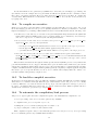
Figure 5.15: AlgorithmMain1 definition mode in examples/tutorial/example4/example4.sdx
Suppose that you want to specify the multiplication of a vector by a scalar giving a vector as result
(cf. AlgorithmMain1 in examples/tutorial/example4). You can specify it by repeating the multiplication
between two scalars instead of defining a new one. For example for N length vectors, you may specify
the repetition by N multiplications between scalars giving a scalar as a result (cf. figure 5.15).
You have to:
• create a definition with the parameter N,
• reference the multiplication on scalars mul,
• connect the output port of a scalar (e.g. s input) to one of its input ports (e.g. mul.a),
• connect the output port of a vector (e.g. v input) to the other input port (e.g. mul.b),
• connect its output port (mul.o) to the input port of a vector (e.g. v output),
• set the repetition factor of mul to N: left click on the mul reference, then type N in its Reference
Properties (cf. Algorithm window in chapter 5).
Repetition factor
The common multiple between each pair of ports with different sizes is N. It is the repetition factor that
you have to set explicitely by using a symbolic numbered expression.
29
Diffuse the scalar
Since the output port of s input has the same size as its connected input port of the multiplication
function, it is replicated N times in order to be multiplicated by each element of v input. This is a
Diffuse operation.
Fork the vector
Since the function operates on scalars and the v input vector has N elements, each of its elements are
provided separately in order to be multiplicated. This is a Fork operation.
Join the internal results
Since the function operates on scalars and the v output vector has N elements, each repetition of the
multiplication is taken in order to be provided as a N elements vector. This is a Join operation.
Representation
Figure
5.16:
matprodvec
main
examples/tutorial/example4/example4.sdx
mode
from
AlgorithmMain3
main
algorithm
in
The repetition factor is displayed next to the name of the reference (e.g. in the figure 5.15 mul is
repeated N times). The main algorithm (e.g. AlgorithmMain3) instanciates its parameters (cf. figure 5.8).
From the main mode in examples/tutorial/example4/example4.sdx (cf. section 5.1.2), double left click
on the matprodvec reference, the dotprod reference is repeated three times (cf. figure 5.16).
Explode and Implode vertices
The adequation and the code generation will take into account the expanded graph (cf. section 9.5).
SynDEx will introduce new vertices during the expansion: Explode and Implode vertices.
An Explode vertex extracts for each repetition of a definition each element of the data it receives (cf.
subsections Diffuse and Fork ).
30
An Implode vertex builds the data it sends by concatenating each separated element produced by
each repetition of the definition (cf. subsection Join).
5.3.2
Iterate
In some cases, you may want to repeat a reference but have no difference between port sizes.
Multiplication of two vectors
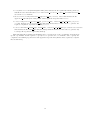
Figure 5.17: dp definition mode in examples/tutorial/example4/example4.sdx
Suppose that you want to specify the multiplication of two vectors giving a scalar as a result (cf. figure
5.17). You can specify it by repeating the multiplication between two scalars, that used an accumulator
to store the partial sum. For example if for dpaccn length vectors, you may specify the repetition by
dpaccn multiplications between three scalars (the i element of the first vector, the i element of the second
one, and the accumulator, initialized to 0).
You have to:
• reference the multiplication on scalars with accumulator (e.g. dp),
• connect two vectors (e.g. v1 and v2) to the scalar input ports of the multiplication,
• connect a {0} constant to the acc input port of the multiplication,
• connect the output port of the multiplication to a scalar (e.g. dp),
• connect the acc output port of the multiplication to its acc input port choosing an Iterate edge,
• repeat dpaccn times the multiplication (in the Reference Properties of the dpacc reference).
The accumulator is initialized with {0}. Then the output of the repetition i becomes the accumulator
of the repetition i+1. The output of the last repetition is the output of the repeated definition. This is
an Iterate operation.
31
5.4
5.4.1
To modify an algorithm definition or a reference
Modify a definition
Double left click on the definition name in the Definition List or double left click on a reference
from a definition mode (cf. section 5.1.2). It opens its definition window. Right click on the background
of the definition window. Choose the Create dependence option (cf. section 5.1.5), Create port (cf.
section 5.1.3), Create reference (cf. section 5.1.4), Create Condition or Delete Condition (cf.
section 5.2) to modify the definition.
As soon as you have Left clicked on the background of a definition window (cf. Algorithm window in
chapter 5) you can change its Definition Properties to modify its Name, Description, Parameters
or Values. The latter property appears only in the case of a main algorithm definition.
Note that you can modify local and global definitions (cf. section 3.1). Modifications on a global
definition impact only the current application and the library remains unchanged. To modify a global
definition over-all, open the corresponding SynDEx library file (e.g. libs/int.sdx). Modifications on a
definition in a library may have consequences on all the applications using this library.
5.4.2
Modify a reference
Left click on a reference in a definition window (cf. Algorithm window in chapter 5). Use its Reference
Properties to modify its Name, Parameters, Repeat or Period. For the period see the section 5.7
“To build mutli-periodic applications”.
5.5
To delete an algorithm definition
To delete a definition, in the algorithm window, left click on the - red button.
Note that deleting a global definition (cf. section 3.1) impacts only the current application.
5.6
5.6.1
To associate code with an algorithm definition
The code editor window
Right click on the background of a definition window. Choose the Edit code phases option (cf. figure
5.18). Check init (resp. end) to generate code in the initialization phase (resp. ending phase).
Right click on the background of a definition window. Choose the Edition of the associated
source code option (cf. figure 5.19). It opens the code editor window on the initialization phase for the
selected definition. Left click on loop phase (resp. end phase) to edit the code associated in the loop
phase (resp. ending phase) (cf. figure 5.20).
5.6.2
The code editor macro language
From the Code menu of the principal window, check Generate m4x files. At code generation
time, the code written in the code editor will be wrapped into M4 macro code, and outputed into
an application name sdc.m4x file. These files contain one M4 macro definition per algorithm definition
(cf. figure 5.21). The code editor offers several macros to abstract away the M4 nature of the output
file. These macros are of two kinds: port and parameter names translation macros, and quoting macros
(cf. macros directory).
Names translation macros
Parameter and port names of an algorithm definition are encoded as parameters of the corresponding
M4 macro. Because the M4 language uses positional parameters, when you want to refer to a parameter
or port in the associated code he has to know its position in the M4 macro parameters list. More than
being not very handy, this is fragile relatively to creation or deletion of ports and parameters in the
definition: when you create a port or a parameter to a definition, he has to adjust (replace $n by $n+1
32
Figure 5.18: Edition of the conv code phases in examples/tutorial/example7/example7.sdx
Figure 5.19: Edition of the code associated with conv in examples/tutorial/example7/example7.sdx
33
Figure 5.20: Code associated with conv in loop phase in examples/tutorial/example7/example7.sdx
Figure 5.21: M4 macro code for conv in examples/tutorial/example7/example7 sdc.sdx
34
in) all references to parameters or ports coming after the created one in the parameters list of the M4
macro. To overcome this difficulty, the code editor recognizes the following macros (cf. figure 5.20):
• @IN(prt) refers to the input port named prt,
• @OUT(prt) refers to the output port named prt,
• @INOUT(prt) refers to the input/output port named prt,
• @PARAM(prm) refers to the parameter named prm,
• @NAME(pr) refers to the port or parameter named pr. When using this macro, you should be careful
that the port or parameter you want to refer to has a unique name in the definition.
Quoting macros
Quoting macros are used to wrap or unwrap code by M4 quote. The code editor recognizes the following
quoting macros:
• @QUOTE(txt) will be put as ‘txt’ in the output file,
• @TEXT(‘txt’) will be put as txt in the output file.
5.6.3
The code editor shortcuts
The code editor supports various keyboard shortcuts that could be handy when editing source code.
Ctr-Tab
Tab
Ctr-I
Ctr-O
Ctr-N
Ctr-P
Ctr-T
Ctr-Q
Ctr-W
Ctr-K
Alt-W
Ctr-Y
Ctr-A
Ctr-E
Ctr-up
Ctr-down
5.7
Insert a tabulation.
Complete a port name. Type the beginning of a port name, then press Tab
and as many times as necessary for the editor to find the wanted completion.
Insert the @IN macro at cursor position.
Insert the @OUT macro at cursor position.
Insert the @INOUT macro at cursor position.
Insert the @PARAM macro at cursor position.
Insert the @TEXT macro at cursor position.
Insert the @QUOTE macro at cursor position.
Cut the selected text into the clipboard.
Cut text from cursor position to the end of the line.
Copy the selected text into the clipboard.
Paste the clipboard content at cursor position.
Jump to the beginning of the line.
Jump to the end of the line.
Jump to the beginning of the buffer.
Jump to the end of the buffer.
To build multi-periodic applications
Until version 6 of SynDEx a unique timing information (execution duration) is associated to each operation (resp. each data type of a dependence) relatively to the operators (resp. media) it may be distributed
onto. This timing information, which depends on the hardware, is associated to the definition of every
operation. Applications specified by the user with version 6 are implicitely mono-periodic, meaning that
all the operations of the algorithm graph have the same period which is equal to the total execution time
of all the operations executed on the different components of the architecture, taking into account the
duration of data communications through the media. This total execution time is displayed as the value
of the “Cycle time” in the schedule window resulting from the adequation.
Version 7 of SynDEx allows the user to specify, in addition to a duration, a period to each operation.
The period is a timing information associated to the reference of an operation instead of its definition,
which does not depend on the hardware. This feature allows the user to specify an operation definition
35
with the same execution duration each time it is referenced, whereas this operation may be referenced
with several periods. Note that for a given operation it is necessary that its execution duration is
smaller than its period to be schedulable.
As soon as a period is associated to an operation reference, the application becomes multi-periodic,
and a period must be associated to every operation reference. If it is not the case the application remains
mono-periodic. For both mono-periodic and multi-periodic applications, execution durations must be
associated to operation definitions and data type of dependences. A multi-periodic application has a
hyper period equal to the LCM (Least Common Multiple) of all the periods associated to the operation
references. This hyper period is displayed as the value of the “Cycle time” in the schedule window
resulting from the adequation. Note that the “Cycle time” is different from the total execution time
of all the operations executed on the different components of the architecture, taking into account the
duration of data communications through the media.
Version 7 of SynDEx, using the period and the execution duration of every operation, performs a
distributed real-time schedulability analysis. If the application is schedulable, SynDEx may generate the
corresponding macro-code (or may not find any schedule).
Version 7 of SynDEx, using the period and the execution duration of every operation, performs a
distributed real-time schedulability analysis to determine if the multi-periodic application is schedulable.
If it is the case it will generate the corresponding macro-code.
Multiple or equal periods
Operations related by a dependence must have multiple or equal periods. While creating a dependence between operations which have inconsistent periods, an error message appears to help the
user (e.g. Can not create dependence input.o -> compute.in in definition basicAlgorithm Error #1
[Inconsistent periods]).
While creating a dependence between operations which have multiple periods, there are two cases:
• the producer operation has a period p smaller than the period n of the consumer operation. In
this case the producer operation executes n/p times more than the consumer operation and consequently, produces n/p data for the consumer operation involving that these data are memorized. SynDEx displays a warning message indicating that the destination port’s size will be increased (e.g. #1 Warning about dependence input.o -> compute.in in definition basicAlgorithm
[The size of destination compute.in will increase to 2 times the original size]). In addition,
it creates a new operation called with the data type of the dependence prefixed by “Implode ” (e.g.
Implode int). This new operation is in charge of collecting the n/p data for the consumer operation. Note that the user must give a duration to this new operation. In case he forgot it a warning
message will ask for during the adequation ;
• the producer operation has a period p greater than the period n of the consumer operation. In
this case the consumer operation executes p/n times more than the producer operation and consequently, the consumer operation consumes p/n times the same data.
Hierarchical references
Verifications on periods are propagated to hierarchical references.
While setting the period to a hierarchical reference, SynDEx verifies that the new period is compatible
with the periods of the references it contains. Actually, the period of a hierarchical reference must be
equal (or multiple) to the Least Common Multiple (LCM) to the periods of the references it contains.
While setting the period to a reference contained in a hierarchical reference, SynDEx verifies that
the new period is compatible with the period of the hierarchical reference. Actually, the period of a
reference contained in a hierarchical reference must be equal (or must be a divisor) to the period of the
hierarchical reference.
Edit the period of an operation
The user can edit the period of an operation only in its reference properties (cf. paragraph “Algorithm
window ” in section 5) unlike its name, its parameters and its repeat factor which can also be edited
during the reference creation.
36
By default the period of an operation is equal to 0. Note that, as soon as an operation has a period
equal to 0, the application is mono-periodic whatever the other periods are. In other words, to obtain a
multi-periodic application the period of all the references must be edited.
Adequation
See the section 9.4 for details about the adequation process in case of mutli-periodic applications.
37
Chapter 6
Architecture
An architecture is specified as a non directed graph where vertices are of two types: operator or communication medium, and each edge is a connection between an operator and a communication medium.
6.1
6.1.1
Operator
To create an operator definition
Figure 6.1: Definition of an operator
From the Architecture menu of the principal window, choose the Define Operator option (cf.
figure 6.1). It opens a dialog window. Type the name of the new operator (e.g. U). Then left click OK.
It opens the new operator definition window (cf. figure 6.2). By default the code will be generated only
for the loop phase of the operator. See the section 6.1.2 to set its gates, durations and code phases.
6.1.2
To modify an operator definition
From the Architecture menu of the principal window, Choose the Edit Operator Definition option.
It opens a browse window. Select the target operator. It opens its definition window with Modify gates,
38
Figure 6.2: New U operator definition window
Modify durations, and Modify code generation phases buttons.
Gates
Left click on the Modify gates button. It opens a dialog window in which you can set the gates, one
per line. For example type
TCP x
TCP y
A gate has the following syntax:
gate_definition ::= medium_definition_name gate_name
where:
• medium definition name specifies a communication medium to connect with,
• gate name. specifies the new gate.
Durations
Left click on the Modify durations button to specify durations by operation (cf. chapter 7).
Code generation phases
Left click on the Modify code generation phases button. Check init (resp. end) to generate code
in the initialization phase (resp. ending phase).
Note that you can modify local and global operators (cf. section 3.1). Modifications on a global operator impact only the current application and the library remains unchanged. To modify a global operator
over-all, open the corresponding SynDEx library file (e.g. libs/u.sdx to modify u/U). Modifications on
a definition in a library may have consequences on all the applications using this library.
6.1.3
To delete an operator definition
From the Architecture menu of the principal window, choose the Delete Operator option. It lists
the local operator definitions (cf. section 3.1). Select the target operator.
Note that deleting a global operator (cf. section 3.1) impacts only the current application.
6.2
6.2.1
Communication medium
To create a medium definition
From the Architecture menu of the principal window, choose the Define Medium option. It opens
a dialog window. Type the name of the new communication medium. Then left click OK. It opens the
new communication medium definition window. By default a new communication medium has type SAM
point-to-point. See the section 6.2.2 to set its type and durations.
39
6.2.2
To modify a medium definition
From the Architecture menu of the principal window, Choose the Edit Medium Definition option.
It opens a browse window. Select the target communication medium. It opens its definition window with
Modify type, and Modify durations buttons.
Type
Left click on the Modify type button. It opens a dialog window in which you can change the type of
the communication medium. For example, check SAM MultiPoint (resp. RAM).
Durations
Left click on the Modify durations button to specify durations by data type (cf. chapter 7).
Note that you can modify local and global media (cf. section 3.1). Modifications on a global communication medium impact only the current application and the library remains unchanged. To modify a
global communication medium over-all, open the corresponding SynDEx library file (e.g. libs/u.sdx to
modify u/TCP). Modifications on a definition in a library may have consequences on all the applications
using this library.
6.2.3
To delete a medium definition
From the Architecture menu of the principal window, choose the Delete Medium option. It lists the
local communication medium definitions (cf. section 3.1). Select the target communication medium.
Note that deleting a global communication medium (cf. section 3.1) impacts only the current application.
6.3
6.3.1
Architecture
To create an architecture definition
From the Architecture menu of the principal window, choose the Define Architecture option. It
opens a dialog window. Type the name of the new architecture. Then left click OK. It opens the new
architecture definition window. Now you may construct a graph with references to operators and media.
Note that, as soon as you have more than one operator, a connection must be created between each
operator and at least another operator through at least one medium.
New operator reference
To reference an operator into an architecture, from the Edit menu of the architecture window choose the
Reference Operator option. It opens a browse window. Select the target operator. It opens a dialog
window. Type the name of the reference. Then left click OK.
New medium reference
To reference a communication medium into an architecture, from the Edit menu of the architecture
window choose the Reference Medium option. It opens a browse window. Select the target operator.
It opens a dialog window. Type the name of the reference. Then left click OK. In case of a SAM
multipoint medium, it opens a dialog window. Check Broadcast or No Broadcast for the mode of the
reference. Then left click OK.
Note that for a SAM multipoint medium in Broadcast mode, all operators connected to this communication medium will receive every message sent on the communication medium. In case of SAM
multipoint medium in No Broadcast mode, each message will be received by only one operator : the
destination operator of the message. Right click on a medium reference and choose Broadcast Mode
to change it.
40
New connection
To connect an operator and a communication medium, point the cursor at a gate of the operator reference,
middle click (or Ctrl left click), then drag and drop on the communication medium reference.
Operator and medium reference deletion
To delete a reference to an operator definition or a reference to a medium definition, left click on the
target operator or medium, right click, then choose the Delete option.
6.3.2
To set the main architecture
Figure 6.3: Set u/biProc as main architecture in examples/tutorial/example7/example7.sdx
Set the main operator
To define an operator of an architecture as main, left click on the target operator, right click, then
choose the Set As Main Operator option.
Set the main architecture
To define an architecture as main, right click on the background of the target architecture. Choose
the Set As Main Architecture option (cf. figure 6.3). The architecture window is now labelled with
(main).
Edit the main architecture
To open the main architecture, from the Architecture menu of the principal window, choose the Edit
Main Architecture option.
6.3.3
To modify an architecture definition
From the Architecture menu of the principal window, Choose the Edit Architecture Definition
option. It opens a browse window. Select the target architecture. It opens its definition window.
Note that you can modify local and global architectures (cf. section 3.1). Modifications on a global
architecture impact only the current application and the library remains unchanged. To modify a global
41
architecture over-all, open the corresponding SynDEx library file (e.g. libs/u.sdx to modify u/biProc).
Modifications on a definition in a library may have consequences on all the applications using this library.
6.3.4
To delete an architecture definition
From the Architecture menu of the principal window, choose the Delete Architecture option. It
lists the local architecture definitions (cf. section 3.1). Select the target architecture.
Note that deleting a global architecture (cf. section 3.1) impacts only the current application.
42
Chapter 7
Characteristics
The heuristics performed by the adequation use the characteristics of each operation and each data
dependence relatively to the operators and media it may be distributed onto. Presently we are mainly
interested in real-time performances. Therefore the operations of algorithm graphs must be characterized
in terms of duration relatively to the operators and media of architecture graphs.
7.1
7.1.1
Execution durations
Operation durations
In the algorithm window, right click on the background of an algorithm definition window. Choose
the Durations option. It opens a dialog window in which you can set the execution durations of the
operation by operator (e.g. u/U = 3 specifies the duration required to execute the target operation on
an u/U operator ).
An operation duration has the following syntax:
operation_duration ::= operator_definition_name "=" value
where:
• operator definition name specifies an operator,
• value specifies the duration as an integer time unit.
7.1.2
Operator durations
In an operator definition window, left click on the Modify durations button. It opens a dialog window
in which you can set the execution durations on the operator by operation (e.g. bool/AND = 2 specifies
the duration required to execute a bool/AND operation on the target operator ).
An operator duration has the following syntax:
operator_duration ::= operation_definition_name "=" value
where:
• operation definition name specifies an operation,
• value specifies the duration as an integer time unit.
43
7.2
Communication durations
In a medium definition window, left click on the Modify durations button. It opens a dialog window in
which you can set the communication durations on the communication medium by data type (e.g. u/bool
= 1 specifies the duration required to transfer one element of type u/bool on the target communication
medium).
A medium duration has the following syntax:
medium_duration ::= data_type "=" value
where:
• data type specifies a basic data type,
• value specifies the duration as an integer time unit.
7.3
Libraries
Figure 7.1: u/U durations window in examples/basic with library/basicBiProc/basicBiProc.sdx
In case of a duration already specified in a library, a lib/operator definition name = value or
lib/operation definition name = value or lib/data type = value line will appear in the corresponding
duration windows (cf. figure 7.1).
You can modify durations of local and global definitions. Modifications on a duration of a global
definition impact only the current application and will not be saved with the current application.
44
Chapter 8
Constraints
Some operations of the main algorithm graph may be constrained to be executed on specific operators
of the architecture graphs. In this case the heuristics will not have the choice in distributing them.
These constraints are specified through operation groups. All the operations of an operation group will
be distributed onto the same operator.
8.1
To create an operation group
To create a new operation group, from the Algorithm menu of the principal window, choose the Define
Operation Group option. It opens a dialog window. Type the name of the new operation group. Then
left click OK.
8.2
To attach references to operation groups
Figure 8.1: algo as main algorithm in examples/tutorial/example7/example7.sdx
45
From the main mode of the algorithm window (cf. section 5.1.2) left click on the target reference.
In its Reference Properties (cf. Algorithm window in chapter 5) left click on the Group button and
select the target operation group (cf. figure 8.1).
If it references a hierarchical definition, all the references of this hierarchy will be attached to this
operation group (except references of this hierarchy that may be explicitly attached to another operation
group).
In particular, in case of a reference to a conditioned (resp. repeated ) definition its CondI and CondO
(resp. Explode and Implode) vertices created by SynDEx when flattening the algorithm graph (cf. section
9.5). will be attached to the operation group.
8.3
To constraint operation groups on operators
Figure 8.2: Constraints on the main architecture in examples/tutorial/example7/example7.sdx
To constraint the references attached to a given operation group to be distributed onto a specific
operator, you will constraint the operation groups on operators. From the Constraints menu, choose
the Absolute Constraints option. Then, select the target architecture that will open a constraints
window.
The Absolute Constraints on Main option does not allow you to choose the target architecture
which, of course, is the architecture defined as main.
In the constraints window, left click on the target group in the left list to constraint an operation
group on an operator, then left click on the target operator in the middle of the constraints window, and
finally left click on the Create button. It adds the new constraint in the right list (cf. figure 8.2). Left
click on the OK button to confirm your new constraint list, otherwise left click on the Cancel button.
8.4
To delete an operation group
To delete an operation group, from the Algorithm menu of the principal window, choose the Delete
Operation Group option. It lists all the operation groups. Select the target group.
46
Chapter 9
Adequation
Performing an adequation means to execute heuristics, seeking for an optimized implementation of a
given algorithm onto a given architecture, both set as “Main”.
9.1
Main algorithm and main architecture
There can be several algorithms and architectures but only one main algorithm (cf. Main mode in section
5.1.2) and one main architecture (cf. section 6.3.2) on which the adequation will be performed.
To define an algorithm as main, right click on the background of the target definition window.
Choose the Set As Main Definition option. To define an architecture as main, right click on the
background of the target architecture. Choose the Set As Main Architecture option
9.2
Characterization
To be able to perform an adequation, each operation and each data type of a dependence must be
associated with a duration (cf. chapter 7).
You will also have to characterize additional operations generated by SynDEx in case of conditioning
(cf. section 5.2) or repetition (cf. section 5.3).
9.3
To launch the adequation
To launch the adequation of the main algorithm onto the main architecture, from the Adequation menu
of the principal window, choose the Launch Adequation option.
The adequation process is preceded by:
• a flattening process (cf. 9.5),
• a verification process on the flattened graph (i.e. non existence of dependence cycles).
9.4
Multi-periodic applications
In case of a multi-periodic application, the flattening process is preceded by:
• an unroll process: operations are repeated in accordance with their periods, dependences are added,
Implode vertices are added to group data sent by several instances of a given producer operation to
a consumer operation when the period of the producer is smaller than the period of the consumer.
Note that this new operation created by SynDEx must have an execution duration. If the user
omits to set this value SynDEx will ask for by displaying a warning window.
47
• an assignment process which performs a schedulability analysis on original operations: in case of a
non-schedulable application, SynDEx displays an error message (e.g. ABORTING: The system is not
schedulable.). SynDEx may not find any schedule for a schedulable application and then displays
a message ((e.g. SynDEx cannot find any schedule for this system.)
9.5
Flattening
Hierarchy
The main algorithm graph is transformed for the adequation to obtain a graph with a unique level
of hierarchy, where each vertex is an operation in the sense of AAA (which is the same as an atomic
definition in SynDEx). This transformation consists in replacing references by corresponding definitions,
and paths of dependences connected along the hierarchy through ports by direct dependences between
corresponding ports of the transformed operations.
Abstract references
In case of abstract references (cf. section 5.1.7), the hierarchy is not taken into account, i.e. the flattening
does not go into the hierarchical referenced definitions. All the abstract references are directly replaced
by operations containing the same ports as their definition. References or dependences included in those
definitions are ignored.
9.6
Schedule
The schedule is displayed as sets of ordered operations infinitely repeated.
In case of a multi-periodic application, the schedule may have one or two parts. In the first case it is
a permanent part displayed as sets of ordered operations infinitely repeated and in the second case it is:
• a transient part displayed as sets of ordered operations executed only one time,
• then a permanent part displayed as sets of ordered operations infinitely repeated.
SynDEx adds some Wait vertices to force the operators to satisfy the start time dates of every
operation computed by the adequation according to their period.
9.6.1
To display the schedule
To view the computed distribution and schedule, from the Adequation menu, choose the Display
Schedule option. It opens a window for the diagram of the real-time simulation of the algorithm
executed on the architecture.
9.6.2
The schedule window
In the schedule window you will find one schedule for each operator and for each communication medium
of the architecture. Each operation or communication (send/receive) is represented by a box the length
of which is proportional to its duration. The operations of the transient part have a red left edge whereas
the operations of the permanent part have a green left edge.
Operator
Each schedule for an operator describes a scheduling of constants, sensors, actuators, functions and
delays. By default constants are not displayed. From the Window menu, choose Schedule Display
Options. Then check Show Constants to change this setting.
48
Medium
Each schedule for a communication medium describes a scheduling of inter-operator communications,
sending (resp. receiving) data from (resp. to) an operator. Note that although a communication is
called “Send proc1 proc2” it is represented by a unique operation which represents the duration of the
communication (send/receive) on the medium.
Start and end dates
The start date (resp. the end date) is displayed on the left edge (resp. right) of each box.
Scale
In case of big duration differences, you can disable the scale. From the Window menu, choose Schedule
Display Options. Then uncheck Scale to change this setting.
Colors
When the cursor points at an operation, its box is highlighted in orange. The predecessors of the pointed
operation have their boxes highlighted in green and its successors in red. Operations highlighted in
pink are successors in the next repetition, rather than in the same repetition, in case of multi-periodic
application.
Schedule position
Position the pointer inside the small space between two schedules of operators or between the schedule
of an operator and the schedule of a communication medium then, left click and before releasing
the button, drag and drop that schedule to change its position.
Warning: This feature is operational only in Vertical Display mode.
Other options
From the Window menu, choose Schedule Display Options. Check Horizontal Display to change
the orientation of the display. Check Show Arrows to draw arrows between boxes which are in relation
of execution precedence Uncheck Labels to not draw the names of the operations.
49
Chapter 10
Code generation
When the adequation has been performed, code may be generated for the main architecture.
Warning: To generate code, it is mandatory to define a processor of the main architecture as the
main operator (cf. section 6.3.2).
10.1
To generate the code
From the Code menu, choose the Generate Executive(s) option. The generated .m4 files are saved
in the application’s directory, one file per processor.
10.2
To view generated files
From the Code menu, choose the Display Executive(s) option.
If the option Generate m4x Files of the Code menu is checked, SynDEx also produces macro files:
• an application name.m4x file (if not already existing),
• an application name sdc.m4x file.
The .m4x file is the only user macro file which the M4 machinery is aware of. Thus, it should include
the sdc.m4x file. The sdc.m4x file contains M4 macro definitions corresponding to algorithm definitions
that have been associated with a source code via the SynDEx code editor. This file should not be edited
by hand because it is overwritten each time the user triggers code generation.
The user should put its hand-written macro definitions in the .m4x which is automatically created by
SynDEx only if not already existing. If this file is created by hand, the user should be careful to include
the sdc.m4x at the beginning of the file.
10.3
Overview
In this section we give a brief summary of files you will require to generate and compile your executive
files. Code generation principles will be detailed in next sections. Files required are:
• application name.m4x which may be empty, and optionally some processor name.m4x,
• application name.m4m,
• GNUmakefile,
• application name.m4, and one processor name.m4 file per processor from the main architecture
These files are generated during the executive generation by SynDEx.
50
For the files which are not generated by SynDEx most of the time you can simply copy existing ones
(for instance from the example directory) and make modifications explained in the comments of these
files. Once you gathered all these files, type make application name.all in your shell. It compiles the
executive files. Then launch the executable file of the main processor. You can also clean your directory
by typing make clean.
10.4
To compile an executive
Each macro-executive source file must be first translated by the GNU M4 macro-processor, into a text
file in the language preferred for the processor (usually assembler for efficiency, sometimes C or another
high-level language for portability). This translation relies on several files included in the following order:
• the first macro-call of the macro-executive source (include(syndex.m4x)) includes the file syndex.m4x
which defines all the SynDEx generic (processor -independent) macros which rely on low-level specific macros expected to be defined by the following included files;
• the second macro-call of the macro-executive source processor (processor type, processor name,
application name, version, date )) includes:
– the file processor type.m4x which defines low-level macros specific to the type of processor,
– the file application name.m4x which defines application-specific macros,
– optionally the file processor name.m4x which defines macros specific to the target processor ;
• then, after the memory-allocation macro-calls, each communication sequence starts with a
thread (medium type, medium name, connected processor names ) macro-call which includes the file
medium type.m4x which defines low-level communication macros specific to the type of the communication medium.
These indirected inclusions, through the names specified under SynDEx, provide a very flexible and
powerful mechanism needed to support efficiently heterogeneous architectures, with heterogeneous languages and compilation chains. Then each macro-processed text file must be compiled with the adequate
compiler, and linked with the adequate linker against separately compatibly-compiled application-specific
files and/or processor -specific libraries, for those macros which cannot simply inline the desired code,
but instead must call separately compiled codes.
10.5
To load the compiled executive
In an heterogeneous architecture, there are different compilation chains, with different executable formats
which have to be transfered through different types of intermediate media and processors to be finally
loaded by different boot loaders. For these reasons, a post-processor is required for each type of processor,
in order to encapsulate this heterogeneity into a common download format. This is explained in more
details in the downloader specification (cf. chapter 11).
10.6
To automate the compilation/load process
All processor types require the same compilation sequence, but with different compilation tools:
• macro-processing of the macro-executive generated by SynDEx,
• compilation into processor -specific object code,
• linking into processor -memory-map-specific executable code,
• post-processing into common downloadable format.
This compilation sequence may be automatically generated for each processor by macro-processing
the macro-makefile generated by SynDEx which includes:
51
• a very first macro-call (include(syndex.m4m)) that includes the file syndex.m4m which generates a
makefile header, and defines the macros architecture , processor , connect , and endarchitecture
used in the macro-makefile;
• the second macro-call (architecture (application name, version, date ) that includes the file
application name.m4m (if it exists) which defines application-specific make-macros;
• a macro-call processor (processor type, processor name, connectors type and name ) per processor that includes the file processor type.m4m which should have for side effect to generate the
required compilation dependences for this processor ;
• a macro-call connect (medium type, medium name, connectors opr and name ) per communication medium
that includes the file medium type.m4m (if it exists) which should have for side effect to generate any
loader-specific dependences (presently unused).
Although this indirect inclusion mechanism is able to generate most of the core makefile, an applicationspecific top makefile is still required to specify how to generate the core makefile, and to specify the
compilation and linking dependencies with application-specific files (include files, separately compiled
files and libraries).
52
Chapter 11
SynDEx downloader specification
11.1
Context
SynDEx allows the efficient programming of parallel, distributed, heterogeneous architectures, composed
of several different types of processors, and of several different types of communication medium. From a
user specification of an algorithm dataflow graph and of an architecture resources graph, and from algorithm and architecture characterized libraries, SynDEx automatically generates an application specific
executive code for each processor, and provides a makefile to automate the compilation and linking of
each executive, and its downloading into the program memory of the corresponding processor.
Separate programming of non-volatile program memories being unpractical, SynDEx considers that
each processor has, for only non-volatile resident program, a boot-loader (which may be very small and
simple, or may rely on a big and complex operating system) expecting an executive to be downloaded
from a neighbour processor through a communication medium, except for a single host processor, designated by the name root in the specified architecture graph, which boot-loader expects all executives to
be stored altogether in its local non-volatile memory.
Consequently, SynDEx computes, over the architecture graph, an oriented coverage tree rooted on
the root processor, and generates in each processor executive the code needed to download the compiled
executives through this tree, in a predetermined order which is also used to generate the makefile.
11.2
Boot and download process
This process is the same for all processors, except that the root processor gets executives from its local non-volatile memory, whereas all the other processors get executives from their neighbour processor
which is their ascendant towards the root of the download tree. The processors which have the same
ascendant processor are called the descendants of that processor.
When powered on, each processor boots by executing its resident boot-loader which gets the processor ’s executive, loads it into the processor ’s program memory, and executes it. During its initialization
phase, the executive gets and forwards executives to all its descendants, before proceeding with application data processing.
The root processor, usually an embedded PC or other kind of workstation, bootloads from its disk an
operating system which automatically loads and executes a startup program allowing the user to choose
between different applications. During early developments, this program may be a simple shell (but this
requires a keyboard to be available), and the user enters a make command to compile the executives if
needed, and to execute the root executive, with the other executive files passed as arguments on the command line. In applications where it is unpractical to use a keyboard permanently connected, the startup
program may use another input device (for example a switch or a touch screen) to let the user choose
between different predefined shell commands, starting different applications through the corresponding
53
make command, or simply launching a shell for interaction with a keyboard. In more deeply embedded
applications, where the root processor has neither a disk nor an operating system, all the executives are
stored in a FLASH memory, and the root processor boots by executing directly its own executive, and
finds the other executives sequentially stored in its FLASH.
The first executive forwarded to a descendant is received, stored, and executed by that descendant’s
boot-loader. Then, while that descendant’s executive asks for executives, the ascendant executive gets
and forwards the next executives to the same descendant, until that descendant’s executive signals that
it has itself no more executives to forward. Then the ascendant may switch to its next descendant, until
it has no more descendant to service, and hence no more executive to forward. This fully sequential
download process boots processors in the order of a depth-first traversal of the download tree.
In the case of a point-to-point medium, the descendant executive may proceed to application data
communications as soon as it has no more executive to forward, whereas in the case of a multipoint
medium, the descendant executive must wait until the ascendant executive signals that it has no more
executive to forward (to avoid communication interferences between descendant application data and
ascendant download data).
11.3
Common download format
Each processor type may have a different compiler (linker) output format, and some processor types may
have a ROM-ed embedded boot-loader (firmware), with its own requirements on the download format.
The SynDEx common download format encapsulates the details and the differences of the compiler
output formats, and of the boot-loaders download formats; it is composed as follows:
• four bytes prefix encoding the 32 bits big-endian total length of the following sequence of bytes,
• a sequence of bytes encoding one complete executive, structured as required by the destination
boot-loader, and padded if needed with null bytes until the total length is a multiple of four.
The first executive forwarded to a descendant being received by that descendant’s boot-loader, that
executive must be sent without its four bytes prefix; the following executives sent to the same descendant
being forwarded by that descendant’s executive, they must be sent with their four bytes prefix.
The sequence of bytes itself must follow the format expected by the destination boot-loader. Therefore
a linker post-processor must be developped for each processor type, to translate the linker output file
into the SynDEx common dowload format described above. All the post-processors’ outputs will be
concatenated by the makefile into a unique contiguous image (file), that the root executive will use as
source.
11.4
Downloader macros
The downloader code is generated by two macros:
• loadFrom starts the initialization phase of the communication sequence of the communication
medium connected to the ascendant processor ; its first argument is the name of the ascendant
processor, its next arguments, if any, are the names of the other communication medium connected
to descendant processors, if any;
• loadDnto starts the initialization phase of the communication sequence of each communication
medium connected to a descendant processor ; its first argument is the name of the communication
medium connected to the ascendant processor, its next argument(s) is (are) the name(s) of the
descendant processor(s).
Processor names are usefull to address processors connected to multipoint medium: a processor name
may be suffixed to give the name of a user defined macro, which substitution gives the processor address.
54
As executives data may be forwarded through several communication medium of different bandwidths,
transfers must be synchronized such that data flow at the speed of the slowest communication medium.
Between processors, if flow control is not supported by the communication medium hardware, it must
be implemented by ready to receive control messages sent by the loadFrom code for each chunk of data
to be sent by the loadDnto code. Inside a processor, the loadFrom and loadDnto macro cooperation
is based on the order in which the spawn thread macros (one for each communication sequence, i.e.
for each communication media) are generated in the initialization phase of the main ... endmain sequence: the spawn thread macro corresponding to the thread macro of the communication sequence
starting with the loadFrom macro (i.e. of the media connected to the ascendant processor ) is called first,
followed by the other spawn thread macros, among which the ones, if any, corresponding to the communication sequences with a loadDnto macro (i.e. of the media connected to the descendant processors).
If the processor is a leaf node of the download tree, its loadFrom macro has only one argument; in this
case, it directly generates the code sending to the ascendant processor a ”null” message meaning that no
more executive is requested, followed, in the case of a multipoint medium, by the code waiting for other
executives to be downloaded to the other processors connected to the communication medium, until the
ascendant processor sends an ”empty” executive meaning that the download process is complete on this
communication medium.
Otherwise, before generating the code described in the previous paragraph, the loadFrom macro
generates a RETURN instruction (which will return control after the CALL instruction generated by the
spawn thread macro), followed by a loadFrom end : label, and the loadFrom macro also defines three
macros for use by the loadDnto macros:
• the loadFrom req macro must generate the code that sends a non-null message requesting the
ascendant processor to download another executive;
• the loadFrom get macro must generate the code that receives one word of executive data from the
ascendant processor ; word means the size of a processor register, usually 32 bits; if the communication medium transfers executive data by chunks of N words, then every N calls to the code
generated by the loadFrom get macro receives a full chunk of data and returns its first word, and
the next N-1 calls each return a next word of the chunk;
• the loadFrom next macro which is called at the end of each loadDnto macro, must generate a CALL
loadFrom end , but only for the very last loadDnto macro.
If the code generated by any of these three macros is limited to a few instructions, it may be generated
inline, otherwise the loadFrom macro generates this code as a subroutine (between the RETURN instruction
and the loadFrom end label), and a call to that subroutine is generated instead of the inline code.
55
Chapter 12
Links
For more information:
SynDEx: http://www.syndex.org
AAA methodology: http://www-rocq.inria.fr/syndex/pub/execv4/execv4.pdf
Objective-Caml: http://caml.inria.fr/
Tcl/Tk: http://www.tcl.tk/
CamlTk: http://pauillac.inria.fr/camltk/
56