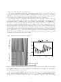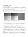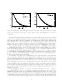
Download 1.5M, PDF

SAM COMMISSIONING REPORT
Prepared by: A. Tokovinin
Version: 2
Date: December 3, 2013
File: soar/commissioning/doc/report/samrep.tex
1
Contents
1 Summary
4
2 Process of SAM commissioning
2.1 Design and fabrication of SAM . . . . . . . . . . . .
2.2 Commissioning in the NGS mode . . . . . . . . . . .
2.3 Commissioning in the LGS mode . . . . . . . . . . .
2.4 Telescope time used in the SAM LGS commissioning
.
.
.
.
.
.
.
.
.
.
.
.
.
.
.
.
.
.
.
.
.
.
.
.
.
.
.
.
.
.
.
.
.
.
.
.
.
.
.
.
.
.
.
.
.
.
.
.
.
.
.
.
.
.
.
.
.
.
.
.
.
.
.
.
.
.
.
.
.
.
.
.
.
.
.
.
5
5
5
5
6
3 Performance of the SAM AO system
3.1 Laser guide star . . . . . . . . . . . . . . . . . . . . . .
3.1.1 Laser . . . . . . . . . . . . . . . . . . . . . . .
3.1.2 Beam transfer and diagnostic . . . . . . . . . .
3.1.3 Laser Launch Telescope . . . . . . . . . . . . .
3.1.4 Stabilization of LGS position in the WFS . . .
3.1.5 Laser safety . . . . . . . . . . . . . . . . . . . .
3.2 High-order AO loop . . . . . . . . . . . . . . . . . . .
3.2.1 Wave-front sensor . . . . . . . . . . . . . . . .
3.2.2 Range-gating . . . . . . . . . . . . . . . . . . .
3.2.3 LGS size and return flux . . . . . . . . . . . . .
3.2.4 Interaction matrix and loop control . . . . . . .
3.2.5 Centroid noise and residual errors . . . . . . .
3.2.6 Atmospheric parameters deduced from the loop
3.2.7 Non-common-path errors and focusing . . . . .
3.3 Tip-tilt loop . . . . . . . . . . . . . . . . . . . . . . . .
3.3.1 Acquisition of guide stars . . . . . . . . . . . .
3.3.2 Flux and sensitivity . . . . . . . . . . . . . . .
3.3.3 Bandwidth of tip-tilt correction . . . . . . . . .
3.3.4 Flexure . . . . . . . . . . . . . . . . . . . . . .
3.3.5 Dithers . . . . . . . . . . . . . . . . . . . . . .
3.4 Known problems of the SAM AO system . . . . . . . .
3.4.1 High-order loop . . . . . . . . . . . . . . . . . .
3.4.2 Tip-tilt loop and TCS communication . . . . .
3.4.3 Control of the mechanisms and the laser . . . .
. . .
. . .
. . .
. . .
. . .
. . .
. . .
. . .
. . .
. . .
. . .
. . .
data
. . .
. . .
. . .
. . .
. . .
. . .
. . .
. . .
. . .
. . .
. . .
.
.
.
.
.
.
.
.
.
.
.
.
.
.
.
.
.
.
.
.
.
.
.
.
.
.
.
.
.
.
.
.
.
.
.
.
.
.
.
.
.
.
.
.
.
.
.
.
.
.
.
.
.
.
.
.
.
.
.
.
.
.
.
.
.
.
.
.
.
.
.
.
.
.
.
.
.
.
.
.
.
.
.
.
.
.
.
.
.
.
.
.
.
.
.
.
.
.
.
.
.
.
.
.
.
.
.
.
.
.
.
.
.
.
.
.
.
.
.
.
.
.
.
.
.
.
.
.
.
.
.
.
.
.
.
.
.
.
.
.
.
.
.
.
.
.
.
.
.
.
.
.
.
.
.
.
.
.
.
.
.
.
.
.
.
.
.
.
.
.
.
.
.
.
.
.
.
.
.
.
.
.
.
.
.
.
.
.
.
.
.
.
.
.
.
.
.
.
.
.
.
.
.
.
.
.
.
.
.
.
.
.
.
.
.
.
.
.
.
.
.
.
.
.
.
.
.
.
.
.
.
.
.
.
.
.
.
.
.
.
.
.
.
.
.
.
.
.
.
.
.
.
.
.
.
.
.
.
.
.
.
.
.
.
.
.
.
.
.
.
.
.
.
.
.
.
.
.
.
.
.
.
.
.
.
.
.
.
.
.
.
.
.
.
.
.
.
.
.
.
.
.
.
.
.
.
.
.
.
.
.
.
.
.
.
.
.
.
.
.
.
.
.
.
.
.
.
.
.
.
.
.
.
.
.
.
.
.
.
.
.
.
.
.
.
.
.
.
.
.
.
.
.
.
.
.
.
.
.
.
9
9
10
10
11
12
12
13
13
13
14
15
16
17
18
19
19
19
20
21
21
22
22
22
22
4 Performance of SAMI
4.1 CCD and controller . . . . . . . . .
4.2 Filters . . . . . . . . . . . . . . . .
4.3 Throughput and scattered light . .
4.4 Geometry . . . . . . . . . . . . . .
4.4.1 Distortion . . . . . . . . . .
4.4.2 Pixel scale and orientation .
4.5 ADC . . . . . . . . . . . . . . . . .
4.6 Data reduction . . . . . . . . . . .
4.7 Known problems . . . . . . . . . .
.
.
.
.
.
.
.
.
.
.
.
.
.
.
.
.
.
.
.
.
.
.
.
.
.
.
.
.
.
.
.
.
.
.
.
.
.
.
.
.
.
.
.
.
.
.
.
.
.
.
.
.
.
.
.
.
.
.
.
.
.
.
.
.
.
.
.
.
.
.
.
.
.
.
.
.
.
.
.
.
.
.
.
.
.
.
.
.
.
.
.
.
.
.
.
.
.
.
.
.
.
.
.
.
.
.
.
.
.
.
.
.
.
.
.
.
.
.
.
.
.
.
.
.
.
.
.
.
.
.
.
.
.
.
.
.
.
.
.
.
.
.
.
.
23
23
24
24
26
26
27
27
28
28
.
.
.
.
.
.
.
.
.
.
.
.
.
.
.
.
.
.
.
.
.
.
.
.
.
.
.
.
.
.
.
.
.
.
.
.
2
.
.
.
.
.
.
.
.
.
.
.
.
.
.
.
.
.
.
.
.
.
.
.
.
.
.
.
.
.
.
.
.
.
.
.
.
.
.
.
.
.
.
.
.
.
.
.
.
.
.
.
.
.
.
.
.
.
.
.
.
.
.
.
.
.
.
.
.
.
.
.
.
.
.
.
.
.
.
.
.
.
5 Delivered image quality
5.1 Average DIQ, dependence on turbulence profile . . . . . . . . . . . . . . . . . . . . . .
5.2 Characteristics of the SAM PSF . . . . . . . . . . . . . . . . . . . . . . . . . . . . . .
30
30
32
6 SAM operation
6.1 Observing procedure and overheads .
6.2 Laser Clearing House restrictions . .
6.3 Observing tool . . . . . . . . . . . .
6.4 Programmatic issues . . . . . . . . .
.
.
.
.
.
.
.
.
.
.
.
.
.
.
.
.
.
.
.
.
.
.
.
.
.
.
.
.
.
.
.
.
.
.
.
.
.
.
.
.
.
.
.
.
.
.
.
.
.
.
.
.
.
.
.
.
.
.
.
.
.
.
.
.
.
.
.
.
.
.
.
.
.
.
.
.
.
.
.
.
.
.
.
.
.
.
.
.
.
.
.
.
.
.
.
.
.
.
.
.
.
.
.
.
.
.
.
.
.
.
.
.
35
35
36
37
37
7 Documentation
7.1 The web site . . . . . . .
7.2 User manuals and guides .
7.3 Publications . . . . . . . .
7.4 System design notes . . .
7.5 Technical documentation .
.
.
.
.
.
.
.
.
.
.
.
.
.
.
.
.
.
.
.
.
.
.
.
.
.
.
.
.
.
.
.
.
.
.
.
.
.
.
.
.
.
.
.
.
.
.
.
.
.
.
.
.
.
.
.
.
.
.
.
.
.
.
.
.
.
.
.
.
.
.
.
.
.
.
.
.
.
.
.
.
.
.
.
.
.
.
.
.
.
.
.
.
.
.
.
.
.
.
.
.
.
.
.
.
.
.
.
.
.
.
.
.
.
.
.
.
.
.
.
.
.
.
.
.
.
.
.
.
.
.
.
.
.
.
.
.
.
.
.
.
39
39
39
39
40
41
8 Compliance to requirements
8.1 Performance requirements . . . . . . . . . . . . . . . . . . . . . . . . . . . . . . . . . .
8.2 Requirements which are not met or partially met . . . . . . . . . . . . . . . . . . . . .
42
42
42
.
.
.
.
.
.
.
.
.
.
.
.
.
.
.
.
.
.
.
.
.
.
.
.
.
.
.
.
.
.
3
1
Summary
SOAR Adaptive Module (SAM) is a laser-assisted adaptive optics instrument at the 4.1-m SOAR
telescope. By compensating selectively low-altitude turbulence, it improves resolution at visible wavelengths. The instrument contains a 4Kx4K CCD imager covering the 3-arcmin square field.
After commissioning in the NGS mode, SAM closed the loop with the laser in April 2011. Since
then, after 2.5 years of engineering and commissioning work, a stable operation of the AO system
and imager was achieved. Images as sharp as 0.3′′ were obtained since March 2012 under favorable
conditions of weak high-altitude turbulence which happened on about half of the SAM nights. On
such nights, the typical FWHM resolution delivered by SAM is 0.4′′ in the I band and 0.5′′ in the V
band. The compensation quality is uniform over the field (FWHM variation of few percent). On the
nights with strong high turbulence (which does not necessarily mean poor seeing), SAM brings only
a marginal resolution gain in closed loop and delivers V -band FWHM between 0.6′′ and 1′′ .
The first paper using SAM commissioning data on the globular cluster NGC 6496 was published
by Fraga et al. (2013). It demonstrates that the photometric precision and limiting magnitude in
crowded stellar fields are improved by using the SAM AO system and that good-quality photometry
can be derived from the SAMI images. Technical aspects of the SAM instrument are published in
several conference proceedings.
In the period from March 2011 to September 2013, SAM worked on the telescope for 25.5 nights
in total. Two nights were used for the execution of the first regular SAM proposal by D. Murphy.
On several nights in 2013, mostly during bright time, data on the science verification (SV) program
were collected, with a moderate success. The SAM SV program was announced in January 2013. We
received 16 proposals for a total of 17 h of telescope time (mostly dark) and, so far, could execute only
a small fraction of these programs. The SV period was extended into the 2013B semester. When the
SAM SV program is finished, its results will be summarized and reported. The SAM instrument is
not yet formally accepted by the SOAR observatory.
At present, SAM is offered to the NOAO users and to the SOAR partners.
SAM runs need preparation: switching on and testing the instrument, preparing target lists, and
submitting them for the approval of laser propagation. The night-time operation of SAM became
relatively easy. However, owing to the complexity of the instrumenbt, it can be operated only by
a trained person, definitely not by a visiting astronomer. SAM operator can also take science data
in queue mode, should this be necessary. The science productivity of SAM would be enhanced in a
“flexible scheduling” mode, when a designated block of nights is flexibly shared between SAM and
backup programs depending on the high-atmosphere turbulence strength.
This SAM Commissioning Report covers the laser, adaptive optics system, and imager. It focuses
on the performance metrics and operational aspects determined during engineering and commissioning.
The report does not describe the instrument itself and is not intended as a user guide. Extensive (but
still not complete) technical information on SAM can be found on its web site, where the manuals
and the user guide are posted as well. Available documentation is reviewed at the end of the report.
4
2
Process of SAM commissioning
Facility instruments are normally integrated and accepted before their shipment and deployment at
the telescope, and then commissioned while being fully operational. For SAM, these stages were
mixed together: the instrument went through three phases of on-telescope testing, with changes inbetween and after its deployments. This unusual sequence was caused by the intrinsic complexity of
the LGS-assisted adaptive optics (AO), with associated technical challenges and learning experience.
Moreover, SAM was developed at CTIO, and the engineers who created it could continue working on
the instrument installed in their observatory. It took us a substantial effort and time to make SAM
work properly, and only after reaching this stage the real commissioning became possible. On the
other hand, once SAM started to work, its data could find science use, so the commissioning activity
became progressively mixed with the science verification and regular operation.
Throughout this report, we cite System Design Notes (SDNs) (see Section 7) by their number, as
SDN NNNN.
2.1
Design and fabrication of SAM
In this sub-section a brief history of the SAM project is outlined. It started in 2002, after SOAR board
approved the instrument idea. The first conceptual design of the system was reviewed in Tucson in
April 2003. The original concept was revised and reviewed again on January 26, 2004 in La Serena.
The first version of the functional and performance requirements (FPR) was developed in October
2005; it was later refined and posted as a table on the SAM web site. From the outset, it was planned
first to test the AO part of the instrument with a natural guide star (NGS) and later to commission
the instrument with the laser guide star (LGS).
The preliminary design review (PDR-1) of the SAM AO module was held on December 2, 2005.
The reviewed documentation included integration, installation, and commissioning plans. According
to these plans, the instrument would be installed at SOAR by October 2007 and commissioned a year
later. In reality, the mechanical design presented at PDR-1 was substantially revised afterwards, and
the AO module was integrated in 2008–2009. The SAM LGS system was reviewed at the PDR-2 in
September 2007. However, the design of the laser launch telescope (LLT) was reworked and reviewed
again in January 2009. Mechanical design and fabrication were almost always on the critical path,
determining the pace of the project.
2.2
Commissioning in the NGS mode
SAM was first installed at SOAR in August 2009 in incomplete version, without guide probes and
imager. This experiment tested the AO loop operation in real conditions. It took another year to
finish the AO module, its real commissioning in the NGS mode started in November 2010. Before the
installation of SAM at the telescope, its acceptance tests were done (SDN 7108). The results of the
NGS-mode commissioning (AO operation and tip-tilt guiding) are summarized in SDN 7116.
2.3
Commissioning in the LGS mode
The SAM LGS system was hastily integrated in the end of 2010, in parallel with the NGS commissioning. After its deployment and re-configuration of SAM into the LGS mode (the capability to work
with NGS was permanently lost then), the first laser light was achieved in March 2011, with the LGS
loop first closed a month later.
5
In its first LGS run, SAM demonstrated improved resolution in closed loop on some nights, but
not always. The AO loop worked when the laser spots were small and the return LGS flux was
high, but both parameters varied substantially, preventing reliable operation of SAM. As the ambient
temperature dropped in June, it became apparent that the LLT mirror figure was distorted by its
inserts. In August 2011 the LLT was removed for correcting this problem, to be re-installed in
November. The LGS spots looked better in the following run, but the loop could not be closed for
anther technical problem. Then, in January 2012, we found that the LGS spots were again highly
variable, so the AO loop operated with a variable success. It became obvious that the major factor
enlarging the spots was not the LLT optics, but the man-made turbulence created by the warm
electronics located beneath the LLT.
On March 6, 2012, the LLT worked without cover for one night. It happened to be a night with
calm free atmosphere (FA), enabling for the first time a substantial gain in resolution. It took us one
full year to reach this milestone! Some aspects of the AO control were changed during this period to
improve the stability in closed loop, and SAM demonstrated good performance again on May 8, 2012.
Data on a globular cluster obtained on that night turned out to be scientifically useful and led to the
first SAM science paper (Fraga et al. 2013).
The heat source under the LLT was eliminated by modifying slightly its motor-control electronics.
This work was done in August-October 2012, during the second SAM shutdown. Despite this advance,
the gain in resolution achieved during following SAM run in October 2012 was marginal because of
the strong high-altitude turbulence; better results were obtained in December 2012. Then, in January
2013, another important step towards reliable SAM operation was made by introducing binning in
the wave-front sensor (WFS). This provided a convenient stability margin, and the LGS loop never
diverged again even under adverse turbulence conditions.
During 2011–2012, most engineers involved in SAM worked on other, higher-priority projects
(Blanco TCS and DECAM installation). The progress of SAM was paced, on one hand, by the
telescope schedule and, on the other hand, by the availability of resources to fix problems timely.
2.4
Telescope time used in the SAM LGS commissioning
Table 1 below lists SAM engineering runs, starting from the first LGS light. Its second column gives
approximate number of nights in each run. Time lost to thick clouds and major technical failures is
not included; some of it was recovered by back-up programs unrelated to SAM. The 3rd column gives
median delivered inage quality (DIQ) in the I and V bands, where appropriate, to indicate typical
performance. Comments on each run with emphasis on technical work and repairs follow.
March 2011. First laser propagation. Return flux was tested by imaging with SOI. The AO loop
could not be closed: the return flux in the WFS was low because of too fuzzy spots, the LLT loop did
not work yet.
April 2011. LGS loop closed for the first time (in the NGS mode, then in the LGS mode). The
damaged driver of the LLT M3 was repaired and the LLT loop was closed on the last night. The
guiders were not operational, data were taken with HRCam (with image recentering a posteriori).
Resolution gain in closed loop was demonstrated. There were transparent clouds on 2 nights out of 3.
Shutdown in August-November 2011. The problem with LLT M1 became apparent in MayJune, leading to the shutdown and modifications of the LLT. Before that, the LGS beam was aligned,
its polarisation was tuned. The burned plastic ring in the LLT M2 cell was replaced. Some tests on
the sky were done on June 13-14, 2011, showing LGS size between 2′′ and 3′′ . The noisy power supply
of the SAMI Leach controller was replaced.
6
Table 1: Summary of SAM LGS engineering runs
Date
dd.mm.yy
15-16.03.2011
14,16,18.04.2011
7.12.2011
9-11.01.2012
6.02.2012
6-7.03.2012
10.04.2012
08.05.2012
29-31.10.2012
03.12.2012
28-29.01.2013
26.02,02.03.2013
27.03.2013
21,23.06.2013
26-29.09.2013
Nights DIQ(I/V ) Main results and problems
used
arcsec
2
n/a
Laser propagation, return flux
3
0.5/0.55
First closed loop (without tip-tilt)
Shutdown August-November 2011
1
n/a
DM failed, laser sync problem
2.5
0.5/0.6:
WFS failure, poor seeing
1
n/a
LLT loop problem, clouds
2
0.37/0.48 Good DIQ on 06.03, unstable on 07.03
0.5
n/a
Tuning of LLT-M3 loop
1
0.35/0.59 Good DIQ, focusing, thermal imaging
Shutdown August-October 2012
2.5
0.48/0.63 Poor seeing
1
∼0.5
Software problems
1.5
0.4/0.5
Poor seeing; 2x2 binning in WFS
2
0.38/0.52 Good DIQ
0.5
n/a
Clouds
Shutdown April-May 2013
1
n/a
Clouds
4
0.60/0.67 Poor seeing
December 2011. The LLT was installed and tested. One high-voltage channel of the DM driver
burned, it was fixed by using the spare board in the driver. The acquisition images of the LGS taken
during the night were sharp, but the AO loop could not be closed because the cable that connected
laser sync pulses to the SAM RTC was damaged. One quadrant of the SAM WFS CCD had unstable
bias.
January 2012. The WFS CCD was not working, its controller was replaced for this run by a
loaned one. The SOAR telescope had a de-tuned hexapod, requiring adjustment of the LLT pointing.
On the last night of the run, the hexapod setting changed again, the seeing was bad. The LGS size was
poor and variable between 1.6′′ and 2.3′′ (it became obvious that man-made seeing is the cause). The
loop operated stably when the LGS was under 2′′ and diverged otherwise. Only a moderate resolution
gain with SAMI was achieved in closed loop. Numerous software failures were experienced, including
RTC crushes and the loss of connection to the SOAR TCS. After the run, the size of the laser beam
in the LLT was reduced (it was too big), the WFS centroid algorithm was optimized.
February 2012. One night with degrading seeing and transparent clouds. The AO loop diverged
most of the time. Part of the problem was the LLT loop which could not be tuned because the control
axes were not orthogonal (the failure of piezo-platform causing this problem was detected and repaired
only in August 2012). Software problems and RTC crushes.
March 2012. First successful operation of SAM demonstrating the resolution gain on the first
night. The LLT cover was removed to alleviate the man-made seeing problem. On the second night,
with the cover on, the spots were large again and the loop diverged. The LLT loop still had problems,
software failures persisted. In April, the reason of AO loop divergence was investigated and the
real-time software was modified to correct it.
7
May 2012. Another night of successful SAM operation, with a record resolution of 0.26′′ in I
reached and useful science data obtained. Strong wind helped to evacuate the heat from the LLT,
but did not hinder the SAM operation (except the FWHM non-uniformity over the field). A focusing
procedure was developed. The WFS had again problem in the CCD quadrant. The TurSim failed
sometimes, affecting calibrations. Images of SAM with the thermal camera were recorded to quantify
the LLT heating. In June, the SAMI distortion and field curvature were studied during daytime.
Shutdown in August-October 2012. The LLT electronics was modified to reduce dramatically
the heat source under the LLT. The piezo-platform in the LLT was repaired. The line transformer in
the DM driver which failed in July was repaired. The WFS Leach controller was finally repaired to
fix the bias instability. The laser shutter was installed (it failed earlier and was removed). A broken
pin in the DM signal cable which affected one electrode was found and fixed. The pupil alignment in
the WFS was checked.
October 2012. Unfavorable conditions with strong high turbulence during the whole run allowed
only a marginal resolution gain with SAM, but with a stable loop operation. Increased noise in the
WFS and software problems persisted. The missing Hα filter created a false impression of “UV leak”.
There were problems with guide-star acquisition. A 15-Hz oscillation in the tip-tilt loop was found.
December 2012. Of 3 nights allocated to SAM, only one could be used, after the laser control
was established (a software problem). Intermittent communication with the TCS caused divergence
of the tip-tilt loop and missing information in some FITS headers. Better guide-star acquisition with
a wobble tool was tested. The FWHM was variable, but mostly mediocre.
January 2013. The new operational mode with 2x2 binning in the WFS was implemented and
tested. The tip-tilt loop was tuned to avoid 15-Hz oscillation. Variable SAM performance reflected
variable FA seeing. Software problems (communication and device control) continued.
February-March 2013. Two nights of good turbulence conditions and good SAM performance
(0.38′′ median in I). SAM was operated remotely from La Serena. Data on some SV projects were
obtained, SAMI artifacts and non-common-path errors were investigated.
March-April 2013. Of the two nights in March, one was lost to fixing the LGS problem (remove
burned insect), another was lost to transparent clouds. Some SV data were obtained and dithering was
tested. The two dark nights on April 17-18 allocated to the SAM SV program were lost to hexapod
failure in SOAR. In preparation for the SV run, we discovered pieces of broken mirror inside SAM.
The TurSim was damaged as well and its actuator was later replaced (its dimmer also failed and was
repaired). These repairs effectively meant another shutdown of SAM which lasted till June 2013.
June 2013. On the first night, SAM delivered poor correction, the second night was mostly lost to
the accident. After daytime work, the covers of the Goodman spectrograph were left on the Nasmyth
platform. They fell and collided with SAM, damaging the SAMI dewar and Leach controller. The
SOI filter wheel was installed in SAMI.
September 2013. The longest SAM run (5 nights). The DM transformer failed again and had
to be replaced just before the run. The dewar loaned from SIFS was used, as the native SAMI dewar
was under repair (replacement of the LN2 vessel). Otherwise, SAM worked without major technical
problems, apart from the endemic unreliable device control and communication. One night was lost
to clouds entirely. The FA seeing was variable, but generally mediocre. The source of the parasitic
light in SAMI was discovered.
8
3
Performance of the SAM AO system
In this Section, the performance of the SAM AO system is covered. For reference, main parameters
of the AO system are listed in Table 2; they are discussed further in this Section.
Table 2: Standard parameters of the SAM AO system
Parameter
Laser power
Laser frequency
Range and gate
Loop time/frequency
LGS flux
TurSim flux
WFS stage position
LGS spot FWHM
Centroid noise
Number of corrected modes
AO loop gain/leak
Tip-tilt loop gain
LLT loop gain
3.1
Value
7.5 W
10 kHz
7km/0.15km
2.09 ms/478 Hz
100-400 ke/s
1000 ke/s
16-19 mm
1.3′′ -2.3′′
0.15-0.25 pix
38-40
0.25/0.99
0.015
0.08
Comment
Optical power (internal laser sensor)
Fixed setting
Standard setting, 1.25′′ max. spot elongation
Loop time with 2x2 binning in the WFS
WFS flux per sub-aperture
With range/gate of 7/0.5km and 100% dimmer
Adjust to focus SAMI
Measured on WFS average images
Measured in loop data, 2x2 binning
With reconstructor threshold 0.01
Integrator controller
KC1 parameter
KC3 parameter
Laser guide star
15 km
t=100 µs
7.12 km
t=47.5 µs Range gate end
7 km
t=46.7 µs Range gate start
Next pulse
Time
WFS focal plane
H
Laser plume
L
t=0
Laser pulse (34 ns)
Figure 1: Propagation of the laser pulse (“bullet”) in the atmosphere and range-gating. The “donuts”
depict defocused images of the laser spot in the wave-front sensor (WFS) at different moments in time.
Figure 1 illustrates the creation of artificial laser guide star (LGS) using Rayleigh scattering of a
9
pulsed laser.
3.1.1
Laser
The LGS is produced by Rayleigh and aerosol scattering of light at 355 nm wavelength from the
frequency-tripled Nd:YAG pulsed laser. The laser (model Q301-HD from JDSU) has nominal power
of 10 W. It is located on the telescope truss, in a thermal box maintained at +20◦ C temperature.
In real operation (under variable gravity and at the altitude of Pachón) the internal power meter of
the laser gives output power in the range from 7.5 W to 7.8 W. The beam quality measured in the
laboratory is very good, M 2 = 1.05 (SDN 2314).
The JDSU company fabricated hundreds of such lasers, it is a rugged industrial product. So far,
we had no problems with the laser: it works and does not require any servicing, apart from the coolant
refreshment every year or so. The MMT team had a similarly positive experience with the laser from
this manufacturer.
3.1.2
Beam transfer and diagnostic
The narrow beam emerging from the laser is expanded to the 1/e2 diameter of ∼8 mm and directed
to the laser launch telescope (LLT) with one reflection from the LGS-M4 mirror. The tilts of this
mirror are controlled remotely for centering the beam on the LLT mirror. Four photo-diodes around
its primary mirror and the 5th diode on-axis serve for the beam diagnostic. The tilts of the LGS-M4
are regulated to center the beam by balancing the 4 signals approximately, while the laser beam is
propagated in the dome during daytime (this operation is now automated by the script M4.lua).
Figure 2: Burned insect extracted from the SAM LGS light duct in March 2013. The picture shows
damage to the optical window of the laser box. The insert demonstrates the affected UV beam arriving
in the LLT, with a cross-like shadow. Image on the right shows the beam emitted by the LLT after
cleaning the window (from SDN 7132).
In March 2013, we detected beam anomaly remotely (from La Serena) during routine LGS daytime
test, using the photo-diode signals. It was produced by a burned insect on the exit window of the
laser box (Fig. 2). This incident proves that the beam diagnostic is adequate.
The size of the beam on the LLT mirror is adjusted by the magnification and/or focus of the beam
expander in the laser box. It is measured by the ratio of photo-diode signals and/or by the shape of
the UV beam at the LLT exit, scattered from the paper (this beam is safe). The initial size of the
beam was too large, causing vignetting. It was reduced to the FWHM diameter of 125 mm in January
10
2012 (SDN 7120). With this beam diameter, the readings of the peripheral photo-diodes are around
0.3, while the central photo-diode is at 2.4.
The polarization of the laser beam leaving the LLT must be circular. This is adjusted by the angle
of the λ/4 wave plate inside the LLT. The control is done by a camera with Wollaston prism looking
into the laser beam (SDN 7121, Fig. 1).
3.1.3
Laser Launch Telescope
Much work has been done on optimizing the optics of the LLT which defines the size of the LGS spots
and, by consequence, the performance of the SAM AO loop. After fixing the insert problem in the
primary mirror, the LLT has been thoroughly checked and aligned in October 2011 (SDN 2323). It has
a built-in source of collimated red light and an imager (Alignment-Projector Telescope, ATP). When
the 20-cm flat mirror is placed in front of the LLT, its optics can be controlled in auto-collimation using
either this internal red beam or the UV laser. In auto-collimation, optical aberrations are doubled,
providing a stringent test of the quality.
Thermal test and subsequent use verified that the insert problem indeed disappeared after the
first shutdown. With the red beam, the achieved FWHM of the image in double pass under good
alignment is 0.9′′ . The primary mirror of the LLT has zonal polishing defects (“ripple”) with rms
amplitude of 21 nm. The ripple deflects about 20% of the UV light into a halo of 5′′ − 7′′ radius, so this
light is effectively lost. The expected half-energy diameter of the LGS (including aberrations, ripple,
and seeing on the up-link path) is about 1′′ (SDN 2320). Indeed, LGS spots of this size were recorded
in SAM, but not always (see below).
The auto-collimation test was repeated at the telescope several times, using both the red diode
and the UV laser in reduced-power mode. The misalignment of the beam expander was corrected in
July 2011. See the results in SDN 7118, 7120, 7121, 7124. The alignment was checked again in August
2013, after more than a year of use, and found stable (SDN 7134). In addition, bright stars were
imaged repeatedly through the LLT using the ATP camera and low-order aberrations were evaluated
from their defocused images.
The major source of variable spot degradation was the local turbulence caused by the warm
air inside and near the LLT; it was systematically warmer that the air in the dome and SAM. A
study of environment with thermal camera is reported in SDN 7126. This problem was corrected by
modifications of the motor-control electronic box: now it is powered only during LGS acquisition.
Another box with line transformer and piezo drivers was displaced away from the LLT, to the top
ring. After these modifications, the LLT temperature during the night remains equal or below the
SAM temperature. Yet, the LGS spots still show sporadic degradation. Various heat sources inside
the SOAR dome, partly reported in the SDN 7126, are the likely cause (streams of hot air can cross
the LLT beam sporadically).
The four motorized motions of the LLT (pointing by tilt and translation of the primary mirror,
focus, and environmental cover) worked without failures (only their control software failed sometimes).
The LLT focus is stabilized by the invar rod and does not react to temperature changes. The focus at
infinity is established during auto-collimation tests to be around 0.00 (relative reading). An offset of
+0.025 is needed to refocus the LLT to 7 km distance. The LLT focus was refined during observations
by examining the LGS spots in the WFS or ACAM.
The pointing range of the LLT is about ±78′′ in X (left-right) and about ±104′′ in Y (up-down).
The LLT has to be co-aligned with the SOAR optical axis within a fraction of this range to allow LGS
centering. Initially, the co-alignment was done iteratively. After LLT installation, the image of a bright
11
(V < 3 star was acquired in the ATP by a spiral search of SOAR. The coordinates were translated
to the required LLT offset, and the next iteration was done. In 2011, a periscope was constructed
to co-align LLT and SOAR during daytime. The beam of the internal ATP emerging from the LLT
and the beam propagating from SOAR on-axis (it is emitted by the SAM guide probe placed at the
center and back-illuminated by a fiber-coupled laser) are brought to coincidence by observing them
simultaneously with a periscope and tilting the LLT. This method works well, but the SOAR telescope
has to be in a horizontal position where its active optics does not operate normally. The LLT axis
must be offset by 90′′ upwards to compensate for this bias.
The co-alignment between LLT and SOAR depends on the settings of the SOAR M2 hexapod. It
had to be re-adjusted in January 2012 when the hexapod position differed from its nominal value; the
LLT adjustment was restored back during the next run. The LLT axis adjustment is stable in time,
no need to check it if the hexapod is stable.
The PDR-2 review committee expressed some concern about LLT vibrations. No vibrations were
observed even under strong wind up to 10 m/s. The average centroid of all spots has a smooth
spectrum and shows no resonances, only the known 50-Hz vibration of the SOAR itself (see Fig. 5
below).
3.1.4
Stabilization of LGS position in the WFS
Centering of the LGS in the WFS aperture is achieved by fast actuation of the flat dichroic mirror
LGS-M3 inside the LLT, which is mounted on a tip-tilt platform. This system was tuned in April
2011. However, since December 2011 the axes of the LGS-M3 platform became non-orthogonal. As
a result, the control matrix of the uplink tilt had to be modified, and yet the the spot centering
remained problematic, affecting the AO loop stability. During the shutdown in 2012, a broken wire
in the platform was found and repaired. The orthogonality of motions was restored. The feedback
gain was adjusted to KC3 = 0.08, and this loop works very reliably ever since. It “drags” the spots
into the WFS aperture even when they are strongly decentered and barely visible. The LLT-M3 loop
compensates tilts up to 10 Hz (see the residual spectrum below in Fig. 5). The rms residual global tilt
in the WFS is typically < 0.2′′ .
3.1.5
Laser safety
The SAM laser is class IV and requires safety management. However, all intense beams are totally
encapsulated. The beam emerging from the LLT is sufficiently diluted to be safe for skin and eyes.
Moreover, it cannot be accessed from the dome level or from the telescope platforms. Therefore,
the SAM LGS system is class I (safe) during normal operation. Presence of personel in the dome is
authorized and no protective equipment is necessary.
The SAM LGS system is aircraft-safe. Its beam is invisible and cannot cause eye damage, while
its thermal effect on a moving target is well below the safety threshold.
Strict laser safety must be imposed during maintenance of the SAM LGS, when the covers are
removed and intense beams can be exposed. Such maintenance must be done only by qualified personnel wearing protective goggles. Access of other personnel to the dome area is restricted during laser
maintenance, while luminous panels warn that the laser is activated. These panels can be ignored in
normal SAM operation.
To further prevent the risk, the laser is physically disabled by removing a key from its power supply
at all times, except during SAM runs and SAM maintenance or tests.
12
3.2
3.2.1
High-order AO loop
Wave-front sensor
The wavefront sensor is based on the CCD-39 detector from e2v with 80x80 pixels. Each pixel has
a physical size of 24 µm and projects to 0.345′′ on the sky. The lenslet array (LLA) in front of the
CCD defines 10x10 sub-apertures with projected size of 0.4 m on the SOAR pupil. Each sub-aperture
occupies 8 CCD pixels, or 2.76′′ on the sky. The WFS field of view is slightly less, as defined by its
entrance aperture.
Pupil alignment and size. The LLA of the WFS is aligned to the image of the deformable
mirror (DM), which should be conjugated and aligned to the telescope pupil. However, the SAM
instrument rotates in position angle, and if the Nasmyth rotation axis does not pass through the pupil
center, the image of the pupil on the DM will move. This is relevant not only for SAM but for any IR
instruments as well. The SOAR M3 angle was adjusted in November 2010 to diminish pupil motion
on the DM (SDN 7116, Fig. 3; see also SDN 7127, Fig. 1). Pupil co-alignment with the DM and LLA
is now good to within 0.2 of the sub-aperture at all rotator angles. It is checked by measuring the
light flux in all sub-apertures under sky illumination and fitting the model with 3 free parameters:
two lateral displacements and pupil radius.
The pupil radius projected on the LLA should be about 5.1 times larger than the LLA aperture
size, according to the design. In fact it is slightly smaller, about 4.8 apertures (SDN 7133). This causes
a loss of flux in the peripheral sub-apertures and the difference in the AO control matrix between the
TurSim (the artificial light source inside SAM used to measure it) and LGS. The lens that adjusts the
pupil size in the WFS is at the end of its range when the LGS is at 7 km, but can be used to increase
the pupil size for LGS at 10 km and 13 km.
CCD binning by 2x2 is used since January 2013. As the size of the LGS spots is never smaller
than 1′′ , the binned pixel size of 0.69′′ is adequate for their sampling. At the same time, binning
greatly improves the sensitivity because each binned pixel receives more LGS photons. The binning
speeds up the readout (the loop time decreased from 4.3 ms to 2.09 ms, or loop frequency increased
from 226 Hz to 478 Hz). It is still possible to use the 1x1 binning, if necessary.
The average gain of the CCD with 2x2 binning is now 0.50 el/ADU (it was 1.17 el/ADU with 1x1
binning). The rms noise was measured at 11 ADU or 5.5 electrons – same as in the 1x1 regime (the
pixel time did not change). However, during SAM operation the rms noise in the WFS is typically
about 16 ADU. It is apparently increased by some electrical pick-up component which gives regular
patterns in the empty WFS frames (see SDN 7134).
The upper line of the CCD has no sensitivity to light. This is established from the uniformly
illuminated images of the sky. The dead line biases spot centroids in the 4 topmost sub-apertures.
A centroid offset can be introduced to counter-act this bias, which otherwise produces “tails” in the
PSF in closed loop operation.
3.2.2
Range-gating
The distance to the LGS (range) and its vertical extent (gate) are determined by the fast shutter in
the WFS. The shutter is based on the Pockels cell between crossed polarizers. It is opened by short
pulses of 2.4 kV amplitude driven by a timer board in the SAM PXI chassis. The range and gate are
set, then the board is “armed” and starts to open the shutter. The pulses are clocked by the laser in
normal operation or generated by the internal generator during tests.
By increasing the gate, we increase the return flux at the expense of radial spot elongation (the
13
LGS becomes “longer”, and peripheral sub-apertures see it in projection). Spot elongation of few
arcseconds is desirable for optimizing S/N (see SDN 1106), but the small size of the WFS field limits
maximum elongation to about 1′′ .
The closed Pockels cell has a high rejection factor, but still transmits some light after the pulse
because of its internal mechanical oscillations, “ringing” (see SDN 2308). These after-pulses create
weak “tails” of LGS spots which point towards the center. These tails are actually visible only in the
inner sub-apertures, at larger distances from the pupil center they are cut down by the WFS aperture.
3.2.3
LGS size and return flux
20130927T2330
20130930T0254
20130930T0609
Figure 3: Three examples of average images of the LGS spots in the SAM WFS (the time stamps
are given below each image). Left: large spots of 2.3′′ , middle: good spots of 1.3′′ , right: spots with
clouds above 7 km. A slight mis-alignment of the pupil (displecement towards upper-right) is inferred
from the distribution of flux in the sub-apertures.
The size of the LGS spots in the WFS (Fig. 3) is determined by atmospheric turbulence on the
up-link and down-link paths and by the quality of the LGS beam (here we do not account for the
spot elongation, which is an additional geometric factor). It is measured by the standard procedure.
A cube of WFS images in closed loop is averaged, spots in the inner sub-apertures are compressed
along X and Y and fitted by Gaussians; the average FWHM in X and Y is taken as the spot size.
Depending on the ground-layer and dome seeing, it varies between 1′′ (best) to 2.5′′ (worst), with 1.5′′
being typical. The AO loop now works robustly even with large LGS.
The return LGS flux measured by the WFS varies, depending on the LGS size (some light is thrown
outside the WFS aperture), atmospheric conditions (absorption or extra scattering by aerosols), and
rotator angle. The dependence on the rotator angle is caused by the polarization. The LLT beam
is circularly polarized, the Rayleigh scattering preserves the polarization. On the way to SAM, the
polarization is modified by oblique reflections from the SOAR M3 and the fold mirror M4 inside the
ISB, and is further transformed inside SAM. A λ/4 wave plate inside SAM WFS should convert this
light into linear polarization admitted by the Pockels cell. Correct adjustment involves rotation of
both plate and the Pockels cell with its polarizers. The latter functionality is not provided by the
mechanical design of the WFS. The wave plate and Pockels cell were set to the angle determined from
laboratory experiments. It has not been checked at the telescope, and the method of such test is yet
to be developed. Imperfect polarization adjustment of the WFS causes dependence of the return flux
14
on the rotator angle (in other words, light loss).
The typical return flux in SAM operation with LGS at 7 km and gate of 0.15 km is 200 ke/s per
sub-aperture, varying between 100 and 400 ke/s. This means about 400 electrons per loop, which is
sufficient for centroid measurement and leaves ample margin for robust operation of SAM. The laser
power could be less for SAM operation at 7 km, but this excess provides robustness.
An alternative method of measuring return flux and spot size on un-gated images of LGS was
developed in 2011 (SDN 7114). The LGS is a continuous line of light which produces a spot when
the full 4-m aperture of SOAR is focused at some distance in the atmosphere. The FWHM size of
this fuzzy spot is 1.46 times larger than the FWHM of the LGS line (if the line were infinitely thin,
the image would have intensity distribution as 1/r, infinite at the center). This method provides
independent estimates of the LGS spot size which was found to be as good as 1′′ , including the downlink blur (SDN 7118). In the SDN 7114, the return flux is estimated from the energy concentration in
un-gated LGS images obtained with SOI in March 2011. It was found that the total efficiency (uplink
and downlink) was 5%, in good agreement with the estimates of the optical transmission (SDN 1112)
and the lidar equation. This leads to the predicted WFS flux of 600 electrons per 2.1-ms loop, which
is actually observed under favorable rotator angles.
Interaction matrix and loop control
X−slopes [0:71]
Y−slopes [72:143]
3.2.4
DM electrode [0:59]
Figure 4: Interaction matrix: WFS slopes in response to DM electrode poking. The plot on the right
shows IMAT column [47] as recorded on March 25, 2013 (full line) and September 24, 2013 (dashed
line), illustrating stability of the response.
The interaction matrix (IMAT) defines the AO control. It is recorded regularly using the TurSim
light source inside SAM. Each DM electrode is poked by ±5 V and the corresponding WFS signal is
measured (Fig. 4). Comparison with previously recorded IMATs is a diagnostic of the system health
15
(for example, a “dead” DM actuator can be detected). The rms difference between two IMATs is
typically less than 0.2 fraction of their amplitude.
The reconstructor matrix is used to command the DM. It is computed in the RTSoft by pseudoinversion of IMAT with a threshold of 0.01. Typically it leaves 38–40 modes in the reconstructor. Using
a higher threshold (less modes) degrades the compensation quality, while a lower threshold adds weak
modes and degrades loop stability. The fact that a DM with 60 electrodes effectively corrects only
40 modes is explained by the different geometry of the DM (radial) and WFS (rectangular). Note
that with the 40 degrees of freedom, the AO system cannot keep all centroids at zero and, indeed, we
observe a systematic pattern in the average residual centroids (SDN 7130).
The loop control law is integrator with a gain of 0.25 and a leak of 0.99. It is stable with the
2-loop delay between WFS data and correction. With the loop frequency of 478 Hz, the correction
bandwidth at 0 dB level is 16.5 Hz. An alternative, faster controller (Smith predictor) is available,
but it shows excessive high-frequency residuals (jitter) probably caused by unaccounted delays in the
control system. The delay in the RTC was measured in 2005 and found to be a small fraction of the
loop time, but it was not re-measured on the final AO system.
Some modifications to the classical AO control were necessary to stabilize the loop in the LGS mode.
Originally, the loop often diverged by “warping” the DM, so that spots on one side of the aperture
disappeared completely. This was investigated in the SDN 7124. The reason of the instability was the
interaction between the tilt and high-order loops. When some spots disappear (e.g. because of low
flux), their centroids have zero value, but upon subtraction of the global tilt the effective centroids
supplied to the reconstructor are large. The loop attempts to correct this false signal by deforming
the DM and causes further motion of the spots away from the center, hence diverges. The problem
was fixed by using only valid centroids in the high-order reconstructor and in the calculation of the
global tilt. This modification eliminated loop divergence and “warps” of the DM.
Another modification concerns the leak. It is essential for damping the weak un-controlled modes
(otherwise they build up and distort the wavefront). However, the standard approach where the leak
causes control signal to decay towards zero in the absence of fresh slopes was changed. In SAM, the
DM voltages tend to the values which they had upon closing the loop (“flat” DM), and in the absence
of control signal the DM tends to flatten.
3.2.5
Centroid noise and residual errors
During each SAM engineering run, technical data on the AO loop performance were collected. These
data are the sequences of measured slopes and DM commands of 5s to 10s duration, sequences of tilt
error signals and tilt commands, and cubes of WFS spot images (typically 200). Recording of these
technical data was simplified in 2013 (just one-button command). The data are processed uniformly
by a suite of IDL programs which can compute various characteristics. A sample of such data is
presented in Fig. 5.
Originally, the spot centroids were calculated in SAM by the cross-correlation algorithm, using a
template of 2-pixel (0.7′′ ) width. However, the real loop data with larger spots were used to show that
this algorithm is not optimal and that the classical un-weighted centroid gives the smallest error in
SAM (SDN 1305). Depending on the spot size and return flux (both are variable), the rms centroid
error varies between 0.15 and 0.25 binned pixels. It can be a factor of two smaller (0.035′′ ) under good
conditions and with 1x1 binning. The plot in Fig. 5 shows rms centroid variance in each sub-aperture
after subtracting the global tilt. Note the increased centroid noise in some sub-apertures, e.g. in X
for apertures 18, 28, 36, 44. These are the 4 leftmost apertures near the pupil border, affected by the
16
input
Defocus a4
residual
Global tilt (X,Y)
Residual centroid rms (X,Y)
20130926T0120
Figure 5: Performance of the SAM AO loop on September 26 2013, 1:20 UT. Top left: spectrum of
Zernike defocus a4 (residual in dashed line, variance 1.2 rad2 ). Top right: global tilt in X (full line)
and Y (dashed line), rms 0.35 pixels. Lower left: average WFS spots (flux 160 ke/s, spot size 1.61′′ ).
Lower right: residual centroid variance in each sub-aperture (X in full line, Y in dashed line) in WFS
pixels, with global tilt subtracted.
spot elongation and by the reduced pupil size. The conditions for this data set were slightly worse
than average; under good conditions, the centroid noise is smaller and uniform in all apertures, in
both coordinates. The centroid noise is dominated by the measurement errors, while the loop residuals
make only a small contribution.
3.2.6
Atmospheric parameters deduced from the loop data
The SAM real-time software provides real-time estimates of the seeing and AO time constant from
the loop data. These estimates were validated in the NGS mode by comparison with the site monitor.
However, in the LGS mode the measured slopes do not sense the full atmospheric path and characterize
only the ground layers (turbulence power at height h is weighted as (1 − h/H)2 for LGS at height H).
The Fried parameter r0,SAM measured by SAM describes the strength of the ground-layer turbulence
effectively compensated by SAM (seeing in arcseconds ǫ = 0.101m/r0 ). The data presented in Fig. 5
have r0,SAM = 0.20 m. The estimate of the wind speed and AO time constant in the SAM LGS mode
is not very useful and possibly is biased by the centroid noise (to check).
17
3.2.7
Non-common-path errors and focusing
image
model
Figure 6: Long-exposure images in closed loop with intentionally de-tuned LGS range z are recorded
and modeled by the donut algorithm to evaluate residual low-order aberrations. The dependence of
the Zernike defocus a4 on z is a line with a slope of −12.2 µm/km which corresponds to the calculated
slope (from SDN 7125).
The internal aberrations of the SAM optics (including DM) are controlled during daytime by
closing the AO loop on the artificial source (TurSim), recording the “flat” DM shape, and then taking
images of the point source (fiber) behind the guide probe with SAMI. The resulting FWHM resolution
is about 0.2′′ , with some details in the PSF indicative of residual non-common-path aberrations, NCPA
(see SDN 7130). Reaching a better result in the LGS mode is difficult because the two light sources
(TurSim and fiber) are located in different planes and go through different optics. In the NGS mode
of SAM, the NCPA was very small, allowing diffraction-limited imaging of the fiber with a Strehl ratio
of 0.6 (SDN 7108).
The situation is even more complex with the LGS because the LGS spots differ from the TurSim
spots in several ways (spot elongation and truncation, ringing of the Pockels cell, missing upper row in
the WFS CCD). To test NCPA on the sky, we take images of strongly defocused stars in closed loop,
using SAMI. One such test is illustrated in Fig. 6. The “donuts” have some residual structure caused
by the NCPA, but this structure corresponds to high-order aberrations (the “cross” is also seen with
TurSim, e.g. SDN 2325). The low-order terms of NCPA are small, as shown by the donut analysis
(SDN 7125).
Focus is one special NCPA that needs a frequent control. In closed loop, it does not depend on
the telescope focus (which is compensated by the DM), but depends on the LGS range (which can
be influenced by aerosols), focusing of the WFS, and mechanical differences between the WFS and
SAMI paths (including the focus offset produced by filters). We developed a focusing procedure (see
the SAM user guide) where defocused images in closed loop (CL) are recorded, and the best focus is
calculated by linear interpolation, as in Fig. 6. Once the CL focus is determined, focusing in open
loop (OL) is easy: we simply null the defocus a4 measured with the LGS by focusing SOAR, with a
flattened DM.
18
3.3
Tip-tilt loop
SAM has two guide probes (GPs) at the input (un-corrected) focal plane. Each GP is a 2x2 array
of 0.5-mm lenslets that collect square areas of the stellar image and direct the light to the photoncounting detectors (APDs) via fibers. The size of the GP field is therefore 3′′ . Two GPs are used to
provide a better uniformity of correction over the field, and for redundancy. The APD detectors are
fragile, they are switched on only when the telescope is pointed (a hardware overlight protection is
provided as well).
3.3.1
Acquisition of guide stars
Owing to the small field of GPs, acquisition of guide stars is not trivial. The SOAR telescope can
have pointing errors up to 30′′ .1 This error is determined by pre-imaging of the field with SAMI. A
procedure was developed where a star with known coordinates is selected in GMAP, then measured in
the IRAF display of the SAMI image. Once the field offset (FO) is found, the GPs can be positioned
on the selected stars (using the GMAP software).
If the flux of a guide star is not detected after positioning activating the probe, a tool findGP
is used for searching around. It modulates the filed on circles of progressively increasing radius by
applying signals to the SOAR M3 mirror. If a modulation of the flux in GP is found, the star is
detected and the GP is moved towards the star, otherwise it is better to select another star or to
revise the FO.
The GS acquisition procedure critically depends on SAMI and takes most of the overhead time
when pointing a target. The experience shows that it works reliably.
3.3.2
Flux and sensitivity
On a dark sky, the total count of 4 detectors is about 2 and 6 ke/s [check] for GP1 and GP2,
respectively (the APDs in GP2 have a larger dark current compared to GP1). It is calibrated and
subtracted from the signal to allow correct measurement of star flux and error signals. The bias is
higher under bright Moon, then it can be re-calibrated frequently during the night.
The performance of the SAM tt guider is studied in the SDN 7110, based on the results collected
during the NGS commissioning. The stellar magnitudes given in the USNO catalog appear to be very
inaccurate: the relation between the actual flux in the GP (sum of 4 APD count rates, backgroundsubtracted) and magnitudes of the guide stars has a scatter of about 1m rms (Fig. 7). The flux F in
ke/s is related to the stellar magnitude as
F [kel/s] = 100.4(V0 −V ) ,
(1)
with the zero points V0 of 19.9 and 19.7 for GP1 and GP2, respectively. These zero points match the
estimated sensitivity. A star of V = 18m would give a flux of 5.75 ke/s (or 57 events per 10 ms loop
cycle) in GP1. A Gaussian star of 1′′ FWHM (rms width 0.42′′ ) will have a centroid error on the order
of 0.02′′ in the 10-Hz servo bandwidth. Guiding on V = 18m stars was actually done.
The tip-tilt errors are measured by the quad-cell algorithm in dimensionless units ex and ey ranging
between −1 and +1. Their translation into arcseconds depends on the seeing. In the linear part of
the response curve, the star displacement X = ex /R, where the seeing-dependent response coefficient
1
According to S. Heatchote, efforts to improve the pointing model were made, but the problem is in coupling between
the active optics and the mount which is not yet modeled.
19
Figure 7: Total flux in ke/s vs. stellar magnitude for GP1 (left) and GP2 (right). The dotted lines
correspond to the average zero points of 19.9 and 19.7, respectively.
R was measured to be 1.35 arcsec−1 in SDN 7110 by comparing tilt errors measured by the probes
and by the NGS WFS. Alternatively, the response can be measured by scanning one GP through the
star while guiding with another probe.
3.3.3
Bandwidth of tip-tilt correction
Figure 8: Power spectra of the tilt signal from the guide probes before (left, 1101T0658) and after
(right, 1101T0834) the onset of 15-Hz oscillation (from SDN 7127). The servo gain was KC1 = 0.025.
The temporal controller of the tt loop takes into account the frequency response of the correcting
element the SOAR M3 mirror (see SDN 8307) and is designed by assuming R = 1. In fact, under good
conditions the response R becomes larger, the feedback gain of the loop increases, and it starts to
overshoot. Oscillations at a frequency around 15 Hz appear, in agreement with the prediction. Such
oscillations were studied in the SDNs 7110, 7127, 7128 7129. To prevent this from happening, the
20
gain of the tt loop should be set at KC1 = 0.015 instead of the recommended KC1 = 0.025. With
this gain, the tip-tilt correction bandwidth is on the order of 10 Hz, as deduced from the spectra of
recorded signals.
The power spectra of tip and tilt often show a prominent line at 50 Hz caused by the vibrations
of SOAR. The same line is seen in the spectrum of global tilt in Fig. 5, top-right. The data obtained during SAM engineering enable some statistical characterization of the 50-Hz SOAR vibration
(SDN 7111). The rms amplitude of the 50 Hz vibration is between 20 and 50 mas. Its contribution
to the long-exposure PSF is normally negligible, but the effect on diffraction-limited imaging using
speckle interferometry is quite strong, leading to the substantial loss of resolution or sensitivity.
3.3.4
Flexure
During long exposures, the field is stabilized by the GPs. Any flexure between GPs and SAMI focal
plane will cause an image blur. Moreover, such flexure may affect the acquisition of guide stars,
because the field offset is determined with SAMI.
Figure 9: Displacement of the GP1 image in SAMI caused by the Nasmyth rotation (combination of flexure and DM
ROTFLAT). The numbers indicate position angle of the Nasmyth rotator (from
SDN 7127).
The flexure between the GP1, WFS, and visitor instrument was studied in SDN 7116 and found
to be within specs. In SDN 7127 this study was repeated for SAMI (Fig. 9). The total range of
the flexure is only ±0.35′′ , too small to affect the guide-star acquisition. If the rotator angle changes
substantially during series of science exposures, they must be shift-aligned before recombination. For
various reasons, exposures longer that 10-min. are not recommended.
3.3.5
Dithers
A capability to move the science target on the detector (dither) is implemented in SAM. The dither
script opens the tt loop, moves the two GPs, offsets the telescope, and closes the loop again. Each
dither takes about 15 s. Dithers were tested in SDN 7134; an error in the script was corrected later,
now it should work at any position angle. An alternative way of dithering was tested in September
2013: both GPs can be moved by small steps without opening the tt loop.
21
3.4
Known problems of the SAM AO system
This sub-section summarizes known problems of the SAM AO system. As stated above, the AO loop
works stably, so these problems do not prevent robust operation of SAM and occur infrequently.
3.4.1
High-order loop
The high-order loop of SAM works reliably without divergence since May 2012, when the last corrections to the control algorithm were implemented. It became robust under poor seeing conditions since
2x2 binning was implemented in January 2013. At the same time, the real-time computer (RTC) was
upgraded, eliminating crushes of the real-time AO software that happened repeatedly with the old
RTC.
The AO loop fails when something is not done correctly, for example if the high-order loop is closed
before the LLT loop. On March 3, 2013, the IMAT was not measured correctly, and this resulted in
the excessive high-frequency noise in the loop.
Centroid bias caused by the spot elongation and truncation and by the missing signal in the upper
line of the WFS CCD produces a deformation in the DM. This was the case on February 27, 2013,
when the PSF had “tails” on one side (SDN 7131). This was corrected by introducing centroid offsets
in the affected sub-apertures.
The WFS controller can take only a large, but limited number of frames 223 − 1 = 8388607. When
the limit is reached, it stops, and the AO loop “freezes”. This happens without any warning. To
recover, open the loops, reset the WFS, and close the loops again. It is a good idea to reset the
WFS by opening/closing the AO loop between science exposures of a long series (this resets the frame
count). The maximum operation time after reset is 4h50min.
3.4.2
Tip-tilt loop and TCS communication
This loop works reliably. The 15-Hz oscillations observed on some runs resulted from the excessive
loop gain.
Occasionally, the tip-tilt loop suddenly diverges. This happens when the information on the SAM
position angle from the TCS is wrong. This phenomenon is common to all SOAR instruments, it
should be fixed by the SOAR TCS upgrade.
The communication between SAM and TCS is essential for many reasons: information on the
telescope position and rotator angle, commands to the SOAR M3 and mount for guiding, telescope
offsets, and laser safety. Sometimes this connection fails, for reasons unknown. In these situations
SAM cannot operate.
3.4.3
Control of the mechanisms and the laser
The SAM AO module and its laser system contain more than 20 remotely controlled mechanisms.
The control of these mechanisms is not very reliable and fails systematically, possibly as a result
of poor communication between software and device controllers. This presents problems during GS
acquisition (the probes refuse to move) and LGS acquisition. Two good nights in December 2012 were
lost for SAM engineering because the laser could not be controlled. So far, we were able to fix the
motion-control problens by opening the engineering GUIs and stopping or re-initializing the motors.
However, until this aspect of the SAM software is fixed, the instrument is not in a working state and
cannot be handed over to regular operation.
22
4
4.1
Performance of SAMI
CCD and controller
SAMI dewar contains the CCD detector CCD231-84 manufactured by e2v. It is back-illuminated
with astro broad-band AR coating and quantum efficiency around 90% between 500 nm and 700 nm
(manufacturer’s data). The format is 4096(H)×4112(V) pixels continuous (not a mosaic). The physical
pixel size is 15×15 µm or image area 61.4×61.4 mm.
The CCD is read out through 4 amplifiers using the SDSU-III (“Leach”) controller. The image is
written in a multi-extension FITS file. The readout time of the full frame with 2x2 binning is about
8 s, the gain is 2.1 electrons per ADU, and the readout noise is about 4 el. Pattern noise is absent.
The blade shutter of SAMI can realize exposures as short as 0.1 s.
Figure 10: Dome flats fields with 2x2 binning recorded on March 2, 2013. Left: V-band, center:
R-band, right: ratio V/R.
Figure 10 shows dome flats recorded with SAMI on March 2, 2013 with 2x2 binning. Small dark
spots common to the filters V and R are caused by the dust particles on the dewar window (it has
not been cleaned properly). Larger spots are caused by the dust or defects on the filters. In the ratio
of those two flats, the difference in the gains and the dust on the window are compensated, while the
dust on the filters is not, causing variations on the order of 2%. These images demonstrate very good
cosmetic quality of this CCD; it does not have bad columns or other blemishes.
Figure 11 illustrates noise in the bias frame (also data of March 2, 2013, 2x2 binning). Subtraction
of the overscan levels leaves a tiny (about 1 ADU) difference between left and right halves of the CCD
(a larger difference with a vertical gradient was found in September 2013 while using a similar loaned
dewar at SAM, see SDN 7135). The plots show power spectra of the bias frame along the line, for
each quadrant (the quadrants 0–3 correspond to the image extensions 1–4). The numbers on the plots
show the “noise floor” in ADU calculated from the level of the “white noise” (without considering
periodic components). The rms signal fluctuations in the overscan areas are around 2.24 ADU, in all
quadrants.
The gain was determined to be 2.1 el/ADU during laboratory tests. This value is confirmed by the
fluctuations of the ratio of two flat fields. The readout noise is therefore about 4.7 electrons. The gains
in all quadrants are equal to within few percent. In fact, relative gains were determined accurately
from the “steps” in the flat fields and are [0.997, 0.980, 1.033, 0.989] in quadrants 0–3, respectively.
23
1.39
1.65
Q2
Q0
1.77
Q3
2.18
Q1
Figure 11: Bias and its noise in 2x2 binning mode (data of March 2, 2013). The plots show averaged
power spectra of signal fluctuations along CCD lines in each of four quadrants, the numbers are noise
floor in ADU.
The readout time of the full frame with 2x2 binning is 10 s (pixel time 2.320 µs). A region of
interest (ROI) can be selected, but this functionality has not been used in the observations so far.
The charge transfer efficiency is very good, > 0.999997 per transfer (laboratory data). The linearity
in the fast readout mode was tested in the laboratory (better than 0.5%), but in the normal mode
used in SAMI it remains to be verified. The full well is > 200 kiloelectrons or > 95 kADU. Therefore,
the linearity range is limited by the 16-bit signal coding rather than by the CCD full well. Heavily
saturated images of bright stars show charge bleeding (see Fig. 12 below).
4.2
Filters
SAMI has one filter wheel holding 7 filters of 3x3 inch size. This wheel contains the BV RI filters from
the CTIO collection. Their transmission curves are given in the SAMI manual.
A filter wheel from SOI (4 positions, 4x4-inch filters) is compatible with SAMI. In fact the SOI filter
wheel #1 was used in the SAM runs in June and September 2013, with the SDSS and narrow-band
filters.
4.3
Throughput and scattered light
The internal transmission of the SAM optics in the science path at 632 nm is 90% (SDN 7108, acceptance tests).
L. Fraga compared relative efficiency of SAMI and SOAR Optical Imager, SOI. The gain of SOI
is 2.0 el/ADU, similar to that of SAMI, so the direct comparison of the ADU counts per second is
meaningful. The results are listed in Table 3. Its last column gives the ratio of filter transmissions, as
determined by the measured transmission curves (the I filter in SAMI was not fully characterized).
24
Table 3: Efficiency of SAMI relative to SOI
Filter
B
V
R
I
Rel. eff.
0.71 ± 0.03
1.01 ± 0.02
1.58 ± 0.05
1.16 ± 0.02
Filter ratio
0.77
0.85
1.15
–
We see that lower efficiency of SAMI in the B band is mostly explained by the lower filter transmission, while in other filters SAMI is more efficient than SOI. The gap in the CCDs of SOI further
increases the effective exposure time of the latter by the need to do mosaicing.
Another way of expressing the SAMI throughput is by giving the zero points: magnitude of stars
that give counts of 1 ADU/s. Calibration with photometric standards (Fraga et al. 2013) leads to
the zero points of [25.06, 25.48, 25.79, 25.16] in the B, V, R, I bands, respectively. Zero points in the
SDSS filters will be determined from the data of the September 2013 run.
Figure 12: Characterization of scattered light in SAMI. The 40-s exposure of HIP 6712 (Sep. 26,
2013, image #131, i′ filter) contains the heavily saturated image of the bright primary component and
the secondary component at 24.4′′ separation, 7.5m fainter. The plot on the right shows vertical cuts
through both components, scaled to the measured or estimated central intensity.
The scattered light in the SAMI images is dominated by the usual effects (reflections from the
dewar window and filters, diffraction on the SOAR spiders). The optics of SAM does not add any
ghosts and may only contribute extra faint “rays” comparable to the intensity of the diffraction spikes.
In Fig. 12, we plot vertical cuts through two components of a wide binary. The image of the primary
component (IC = 7.38) is heavily saturated and bleeding. The secondary is estimated to be 7.5m
or 1000 times fainter than the primary in the SDSS i′ band. It is located at 24.4′′ separation. The
background around the secondary (dashed line) is 10−2 of its central intensity, or 10−5 of the primary
intensity, in agreement with the scaled profile of the primary itself. The profile of the PSF at levels
above 1% of the maximum corresponds to the Moffat function with β = 2 (see below).
25
4.4
Geometry
When the SAM position angle is zero, the +Y axis of the CCD points North, +X points West. To
display the SAMI image in standard orientation (X to the East), invert the X-axis of DS9. For nonzero PA, add PA to get the true-North angle w.r.t. +Y (counted positive CCW). For PA=90◦ , North
points to +X, East to +Y (SDN 8250).
4.4.1
Distortion
Figure 13: Effect of distortion correction on the astrometric solution. Positions of the 2MASS sources
in the crowded field are shown. The image on the left is before distortion correction, the circles are
displaced up and left in the corners and down-right at the center, the rms residuals are 0.5′′ . On the
right, the distortion is corrected (note the thin dark band on top of the frame), the rms residuals are
0.17′′ . The red arrow points Pluto (image #097 of Sep. 26, 2013).
The re-imaging optics of SAM (two off-axis parabolic mirrors) introduces a substantial distortion in
SAMI. The maximum displacement of sources in the corners of the CCD are about 1.8 mm (SDNs 2325,
8250, 7131).The distortion displacement is symmetric about the CCD center (in the same direction)
and depends quadratically on the distance from the center. It was measured twice using light sources
in the GP as probes. Add following corrections to the measured pixel coordinate to translate them
into a virtual distortion-free frame:
∆px = cxx X 2 + cxy Y 2 ,
∆py
= cyx
X2
+ cyy Y
2,
cxx = 2.15E − 6, cxy = 1.99E − 6
cyx = −4.24E − 6, cyy = −4.37E − 6
(2)
(3)
Here X, Y are distances from the CCD center, in un-binned pixels.
There are two ways of correcting distortion. If dithered images are to be combined, they must be remapped on a regular (undistorted) pixel grid. This can be done with the IDL program samiwarp.pro.
It also works on the binned images and writes the result in a file with a prefix d. Linear interpolation
26
between pixels spreads cosmic-ray events and modifies the noise properties (a “moire” modulation of
the noise variance appears). Alternatively, the image can be left without re-mapping, but a non-linear
astrometric solution can be fitted to stars with known coordinates.
A side effect of the distortion is a varying pixel surface. It biases the fluxes of point sources (stars)
in the flat-fielded images. The bias is proportional to the Jacobian of the coordinate transform and,
in the case of SAMI’s quadratic distortion, equals 1 + 2cxx X + 2cyy Y . In the corners, this correction
reaches ±2.7% (see SDN 2325).
4.4.2
Pixel scale and orientation
Astrometric solution can be obtained with the quickastrometry tool by D. Perry, adapted to SAMI
by L. Fraga. The script samiqastrometry.py works together with sextractor and writes WCS
keywords to the FITS header (the new image is prefixed with a, as explained in the SAMI manual).
Good solution is obtained only on distortion-corrected images (see Fig. 13). Application of this tool
to 3 objects observed on Sep. 26, 2013 (SDN 7135) gives consistent results. The binned pixel scale is
0.0909905, 0.0909909, and 0.0909918 arcsec. The mean 0.090991 arcsec/pixel corresponds to the focal
length of 68.006 m. The scale may depend slightly on the SAM temperature and installed filters, as
they influence the mapping between the SOAR focal plane and the CCD.
The +Y axis of the CCD is parallel to the +Y axis of the guide probe stages to within 0.14◦
(SDN 2325); this angle may change a little when the dewar is re-installed or when a loaner dewar is
used in SAMI. The angle between +Y and true North determined by samiqastrometry.py seems to
vary between runs and targets, reflecting imperfect adjustment of the SOAR rotator and errors of the
SOAR pointing model. In September 2013, this angle was +0.8◦ .
4.5
ADC
Figure 14: Image shift produced by two ADC prisms in combination as a function of their relative
half-angle (0◦ at zenith, 51◦ at the zenith distance 60◦ ).
Atmospheric dispersion corrector (ADC) of SAM consists of a pair of two zero-deviation prisms.
27
It can be inserted in the collimated space of SAM. The prisms were fabricated according to specs, but
not glued precisely (even after being returned to the manufacturer and repolished). As a result, ADC
introduces some deviation in the image position, depending on the zenith distance and orientation
(Fig. 14, see also SDN 7108). This has two consequences. First, the determination of the field offset
with SAMI is affected at a level of ∼ 2′′ , so the acquisition image should be taken without ADC. Second,
ADC adjustment during exposure would shift the image (it is not tracked by the guide probes). So,
the tracking mode of the ADC must not be used. It should be set to correct angle before the exposure
and left fixed. So far, ADC was not used with SAMI.
The ADC angle and strength of the compensation were tuned accurately in the speckle regime,
using HRCAM. Diffraction-limited imaging is achieved, so the correction is more than adequate for
SAMI. So, the ADC is tested and ready to be used, when needed.
4.6
Data reduction
The images are recorded as multi-extension FITS files, one extension per amplifier. The headers
contain some information on the SAM state (e.g. open or closed loop). Their content will be enhanced
in the future by adding the positions and coordinates of the guide stars, pointing offsets, etc.
The dome and sky flats and bias frames should be taken together with the data for standard CCD
reductions. The reductions for a night of data are done by the python script samipipe.py working
in pyraf and developed by L. Fraga. The reduced images are combined in single-extension (standard)
FITS files with prefix mzf. These data are delivered to the proposers (so far, by FTP) for further use.
4.7
Known problems
UV leak. Laser light scattered by the air in front of SOAR creates an intense background at 355 nm
wavelength. Most of this UV light is reflected by the dichroic in SAM towards the WFS, but a fraction
still reaches the SAMI CCD. The B filter transmits some of this light. This UV leak is seen as a dark
“cross” in the center of deep B-band exposures (SDN 7131, Fig. 8). The “cross” is produced by
the shadow of the SOAR spiders, it rotates together with SAM. The leak is much smaller, but still
perceptible, in the SDSS g filter. The prospect of modeling this background is unlikely, given its
dependence on such variable factors as atmospheric aerosol and rotator angle.
Dome flats do not match sky flats and leave details in the sky background. Figure 15, left,
illustrates this effect caused by the gradient of pupil illumination in the dome flats. For precise
photometry, sky flats are essential.
Parasitic light in the V or SDSS r filters produced a gradient in the background which decreased along the X-axis of the CCD (Fig. 15, right). In September 2013, the source of this light was
tracked down to the wavefront acquisition camera inside SAM. The camera can be switched off during
exposures, so this problem will not reappear. The existing data were corrected by subtracting the
contribution of parasitic light in the filter r.
Crashes of SAMI GUI happen regularly, maybe once every night. Yet another problem is
“hanging” of the VNC connection to SAMI, which restores itself after a ∼ 60 s timeout. The document
describing the functionality of the SAMI software (a clone of the SOI software with minor modification)
does not exist.
28
Figure 15: Caveats in the SAMI data. Left: division of sky flat by the dome flat in the SDSS r filter.
Right: contours of the parasitic light in the r filter (counts in 5-min. exposure).
29
5
Delivered image quality
5.1
Average DIQ, dependence on turbulence profile
Figure 16: Median FWHM in closed
(full line) and open (dashed line)
loop for the night of March 6/7,
2012, as function of wavelength.
Cerro Pachon, 26/27 Feb 2013
Cerro Pachon, 02/03 Mar 2013
1.5
1.5
DIMM seeing
FA seeing
FWHM (I)
Seeing, arcseconds
Seeing, arcseconds
DIMM seeing
FA seeing
FWHM (I)
1
0.5
0
0
2
4
6
8
1
0.5
0
0
10
UT, hours
2
4
6
8
10
UT, hours
Figure 17: Atmospheric conditions and DIQ on two SAM nights. The black lines show the total
(DIMM) seeing, the red lines the FA seeing at zenith. The blue dots are average FWHM of closedloop images in SAMI (I filter, no correction to zenith).
The resolution in closed loop reached by SAM on its first successful night, March 6/7 2012, is
typical of its performance on other similarly good nights. Figure 16 compares the median delivered
image quality (DIQ) – FWHM of the stellar images – in open and closed loop, as a function of the
wavelength. The compensation quality and gain in resolution (compared to open loop) is better at
longer wavelengths. The turbulence strength and profile do not depend on the wavelength, of course,
but the degree of turbulence compensation does. A ground-layer AO system of higher order would
perform better in the blue region of the spectrum.
When most of turbulence is located above few km, SAM in closed loop brings little or no gain
in resolution. Recall that SAM senses turbulence with a height-dependent weight proportional to
30
(1 − h/H)2 because of the cone effect. For example, a turbulent
layer at h = 2 km is sensed with a
√
weight 0.5. Its full compensation would reduce the seeing by 0.5 = 0.7, but the actual compensation
is always partial and the gain will be even less. SAM effectively corrects turbulence located below
0.5 km and in the dome.
Figures 17 and 18 show SAM performance on two nights in February-March 2013, when the AO
system worked with 2x2 binning. The data from the Pachón site monitor are plotted for comparison.
The full seeing measured by DIMM was between 0.8′′ and 1.5′′ , the seeing in the free atmosphere
(FA) above 0.5 km measured simultaneously by the MASS instrument, plotted in red, varied between
0.3′′ and 1′′ . The DIQ of SAM in closed loop, determined by automatic procedure on all images in I
filter (except focusing tests) is plotted by blue dots. Even without correction to zenith, it follows the
free-atmosphere seeing quite well. On February 26/27, poor SAM performance was expected after 6h
UT (when other instrument was used at SOAR), as indeed was observed on other nights with strong
FA turbulence (see the median values in Table 1).
The median FA seeing at Cerro Pachón is 0.4′ according to several years of MASS data (Tokovinin
& Travouillon, 2006, MNRAS, 365, 1235). It roughly corresponds to the median DIQ in SAM delivered
on 50% of “good” nights in the I band. The FA seeing depends on seasons, being worse during winter.
This is related to the higher wind speed in the upper atmosphere. Predictions of the wind speed
at 200 mB preessure level (about 12 km a.s.l.) are available a week ahead from the global circulation
models. We consulted these prognostics made by ESO for La Silla and found them useful in evaluating
the chances of good SAM performance in the forthcoming runs. It might be useful to have a tool for
extracting the predicted 200-mB wind speed at Pachón to support SAM operation. Meteorological
forecasts are used by Gemini for operating conditions on the mountain, so there may be some synergy
with SAM.
Figure 18: Cumulative histograms of the FWHM in closed (full line) and open (dashed line) loop in
the bands I (left) and V (right) for the two engineering nights plotted in Fig. 17. The CL medians
are 0.384′′ in I and 0.515′′ in V , the OL medians are 0.645′′ and 0.713′′ , respectively.
It is difficult to determine the resolution gain of SAM. Comparison between closed-loop (CL)
and open-loop (OL) DIQ has to be done with careful focusing, DM flattening, and guiding (e.g. by
opening the loop and focusing after taking CL data). However, some existing OL images refer to
photometric standards observed without these precautions. It makes little sense to compare SAM
DIQ to the DIMM seeing because DIMM is often affected by local turbulence and gives pessimistic
31
seeing measures. The FWHM resolution can be improved by SAM by a factor ranging from 1 (no
improvement) to 2 in the I or i bands, and progressively less at shorter wavelengths.
Figure 19: Composite color image of planetary nebula NGC 2440 observed on February 26/27 2013
at UT 2:10 (fragment). The R,G,B colors correspond to the Hα, V , B filters, with 60-s exposures in
each filter and the FWHM resolution of 0.36′′ in B and 0.28′′ in I.
When both FA and ground-layer seeing are good, SAM can reach good resolution even in the B
band, as illustrated in Fig. 19. The DIMM seeing at the moment of these observations was 0.75′′
(cf. Fig. 17), obviously over-estimated. Although little ground-layer turbulence was left for SAM to
correct in these conditions (RTSoft measured ground-layer seeing of 0.5′′ ), its use was fully justified
because it corrected residual optical aberrations, dome seeing, and defocus. Such sharp images have
never obtained at SOAR without SAM. This opens unique opportunities for studying morphology of
deep-sky astronomical objects.
5.2
Characteristics of the SAM PSF
Even without AO correction, the long-exposure PSF has a non-Gaussian profile. Normalized PSF is
frequently approximated by the Moffat function
I(r) = [1 + (ar)2 ]−β ,
p
(4)
where FWHM=(2 21/β − 1)/a, while larger β means weaker wings. The case β = 1 corresponds to
the Lorentz profile, the seeing profile under Kolmogorov turbulence is modeled by β ≈ 4.77.
Modeling of the SAM PSF in the NGS mode is covered in the SDN 7112, where it was found
that the PSF has a peak+wings shape and corresponds to β between 1.0 and 1.5. The LGS PSF was
modeled in SDN 7123. In the LGS mode, the PSF is less peaked, being broadened by the uncorrected
FA turbulence. Figure 20 shows two examples where the PSF is well modeled by the Moffat function
with β = 2, down to 1% level. The best-fitting values of β can be both less and larger that 2, depending
on the conditions.
32
Figure 20: Radial profiles of the PSFs (pluses) and fitted Moffat models (dashed lines) for Boomerang
images taken on March 6/7, 2012 (left: V , #288, right: I, #305). The FWHM and β are indicated
on the plots.
The gain from partial turbulence compensation brought by SAM depends on the science goals and
is related to various metrics of the PSF. For photometry in crowded stellar fields, the figure of merit
is the central intensity of the PSF, equivakent to the Strehl gain (see Olsen, K.A.G., Blum, R.D., &
Rigaut, F. 2003, AJ, 126, 452O). This metric is also relevant for energy concentration in a very small
aperture, while energy concentration in larger (comparable to the FWHM) apertures of various shapes
matters for spectroscopy. Here we consider ǫ50 , diameter of the circle containing 50% of the energy.
If the seeing-limited PSF became simply narrower, the knowledge of its FWHM would be sufficient
for calculating all these figures of merit. The PSF in SAM, however, changes its shape. We compared
numerically the Moffat PSF with β = 4.77 (an approximation of the seeing-limited PSF) with the case
β = 2 typical for SAM. When SAM improves the FWHM by a factor of two, ǫ50 improves only by
1.5 times, while the central intensity (Strehl) increases by 2.8 times (and not by 4 times, as would be
the case for homologous PSF shrinking). These estimates give an idea of potential SAM gain under
favorable conditions and at long wavelengths.
The uniformity of the DIQ over the 3′ SAMI field depends on the atmospheric conditions and the
degree of correction. Both the uncorrected high turbulence and the well-corrected ground layer do
not cause PSF variation in the field, but the partially corrected turbulence in the “grey zone” (at few
hundred meters) should lead to the non-uniformity, with a better resolution on-axis (Tokovinin, 2006).
Figure 21 illustrates this effect by two examples taken on the same night. In the left plot, the FA
seeing was slightly degraded by turbulence at 0.5 km (according to the profile measured by MASS),
and it reflects in the slight radial gradient of DIQ. In the secind plot, the correction was better and
more uniform. At longer wavelengths, the resolution gain from SAM is less but the PSF is even more
uniform over the field.
The data of May 8/9, 2012 are en exception. The seeing conditions were very good, leading to
a good DIQ (SDN 7125). However, the data on the NGC 6496 globular cluster show a gradient of
FWHM along X. In the extreme case, the FWHM resolution in the I filter varied between 0.36′′ on the
left side of the CCD to 0.25′′ on the right side (see Fig. 12 in SDN 7125). We suspected some CCD tilt
or misalignment, but the study with guide probes reported in SDN 2325 demonstrated that there was
no tilt. Strong wind (up to 10 m/s) coupled with the slow AO loop (232 Hz with 1x1 binning in the
33
Figure 21: FWHM uniformity over the field. March 2/3, 2013, I band. Left: UT 4:08, 0.369′′ ; right:
UT 7:13, 0.280′′ (see Fig. 17, right).
WFS) possibly caused delay in the correction, so the best compensation was achieved off-axis, in the
“down-wind” direction. In 2013, with the faster loop running at 478 Hz, such effect was not observed.
Note that despite this non-uniformity, the data on NGC 6496 yielded good photometry (Fraga el at.
2013).
In the 2x2 binning mode of the SAM WFS, the spot centroids at one end of the aperture are biased
by the missing CCD line. This effect is amplified by the AO loop and warps the DM on one side. As
a result, the PSF develops little “tails” (see such tails in the images of bright stars in Fig. 19). The
effect was investigated and corrected by introducing compensating centroid offsets (SDN 7131).
34
6
SAM operation
6.1
Observing procedure and overheads
SAM is a complex system. It should be prepared for each run (switched on and checked) by a trained
person. We assume here that this is done and that SAM is up and running, ready to be used at night.
Certain actions are performed in the evening to prepare instrument for the night: load the target lists,
inform the laser clearing house (LCH) of laser propagation, switch on the laser, open environmental
shutters of SAM and LLT, connect to the software and set the parameters. SAM operator works with
one GUI, the Instrument Control Software (ICS).
The SAM user guide outlines the standard observing procedure for a science target, reproduced
below in abridged version.
• Point the target. Take a short “pointing” exposure to determine the pointing offset. The fields
in GMAP and SAMI must be mutually identified and contain a star with known coordinates.
• Acquire the guide stars, close the tip-tilt loops (SOAR M3 and mount)
• Open the laser shutter and acquire the LGS. The un-gated image is observed with the WFS
acquisition camera and centered by moving the LLT primary in X,Y (the LLT motors are
switched on during LGS acquisition).
• Remove the acquisition mirror from the WFS LGS, close the LLT M3 loop and the high-order
AO loop. Record technical data and declare SAM ready for taking science data.
• If required, check focus by taking intentionally defocused closed-loop images and comparing the
FWHM of stars.
• Dither science images as required by the observer.
• Watch for LCH interrupts. Before each interrupt, pause the science exposure and open the
AO and LLT loops. After the interrupt, open the laser shutter, close the loop and resume the
exposure. The tip-tilt loop remains closed.
Most of the overhead on each pointing is taken by the acquisition of the guide stars. The time
required for this depends on the accuracy of field offset, on the availability of the stars, accuracy of
their catalogued positions, experience of the SAM operator, etc. Such factors as field crowding, ease of
star identification on the pointing image, and reliability of the data in the guide-star catalogs influence
the overhead. The LGS acquisition takes less than a minute. Conservatively, the total overhead (from
the beginning of telescope slew to closing all loops) is estimated to be 15 min, although overheads of
10 min or even shorter were reached in practice sometimes.
There is a clear separation of roles between the SAM operator (see the tasks above) and the
observer. The observer defines the data-taking sequence (exposures, filters, dithering), takes the
images, evaluates their quality in real time, and modifies the strategy in function of atmospheric
conditions and actual performance of the system.
35
Figure 22: Cumulative histograms of laser propagation widows for the period September 25 to 30,
2013. Left: open time, right: closure time.
6.2
Laser Clearing House restrictions
SAM operation is subject to the restrictions of laser propagation imposed by the Laser Clearing House
(LCH). This excludes the use of SAM for targets of opportunity and last-minute changes in the target
coordinates. All laser targets must be submitted in advance. The LCH is informed of the start and
end of laser propagation by phone calls.
Requests for the propagation windows are submitted to the LCH in the form of PRM files few days
in advance of observations (minimum time – 24 hours, TBC). The PRM files have a special format,
they are prepared at CTIO using IDL or IRAF programs that use target coordinates for 2000 as input.
In order to assemble all targets for the SAM run and submit a PRM file, the target coordinates must
be communicated to the SAM operator at least 3 working days before the observations. Typically, a
common target list for a few-day SAM run is prepared and submitted to the LCH as PRMs for each
night of the run.
The authorized propagation windows are sent by the LCH to the [email protected] e-mail
alias. They must be loaded in the SAM LCH software before the start of the observations. The
SAM software allows laser propagation (opening the shutters) when the telescope points to one of the
authorized targets in the PAM file within 120′′ (this parameter is defined in the configuration file).
Dithers within this range do not require definition of separate “targets”.
Figure 22 shows the statistics of ∼2000 windows for the longest SAM run of September 25-30,
2013. We consider only those closures when the target was above 30◦ over the horizon (observable by
SAM). There is no correlation of open or close time with the target altitude. The median open time is
45 min, with a large spread (there are both short and long windows). The median closure time is only
5 s, while about 5% of closure periods are longer than 2 min. The duration of the pause during LCH
closures is set, mostly, by the human reaction needed to pause the exposure, open and close again the
loops.
At any time, the LCH can impose blanket closures where laser propagation is not allowed for all
targets. During the September 2013 run, there was one such 5-min. closure. In principle, blanket
closures can last for the whole night (this happened at Gemini) and can be imposed in the last moment
before the observations start.
36
Targets that do not require laser (e.g. photometric standards) can be observed regardless of LCH
restrictions, in open loop.
6.3
Observing tool
Preparation of target lists for the SAM run, submission of the PAM files to the LCH, and information
on LCH opening and closures during observations require suitable software tools. Initial requirements
for this software, the observing tool (OT), are formulated in the SDN 8102. A version of the OT
running under IDL was developed by A. Tokovinin and is described in SDN 8103. A brief description
of its functionality follows.
Target names and coordinates for the epoch 2000 are prepared as text files and ingested in the
IDL internal structure which contains additional parameters such as type of target, program identifier,
magnitudes, potential guide or pointing stars (up to 5 per target), and text comments. Browsing and
editing of this data is done in the GUI.
Targets for the SAM run are selected in the GUI and saved in run files (lists of target names).
Previously saved runs can be loaded. Target lists for the run can be produced by the OT in two
formats: one for the SAM operator (name, coordinates, comments), another for the SOAR TCS
(number, coordinates, epoch). The PRM file for the selected run and specific date can be generated
as well.
For each target, stars from the USNO2 and 2MASS catalogs in the surrounding 5′ square field can
be retrieved from web and displayed. Magnitudes of potential guide stars in the R band are evaluated
from the JHK 2MASS magnitudes and/or given in the USNO catalog. Candidate guide stars can be
selected or unselected, this information is passed to the main target data structure and is reflected
in the lists (the SOAR lists contains all guide stars as well as main targets). The lists can now be
imported in the GMAP software as a user catalog, assisting in the selection and acquisition of guide
stars during observations. There is also an option of loading the DSS image in the same IDL GUI to
help identify the field in the SAMI pointing exposure.
During the observations, the PAM file can be loaded in the OT (this is independent of loading
PAM in the SAM LCH software). In this case, for each selected target its altitude and closure windows
are displayed as a function of UT time.
The OT is still an experimental software run by Tokovinin on his desktop computer. It can be
further developed and/or coded in a different language to become part of regular SAM software.
6.4
Programmatic issues
After 2.5 years of engineering and upgrades, the operation of SAM became almost routine, with a welldefined observing procedure. Yet, SAM remains a complex system and works smoothly only when it
is properly maintained and tuned. Maintenance and preparation of SAM are beyond the scope of its
operator and should be done by the SAM engineer or instrument scientist. This person has a deep
knowledge of the SAM hardware and software and seeks help from other engineers when required. It
is not conceivable to distribute SAM support between electronics, optics, and mechanical engineers
without coordination by a single person who is responsible for the instrument operation as a whole.
The SAM operator controls the laser (including LCH interaction), acquires giode stars, and closes
the loops, proded that the system is in working condition. SAM operator must know the control
software and understand basic functionality of the AO system. A process of training SOAR operators
in SAM has been started. However, it is not yet clear whether they will be able to take up SAM
37
operation eventually. So far, SAM still has frequent failures in the mechanism control and software
and is not ready for transfer to regular operation.
It is not feasible to train visiting astronomers in SAM operation. Their role is to define the
observing strategy, to take the data with SAMI (or other instruments working with SAM), and to
monitor the data quality.
The operation of SAM can be stopped by an unexpected technical failure (e.g. of its DM driver) or
by a last-minute blanket closure by the LCH. Moreover, on nights with strong high-altitude turbulence
SAM does not provide substantial gain in resolution and the science goals of its programs cannot be
reached. Therefore, it is essential to combine SAM with backup programs that use other SOAR
instruments.
The SAM run requires some preparation: submission of the target lists, switching on and checking
the instrument. SAM will most likely be used during runs and will be switched off in-between.
Considering the dependence of SAM performance on the turbulence profile and the associated need of
backup programs, it makes sense to schedule SAM runs for periods that are longer than the allocated
SAM time. During such periods, the joint scientific output of SAM and accompanying programs can
be maximized by flexible distribution of nights between the instruments.
Efficiency of all telescopes improves with queue scheduling. In the case of adaptive optics and
SAM this is even more relevant. The chances that a visiting astronomer will get the 0.4′′ resolution
in the g band with SAM on a given night scheduled in advance (to give an example) are about 50%.
Therefore, SAM will be used more efficiently in a queue-scheduled mode.
38
7
Documentation
7.1
The web site
The SAM web site at:
http://www.ctio.noao.edu/new/Telescopes/SOAR/Instruments/SAM/
is a repository of documentation and other technical materials (drawings, schematics) related to the
instrument. The technical files and System Design Notes (SDNs) are password-protected, the archive
and manuals are open. Some documents are also copied in the DocDb (protected).
The search engine on the SAM site is based on Google and not well tuned (it returns links outside
SAM). An alternative Document navigator provides links related to various sub-systems.
In the following we list relevant documents on SAM arranged by categories.
7.2
User manuals and guides
SAM user guide, V.1 (Aug. 12, 2013)
SAMI Manual (March 13, 2013)
SAM AOM software description (July 2011)
SAM LGS software description (July 2011)
PAM files for SAM LGS observing runs (June 2011)
SAM LLT quick guide (February 2012)
Real-Time Software User Manual (January 2013)
Real-Time Software Programmer Manual (January 2013)
Instrument Control Software User Manual (September 2013, rev. 3.6.0)
Instrument Control Software Programmer Manual (June 2013)
GS3 User Manual (September 2013)
HR camera software User Manual (August 2008)
HR camera Manual (May 2008)
SAM Alignment Manual (January 2009)
7.3
Publications
In inverse chronological order:
1. Fraga, L., Kunder, A., Tokovinin, A. SOAR adaptive optics observations of the globular cluster
NGC 6496. 2013, AJ, 145, 165
2. Tokovinin, A. GLAO in the visible, the SAM experience In: Adaptive Optics for ELT3, Florence,
May 2013 (sciencesconf.org:ao4elt3:12940)
3. A.Tokovinin, R.Tighe, P.Schurter, R.Cantarutti, N.van der Bliek, M.Martinez, E.Mondaca,
S.Heathcote Performance of the SOAR adaptive module with UV Rayleigh guide star. 2012,
Proc. SPIE, 8447, paper 166
4. Tokovinin, A. GLAO4ELT: a trade study and SAM experience. 2011, Conference AO4ELT2
(Victoria, Canada).
39
5. A.Tokovinin, R.Tighe, P.Schurter, R.Cantarutti, N.van der Bliek, M.Martinez, E.Mondaca,
A.Montane, W. Naudy Cortes SAM sees the light. 2010, Proc. SPIE, 7736, paper 7736-132
6. Tokovinin A. Cantarutti R., Tighe R., Schurter P., van der Bliek N., Martinez M., Mondaca E.
High-resolution imaging at the SOAR telescope. 2010, PASP, 122, 1483
7. A.Tokovinin, R.Tighe, P.Schurter, R.Cantarutti, N.van der Bliek, M.Martinez, E.Mondaca,
A.Montane SAM - a facility GLAO instrument. 2008, Proc. SPIE, 7015, paper 157
8. A.Tokovinin Performance and error budget of a GLAO system. 2008, Proc. SPIE, 7015, paper
77
9. A. Tokovinin, S. Thomas, B. Gregory, N.van der Bliek, P. Schurter, R. Cantarutti, Design of
ground-layer turbulence compensation with a Raleigh beacon. 2004, Proc. SPIE, 5490, 870
10. A. Tokovinin, S. Thomas, G. Vdovin, Using 50-mm electrostatic membrane deformable mirror
in astronomical adaptive optics. 2004, Proc. SPIE, 5490, 580
11. S. Thomas A Simple Turbulence Simulator for Adaptive Optics. 2004, Proc. SPIE, 5490, 766
12. S. Thomas Optimized Centroid Computing in a Shack-Hartmann Sensor. 2004, Proc. SPIE,
5490, 1238
13. Tokovinin A. Seeing improvement with ground-layer adaptive optics. 2004, PASP, 116, 941
14. Tokovinin A., Gregory B., Schwarz H. E., Terebizh V., Thomas S. A visible-light AO system for
the 4.2 m SOAR telescope. 2003, Proc. SPIE, 4839, 673
7.4
System design notes
A large number of documents known as System Design Notes (SDNs) is posted on the SAM intranet.
They are referred in this report as SDN NNNN. The list below contains only SDNs related to the
instrument engineering and commisioning runs.
7101 Optical tests during SAM integration. Jan 7, 2009
7102 SAM commissioning plan. Ap 17, 2009
7103 SAM tests during final integration July 31, 2009
7104 SAM installation at SOAR and first light Aug 11, 2009
7105 First tests of SAM: August 31 to September 3, 2009. Sep 16, 2009
7106 First tests of SAM: October 2, 2009. Nov 11, 2009
7107 Tests of SAM in July 2010. July 28, 2010
7108 Results of SAM acceptance tests. Nov 1, 2010
7109 SAM acceptance and commissioning plan. June 4, 2010
7110 Analysis of tip-tilt data (the January 2011 run). Feb 10, 2011
7111 Dependence on azimuth and elevation of the 50 Hz vibration measured by SAM at SOAR. Feb
23, 2011
7112 Atmospheric parameters and DIQ of SAM in the NGS mode. Feb 16, 2011
7113 LLT tests on February 18/19 2011. Feb 22, 2011
7114 LGS flux measurements in March 2011. Mar 25, 2011
7115 SAM commissioning on April 14-18, 2011. Apr 27, 2011
40
7116
7117
7118
7119
7120
7121
7122
7123
7124
7125
7126
7127
7128
7129
7130
7131
7132
7133
7134
7135
7.5
Summary of SAM commissioning in the NGS mode. May 3, 2011
Tests of the laser beam quality and LLT on June 2-13, 2011. Jun 15, 2011
SAM engineering in December 2011. Dec 12, 2011
SAM engineering in January 2012. Jan 20, 2012
Work on SAM LGS system in January 2012. Jan 30, 2012
SAM engineering on February 6/7, 2012. Feb 9, 2012
SAM engineering on March 6/7, 2012. I. Technical data. Mar 20, 2012
SAM engineering on March 6/7, 2012. II. Compensated images. Mar 15, 2012
SAM engineering on April 10, 2012. LGS tilt control and AO loop instability. Apr 13, 2012
SAM engineering on May 8, 2012. May 15, 2012
Thermal effects of SAM electronics. May 16, 2012
SAM engineering on October 29-31 2012. Nov 20, 2012
SAM engineering on December 1-3 2012. Feb 7, 2013
SAM engineering in January 2013. Feb 7, 2013
Non-common-path errors in SAM (February 2013). Apr 30, 2013
SAM engineering in February 2013. Apr 30, 2013
SAM engineering in March and April 2013. Apr 30, 2013
Test of pupil size in SAM. Jun 11, 2013
SAM engineering in June 2013. Aug 7, 2013
SAM engineering and SV in September 2013. Oct 8, 2013
Technical documentation
Substantial technical documentation is posted on the SAM web site. However, it has not been delivered
fully. Some missing technical documentation is listed below.
SAM maintenance manual
Lists of spares (optics, electronics)
User and programmer guides of SAMI software
User and programmer guides of LCH software
Full set of mechanical drwaings (only main assemblies have PDF drawings, the rest exists in SolidWorks, but is not posted on the SAM web site)
41
8
Compliance to requirements
The requirements are formulated on the SAM web page.2 The engineering requirements were intended
for guiding the design and are not of interest to SAM users. Most requirements are satisfied by the
design of SAM and/or were tested during instrument integration and acceptance. We discuss here
only the top-level performance requirements and the requirements that are not met or need some
comments. The requirements that will not be met after termination of the project are marked by (X).
Some of them turned out to be obsolete or unrealistic, some goals were modified in the course of the
project.
8.1
Performance requirements
G-Perf On-axis FWHM less than 2/3 of uncorrected FWHM. This requirement is met on about 50%
of “good” nights with FA seeing better than 0.4′′ . The typical DIQ in the V band is 0.5′′ , to be
compared to the median seeing of 0.75′′ . The gain in resolution provided by SAM is larger at longer
wavelengths and can reach a factor of two. The sharpest images recorded with SAM have DIQ of
0.25′′ .
G-Perf PSF variation in 3 arcmin. diam. field less than 10% (with two tip-tilt stars). The
correction is very uniform, with FWHM variation of few percent or undetectable.
G-Perf Sky coverage no less than 90% at all Galactic latitudes (with one or two tip-tilt stars). So
far, the sky coverage has been 100% because guide stars were found for all targets.
8.2
Requirements which are not met or partially met
G-Oper-Obs (X) SAM will permit work in queue mode, ready to use even for short periods of good
seeing. SAM is used in the run mode because it requires preparation and is operated by a trained
SAM operator. SAM is switched off between the runs. This requirement was formulated in hope that
the LCH restriction will be waived. It is not feasible with the current LCH procedures. Moreover,
SOAR does not work in queue mode at present.
G-Oper-Obs SAM will measure and display relevant AO data for each acquisition: seeing, atmospheric time constant, estimated compensation quality. The real-time diagnostic provided by SAM
was useful only in the NGS mode. In the LGS mode, the uncompensated high-altitude turbulence
is not sensed by SAM, so its real-time diagnostic, which is still provided, is not related to the DIQ.
Operational turbulence profiler (the MASS channel of the Cerro Pachón site monitor) is needed to
evaluate SAM performance and support its operation.
G-Oper-Maint Diagnostic hardware and software should be included in the design of the instrument. A goal should be that any plausible failure should be localizable to a major module, and hopefully
to a specific electronics card or mechanical subassembly, by tests that can be run remotely by the user.
It should be possible to execute these tests during the day. Specifically, simple loop-back tests should be
available to test communication links independently of higher functions of the modules they interconnect. Errors of communication with individual devices are reported by the high-level GUI. Such errors
happen regularly, therefore more work is needed to provide reliable control of all SAM mechanisms
and the laser. The existing software tools are adequate for localizing the failures, but do not allow
diagnostic of their reasons.
2
http://www.ctio.noao.edu/new/Telescopes/SOAR/Instruments/SAM/pdr/req.html
42
G-Oper-Maint Diagnostic routines to test mechanisms will be provided. No low-level tests of
hardware that could be run automatically were provided.
G-Oper-Maint Manuals and other documentation will be produced for the SAM: Users’ Manual,
Software Manual, Electronics schematics including block diagrams, Mechanical drawings, Interface
document for Visitor Instrument, Maintenance manual. Not all manuals and technical documents are
provided so far (see Sect. 7.5).
G-Oper-Maint SAM will include critical spares. The list of spares is not provided, SAM spares
are not yet ordered and stored properly.
G-Int (X) The maximum mass of SAM+VI will not exceed 340 kg. The mass of SAM is [TBD].
G-Int SAM and its electronics will dissipate no more than 25W into the telescope environment
The heat dissipation is much larger and is not quantified because the SAM electronic boxes, Leach
controllers, and rack are not thermally insulated. Heat generated by the electronics is not effectively
evacuated by the glycol. See thermal images in SDN 7126. Heat generatoin in the SAM LLT electronics
has been reduced.
AO-Opt Optical throughput of the science channel will be no less than 0.85 (goal - 0.88) in the
wavelength range 400 to 1000 nm. The throughput of SAM at 633 nm is excellent, 0.90, but it was
not measured over the full wavelength range. Comparison with SOI indicates, however, that SAM is
as efficient or better (Sect. 4.3).
AO-Opt Optical throughput of the WFS channel at 355nm will be no less than 0.55 (goal - 0.68).
The WFS throughput depends on the rotator angle and varies by a factor of two because the polarization has not been tuned and tested.
AO-Mech Access will be provided to all optical and mechanical components inside SAM bench for
maintenance, cleaning, repair. SAM optics and mechanisms can be accesed only when the instrument
is removed from the telescope and placed on its handling cart.
AO-WFS (X) WFS can work either with NGS at infinity or with LGS at a fixed distance, selectable in the range from 7km to 14km. The dual NGS/LGS mode was abandoned in favor of simplicity, so SAM can no longer work with NGS. The LGS range can be adjusted between 7 km and 13 km,
but is usually kept at 7 km. Longer range can be used only under good conditions because the return
flux is less than at 7 km.
AO-WFS The diameter of the pupil image on the lenslet array will be 1.97 +- 0.02mm. The pupil
image will remain fixed laterally within +- 0.01mm.. The actual diameter of the pupil image is about
1.84 mm, its lateral motion is less than 0.2 aperture diameter or 0.038 mm.
AO-WFS (X) LGS-WFS will contain a fast shutter. Min. exposure time <100ns, rejection in
the 3 arcsec. field no less than 1:100 for one polarization at 355 nm wavelength. The rejection is
less because of the Pockels cell “ringing” (secondary peak of 0.19 amplitude at pulse length of 1 µs,
SDN 2308). This produces additional details in the innermost LGS spots.
AO-WFS The WFS CCD camera can take and read continuous unbinned frames at a rate no less
than 500 Hz. Such a fast readout is noisy and is not used in SAM. With 2x2 bining, the frame and
loop rate is 478 Hz.
AO-WFS The readout noise in the WFS CCD will be less than 10e rms (goal - 6e), without fixed
pattern (white). The CCD RON is 5.5 electrons, but typical rms is about 8 electrons because a variable
amount of electric pick-up noise is added. It creates pattern noise.
AO-WFS The rms centroid errors with LGS will be less than 40 mas. Under good conditions
with 2x2 binning, the centroid noise is 0.15 binned pixels or 0.1′′ . The noise is stronger than planned
because LGS spots are larger than 1′′ .
43
AO-TT The rms tilt error with two R=18 guide stars will be <20 mas. Average residual rms tt
jitter was measured to be 45 mas in SDN 7110. The photon noise error with R = 18m star is about
20 mas (see Section 3.3).
LGS-LLT (X) Aperture diameter 30cm. Reduced to 25 cm
LGS-LLT (X) Strehl ratio at 355nm >0.8 (wavefront errors <25nm rms). Total rms wavefront
aberration is <100 nm rms (high-frequency ripple 21 nm, spherical 30 nm, astigmatism <40 nm), see
SDNs 2323, 2324, 2320.
LGS-Saf (X) The safety shutter will be connected to hardware and software triggers, blocking
the UV laser beam by any alarm signal. As the SAM LGS system is safe in normal operation, this
requirement is not necessary. Blocking of laser emission is provided when laser box is opened.
44