1
LabTool - User’s Guide Copyright 2013 © Embedded Artists AB LabTool User’s Guide EA2-UN-1301 Rev A LabTool – User’s Guide Page 2 Embedded Artists AB Davidshallsgatan 16 SE-211 45 Malmö Sweden [email protected] http://www.EmbeddedArtists.com Copyright 2013 © Embedded Artists AB. All rights reserved. No part of this publication may be reproduced, transmitted, transcribed, stored in a retrieval system, or translated into any language or computer language, in any form or by any means, electronic, mechanical, magnetic, optical, chemical, manual or otherwise, without the prior written permission of Embedded Artists AB. Disclaimer Embedded Artists AB makes no representation or warranties with respect to the contents hereof and specifically disclaims any implied warranties or merchantability or fitness for any particular purpose. Information in this publication is subject to change without notice and does not represent a commitment on the part of Embedded Artists AB. Feedback We appreciate any feedback you may have for improvements on this document. Please send your comments to [email protected]. Trademarks InfraBed and ESIC are trademarks of Embedded Artists AB. All other brand and product names mentioned herein are trademarks, services marks, registered trademarks, or registered service marks of their respective owners and should be treated as such. Copyright 2013 © Embedded Artists AB LabTool – User’s Guide Page 3 Table of Contents Document Revision History 4 1 LabTool Introduction 5 2 QuickStart Guide 9 2.1 Prepare the Hardware 9 2.2 Basic Usage 11 2.3 Interpret Data with Analyzers 14 2.3.1 UART 14 2.3.2 SPI 15 2.3.3 I2C 15 2.3.4 Counters 15 2.3.5 Analog 15 2.3.6 PWM 16 3 Installation 17 3.1 Prepare Hardware 17 3.2 Install PC Application 19 4 Using LabTool 4.1 Start LabTool Application 24 4.2 Setup – Prepare for Measurement 26 4.2.1 4.3 4.3.1 4.4 Copyright 2013 © Embedded Artists AB 23 Project Settings Capturing Export Data Analyzing Captured Data 31 32 33 34 4.4.1 Using Cursors 35 4.4.2 Digital Measurements 36 4.4.3 Analog Measurements 36 4.5 Digital Signal Generation 37 4.6 Analog Signal Generation 39 5 Calibration of Hardware 40 5.1 DC Level Calibration 40 5.2 Analog Input Stage Calibration 43 6 Current Limitations on Application 45 7 Troubleshooting / Things to Know 46 7.1 LPC-Link 2 board is getting hot 46 7.2 A 10 MHz input signal looks distorted 46 7.3 Sample memory usage 46 7.4 LabTool Application cannot find LabTool Hardware 46 LabTool – User’s Guide Page 4 Document Revision History Revision Date Description PA1 2013-01-03 First version. PA2 2013-01-07 Updated with continuous sampling, analog triggering and simultaneous analog and digital sampling. PA3 2013-03-27 Updated for rev PA2 of hardware and updates in GUI. PA4 2013-05-15 Updated for rev PA3 of hardware and ver 0.8 of installation program. Added step-by-step guide to get started. Added description about cursor functionality. PA5 2013-10-14 Updated for rev A of hardware. Added more detailed calibration procedure. General update of document. Copyright 2013 © Embedded Artists AB LabTool – User’s Guide Page 5 1 LabTool Introduction LabTool has been designed to be your best friend on the lab bench! It is a combination of many instruments packed into a compact unit that fits into your palm. 11 channel logic analyzer 2 channel oscilloscope 11 channel digital signal generator 2 channel analog signal generator Details about the performance (sampling rate, resolution, voltage ranges, etc.) of the LabTool instrument are found in the datasheet on the product page. The hardware is built around the LPC4370 microcontroller, which is found on the LPC-Link 2 board. The hardware is the combination of an interface board and the LPC-Link 2 board that is mounted on this interface board, see picture below. LPC-Link 2 board + Interface board Complete LabTool = Figure 1 LabTool Board Structure The user interface for LabTool is software running on a PC. Communication between the hardware and the pc take place over a Hi-Speed (480 Mbps) USB2.0 link. The user interface is feature rich and supports the user in configuration of the system and presenting the captured signals. Below are some screen shots of the user interface, just to give an idea about how it looks. In this document all details about the user interface will be presented. Copyright 2013 © Embedded Artists AB LabTool – User’s Guide Page 6 Figure 2 LabTool User Interface Screenshots As an extra bonus, there are 12 demonstration signals generated by an on-board microcontroller. These are UART, I2C, SPI, PWM and binary counter signals, easily available on 100 mil pitch pin header. The signals can be used to learn how to make full use of the LabTool logic analyzer features and how to work with a logic analyzer in general. The LPC-Link 2 is a debug interface (Cortex debug) and even though the LPC-Link 2 is mounted in the interface board, creating the LabTool, the Cortex debug interface is available and can be used, see picture below. Copyright 2013 © Embedded Artists AB LabTool – User’s Guide Page 7 The picture below illustrates the external connectors on LabTool. USB cable to PC is connected here 12 demos signals, legend on bottom side silk screen Debug interface for demo signal processor (LPC812) Debug interface from LPC-Link 2 – can connect to target microcontroller Calibration signal for analog inputs: upper: 1.25V signal mid: 78mV signal lower: GND 26 cables for Digital I/O and Analog I/O Analog inputs via BNC connectors Figure 3 LabTool Connectors and Interfaces The 26-pos IDC connector carries the following signals. Pin Number Pin Name Cable Color Description of Demo Signal 1 I2C-SDA Green Currently not implemented feature for I2C logging. 2 I2C-SCL Yellow Currently not implemented feature for I2C logging. 3 I2C-VCC Orange Currently not implemented feature for I2C logging. 4 GND Red Ground 5 DIO_VCC Brown Can connect to external logic level reference (2.4-5.5V). If left unconnected, the digital I/O voltage reference will be 3.3V. 6 DIO_10 Black Digital I/O 7 DIO_9 While Digital I/O Copyright 2013 © Embedded Artists AB LabTool – User’s Guide Page 8 8 DIO_8 Grey Digital I/O 9 DIO_7 Violet Digital I/O 10 DIO_6 Blue Digital I/O 11 DIO_5 Green Digital I/O 12 DIO_4 Yellow Digital I/O 13 DIO_3 Orange Digital I/O 14 DIO_2 Red Digital I/O 15 DIO_1 Brown Digital I/O 16 DIO_0 Black Digital I/O 17 GND White Ground 18 AOUT_1 Grey Analog output #1 19 GND Violet Ground 20 AOUT_0 Blue Analog output #0 21 GND Green Ground 22 GND Yellow Ground 23 GND Orange Ground 24 AIN_1 Red Analog/Oscilloscope input #1 25 GND Brown Ground 26 AIN_0 Black Analog/Oscilloscope input #0 The signal names are also written in the silkscreen on the bottom side of the pcb. Odd pin numbers are located on the upper row of the 26-pos IDC connector and even numbers are located on the lower row (closest to the pcb). The use cases for using LabTool in your work are: 11 channel logic analyzer, with/without using the demo signals 11 channel logic analyzer + 2 channel oscilloscope, with/without using the demo signals 11 channel digital signal generator 2 channel analog signal generator 11 channel digital signal generator + 2 channel analog signal generator Cortex Debug interface (SWD) from the functionality of the LPC-Link 2, for example by using the LPCXpresso IDE. As seen it is not possible to both generate and capture signals. Last but not least, the software is released under an open source license. Anyone can contribute and make the LabTool instrument even better! Copyright 2013 © Embedded Artists AB LabTool – User’s Guide Page 9 2 QuickStart Guide There is a Cortex-M0+ microcontroller (LPC812) on the LabTool board that generates some sample signals that are very useful to get started and learn about how to use a logic analyzer. In this chapter you will learn how to take a closer look at them using LabTool and at the same time get a quickstart tour on how to work with LabTool. The guide in this chapter is a quick scratch on the surface to get you started. More complete and detailed information is presented in other chapters. 2.1 Prepare the Hardware Start by following the preparation steps in section 3.1 (preparing hardware, if needed) and then connect the DIO_x/AIN_0 inputs to the demo signals according to this table: Input Cable color Demo Signal (see legend in silkscreen on bottom of pcb) Description of Demo Signal DIO_0 Black UART-TXD Asynchronous UART signal transmitting a string at 115.2kbps, 8N1 (8 databits, no parity, one stopbit) DIO_1 Brown I2C-SDA I2C data signal for communicating with a temperature sensor (LM75) DIO_2 Red I2C-SCL I2C clock signal (250kHz) for communicating with a temperature sensor (LM75) DIO_3 Orange SPI-SSEL SPI device select signal for communicating with an SPI E2PROM (25LC040) DIO_4 Yellow SPI-MOSI SPI slave output signal for communicating with an SPI E2PROM (25LC040) DIO_5 Green SPI-MISO SPI master output signal for communicating with an SPI E2PROM (25LC040) DIO_6 Blue SPI-SCK Clock signal (2.1MHz) for communicating with an SPI E2PROM (25LC040) DIO_7 Violet CNT-QA Counter signal, 1MHz DIO_8 Grey CNT-QB Counter signal, 500KHz DIO_9 White CNT-QC Counter signal, 250KHz DIO_10 Black PWM-LED PWM signal (24kHz) that drives the green LED AIN_0 Black CNT-QD Counter signal, 125KHz Copyright 2013 © Embedded Artists AB LabTool – User’s Guide Page 10 Figure 4 All Demo Signals Connected Legend for the 26-pos cables for Digital I/O and Analog I/O Figure 5 Signal Legends on Bottom Side of PCB Copyright 2013 © Embedded Artists AB Demo signal legends LabTool – User’s Guide Page 11 2.2 Basic Usage The next step is installing the LabTool application as described in section 3.2 The LabTool application can be found on the start menu, see Figure 6, or on the desktop if that option was selected during installation. Figure 6 LabTool Application in Start Menu When the application has started the default screen opens up, as illustrated in Figure 7 below. This window contains a number of areas that are explained below. The left area has a list of the active signals. In the middle area the captured signals are displayed. Between the left and middle areas there is a small area for trigger settings. In the right area the sampled/captured signals are displayed. At the bottom, the cursors are shown and can be manipulated. At the, below the menus, is a toolbar where different settings are controlled, like sample rate, play/capture and time scale adjustment. Copyright 2013 © Embedded Artists AB LabTool – User’s Guide Selected device Active signals Page 12 Sample rate Trigger settings Play/Capture & Stop Time scale control Cursor control area Add signals Sampled/Captured signals Measurements, partly controlled by cursor positions Figure 7 LabTool Application Default Screen A demo project has been installed together with the LabTool application. Select Open in the File menu and point to the demo.prj file which is located in the same folder as LabTool (typically c:\Program Files\Embedded Artists\LabTool). When the project has loaded the first thing to do is to create a new copy of it so that the original is not modified if you want to run this demo again. Select Save As from the File menu as shown in Figure 8. Copyright 2013 © Embedded Artists AB LabTool – User’s Guide Page 13 Figure 8 Save Project Settings The project will be loaded and a number of signals and analyzers will appear, see Figure 9. Play/ Capture UART signal I2C signals SPI signals Counter signals Analog input of a digital signal Figure 9 Demo Project Loaded If the middle area is blank that is because no data has been collected yet. Press the Play/Capture button in the toolbar or select Start from the Capture menu. That will capture a new set of data – one time when the trigger condition is met. Pressing the Continuous Capture button (the infinite symbol, just right of the Play/Capture button) will capture data every time the triggering condition is met – not just one time. Copyright 2013 © Embedded Artists AB LabTool – User’s Guide Page 14 The middle area has a dark background here. This can be changed by selecting another color scheme as illustrated in Figure 10 below. Figure 10 Set Color Scheme 2.3 Interpret Data with Analyzers Now that the project has been loaded and data has been captured, it is time to take a closer look at the different signals and how to interpret the data with the help of analyzers. 2.3.1 UART The LPC812 outputs an asynchronous UART signal at 115.2kbps, 8N1 (8 databits, no parity, one stopbit) on the UART-TXD pin, which is connected to the DIO_0. The message that is sent every second is *** LabTool – temp: xx.x deg. C *** where xx.x is the temperature read from the LM75 temperature sensor mounted on the LabTool board. The default sample rate in the demo is 10MHz which is too high to be able to see the entire signal, see Figure 11 below. Figure 11 Partial Capture of UART Signal There are many ways to capture more of the signal: 1) Lower the sample rate to e.g. 2MHz. This will allow samples to be taken during the entire 3ms duration of the UART message 2) Move the trigger from signal D1/I2C-SDA (default) to D0/UART-TXD 3) Remove all unwanted signals. This will allow the D0 signal to use more memory which results in more samples. 4) Change the post fill settings in Trigger Settings on the Capture menu. By increasing post-fill from the default 50% to e.g. 80% more of the data after the trigger will be saved. Copyright 2013 © Embedded Artists AB LabTool – User’s Guide 2.3.2 Page 15 SPI The LPC812 has an SPI channel where it communicates with an SPI-E2PROM. 4 signals are used, SCK (the clock signal), MOSI (the data signal from master to slave - LPC812 to E2PROM), MISO (the data signal from slave to master – E2PROM to LPC812) and SSEL (the chip select signal, active low). 5) Zoom-in and measure the clock frequency. It should be 1 MHz. Depending on selected sample rate the (time-) resolution might give another value and it can vary slightly between clock cycles. The higher the sample rate, the better resolution and the less jitter in measurements. Hover the cursor over the captured clock signal and read the measurement in the Digital Measurements area, see 4.4.2 on page 36 for more details. 6) It is possible to change settings of an interpreter (reconfigure analyzer) by clicking on the settings icon, see Figure 30 for details where to find it. Experiment with different representation of the data values. Hex is selected in the preloaded project. There are also Decimal and Ascii representation. 7) Observe that the SSEL signal goes low in three different periods. These are The clock signal is high between byte transfers within an active transfer (SSEL low) but goes low in-between transfer blocks (when SSEL goes high). Also note that the bytes are not transferred back-to-back. There is a delay between each byte transfer. Get acquainted with the cursors to measure time periods. Read about how the cursors work and are controlled/manipulated in section 4.4.1 on page 35. 2.3.3 I2C The LPC812 has an I2C channel where it communicates with a temperature sensor, LM75. 2 signals are used, SCL (the clock signal) and SDA (the bidirectional data signal). 8) Zoom-in and measure the clock frequency. It is in the region of 260 kHz. 9) Study the I2C-analyzer output and determine the I2C address of the temperature sensor. The I2C communication takes place in two transfers. Decode what is happening with the help of the LM75 datasheet. 2.3.4 Counters The LPC812 outputs a 2 MHz clock to a 4-bit binary ripple counter. All four signals are available with frequency 1/2, 1/4, 1/8, 1/16 of the input frequency. 3 of them are connected to digital inputs and the lowest frequency signal is connected to analog input #0. 10) Measure the three frequencies. Test to trigger on the lowest frequency signal. Test to trigger on the highest frequency signal. Which one is best for stable reasing. 2.3.5 Analog As presented above, the lowest frequency signal from the ripple counter is connected to the analog input #0. 11) Zoom-in and out and determine the frequency of the digital signal. 12) Verify that the amplitude of the signal seems correct. It is a 3.3V logic signal. Test to change volts/div setting. 13) Test AC coupling of the signal and observe how the signal varies around ground level now. 14) Select continuous sampling and change triggering to the analog signal. Adjust triggering level and verify what happens if outside of the signal range. Also verify that the digital signals just randomly flash by now. The only way to get the back into the “area of interest” is to trigger on UART, SPI or I2C communication signals. Copyright 2013 © Embedded Artists AB LabTool – User’s Guide 2.3.6 Page 16 PWM The last demo signal created by the LPC812 is a PWM signal. It controls a green LED on the board. 15) Measure the PWM-frequency. It is about 24 kHz. Note that the sample frequency must be high to keep stable triggering is the end points (PWM signal almost always high or almost always low). Trigger on this signal. Copyright 2013 © Embedded Artists AB LabTool – User’s Guide Page 17 3 Installation This chapter describes the steps needed to prepare the hardware and install the PC application. 3.1 Prepare Hardware In most cases the hardware is already prepared, looking like the picture below. LabTool can be bought assembled like this. In addition to this, two cables are needed: 26-pos cable for external signals. This cable is included when buying LabTool. USB cable (mini-B to A). Note that this cable is not included when buying LabTool. Verify that no jumpers are inserted on the LPC-Link 2 board. These jumpers can possible be inserted on the bottom side of the LabTool interface board, in the middle hole. Figure 12 Complete LabTool Board If LabTool is not assembled like above, some manual work is needed. The following things are needed (one of each): LPC-Link 2, rev C board LabTool interface board, rev A, with 26-pos cable for external signals. Mounting kit USB cable (mini-B to A) Verify that no jumpers are inserted on JP1 or JP2 on the LPC-Link 2 board, see picture below. Copyright 2013 © Embedded Artists AB LabTool – User’s Guide Page 18 LPC-Link 2 board LabTool interface board No jumpers Figure 13 LPC-Link 2 Board and LabTool Interface Board rev A Place the two boards according to Figure 13 above. Note the board orientations. Place the LPC-Link 2 on top of the LabTool board and press it down – connecting the boards via three connectors. It is possible to mount the two boards slightly misaligned so make sure the connectors on the LPC-Link 2 board are placed symmetrical in the connectors on the LabTool board, see picture below. Symmetrical mounting Figure 14 LPC-Link 2 Board and LabTool Board Mounted When the LPC-Link 2 board has been mounted on the LabTool interface board it will look like on Figure 12 from the top. Copyright 2013 © Embedded Artists AB LabTool – User’s Guide Page 19 3.2 Install PC Application Uninstall any previous installation of LabTool before starting. Make sure the LPC-Link 2 is not connected to the PC via a USB cable during the installation. Run the file Install LabTool vX.Y.exe, when X.Y is the version number to install the software on the PC. Figure 15 First Dialog of Installation Press Next button. Figure 16 Second Dialog of Installation Copyright 2013 © Embedded Artists AB LabTool – User’s Guide Page 20 Select destination folder and press Next button. If possible, keep default folder. Figure 17 Third Dialog of Installation Select checkboxes to get a desktop icon and/or Quick Launch icon (not available in all versions of Windows) of the application. Press Next button. Figure 18 Fourth Dialog of Installation Copyright 2013 © Embedded Artists AB LabTool – User’s Guide Page 21 Press Install button and wait while files are installed on the computer. Figure 19 Fifth Dialog of Installation The USB drivers that are installed have been signed and will likely be installed in the background. However on some versions of Windows two dialogs (one for each driver) may be shown asking for permission to be installed. Permission must be granted otherwise LabTool will not work. Figure 20 USB Driver Warning Dialogs in Windows 7 Copyright 2013 © Embedded Artists AB LabTool – User’s Guide Page 22 After a while (can take several minutes), the final dialog will be displayed, as illustrated below. Figure 21 Final Dialog of Installation Press Finish button to complete the installation. Do not start the LabTool application at this point in time. First connect the LPC-Link 2 to the PC via a USB cable. Wait until the USB drivers have installed. Two windows will appear shortly at the lower right screen of the PC. The process can take several minutes to complete. Copyright 2013 © Embedded Artists AB LabTool – User’s Guide Page 23 4 Using LabTool This section will describe how to best work with LabTool when using it as a logic analyzer and/or oscilloscope. It is by far the most common use case and gives a nice introduction to the user interface. The other use cases are also presented at the end of the chapter. There are three steps to follow for successful usage of LabTool as a logic analyzer/oscilloscope: 1. Prepare the measurement First the signals to measure must be decided, how to trigger that data capture and at what sample rate. a. Sometimes the signals have very well-known characteristics and it is easy to set the sample rate. However, sometimes the signals are more unknown and then it is a good start to get familiar with the signal. Set a high sample rate and just take a forced trigger snapshot of the signal. Review the snapshot and adjust sample rate if necessary. Setting sample rate is always a trade-off between level of details in the signals and length of capture. LabTool has a 64 kByte of memory for storing samples. The more signals to capture the shorter the capture length will be. See section 7.3 for more details about how the sample memory is divided. b. Sometimes the trigger condition can be difficult to define. LabTool can trigger on any digital signal having a rising or falling edge. If several signals have been selected there is a logical-OR condition between the trigger conditions. Anyone occurs and there will be a trigger to start capture data. Sometimes the trigger condition is after the time period of interest. In that case prefill should be set as high as possible, meaning that most of the captured data is before the triggering point. Sometimes the trigger condition is before the time period of interest. In that case post-fill should be set as high as possible, meaning that most of the captured data is after the triggering point. c. Defining the triggering condition can be difficult. Of a microcontroller is involved it is sometimes possible to let software detect the time period that is of interest, for example an error condition. A GPIO can be manipulated by the microcontroller and this signal can serve as a triggering condition (with suitable pre-/post-fill settings). 2. Capture data The next step is to capture the actual data. The system that is analyzed should be activated and LabTool shall be started with either a single capture or a continuous capture. a. It is not uncommon that several captures have to be taken before a suitable section of the signals has been captured. b. Continuous capture is effective for events that do not occur very often in time (not more than once per second). The demo signals, for example, repeat themselves once every second. It is possibly to manually analyze such captures on-the-fly. c. Continuous capture can sometimes also be effective if there is an error in the system that makes it freeze (or stop working properly). The triggering event stops occurring. Then it is possible to have the capture of the last events that occurred before the error. 3. Interpret captured data There are four cursors in the graphical user interface that can help measure time between interesting events. There are also interpreters for I2C, SPI and UART that can be activated (before or after) a capture. Any digital signals can be inputs to these interpreters. Copyright 2013 © Embedded Artists AB LabTool – User’s Guide Page 24 a. Since the LabTool software is open source it is possible to create interpreters for the specific signals you are interested in. The three steps; prepare, capture and analyze are treated in more details in the following sections. 4.1 Start LabTool Application The LabTool application can be found on the start menu, see Figure 22, or on the desktop if that option was selected during installation. Figure 22 LabTool Application in Start Menu When the application has started the default screen opens up, as illustrated in Figure 23 below. This window contains a number of areas that are explained below. The left area has a list of the active signals. In the middle area the captured signals are displayed. Between the left and middle areas there is a small area for trigger settings. In the right area the sampled/captured signals are displayed. At the bottom, the cursors are shown and can be manipulated. At the, below the menus, is a toolbar where different settings are controlled, like sample rate, play/capture and time scale adjustment. Copyright 2013 © Embedded Artists AB LabTool – User’s Guide Selected device Active signals Page 25 Sample rate Trigger settings Play/Capture & Stop Time scale control Cursor control area Add signals Sampled/Captured signals Measurements, partly controlled by cursor positions Figure 23 LabTool Application Default Screen The capture device is selected in the “Devices” menu. When a LabTool device is connected it will show up in the list of selectable devices. The Simulator can always be selected. The status area (see marked area in Figure 24) will indicate which capture device is currently selected. The status text will turn red if the connection to the selected device is lost. Copyright 2013 © Embedded Artists AB LabTool – User’s Guide Page 26 Status area Figure 24 Set Capture Device It is possible to select between two different color schemes, light or dark, as illustrated in Figure 25 below. Figure 25 Set Color Scheme 4.2 Setup – Prepare for Measurement Before starting to capture signals, the planned measurement needs to be setup. First, the needed signals shall be selected. In the toolbar, below the menus, there is an Add Signal button (see Figure 23). It is also possible to add an analyzer of digital signals via this dialog, like I2C, SPI and UART. Tick the boxes for the signals to add. It is also possible to select add an analyzer. If more analyzers are needed, press the Add Signal button again. Figure 26 Add Signal Dialog Due to hardware design in side LabTool, select the lower numbered digital inputs first. If only a few signals are needed, start using from D0 and up to the needed number of signals. The lower the number of signals used, the higher the sample rate can be. Copyright 2013 © Embedded Artists AB LabTool – User’s Guide Page 27 If an analyzer is selected a new configuration dialog will appear after the OK button is pressed. There information about which captured signals to analyze and other important parameters to carry out the analysis can be filled in. The dialogs are shown below in Figure 27, Figure 28 and Figure 29. Any digital signal can be input to the analyzers, just select from the drop down lists. An analyzer can be added before or after a capture. If active during capture, for example during continuous capture, then the screen update will be slowed down since the analyzers will be activated every time the captured data is updated. The dialogs in the analyzers are self-explaining, except possible the Synchronize option. If nothing is selected the analyzer starts analyzing the captured data from the beginning. Often this is ok, but can be a problem in back-to-back asynchronous UART communication. Then it can be difficult to detect where that actual start bits are. Sometimes the analyzers get into the correct synchronization after a few failed attempts in the beginning of the captured data. Besides starting from the beginning of the captured data it is also possible to select the triggering point or any of the active cursors as the start point for the analyzers. This is what the drop down list for Synchronize is used for. Figure 27 Add SPI Analyzer Dialog Figure 28 Add I2C Analyzer Dialog Copyright 2013 © Embedded Artists AB LabTool – User’s Guide Page 28 Figure 29 Add UART Analyzer Dialog The configuration of an analyzer can be changed after it has been added, see Figure 30 below. It is also possible to delete an analyzer, as well as signals, by pressing the X-symbol in the upper right corner. Delete Signal Reconfigure Analyzer area Delete Analyzer Figure 30 Reconfigure or Delete Analyzer Copyright 2013 © Embedded Artists AB LabTool – User’s Guide Page 29 It is good practice to give each signal a meaningful name. This will simplify when it is time to interpret the captured signals. Simply double-click on the signal name and assign an appropriate name, see Figure 31 below. Figure 31 Set Signal Name An important setting is the sample rate. See Figure 31 above and locate the sample rate drop down list in the toolbar of the main application window. The selected sample rate is a trade-off between level of detail and length of capture. Note the limitations of the system, see section 6 for details. Triggers are also important in order to capture the data that is of interest. Click in the box to the right of the signal name to select a trigger setting for that signal. Figure 32 illustrates the three different modes. Every click will loop through the modes one step. If several triggers are selected, they will all be logical OR:ed together. The first trigger condition to be met halts the capturing. If no trigger is selected it will be the same as forcing a trigger when pressing the “Play/Capture” button. Falling edge trigger Rising edge trigger No trigger selected Figure 32 Digital Signal Triggers Copyright 2013 © Embedded Artists AB LabTool – User’s Guide Page 30 It is possible to set an analog trigger, rising or falling edge. The trigger level is drawn in the GUI and can be dragged to wanted position. Only one analog channel can have a trigger active at a time. Line showing trigger level Trigger level in Volts Slider for selecting trigger level Figure 33 Analog Signal Trigger If an analog trigger is selected all digital trigger settings will be erased and vice versa. Finally there are two settings that are related to the capture buffer. It is basically how much data to capture before and after the trigger event, i.e., pre- and post-fill levels. It is also possible to set a postfill level time limit that is useful for very low sample rates since the capture buffer size is quite big. Figure 34 Capture Buffer and Trigger Settings Copyright 2013 © Embedded Artists AB LabTool – User’s Guide 4.2.1 Page 31 Project Settings It is possible to save a setup of signals and interpreters. Select Save As in the File menu to store a new setup. It is also possible to create new projects, open existing and save changes to the current project. See picture below. Figure 35 Save Project Settings Copyright 2013 © Embedded Artists AB LabTool – User’s Guide Page 32 4.3 Capturing Starting a capture is very simple. Just press the “Play/Capture” button, as illustrated in Figure 36 below. Sampling begins immediately and continues until a trigger event occurs. After that the buffer will be post filled, according to setting (see Figure 34) before the capture is complete and transferred to the PC. Figure 36 From Left to Right: Play/Start Capture, Continuous Capture and Stop Capture Buttons Continuous sampling (repeated capture) can be enabled by pressing the “Infinity” button, to the right of the “Play/Capture” button. In this mode a new capture is started as soon as the last one has completed. Press the “Stop Capture” button to end it. The built-in simulator can also be used to generate signals (to be captured). Just select the capture device to be Simulator, see Figure 24 for details. When pressing the Play/Capture button a dialog like shown on Figure 37 will appear. It is possible to select the type of digital and analog data to be generated. Press the OK button to finally generate the data. Figure 37 Simulator Settings Copyright 2013 © Embedded Artists AB LabTool – User’s Guide 4.3.1 Page 33 Export Data It is possible to export captured data. Select Export Data in the Capture menu. The generated file will be in the common CSV format that can for example be imported into Excel for further processing / analysis. There are some options on how to format the CSV data, see picture below. Figure 38 Export Captured Data Copyright 2013 © Embedded Artists AB LabTool – User’s Guide Page 34 4.4 Analyzing Captured Data When captured data is displayed in the middle area it is possible to adjust the time scale via buttons on the toolbar or using the scroll-wheel on a mouse. There are three buttons to the right of the Play/Capture and Stop buttons. These are from left to right, zoom in, zoom out and zoom to display all captured data. Horizontal scrolling (moving back and forth in time) is done by left-clicking any signal (in the middle area where the captured samples are displayed) and dragging to the left or right. The trigger point is displayed with a vertical red line with the letter ‘T’ below it. The signals can be rearranged, if needed. Sometimes it can be simpler to visually interpret and compare signals that are adjacent to each other. Left-click on the signal and drag it vertically to a new position. The new position will be displayed with an empty dotted rectangle, as illustrated in Figure 39 below. Figure 39 Vertical Move of Digital Signal Analog signals can also be moved vertically (within the grid area) by left-clicking on them and dragging them to a new (vertical) position. Place the cursor on the drawn signal (voltage information) before leftclicking. Interpreters can be very helpful in analyzing captured digital signals. An interpreter can be added even after a capture is done. Copyright 2013 © Embedded Artists AB LabTool – User’s Guide 4.4.1 Page 35 Using Cursors There are four cursors to help interpreting the captured data. Some measurements, displayed in the right most area, uses the cursor positions as input. All four cursor positions (in time relative to the trigger point) are presented. The time difference between cursor 1 and 2 is presented in seconds and in frequency. The same is done for cursor 3 and 4. Figure 40 below illustrates how cursor 1 and 2 are used to measure the frequency of signal Analog 1. As seen, the time difference is 1 ms, which corresponds to 1000 Hz. Cursor control area Inactive cursor, singleclick on triangle symbol to activate cursor Horizontal areas to fetch cursor C1-C4. C1 is upper line. C4 is bottom line. Measurements, partly controlled by cursor positions Cursor not in time window. It can be found to the right. Click on cursor to move to cursor position. Figure 40 Cursor Measurement A cursor is turned on/off by single-clicking on the triangle representing the cursor. See picture above. If a cursor is not shown in the current time window there is an arrow symbol pointing to its location, either to the left or right. Click on the out-of-page cursor and the time window will move to the cursor. To move an out-of-page cursor to the current time window, just left click in the cursor control area and drag the cursor slightly along the horizontal axis. Copyright 2013 © Embedded Artists AB LabTool – User’s Guide 4.4.2 Page 36 Digital Measurements For digital signals it is possible to just hover the mouse over an area of interest and the Digital Measurements will immediately show period, frequency, width (high time) and duty cycle information. See picture below for an example. Hover with mouse pointer over signal section of interest Figure 41 Digital Measurements 4.4.3 Analog Measurements Similarly there are analog measurements that are calculated and displayed as soon as the mouse is over the active area for the analog signals. The absolute value of the analog signals at the mouse point (represented by a small square) is presented along with the peak to peak value for each channel. The Absolute difference between the two channels (at the mouse point) is also presented. Copyright 2013 © Embedded Artists AB LabTool – User’s Guide Page 37 4.5 Digital Signal Generation It is possible to generate up to 11 parallel digital signals. Note that it is not possible to use the digital signal generation and logic analyzer functionality simultaneous. They share the same pins. When using the digital signal generation, the pins are outputs and when using the logic analyzer functionality the pins are inputs. To activate digital signal generation, select the Generator tab (see below). The press Add button in order to add the signals that shall be generated. Select the signals to add via the checkboxes and press OK. Generator tab Figure 42 Add Signals in Digital Signal Generation Next, set the number of states the signal generation shall have and the frequency that these states shall be updated with. There is help functions to generate the states for each signal. Double-click on a signal to open a dialog where it is possible to set several states with a simple wizard. It is possible to generate a constant level (high/low) between specified states and to generate a clock signal with specified duty cycle. Figure 43 Edit Digital Signal Settings To start a one-shot generation of the signal, press the Play button. To start an infinite loop of signal generation (the last state is followed by the first state), press the Repeat Play button. Copyright 2013 © Embedded Artists AB LabTool – User’s Guide Page 38 It is possible to generate very complex patterns. The picture below illustrates 11 signals generated with 154 states at 50MHz that are captured by another logic analyzer (capturing at 200MHz). Figure 44 Digital Signal Generation Example Copyright 2013 © Embedded Artists AB LabTool – User’s Guide Page 39 4.6 Analog Signal Generation There are two analog outputs that can produce signals between +-5V. To activate analog signal generation, select the Generator tab (see below). Then press Add button in order to add the signals that shall be generated. Select the signals to add (A0 and/or A1) via the checkboxes and press OK. Generator tab Figure 45 Add Signals in Analog Signal Generation One window for each active analog output will appear in the Analog Signal Generator window. It is possible to name the outputs and control which type of signal to generate (sine, square or triangle waveform), frequency and amplitude. See picture below for examples. Figure 46 Analog Signal Generation Settings Copyright 2013 © Embedded Artists AB LabTool – User’s Guide Page 40 5 Calibration of Hardware This chapter describes how to calibrate the analog hardware. There are two types of calibration needed. The first is to establish accurate voltage levels on the analog inputs and outputs. The calibration information is stored in an E2PROM on the LabTool board (the interface board), meaning that the calibration information will follow the board. A reasonably accurate multimeter is needed for performing this calibration and the accuracy of the multimeter determines how accurate the calibration gets. A standard multimeter (3.5 digits/4000 counts) gives enough accuracy. Note that there is no temperature compensation in the system. If working in a very different temperature than the calibration was performed, a new calibration should be done. The PC GUI will tell the user if calibration information is not found in the E2PROM memory when the system starts up. A calibration is then suggested to the user. The second calibration is to set correct impedance matching in the analog inputs. This is a manual operation involving four trimming capacitors. Since the trimming potentiometers are mounted on the board, the calibration follows the board also in this case. 5.1 DC Level Calibration Select Calibrate Hardware in the Capture menu. A wizard will guide you through the different steps needed to calibrate the hardware. Figure 47 Calibrate Hardware A reasonably accurate bench multimeter is needed to perform the calibration. Copyright 2013 © Embedded Artists AB LabTool – User’s Guide Page 41 Figure 48 Calibrate Wizard Step 1 Six voltages shall be measured on the multimeter and written in the wizard. The voltages are generated from the LabTool board. Click on NextValue button to circulate between the three different voltage levels. Click to circulate the different voltages Figure 49 Calibrate Wizard Step 2 Copyright 2013 © Embedded Artists AB LabTool – User’s Guide Page 42 Next, connect the analog inputs to the (previously calibrated) analog outputs and the click the ReCalibrate button. Figure 50 Calibrate Wizard Step 3 The correction values computed in the calibration process are stored in an E2PROM on the LabTool board. Copyright 2013 © Embedded Artists AB LabTool – User’s Guide Page 43 5.2 Analog Input Stage Calibration There are four trimming capacitors on the LabTool board - two for each analog signal, see Figure 51. These are used to calibrate the analog input stages. T1_A T0_A T1_B T0_B Figure 51 Location of Trimming Capacitors The goal is to get an accurate impedance matching in the input stage. Without calibration a sampled square wave might look like one of the two top signals in Figure 52. The upper trace is undercompensated. The middle trace is over-compensated and the lower trace is correctly compensated. This is how it shall look like after correct calibration. Figure 52 First Two Signals Have Problems Which are Corrected in the Last Signal Copyright 2013 © Embedded Artists AB LabTool – User’s Guide Page 44 Note: The trimming capacitors are endless. Turn it 360 degrees and it will have the same value as it started in. This means that there is never any point in turning it forever. Note: It is important to use a screwdriver which is of a non-conducting material like plastic or ceramic otherwise the screwdriver itself will affect the calibration. A metal screwdriver will not work. Figure 3 illustrates where the calibration signals are found on the LabTool board. To calibrate do the following steps: 1) Connect AIN_0 to the 1.25V calibration pin Setup the LabTool application to only sample A0, 1MHz, 0.5V/div, AC, trigger on falling edge and then start continuous sampling. Figure 53 Setup for Calibration of Analog Channel 0 2) Trim T0_A clockwise until “almost perfect” square. 3) Switch to 0.2V/div in the LabTool application. 4) Trim T0_B clockwise until “almost perfect” square. 5) Switch to 0.5V/div in the LabTool application. 6) If the signal is no longer “almost perfect” then: a. Switch to 0.2V/div in the LabTool application. b. Trim T0_B counter-clockwise a very small amount. c. Trim T0_A to make it “almost perfect” again. d. Switch to 0.5V/div in the LabTool application. e. Repeat step 6 until a very good signal is seen. 7) Move AIN_0 to the 0.078V calibration pin. 8) Observe at the signal in the LabTool application using the 0.1, 0.05 and 0.02 V/div settings. It should look well-compensated in all voltage ranges. Repeat the procedure again for AIN_1 using the T1_A and T1_B trimming capacitors instead. Copyright 2013 © Embedded Artists AB LabTool – User’s Guide Page 45 6 Current Limitations on Application There are a number of limitations in the application and hardware regarding sample rate. These are detected in runtime and, when exceeded, a warning dialog will be shown in the LabTool application. Two examples of dialogs: Figure 54 Warning Dialog Figure 55 Warning Dialog To get around the limitation, remove some of the sampled signals or reduce the sample rate. Copyright 2013 © Embedded Artists AB LabTool – User’s Guide Page 46 7 Troubleshooting / Things to Know This chapter contains some troubleshooting information and other good-to-know things. 7.1 LPC-Link 2 board is getting hot The LPC4370 chip is a small BGA100 package and when running at full speed the temperature increase is about 35 degrees Celsius on the chip. This can seem relatively hot but is within acceptable limits. Remember not to keep the board in a small closed space because then the temperature can increase further. 7.2 A 10 MHz input signal looks distorted This is actually exactly what to expect. The bandwidth of the analog inputs is in the region of 3-12 MHz: 5V/div, about 12 MHz bandwidth 2V/div, about 6 MHz bandwidth 1V/div, about 6 MHz bandwidth 500mV/div, about 5 MHz bandwidth 200mV/div, about 12 MHz bandwidth 100mV/div, about 6 MHz bandwidth 50mV/div, about 5 MHz bandwidth 20mV/div, about 3 MHz bandwidth 7.3 Sample memory usage The sample memory is 64 kByte. There are some threshold levels when dividing this memory: 1-2 digital signals used (D0-D1): 64/2 = 32 kByte = 256 kSamples for each signal 3-4 digital signals used (D0-D4): 64/4 = 16 kByte = 128 kSamples for each signal 5-8 digital signals used (D0-D8): 64/8 = 8 kByte = 64 kSamples for each signal 9 digital signals used (D0-D9): 64/9 = about 7.1 kByte = 56.9 kSamples for each signal 10 digital signals used (D0-D10): 64/10 = about 6.4 kByte = 51.2 kSamples for each signal 11 digital signals used (D0-D11): 64/11 = about 5.8 kByte = 46.5 kSamples for each signal Each analog signal takes 2 bytes per sample to store. o 1 analog channel used: 32 kSamples o 2 analog channels used: 16 kSamples If both digital and analog channels are active at the same time the sample memory is divided so that the number of samples is equal between digital and analog channels. 7.4 LabTool Application cannot find LabTool Hardware Under some circumstances the USB driver installation can be incomplete or the drivers are not working correctly. 1) Before starting make sure that the LabTool application is running. 2) Insert a USB cable into LPC-Link 2 and connect it to the PC. As a first step, make sure the USB port on the PC is not an USB3 port. Copyright 2013 © Embedded Artists AB LabTool – User’s Guide Page 47 3) Start the Device Manager and verify that an "LpcDevice" group with an "LPC based USB device" exist. 4) Start the LabTool application from the start menu. 5) Watch the Device Manager and notice that the “LPC based USB device” disappears and a LabTool node appears instead under the “LpcDevice” group. When reporting a problem, always include the following information: Operating system (version, 32/64-bit, language version, etc.) USB port type on the PC (USB3 or USB2 port). Result of the verification steps above and possible discrepancies. Copyright 2013 © Embedded Artists AB