1
Allen-Bradley
Synchronized Axes
Control Module
(Cat. No. 1746-QS)
User
Manual
Important User
Information
Because of the variety of uses for the products described in this
publication, those responsible for the application and use of this control
equipment must satisfy themselves that all necessary steps have been
taken to assure that each application and use meets all performance and
safety requirements, including any applicable laws, regulations, codes
and standards.
The illustrations, charts, sample programs and layout examples shown in
this guide are intended solely for purposes of example. Since there are
many variables and requirements associated with any particular
installation, Allen-Bradley does not assume responsibility or liability (to
include intellectual property liability) for actual use based upon the
examples shown in this publication.
Allen-Bradley publication SGI-1.1, Safety Guidelines for the
Application, Installation, and Maintenance of Solid-State Control
(available from your local Allen-Bradley office), describes some
important differences between solid-state equipment and
electromechanical devices that should be taken into consideration when
applying products such as those described in this publication.
Reproduction of the contents of this copyrighted publication, in whole or
in part, without written permission of Allen-Bradley Company, Inc., is
prohibited.
Throughout this manual we use notes to make you aware of safety
considerations:
ATTENTION: statements help you to:
• identify a hazard
• avoid the hazard
• recognize the consequences
Important:
Identifies information that is critical for successful
application and understanding of the product.
SLC is a trademark of Allen-Bradley Company, Inc. PKZIP and PKUNZIP are registered trademarks of PKWARE Inc.
toc–i
System Overview
Chapter 1
Chapter Objectives . . . . . . . . . . . . . . . . . . . . . . . . . . . . . . . . . . .
What Is the 1746-QS Module? . . . . . . . . . . . . . . . . . . . . . . . . . . .
What Is the Hydraulic Configurator . . . . . . . . . . . . . . . . . . . . . . . .
What Is an SLC-500 System? . . . . . . . . . . . . . . . . . . . . . . . . . . . .
Why Use This System? . . . . . . . . . . . . . . . . . . . . . . . . . . . . . . . .
How Does It Work? . . . . . . . . . . . . . . . . . . . . . . . . . . . . . . . . . . .
Controlling Axis Output . . . . . . . . . . . . . . . . . . . . . . . . . . . . . . .
Programming . . . . . . . . . . . . . . . . . . . . . . . . . . . . . . . . . . . . .
What Are Typical Applications? . . . . . . . . . . . . . . . . . . . . . . . . . . .
System Requirements . . . . . . . . . . . . . . . . . . . . . . . . . . . . . . . . .
Setting Up the Hardware
Chapter 2
Chapter Objectives . . . . . . . . . . . . . . . . . . . . . . . . . . . . . . . . . . .
Connections to LDTs and 4-axis Terminal Block . . . . . . . . . . . . . . .
LDT Connections (for fabricating your own LDT cable) . . . . . . . .
Typical Connections to the Interface Module (IFM) Terminal Block
Typical Fusing of the Interface Module (IFM) Terminal Block . . . .
Example Connections for Temposonics II Differential Inputs . . . .
Wiring Example . . . . . . . . . . . . . . . . . . . . . . . . . . . . . . . . . . . .
Minimizing Interference from Radiated Electrical Noise . . . . . . . . . .
Connecting Outputs to Output Devices . . . . . . . . . . . . . . . . . . . . .
Output Polarity . . . . . . . . . . . . . . . . . . . . . . . . . . . . . . . . . . . .
Checking Out the Wiring and Grounding . . . . . . . . . . . . . . . . . . . .
Setting Up the Hydraulics . . . . . . . . . . . . . . . . . . . . . . . . . . . . . . .
Regarding the Interface Module Terminal Block and Cable . . . . . . .
Setting Up Your PC
for the Hydraulic Configurator
2–1
2–1
2–1
2–2
2–2
2–2
2–3
2–3
2–4
2–4
2–5
2–5
2–6
Chapter 3
Chapter Objectives . . . . . . . . . . . . . . . . . . . . . . . . . . . . . . . . . . .
Obtaining the Hydraulic Configurator from the Internet . . . . . . . . . .
To Access Our Website: . . . . . . . . . . . . . . . . . . . . . . . . . . . . . .
To Load the Hydraulic Configurator: . . . . . . . . . . . . . . . . . . . . . .
Setting Up Communication Between PC and Module . . . . . . . . . . .
Tuning an Axis with
the Hydraulic Configurator
1–1
1–1
1–1
1–1
1–2
1–2
1–2
1–3
1–4
1–4
3–1
3–1
3–1
3–1
3–2
Chapter 4
Chapter Objectives . . . . . . . . . . . . . . . . . . . . . . . . . . . . . . . . . . .
Before You Begin . . . . . . . . . . . . . . . . . . . . . . . . . . . . . . . . . . . . .
Finding the Value of the Null Drive . . . . . . . . . . . . . . . . . . . . . . . . .
Moving the Axis to Set Scale, Offset, Extend, and Retract Limits . . .
Procedure to Set Scale and Offset with Drive Output Disconnected
Alternate Open-loop Procedure to Set Scale and Offset . . . . . . .
Getting Ready to Tune the Axes . . . . . . . . . . . . . . . . . . . . . . . . . .
Tuning Each Axis . . . . . . . . . . . . . . . . . . . . . . . . . . . . . . . . . . . . .
General Procedure for Tuning an Axis . . . . . . . . . . . . . . . . . . . .
4–1
4–1
4–1
4–2
4–2
4–3
4–5
4–5
4–5
Publication 1746-6.19 – March 1998
toc–ii
Adjusting Command-word Speed and Acceleration Values . . . . .
Adjusting Feedforward Parameters . . . . . . . . . . . . . . . . . . . . . .
Using Acceleration Feedforwards . . . . . . . . . . . . . . . . . . . . . . .
Adjusting P-I-D Gains . . . . . . . . . . . . . . . . . . . . . . . . . . . . . . . .
Finding the Value of the Dead Band Eliminator . . . . . . . . . . . . . . . .
Saving Parameters . . . . . . . . . . . . . . . . . . . . . . . . . . . . . . . . . . .
Using Ladder Logic
Chapter 5
Chapter Objectives . . . . . . . . . . . . . . . . . . . . . . . . . . . . . . . . . . .
Obtaining Sample Ladder Program from the Internet . . . . . . . . . . . .
To Access the Internet: . . . . . . . . . . . . . . . . . . . . . . . . . . . . . . .
Configuring Your SLC Processor, Off-line . . . . . . . . . . . . . . . . . . . .
Using the Sample Ladder Program . . . . . . . . . . . . . . . . . . . . . . . .
Copy Configuration Parameters to the SLC Processor . . . . . . . .
Copy Configuration Parameters to the Module . . . . . . . . . . . . . .
Back and Forth Motion with State-machine Logic . . . . . . . . . . . .
Jogging the Axes . . . . . . . . . . . . . . . . . . . . . . . . . . . . . . . . . . .
Responds to Hydraulics On/Off . . . . . . . . . . . . . . . . . . . . . . . . .
Running Synchronized Axes . . . . . . . . . . . . . . . . . . . . . . . . . . .
Troubleshooting
B–1
B–2
B–2
Appendix C
Transferring Data . . . . . . . . . . . . . . . . . . . . . . . . . . . . . . . . . . . . .
Transferring Motion Commands and Axis Status . . . . . . . . . . . .
Transferring Configuration Parameters . . . . . . . . . . . . . . . . . . .
Using Floating-point for Values Above 32,767 . . . . . . . . . . . . . . .
Using M0 and M1 Files for Initial Configuration . . . . . . . . . . . . . . . .
M0 and M1 Memory Map for Ladder Logic . . . . . . . . . . . . . . . . .
Bit Map of Configuration Word (e:0, e:16, e:32. e:48) . . . . . . . . .
Using I/O Image Tables for Commands and Status . . . . . . . . . . . . .
Bit Map of Command Mode Word . . . . . . . . . . . . . . . . . . . . . . .
Bit Map of Axis Status Word . . . . . . . . . . . . . . . . . . . . . . . . . . .
Publication 1746-6.19 – March 1998
A–2
A–2
A–2
A–2
Appendix B
Wiring Example . . . . . . . . . . . . . . . . . . . . . . . . . . . . . . . . . . . . . .
Minimizing Interference from Radiated Electrical Noise . . . . . . . . . .
Checking Out the Wiring and Grounding . . . . . . . . . . . . . . . . . . . .
Using Processor Files
6–1
6–1
Appendix A
Electrical . . . . . . . . . . . . . . . . . . . . . . . . . . . . . . . . . . . . . . . . . . .
Physical . . . . . . . . . . . . . . . . . . . . . . . . . . . . . . . . . . . . . . . . . . .
Environmental . . . . . . . . . . . . . . . . . . . . . . . . . . . . . . . . . . . . . . .
Certification . . . . . . . . . . . . . . . . . . . . . . . . . . . . . . . . . . . . . . . . .
Wiring Without the
Interface Module
5–1
5–1
5–1
5–1
5–2
5–3
5–3
5–4
5–7
5–8
5–9
Chapter 6
Using LED Indicators . . . . . . . . . . . . . . . . . . . . . . . . . . . . . . . . . .
Correcting Typical Problems . . . . . . . . . . . . . . . . . . . . . . . . . . . . .
Module Specifications
4–7
4–7
4–8
4–8
4–9
4–10
C–1
C–2
C–2
C–3
C–4
C–4
C–5
C–5
C–6
C–6
Chapter
1
Chapter Objectives
This chapter presents a conceptual overview of how you use the
1746-QS module in an application.
What Is the
1746-QS Module?
The 1746-QS Synchronized Axes Module provides four axes of
closed-loop synchronized servo positioning control, and lets you
change motion parameters while the axis is moving. The module has
four optically isolated inputs for signals from linear displacement
transducers (LDTs) and four optically isolated 10 volt outputs that
interface with proportional or servo valve amplifiers.
The module’s microprocessor provides closed-loop control. The
module reads the axis position and updates the drive output every
two milliseconds, for precise positioning even at high speeds.
What Is the
Hydraulic Configurator
The module is designed for use with the Hydraulic Configurator, a
software product that you can obtain from the Allen-Bradley website on
the Internet. The Hydraulic Configurator is an interactive executable
that lets you configure the module and tune its axes. With it, you can:
•
•
•
•
•
•
configure axes and store configuration parameters
tune each axis independent of the ladder program
store multiple commands to initiate repetitive axis motion
display a log of the last 64 motion commands sent to the module
observe and/or store plots of each axis
access help screens that explain and/or describe module features
Important: The Hydraulic Configurator saves considerable time when
tuning axes and troubleshooting faults. Thereafter, your ladder logic
sequences module operation with the machine.
What Is an
SLC-500 System?
The Allen-Bradley Small Logic Controller (SLC) system is a programmable control system with an SLC processor, I/O chassis containing
analog, digital, and/or special-purpose modules, and a power supply.
The 1746-QS module occupies one slot of the I/O chassis and
communicates with the SLC processor over the backplane using 32
words in the SLC processor’s output image table and 32 words in the
input image table. The processor loads or reads the module’s
configuration parameters using M0 or M1 files, respectively. Your
ladder logic sequences synchronized axes movement with machine
operation. The system can be illustrated as follows:
Publication 1746-6.19 March 1998
1–2
Hydraulic Configurator
Software on PC
For Setup and
Troubleshooting
HYDRAULIC
Power
Supply
1747-CP3
Cable
SYNCHR AXES
1492-ACABLE015Q
SLC-500
Processor
1746-QS
module
Position
Input
One of Four Identical Motion-control Loops
Interface Module
(terminal block)
1492-AIFMQS
Analog
Output
"10V dc
Axis
Motion
Why Use This System?
Proportional
Amplifier
Servo-quality
Proportional
Valve
Piston-type Hydraulic Cylinder
and Position-monitoring Device
Because you can interact quickly and easily with the module’s control of
axis motion via the Hydraulic Configurator, this control system has
these benefits:
• faster setup and tuning of axes – the Hydraulic Configurator lets you
quickly set up and tune each axis independent of your ladder program.
• reduced cycle time – you can increase axis speed for faster operation
• smoother operation for longer machine life – you can profile accelerations and decelerations of the hydraulic actuator to limit pressure spikes
• faster change-over to new parts – you can store setups (configuration
parameters) for quick an accurate change-over between parts
How Does It Work?
Monitoring Axis Position
The module has four LDT inputs. You configure each axis for an LDT
with a Pulse Width Modulated output (DPM) or a Start/Stop output
(RPM) by changing axis configuration parameters.
Controlling Axis Output
The module is a targeting controller: every two milliseconds its microprocessor updates TARGET POSITION and target SPEED values. For
point-to-point moves, TARGET POSITIONS are generated so that
resulting speed, accelerations, and decelerations follow either a
trapezoidal or s-curve profile.
Publication 1746-6.19 March 1998
1–3
The MODE, ACCELERATION, DECELERATION, SPEED, and
COMMAND VALUE (requested position) are used to generate the
profile. You send these command words to the module through the
processor’s output image table. You may change them “on-the-fly“
while the axis is moving.
Max Speed
Speed
Accel
Ramp
Decel
Ramp
Command Value
(Final Position)
Time
Motion Profile
The module compares ACTUAL POSITION with TARGET POSITION to
determine position error. Every update, it uses the position error to adjust
drive output. PID gains are adjustable and can be applied selectively.
The module also provides two different feedforward algorithms;
EXTEND/RETRACT FEEDFORWARD, and EXTEND/RETRACT
ACCELERATION FEEDFORWARD. These feedforward terms provide
additional drive output to help the axis follow the target, freeing the
PID loop to correct for system nonlinearity and changes in load.
Actual
Position
ȍ
Position
Error
–
+
Target
Position
Target
Generator
Proportional Gain
Accumulator
(Integrator)
Integral Gain
Change in Error
(Differentiator)
Differential Gain
Change in Position
(Velocity)
Change in Velocity
(Acceleration)
SLC
Processor
ȍ
Drive
Output
Feedforward
Accel
Feedforward
Deadband
Eliminator
Diagram of the Control Loop
Programming
A sample ladder program for the module is available from
Allen-Bradley’s website on the Internet. You can download it as an
executable file to your PC’s disk drive and transfer it to your SLC
processor. But, you must modify it for your application.
Publication 1746-6.19 March 1998
1–4
Ladder logic transfers motion commands to the module and axis
status from the module thru the I/O image table. Ladder logic also
copies configuration parameters to the module’s M0 file at power up.
It also copies configuration parameters (that you enter/change with
the Hydraulic Configurator) from the module’s M1 file to processor
files. Thus, you can establish a library of configurations (recipes) in
processor files that you can select and download to the module at
power up or each time you want to change the setup of your axes.
We explain the functions of the ladder logic later in this manual.
What Are Typical
Applications?
Use the module in an SLC-based system for control of hydraulic
applications where two or more axes must reach their final position
at the same time, such as:
•
•
•
•
•
plywood presses
roll positioning
palletizers and stackers
forging machines
hydraulic tailgate loaders
In addition, the module is designed to support independent axes using
either servo or proportional amplifiers, and retrofit into existing
hydraulic systems requiring a positive voltage irrespective of direction.
System Requirements
Publication 1746-6.19 March 1998
Hardware/software requirements of this SLC processor system include:
Component:
Requirement:
SLC Processor
SLC 5/03 or later
Comm. Interface Card (alternate COM port)
1784-KTx
Personal Computer
3.9 MByte of disk space
PC Operating System
Windows 95
PC/QS Interface Cable
1747-CP3
Synchronized Axes Module
1746-QS
Interface Module (terminal block)
1492-AIFMQS
Interface Module Cable
1492-ACABLExxxQ
Programming Software
RSLogix500
LDT (RPM or DPM)
Temposonics, Baluff, Santest, Gemco, etc
Chapter
2
Setting Up the Hardware
Chapter Objectives
This chapter helps you install the hardware with these tasks:
•
•
•
•
•
•
Connections to LDTs and
4-axis Terminal Block
connecting LDTs to the Interface Module (IFM) terminal block
minimizing interference from radiated electrical noise
connecting outputs to output devices
checking out the wiring and grounding
setting up the hydraulics
regarding the Interface Module (IFM) terminal block and cable
We assume that you will use one of the following types of LDT:
• Temposonics II: RPM TTSRxxxxxxR, or
DPM TTSRxxxxxxDExxx
• Balluff: BTL-2-L2, or BTL-2-M2
• Santest: GYRP, or GYRG
• Gemco Quick-Stick II: 951VP, or 951 RS
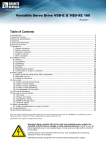
We illustrate connections for these types of LDTs. (There are other
suppliers with compatible LDTs.)
Temposonics II,
RPM or DPM
Interrogate
(+)
9
PS
Common
(+) (–)
7 5 3
1
2
10 8 6 4
(–) (+)
(–)
Frame
GND
Return
"15V dc PS
Balluff
BTL-2-L2 & -2-M2
Interro- Return (–)
Return (+)
gate (–)
2
5
4
(–)
8
3
1
7 (+)
"15V
dc PS
6
Interrogate (+)
PS
Common
Santest
GYRP & GYRG
NC
+15V
dc PS
2
1
Gemco Quick-Stick II
951VP w/PWM Output
B–BLK PS Common
C–RED +15V dc PS
K–GRY + Interrogate
E–BRN –Return*
F–BLU +Return*
A–WHT –Interrogate
G, D, H RS232RXD
J–PUR 2nd PS COM
*951RS has pulse trigger
PS
Common
3
4 (+)
5
7
6 (–)
Return
Return
(+)
(–)
Interrogate
The views are looking at the connector on the LDT head.
LDT Connections (for fabricating your own LDT cable)
Function
Temposonics II
RPM or DPM
Balluff
Santest
BTL-2-L2 & -M2 GYRP/GYRG
Gemco QuickStick 951VP/RS
(+) Return (note 1) 4 – Pink
2 – Gray
pin 5
F – Blue
(–) Return (note 1) 3 – Gray
5 – Green
pin 7
E – Brown
(–) Interrogate
10 – Green
3 – Pink
pin 6
A – White
(+) Interrogate
9 – Yellow
1 – Yellow
pin 4
K – Gray
–15V dc PS
6 – Blue
8 – White
n/a
n/a
PS Common
1 – White
6 – Blue
pin 3
B – Black
+15V dc PS
5 – Red
7 – Brown
pin 1
C – Red
(+) and (–) wires of the same function should be a twisted pair within the cable.
(note 1) We use the term “Return” for gate out, pulse trigger, or square wave (Gemco) and
start/stop (Balluff -M2) LDT signals.
Publication 1746-6.19 March 1998
2–2
Typical Connections to the Interface Module (IFM) Terminal Block
Pin assignments of the IFM terminal block for I/O, power, shield, and
ground connections are as follows: (For example, we show connections
for one axis with a Temposonics LDT and power supply.)
Temposonics II,
RPM or DPM
(+)
9
(+) (–)
7 5 3
10 8 6
(–)
(–)
Drive Output
_
+
"15V
Power Supply
Axis Loop 1
Axis Loop 2
Axis Loop 3
Axis Loop 4
+Ret –Ret +Out Out +Ret –Ret +Out Out +Ret –Ret +Out Out +Ret –Ret +Out Out
1
1
1 Com 2
2
2 Com 3
3
3
Com 4
4
4 Com
0
1
2
3
4
8
12
1
(– ) (C) (+)
2
4
(+)
+Int –Int
1
1
16
17
–V
1F
34
SH
18
SH +Int –Int
2
2
19 20
LDT +V
Com 1F
35 36
SH
–V LDT +V
2F Com 2F
38
SH
+Int –Int SH
3
3
24
–V
LDT
3F Com
42
SH
+V
3F
+Int –Int
4
4
28
–V
4F
46
SH SH
LDT +V
Com 4F
–V
+V
32
33
PS
Earth
Com GND
50 51
Internal Connections:
–V (32) is connected to (34) (38) (42) (46) through fuses that you provide
+V (33) is connected to (36) (40) (44) (48) through fuses that you provide
PS Com (50) is connected to all LDT Com (35) (39) (43) (47)
Earth GND (51) is connected to all SH (18) (19) (22) (23) (26) (27) (30)(31)
Connect the "15V dc power supply to pin 50 (Com), pin 33 (+V), and
pin 32 (–V). Connect pin 51 (GND) to earth ground with 3/8” wire braid
(as short as possible).
Typical Fusing of the Interface Module (IFM) Terminal Block
The Interface Module (IFM) Terminal Block is wired for fusing of
("V) to each LDT. Provide proper fusing (T500L 250V, typical) for
each axis using fuse clips on the IFM terminal block.
Example Connections for Temposonics II Differential Inputs
Use differential inputs when connecting LDTs to the IFM terminal block.
Temposonics II
Function
IFM Terminal Block
Pin #
Function (Axis 1)
Term. #
(+) Interrogate
9
+ Int
16
(–) Interrogate
10
– Int
17
(+) Return
4
+ Ret
0
(–) Return
3
– Ret
1
+ 15V
5
+V 1F
36
–15V
6
–V 1F
34
Comm
1
LDT Com
35
If fabricating your own LDT cable, see connections on previous page.
Publication 1746-6.19 March 1998
2–3
Wiring Example
We present a 1-axis loop with a differential LDT input.
(You must provide power supplies and servo amplifiers.)
"15V Power
Supply for LDTs
(–) (C) (+)
24V Power
Supply
(+) (–)
Axis Loop 1 of 4-axis system
Important: The module’s
analog outputs require an
external amplifier to drive
the valve.
Belden
8761
Connect cable shields of LDT
and drive output to SH terminals
on terminal block (to earth GND).
Servo or
Proportional
Amplifier
Drive Output
0V (internal)
Belden
8761
Grounding exception:
Connect this shield
to internal common.
Piston-type Hydraulic Cylinder and
Linear Displacement Transducer (LDT)
Hydraulic
Configurator
Software on PC
Belden
8770
Connect signal commons and PS commons
to Com terminals, isolated from earth GND.
IFM Terminal Block
Cat. No. 1492-AIFMQS
1747-CP3
Cable
HYDRAULIC
1746-QS
module
SYNCHR AXES
Ret
– +
Int
Valve
Belden
8105
Pwr
Cable 1492ACABLExxxQ
earth ground
Minimizing Interference
from Radiated Electrical
Noise
Important: Signals in this type of control system are very susceptible to
radiated electrical noise. The module is designed to detect loss-of-sensor
and sensor noise conditions for any of the four axes when position values
are lost or corrupted. The Hydraulic Configurator displays these
conditions in the Status word window. The resulting hard or soft stop
depends on how you configured autostop conditions. (See Hydraulic
Configurator, Config word, and click on autostop “Help“).
To minimize interference from radiated electrical noise with correct
shielding and grounding:
• Connect LDT cable shields and drive output cable shields (all
•
•
•
•
•
shields at one end, only) to IFM terminal block SH terminals, and
connect the IFM terminal block GND terminal (51) to earth ground.
Keep LDT signal cables far from motors or proportional amplifiers.
Connect all of the following to earth ground:
– power supply cable shields (one end, only)
– LDT flange, frame, and machine
– I/O chassis
– AC ground
Use shielded twisted pairs for all connections to inputs and outputs.
Run shielded cables only in low-voltage conduit.
Place the SLC-500 processor and I/O chassis in a suitable enclosure.
Publication 1746-6.19 March 1998
2–4
Important: To minimize the adverse effects of ground loops, you must
isolate power supply and signal commons from earth ground as follows:
1. Connect power supply commons to IFM Com terminal (50), and
LDT commons to LDT Com terminals of the IFM terminal block.
Be sure that they are isolated from earth ground.
2. Connect the cable shield of the servo or proportional amplifier
output cable to a zero potential terminal inside the amplifier.
3. Use bond wires that are equal in size to signal wires.
4. When practical, use one power supply to power only your LDTs.
Connecting Outputs
to Output Devices
Note: Follow manufacturer recommendations for shielding the output
cables of the proportional amplifier. Typically, pulse-width modulated
outputs radiate electrical noise originating from the +24V dc power
supply, so isolate the shields of the amplifier output cable to a 0V dc
connection inside the proportional amplifier.
You have a choice of three configurations to match your hydraulics:
• proportional amplifier integrated with a proportional valve
• servo amplifier and variable-volume pump or servo valve
• Allen-Bradley 1305 Drive and hydraulic pump
You may use either of the following output voltage ranges:
• 0-10V dc for an Allen-Bradley 1305 Drive or variable-volume pump
• –10 to +10V dc for a proportional or servo amplifier
If using servo valves, you must convert the module’s output from
voltage to current.
Output Polarity
In most hydraulic systems, the actuator extends (with increasing
LDT counts) when a positive voltage is sent to the output. The
extend direction is defined as the direction that causes the LDT to
return increasing counts moving away from the head.
You can make these selections in the Config word that affect output:
• To generate a positive drive output (0-10V dc) regardless of move
direction, you can select Absolute Mode.
• To extend the actuator by sending a negative voltage to the
output, you can select Reverse Drive Mode.
For additional information on the Configuration word, select that
subject in Help Topics.
Publication 1746-6.19 March 1998
2–5
Checking Out the
Wiring and Grounding
Repeat this procedure to check out each of the four axis loops
connected to the IFM terminal block.
ATTENTION: Be sure to remove all power to the SLC processor,
LDT, valve and pump beforehand.
1. Disconnect the LDT connector at the head end.
2. Disconnect the connector to the IFM terminal block.
3. Turn ON the power supplies for the LDT and SLC processor, and
check the LDT connector and IFM terminal block for:
• +15V dc
• PS common
• –15V dc
4. Observe that the module’s fault LED indicates Green.
5. Verify continuity between IFM COM terminal (50) and each of:
• shield of the amplifier output cable to the valve
• output common on "15V dc PS that powers the LDT
• (–) terminal on +24V dc PS that powers the proportional amplifier
6. Verify NO continuity between drive output commons connected to
IFM terminals 3, 7, 11, 15 and earth ground.
7. To minimize ground loops, verify that all cable shields are grounded
(at one end, only) to SH terminals of the IFM terminal block, and
that GND terminal (51) of the IFM is connected to earth ground.
Setting Up the Hydraulics
1. Design for adequate pressure and volume. Hydraulic systems
must have enough pressure and fluid volume (accumulator) to move the
desired load the commanded distance and speed. Inadequate pressure
or volume will cause the axis to lag the target position as the controller
attempts to move the axis faster than the system can move. Consider
monitoring system pressure or providing a low-limit (approx. 80%)
pressure switch.
2. Avoid flexible hose. Use no flexible hose between the valve and
the cylinder being controlled. Flexible hose will swell and contract
as the valve opens and closes, causing oscillation and loss of control.
3. Mount valve and cylinder in correct orientation. To avoid
problems from entrapped air, mount the valve directly to the cylinder
and positioned above it. Mount pressure sensors beneath the cylinder.
4. Use linear valves with minimal overlap. If using proportional
valves, they should have less than 3% overlap and a linear (not
curvilinear) response. Nonlinear valves or valves with excessive
(20%) overlap may cause oscillation or hunting. We recommend
using servo valves or servo-quality proportional valves.
Publication 1746-6.19 March 1998
2–6
5. Avoid valves with a slow response (less than 60 Hz). Valves with
slow response cause the module to overcompensate for disturbances in
the motion of the system. Since the system does not respond immediately
to the control signal, the module continues to increase the drive signal.
By the time the system begins to respond to the error, the control signal
has become too large and the system overshoots. The module then
attempts to control in the opposite direction, but again overshoots. These
valves can cause the system to oscillate around the set point as the
module overshoots first in one direction, then the other.
Regarding the Interface
Module Terminal Block
(Cat. No. 1492-AIFMQS)
and Cable
We recommend that you use the Interface Module (IFM) terminal
block (Cat. No. 1492-AIFMQS) to connect module I/O and power.
It facilitates power supply, shield, and fuse connections.
It is required for CE certification.
The pre-wired cable that connects the IFM terminal block to the
module is available in standard sizes as indicated by its part number,
1492-ACABLExxxQ, where xxx indicates the length in meters:
length:
xxx:
0.5 m
005
1.0 m
010
2.5 m
025
Important: Because the sytem was certified with a shorter cable,
you must re-certify the system if using the 2.5 m cable.
Publication 1492-5.1 describes the IFM terminal block and cables.
For information on the entire line of Allen-Bradley Interface
Modules and associated cables for wiring analog systems, refer to
publication 1492-2.15.
Publication 1746-6.19 March 1998
Chapter
3
Setting Up Your PC for the
Hydraulic Configurator
Chapter Objectives
This chapter helps you do the following:
• Obtain the Hydraulic Configurator from the Internet
• Set up communication between your PC and the module
Obtaining the Hydraulic
Configurator from the
Internet
You can download the Hydraulic Configurator from our website to
your PC. (You can also download ladder logic and transfer it to your
SLC processor, but we cover that in chapter 6.)
System requirements for the Hydraulic Configurator are:
Windows ’95 series A or B and 4M available disk space.
To Access Our Website:
Access the Allen-Bradley website (and 1746-QS software) at:
The Hydraulic Configurator is stored there as a self-extracting
Winzip executable.
To Load the Hydraulic Configurator:
1. Download the Hydraulic Configurator (1746-QS.EXE) onto your
hard drive.
2. Run 1746-QS.EXE. The Winzip self-extractor will ask you
where you want to store the Hydraulic Configurator.
3. Launch it using the file, QsCfg.exe.
4. Set up a shortcut (optional).
Publication 1746-6.19 March 1998
3–2
Setting Up Communication
Between PC and Module
You must establish communication between Hydraulic Configurator
software on your PC and the module.
1. Connect your PC to the module with Allen-Bradley cable (cat. no.
1747-CP3): one end to a serial port on your PC such as COM1, the
other end to the 9-pin D-shell connector on the module.
Windows ’95 provides a virtual connection to the serial port without
any intervention unless that port is already used by another application.
Important: You may run RSLogix500 and Hydraulic Configurator
concurrently on your PC if you have both COM1 and COM2
available. If only one serial port is available, you may use the
Communication Interface Card (1784-KTx) for the connection
between PC and SLC processor.
2. Open the Hydraulic Configurator by running QsCfg.exe.
The main screen appears.
If you also get the message “No Motion Controller Detected,” then:
– check the1747-CP3 cable connection between PC and module
– match the software/hardware COM ports (step 3.)
Otherwise, go to step 4.
3. Set the Hydraulic Configurator COM port to match your PC.
To do this, click Tools on the toolbar, then Monitor Options from
the menu. Enter the COM port number you used for your PC cable
connection to the module in step 1.
4. To verify communication with the module, observe that the Com:
window (screen bottom left) displays “Online“.
Important: You can run the Hydraulic Configurator offline to view
plots, stored data files, and access Help screens.
Publication 1746-6.19 March 1998
Chapter
4
Tuning an Axis with the
Hydraulic Configurator
Chapter Objectives
We cover these topics:
•
•
•
•
•
•
•
Before You Begin
Before You Begin
Finding the Value of the Null Drive
Moving the Axis to Set Offset, Scale, Extend and Retract Limits
Getting Ready to Tune the Axes
Tuning Each Axis
Finding the Value of the Dead Band Eliminator
Saving Parameters
ATTENTION: Great care must be taken to avoid accidents when
starting the module for the first time. The most common accident is
a runaway, where the module tries to move the axis to a position
beyond the physical limits, or in the wrong direction while in
closed-loop control.
When the module is first turned on, parameters are set to default
values. You must change these parameters (with the Hydraulic
Configurator) to operate the module in your application.
ATTENTION: Do not attempt to operate the module in closed-loop
mode until EXTEND and RETRACT limits have been determined
and initialized in the module using the Hydraulic Configurator.
Before starting, be sure that:
1. Hydraulic Configurator is communicating with the module
2. Important: You have identified the type of LDT output. To Do this:
– Double-click the Config word in the screen’s PARAMETER section.
– Click the transducer type that matches your LDT.
– Disable simulate mode.
Do this by removing the nfrom its check box in the Config word.
– Leave the other selections at default.
3. LDTs are connected and powered up
Finding the Value
of the Null Drive
The Null Drive compensates for axis drift.
This procedure requires operating the module in open-loop mode
with drive outputs connected to the amplifier. In this procedure,
you will increase the drive output until the axis stops drifting. Then
you will initialize that value in the module with an “N” command.
Publication 1746-6.19 March 1998
4–2
1.
2.
3.
4.
5.
6.
7.
8.
Moving the Axis to Set
Scale, Offset, Extend,
and Retract Limits
Turn off the power to the module.
Connect the axis drive output to the amplifier.
Turn the power back on.
Turn on the hydraulics.
If the axis drifts, go to step 5.
If not, you are done. Go to the next procedure, Moving the Axis.
Find the Null Drive value to stop axis drift:
a) Estimate a drive output (mV) required to hold zero motion.
b) Command the module to output that value with the “O“ command:
– Select axis and enter value into COMMAND VALUE number field.
– From Command in the CommandBar, click the “O“ command.
c) Repeat until the value produces no drift. This is the Null Drive
Zero the open-loop output with the “K” (Kill) command. To do this:
– Click [K] in the ToolBar.
Important: The axis will resume its initial drift until you do step 7.
Command the module to output the Null Drive with “N” command.
– Enter Null Drive into COMMAND VALUE number field.
– From Command in the CommandBar, click the “N“ command.
If drift persists, adjust Null Drive with “N” commands (as in step 7).
By moving the axis, you will calibrate these configuration parameters
with the Hydraulic Configurator:
• Scale
• Offset
• Extend and Retract Limits
We give you a preferred and an alternate procedure based on whether
the drive output is disconnected from or connected to the module:
If:
Then:
You have a diddle box*
to move the axis
Use the preferred procedure
with the drive output disconnected
Use the alternate open-loop procedure
You do Not have a diddle box
with the drive output connected
* a control box that can electrically drive the valve amplifier
Procedure to Set Scale and Offset with Drive Output Disconnected
With the axis drive output disconnected and the LDT on, you will move
the axis with a diddle box (or manually) to two known machine positions
(typically the extend and retract limits). There you will use the Hydraulic
Configurator “Scale/Offset Calibration” feature to enter ACTUAL
POSITION and COUNTS values.
Important: When moving to axis limits, be sure to leave space for safety.
Remember that extend is the direction that returns increasing LDT COUNTS.
Publication 1746-6.19 March 1998
4–3
1.
2.
3.
4.
5.
Turn off the power to the module.
Disconnect the axis drive output to the amplifier.
Turn the power back on.
Turn on the hydraulics.
Move the axis to the first position with the diddle box.
It doesn’t matter whether the first position is an extend or retract.
6. In the Scale/Offset Calibration window (from Tools in command bar):
a) Enter the desired position value into the Actual Position field for
the First Position. (For example, –4000)
b) In corresponding First Position Counts field, click “Use Current”.
7. Move the axis from the first position to the second.
8. In the Scale/Offset Calibration window (from Tools in CommandBar):
a) Enter the desired position value in the Actual Position field for the
Second Position . (For example, 40,000)
b) In corresponding Second Position Counts field, click “Use Current”.
The New Parameters area of the window will show the calculated values
for the Config word, Scale, and offset. (Set extend/retract limits later.)
9. Confirm that the displayed New Parameters (step 8) are valid. Then,
a) Click “Apply” to enter the values into configuration parameter words.
b) Click “Done” to close the editor window.
Important: You must set the EXTEND and RETRACT LIMITS after
setting the scale and offset. The Scale/Offset Calibration tool will
re-calculate any existing EXTEND and RETRACT LIMITS automatically
when you use it to set a scale and offset.
10.For each axis, enter the desired end-point values for the EXTEND
and RETRACT LIMITS in the screen’s PARAMETER section.
Enter them in the same engineering units as used in steps 6 and 8.
11. Transfer the parameters to the module using the “P” Command.
12.Repeat this procedure for each axis in use.
Alternate Open-loop Procedure to Set Scale and Offset
You will move the axis with the module in open-loop mode to two
known machine positions (typically the extend and retract limits).
There you will use the Hydraulic Configurator “Scale/Offset
Calibration” feature to enter ACTUAL POSITION and COUNTS values.
ATTENTION:
A. Drive outputs will be connected to the amplifier.
B. Open-loop operation will ignore all limits.
Be prepared to instantly remove drive power.
C. To avoid surprises, read the entire procedure before starting.
1. Turn off the power to the module.
2. Connect the axis drive output to the amplifier.
Publication 1746-6.19 March 1998
4–4
3. Turn the power back on.
4. Turn on the hydraulics.
If the axis drifts, go back to the Null Drive procedure.
If not, go to step 5.
5. To move the axis to the first position (either extend or retract).
a) Estimate drive output (mV) that would generate a slow safe speed.
Enter it into the COMMAND VALUE number field.
Note: In open-loop mode, this field sets the module output.
In closed-loop mode, this field sets the commanded position.
b) Command the module to output that value with the “O“ command.
The axis should start to move.
6. To stop axis motion:
a) Zero the COMMAND VALUE number field.
b) Command the module to zero its output with an “O” command.
7. In Scale/Offset Calibration window (from Tools in CommandBar):
a) Enter the desired position value in the Actual Position field for
the First Position . (For example, 40,000)
b) In corresponding Counts field, click “Use Current”.
8. To move the axis to the second position:
a) Command the module to output a negative value (such as –200)
with the “O” command (as with step 5b).
The axis should start to retract. If not, verify that the value is (–).
9. To stop axis motion:
a) Zero the COMMAND VALUE number field.
b) Command the module to zero its output with an “O” command.
10. In the Scale/Offset Calibration window (from Tools in command bar):
a) Enter the desired position value in the Actual Position field for the
Second Position . (For example, –4000)
b) In corresponding Counts field, click “Use Current”.
The New Parameters area of the window will show the calculated values
for the Config word, Scale, and offset. (Set extend/retract limits later.)
11. Confirm that the displayed New Parameters (step 10) are valid. Then,
a) Click “Apply” to enter the values into configuration parameter words.
b) Click “Done” to close the editor window.
Important: You must set the EXTEND and RETRACT LIMITS after
setting the scale and offset. The Scale/Offset Calibration tool will
re-calculate any existing EXTEND and RETRACT LIMITS automatically
when you use it to set a scale and offset.
12.For each axis, enter the desired end-point values for the EXTEND
and RETRACT LIMITS in the screen’s PARAMETER section.
Enter them in the same engineering units as used in steps 7 and 10.
13. Initialize (activate) axis parameters with the “P” Command.
14.Repeat this procedure for each axis in use.
Publication 1746-6.19 March 1998
4–5
Getting Ready to
Tune the Axes
Once you have set scale, offset, and extend/retract limits in open-loop
mode, you can now use the Hydraulic Configurator to tune the axis
using closed-loop move commands and axis plots. We suggest that you:
1. Leave un-entered configurations parameters at default, except for:
– Auto Stop to 000E0 (hard stop, only for LDT faults)
2. If not done already, initialize the axes with the “P” command.
3. Store two 6-word motion commands in the Stored Command Editor:
– Mode word = 00000
(This sets integrator to Always Active and accel/decel to slow ramp.)
– SPEED, ACCEL, and DECEL values at 20% of typical machine move
(For safety, start slow and increase SPEED gradually.)
– COMMAND VALUEs to desired end positions for the axis to tune
– Zero all six command words of the axes not to be tuned
4. Set the plot clock (in even-numbered seconds, 20 max) to longer
than you expect for the axis to run “tuning” moves.
5. ATTENTION: Highlight the axis you want to move before moving
the axis back and forth using stored commands [1] and [2].
Unexpected motion could occur if the wrong axis is highlighted.
6. Open the status bits window (Ctrl-B), and check the STATUS word
for errors while the axis is moving.
7. View captured axis plots (click [∩ ] in the ToolBar).
Observe the Sum-Error2 value displayed in the window.
Tuning Each Axis
‘There is no substitute for experience when tuning an axis. This
section offers some guidelines, tips, and suggestions for tuning your
system. While helpful for many systems, they may not be the best
for a particular system. We help you with:
• General Procedure for Tuning an Axis
• Adjusting Command-word Speed and Acceleration values
• Adjusting Feedforward Parameters
• Using Acceleration Feedforwards
• Adjusting PID Gains
General Procedure for Tuning an Axis
Use this generalized procedure with the Hydraulic Configurator.
• Move the axis using stored commands [1] and [2].
• Observe the axis plot for each move.
• Adjust one configuration parameter at a time in the order given.
1. Observe plots of axis moves between the two positions that you
set up with stored commands in the previous section, Getting
Ready. Observe following error, overshoots, and oscillations.
For adjusting command values and configuration parameters, refer to
Adjusting Command-word Speed and Acceleration Values, page 4-7.
Publication 1746-6.19 March 1998
4–6
2. The Following Error will probably vary as indicated by diverging plots
of target and actual speeds during acceleration or deceleration.
Target Speed
(pink)
Actual Speed
(dark blue)
Following Error
3. To achieve a nearly constant steady-state Following Error, increase
the PROPORTIONAL GAIN until the plots of target and actual speeds
become parallel during acceleration or deceleration.
4. To minimize the Following Error, use the auto Adjust Feedforward
“F” command. With each “F” command, the module boosts
(prescales) the drive output by increasing the FEEDFORWARD term.
This brings the plots of target and actual positions to coincide.
Target Position
(powder blue)
Actual Position
(red)
Following Error
For additional information, refer to Feedforward Parameters, below.
5. For critical tuning, adjust the ACCELERATION FEEDFORWARD term.
To do this, observe the Sum-Error2 value found in the window on the
plot screen. Repeat axis moves with adjustments until Sum-Error2
value reaches a minimum. Too much ACCELERATION
FEEDFORWARD will increase the Sum-Error2 value.
Important: Critical tuning may increase pressure spikes. If the
axis load is too large, consider lowering your expectations of
machine performance and use smaller accel/decel values in the
motion command. Using the S-curve feature (Command Mode)
is another alternative.
For additional information on Acceleration Feedforward, refer to
Using Acceleration Feedforward, below.
6. For end-point stability, adjust the PROPORTIONAL GAIN (and
INTEGRAL GAIN) to minimize the end-point position error by either
of two ways. Adjust P and/or I until the:
– end position oscillates. Then back down to 75% of P.
– Sum-Error2 value no longer decreases with each adjustment.
Remember to enter an IN POSITION value in the Config word to
monitor end-position stability.
Publication 1746-6.19 March 1998
4–7
7. If moving a relatively large mass with a relatively small hydraulic
cylinder, first investigate the affect of:
a) Integrator Mode selection in the Command-mode word:
active always, for accel/decels, in position, or never.
b) Integrator Limit selection in the Config word:
20% for a typical hydraulic system, 80% for a difficult system.
Also, see step 6 for using INTEGRAL GAIN to help minimize the
end-point position error.
For additional information on PID Gains, refer to that topic, below.
Adjusting Command-word Speed and Acceleration Values
Increase the SPEED and ACCELERATION command words gradually
while making long moves. Use Hydraulic Configurator to plot the
moves and look for following errors, overshoot, or oscillations.
Eventually, when the SPEED and ACCELERATIONS are too high, the
moves will cause an error on the axis.
If an overdrive error occurs, there is not enough drive capacity to drive
the axis at the requested SPEED. Should this occur, reduce the SPEED.
If excess Following Error occurs, the appropriate FEEDFORWARD
configuration parameter must be adjusted for extend and retract moves.
If excess Following Error persists, ACCEL and DECEL ramps may be too
steep for your system response. You can reduce their values, or increase
the ACCEL FEEDFORWARD term.
Also remember that you can specify either the time or the distance in
which the ACCELERATION or DECELERATION must occur.
After correcting the problem of excess Following Error, keep moving the
axis back and forth with increasing SPEED values until you reach desired
speed. Should the system seem a little sloppy, try increasing the
PROPORTIONAL GAIN until the axis moves with a steady state
FOLLOWING ERROR (as observed by axis plot) and stops at the end point
with minimum in-position error. Remember: the parameters are not
updated in the module until you issue the “P” command.
Adjusting Feedforward Parameters
In many hydraulic systems the feedforward parameters (EXTEND
FEEDFORWARD and RETRACT FEEDFORWARD) are the most
important parameters for position tracking during a move.
Use the auto Feedforward Adjust command “F” to minimize the
FOLLOWING ERROR. Refer to General Tuning Procedure, step 2.
For move information, refer to these parameters in the Help Topics.
Publication 1746-6.19 March 1998
4–8
Important: When tuning the Feedforward term with command “F”,
plot sequential axis moves and compare plots of target position and
actual position until the two plots coincide.
Another way to adjust these parameters is to set the DIFFERENTIAL
GAIN and INTEGRAL GAIN to zero and the PROPORTIONAL GAIN
to a small value (between 1 and 5), then make long slow moves in
both directions.
Adjust the EXT FEEDFORWARD and RET FEEDFORWARD until the
axis tracks within 10% in both directions. In hydraulic systems, the
EXTEND and RETRACT FEEDFORWARD terms typically differ by
the ratio of the extend and retract piston areas.
Alternately, you can find the appropriate value for the FEEDFORWARD
terms by making moves with the axis at a SPEED of 1,000. The
amount of output drive required to maintain this SPEED is the correct
value for the FEEDFORWARD parameter.
Using Acceleration Feedforwards
The ACCELERATION FEEDFORWARD terms are particularly useful for
axes which move large masses with relatively small cylinders. This
combination delays the start of movement, and the ACCELERATION
FEEDFORWARD terms can help compensate for this delay.
ACCELERATION FEEDFORWARDS are easiest to adjust with the PID
gains set low. After commanding a move, plot it using Hydraulic
Configurator and look for a following error during the acceleration.
Increase the ACCELERATION FEEDFORWARD until the error is
minimized. For large masses the ACCELERATION FEEDFORWARD can
be in the tens of thousands.
Important: When tuning acceleration feedforward terms, you can
plot multiple axis moves and observe the Sum-Error2 value found in
the window on the plot screen. Repeat axis moves and adjust this
term until the Sum-Error2 value reaches a minimum.
Adjusting P-I-D Gains
PROPORTIONAL GAIN affects the responsiveness of the system.
Low gains make the system sluggish and unresponsive. Gains that
are too high make the axis oscillate or vibrate. You can adjust the
PROPORTIONAL GAIN by slowly increasing it and moving the axis.
When you see a tendency to oscillate as the axis moves or stops,
reduce the gain by 10 to 30 percent.
Publication 1746-6.19 March 1998
4–9
It is usually desirable to have some INTEGRAL GAIN (5 to 50 counts)
to help compensate for valve null drift or changes in system dynamics.
Some systems may require larger INTEGRAL GAIN, in particular if
they are moving a large mass or are nonlinear. Too much INTEGRAL
GAIN will cause oscillations. On the other hand, some hydraulic
systems do not require INTEGRAL GAIN.
DIFFERENTIAL GAIN is used mainly on systems which have a
tendency to oscillate. This happens when heavy loads are moved
with relatively small cylinders. DIFFERENTIAL GAIN will tend to
dampen out oscillations and help the axis track during acceleration
and deceleration. If you use DIFFERENTIAL GAIN, you may be able
to increase the PROPORTIONAL GAIN somewhat without causing the
system to oscillate.
A disadvantage to DIFFERENTIAL GAIN is that it amplifies position
measurement noise which can cause the system to chatter or
oscillate if the gain is too high or there is too much noise.
Finding the Value of the
Dead Band Eliminator
The DEAD BAND ELIMINATOR compensates for valve overlap.
Typically it is required if the valve has relatively:
• large overlap (up to 20%)
• slow speed (less than 40 Hz)
• large capacity for its application
(For a description of how Dead Band Eliminator affects the system,
refer that subject under Hydraulic Configurator Help Topics.)
Important: Use this procedure only if your valve needs the DEAD
BAND ELIMINATOR. If not, go to the next section, Saving Parameters.
This procedure requires operating the module in open-loop mode with
drive outputs connected to the amplifier. In this procedure, you will
increase the drive output until the axis just moves in one direction, then
in the other.
1. Select the axis and enter a small positive value (such as 200 mV)
in the COMMAND VALUE number field.
2. Issue the open-loop output command “O”.
3. Look for axis motion.
4. Important: If necessary, be prepared to stop axis motion. To stop:
– Enter zero in the COMMAND VALUE number field.
– Issue the open-loop output command “O”.
5. Slowly increase the value that you entered in the COMMAND VALUE
number field, and repeat steps 2 and 3 until the axis just starts to move.
Important: Observe if the axis moved in the intended direction.
If in the wrong direction, check drive wiring polarity and hydraulic
plumbing before reversing the drive mode in the Config word.
Publication 1746-6.19 March 1998
4–10
6. Back down the value below no motion. Write down this valve.
7. Repeat steps 1-6 with negative values for opposite direction.
8. Determine DEAD BAND ELIMINATOR value. It is the larger of the
values from step 6, regardless of sign (").
9. Enter the value of the DEAD BAND ELIMINATOR in the number
field in the Parameter section of the main screen.
10.Transfer the parameter to the module using the “P” Command.
Saving Parameters
At any time during tuning, you can save configuration parameters:
• For PC backup, save the file of configuration parameters from the
Hydraulic Configurator with the “Save-as” function.
• Store them in integer (N) files of the SLC processor to insure that
the ladder program matches the configuration parameters, issue a
ladder logic command to copy the M1 file of configuration
parameters from the module into SLC processor integer (N) files.
For ladder logic examples, refer to chapter 5.
Publication 1746-6.19 March 1998
Chapter
5
Using Ladder Logic
Chapter Objectives
This chapter covers:
• Obtaining sample ladder program from the Internet
• Configuring your SLC processor, off-line
• Using the sample ladder program, RSExampl.RSS, to:
– copy configuration parameters to the SLC processor
– copy configuration parameters to the module
– operate axis movement automatically
– jog the axis
– respond to loss or restoration of hydraulic power
– run multiple synchronized axes
Obtaining Sample Ladder
Program from the Internet
You can obtain sample ladder logic from the Allen-Bradley website
on the Internet and download it to your PC as an executable file.
To Access the Internet:
1. Access the Allen-Bradley website (and module software logic) at:
2. The sample ladder program (130 Kbyte) is in the same file as the
Hydraulic Configurator (2.9Mbyte).
3. Download the Hydraulic Configurator and ladder program to your PC.
4. Move the sample program into the subdirectory on your hard drive
where your programming software looks for files.
For example, with RSLogix500: C:\RSI\Logix500\QSEXAMPL.RSS.
Configuring Your
SLC Processor, Off-line
This procedure uses RSLogix500 version 2.0 or later. For other types of
programming software, the procedure and/or prompts may vary.
You must modify the I/O configuration to match your system layout and
change associated addresses, offline.
1. Open file QSEXAMPL.RSS from the file pull-down window.
2. Select the I/O Configuration icon and launch it. Then select:
A. Processor type (ladder sample is SLC 5/04).
B. Module slot number (ladder sample is slot 2 in 4-slot chassis).
C. Module ID is 13627 entered under “Other”.
3. The sample ladder logic creates M0/M1 files at 64 words each.
If you move the module to another slot, be sure to retain the files.
4. Search and replace all addresses that must be changed.
5. Save the file as a new file to preserve the original file for backup.
Publication 1746-6.19 March 1998
5–2
Using the Sample Ladder
Program
Consider creating a bit and data address table for your own applicaion.
Data and bit addresses associated with the sample program are:
Address:
Description:
N7:0
current state of axis 1, programmed automatic motion
N7:1
current state of axis 2, programmed automatic motion
N7:4
next state of axis 1, programmed automatic motion
N7:5
next state of axis 2, programmed automatic motion
N11
M-file initialization parameters
N12:0-5
axis 1 advance profile, programmed automatic motion
N12:6-11
axis 2 advance profile, programmed automatic motion
N12:12-17
axis 1 retract profile, programmed automatic motion
N12:18-23
axis 2 retract profile, programmed automatic motion
N12:24-29
axis 1 advance profile for jog
N121:30-35
axis 1 retract profile for jog
B3:0/0
copy M file from N11 into module and initialize axis 1 and 2
B3:0/1
copy M file from module into N11
B3:0/3
jog advance
B3:0/4
jog retract
B3:0/7
enter programming for automatic motion
Load the ladder file into the SLC processor.
Important: You can run the sample ladder program from the desktop
using pre-programmed configuration parameters in file N11 without
LDT or drive output connections to the module because the Simulate bit
is set by default in each axis Config word in the sample program.
ATTENTION: To guard against equipment damage or personal injury,
do NOT attempt to operate the module outside of simulate mode
without first initializing valid configuration parameters in the module.
If you have already initialized the module with valid configuration
parameters that suit your machine, you should copy them from the
module into the N11 file. (Refer to Copy Configuration Parameters to
the SLC Processor, next.)
If you have NOT initialized the module with valid configuration
parameters, copy the N file of the sample program to the module to
initialize axis 1 and 2 with pre-programmed configuration parameters
(Refer to Copy Configuration Parameters to the Module, next.)
Publication 1746-6.19 March 1998
5–3
Copy Configuration Parameters to the SLC Processor
|
INITIALIZE GET from QS Module
| Enable this rung to copy configuration parameters to the SLC N file
|
| after you change them with the Hydraulic Configurator.
|
|
|
| Set ON to read
|
| parameters
|
| after tuning
Parameters for Axis 1
|
| GET_PARAMETERS
CONFIG1
|
|
B3:0
+COP–––––––––––––––+
|
|–––] [–––––––––––––––––––––––––––––––––––––––––+–+COPY FILE
+–+–|
|
1
| |Source
#M1:2.0| | |
|
| |Dest
#N11:0| | |
|
| |Length
64| | |
|
| +––––––––––––––––––+ | |
|
|
| |
|
|
Set ON to read
| |
|
|
parameters
| |
|
|
after tuning
| |
|
|
GET_PARAMETERS
| |
|
|
B3:0
| |
|
+––––––––––(U)–––––––––+ |
|
1
|
Copy Configuration Parameters to the Module
This rung copies configuration parameters from SLC N11 file to the
module’s M0 file and issues the “P” command for axis 1 and 2.
The “P” command is the decimal value “80” that is moved to output
image Command words O:2.5 (axis 1) and O:2.13 (axis 2).
Important: Configuration parameters copied to the module’s M0
file are not initialized (activated) until the “P” command is issued.
Important: This rung will overwrite configuration parameters
currently stored in the module. If you want to retain configuration
parameters stored in the module, be sure that you have copied them to
the N11 file (previous section) before activating this rung.
| Set ON to
|
| initialize the
|
| QS module
|
| INITIALIZE
M0_PARAMETER_DATA
|
|
B3:0
+COP–––––––––––––––+
|
|–––] [–––––––––––––––––––––––––––––––––––––––––+–+COPY FILE
+–+–|
|
0
| |Source
#N:11.0| | |
|
| |Dest
#M0:2.0| | |
|
| |Length
64| | |
|
| +––––––––––––––––––+ | |
|
|
| |
|
| AXIS1_COMMAND
| |
|
| +MOV–––––––––––––––+ | |
|
+–+MOVE FILE
+–+ |
|
| |Source
80 | | |
|
| |
80<| | |
|
| |Dest
#O:2.5 | | |
|
| |
71<| | |
|
| +––––––––––––––––––+ | |
|
|
| |
|
| AXIS2_COMMAND
| |
|
| +MOV–––––––––––––––+ | |
|
+–+MOVE FILE
+–+ |
|
| |Source
80 | | |
|
| |
80<| | |
|
| |Dest
#O:2.13 | | |
|
| |
71<| | |
|
| +––––––––––––––––––+ | |
|
|
| |
|
|
Set ON to
| |
|
|
initialize the
| |
|
|
the QS module
| |
|
|
INITIALIZE
| |
|
|
B3:0
| |
|
+––––––––––(U)–––––––––+ |
|
|
0
| |
|
|
| |
|
|
Last command
| |
|
|
has NOT been
| |
|
|
acknowledged
| |
|
|
AXIS_WAIT_ACK
| |
|
|
B13:0
| |
|
+––––––––––(L)–––––––––+ |
|
0
|
Publication 1746-6.19 March 1998
5–4
Back and Forth Motion with State-machine Logic
(Programming for Automatic Operation)
This ladder logic example moves axes 1 and 2 back and forth with
Go “G” commands. Each move has its own set of motion profile
words (mode, accel, decel, speed, and position).
The example is a state machine with four automatic states:
State:
0
1
2
3
Description:
No motion. Used when automatic mode is not enabled
Moves axis 1 and 2 independently
Uses profile command words N12:0-5 (axis 1) and N12:12-17 (axis 2)
Synchronizes axis 1 and 2 to reach the end point at the same time
Uses profile command words N12:6-11 (axis 1) and N12:18-23 (axis 2)
Pauses five seconds, then returns to state 1.
Error detection and recovery logic is application dependent, and
should include (for each axis) recovery from module-detected errors
and axis timeouts.
The mode words in these profile commands put the module into
simulate mode, which means it is isolated from LDT inputs and
output drive. It allows for axis-position update and axis plotting.
You cannot be jogging when you attempt to enter automatic mode, and
you cannot be in automatic mode when attempting a jog.
Important: If you intend to use this sample program on a live machine
(module NOT in simulate mode), be sure that you have:
– stored valid motion profiles in N12 files
– initialized the module with valid configuration parameters such as
axis limits, scale, offset, and feedforwards
Assuming that axes are initialized, the setting of bit B3:0/7 simulates
an auto operation switch that starts the state machine in state 1.
| To run this example, set HYDRAULICS OK bit in the data table.
|
| Then set the AUTO_SS bit.
|
|
|
|
Valve drive power
|
| Imitates
and pumps are ON,
|
| Operator
electronic servo
Run state |
| Auto Mode valve is enabled,
Axis has received
machine
|
| select SW blocking valves open valid “P” command
Axis is jogging
example
|
| AUTO_SS
HYDRAULICS_OK
AXIS1_INITIALIZED
AXIS JOGGING
AUTO_MODE |
| B3:0
B3:0
I:2
B13:3
B3:0
|
|–––] [–––––––––] [–––––––––––––––––––] [–––––––––––––––––––]/[––––––––––––( )––––|
|
7
2
70
0
14
|
|
|
| Set the state machine to state 1 for all axes when entering auto mode.
|
| This fill command initializes all four axes.
|
|
|
| Run state
|
| machine
|
| example
One Shot
|
| AUTO_MODE
AUTO_MODE_OS
AXIS1_NEXT_STATE
|
|
B3:0
B3:0
+FLL–––––––––––––––+ |
|–––] [––––––––––––––[OSR]––––––––––––––––––––––––––––––––––––+FILE FILL
+–|
|
14
15
|Source
1 | |
|
|Dest
#N7:4 | |
|
|Length
4 | |
|
+––––––––––––––––––+ |
Publication 1746-6.19 March 1998
5–5
|
|
| Reset the state machine for all axes if not in auto mode.
|
| In state 0, the auto mode state machine does not write to the module’s I/O.
|
|
|
| Run state
|
| machine
|
| example
|
| AUTO_MODE
AXIS1_NEXT_STATE
|
|
B3:0
+FLL–––––––––––––––+ |
|–––]/[–––––––––––––––––––––––––––––––––––––––––––––––––––––––+FILE FILL
+–|
|
14
|Source
0 | |
|
|Dest
#N7:4 | |
|
|Length
4 | |
|
+––––––––––––––––––+ |
|
|
| Copy next state to state machine.
|
| This technique avoids race conditions.
|
|
AXIS1_NEXT_STATE
|
|
+COP–––––––––––––––+ |
|–––––––––––––––––––––––––––––––––––––––––––––––––––––––––––––+COPY FILE
+–|
|
|Source
#N7:4 | |
|
|Dest
#N7:0 | |
|
|Length
4 | |
|
+––––––––––––––––––+ |
| AXIS 1 and 2 STATE 1
|
|
|
| Use motion profile words (mode, accel, decel, speed, and command) stored in
|
| N12:0-5 (axis 1) and N12:12-17 (axis 2).
|
| Wait for IN-POSITION bit to go high. Then set NEXT STATE to 2.
|
|
|
|
Oneshot
|
| AXIS1_STATE
storage Bit
AXIS1_MODE
|
| +EQU–––––––––––––––+
B3:1
+COP–––––––––––––––+
|
|––+EQUAL
+––+–––[OSR]––––––––––––––––––––––+–+COPY FILE
+–+–+–|
| |Source A
N7:0 | |
0
| |Source
#N:12.0| | | |
| |
3<| |
| |Dest
#O:2.0| | | |
| |Source B
1 | |
| |Length
6| | | |
| |
1<| |
| +––––––––––––––––––+ | | |
| +––––––––––––––––––+ |
|
| | |
|
|
| AXIS2_MODE
| | |
|
|
| +COP–––––––––––––––+ | | |
|
|
+–+COPY FILE
+–+ | |
|
|
| |Source
#N12:12| | | |
|
|
| |Dest
#O2:8| | | |
|
|
| |Length
6| | | |
|
|
| +––––––––––––––––––+ | | |
|
|
|
| | |
|
|
|
Last command
| | |
|
|
|
has not been
| | |
|
|
|
acknowledged
| | |
|
|
|
AXIS_WAIT_ACK
| | |
|
|
|
B13:0
| | |
|
|
+––––––––(L)–––––––––––+ | |
|
|
0
| |
|
| Last command
ACTUAL POSITION is
| |
|
| has not been
within IN POSITION
| |
|
| acknowledged
units of COMMAND
| |
|
| AXIS_wAIT_ACK POSITION
AXIS1_NEXT STATE
| |
|
|
B13:0
I/2
+–+MOV–––––––––––––––+ | |
|
+–––––––]/[––––––––––] [–––––––––+–+MOVE FILE
+–+ |
|
0
64
| |Source
2 | | |
|
| |
2<| | |
|
| |Dest
N7:4 | | |
|
| |
3<| | |
|
| +––––––––––––––––––+ | |
|
|
| |
|
| AXIS2_NEXT STATE
| |
|
| +MOV–––––––––––––––+ | |
|
+–+MOVE FILE
+–+ |
|
|Source
2 |
|
|
|
2<|
|
|
|Dest
N7:5 |
|
|
|
3<|
|
|
+––––––––––––––––––+
|
|
|
Publication 1746-6.19 March 1998
5–6
| AXIS 1 and 2 STATE 2
|
|
|
| Use motion profile words (mode, accel, decel, speed, and command) stored in
|
| N12:6-11 (axis 1) and N12:18-23 (axis 2).
|
| Wait for IN-POSITION bit to go high. Then set NEXT STATE to 3.
|
|
|
|
Oneshot
|
| AXIS1_STATE
storage Bit
AXIS1_MODE
|
| +EQU–––––––––––––––+
B3:1
+COP–––––––––––––––+
|
|––+EQUAL
+––+–––[OSR]––––––––––––––––––––––+–+COPY FILE
+–+–+–|
| |Source A
N7:0 | |
12
| |Source
#N:12.6| | | |
| |
3<| |
| |Dest
#O:2.0| | | |
| |Source B
2 | |
| |Length
6| | | |
| |
2<| |
| +––––––––––––––––––+ | | |
| +––––––––––––––––––+ |
|
| | |
|
|
| AXIS2_MODE
| | |
|
|
| +COP–––––––––––––––+ | | |
|
|
+–+COPY FILE
+–+ | |
|
|
| |Source
#N12:18| | | |
|
|
| |Dest
#O2:8| | | |
|
|
| |Length
6| | | |
|
|
| +––––––––––––––––––+ | | |
|
|
|
| | |
|
|
|
Last command
| | |
|
|
|
has not been
| | |
|
|
|
acknowledged
| | |
|
|
|
AXIS_WAIT_ACK
| | |
|
|
|
B13:0
| | |
|
|
+––––––––(L)–––––––––––+ | |
|
|
0
| |
|
| Last command
ACTUAL POSITION is
| |
|
| has not been
within IN POSITION
| |
|
| acknowledged
units of COMMAND
| |
|
| AXIS_wAIT_ACK POSITION
AXIS1_NEXT STATE
| |
|
|
B13:0
I/2
+–+MOV–––––––––––––––+ | |
|
+–––––––]/[––––––––––] [–––––––––+–+MOVE FILE
+–+ |
|
0
64
| |Source
3 | | |
|
| |
3<| | |
|
| |Dest
N7:4 | | |
|
| |
3<| | |
|
| +––––––––––––––––––+ | |
|
|
| |
|
| AXIS2_NEXT STATE
| |
|
| +MOV–––––––––––––––+ | |
|
+–+MOVE FILE
+–+ |
|
|Source
3 |
|
|
|
3<|
|
|
|Dest
N7:5 |
|
|
|
3<|
|
|
+––––––––––––––––––+
|
|
|
| AXIS 1 and 2 STATE 3
|
|
|
| Wait for 5 seconds. Then set the NEXT_STATE to 1.
|
|
Axis 1
|
|
State 3
|
| AXIS1_STATE
Delay
|
| +EQU–––––––––––––––+
+TON–––––––––––––––+
|
|––+EQUAL
+––+–––––––––––––––––––––––––––+TIMER ON DELAY
+–(EN)–––+–|
| |Source A
N7:0 | |
|Timer
T4:0 |
| |
| |
3<| |
|Time Base
1.0 +–(DN)–– | |
| |Source B
3 | |
|Preset
5<|
| |
| |
3<| |
|Accum
1<|
| |
| +––––––––––––––––––+ |
+––––––––––––––––––+
| |
|
|
Axis 1
| |
|
|
State 3
| |
|
|
Delay
| |
|
|
Complete
AXIS1_NEXT STATE
| |
|
|
T4:0
+–+MOV–––––––––––––––+ | |
|
+–––––––] [––––––––––––––––––––––+–+MOVE FILE
+–+ |
|
DN
| |Source
1 | | |
|
| |
1<| | |
|
| |Dest
N7:4 | | |
|
| |
3<| | |
|
| +––––––––––––––––––+ | |
|
|
| |
|
| AXIS2_NEXT STATE
| |
|
| +MOV–––––––––––––––+ | |
|
+–+MOVE FILE
+–+ |
|
|Source
1 |
|
|
|
1<|
|
|
|Dest
N7:5 |
|
|
|
3<|
|
|
+––––––––––––––––––+
|
Publication 1746-6.19 March 1998
5–7
Jogging the Axes
In the sample program:
– Commands for jogging axis 1 are stored in N12:24-29 (to advance)
and N12: 30-35 (to retract).
– Jog “pushbutton” addresses are B3:0/3 (advance) and B3:0/4 (retract).
When either jog “pushbutton” is pressed:
– extend and retract limits are copied into the jog command position
words in the N files
– the corresponding N file is copied to the output word to the module
This provides a target position at the end of travel in each direction.
When the jog “pushbutton” is released, zero is copied into the jog
command speed word, allowing the axis to decelerate to a stop and
unlatch the jog command.
You cannot be in automatic mode when attempting a jog, and you cannot
be jogging when you attempt to enter automatic mode.
Important: If you intend to use this sample program on a live machine
(module NOT in simulate mode), be sure that you have:
– stored valid motion profiles in N12 files
– initialized the module with valid configuration parameters such as
axis limits, scale, offset, and feedforwards
| AXIS 1 and 2 STATE 2
|
|
|
| This example uses different motion profile words (stored in N12:24-35)
|
| than used by the ones for the state machine example (rungs 4-10).
|
|
|
|
Axis 1 Jog Extend
|
|
(Jog Pushbutton
|
|
+ interlocks
Oneshot
Jog Advance Limit
|
|
B3:0
B13:4
+COP–––––––––––––––+
|
|––+–––––––] [–––––––––––+–––[OSR]––––––––––––––––––––––––+–+COPY FILE
+–+–|
| |
3
|
7
| |Source
#N11.3| | |
| |
|
| |Dest
#N12:28| | |
| | Axis 1 Jog Retract |
| |Length
1| | |
| | (Jog Pushbutton
|
| +––––––––––––––––––+ | |
| | + interlocks)
|
|
| |
| |
B3:0
|
| Jog Retract Limit
| |
| +––––––] [––––––––––––+
| +COP–––––––––––––––+ | |
|
4
+–+COPY FILE
+–+ |
|
|Source
#N11:4|
|
|
|Dest
#N12:34|
|
|
|Length
1|
|
|
Run State
+––––––––––––––––––+
|
|
Axis 1 Jog Extend
Machine
Oneshot
|
|
(Jog Pushbutton
Example
Axis is jogging Storage
|
|
+ interlocks
AUTO_MODE AXIS JOGGING
Bit
AXIS1_MODE
|
|
B3:0
B3:0
B13:3
B13:4
+COP–––––––––––––––+
|
|–––––––––] [––––––––––––––]/[––––+––––––]/[––––––––[OSR]–––+COPY FILE
+–+–|
|
3
14
|
0
4
|Source
#N12.24| | |
|
|
|Dest
#O:2.0| | |
|
|
|Length
6| | |
|
|
+––––––––––––––––––+ | |
|
|
| |
|
|
Axis is jogging
| |
|
|
AXIS_JOGGING
| |
|
|
B13:3
| |
|
+––––––––––––––––––––––––––––––––(L)–––––––––––+ |
|
0
|
Publication 1746-6.19 March 1998
5–8
|
Run State
|
|
Axis 1 Jog Retract Machine
Oneshot
|
|
(Jog Pushbutton
Example
Storage
|
|
+ interlocks
AUTO_MODE
Bit
AXIS1_MODE
|
|
B3:0
B3:0
B13:4
+COP–––––––––––––––+
|
|–––––––––] [––––––––––––––]/[––––+–––––––––––––––––[OSR]–––+COPY FILE
+–+–|
|
4
14
|
5
|Source
#N12.30| | |
|
|
|Dest
#O:2.0| | |
|
|
|Length
6| | |
|
|
+––––––––––––––––––+ | |
|
|
| |
|
|
Axis is jogging
| |
|
|
AXIS_JOGGING
| |
|
|
B13:3
| |
|
+––––––––––––––––––––––––––––––––(L)–––––––––––+ |
|
0
|
|
|
| When the operator releases the jog pushbutton (or the interlocks intervene), the |
| SPEED for the current move is set to zero. The output image table still contains |
| the motion profile from the start of the jog, so setting the SPEED to zero will |
| cause the module’s target generator to ramp velocity to zero at the DECEL rate. |
|
|
| The IN-POSITION bit in the status word for the axis will not be set unless
|
| (by circumstances) the final actual position is within IN-POSITION counts of the |
| AXIS COMMAND POSITION.
|
|
|
|
Axis 1 Jog Extend
Axis 1 jog Retract
|
| Axis is Jogging
(Jog Pushbutton
(Jog pushbutton
|
| AXIS_JOGGING
+ interlocks)
+ interlocks)
AXIS1 SPEED
|
|
B13:3
B3:0
B3:0
+CLR–––––––––––+
|
|–––––] [–––––––––––––––––––]/[–––––––––––––––––]/[–––––––––––+–+CLEAR
+–+–|
|
0
3
4
| |Dest
O:2.3 | | |
|
| |
6000<| | |
|
| +––––––––––––––+ | |
|
|
| |
|
| Axis is Jogging | |
|
| AXIS_JOGGING
| |
|
|
B13:3
| |
|
+––––––––(U)–––––––+ |
|
0
|
Responds to Hydraulics On/Off
The purpose of this sample is to help you consider how to handle typical
events that may occur when hydraulic system power is cycled.
When hydraulic power is lost and the module remains powered , the
axis may be allowed to drift or to be moved manually. The module
interprets this axis motion as following error, so when hydraulic power
is restored, the module attempts to return the axis to the In-Position
band which may cause significant unexpected motion.
ATTENTION: To guard against unexpected motion when hydraulic
power is restored, the moment that hydraulic pumps are turned Off your
ladder logic should take precautions to help prevent valve null and
integrator windup from accumulating. Precautions include:
– detect that hydraulic power is Off
– issue a halt (“K”) command) to stop axis motion
and disable valve null and integrator update
– lock out any movement commands such as Go or Jog
When the hydraulic pumps are turned On, your ladder logic should:
– issue a Go (“G”) command to its current position (This restores Null
Drive and Integrator Drive from before the halt command was issued.)
Publication 1746-6.19 March 1998
5–9
| ATTENTION: When hydraulic system power is lost, your ladder logic is responsible |
| for ensuring that valve null and integrator sum do not wind up if the axis is
|
| out of position. If wind up is allowed, the axis will move unexpectedly when
|
| hydraulic system is restored. Typically, the preferred method is to:
|
| – issue a Kill (“K”) command when the pump goes off to disable
|
|
valve null and integrator wind up
|
| – issue a Go (“G”) command to current position or known target when
|
|
the pump goes on to re-enable the integrator and null with values
|
|
from before the Halt was issued
|
| This should minimize unexpected motion when hydraulic power is restored.
|
|
|
| Also, your ladder logic must lock out any movement commands such as Go or Jog
|
| when the axis is stopped due to loss of hydraulic power.
|
|
|
|
Valve drive power
|
|
and pumps are ON,
|
|
electronic servo
|
|
valve is enabled,
Oneshot
|
|
blocking valves open
Storage
|
|
HYDRAULICS_OK
BIT
AXIS1_COMMAND
|
|
B3:0
B3:2
+MOV–––––––––––––––+ |
|––––––––]/[–––––––––––––––––––[OSR]–––––––––––––––––––––––––+MOVE FILE
+––|
|
2
0
|Source
75 | |
|
|
75<| |
|
|Dest
O:2.5 | |
|
|
71<| |
|
+––––––––––––––––––+ |
|
Valve drive power
|
|
and pumps are ON,
|
|
electronic servo
|
|
valve is enabled,
Oneshot
|
|
blocking valves open
Storage
|
|
HYDRAULICS_OK
BIT
AXIS1_COMMAND
|
|
B3:0
B3:2
+MOV–––––––––––––––+ |
|––––––––] [–––––––––––––––––––[OSR]–––––––––––––––––––––––––+MOVE FILE
+––|
|
2
1
|Source
80 | |
|
|
80<| |
|
|Dest
O:2.5 | |
|
|
71<| |
|
+––––––––––––––––––+ |
Running Synchronized Axes
In Command-mode word (O:e.0, 8, 16, or 24 for axes 1, 2, 3, or 4):
• select “Always Active” for the Integrator Mode
(Bits 2 and 3 must both be reset to zero.)
• assign the same Synch A or B to all axes that are synchronized
(Bits 4, 5: Each of the synchronized axes must have the same bit set.)
The axis that moves the farthest is the master for module computations.
Speed values that you entered for shorter-run axes may not be achieved,
because all synchronized axes must reach the final position at the same
time. If one of the synchronized axis faults (stops), the others stop, also.
The module uses the master axis to compute axis decels so all stop at
the same point.
You may apply the above considerations to the previous ladder logic
example, Back and Forth Motion with State-machine Logic
(Programming for Automatic Operation).
Publication 1746-6.19 March 1998
5–10
Notes:
Publication 1746-6.19 March 1998
Chapter
6
Troubleshooting
Objectives
This chapter:
• Describes the module’s LED indicators
• Suggests corrective action for typical operating problems
Using LED Indicators
Use this table to interpret the module’s LED-indicated status.
HYDRAULIC
RUN/FLT
AXES 1
3
2
4
SYNCHR AXES
Correcting
Typical Problems
Problem Condition:
Use this table to look up corrective action for typical problems.
Possible Cause:
Ladder program cannot:
– access parameters
– operate the module
You made errors configuring
the module or addressing
your ladder logic.
Red Axis LEDs are on
The transducer is not
responding to the module.
During a move, the
Actual Position is erratic
Incorrect shielding or a
defective transducer is
causing electrical noise.
During a move, the
drive halts for no apparent reason
When the module detects a
“transducer not responding”
error it stops automatically.
Transducer counts field is not
indicating transducer location
Transducer counts field changes
but output drive does not work
Module “Run” status:
Green:
Module OK
Off:
SLC not communicating
Flash Grn: Updating FLASH memory
Module ”Fault” status:
Red:
Fault or Power-up reset
Green:
Module power OK
Axis status (one LED per axis):
Red:
LDT error (loss of input, noise)
Green:
Axis OK
Flash Red: Axis motion error
Off:
Axis not initialized
Corrective Action – Check the Following:
1) module is not configured properly
2) module’s I/O slot number and ladder address do not match
1) Status word to determine which transducer fault has occurred
2) Transducer power supply and wires to the transducer
Monitor bits 13, 14, and 15 of the axis’ STATUS word to determine if
the module is detecting a transducer error. To reduce electrical noise:
1) Make sure the transducer wiring is separated from all other wiring.
2) Add a termination resistor (220 ohm for Temposonics I) as close
to the transducer as possible.
3) Connect the shield at the module end, transducer end, or both.
See “...Actual Position is erratic” above for more information.
If any of the following conditions are enabled, the axis will also halt:
– Following Error
– Position Overflow – Integrator Windup
– Overdrive
– Parameter Error
See“’Red Axis LEDs are on” above.
See “...drive halts for no apparent reason” above.
The System is unresponsive
and hard to tune
This problem could have
several causes.
The axis oscillates
This problem could have
several causes.
The axis does not finish moves or
moves differently than expected
The SLC processor is issuing
unintended commands.
1) Is a hose rather than rigid pipe installed between the hydraulic
valve and the cylinder? The fluid expands the hose rather than
moving the cylinder.
2) Does the valve have overlap? Overlap in hydraulic valves causes
a significant dead band and slows the system response. Some
proportional valve amplifiers have dead band eliminator circuits
which make tuning easier.
1) The DEAD BAND ELIMINATOR value may be too high.
2) Reduce PROPORTIONAL, INTEGRAL, or DIFFERENTIAL gains.
Use the Hydraulics Configurator command queue to monitor
commands sent by the SLC processor to the module.
Confirm that only the expected commands are being sent.
Publication 1746-6.19 March 1998
6–2
Notes:
Publication 1746-6.19 March 1998
Module Specifications
Electrical
SLC Processor
Backplane
Power Requirements
I/O Chassis Location
I/O Image Table Usage
Configuration Parameters
For use with SLC 5/03 or SLC 5/04 processors
1.0 A at 5V dc
200 mA at +24V dc
Any I/O-chassis slot except slot 0
Input: 32 16-bit words
Output: 32 16-bit words
M0 and M1 64-word files (16 words per axis)
LDT Input
Differential interface to LDTs
Pulse-width modulated (DPM) or start/stop pulse (RPM)
with external interrogation
Analog Output
–10 to +10V dc @ 5 mA
Output Resolution
12-bit
Module Update Time
2 ms
Fail Safe Timers
Drive Output Disable –15 microseconds
Retriggered by activity on the module’s internal bus.
If not retriggered within 15 microseconds, timer disables the
drive outputs. When internal bus activity resumes, drive
outputs are re-enabled.
Software Reset – 30 milliseconds
If the microprocessor fails to retrigger the onboard watchdog
timer, the 30 millisecond reset timer expires and resets the CPU.
This has the same effect on the module as powering up.
Physical
LED Indicators
Compatible
LDT Input Devices
LDT Range
and Resolution
LDT Cable Length
Interface Module (IFM)
Terminal Block
and Cable
Module Cable
Connections
Module ID Code
Module “Run” status:
Grn:
Module OK
Off:
SLC not communicating
Flash Grn: Updating FLASH memory
Module ”Fault” status:
Red:
Fault or Power-up reset
Grn:
Module power OK
Axis status (one LED per axis):
Red:
LDT error
Grn:
Axis OK
Flash Red: Axis motion error
Off:
Axis not initialized
Linear Displacement Transducer such as:
Balluff BTL-2-L2 or -M2
Gemco Quick-Stick II
Santest GYRP or GYRG
Temposonics II with DPM or RPM
230 inches @ 0.004 inch
120 inches @ 0.002 inch
60 inches @ 0.001 inch
RPM-type: 150 ft.
DPM-type: 200 ft.
IFM: 1492-AIFMQS (required for CE certification)
Cable: 1492-ACABLExxxQ (to DB-26 connector on module)
where xxx = cable length in meters (for 2.5m cable, xxx = 025.)
I/O to IFM: – DB-26 subminiature (1492-ACABLE)
Configuration/Diagnostics: – DB-9 (1746-CP3)
13627
Publication 1746-6.19 March 1998
A–2
Module Specifications
Environmental
Operating Temperature
0°C to 60°C (32°F to 140°F)
Storage Temperature
–40°C to +85°C (–40°F to +185°F)
Relative Humidity
5% to 93% (without condensation)
Agency Certification
(when marked on
product or package)
CE marked for all applicable directives
Certification
Publication 1746-6.19 March 1998
B
Appendix
Wiring Without the
Interface Module
Wiring Example
We present a 1-axis loop with a differential LDT input.
(You must provide power supplies and servo amplifiers.)
"15V Power
Supply
24V Power
Supply
(–) (C) (+)
(+) (–)
Belden
8761
Axis Loop 1 of 4-axis system
Belden
8770
Connect cable shields to earth ground.
Connect signal commons and PS commons
together, isolated from earth ground.
Servo
Proportional
Amplifier
Drive Output
Pin Numbers of
Signal Cable from
1746-QS Module
0V (internal)
Belden
8761
Grounding exception:
Connect this shield
to internal common.
Ret
+
1 2 3 8 11 13 17
+ – –
Int
Piston-type Hydraulic Cylinder and
Linear Displacement Transducer (LDT)
Valves
Belden
8105
LDT and Hydraulic Ram
Signal
Common
Fused
Connector
Pwr
earth ground
We present the DB-26 connector pin functions in two ways:
LDT/loop number (1-4) and numerical order (1-26) in the connector:
by LDT/Loop
I/O
Function
(+) Interrogate
(–) Interrogate
(+) Return
(–) Return
LDT Common
n/c
Drive Common
Drive Output
in Numerical Order
Pins for Pins for Pins for Pins for
Loop 1 Loop 2 Loop 3 Loop 4
1
11
2
3
10
19
20
12
4
5
15
6
22
14
23
24
9
18
13, 21
7, 16
8, 26
17
25
Pin
#
1
2
3
4
5
6
7
8
9
I/O
Function
Pin
#
I/O
Function
Pin
#
I/O
Function
(+) Interrogate 1
(+) Return 1
(–) Return 1
(+) Interrogate 3
(–) Interrogate 3
(–) Return 3
n/c
Drive Common
Drive Output 3
10
11
12
13
14
15
16
17
18
(+) Interrogate 2
(–) Interrogate 1
(–) Return 2
LDT Common
(–) Interrogate 4
(+) Return 3
n/c
Drive Output 1
Drive Output 4
19
20
21
22
23
24
25
26
(–) Interrogate 2
(+) Return 2
LDT Common
(+) Interrogate 4
(+) Return 4
(–) Return 4
Drive Output 2
Drive Common
Publication 1746-6.19 March 1998
B–2
Wiring Without the Interface Module
Minimizing Interference
from Radiated Electrical
Noise
Important: Signals in this type of control system are very susceptible to
radiated electrical noise. Minimize interference from radiated electrical
noise with correct shielding and grounding as follows:
Connect LDT cable shields and drive output cable shields (all shields
at one end, only) to earth ground.
Keep LDT signal cables far from motors or proportional amplifiers.
Connect all of the following to earth ground:
– power supply cable shields (one end, only)
– LDT flange, frame, and machine
– I/O chassis
– AC ground
Use shielded twisted pairs for all connections to inputs and outputs.
Run shielded cables only in low-voltage conduit.
• Place the SLC-500 processor and I/O chassis in a suitable enclosure.
Important: To minimize the adverse effects of ground loops, you must
isolate power supply and signal commons from earth ground as follows:
6. Connect power supply commons and LDT commons together.
Be sure that they are isolated from earth ground.
7. Connect the cable shield of the servo or proportional amplifier
output cable to a zero potential terminal inside the amplifier.
8. Use bond wires that are equal in size to signal wires.
9. When practical, use one power supply to power only your LDTs.
Checking Out the
Wiring and Grounding
Repeat this procedure to check out each of the four axis loops.
ATTENTION: Be sure to remove all power to the SLC processor,
LDT, valve and pump beforehand.
1. Disconnect the LDT connector at the head end.
2. Turn ON the power supplies for the LDT and SLC processor, and
check the LDT connector for +15V dc, PS common, and –15V dc.
3. Observe that the module’s fault LED indicates Green.
4. Verify continuity between all of the following commons:
• shield of the amplifier output cable to the valve
• output common on "15V dc PS that powers the LDT
(–) terminal on +24V dc PS that powers the proportional amplifier
• all LDT commons
5. Verify NO continuity between drive output commons and earth ground.
6. To minimize ground loops, verify that all cable shields are grounded
(at one end, only) to earth ground.
Publication 1746-6.19 March 1998
Appendix
C
Using Processor Files
This appendix covers these topics:
• Transferring Data
• M0 and M1 files – for initial configuration
• I/O image table – to write commands and read status while running
Transferring Data
Overview
The module communicates with the SLC processor over the I/O
backplane. Motion commands and axis status for all four axes are
transferred across the backplane in groups of 32, 16-bit words in output
image table O:e.0-31 for commands and input image table I:e.0-31 for
status. Ladder logic copies the 8-word (per axis) motion commands
from processor files, typically floating-point (F), into the output image
table for automatic scan to the module. It also copies the 8-word (per
axis) status blocks, scanned to the processor’s input image table, into
processor files.
Ladder logic also copies 16 words (per axis) of configuration parameters
from integer (N) files to the module’s 64-word M0 file at power up or
when initiated by an operator. Ladder logic also copies the same
configuration parameters (updated in the module by the Hydraulic
Configurator) by copying them from the module’s 64-word M1 file to
integer (N) files in the SLC processor. This example shows motion
commands and axis status as floating-point numbers.
Processor
Backplane
Input Image
I:e.0
:
I:e.31
Float-pt Files
#F7:32
:
#F7:64
Compute
Float-pt Files Instructions Output Image
O:e.0
#F7:0
:
:
O:e.31
#F7:31
Integer File
#Nx:0
:
:
#Nx:63
I/O Module
1746-QS
Module
Motion commands and axis status
are transferred every I/O scan.
RAM
<< To save configuration changes
COP
Configuration parameters are copied
by ladder program once at power up
or when initiated by an operator.
COP
To transfer configurations at powerup >>
M1 File
M0 File
If using multiple sets of configuration parameters, you can set up
“library“ files for them in SLC processor memory or in the Hydraulic
Configurator. Ladder program can read configuration parameters from
the module (loaded with the Hydraulics Configurator), and download a
set each time you want run a different multi-axis configuration (recipe).
Publication 1746-6.19 March 1998
C–2
Using Processor Files
Transferring Motion Commands and Axis Status
Motion commands and axis status can be integer or floating-point values.
Important: If your application requires position values > 32,767, you
must use floating-point values and your ladder logic instructions must:
compute floating-point numbers from integer
• store values in floating-point (F) files
Each of four files contains the 8-word motion command for an axis.
The eight words define the axis’ motion profile. When directed by a
ladder logic command, ladder logic moves the files into the output
image table for transfer to the module. The example shows floating
point files with compute instructions.
F files contain 8-word
motion-control commands
Axis 4
#F7:24
Axis 3
#F7:16
Axis 2
#F7:8
Axis 1
#F7:0
Mode
Accel
Decel
Speed
Position
Command
reserved (2)
1746-QS Module
Output Image Table
>>>
>>>
Ladder Logic
Compute FP
to Integer
>>>
>>>
Mode
Accel
Decel
Speed
Position
Command
reserved (2)
>>>
>>>
Output
Image
Scan
Commands
for Motion
Profiles
>>>
>>>
When directed by a ladder logic command, ladder logic moves eight
words of axis status from the input image table to processor files.
The example shows floating-point with compute instructions and
floating-point files.
1746-QS Module
Axis Status During
a Motion Profile
Input Image Table
>>>
>>>
Input
Image
Scan
>>>
>>>
Commanded Position
Target Position
Actual Position
LDT Counts
Status Bits
Drive Output
Actual Speed
Drive Null
>>>
>>>
Ladder Logic
Computes FP
from Integer
and stores data
in F files.
>>>
>>>
Axis 4
#F7:24
Axis 3
#F7:16
Axis 2
#F7:8
Axis 1
#F7:0
Commanded Position
Target Position
Actual Position
LDT Counts
Status Bits
Drive Output
Actual Speed
Drive Null
N files contain
8 words of
axis status
Transferring Configuration Parameters
Configuration parameters are defined as integer (N) values.
Each of four N files contains the 16-word configuration parameters
for an axis. The 16 words define the axis’ static characteristics. At
power up or when directed by a ladder logic command, ladder logic
copies N files into the M0 file for transfer to the module.
Publication 1746-6.19 March 1998
Using Processor Files
Axis 4
#Nx:48
Axis 3
#Nx:32
Axis 2
#Nx:16
Axis 1
#Nx:0
Each N file contains 16 words
of Configuration Parameters
16-word Files
for Axis
Configuration
Parameters
C–3
Module’s
M0 File
>>>
>>>
Ladder Logic
COPY
instructions
>>>
>>>
16-word Files
for Axis
Configuration
Parameters
When commanded, ladder logic copies 16 words of axis configuration
parameters from the module’s M1 file to processor N files.
Axis 4
#Nx:48
Axis 3
#Nx:32
Axis 2
#Nx:16
Axis 1
#Nx:0
Module’s
M1 File
>>>
>>>
Ladder Logic
COPY
instructions
>>>
>>>
16-word Files
for Axis
Configuration
Parameters
16-word Files
for Axis
Configuration
Parameters
Each N file contains 16 words
of Configuration
Parameters
Using Floating-point for Values Above 32,767
If your data, such as a position value in a motion command, is in the
range of –32,767 to +32,768, ladder logic can operate on it directly
as integer (N) values. If using values above 32,767, then your ladder
logic must substitute floating-point files (F) for integer files (N) and
use compute instructions to change from integer to floating-point.
As a result, ladder logic:
wraps the value from +32,767 to –32,768 (signed integer)
increments the value (less negative, smaller in absolute value)
with each increasing count
For example, we show how ladder logic handles these numbers:
32,767–32,770, 40,000, and 65,535 max:
You Want
Signed Integer
You Want
Signed Integer
32,767
32,767
32,770
–32,766
32,768
–32,768
40,000
–25,536
32,769
–32,767
65,535
–1
The number you want (above 32,767) = signed integer + 65,536.
Publication 1746-6.19 March 1998
C–4
Using Processor Files
Using M0 and M1 Files
for Initial Configuration
Configuration parameters for M0 and M1 files can be stored in three
locations: on PC disk, in SLC-processor N files, and in module FLASH
memory. The “P” command activates the parameters (moves them
from RAM to control CPU in the module).
Disk
PC
Configuration
Parameters
P Cmd.
N Files
SLC
Configuration
Parameters
M0/M1 Files
in Module
RAM
COPY
FLASH
P Cmd.
Module’s
Control
CPU
Power-up
Configuration
QS
Module Parameters
M0 and M1 Memory Map for Ladder Logic
M0 and M1 files both have the same 16-word memory map. They are
addressed in ladder logic as M0e:n or M1e:n (e = rack #, n = word #).
Copy these
parameters:
Publication 1746-6.19 March 1998
To/From these file addresses:
Configuration
Scale
Axis 1
e.0
e.1
Axis 2
e.16
e.17
Axis 3
e.32
e.33
Axis 4
e.48
e.49
Offset
e.2
e.18
e.34
e.50
Extend Limit
e.3
e.19
e.35
e.51
Retract Limit
e.4
e.20
e.36
e.52
Proportional Gain
Integral Gain
e.5
e.6
e.21
e.22
e.37
e.38
e.53
e.54
Differential Gain
e.7
e.23
e.39
e.55
Extend Feedforward
e.8
e.24
e.40
e.56
Retract Feedforward
e.9
e.25
e.41
e.57
Extend Accel Feedforward
Retract Accel Feedforward
e.10
e.11
e.26
e.27
e.42
e.43
e.58
e.59
Dead Band Eliminator
e.12
e.28
e.44
e.60
In Position
e.13
e.29
e.45
e.61
Following Error
Auto Stop
e.14
e.15
e.30
e.31
e.46
e.47
e.62
e.63
Using Processor Files
C–5
Bit Map of Configuration Word (e:0, e:16, e:32. e:48)
Word
Configuration
(bit map)
ap)
Using I/O Image Tables
for Commands and Status
Bit
Description
15-12
Number of LDT recirculations = bit combination.
bit 15 = 8 recirculations
bit 14 = 4 recirculations
bit 13 = 2 recirculations
bit 13 = 1 recirculation
11-04
Reserved
03
Simulate mode, used for debugging.
= 1 Drive output is set to null, LDT inputs are ignored.
Internally, the target position is used as the actual position.
(LDT error bits and LEDs are cleared.)
= 0 Simulate mode ignored.
02-01
Divide LDT counts = bit combination; used to reduce LDT count
resolution for long strokes or high speeds
Bit 02 Bit 01 Divide counts by
0
1
2
1
0
4
1
1
8
0
Integrator limit, to help prevent drive output saturation.
If integrator = limit, integrator windup bit in status word is set, and
integrator value is held to the limit.
=1 limit is 80% of full drive
=0 limit is 20% of full drive
Motion-control command words for all four axes are sent to the
module through the output image table, and axis status words of all
four axes are returned from the module through the input image table.
The ladder program may write 32 command words (for all four axes)
from an integer file to the output image table (by a COPY instruction),
and may read 32 status words (for all four axes) from the input image
table (by a COPY instruction) into another integer file.
Eight output image words per axis (for commands) and eight input
words per axis (for status) are addressed as follows:
Your Ladder Logic Must
Write These Parameters
To These Output Image Addresses:
Axis 1
Axis 2
Axis 3
Axis 4
Mode
O:e.0
O:e.8
O:e.16
O:e.24
Acceleration
Deceleration
O:e.1
O:e.2
O:e.9
O:e.10
O:e.17
O:e.18
O:e.25
O:e.26
Speed
O:e.3
O:e.11
O:e.19
O:e.27
Position/Command Value
O:e.4
O:e.12
O:e.20
O:e.28
Command
O:e.5
O:e.13
O:e.21
O:e.29
Reserved
Reserved
O:e.6
O:e.7
O:e.14
O:e.15
O:e.22
O:e.23
O:e.30
O:e.31
Your Ladder Logic Must
Rea These Parameters
arameters
Read
At These Input Image Addresses:
Commanded Position
Axis 1
I:e.0
Axis 2
I:e.8
Axis 3
I:e.16
Axis 4
I:e.24
Target Position
I:e.1
I:e.9
I:e.17
I:e.25
Actual Position
I:e.2
I:e.10
I:e.18
I:e.26
LDT Counts
Status Bits
I:e.3
I:e.4
I:e.11
I:e.12
I:e.19
I:e.20
I:e.27
I:e.28
Drive Output
I:e.5
I:e.13
I:e.21
I:e.29
Actual Speed
I:e.6
I:e.14
I:e.22
I:e.30
Drive Null
I:e.7
I:e.15
I:e.23
I:e.31
Publication 1746-6.19 March 1998
C–6
Using Processor Files
Bit Map of Command Mode Word
Word
Bit
15
Co and Mode
Command
(Co and word 0))
(Command
14-08
07
06
05-04
03-02
01-00
0=
1=
Description
plots each move of the axis, overwwriting previous plot
disables axis plot to preserve the last plot
reserved
0 = disables S Curve
1 = module computes an S-curve target for smoother motion
0 = disables Quick Mode
1 = module ramps up to (max) drive output in open loop,
maintains it, then ramps down in closed loop axis limit
Synch A/B: Axes with same bit set are synchronized
Integrator Mode = bit combination
Bit 03 Bit 02 Integrator is Active
0
0
always
during DECEL and IN POSITION
0
1
1
0
during IN POSITION
1
1
never
Accel/Decel Mode = bit combination
Bit 01 Bit 00 Accel/Decel values define:
0
0
ramp rate in position units/sec/sec
0
1
ramp rate in 1000 position units/sec/sec
1
0
distance to SPEED
1
1
time to SPEED
Bit Map of Axis Status Word
Word
Bit
14
0=
1=
0=
1=
Description
LDT input OK
LDT input lost
LDT input OK
LDT input noisy
For hard/soft stop, see config auto-stop, bit 06
13
0=
1=
LDT input OK
LDT input overflow
For hard/soft stop, see config auto-stop, bit 05
12
0=
1=
output drive power OK
output drive exceeds D/A range (insufficient drive power)
For hard/soft stop, see config auto-stop, bits 12 and 04
11
0=
1=
no parameter error detected
initialization or control parameter is out of bounds
For hard/soft stop, see config auto-stop, bits 11 and 03
09
0=
1=
0=
1=
no position overflow detected
actual position exceeded range of 16-bit number display
integrator windup OK
integrator value exceeded 20% or 80% (see config bit 00)
For hard/soft stop, see config auto-stop, bits 09 and 01
08
0=
1=
following error OK
difference between target and actual positions > max error
For hard/soft stop, see config auto-stop, bits 08 and 00
15
Axis Status
(Statu word 4)
(Status
10
07
06
05-04
03
02
01
00
Publication 1746-6.19 March 1998
0/1 = toggles to acknowledge valid command or status request
received by the module
0 = module not initialized (module is reset)
1 = initialized with P command (axis ready for Go command)
State of target generator = bit combination
Bit 05 Bit 04 Target Generator is
0
0
stopped
0
1
accelerating
1
0
at constant speed
1
1
decelerating
0 = axis in closed loop
1 = axis in open loop, caused by O command or hard stop
0 = axis movement
1 = axis is halted, caused by H command, hard or soft stop
0 = axis movement
1 = axis speed < 500 transducer counts (cleared @ 1000 cts)
0 = axis outside in-position window
1 = difference between actual and command positions is less
then the in-position value
A
E
applications, of module, 1-4
electrical noise, minimize, 2-3, 2-4, 2-5
axis,
connections for control loop, 2-3
getting ready to move, 4-5
jogging, sample program, 5-7
stopping axis motion, 4-10
synchronized motion, 5-9
tuning, 4-1
error,
following, 4-6
Sun-Error2, 4-6, 4-8
B
benefits, of module, 1-2
bits, 5-2, C-5, C-6
C
cables, 4-3
Interface Module to QS module, 2-6
grounding of, 2-3
PC to module, 2-3, 3-2
system, 1-2, 2-3
calibration, set scale and offset, 4-3, 4-4
commands, to module,
“K” Kill, 4-2
“N” Null Drive, 4-2
“O” Open-loop, 4-2, 4-4
“P” Parameters, 4-3, 4-4
extend limit,
set value of, 4-2, 4-3, 4-4
programming, 5-4, 5-7
F
fault, module and axis, 6-1
files,
F (floating point), C-1, C-3
N (integer), 5-2, C-2,
M0/M1, C-3, C-4
processor, 5-2, appendix C
floating point, C–3
following error, 4-6
fusing, on Interface Module, 2-2
G
grounding, 2-3, 2-4, 2-5, B-2
H
command-mode word, bit map, C-6
hardware, setting up, 2-1
command words, 1-3
transferring to module, C-2
used in tuning, 4-7
hydraulics,
setting up, 2-5
programming for power cycles, 5-8
configure
PC com port, 3-2
I/O for SLC processor, 5-1
hydraulic configurator,
communication, PC to module, 3-2
download software to PC, 3-1
setting up, 3-1
what it is, 1-1
configuration parameters,
see parameters
configuration word, bit map, C-5
connections, to,
Interface Module (terminal block), 2-2
LDT, 2-1, 2-2
module, 2-3, B-1
module outputs, 2-4
I
ID of module, 5-1
input image table, C-1, C-2, C-5
Interface Module (terminal block), 2-2, 2-6
Internet, access to, 3-1, 5-1
D
data transfer, C-1
dead band eliminator, find value of, 4-9
diddle box, 4-2
J, K
jog axis, 4-4
sample program, 5-7
download, from Internet
Publication 1746-6.19 March 1998
I–2
Index
L
ladder logic (see sample programs)
data transfer concepts, C-1
download from Internet, 5-1
processor files, C-1
sample programs, 5-2
words/bits, 5-2
LDT
connections to, 2-1, 2-2
identify type in Hydraulic Configurator, 4-1
length/resolution of, A-1
types, 2-1
LED indicators, 6-1
M
M0/M1 files, C-3, C-4
I/O configuration in SLC, 5-1
ladder to copy parameters to module, 5-3
N
N files, chapter 5, appendix C
noise, electrical, 2-3
null drive, finding its value, 4-1
O
offset, finding its value, 4-2, 4-3
output
connections, of module, 2-3, 2-4
image table, C-2, C-4
polarity, 2-4
overview, of module and system, 1-1
P
Q
QS module
communication with PC, 3-2
connections to IFM terminal block, 2-2
control loop, 1-3
how it works, 1-2
inputs, 2-2, B-1
outputs, 2-4, B-1
specifications, A-1
what it is, 1-1
quick start, see publication 1746-10.3
R
retract limit,
set value of, 4-2, 4-3, 4-4
programming, 5-4, 5-7
S
sample program
back/forth motion with state machine, 5-4
copy parameters to module, 5-3
copy parameters to SLC processor, 5-3
hydraulics on/off response, 5-8
jogging an axis, 5-7
synchronized axes, 5-9
saving parameters, 4-10
scale, finding its value, 4-2, 4-3
shielding, of cables, 2-3, 2-5
SLC-500 system
overview, 1-1
requirements, 1-4
specifications, A-1
status word,
bit map, C-6
transferring from module, C-2
parameters
adjusting while tuning, 4-7, 4-8
saving, 4-10
transferring, C-2
stop axis movement, 4-10
processor, configure offline, 5-1
terminal block (Interface Module), 2-2, 2-6
profile, motion, 1-3
commands, 4-5
programming, 5-4, 5-7, 5-9
troubleshooting, 6-1
programming (see sample programs)
T, U, V
tuning, axis
adjusting parameters, 4-7 thru 4-9
general procedure, 4-5
null drive procedure, 4-1
scale/offset procedure, 4-2, 4-3
W, X, Y, Z
wiring, 2-3, 2-5, B-1
Publication 1746-6.19 March 1998
Allen-Bradley, a Rockwell Automation Business, has been helping its customers improve
productivity and quality for more than 90 years. We design, manufacture and support a broad
range of automation products worldwide. They include logic processors, power and motion
control devices, operator interfaces, sensors and a variety of software. Rockwell is one of the
world’s leading technology companies.
Worldwide representation.
Argentina • Australia • Austria • Bahrain • Belgium • Brazil • Bulgaria • Canada • Chile • China, PRC • Colombia • Costa Rica • Croatia • Cyprus • Czech Republic •
Denmark • Ecuador • Egypt • El Salvador • Finland • France • Germany • Greece • Guatemala • Honduras • Hong Kong • Hungary • Iceland • India • Indonesia •
Ireland • Israel • Italy • Jamaica • Japan • Jordan • Korea • Kuwait • Lebanon • Malaysia • Mexico • Netherlands • New Zealand • Norway • Pakistan • Peru •
Philippines • Poland • Portugal • Puerto Rico • Qatar • Romania • Russia–CIS • Saudi Arabia • Singapore • Slovakia • Slovenia • South Africa, Republic • Spain •
Sweden • Switzerland • Taiwan • Thailand • Turkey • United Arab Emirates • United Kingdom • United States • Uruguay • Venezuela • Yugoslavia
Allen-Bradley Headquarters, 1201 South Second Street, Milwaukee, WI 53204 USA, Tel: (1) 414 382-2000 Fax: (1) 414 382-4444
Publication 1746-6.19 March 1998
Supersedes Publication 1746-6.19 December 1997
955132-62
Copyright 1998 1746-6.19
Allen-Bradley Company,
Inc. Printed in USA
Publication
March 1998