Download Designing a flexible compilation framework for CAL language

UNIVERSITÀ DEGLI STUDI DI PADOVA
Facoltà di Ingegneria Informatica, DEI
Degree Thesis
Designing a flexible compilation
framework for CAL language
Laureando
Fabio Rampazzo
Relatore
Prof. Sergio Congiu
Correlatore
Prof. Per Andersson
Aprile 2010
I
. . . io so che Miché
ha voluto morire perché
ti restasse il ricordo del bene profondo
che aveva per te. . .
II
Abstract
The CAL, created as a part of the Ptolemy II project [1], is an open source actorbased data-flow language. Some of its contributors are Xilinx, Ericsson research, and
the MPEG-consortium. More information about CAL can be found at opendf.org.
Today there exist several back ends for CAL, all share a common front end,
which translates the CAL language to an intermediate format called XLIM. The
back end then translates XLIM to the target language, i.e., VHDL, C, and ARM (C
code and run-time environment). The existing tool chains are based on XML and
XML-transformations (XSLT), but the expressiveness of the XSLT language limits
which transformations can be carried out. Furthermore, some parts of the existing
front end are not efficient implemented and for larger designs the compilation time
can be very long.
In the existing tool chains some mapping decisions are taken very early, for
example, action schedulers, for managing the firing of actions in an actor, are generated as one of the first steps in the front end. This is done before the intermediate
format is generated. The main consequence, of this fact, is that it is hard for the
back end to extract the firing rules of the actors which is needed to implement other
scheduling policies or distributing the scheduling on several computational nodes.
In this project work I implemented a new front end for CAL using JastAdd.
The new front end parses actor descriptions (.cal files) and network descriptions (.nl
files) and generates the intermediate format XLIM. The new front end implementation is combinable with the existing back ends.
III
IV
Contents
Abstract
III
Contents
V
List of Figures
1
1 Introduction
3
1.1
Problem statement . . . . . . . . . . . . . . . . . . . . . . . . . . . .
2 Background knowledge
2.1
2.2
4
5
Dataflow Programming . . . . . . . . . . . . . . . . . . . . . . . . . .
5
2.1.1
CAL: the Caltrop Actor Language
6
2.1.2
NL: the Network Language . . . . . . . . . . . . . . . . . . . . 12
. . . . . . . . . . . . . . .
Compiler design . . . . . . . . . . . . . . . . . . . . . . . . . . . . . . 13
2.2.1
Lexical analysis . . . . . . . . . . . . . . . . . . . . . . . . . . 15
2.2.1.1
2.2.2
2.2.3
Syntactic analysis . . . . . . . . . . . . . . . . . . . . . . . . . 19
2.2.2.1
Beaver: a parser generator . . . . . . . . . . . . . . . 23
2.2.2.2
JastAdd: a compiler compiler system . . . . . . . . . 25
Semantic analysis . . . . . . . . . . . . . . . . . . . . . . . . . 26
2.2.3.1
2.2.4
JFlex a scanner generator . . . . . . . . . . . . . . . 18
JastAdd aspects . . . . . . . . . . . . . . . . . . . . 28
Intermediate code generation . . . . . . . . . . . . . . . . . . 29
2.2.4.1
XLIM: a XML Language-Independent Model . . . . 30
V
VI
CONTENTS
3 Developed work
33
3.1
Scanning . . . . . . . . . . . . . . . . . . . . . . . . . . . . . . . . . . 33
3.2
Parsing . . . . . . . . . . . . . . . . . . . . . . . . . . . . . . . . . . . 33
3.3
Abstract Syntax Tree . . . . . . . . . . . . . . . . . . . . . . . . . . . 34
3.4
Semantic analysis . . . . . . . . . . . . . . . . . . . . . . . . . . . . . 37
3.4.1
Namespaces creation . . . . . . . . . . . . . . . . . . . . . . . 37
3.4.2
Port name setting . . . . . . . . . . . . . . . . . . . . . . . . . 38
3.4.3
Declarations adding . . . . . . . . . . . . . . . . . . . . . . . . 38
3.4.4
FSM transformation . . . . . . . . . . . . . . . . . . . . . . . 39
3.4.5
Name binding . . . . . . . . . . . . . . . . . . . . . . . . . . . 42
3.4.6
Type assignment . . . . . . . . . . . . . . . . . . . . . . . . . 44
3.4.7
Type checking . . . . . . . . . . . . . . . . . . . . . . . . . . . 44
3.4.8
Expression type computation . . . . . . . . . . . . . . . . . . 45
3.5
Intermediate code generation . . . . . . . . . . . . . . . . . . . . . . . 46
3.6
Testing . . . . . . . . . . . . . . . . . . . . . . . . . . . . . . . . . . . 47
4 Final remarks
49
4.1
Conclusion . . . . . . . . . . . . . . . . . . . . . . . . . . . . . . . . . 49
4.2
Future works . . . . . . . . . . . . . . . . . . . . . . . . . . . . . . . 50
A Implementation structure
51
Ringraziamenti
53
Bibliography
56
List of Figures
2.1
sequential vs dataflow program. . . . . . . . . . . . . . . . . . . . . .
6
2.2
graphical representation of the AddUntilOverflow actor. . . . . . . .
7
2.3
finite state machine for the AddUntilOverflow actor. . . . . . . . . . 10
2.4
Fibonacci network. . . . . . . . . . . . . . . . . . . . . . . . . . . . . 13
2.5
compiler design flow. . . . . . . . . . . . . . . . . . . . . . . . . . . . 14
2.6
tokens generation. . . . . . . . . . . . . . . . . . . . . . . . . . . . . . 15
2.7
automata for the regular expressions recognition. . . . . . . . . . . . 17
2.8
syntactic analysis steps. . . . . . . . . . . . . . . . . . . . . . . . . . 20
2.9
representation of a parse tree: circular nodes are the nonterminal
symbols, while triangular nodes are terminal symbols. . . . . . . . . . 22
2.10 abstract syntax tree. . . . . . . . . . . . . . . . . . . . . . . . . . . . 23
2.11 abstract syntax tree for the expression 5 + 7 ∗ 60. . . . . . . . . . . . 25
2.12 name binding example. . . . . . . . . . . . . . . . . . . . . . . . . . . 26
2.13 Java widening conversion rule. . . . . . . . . . . . . . . . . . . . . . . 28
2.14 Architecture of the JastAdd system. . . . . . . . . . . . . . . . . . . . 29
2.15 compilers for four source languages and two target machine. . . . . . 30
3.1
Finite State Machine subtree. . . . . . . . . . . . . . . . . . . . . . . 42
3.2
hierarchy types representation. . . . . . . . . . . . . . . . . . . . . . . 44
1
2
LIST OF FIGURES
Chapter 1
Introduction
This project is based on a five months Erasmus experience at the LTH department
of Lund University. I worked in a start up phase of the project which is looking into
compiling the data flow language CAL to coarse grained configurable arrays.
Today a CAL compiler is available thanks to a tool chain created by the
openDF community. It is composed by two main parts: the front end parses the CAL
program, applies some transformations and generates an intermediate representation
called XLIM. The back end then translates XLIM to the target language, i.e., VHDL,
C, and ARM (C code and run-time environment) At the moment the problem is
that some parts of the front end are not efficient implemented, so it is currently
a bottleneck. Thus, the translation process is slow, almost half an hour for larger
programs, although the computations involved in this step should only take a few
seconds.
My thesis project implements the CAL front end, using JastAdd, a compiler
generator developed at the department. It parses actor descriptions (.cal files) and
network descriptions (.nl files) and generates the intermediate format XLIM.
This report is structured in three chapter:
Chapter 2 contains the background knowledges that allowed me to realize this
project:
• the dataflow programming paradigm, whose CAL is an instance of this
class;
• the compiler construction phases and the tools that realized them.
Chapter 3 gives a description of each element that I realized in order to build the
front end, they are:
3
4
CHAPTER 1. INTRODUCTION
• two lexical analyzers (one for CAL and one for NL), using jFlex tool;
• two syntax analyzers, using Beaver for the parser specification and JastAdd for the abstract syntax tree construction;
• a set of modules that allow the semantic analysis and the translation to
the intermediate representation.
Chapter 3 treats about final considerations, as conclusions and future works.
1.1
Problem statement
In this project I was assigned to design a flexible compilation framework for CAL
language in JastAdd. The aim of this work is to realize a front end that parses
actor descriptions (.cal files) and network descriptions (.nl files) and generates the
intermediate format XLIM. It should be possible to combine with the existing back
ends.
The assignment of a front end designing is a multi-step job. Firstly, a scanner
needs to be developed, for the lexical analysis, secondly, a parser, for the syntax
analysis and the abstract syntax tree construction. After that, a set of elements
are required for the semantic analysis and for the intermediate code generation.
Even though each step works and produces informations for the next one, it is been
realized as an independent module. This was possible through the use of JFlex,
Beaver and JastAdd tools, which can be interfaced to work together. However, the
modification of a module may lead to the rewriting of the high-level modules.
Chapter 2
Background knowledge
2.1
Dataflow Programming
In dataflow programming paradigm a program is modeled as a direct graph whose
nodes are operators and whose arcs are data paths. An operation has one or more
incoming/outgoing paths and we say that it “fires” when its required inputs are available on its incoming paths and it sends the results on its outgoing paths. Therefore
operators implicitly work in parallel, since if two or more operations have the possibility to “fire” at the same time they may do it!
The key advantage to choose dataflow programming is that concurrency and parallelism are easy implemented, while this would be difficult using sequential programming language.
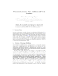
Figure 2.1.a shows a fragment of program code and Figure 2.1.b shows how this is
represented as a dataflow graph: circles represent instruction nodes, square represents a constant value and letters are variables.
Under the Von Neumann execution model, the program in Figure 2.1.a would execute sequentially in three steps. Whereas, under the dataflow execution model
the addition and the division are both immediately fireable, as all of their data is
initially present. The results are placed on the output arcs, that represent A and
B variables. Then the multiplication node becomes fireable and is executed. The
result is placed on the arc representing the variable C. In this scenario, a parallel
execution requires fewer steps than sequentially one.
Dataflow paradigm offers the potential to provide a speed improvement. Furthermore, if X and Y represent sets of data, the computation on the second series of
values can be started before those on the first series have been completed. This is
known as pipelined dataflow.
5
6
CHAPTER 2. BACKGROUND KNOWLEDGE
(a)
(b)
Figure 2.1: sequential vs dataflow program.
It’s interesting to underline, also, some disadvantages of using dataflow programming:
• the mindset of dataflow programming is unfamiliar to most professional programmers;
• if you need to convert an existent traditional program into data flow program then this could be very difficult especially for the fact that in data flow
paradigm there is not the concept of shared data structures.
The intent of this chapter is to provide a short introduction, by constructing a simple
example, to the most important features of the actor-based dataflow programming
paradigm using CAL and NL languages, for a more detailed description of the syntax
of these two languages see [2],[3].
2.1.1
CAL: the Caltrop Actor Language
In CAL an actor is a computational entity with input ports, output ports, state
and parameters. It communicates with other actors by sending and receiving tokens
along unidirectional connections. A model, or application, then consists of a network
of interconnected actors. When an actor is executed it is said to be fired [5]. During
a firing:
1. the actor may consume tokens from its input ports;
2.1. DATAFLOW PROGRAMMING
7
2. it may modify its internal state;
3. it may produce tokens at its output ports.
One way of thinking about an actor is as an operator on streams of data sequences
of tokens enter it on its input ports, and sequences of tokens leave it on its output
ports.
In order to underline the main features of the dataflow programming and CAL
language we build a simple example that consists of a network of actors which
computes the list of Fibonacci numbers. This network, shown in Figure 2.4, is
composed of three actors: one that adds two numbers (AddUntilOverflow) and
two delay blocks (SingleDelay). Since the adder block is more interesting than the
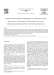
delay blocks we look inside of it. The first line of the Listing 2.1 declares an actor,
called AddUntilOverflow, followed by a list of parameters (empty in this case) and
the declaration of the input ports, called X and Y, and output ports, called Sum, all
of type int1 . The graphical representation of the actor AddUntilOverflow is shown
in Figure 2.2.
1
2
3
a c t o r AddUntilOverflow ( ) i n t X, i n t Y ==> i n t Sum :
...
end
Listing 2.1: simple actor.
Figure 2.2: graphical representation of the AddUntilOverflow actor.
The behavior of an actor is defined by its set of actions, in fact, a firing
consists of the execution of an action. An actor execution alternate the selection of
the next action to fire and the execution/firing of that action. An action declaration
is optionally preceded by an action tag in front of the keyword action. This label
is used to refer to the action, or to a set of actions, in fact this tag need not to
be unique. At this point the declaration is divided in two parts: the first one, in
1
CAL is optionally typed: the type declaration of a variable might be not present.
8
CHAPTER 2. BACKGROUND KNOWLEDGE
front of the =⇒ symbol, is a list of input patterns that defines how many tokens to
consume, from which incoming ports, and what to call those tokens in the rest of
the action. While the second one, in the right side of the =⇒ symbol, is a list of
output expression that specifies the number of and the values of the output tokens
that will be produced on each output port by each firing of the action. As shown
in Listing 2.2, the actor AddUntilOverflow has three actions called run, drain and
terminate. The first two take one token from each incoming port of the actor, but
only run produces a token on the outgoing port Sum, while the third action takes one
token from the Y input port, but, as drain action, doesn’t produce any token. The
idea behind the functionality of this actor is clearly suggested by its name and by
the design of the network: this actor adds two numbers until the arithmetic overflow
occurs (action run). When this happens the actor still has tokens at its input ports
(which are the products of previous addition). It consumes them without producing
other tokens (action drain), until it only have one token at one input port (action
terminate).
1
2
3
4
5
6
7
8
9
10
11
12
a c t o r AddUntilOverflow ( ) i n t X, i n t Y ==> i n t Sum :
run : a c t i o n X : [ x ] , Y : [ y ] ==> Sum : [ sum ]
...
var
i n t sum=x+y
end
d r a i n : a c t i o n X : [ x ] , Y : [ y ] ==>
end
t e r m i n a t e : a c t i o n Y : [ l a s t T o k e n ] ==>
end
...
end
Listing 2.2: simple actor with actions.
The only condition for an action to be fireable, so far, is that there are enough
tokens for it to consume as defined on its input patterns. There exist a nondeterministic behavior when two or more actions have sufficient input tokens to fire, and
the output will be different in agreement on which action it is chosen to fire. It’s
important to clarify that there aren’t rules to determine which action will be fired,
so, it’s possible to implement a nondeterministic actor, and it can be very powerful
when it is used responsibly!
CAL provides a set of additional criteria that need to be satisfied for an action
to be fired:
Guard contains a set of expressions that all need to be evaluate to true in order for
the action to be fireable. The guard conditions should be exhaustive, otherwise
that actor may reach a deadlock. While if they are disjoint we will obtain a
2.1. DATAFLOW PROGRAMMING
9
deterministic actor, otherwise a nondeterministic one;
Priority is a set of inequality that defines a partial order between actions, and this
order determines their firing precedence;
Schedule specifies a list of possible state transitions, each state transition consists
of the original state, a list of valid action and the target state. So a schedule
is a textual representation of a finite state machine.
1
2
3
4
5
6
7
8
9
10
11
12
13
14
15
16
17
18
19
a c t o r AddUntilOverflow ( ) i n t X, i n t Y ==> i n t Sum :
run : a c t i o n X : [ x ] , Y : [ y ] ==> Sum : [ sum ]
guard
sum >= 0
var
i n t sum = x+y
end
d r a i n : a c t i o n X : [ x ] , Y : [ y ] ==>
end
t e r m i n a t e : a c t i o n Y : [ l a s t T o k e n ] ==>
end
priority
run > d r a i n ;
end
s c h e d u l e fsm run :
run ( run ) −−> run ;
run ( d r a i n ) −−> d r a i n ;
d r a i n ( t e r m i n a t e ) −−> d r a i n ;
end
Listing 2.3: actor AddUntilOverflow.
In Listing 2.3 is shown a simple use of the three criteria presented above: in the run
action there is the guard sum ≥ 0. Note that the variable sum is what we want to
produce in the output, so, a guard conditions, in order to be evaluated, can peek
at the incoming tokens without actually consuming them. If it happens to be false
or the action is not fired for some other reason, and if the tokens aren’t consumed
by another action, then they remain where they are, and will be available for the
next firing. In relation to the meaning of behavior of this action, the aim of this
guard is to check when the arithmetic overflow event occurs. Indeed when this event
happens sum becomes < 0 and action run can’t fire.
Listing 2.4 illustrates the behavior of two actors which have non exhaustive and non
disjoint guard conditions:
1
2
3
4
a c t o r A( ) In ==> Out :
a c t i o n In : [ i n ] ==> Out : [ out ]
guard
in > 0
10
5
6
7
8
9
10
11
12
13
14
15
16
17
18
19
20
CHAPTER 2. BACKGROUND KNOWLEDGE
end
a c t i o n In : [ i n ] ==> Out : [ out ]
guard
in < 0
end
end
a c t o r B( ) In ==> Out :
a c t i o n In : [ i n ] ==> Out : [ out ]
guard
i n >= 0
end
a c t i o n In : [ i n ] ==> Out : [ out ]
guard
i n <= 0
end
end
Listing 2.4: actor A with non exhaustive guards and actor B with non disjoint guards.
The actor A will be in deadlock if it meets a zero token on its input port (guard
conditions not exhaustive), while the actor B will run in a nondeterministic way if it
meets a zero token on its input port (guard conditions not disjoint). In the case of
the AddUntilOverflow actor the exhaustivity clause is met and the disjoint clause
not, but this problem is resolved by the presence of a list of priority inequalities, in
this case by the only inequality run > drain. This means that the run action has
higher priority than the drain action, so if both are fireable the actor behavior will
be deterministic since it will fire the action with the highest priority.
In the end of the AddUntilOverflow actor, there’s a schedule declaration: a simple
way to understand it is to think of the finite state machine that it generates (Figure
2.3). The way to read this is that if the schedule is in run state (initial state) and
Figure 2.3: finite state machine for the AddUntilOverflow actor.
2.1. DATAFLOW PROGRAMMING
11
an action tagged with run occurs, then the schedule will stay in run state, while if
the schedule is in the same state and an action tagged with drain occurs, then the
schedule will changes its state to drain. Finally if the schedule is in drain state
and an action tagged with terminate occurs, then the schedule will remain in its
final state drain.
Now it’s possible to define the actor strategy to select the action to fire:
1. determine the set of suitable actions. Suitable actions are those that can
possibly be fired according to the schedule. If there is no schedule, then all
actions are suitable;
2. from those suitable actions, determine the subset of activated actions. An
action is activated if and only if it is suitable and the following conditions are
met:
(a) there are enough tokens available on the input ports to satisfy the input
patterns;
(b) all the guard expressions evaluate to true;
3. from the activated actions, determine the subset of fireable actions. An action
is fireable if and only if it is activated and there is no other activated action
with a higher priority.
Whereas there isn’t any policy for selecting the next action to execute among the
set of fireable actions any fireable action may be picked to be fired.
In Listing 2.5 there is the code of the other two components of the Fibonacci
network which we want to build, but it adds nothing to the discussion except for the
fact that here we can see the use of a parametric actor: SingleDelay actor has an
input parameter, called initialToken, whose meaning is to initialize the actor, so
in the case of Fibonacci network they will be initialized with the first two numbers
of the succession.
1
2
3
4
5
6
7
8
9
10
a c t o r S i n g l e D e l a y ( i n t i n i t i a l T o k e n ) i n t In ==> i n t Out :
i n i t : a c t i o n ==> Out : [ i n i t i a l T o k e n ]
end
run : a c t i o n In : [ x ] ==> Out : [ x ]
end
s c h e d u l e fsm i n i t :
i n i t ( i n i t ) −−> run ;
run ( run ) −−> run ;
end
end
Listing 2.5: actor SingleDelay.
12
CHAPTER 2. BACKGROUND KNOWLEDGE
2.1.2
NL: the Network Language
NL is a language for expressing algorithms that compute directed graph among
entities with ports, as expressed in [3]. A use of this language is the description
of dataflow system, that consist of several actors (the entities) connected by FIFO
channels, from an output port of an actor to an input port of another, along which
they pass tokens to each other. NL is designed in respect of three key features:
generality allows the description of arbitrary structures and algorithms computing
graph structures;
expressiveness: structures description is kept as simple as possible, but structures
representation may be complex;
target independence: NL is a general way to describe structures of the same kind,
such as dataflow networks or circuits.
To build a network of actors two main things needs to be done:
1. instantiate the number of actors required;
2. create the connections between them.
In addition, a network of actors can itself have input and output ports, which may
be connected to the ports of actors inside it.
The definition of a network, shown in Listing 2.6 is an example, starts similar
to that of an actor, with its name (Fibonacci), parameters (none in this case), as
well as input and output ports (none in this case). This is followed by a section,
introduced by the keyword entities, that instantiates the actors of the network
(actor instances are referred to by their instance names.): one AddUntilOverflow
actor and two SingleDelay actors (with parameter 1 and 0 respectively). In the
following section, introduced by the keyword structure, contains the definitions
of connections between actors. The representation of this declaration is shown in
Figure 2.4.
1
2
3
4
5
6
7
8
9
network F i b o n a c c i ( ) ==> :
entities
d1
= S i n g l e D e l a y ( i n i t i a l T o k e n =1);
d2
= S i n g l e D e l a y ( i n i t i a l T o k e n =0);
add = AddUntilOverflow ( ) ;
structure
add . Sum −−> d1 . In ;
d1 . Out −−> d2 . In ;
d1 . Out −−> add .X;
2.2. COMPILER DESIGN
d2 . Out −−>
10
11
13
add .Y;
end
Listing 2.6: simple Fibonacci network.
Figure 2.4: Fibonacci network.
It would of course be much more convenient to write a NL program for one
entire family of generalized network, for example the generalized Fibonacci number
generators network. In fact the network language provides a number of constructs
that allow the construction of parametric network structures. They are fully described in [3].
2.2
Compiler design
Modern compilers divide the compiling operation in two steps: front end and back
end. In the first step the compiler analyzes and translates the source code written in
a computer language (called source language) into an intermediate code. The second
step optimizes and translates the intermediate code into a executable binary code.
In some cases the compiler generates code in another computer language (called
target language) in order to create an executable program. The front end step is
divided in more phases:
• lexical analysis;
• syntactic analysis;
• semantic analysis;
• intermediate code generation.
Also the back end step is divided in more phases:
14
CHAPTER 2. BACKGROUND KNOWLEDGE
• data and control flow analysis;
• optimization;
• code generation.
The operation flow of a compiler is shown in Figure 2.5.
In this chapter techniques for designing a compiler front end are presented.
Figure 2.5: compiler design flow.
2.2. COMPILER DESIGN
2.2.1
15
Lexical analysis
In a compiler front end, the lexical analyzer, also called scanner, reads the source
code characters and it assembles them into expressive words, called lexemes. To
each of these lexemes coincide a token which consists of two components: a type
and a value (the lexeme). Therefore, a lexical analyzer takes a stream of characters
and produces a stream of tokens, that will be the input of the syntactic analyzer.
Figure 2.6 shows a possible execution of a scanner: the input is a code fragment
and the output is the produced stream of tokens. This example shows the most
Figure 2.6: tokens generation.
important tokens for a programming language like identifiers, separators, operators
and literals, as it’s shown in Table 2.1.
Type
Names
Lexemes
Identifier
ID
nEd nVer
Literal
INT
2
Operator
EQ SUB DIV
=-/
Separator LPAR RPAR SEMI
();
Table 2.1: typical token.
For any programming language it is possible to implement an ad hoc lexer, this
16
CHAPTER 2. BACKGROUND KNOWLEDGE
is done in a simple and readable way using a lexical analyzer generator. It specifies
lexical tokens using the formal language of regular expressions, implements lexers
using deterministic finite automata and use mathematics to connect the two.
Using regular expression it is possible to represent a regular language, that is set of
finite sequence of symbols (each sequence is called string) chosen from a non empty
set called alphabet. Table 2.2 shows the regular language L(R) generated by the
regular expression R, where is the empty string, | is the union operand, · is the
concatenation operand and ? is the Kleene closure.
Suppose, for example, that we want to recognize the language of identifiers and
R
L(R)
∅
a
{"a"}
R|S
L(R) ∪ L(S)
R·S
L(R) L(S)
∗
R
∅∪ L(R) ∪ L(R · R) ∪ . . .
(R)
L(R)
Table 2.2: language L described by the regular expression R.
integer numbers, so we can write this two regular expressions:
ID = [a − z][a − z0 − 9]?
NUM = [0 − 9][0 − 9]?
This means that an identifier, ID, is a letter (between “a” and “z”) followed by a
sequence (empty, finite or infinite) of letters and digits (between “0” and “9”). An
integer, NUM, is a digit followed by a sequence of digits2 .
It is possible to see that this rules are ambiguous, for example is max0 a single
identifier or an identifier followed by an integer number?
In order to answer to this question the common scanners use the following two
disambiguations rules:
longest match: the next token is the longest substring of the input that can match
a definition of a regular expression;
rule priority: the order of writing down the regular expression has significance, in
fact if two rules match the same input substring the next token is the regular
expression that is written first. So in this case max0 is an identifier by the
longest match rule.
2
note that in this way 0 . . . are valid integer numbers
2.2. COMPILER DESIGN
17
Regular expressions are common way to specify lexical tokens, but to understand how a scanner works we need a formalism that can be implemented by a
computer program. To do this it is possible to translate a regular expression to
a finite state automaton which recognize the tokens that we want. Below an automaton for recognizing identifiers is shown(Figure 2.7.a) and an automaton for
recognizing integer numbers (Figure 2.7.b) defined above like a regular expression.
In Figure 2.7.c we can see the merging of this two automata into a new automaton
that recognize both identifiers and numbers.
(a)
(b)
(c)
Figure 2.7: automata for the regular expressions recognition.
The implementation of an automaton is a mechanical task easily performed
by a computer, so it makes sense to have an automatic lexical-analyzer generator to
translate regular expressions into an automaton. JFlex is an example of this kind
of generators.
18
CHAPTER 2. BACKGROUND KNOWLEDGE
2.2.1.1
JFlex a scanner generator
JFlex is a lexical analyzer generator for Java written in Java, as expressed in [9]. It
permits a fast scanner generation and the design of fast generated scanners.
A JFlex specification file (.flex) generates a .java file that implements a scanner
class. It consists of three parts where is possible to declare user code, options and
declarations, and the lexical rules, divided by %%:
user code: consists of package declarations and import statements. It is copied
verbatim at the beginning of the scanner class.
%%
options: contains the directives and the java code to include in the generated lexer.
Each directive is situated at the beginning of the line and is preceded by the
% character. There are a lot of types of directives, for example this piece of
code
...
%public
%final
%class "classname"
%extends "classname"
...
tells JFlex to give the generated class the signature
public final class "classname" extends "classname".
These are some of the class options allowed by JFlex. Other important types
of options are the scanning method, the management of the end of file, the
CUP3 compatibility etc. . .
declarations: contains the specifications of lexical states and macros useful for the
last section of the .flex file. This section can define, thanks to the macros,
the regular expressions that will be recognized by the scanner. The way to
declare a macro is:
macro id = reg exp
A macro id is only a shortcut to refer to a regular expression in the lexical
rules section. For example with
...
Integer = [1 − 9][0 − 9]?
Identifier = [a − zA − Z][a − zA − Z0 − 9]?
3
a free parser generator.
2.2. COMPILER DESIGN
19
...
we tell JFlex that Integer is a non negative and non zero decimal number,
while Identifier is a letter in upper or lower case style followed by a sequence
of zero or more letters or digits. The operations allowed by JFlex are most
common operations between regular expressions like: union (|), concatenation,
Kleene closure (? ), iteration (+), option (?) etc. . .
%%
lexical rules: consist of a set of regular expression followed by an action (expressed
in Java code). During the running, the scanner consumes its input and determines the regular expressions that match the longest portion of the input
(longest match rule). If there are more than one, the generated scanner chooses
the expression that appears first in this section of the specification (priority
rule). After that it executes the associated action. If there is no matching regular expression, the scanner terminates the program with an error message.
For example the following declaration
...
"while"
{"code action"}
"for"
{"code action"}
{Integer}
{"code action"}
{Identifier} {"code action"}
...
tells the generated scanner that when the input matches with the string
"while" the related action will execute. This example shows, also, the use
of macros: input matches with an Integer if and only if it is generated by the
regular expression defined in the related macro.
JFlex generates exactly one file containing the scanner class in agreement to
the specification file. This class contains the Deterministic Finite Automaton tables,
an input buffer, the lexical states of the specification, a constructor, and the scanning
method with the user defined actions. The input buffer of the lexer is connected
with an input stream over the java.io.Reader object which is passed to the lexer
in the generated constructor. When it is called, it will consume input until either
an error occurs or the end of file is reached. In the later case the scanner executes
the EOF action, and returns the specified EOF value.
2.2.2
Syntactic analysis
The syntactic analysis phase is the process of analyzing a continuous stream of
tokens to determine its grammatical structure due to a given formal grammar. As
shown in Figure 2.8 the task of this step is executed by two important components:
20
CHAPTER 2. BACKGROUND KNOWLEDGE
Figure 2.8: syntactic analysis steps.
Parser: checks for the correct syntax and builds a data structure, called parse tree;
Abstract Syntax Tree builder: builds a simplified structure4 , called Abstract
Syntax Tree or AST, from the parse tree.
The leaves of the parse tree are the tokens found by the scanner, thus, what is
important in this kind of tree is how these leaves are combined to form the structure
of the tree and how the internal nodes are labeled.
In this context, the parser obtains a series of tokens from the scanner and verifies
that the series can be generated by the grammar of the source language. There
are two types of parsers which use a top-down (LL parser) or a bottom-up (LR
parser) approach. In either case, the string of tokens in the input of the parser is
scanned from left to right, one symbol at time. The syntax of programming language,
like expressions and statements, can be expressed by a context-free grammar. For
example, using a syntactic variable stmt to denote statements and the variable expr
to denote expression, the production
(2.1)
stmt → while ( expr ) { stmt }
indicates the structure of this type of control flow statement. Moreover, other productions must define what an expr is and what else a stmt can be.
In the formal definition, a context-free grammar consists of four components,
G = (N, T, P, S):
4
Simplified in the sense that it does not represent every detail that appears in the real syntax
(for example the parenthesis of an expression are not needed at this level).
2.2. COMPILER DESIGN
21
N: is the finite set of nonterminals symbols. A nonterminal symbol is a syntactic
variable that represents a phrase or a clause in a sentence (stmt and expr are
nonterminals);
T: is the finite set of terminals symbols. It specifies the alphabet of the language
definite by the grammar;
P: is the set of productions (or rules). A production specifies in which manner
the terminals and nonterminals symbols can combined to form strings. Each
production is composed of:
1. a nonterminal, called the head or left side of the production;
2. zero or more terminals and nonterminals, called body or right side of the
production. It describes how to is possible to construct the head of the
production;
S: is the start symbol that generates the grammar.
There are three operations to combine the terminal and nonterminal symbols: alternation (|), concatenation and repetition or Kleene closure (? ).
The construction of a parse tree can be made thanks to the derivation: beginning with the start symbol, each rewrite step replaces a nonterminal with the body
of one of its productions. There are two types of derivations: the first, called leftmost derivation, the first leftmost nonterminal in each production is replaced with
the body of one of its productions, in this case we talk about a LL parser, while, in
the rightmost derivation, the first rightmost nonterminal is chosen for the replacing,
so we talk about a LR parser.
A parse tree is a graphical representation of a derivation. Each internal node
of a parse tree represents the application of a production, in fact the internal nodes
are labeled with the nonterminal in the head of the production.
Suppose, for example, we have these productions
assign →
exp
→
|
|
|
|
ID EQ exp SEMI
exp DIV exp
exp SUB exp
LPAR exp RPAR
ID
INT
so, in Figure 2.9 it’s shown a representation of a parse tree obtained from these
(leftmost) derivations:
22
CHAPTER 2. BACKGROUND KNOWLEDGE
assign ⇒ ID(nEd) EQ exp SEMI ⇒
ID(nEd) EQ exp DIV exp SEMI ⇒
ID(nEd) EQ LPAR exp RPAR DIV exp SEMI ⇒
ID(nEd) EQ LPAR exp SUB exp RPAR DIV exp SEMI ⇒
ID(nEd) EQ LPAR ID(nVer) SUB exp RPAR DIV exp SEMI ⇒
ID(nEd) EQ LPAR ID(nVer) SUB INT(2) RPAR DIV exp SEMI ⇒
ID(nEd) EQ LPAR ID(nVer) SUB INT(2) RPAR DIV INT(2) SEMI
Figure 2.9: representation of a parse tree: circular nodes are the nonterminal symbols, while triangular nodes are terminal symbols.
In general, we say that a string belongs to a language L(G), generated by
grammar G, if it can be derived from the start symbol. Using mathematical formalism:
L(G) = {w ∈ T ? |S ⇒? w}
where ⇒? is the relation that represents the list of derivations that carry from a
nonterminal symbol to a string of terminal symbols.
2.2. COMPILER DESIGN
23
The parse trees aren’t optimally appropriate for compilation. They contain a
lot of redundant information, as parentheses, keywords, and so on. Hence, abstract
syntax trees are generally used. Abstract syntax tree omits the irrelevant details,
but keeps the essence of the structure of the text. It is a tree structure where each
node corresponds to one or more nodes in the parse tree. For example, the parse tree
shown in Figure 2.9 may be replaced by the abstract syntax tree shown in Figure
2.10:
Figure 2.10: abstract syntax tree.
Exactly how the abstract syntax tree is represented and built depends on the
parser generator used.
2.2.2.1
Beaver: a parser generator
Beaver is a Look-Ahead LR parser generator [10]. LR parsers give the fastest parsing speed, but they are considered impracticable because the automaton that they
implement require huge number of states. LALR parsers offer the same high performance as LR parsers, but are much smaller in size, since they reduce the number
of states in an LR parser by merging similar states. For this reason, LALR parsers
are most often generated by compiler generators.
Beaver takes a context-free grammar and converts it into a Java class that
implements a parser for the language described by the grammar. This parser will
perform a syntactic analysis and assemble input tokens (supplied by a scanner) into
structures as described by the production rules of the language specification.
Like JFlex, Beaver also allows the programmer to declare directives that are
used to customize the generated parser or declare how some symbols will be used in
the grammar. This part must be specified before production rules, in the followings
24
CHAPTER 2. BACKGROUND KNOWLEDGE
are some examples of these directives:
%package "package.name"; declares the parser package name.
%import "package or Type"[,"package or Type" ...]; declares which Java packages and types should be imported.
%class "ClassName"; declares the name of the Java class for the generated parser.
The parser main aim is to match symbols to their definition. Therefore the
bulk of a specification usually is represented by production rules that combined
represent the grammar of a language that the generated parser will recognize. Each
rule declares a nonterminal symbol (on the left-hand side) and a sequence of other
symbols (on the right-hand side of =) that will produce the nonterminal:
symbol = symbol a symbol b ...{:
action routine code :};
Beaver allows the altering of the meaning of right-hand side symbols by marking
them with the following special characters:
? the symbol is optional;
+ the symbol represents a nonempty list of symbols;
∗ the symbol represents a possibly empty list of symbols.
The “action routines” will be called when all the symbols on the right-hand
side are matched and are ready to be reduced to a single nonterminal from the
left-hand side of the rule. Action routine creates and returns the symbol node that
will become accessible as a symbol of some other production’s right-hand side. To
exemplify the AST building process consider the following grammar:
Exp =
|
|
;
Exp.a MUL Exp.b {: return new MulExp(a,b); :}
Exp.a ADD Exp.b {: return new AddExp(a,b); :}
INT.i
{: return new IntExp(i); :}
Figure 2.11 shows the AST for the expression 5 + 7 ∗ 60. When return new
AddExp(a,b); is executed, it means that the expressions a and b were available
as symbol nodes, a new AddExp node is created (with two child: a and b) and its
reference is now open for the right-hand side production that contains it.
Beaver defines a simple interface that it expect scanners will follow in order
to feed it with tokens. Scanner returns the next token it finds in the input when
2.2. COMPILER DESIGN
25
Figure 2.11: abstract syntax tree for the expression 5 + 7 ∗ 60.
parser calls nextToken method.
Moreover the Beaver’s parsing engine uses simple token stream repairs and a phraselevel error recovery in order to recover from a syntax error. Parse grammars are
specified in .parser files.
2.2.2.2
JastAdd: a compiler compiler system
JastAdd is an open source Java-based compiler compiler system [12]. The main
design idea behind JastAdd is to make a specification formalism, called Rewritable
Circular Reference Attributed Grammars(ReCRAGs) easily accessible to Java programmers. For this reason, JastAdd uses a syntax very close to Java. It is designed
to work with any Java-based parser generator that supports user-defined semantic
action, as JavaCC, CUP, and Beaver. AST is specified in .ast file and represents
a set of Java class hierarchy, thus it allows behavior to be defined in classes and
specialized in subclasses. In a JastAdd class hierarchy there are three predefined
java classes as shown in Table 2.3. Furthermore, in order to create a class hierarchy,
Class
ASTNode
List
Opt
Use
topmost node in the hierarchy, each other class extends it
implement lists
implement optionals
Sintax
className∗
[className]
Table 2.3: JastAdd predefined Java classes.
JastAdd provides some basic syntax constructs, as:
abstract A; ⇒ produces an abstract class A, that corresponds to a nonterminal;
B : A ::= A [B] C∗ <D>; ⇒ produces a class B, that is an extension of A, thus
B is a production of A. Moreover, B has four children of types A, an optional
child of type B, a list of children of type C and a token child of type D.
26
CHAPTER 2. BACKGROUND KNOWLEDGE
JastAdd is used for doing computations on an AST. In a traditional compiler,
you create external data structures like symbol tables and alternative program representations like flow graphs. In JastAdd, you represent all those things directly in
the AST using attributes. These and other JastAdd features is presented in Section
2.2.3.1.
2.2.3
Semantic analysis
In the semantic analysis phase the compiler adds semantic information to the AST.
At this point the analysis can be divided in the following two main analysis steps:
Name Analysis: in a programming language, each object (as variables and functions) has a declaration, that is a name used to refer to the object. Moreover,
each name also have a number of uses, inside the source code, each of which is
a reference to the named object in order to compute the goal task. Associating
use and declaration is called name binding and it is shown in Figure 2.12.
If a declaration of a name is not visible in the entire program it has a restricted
scope then that declaration is called local. On the contrary, if it is is visible in
the entire program code than the declaration is called global.
To do name binding symbol tables are used. They are useful to bind the identifiers uses to their declarations. In some languages (as CAL) a variable and a
Figure 2.12: name binding example.
function in the same scope may have the same name, as the context of use will
make it clear whether a variable or a function is used. In order to discriminate
which are variables and which are functions we say that they have separate
name spaces, which means that their name sets are disjoint. Usually each
2.2. COMPILER DESIGN
27
name space corresponds a symbol table, but nothing prevents us from sharing name spaces using just one symbol table, but this case needs additional
information in order to avoid confusion between different name spaces.
Type Analysis: in this step a compiler must compute the type for each expression
in the source code in order to check if it has the correct type in the context
where it is located. For example a possible way to do this task may be the
following:
Exp1 + Exp2
Exp1 = Exp2
...
t1 =checkExp(Exp1 )
t2 =checkExp(Exp2 )
⇒ if t1 =int and t2 =int
then int
else error()
t1 =checkExp(Exp1 )
t2 =checkExp(Exp2 )
⇒ if t1 =t2
then bool
else error()
⇒ ...
As seen in the example above, at this point it is necessary to have, at least,
a representation of predefined types available in the language. Thus, we can
create a constant object for each type as:
1
2
3
4
5
i n t e r f a c e PredType {
p u b l i c s t a t i c f i n a l PredType intType=. . . ;
p u b l i c s t a t i c f i n a l PredType boolType=. . . ;
...
}
This interface is useful, thanks to the object-oriented nested class, to create
the type conversion rules. For example, in Figure 2.13 is shown the Java conversion rule, that is a widening conversions, which are intended to preserve
information. The widening rules are given by a hierarchy of class: any type
lower in the hierarchy can be widened to a higher type. Thus, a char can be
widened to an int or to a float, but a char cannot be widened to a short.
Essentially, the compiler, in this step, must determine that these type expressions conform to a collection of logical rules that is called the type system for
the source language.
During the semantic analysis the analyzer may discover some types of errors:
• names uses without declaration;
28
CHAPTER 2. BACKGROUND KNOWLEDGE
Figure 2.13: Java widening conversion rule.
• multiple declaration of the same name in the same block;
• type expression errors.
2.2.3.1
JastAdd aspects
Usually, semantic analysis is performed by adding aspects to the AST. JastAdd
aspects support declarations that are written in an aspect file, but that actually
belongs to an AST class, these declarations are called intertype. The JastAdd
system reads the aspect files and weaves the intertype declarations into the appropriate AST classes, as shown in Figure 2.14. The aspect files contain ordinary Java
methods and fields, and attribute grammar constructs like attributes, equations, and
rewrites. An aspect file can have the suffix .jadd or .jrag. There is not difference
between this two types of files but it is recommended for the following use:
• in a .jrag file we add attributes, equations, and rewrites to the AST classes,
thus for declarative aspects;
• in a .jadd file we add ordinary fields and methods to the AST classes, thus
for imperative aspects.
As in attribute grammars, attributes are declared in AST classes, and their values
are defined by equations. An attribute is either synthesized, if it is used for propagating information upwards in the AST, or inherited, otherwise.
A synthesized attribute is analogous to an ordinary virtual method: the attribute
declaration corresponds to the method declaration, and the equations to the method
implementations.
Inherited attributes are used for passing information downwards in an AST, giving
2.2. COMPILER DESIGN
29
Figure 2.14: Architecture of the JastAdd system.
child nodes information about their context.
A typical example is that information about visible declarations, usually called the
environment is passed down to each statement, which in turn passes down this information to the variables inside it. A variable can use this environment information
to find its declaration and type.
2.2.4
Intermediate code generation
The final goal of a compiler is to allow programs written in a high-level language to
run on a computer. Thus, compilers perform the translation from a high-level to a
machine code language.
Suppose, for example, we want compilers for N source languages and we have M
target machine, then we should implement N · M compilers (Figure 2.15.a). Many
compilers use a medium-level language, called intermediate code or intermediate
representation (IR), between the high-level language and the very low-level machine
code. In this solution we have to implement only N + M compilers (Figure 2.15.b),
in fact N front ends of the compiler do lexical analysis, parsing, semantic analysis,
and translation to intermediate representation, while M back ends do optimization
of the intermediate representation and translation to machine language.
However, this solution produces an increasing of the information overhead that in
some cases reduces the translation speed.
30
CHAPTER 2. BACKGROUND KNOWLEDGE
(a) without IR
(b) with IR
Figure 2.15: compilers for four source languages and two target machine.
An intermediate language should, ideally, have the following properties:
• it should be easy to translate from a high-level language to the intermediate
language;
• it should be easy to translate from the intermediate language to machine code.
• the intermediate format should be suitable for optimizations.
The first two of these properties can be somewhat hard to reconcile, so a language
that is intended as target for translation from a high-level language should be fairly
close to this.
2.2.4.1
XLIM: a XML Language-Independent Model
XLIM is a XML format for representing a language independent model of imperative
programs. It is essentially equivalent to a program in static single assignment (SSA)
form, in which each variable is assigned to in only one place of the source [6].
The root level of a XLIM document is the design element (there must be only one
per document) and it consists of three main types of elements:
1. a list of port elements that define how data travel to and from the functionality
block represented;
2. a list of program states (called state variables) that represent persistent
storage for the design and they are accessible from any portion of the design;
3. a collection of modules and operations. Modules can contain operations
and/or other modules in order to create a hierarchy of arbitrary depth. They
2.2. COMPILER DESIGN
31
are used to define control flow within the design. Whereas, operations are the
atomic unit of functionality, their execution depend on availability of data.
To show a simple example of intermediate code generated for the actor in the
Listing 2.1 we quote the following little piece of code, that declares a XLIM design
called AddUntilOverflow with three actor ports:
1
2
3
4
5
6
<d e s i g n name=AddUntilOverflow>
<a c t o r −p o r t d i r=" i n " name="X" s i z e="32" typeName=" i n t "/>
<a c t o r −p o r t d i r=" i n " name="Y" s i z e="32" typeName=" i n t "/>
<a c t o r −p o r t d i r="out" name="Sum" s i z e="32" typeName=" i n t "/>
...
</d e s i g n >
Listing 2.7: intermediate code generated for AddUntilOverflow.
When we declare an actor-port we define an element of the interface to the design.
An actor-port is a conceptual port, it is implemented as simple I/O, or a complex
port that requires a protocol. Accesses to the port are achieved by pinRead and
pinWrite operations. For a more detailed specification of these and other XLIM
features [6] is a recommended reading.
32
CHAPTER 2. BACKGROUND KNOWLEDGE
Chapter 3
Developed work
3.1
Scanning
As seen in section 2.2.1.1 a scanner is defined by a list of regular expressions that will
recognize significative strings of characters. CAL and NL, as most of the common
languages, have the following kinds of lexical tokens: keywords, identifiers, operators, delimiters, comments and numeric literals. For example, the following regular
expression defines the identifier token class using JFlex syntax:
Alpha
= [$A-Z a-z]
DecimalDigit = [0-9]
Identifier
= {Alpha}({Alpha}|{DecimalDigit})∗
When the scanner matches a regular expression it returns the related symbol
defined by the parser in the context-free grammar. For example, when an identifier
is matched the scanner executes:
return sym(Terminals.IDENTIFIER);
which creates and returns an object Symbol that represents the token.
Terminals.IDENTIFIER is declared in the concrete grammar.
3.2
Parsing
In order to build the parse trees for CAL and NL you must specify their context-free
grammars. Thus, this step involves a study of the syntax of the two languages. CAL
33
34
CHAPTER 3. DEVELOPED WORK
syntax is specified in the Appendix A of [2] by a list of productions divided into five
class rules:
1. Actor: specifies the rules to declare an actor, imports, variables and functions;
2. Expressions: specifies how to build expressions and special CAL constructs;
3. Statements: describes the syntax for the use of CAL statement constructs;
4. Actions: describes the rules to declare actions;
5. Action control: specifies the CAL constructs for the action control flow.
NL syntax is expressed in [3] and it is divided into three class rules:
1. Network: specifies the rules to declare a network;
2. Entities: describes how to define the entities that make up the network nodes;
3. Building structure: specifies the rule to define the structure of the network.
Moreover, NL uses some elements of CAL, for example Expressions and Statements.
I have developed two Beaver context-free grammars by the translation of these
rules in agreement to the Beaver syntax. For example this CAL production
PortDecl → [multi] [Type] ID
specifies that a port is an optionally terminal symbol multi followed by an optionally nonterminal symbol Type followed by an identifier declaration, represented
by the nonterminal symbol ID. It is translated into this Beaver production:
PortDecl port decl
=
multi? type? id decl
{: return new PortDecl(multi,type,id decl); :};
that allows the parser to build a new PortDecl node when the input stream of
tokens match to the right-hand side of the production.
3.3
Abstract Syntax Tree
The .ast files that contain the abstract grammar descriptions are very similar to
a list of productions, as in the case of a context-free grammars, specified in the
3.3. ABSTRACT SYNTAX TREE
35
.parser files. But the abstract grammar has the power to “prune” the parse tree1
by all those nodes that are unnecessary, and to specialize other nodes.
A classical example of these aspects are the specialization of expression nodes with
the consequent omission of operation terminal symbols from the tree. The following
Beaver productions
Expression
expression=
binary exp;
Expression binary exp=
and exp
|
expression.e1 OR and exp.e2 {:return new OrExp(e1,e2);:};
Expression and exp=
equal exp
|
and exp.e1 AND equal exp.e2 {:return new AndExp(e1,e2);:};
...
use nonterminal symbols that are defined in the following abstract grammar:
abstract Expression;
abstract ExpressionBinary : Expression ::= LOp:Expression ROp:Expression;
abstract BooleanExp : ExpressionBinary;
AndExp : BooleanExp;
OrExp : BooleanExp;
...
JastAdd creates three abstract classes and two concrete classes with this relation
between them:
Expression
↑
ExpressionBinary
↑
BooleanExp
%AndExp OrExp
where the arrow represent the function “is a”.
1
the parse tree is not created: when the parser parses a stream of tokens it directly build the
AST. The pruning is referred only to the fact that unnecessary tokens are not used in the AST,
so they are pruned.
36
CHAPTER 3. DEVELOPED WORK
An abstract grammar makes a clean interface between the parser and the later
phases of a front end. It keeps the essence of the structure of the text but omits the
irrelevant details. In an abstract syntax tree, interior nodes represent programming
constructs, while in a parse tree, interior nodes represent nonterminals. A designer
of a front end has much freedom in the choice of abstract grammar. As expressed
in [8], some use an abstract syntax that retains all of the structure of the concrete
syntax tree plus additional positioning information used for error reporting. Others
prefer abstract syntax that contains only the information necessary for compilation,
skipping parentheses and other irrelevant structure. Based on the semantic meaning
of each CAL construct, my abstract grammar separators, operators and almost
all keywords are dropped. To exemplify this choice, consider the port declaration
construct which syntax is:
PortDecl → [multi] [Type] ID
If, in the source code, the keyword multi is not specified then it means that that port
is single. A single port represents exactly one sequence of input or output tokens.
Otherwise it specifies a multi port, that represents any number of those sequences.
Thus, this is an example of a keyword that must not be omitted in the abstract
grammar since it has an important semantic meaning. The previous production is
equivalently translated in the following one contained in the abstract grammar, in
agreement with the JastAdd syntax:
abstract PortDecl ::= [Type] IdDecl;
PortDeclSingle
:
PortDecl;
PortDeclMulti
:
PortDecl;
or alternatively:
PortDecl ::= [<MULTI:String>] [Type] IdDecl;
In the first case, when the parser matches the right hand side of the production
with the multi keyword it creates and returns a PortDeclMulti node, otherwise
a PortDeclSingle node. In this case JastAdd generates one abstract class for
PortDecl and two subclasses: one for PortDeclSingle and one for PortDeclMulti
nonterminal symbol. Whereas, in the second case it generates a java class for
PortDecl nonterminal symbol that has, as child, the token which represents the
multi keyword. First solution is probably better than second one because it reduces the number of nodes in the tree, but, as first implementation, I chose the
second way in order to keep the class hierarchy as smaller as possible. Using this
procedure, based on the semantic meaning of each symbol of the concrete grammar,
I wrote the complete abstract grammar for CAL and NL language.
3.4. SEMANTIC ANALYSIS
3.4
37
Semantic analysis
This section describes how I implemented name analysis and type checking for the
CAL language main constructs.
First I want to clarify that, in my implementation, these two phases are not realized
by two aspects which traverse the abstract syntax tree in two different moments,
but checking is launched by name analysis at the when needed, this will become
clear in subsection 3.4.5.
Name analysis is realized by CalNameBinding.jrag aspect and it uses other
aspects to do its task. In order to bind identifier uses to its declaration this aspect
adds this attribute:
public IdDecl IdUse.decl;
JastAdd will add the attribute decl, of type IdDecl, in the IdUse class. This new
attribute will represent the reference to the identifier declaration (as shown in Figure
2.12).
Name analysis and type checking start their execution when nameBinding()
method in Actor main class is called, from then running proceeds by the execution
of eight steps described in the next subsections.
3.4.1
Namespaces creation
Using an auxiliary structure, called symbol table, I defined five different namespaces
for input ports, output ports, functions, variables and actions names. The symbol
tables are implemented as a stack of hash maps, as explained in [7], where a new
hash map is pushed on the stack when the analyzer enters a block and is popped
when it leaves the block. A symbol table supports seven main operations:
• void add(String symbol, Object meaning): adds the symbol and its associated
meaning to the top symbol table;
• boolean alreadyDeclared(String symbol): returns true if the symbol is already
in the symbol table;
• int blockLevel(): returns the numbers of hash maps in the stack;
• void enterBlock(): pushs a new hash map to the stack;
• void exitBlock(): pops the top hash map from the stack;
38
CHAPTER 3. DEVELOPED WORK
• Object lookup(String symbol): returns the meaning of symbol if it is in the
table null otherwise;
• Set<String> keySet(): returns all the symbols in the table.
In particularly, in this case, the meaning is represented by IdDecl node of the AST.
Thus to perform the name analysis an analyzer must, first, traverse the tree to look
for each identifier declaration and put in the symbol table. Secondly it makes the
binding between uses and declaration of an identifier. At the end the symbol tables
are empty.
3.4.2
Port name setting
This phases, realized by CalPortName, is necessary to allow the analyzer to bind
the ports in actions to the ports in the actor signature. The following is a piece of
AST declaration present in .ast file:
ActorHead
PortDecl
Action
Input
Output
Import∗ Identifier TypePar∗ DeclPar∗ Input:PortDecl∗
Output:PortDecl∗ [Time];
::= [Multi] [Type] IdDecl;
::= [QualIdDecl] Input∗ Output∗ [Guards] [Delay]
DeclVariable∗ Statement∗ ;
::= [IdUse] IdDecl∗ [Repeat] [Channel];
::= [IdUse] Expression∗ [Repeat] [Channel];
::=
in the Input and Output productions IdUse represents the name of an actor ports.
Thus, the aim of this step is to create an IdUse child, if not yet present, in Input
and Output nodes in order to be able to bind that use to the related declaration
contained in PortDecl. The binding is either by name, if IdUse child is present,
or by position, otherwise. For example, the Run action in the Cell actor declared
in the Listing 3.1 has a list of tokens, but it is not specified from which ports they
come from. After this step the first token (nw) will be associated to the first port
(NW), and so on. . .
3.4.3
Declarations adding
This is really the first phase of name analysis. Here, the analyzer scan the entire
abstract syntax tree in order to find global name declarations and adds them in
the correct symbol table. In a CAL program the global names are: state variables,
functions, procedures, ports name and action tags. Consider Listing 3.1:
3.4. SEMANTIC ANALYSIS
1
2
3
4
5
6
7
8
9
10
11
12
13
14
15
16
17
18
19
20
21
22
23
24
25
26
27
28
39
a c t o r C e l l ( i n i t ) NW, N, NE, W, E , SW, S , SE ==> Out :
s t a t e := n u l l ;
I n i t : a c t i o n ==> Out : [ s t a t e ]
do
s t a t e := i n i t ;
end
Run : a c t i o n [ nw ] , [ n ] , [ ne ] , [ w ] , [ e ] , [ sw ] , [ s ] , [ s e ] ==> [ s t a t e ]
var
count = sum ( [ nw , n , ne , w, e , sw , s , s e ] )
do
i f s t a t e = 0 then
i f count = 3 then
s t a t e := 1 ;
end
else
i f count < 2 o r count > 3 then
s t a t e := 0 ;
end
end
end
s c h e d u l e fsm s 0 :
s 0 ( I n i t ) −−> s 1 ;
s 1 (Run) −−> s 1 ;
end
f u n c t i o n sum (L) :
accumulate ( lambda ( x , y ) : x + y end , 0 , L)
end
end
Listing 3.1: adding global declarations.
The global declarations and the related namespaces are shown in Table 3.1. Note
that the name declaration init will be inserted in two different symbol tables, since
it is not possible (at this point) to discriminate if it is a variable declaration or a
function declaration. Local declarations will be added to the related symbol table
during the name binding phase.
3.4.4
FSM transformation
When syntactic analyzer parses a CAL schedule construct it builds a tree unsuitable
for the name analysis. For example look at the schedule declaration in the Listing
3.2. The abstract syntax tree built by the parser is very similar to that one shown in
Figure 3.1.a, where it is possible to see that a transition is an initial state followed
by one or more action tags followed by a target state. we can raise the following
two question: which of those names are declarations and which of those names are
40
CHAPTER 3. DEVELOPED WORK
Decl Line
Table
init
1
variable, function
NW
1
input
N
1
input
NE
1
input
W
1
input
E
1
input
SW
1
input
S
1
input
SE
1
input
Out
1
output
state
2
variable
Init
3
action
Run
7
action
sum
25
function
Table 3.1: name declarations and their related symbol table.
uses? And, what action or actions the name do refers?
1
2
3
4
5
6
7
8
9
10
11
12
a c t o r A ( ) IN ==> OUT :
s t a r t : a c t i o n ==> . . .
do . down : a c t i o n ==> . . .
do . up : a c t i o n ==> . . .
done : a c t i o n ==> . . .
...
s c h e d u l e fsm i n i t :
i n i t ( s t a r t ) −−> run ;
run ( do ) −−> run ;
run ( done ) −−> i n i t ;
end
end
Listing 3.2: schedule declaration example.
As seen, using this schedule declaration syntax an action tag may refers to a set
of actions. Thus, the previous schedule declaration is equivalent to that shown in
Listing 3.3.
1
2
3
4
5
s c h e d u l e fsm i n i t :
i n i t ( s t a r t ) −−> run ;
run ( do . down , do . up ) −−> run ;
run ( done ) −−> i n i t ;
end
3.4. SEMANTIC ANALYSIS
41
Listing 3.3: equivalent schedule declaration.
For a name analyzer is easy to directly bind the action tags used to their declarations
in the action signatures with the second schedule declaration, but it’s impossible with
the first one. Moreover states are implicitly declared states and also they are used
to define a finite state machine. To avoid these problems the code in CalFSMTransf
aspect operates a rewriting of this subtree.
In this new representation a finite state machine is a list of state transitions, each
transition declares its initial state, as a left child, and a list of transition bodies. A
transition body is a list of action tags followed by a name of a target state (now
a name analyzer is able to bind state uses to their declarations). Each action tag
contain a vector of references to the related action tag declaration in the action signature. Moreover, the name declaration as left child of the first transition represents
the initial state of the finite state machine.
References vector filling is an assignment of the name binder. A reference is added
into the vector whenever an action tag use matches to a declaration contained in
the action names symbol table. If an action tag use is a prefix of an action tag
declaration then there is a matching.
In Figure 3.1.b is shown the result of this transformation. This new subtree
will replace the old one.
42
CHAPTER 3. DEVELOPED WORK
(a)
(b)
Figure 3.1: Finite State Machine subtree.
3.4.5
Name binding
This is the core of name analysis and the code is contained in CalNameBinding
aspect. By recursive traversal among the AST the analyzer should, firstly, look
for any local declarations, that adds to the correct symbol table, secondly, look for
any IdUse node and, thirdly, call the routine dedicated to the type checking when
3.4. SEMANTIC ANALYSIS
43
necessary. When a IdUse node is found this piece of code is executed:
decl=(IdDecl)table.lookup(getIdentifier().getID());
thus, the analyzer looks for the current identifier use in the table that represent the
namespace of the declared identifiers. If it find the related declaration set the IdUse
binding attribute to the value of the IdDecl node that contains the name declaration,
otherwise it reports a “MISSING DECLARATION” error message. The analyzer
behavior described above is not the same for each node in the AST, in fact we can
distinguish four types of nodes:
• class A: all nodes that contain local variable or function declarations and
that require a name binding analysis for each child. For example, actions are
instances of this class;
• class B: all nodes of class A that needs type checking. An example of an
element of this class is the while statement construct, i.e. the local variable
declarations must be added and the condition must be boolean;
• class C: all nodes that require name binding analysis for each child and type
checking, but they have not local declarations. For example, if statement
constructs represent an element to this class;
• class D: schedule and priority declarations.
Summarizing:
Class Add Declarations Name binding
A
yes
yes
B
yes
yes
C
no
yes
D
no
yes
Type checking
no
yes
yes
no
Whenever the analyzer meet a class A or B node it pushes a new dictionary
in the symbol table, this means that those declarations have a limited scope. So
they are visible only for the uses that the analyzer meets in the next name binding
analysis. After that the analyzer pops the top dictionary from the symbol table and
its declarations are no longer available to be binded.
44
3.4.6
CHAPTER 3. DEVELOPED WORK
Type assignment
This step is integrated with name binding and declarations adding steps. When the
analyzer finds an IdDecl node and pushes it in the correct symbol table, it also, tries
to assign it a type. The type hierarchy is defined in an auxiliary class structure.
It is specified in ObjectType.java class contained in semanticlib directory and
its graphical representation is shown in Figure 3.2. An arrow, that connects two
Figure 3.2: hierarchy types representation.
different type classes, represents the function “is a”. Thus, for example a Char is a
String that is an Object.
To perform the type assignment task I added an attribute to the IdDecl class in
this way:
public ObjectType IdDecl.type;
The attribute will contain the type of the current declaration. To assign a type the
analyzer simply tries to find a string that matches a type declaration, for example
int i is a Int object. CAL is a optional typed language, so a type declaration may
be omitted, in this case, that declaration has type unknown.
3.4.7
Type checking
When the analyzer meets a node that needs a type checking, it executes the code
that is specified in the CalTypeChecking aspect.
During the name binding step, when the analyzer requires a type checking for a
3.4. SEMANTIC ANALYSIS
45
node then this means that it has met a particular CAL construct that requires a
particular type, as a guard or a repeat construct, or the current node has a class
IdUse as child.
The following table shows the operations that the analyzer executes when it met a
Repeat node:
Node
Repeat
Operation
t=getExpression().getExpressionType();
if(!t.isIntType()) then error();
Note that operations between types, as isSubtype() or isBoolType(), are
implemented in the ObjectType.java class.
An objects t1 of type ObjectType may check if it is a same type of another object
t2 , of type ObjectType, calling isSameType(t2 ) method, and, also, t1 may check if
it is a subtype of t2 by calling the isSubtype(t2 ) method. Moreover, t1 may check
if it is of a certain type calling the is<type name>Type() method or if it is of a
certain subtype calling the is<type name>Subtype() method.
Errors launched by the analyzer, at this computation step, are represented by
strings printed in a XML form. For example this error message
<Check Type Repeat>
<ERROR type= CAL. Object . Unknown l i n e= ( 5 0 , 2 0 ; 5 0 , 2 7 ) / >
</Check Type Repeat>
tells that in the repeat clause at line (50,20;50,27) the analyzer found a unknown object instead of an integer. Line informations are printed by the lineCol() method,
implemented in the SourceLine aspect, which is available for each class in the hierarchy defined by AST.
3.4.8
Expression type computation
This is the last step of the name and type checking analysis and it performs the task
of returning a type of an expression.
CAL provides four main expression constructs that in the AST are represented by
particular nodes:
• binary expressions consist of a left expression and a right expression child.
The analyzer must evaluate their type and checks if the operation has the
correct operand. At the end it returns the expression type.To exemplify look
at this table:
46
CHAPTER 3. DEVELOPED WORK
Binary Exp
BooleanExp
Op1
Op2
Return
bool
bool
bool
bool
unknown unknown
unknown
bool
unknown
unknown unknown unknown
It shows the accepted operand types for a boolean operation (as and), and the
returned type;
• unary expressions consist of a only one expression child. Thus, analyzer
behavior is fairly near to the previous one;
• expression literals represent the constant value of an expression. Thus their
type is implicitly defined in what they are. For example an integer literal
belongs trivially to the Int class;
• other constructs are provided by the CAL language, as if-expression, letexpression, lambda-expression, etc. . .
They should be treated case by case but the basic idea remains the same:
analyze expressions child, check if they have the correct type and return the
expression type. The following table exemplify this concept for if-expressions:
Expression
IfExp
3.5
Operations
1) checks if ’if’ expression is boolean
2) checks if ’then’ expression is a subtype
of the ’else’ expression or vice versa
3) launch an error or return the higher type
class found
Intermediate code generation
In this section, I illustrate a scheme for generating intermediate code. The source
code used to generate an intermediate representation is contained in the CalToXLIM
aspect.
This intermediate code generation step is done after the previous analysis.
This process starts when the writeXLIM(String filename) function, in the Actor
class, is called. The process traverse the AST in order to translate the attributed
AST into a XLIM intermediate representation. This task is summarized by the
following list of step:
1. open a new design block;
3.6. TESTING
47
2. add actor-port declarations blocks;
3. add action declarations blocks:
(a) add a pinRead operation block for each incoming port;
(b) add operation blocks to compute the outputs tokens;
(c) add a pinWrite operation block for each outgoing port.
4. add finite state machine declaration blocks in order to specifies action firing
rules:
(a) add a stateVar block that represents the current state of the state machine;
(b) add operation blocks to represent the finite machine states;
(c) add an infinite loop module that represents the finite machine running.
In the body of this loop for each action:
i. add a pinAvailable operation block for each incoming port
ii. if the action is guarded add a pinPeek operation block for each incoming port, then add the operation blocks necessary to evaluate all
the guards;
iii. add an and operation between the exits of pinAvailable and guard
blocks;
iv. add a pinAvailable operation block for each outgoing port;
(d) add a series of module and operation that implement the schedule defined
by the finite state machine.
3.6
Testing
In order to test my work I created, using JUnit, a test framework class, named
TestAll.java contained in testframework directory. It looks for all the classes in
the project that extend the TestCase class and it run them. Thus, it is easy to
add new test classes. At the moment the only available test class is contained in
test directory and it is named ParserTest.java. The functionality of this class
is to parse and execute name binding (and type checking) for all .cal files in the
data directory, while for all .nl files in that directory this class execute the parsing.
At the end of the execution two log files are produced in the output directory:
out test.log and err test.log. Both are written in a XML mode, and both
show the computational results during all the analysis phases. The first one shows
the successful executed operations and the second one shows the errors launched by
the analyzer. The following is an example of successful operation:
48
CHAPTER 3. DEVELOPED WORK
<Bind idUse= a i d D e c l= a l i n e s= ( 5 2 , 1 6 ; 5 2 , 1 6 ) , ( 5 0 , 1 7 ; 5 0 , 1 7 ) / >
which inform us that the use of name a in line (52,16; 52,16) is successfully binded
to the name declaration in line (50,17; 50,17). Whereas an example of error is:
<Check Type Repeat>
<ERROR type= CAL. Object . Unknown l i n e= ( 5 0 , 2 0 ; 5 0 , 2 7 ) / >
</Check Type Repeat>
which informs us that during the type checking the type of the expression in a repeat
clause is evaluated unknown instead of int. Another type of error is shown in this
way:
<MISSING DECLARATION idUse= complex l i n e= ( 6 1 , 9 ; 6 1 , 1 5 ) / >
which informs us that the use of the name complex does not have declaration in the
.cal file.
In the test folder there is another class file, called Cal2XLIM.java. This is
the main class of the project. It receives a CAL project as input and parses all
files and generates, from .cal files, a folder, called compiled, that contains all the
intermediate representations (.xlim files).
Chapter 4
Final remarks
4.1
Conclusion
At the beginning of this thesis I did not have much knowledge about compiler design,
CAL, or Network language. Therefore, after an initial period of familiarization with
these two languages and compiler structures I have realized this work. It covers the
design and implementation of an intermediate code generator for the actor-based
CAL language. To achieve this result I had to implement:
1. a scanner for the lexical analysis, for CAL and NL, using JFlex scanner generator;
2. a parser for the syntactical analysis, for CAL and NL, using Beaver parser
generator;
3. a set of aspects for the semantic analysis and the intermediate code generation
using JastAdd compiler generator.
During the realization of this work I met many difficulties due to my inexperience
with this type of requirement. For example, I spent a lot of time to understand how
to create an abstract syntax tree that stores only important semantic information
for each language. Sometimes, during the semantic analysis, I realized that my
abstract tree had a “hole” or a redundant information so I had to rewrite my AST
specification many times.
The project correctness is checkable by reading the two log files, in the output
folder that keep trace of all the operations performed by the front end.
In the next section I present some improvement for the project continuation,
because this work represents the foundations for an complete CAL compiler.
49
50
CHAPTER 4. FINAL REMARKS
4.2
Future works
The generated front end produces intermediate code only for simple actors, thus
there are still a number of opportunities for improving it:
• integrate name binding and type checking for CAL structures, as lists and
maps;
• integrate intermediate code generation for:
– structures, for example lists and maps;
– statements, for example chooses and generators;
– priority clauses.
• implement semantic analysis for NL;
• complete the main class, so that the front end can generate the intermediate
representation for each actor that is instantiated in the .nl file.
Appendix A
Implementation structure
This appendix presents, in detail, the structure of my developed work for the implementation of a CAL front-end.
The main folder of my project is composed by the following list of files and
subfolders:
CalScanner.flex, NlScanner.flex are the JFlex files for the implementation of
the lexical analyzer for CAL and for NL respectively;
CalParser.parser, NlParser.parser are the Beaver files for the specification of
the context-free grammar for CAL and for NL respectively;
CalAST.ast, NlAST.ast are the JastAdd files for the declaration of the abstract
syntax tree for CAL and for NL respectively;
build.xml is the build file used by ant1 . If you want to build the project you have
to use ant command followed by one of these targets:
• <none>: see build target;
• scanner: runs JFlex to generate CAL and NL scanners;
• parser: runs Beaver to generate CAL and NL parsers;
• gen: depends on scanner and parser targets, runs JastAdd to generate
CAL and NL abstract syntax trees;
• build: depends on gen target, compiles all the java classes in the project;
• test: depends on build target, compiles and runs some testing classes;
• clean: deletes all generated files.
1
Apache Ant is a Java-based build tool, more detail in [13]
51
52
APPENDIX A. IMPLEMENTATION STRUCTURE
tools/ contains the third-party tools used for the implementation of this front-end;
beaver/ contains some classes of the Beaver parser generator;
data/ contains some CAL example files useful for the testing phase;
output/ will contain results of the testing phase;
testframework/ contains a program that searches the project’s folder for JUnit2
tests and executes them.
test/ contains one test and the main program;
AST CAL/, AST NL/ are the two generated folders that will contain, after the
compilation phase, the scanners, the parsers and all the java classes, that
represent the hierarchy for the abstract syntax tree classes, for CAL and NL
respectively. These folders are removed when the project is “clean”;
semanticlib/ contains the implementations of auxiliary structures, as symbol table
and predefined CAL types hierarchy.
2
JUnit is a unit testing framework for the Java programming language, more details at [14]
Ringraziamenti
A conclusione di questo lavoro di tesi desidero ringraziare ed esprimere la mia riconoscenza nei confronti di tutte quelle persone che, in modi e tempi diversi, mi
sono state vicino.
Un sentito ringraziamento va al mio relatore, Prof. Sergio Congiu, per la fiducia, fin
da subito dimostratami, nell’aver accettato questo argomento di tesi e per la grande
disponibilità nel seguire lo svolgimento del lavoro da “remoto”.
Un ringraziamento particolare va al mio relatore “in terra straniera”, Prof. Per
Andersson, per l’ospitalità, i consigli e la pazienza che ha avuto nei miei confronti e
nei confronti del mio inglese scolastico.
Trovare le parole giuste per ringraziare mamma Elena e babbo Lorenzo è per me
molto difficile, però vorrei che questo mio traguardo fosse soprattutto un premio per
tutti gli sforzi e i sacrifici che hanno dovuto affrontare in questa “storia infinita a
ritmo serrato da stare senza fiato”.
Alla mia famiglia del quarto piano, Mattia (il mio ciaccino), Mara (la mia cognaciaccia) va un ringraziamento specialissimo per essersi presi cura di me, per essere
sempre in grado di stupirsi per i miei risultati, per farmi sentire speciale e, infine,
per avermi regalato la mia bellissima bionda sveglia umana Camilla.
Un grazie enorme va anche alla famiglia Zanovello perché per un certo periodo della
mia vita sono stato una bocca in più da sfamare, ma nonostante questo mi hanno
sempre fatto sentire come uno di casa.
Menzionare tutti i compagni studio, calcio e di vita sarebbe un’impresa ciclopica,
però ringraziare alcuni di loro è doveroso. Partendo dal portatore sano di carte da
Solo, Alberts, voglio ringraziare tutti coloro che si sono uniti con costanza a queste
partite al grido di “nticipo”: Cassaniella, Ciccio, Costa, Lonards, Lovanzio, Sokka
(il tuo vale doppio visto che per cinque mesi mi hai fatto anche da mamma!!) e
Zama (anche se con apparizioni fugaci ma di elevata caratura tecnica e tattica).
Ringrazio: i miei amici di concerti Sg, Crive e la new entry Elena, la mia amica di
skype Ellison per le interminabili chattate durante il mio Erasmus ed i miei amici
di palleggi Mario, Faso, Lello e tutti i Vigoboys (d.s. Fabio compreso!!)
Alla fine di questa rapida carrellata voglio ringraziare gli amici del calcio con i quali
è sempre più dura vedersi ma con cui mi sono sempre divertito “a manetta”: Teo,
53
54
APPENDIX A. IMPLEMENTATION STRUCTURE
Luca, Bebo e Gio.
Il mio amico Pippero si merita un NON ringraziamento perché mi costringerà a
vestirmi elegante il giorno del suo matrimonio (anche se troverò il modo di aggirare
il problema). Un grazie grande grande per essere entrato in punta di piedi nella mia
vita ed avermi mostrato come si fa ad essere “un buono”.
Del “portiere più forte del mondo con i piedi” ho dei ricordi bellissimi, che non
verranno mai scalfitti da quell’insensato gesto, e il rimpianto di averlo cosı̀ tanto
ammirato da non essere stato in grado di capire che era fragile più di me. Se posso
scrivere questi ringraziamenti è anche merito suo e delle “vaccate” che facevamo
insieme. CIAO MICHE!!!
Infine, voglio ringraziare la persona che mi ha fatto innamorare, mi ha cambiato, mi
ha spinto a proseguire gli studi, ha avuto la forza di starmi vicino quando le cose
si facevano veramente dure, mi ha fatto volare e mi ha sbattuto a terra. Per tutti
questi motivi e per il fatto che le sue parole e i suoi sorrisi rimangono i doni più
importanti che la vita mi ha dato . . . GRAZIE MARTA!!!
Bibliography
[1] The Ptolemy Project, Department EECS, University of California at Berkeley
(http://ptolemy.eecs.berkeley.edu)
[2] J. Eker, J. W. Janneck, CAL Language Report: specification of the CAL actor language, Department of Electrical Engineering and Computer Sciences,
University of California at Berkeley, December 2003.
[3] J. W. Janneck, NL a Network Language, Programmable Solutions Group, Xilinx
Inc, July 2007
[4] J. W. Janneck, Tokens? What tokens? A gentle introduction to dataflow programming, Programmable Solutions Group, Xilinx Inc, August 2007
[5] J. Eker, J. W. Janneck, An introduction to the Caltrop actor language, Department of Electrical Engineering and Computer Sciences, University of California
at Berkeley
[6] XLIM: an XML Language-Independent Model, Xilinx DSP Division, September
2007
[7] L. Andersson, Compiler Construction course lectures, Lund University, 2009
(http://www.cs.lth.se/EDA180/2009/lectures/)
[8] T. E. Mogensen, Basics of compiler design, Department of Computer Science,
University of Copenhagen
[9] G. Klein, JFlex user’s manual, January 2009
[10] Beaver: a LALR Parser Generator, (http://beaver.sourceforge.net/)
[11] G. Hedin, E. Magnusson, JastAdd - an aspect-oriented compiler construction
system, Science of Computer Programming, Volume 47, Issue 1, April 2003
[12] JastAdd Manual, (http://jastadd.org/jastadd-reference-manual)
55
56
BIBLIOGRAPHY
[13] Apache Ant 1.8.0 Manual, (http://ant.apache.org/manual/index.html)
[14] JUnit.org Resources for Test Driven Development, (http://www.junit.org/)