1
cluster 1.2 user manual
René P. F. Kanters
February 2015
Contents
1
Introduction
2
Getting started
2.1 Prerequisites . . . . . . . . .
2.2 Installation . . . . . . . . .
2.3 Running the cluster program
2.4 Cluster program output . . .
3
4
5
6
1
.
.
.
.
.
.
.
.
.
.
.
.
.
.
.
.
.
.
.
.
.
.
.
.
.
.
.
.
.
.
.
.
.
.
.
.
.
.
.
.
.
.
.
.
.
.
.
.
.
.
.
.
.
.
.
.
.
.
.
.
.
.
.
.
.
.
.
.
.
.
.
.
.
.
.
.
.
.
.
.
.
.
.
.
.
.
.
.
.
.
.
.
.
.
.
.
.
.
.
.
.
.
.
.
.
.
.
.
.
.
.
.
.
.
.
.
1
1
1
1
2
Methodology and keywords
3.1 Computational program settings . . . .
3.2 Utility runs . . . . . . . . . . . . . . .
3.3 Candidate definition . . . . . . . . . . .
3.4 Population initialization . . . . . . . . .
3.5 Cluster optimization . . . . . . . . . . .
3.6 Duplicate and acceptance determination
3.7 Genetic operations . . . . . . . . . . .
3.8 Termination . . . . . . . . . . . . . . .
.
.
.
.
.
.
.
.
.
.
.
.
.
.
.
.
.
.
.
.
.
.
.
.
.
.
.
.
.
.
.
.
.
.
.
.
.
.
.
.
.
.
.
.
.
.
.
.
.
.
.
.
.
.
.
.
.
.
.
.
.
.
.
.
.
.
.
.
.
.
.
.
.
.
.
.
.
.
.
.
.
.
.
.
.
.
.
.
.
.
.
.
.
.
.
.
.
.
.
.
.
.
.
.
.
.
.
.
.
.
.
.
.
.
.
.
.
.
.
.
.
.
.
.
.
.
.
.
.
.
.
.
.
.
.
.
.
.
.
.
.
.
.
.
.
.
.
.
.
.
.
.
.
.
.
.
.
.
.
.
.
.
.
.
.
.
.
.
.
.
.
.
.
.
.
.
.
.
.
.
.
.
.
.
.
.
.
.
.
.
.
.
.
.
.
.
.
.
.
.
.
.
.
.
.
.
.
.
.
.
.
.
.
.
.
.
.
.
.
.
.
.
.
.
3
3
4
4
5
6
9
10
12
File Formats
4.1 Computational program templates . . . .
4.2 Element library and elements format .
4.3 Fragment library and fragments format
4.4 Candidate library format . . . . . . . . .
.
.
.
.
.
.
.
.
.
.
.
.
.
.
.
.
.
.
.
.
.
.
.
.
.
.
.
.
.
.
.
.
.
.
.
.
.
.
.
.
.
.
.
.
.
.
.
.
.
.
.
.
.
.
.
.
.
.
.
.
.
.
.
.
.
.
.
.
.
.
.
.
.
.
.
.
.
.
.
.
.
.
.
.
.
.
.
.
.
.
.
.
.
.
.
.
.
.
.
.
.
.
.
.
.
.
.
.
12
12
13
13
13
Computational program interfaces and examples
5.1 ADF . . . . . . . . . . . . . . . . . . . . . .
5.2 g09/g03 . . . . . . . . . . . . . . . . . . . .
5.3 ORCA . . . . . . . . . . . . . . . . . . . . .
5.4 MOPAC . . . . . . . . . . . . . . . . . . . .
5.5 ADFUFF . . . . . . . . . . . . . . . . . . .
5.6 EFPMD . . . . . . . . . . . . . . . . . . . .
.
.
.
.
.
.
.
.
.
.
.
.
.
.
.
.
.
.
.
.
.
.
.
.
.
.
.
.
.
.
.
.
.
.
.
.
.
.
.
.
.
.
.
.
.
.
.
.
.
.
.
.
.
.
.
.
.
.
.
.
.
.
.
.
.
.
.
.
.
.
.
.
.
.
.
.
.
.
.
.
.
.
.
.
.
.
.
.
.
.
.
.
.
.
.
.
.
.
.
.
.
.
.
.
.
.
.
.
.
.
.
.
.
.
.
.
.
.
.
.
.
.
.
.
.
.
.
.
.
.
.
.
.
.
.
.
.
.
.
.
.
.
.
.
.
.
.
.
.
.
14
14
16
17
17
18
19
Cluster usage examples
6.1 Testing input . . . . . . . . .
6.2 Multiple runs . . . . . . . . .
6.3 Sorting and refiltering libraries
6.4 Reoptimizing a library . . . .
6.5 Seeding the population library
6.6 No optimization runs . . . . .
6.7 Single fragment runs . . . . .
6.8 Using templates . . . . . . . .
.
.
.
.
.
.
.
.
.
.
.
.
.
.
.
.
.
.
.
.
.
.
.
.
.
.
.
.
.
.
.
.
.
.
.
.
.
.
.
.
.
.
.
.
.
.
.
.
.
.
.
.
.
.
.
.
.
.
.
.
.
.
.
.
.
.
.
.
.
.
.
.
.
.
.
.
.
.
.
.
.
.
.
.
.
.
.
.
.
.
.
.
.
.
.
.
.
.
.
.
.
.
.
.
.
.
.
.
.
.
.
.
.
.
.
.
.
.
.
.
.
.
.
.
.
.
.
.
.
.
.
.
.
.
.
.
.
.
.
.
.
.
.
.
.
.
.
.
.
.
.
.
.
.
.
.
.
.
.
.
.
.
.
.
.
.
.
.
.
.
.
.
.
.
.
.
.
.
.
.
.
.
.
.
.
.
.
.
.
.
.
.
.
.
.
.
.
.
.
.
20
20
22
23
25
26
27
28
29
.
.
.
.
.
.
.
.
.
.
.
.
.
.
.
.
.
.
.
.
.
.
.
.
.
.
.
.
.
.
.
.
.
.
.
.
.
.
.
.
.
.
.
.
.
.
.
.
.
.
.
.
.
.
.
.
.
.
.
.
.
.
.
.
.
.
.
.
.
.
.
.
.
.
.
.
.
.
.
.
.
.
.
.
1
Introduction
The cluster program implements a gradient enhanced genetic algorithm to generate a set of structures, i.e.,
a population of candidates, associated with verified minima in a multi-dimensional potential energy surface
(PES). Candidates consists of one or more fragments, where a fragment can be either a single atom, or a set
of atoms. The implementation is loosely based on ideas presented in papers by Anastassia Alexandrova 1,2,3
and Deaven and Ho 4 . Generally, implementations of a genetic algorithms start with a, possibly large, initial
population and use one or more genetic operators to breed new candidates from that population. A subset of
those new candidates may then replace candidates in the population, thus maintaining a fixed sized population.
In the implementation presented here this approach is slightly modified.
Due to the goal of only retaining candidates associated with verified minima in the PES, it is computationally and time-wise costly to seed the population with large number of candidates. Thus the approach in
the cluster program was changed in that it builds a set of candidates that may result in a quite small initial
population. The goal is then to update the population using genetic operators to create new acceptable candidates that are different from the ones already present. The population growth is implemented as a sequence
in which the resulting candidates from only one mating may be added to the population if it is deemed acceptable. Thus each new ’generation’ is the result from just one child. This was deemed beneficial because
the new acceptable candidate(s) may immediately be used in the creation of new candidates. When using
this approach it doesn’t make sense to talk about generations anymore but focus on the number of matings
performed.
2
Getting started
2.1
Prerequisites
Since the cluster program is written in python and tested with versions 2.4.3 up to 3.3.2, a python interpreter
within that range is required.
The program has only been tested on Mac OS X and RedHat and makes use of OS calls, so it can’t be
guaranteed to run on other operating systems.
The cluster program interfaces with a computational program in the background, thus the program to be
used has to be available and may also require certain environment variables as well as the path to be properly
set. More specifics of those requirements for each program interface are provided in Section 5.
2.2
Installation
The compressed tar file cluster1.0.tgz should be decompressed:
tar -zxf cluster1.0.tgz
This will result in a cluster1.0 folder with the cluster.py main program, a lib folder containing the
modules for the program as well as the predefined elements and fragments, this pdf file, some example queue
submission script generating python scripts as well as an examples folder with input and output files for the
the usage examples in Section 6.
2.3
Running the cluster program
The program needs to be called from the command line. If one wants the output to be immediately written to
the standard output (which may be redirected to a file), one can invoke the program using the -u option for
the python interpreter:
python -u {cluster1.0/}cluster.py [-d] [-h] [-v v]
inputfilename
The {cluster1.0/} part refers to the full path of where the cluster.py file resides. The items between
square brackets are optional and have the following meaning:
-d
debug mode generates a lot more output for debugging purposes.
1
-h
-v v
provides this help text and exits.
verbosity level v (an integer) should be >= 0. Default value is 0 for minimum output.
The structure of the input file is provided in Section 3. All sample output in this manual are from running the
cluster program with the default verbosity level.
2.4
Cluster program output
Output folder
Unless changed by setting the OUT_DIR environment variable, the cluster program writes output files in the
directory where the program was invoked. Setting the OUT_DIR environment variable is useful when running
the program on a computational cluster where programs are executed on a compute node, often from within
in a folder located on a local file system. By defining the OUT_DIR environment variable, the output can
be directed to a more convenient folder, e.g., the one from where the program was submitted to the queue.
Example scripts for an SGE and PBS queue system are provided in the distribution. These are the actual scripts
used to run the cluster program at the University of Richmond, so they will require some modifications to make
them work elsewhere.
Cluster standard output
The text output generated is printed to the standard output stream. Using the verbosity level of 0, it consists
of the contents of the input file excluding any fragment definitions, some information about the settings used
in the program and the status of a candidate as the calculations for it progresses. This status is a single line
containing the name, a message about the status, the energy of the cluster in hartree (or inf if not known yet),
the nuclear repulsion in hartree, the lowest non-zero vibrational frequency in cm−1 (or None if not known
yet) and a comment.
Cluster candidate libraries
The cluster program will also generate several library files, all ending with _xxx.xyz where xxx is the
name of the library listed below. These library files are multi-step xyz files, 5 see Section 4.4, so they can be
easily read by programs like Jmol. 6 The contents of these libraries are updated as the program progresses.
aborted
all
converged
duplicate
population
viable
candidates for which no acceptable minimum was found.
every candidate for which an cluster optimization cycle was started.
candidates at local extremes on the PES.
candidates that are a duplicate of a candidate in the population and/or converged libraries.
candidates at local minima on the PES that are considered unique.
candidates at local minima on the PES.
The cluster optimization algorithm, see Section 3.5, explains in more detail how the decisions are made as
when, where and why a candidate is added to which library.
In addition to these library files, a comma-separated-value, .csv, file is maintained, which contains
some information about the candidates in the population library in a format that most spreadsheet programs
can easily interpret.
Computational program output
If possible, the program only retains the last geometry optimization and frequency calculation outputs (concatenated) for candidates that are in the viable library. These files will have the extension .out. This feature
is not possible for MOPAC calculations since the output it creates can not be redirected/appended.
2
3
Methodology and keywords
This section provides the keywords allowed in the input file. It is organized by conceptual groups in association with how they are used in a cluster program’s methodology. Most sections start with small introduction,
followed by the list of the keywords that are separated by some vertical space. Each keyword in the list is in
boldface text and is followed by the type of the argument(s) followed by a colon and the default value of the
keyword which are in a monospaced font.
If the parser encounters a keyword that does not exist, it will report the error and exit the program. Note:
the keywords are case sensitive!
The order in which the keywords are encountered in the input file is not important, except for the elementlib, fragmentlib, elements, and fragments. More details on this are provided in the Section 3.3.
3.1
Computational program settings
This set of keywords may affect the contents of the input files for the computational program, which are created
from text templates that are either built-in or read from the user defined template files (see also Section 4.1).
Note that not all programs allow one to set all corresponding parameters listed here. In that case the
parameter is not used in the template so it does not end up in the input file for the program. If in doubt, either
run with method template to see what the actual template is that is created, or perform a inputs or
test utility run to have the program generate input files and optionally execute each type of calculation that
the computational program is expected to be able to perform, see also Section 3.2.
program string:ORCA
The string is the key for the program to be used. At the moment the cluster program has interfaces for ORCA, 7
g03, g09, 8 ADF 9 , the ADF UFF implementation (using the key ADFUFF), MOPAC, 10 and EFPMD. 11 Associated with each program is a default method, the specifics of which are provided for each program in
Section 5.
method strings:RKS B3LYP/G SV
The remainder of the line after the keyword itself will be used in the input templates. If the method definition
needs more than one line in the computational input file, one should use \n in the one-liner. If a more
complicated form of input files for the system is needed, use the word template, see Section 4.1. In that
case, if the program does not encounter the template files needed in the current working directory, it will create
them and exit. This allows the user to adjust the template file(s) as needed and rerun the cluster application.
processors int:1
The number of processors to use in the run. The value may be used to create the input file, and/or to call the
program.
memory int:2000
The amount of memory to be used in MB.
max_scf int:50
The maximum number of SCF cycles allowed.
max_opt int:50
The maximum number of geometry optimization cycles allowed.
name string:c
The root name of the files and candidate names to be created. Only the first word in the string will be used.
3
3.2
Utility runs
A few keywords exist that will not start the population optimization process itself. These are useful to either
do a post-processing of the results of an earlier run, or help in testing the input files that the program generates.
filter string:””
If the argument is not the default empty string, a filtering procedure on the viable library will be performed
before the program exits. This is useful if the initially used acceptance criteria were too small and duplicate
candidates still ended up in the population library. The program appends the filter argument to the name
keyword for the names of the new .xyz and .csv files generated, so the user has to be careful not to use a
string value that would overwrite the regular libraries created by the cluster run, i.e., do not use aborted,
all, converged, duplicate, population or viable. Since the filtering is purely based on interpreting the comment line in the viable library structures, see Section 4.4, a run in which filter is used does
not require the definition of the candidate composition or anything else except for non-default values for duplicate and acceptance settings, see Section 3.6, i.e., energy_resolution, repulsion_resolution,
energy_window as well as nfreq_cutoff and possibly reorient.
inputs int:0
If ̸= 0: creates an input file based on each template associated with the program for a 3D cluster. The user
can use these to determine whether or not the input files created by the cluster program may work. The names
of the input files will be test_3D.JOB.inp, where JOB is the name of the template used to create the file.
If the test keyword ̸= 0 as well, the test jobs will be executed before the program exits.
test int:0
If ̸= 0: runs a single set of jobs on a 3D cluster and exits.
3.3
Candidate definition
The candidates to be considered are built by positioning fragments. A fragment may consist of a single atom
or a group of atoms.
The cluster program has a set of pre-defined, built-in element and fragment libraries that are already initialized before the input file is parsed. The element radii are taken from the WebElements web site. 12 The fragments are ORCA optimized fragments using PBE/TZVPP and VDW06. The somewhat arbitrary fragments
H2=H2 , N2=N2 , OH, CO, H2O=H2 O, NH3=NH3 , CO, MeOH=CH3 OH, EtOH=CH3 CH2 OH, BeF=BeF2
and BeCl2=BeCl2 are provided, but the user can (re)define fragments and elements at will.
Whenever the parser encounters definitions for elements, elements, fragments, fragments, or the
request to use a user-defined element or fragment library, elementlib and fragmentlib, respectively,
the directives are immediately processed so that the internal list of elements or fragments is immediately
changed. Thus these four keywords may occur multiple times in the input file. Whenever a fragment is
defined its atoms will have the properties of the elements as they are defined in the element library at that
time of execution. This way, a redefinition of an element does not affect the existing fragments but will only
affect fragments that are defined after the element was redefined. Only after the full input file is parsed will
the prototype of a cluster be built, so that it always uses the last defined fragments and elements.
The current defaults are for a [H(H2 O)2 ]+ cluster.
elementlib string:””
The path to an element library file, see Section 4.2. The elements in the file are interpreted immediately and
may define new elements or redefine existing ones. They are only used for fragments that are defined after
the element library was read. Thus existing fragments will not be affected.
elements {element_line}
This keyword forces the parser to interpret the following lines, until an empty line is encountered, as single
line definitions of elements, see Section 4.2. The internally defined elements are immediately updated but
any fragments that were already defined are not affected, similarly to reading an element library.
4
fragmentlib string:””
The path to a fragment library file, see Section 4.3. The fragments in the file are immediately interpreted and
may define new fragments or redefine existing ones.
fragments {fragment}
A sequence of fragment definitions, see Section 4.3. The sequence of fragments needs to be terminated by an
empty line.
composition {name amount [@]}:H 1 H2O 2
A sequence of one or more fragment (or element) names followed by the amount of those in the candidate each
separated by a space. The symbol @ can be used to signify the start of a new ’layer’ in the build sequence,
i.e., the fragments before the @ are always positioned before the ones following the @.
charge int:1
The charge of the candidate.
multiplicity int:1
The multiplicity of the candidate. The cluster program will check and exit if the number of electrons in the
candidate is incompatible with the provided multiplicity.
3.4
Population initialization
In order for a genetic algorithm to work, an initial population of acceptable candidates needs to be available.
The population may be initialized by reading the population from a previous run and/or by building and
optimizing a set of new candidates.
Building candidates
Based on the composition, a prototype is created, after the whole input file is parsed, in which every
fragment is centered at the origin, i.e., all fragments are on top of each other. The new candidate is a clone
of this prototype in which the fragments are, in a random sequence, randomly rotated around their center and
depending on the dimensionality of the build (nD with n = 1, 2, 3) translated along a random n-dimensional
vector. The translation along that vector is such that the newly placed fragment atoms will at most touch one
or more atoms in the already placed fragments so as to avoid inter-atomic distances that are too small, which
could cause computational problems. The atom size is the sum of the element radius and a possibly non-zero
extra radius associated with the definition of the fragment to whom the atom belongs, see also Section 4.3.
Finally the translation vectors are multiplied by the value of scale, a scale factor that allows for a more
closed or open topology of the candidate. After the build is performed, a status line for the candidate is
printed showing only a numerical value for the nuclear repulsion in the structure, since no other calculations
have been performed on it yet, e.g.,
Si4Li_6: 2D Build
E = inf R = 250.604 v = None
A very small number of keywords are needed to direct the program about how and how many initial
candidates are built. The default settings are such that no candidate will be built.
1D int:0
The number of candidates to be built with displaced fragment centers along x only.
2D int:0
The number of candidates to be built with displaced fragment centers along x and y only.
3D int:0
The number of candidates to be built with displaced fragment centers along x, y and z.
5
scale float:1.0
The value used as a multiplication factor for the translation vectors of each fragment, thus allowing with
a value < 1.0 to create a closed, and with values > 1.0 a more open topology for the candidates. Since
this keyword is a multiplication factor in the fragment translation, fragments farther from the center will be
affected more than those close to the center.
This keyword is only used when building candidates, not during matings. The mating procedure always
treats the clusters as a closed cluster. One may want to use the extra radius field in the fragment
definitions, see Section 4.3, to have better control over the positioning of fragments since this extra radius is
respected in both the building and mating procedures of the program and thus is used more consistently.
Restart and reoptimization using the population library
Since it is hard to predict how many candidates should be built and how many matings may be required to
get a good sampling of the PES, it is useful to be able to restart the cluster program in such a way as to use
results from earlier runs and/or build new candidates. If after the initialization stage based on the restart and
reoptimization options the size of the population is still zero or if build ̸= 0 the build methodology is used
for the requested nD canidates.
The default settings are such that a restart will be performed.
restart int:1
If ̸= 0, the population library is used as the starting population. The converged library is also read so duplicates
can be checked against results from the previous run. The all library file is read to determine the candidate
number needed to avoid overwriting old candidate output files. By using inf for the energy in the comment
line for a candidate in the population library, see Section 4.4, (or only have the name in the comment line
without anything else) the program will ignore the given name and optimize the candidate before adding
any resulting acceptable candidates to the population. It is up to the user to maintain consistency in the
computational method used in the separate runs. When seeding the population with user built candidates in
this fashion, care has to be taken that the atoms are in the sequence that the program expects, which is based
on how the composition was defined. This approach allows one to force the program to consider a candidate
that it may not otherwise consider. Any optimization done at this stage will also be checked for duplicates,
thus if one edits a candidate in the population so that it is taken out of the existing population (as opposed to
adding new ones that need to be optimized) it may not be added again, depending on how the duplicate check
is performed, see the duplicate keyword in Section 3.6.
If = 0, all library files as well as output files associated with the candidates from possible earlier runs are
deleted and an empty population library will be the starting point, thus triggering the build procedures.
reoptimize int:0
If ̸= 0, the population library is read and all of the candidates are reoptimized. This is useful if the calculation
program or method is changed and one wants to use the population from an earlier run. All library files and
candidate output files from the earlier run are deleted, as if restart = 0, since their contents are not valid
due to possible program or method changes.
build int:0
If ̸= 0, will force the cluster program to build and optimize candidates to be added to a possibly already
existing population. This is useful for a restart run where one hopes to be able to increase the population by
executing more builds before starting the sequence of matings.
3.5
Cluster optimization
Since the goal is to build a population of candidates reflecting the geometry at minima in the PES, any candidate that is generated either by a build or mating procedure needs to have its geometry optimized. In order
to optimize the candidates, calculations are executed by a computational program defined with the program
keyword. The type of calculation performed may be a geometry optimization, frequency calculation, and if
the program allows for it, a restart of a geometry optimization using the Hessian from the previous frequency
6
calculation. The final geometry is always read from the computational program output and if the reorient
flag is not zero, the structure is reoriented in an attempt to make visual comparison with programs like Jmol
easier. 6
If any calculation performed by the computational program encounters problems, e.g., SCF convergence
issues, causing the generated output file not to contain the information needed to decide what to do with the
result, a status line with Failed (x), where x is the return code from the call to the computational program,
is printed before the candidate is added to the aborted library and the optimization is aborted. For example in
the output below, the frequency calculation that followed the unconverged geometry optimzation caused the
computational program to return the error code 256.
Si4Li_7: 2D Build
Si4Li_7: Opt 1 Not Converged
Si4Li_7: Failed (256)
E = inf R = 202.734 v = None
E = -1165.189208430 R = 202.734 v = None
E = -1165.189208430 R = 202.734 v = None
If the keep_fail flag ̸= 0, the computational program’s output file is retained so that the user can inspect
more closely why the computational program had issues, otherwise all files associated with the candidate are
deleted.
The optimization of a candidate is performed by executing, up to max_freq times, cycles that consist
of a geometry optimization followed by a frequency calculation and a reoptimization of the geometry. At
the beginning of each cycle, the candidate is added to the all library. The implemented methodology tries to
avoid time-consuming calculations as much as possible. One way in which that is done is by using libraries of
converged structures, i.e., the population library and converged library, and comparing any newly converged
structure against the candidates in one of those libraries. Whether this comparison is done and which library
may be used is determined by the duplicate keyword. The method used to determine whether a candidate
is considered a duplicate is explained in section 3.6. If the new candidate is a duplicate, the status line with
== name, where name is the name of the previously encountered candidate, is printed before it is added to the
duplicate library and the optimization aborted. This way, one may avoid unnecessary frequency calculations.
During the optimization, frequency calculation and reoptimization cycle, the following decisions are
made:
• If the geometry optimization did not converge a status line with Opt x Not Converged, with x the
optimization cycle number, is printed. If the computational program can do a geometry reoptimization
using the Hessian information from a previous frequency calculation and at least two more frequency
calculations may be performed, a frequency calculation will be performed followed by a geometry
reoptimization calculation. If this results in a converged geometry and the candidate is not a duplicate,
the next cycle in the optimization procedure is started. This means that some unnecessary optimization
steps may be performed, but one would expect that to be a very small number. This is preferred since this
way any candidate in the viable library, and thus population library as well, will have been calculated
based on the same two last calculations: an optimization followed by a frequency calculation.
• If the geometry optimization resulted in a converged geometry that is not a duplicate, a status line with
Opt x Converged, with x the optimization cycle number, is printed before a frequency calculation
is performed, after which the candidate is added to the converged library.
• The stationary point is considered a minimum if the lowest, non-zero vibrational mode’s wavenumber
is larger than the cut-off value defined by the nfreq_cutoff keyword. In that case, a status line with
## Viable ## is printed before the candidate is added to the viable library. Based on the acceptance
criteria, the candidate may then also be promoted into the population library. The method used to decide
the promotion into the population library is explained in section 3.6. Independent of whether or not the
candidate ends up in the population library, the optimization is finished at this stage.
• If the stationary point was a maximum, a status line with Frequencies is printed followed by one
with Aborted before the candidate is added to the aborted library. If no more frequency calculations
are allowed the optimization is terminated, otherwise the whole cycle is recursively re-entered with a
candidate whose geometry moves away from the local maximum along the lowest non-zero vibrational
mode. The size of that step is determined by nfreq_displacement and may be done in one or two
directions. If nfreq_bifurcate ̸= 0, both directions are followed, otherwise only one direction is
7
followed. Thus a single candidate may generate multiple candidates. The names of these candidates
have an n or p appended to them. When re-entering the cycle, the number of frequency calculations
performed is not reset to zero, so that each candidate will have in its history a maximum of max_freq
frequency calculations, and the recursion will never go into an infinite loop.
A little excerpt of status lines printed may help to understand the sequence in which the optimization of a
candidate progresses. Here the default values for the optimization keywords were used.
Si4Li_6:
Si4Li_6:
Si4Li_6:
Si4Li_6:
Si4Li_6:
Si4Li_6:
Si4Li_6n:
Si4Li_6n:
Si4Li_6p:
2D Build
Opt 1 Not Converged
ReOpt 1 Converged
Opt 2 Converged
Frequencies
Aborted
Opt 3 Converged
## Viable ##
== Si4Li_6n
E
E
E
E
E
E
E
E
E
=
=
=
=
=
=
=
=
=
inf R = 250.604 v = None
-0.533228167 R = 263.045
-0.549502938 R = 256.877
-0.549446191 R = 256.875
-0.549446206 R = 256.875
-0.549446206 R = 256.875
-0.570403659 R = 273.269
-0.570428117 R = 273.269
-0.570403472 R = 273.284
v
v
v
v
v
v
v
v
=
=
=
=
=
=
=
=
None
None
None
-79.511
-79.511
None
14.538
None
In this example one sees that after the initial 2D build of the candidate the first optimization didn’t converge.
A frequency calculation, whose results are not reported since it doesn’t have any meaning, is executed and
using the Hessian, a reoptimization is performed which did converge. The second cycle results in a converged
optimization so the frequencies are calculated. Since the lowest non-zero frequency is considered a negative
frequency, this candidate aborted, but with bifurcation default turned on, two new candidates with their atoms
displaced in opposite directions along this vibrational mode are generated for use in the next and last cycle, 3.
The first of the two converged and since the frequency calculation shows that is a minimum, it is flagged as a
viable candidate. The other one, after the optimization, is considered to be a duplicate of the one just found.
The following keywords affect the optimization procedure.
max_freq int:3
The maximum number of times that a frequency calculation may be performed in the optimization procedure.
If max_freq = 0, no optimization for any built candidate will be performed since the optimization cycle
will be immediately aborted and the candidate is immediately added to the aborted library.
nfreq_cutoff float:0.0
If the smallest non-zero frequency reported by the frequency analysis is larger than this cut-off value, the
candidate is assumed to represent a minimum in the PES and thus may be considered a viable candidate.
nfreq_bifurcate int:1
If 0 only a positive step along the lowest non-zero vibrational mode will be followed off a stationary point. If
̸= 0 both directions will be followed.
nfreq_displacement float:0.5
The multiplication factor for displacement along the lowest non-zero vibrational mode. Internally the displacement vector for the vibration is scaled to a 1Å sized vector, so the multiplication vector may be considered the step size in Å along that vector. Depending on the types of structures and the type of vibrational
mode involved, the 0.5 value may be too small.
duplicate int:2
A flag for determining which duplication check procedure should be used:
0 : do not check for duplicates. This may result in lots of unnecessary frequency calculations and geometry
reoptimizations.
1 : use the population library.
2 : use the converged library, i.e., all unique mimima and maxima encountered. For a previously encountered maximum only, the absolute energy difference between the two candidates is compared against
the energy_resolution value.
8
The assumption is that if the candidate encountered before didn’t yield a new candidate in the population
earlier, it will not do so again. This may not necessarily be the case for option 2 since the number of times the
optimization cycle has been executed may be less than before and the additional allowed optimizations may
yield an acceptable candidate. See also Section 3.6.
keep_fail int:0
If ̸= 0 the computational output files will not be deleted when a calculation failed. This allows inspection of
the computational program’s output file if candidates keep failing to get optimized.
reorient int:1
If 0, the candidates in the libraries will be centered on the center of the fragments.
If ̸= 0 the coordinates will be such that the structure is centered on the atoms and rotated so that the largest
eigenvalue of the charge-weighted, not mass weighted, inertia matrix is along x, and the smallest one along
z. This may aid in comparing similar structures since they will be oriented in a similar fashion.
For either case the coordinates in the cluster libraries are very likely to be different from the ones shown
in the computational program’s output file.
3.6
Duplicate and acceptance determination
Since it is important to determine whether two candidates may be identical, and thus not unique, it is important
to find good metrics that allow us to make these decisions. The energy, E, of the candidate is a good metric
since that is the property of the candidate that is minimized and provided by the computational programs.
But different structures may accidentally have very similar energies, so the nuclear repulsion energy, R, i.e.,
the sum of all pair-wise Coulomb repulsion energies of the nuclei, may be used as a metric as well. The
nuclear repulsion is calculated by the cluster program itself, so it is known at any time. R is quite sensitive
to differences in relative nuclear positions. Using both criteria allows the cluster program to consider two
geometrically different structures that happen to have very similar E values to still be unique and keep them
both in the population library. Note that these comparisons are not able to distinguish between non-superimposable mirror images of candidates.
Duplicate determination method
Candidate 1, having an energy E = E1 and nuclear repulsion energy R = R1 , is considered a duplicate of
candidate 2, which has E = E2 and R = R2 , if:
• its energy is less than the value of energy_resolution, δE, above that of candidate 2, i.e., E1 > E2
and E1 − E2 < δE, as well as when
• the repulsions differ by less than repulsion_resolution, δR, i.e., |R1 − R2 |< δR.
If a candidate is checked against a candidate in the converged library that has negative frequencies, the absolute
difference of the energies of the two is compared against the energy_resolution. Only if all criteria that
are to be checked suggest that the candidates are duplicates will the candidate be considered a duplicate.
Acceptance determination method
In order to determine whether a viable candidate can be accepted in the population, it is added to a list of
the candidates in the population which is then sorted and filtered sequentially for duplicates starting with
the lowest energy candidate. A duplicate is removed from the list before the next higher energy candidate
is considered. If the energy of the candidate is more than energy_window higher than the lowest energy
candidate, it is also removed.
Since the progression through the population is from low to high E more candidates may remain than
if the list was traversed the other way. An example illustrates this. Let the energies for three candidates be
0.0, 0.9 and 1.8. With an energy_resolution of 1.0, the duplicates filtered population will retain the
candidates with E of 0.0 and 1.8. If one were to traverse the from high to low energy, only the candidate with
9
the E of 0.0 energy would remain. The more accepting methodology was chosen so as to reduce the chance
that the population may be filtered too heavily.
The energy units used for E and R are in hartree (Eh), 1 Eh = 627.509469 kcal/mol = 27.21138386 eV. 13
energy_resolution float:1.6e-4
The value in hartree that a new candidate has to differ from an existing one in order to be considered a different
candidate. If a negative value is used, the energy criterion will be ignored. The default is about 0.1 kcal/mol.
repulsion_resolution float:0.05
The value in hartree within which the nuclear repulsion, R, of two candidates needs to be the same to be
considered duplicates. If a negative value is used, the nuclear repulsion energy criterion will be ignored.
energy_window float:0.16
The amount of energy, in hartree, above the lowest E in the population within which new candidates are
accepted. If a negative value is used, the window will be ignored. The default value is about 100 kcal/mol.
3.7
Genetic operations
Most genetic algorithms implement several genetic operators, usually at least a crossover, a.k.a. recombination or mating operator as well as a mutation operator.
Mating procedure
To create a child, two parents are randomly chosen from the population, where the probability of choosing
each parent is determined by the mating_probability keyword. Each parent is cloned and randomly
rotated around the center of the fragment centers. The child is initially set equal to the clone of the first
parent. The recombination itself then consists of transferring as many of the same type of fragments, based
on their names, whose centers lie below the xy plane from the second parent’s clone to the child. This may
fail to produce any transfers if no fragments of the same type are below the two planes. If that is the case,
the random rotation and transfer is attempted again up to max_mate_try times. Thus a mating may fail to
produce offspring. If that happens, the mating_rebuild keyword determines whether or not a 3D build
will be used as the ’child’ as opposed to aborting the mating.
If it was possible to transfer fragments, the set of fragments transferred as a whole is positioned along
the translation vector of the center of the atoms transferred such that atoms will at most touch, similar to
the method used in the build procedure, see Section 3.4 but without using a scale factor for the translation
vector. A status text line will be printed that conveys how many fragments were transferred between which
parents, e.g., the following line shows that candidate number 7 was created from a candidate 1, into which
two fragments were transferred from candidate 5:
Si4Li_7: 1 <=(2)= 5
E = inf R = 220.656 v = None
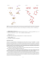
Two examples of successful matings are shown in Figure 1.
Only four keywords affect the mating algorithm:
mating_probability int:1
The probability method used in the selection process of the parents from the population. The probability pi
for each parent i, which has energy Ei is proportional to the following expressions, where Emin is the lowest
energy in the population and Emax the highest:
1 Boltzmann pi = e
Ei −Emin
Em
2 Linear ranges pi = 1.0 −
, with Em determined by the mating_energy keyword
Ei −Emin
Emax −Emin +nEmin ,
with n = number of candidates in the population
3 Equal ranges pi = 1.0
10
parent 1
parent 2
rotated
parent 1
rotated
parent 2
rotated
rotated
transfer
transfer
child
child
Figure 1: Two examples of matings. On the left for Si4 Li, where two Si atomic fragments from parent 2 are transferred to
parent 1 and positioned in the final child so as to avoid interatomic distances that are too small. On the right hand side,
three water molecules are transferred in a (H2 O)5 cluster. All images are viewed along y with the z axis pointing up.
mating_energy float:-1.0
A parameter used in the Boltzmann distribution based mate selection (i.e., mating_probability 1). If
< 0, the Em used will be Em = Emax − Emin , otherwise it will be used as is.
mating_max int:3
The amount of times that mating is attempted before it is considered to have failed.
mating_rebuild int:1
If ̸= 0 performs a 3D build if a mating fails.
Mutation procedure
Mutation of a single candidate is not implemented for several reasons. In our type of candidates, i.e., unique
geometries representing minima on a multidimensional potential energy surface, a mutation is a geometry
modification of fragments and/or atoms in such a way that the mutation is still a candidate that a computational
program can work with. This means that care needs to be taken to not create inter atomic distances that are
too small, which is not a trivial requirement for three dimensional structures with possibly a large amount of
atoms. Thus the first reason is to keep complexity down.
Secondly, the computational program optimizes all atomic positions which effectively are already mutations of atomic positions, but admittedly not random ones.
Thirdly, a form of mutation is inherent in the mating methodology by virtue of the random rotation of the
parents in the procedure. Even when mating the same parents multiple times, different children will result,
thus a set of children from the two same parents will be different just as if a mutation was applied.
Finally, it also bears pointing out that in a system with molecular fragments, due to the geometry optimization of the candidates, not only the relative positions of the fragment centers themselves changes but also the
relative atomic positions within the fragment. This can be considered a mutation of the fragments themselves,
which may be used in future mating procedures.
11
3.8
Termination
As described above, the cluster program will build, or rebuild, an initial population that will be used as a
source of parents for the creation of a single child, which will be optimized, in each mating cycle.
Two keywords are available that can be used to terminate the main cycle of matings. Whenever one of
them is met, the program will exit.
matings int:1
The maximum number of matings attempted.
unchanged int:0
The maximum number of consecutive times that the population is allowed not to be changed by the mating
cycles. If set to a value ≤ 0, this parameter will not affect termination.
4
File Formats
In order to provide flexibility in the workings of the program, several types of files will be created or interpreted. The notation for the file formats description uses [] for optional contents and {} for a repetition of
0 or more items between the {}. If the {} is followed by a symbol that symbol refers to the number of times
this item is expected. The symbol | separates different options of which one should be present.
4.1
Computational program templates
The cluster program uses hard-coded python strings with placeholders to generate input files for the computational programs it interfaces with. To provide more flexibility in the complexity of the input files, it is
possible to have the cluster program read template strings from files in the working directory.
If method is set to template, the template files with
.Opt
for a geometry optimization
.Restart for a restart of a geometry optimization using force constants
.Freq
for a frequency analysis/Hessian calculation
concatenated to the program may be needed. The restart and frequency calculation runs can expect the cluster
program to have kept the restart information needed. If the required template files are not found in the current
working directory the program will create them and exit.
If one needs the extra flexibility that the use of templates provides, it is advised to first have the cluster
program generate the template files that the implemented interface in the cluster program requires. This can
be done by not having any template files in the folder as the cluster program is executed with the method
keyword set to template. The template files created may then be modified as needed and will be used in
future runs of the cluster program in that folder, see also Section 6.8.
A template file should be a properly formatted input file and may have the following placeholders for the
parameters, see also Sections 3.1 and 3.3:
%(xyz)s
%(charge)d
%(multiplicity)d
%(spin_polarization)d
%(method)s
%(processors)d
%(memory)d
%(max_scf)d
%(max_opt)d
%(root)s
%(rootpath)s
the cartesian coordinate block for optimization.
the charge of the candidate.
the multiplicity of the candidate 2S + 1.
the number of unpaired electrons 2S.
the computational method (and basis set etc) to be used.
the number of processors.
the amount of memory (in MB).
the maximum number of SCF cycles.
the maximum number of geometry optimization steps.
will be the name of the candidate.
will be the OUT_DIR path with the name of the candidate appended.
If one keeps the %(method)s placeholder in the template file, the default method for the particular program
will be used.
12
4.2
Element library and elements format
The element radii in the library of predefined elements are taken from the WebElements web site. 12 They are
read from a file in the cluster program’s library folder (lib/elements.dat). In order to provide more
flexibility, it is also possible to read a new definitions from a user specified files or by defining elements
directly in the input file. The file format is a sequence of one-liners defining an element or a comment:
{[comment_line | element_line]}
comment_line: # {string}
element_line: [string:key] string:element_name int:Z float:radius
The radius is in Å. If the key string is omitted, element_name will be used as the key. If the key string is
present, as in the examples below, any text after the radius will be ignored.
The key is the string that needs to be used in fragment element names and/or in the composition string of
candidates. One can define atomic ions as if it were an element, e.g., F− and Hg2+ with the lines
FF
9 1.2
Hg2+ Hg 80 0.7
# larger than the 0.71 Angstrom in the built-in library
# smaller than the 1.49 Angstrom in the built-in library
and use it in the composition or in fragment definition(s).
4.3
Fragment library and fragments format
The predefined library of fragments, located in in the library folder of the cluster program (lib/fragments.xyz), consists of optimized geometries calculated with ORCA using PBE/TZVPP and VDW06. In
order to provide more flexibility it is also possible to read fragments from user specified files. The file formats consists of a concatenation single fragment descriptions, each of which is xyz-file formatted 5 with the
modification that in that the comment line has specific information encoded. i.e., the fragment library format
is as follows:
{ int:natoms
string:name float:radius {string}
{ string:elementkey float:x float:y float:z
}natoms }
The name is the string needed in the composition string of candidates, while radius is an additional radius,
in Å, used in building candidates and genetic operations, see Sections 3.4 and 3.7.
The elementkey in an xyz-file is the element name. The cluster program allows a bit more flexibility
because the key is the key for the element in the element library, which may differ from the actual element
name, thus it is possible to use the following fragment definition as long as the Hg2+ and F- ’elements’ are
defined, see Section 4.2:
3
HgF2 1.0
Hg2+ 0 0
F- -2 0
F2 0
4.4
just a silly example
0
0
0
Candidate library format
The file format for a library of candidates is also a slightly modified version of the standard multistep xyz
file format, in that the comment line has specific information encoded for the name, energy (E), nuclear
repulsion energy (R) and lowest vibrational frequency (freq) followed by an optional comment. If the energy
and/or frequency are not computed, the float strings inf and -inf are used, respectively. The file format
for a cluster library is as follows:
{ int:natoms
string:name float:E float:R float:freq {string}
{ string:elementname float:x float:y float:z
}natoms }
13
5
Computational program interfaces and examples
This sections provides some information regarding the implementation of the interface to specific computational packages. It is strongly recommended to check out the example inputs for the ADF program, even if
one doesn’t have that available, because it shows some more advanced use of some of the available features
in the cluster program.
5.1
ADF
Requirements
The ADFBIN environment variable needs to be defined, as well as the adfrc.sh or adfrc.csh should have been
sourced because the cluster program calls the ADF program by using $ADFBIN/adf with the command line
option -n set to the number of processors requested in the cluster input file.
Defaults
The default method for ADF calculations uses the LDA SCF VWN functional with a TZP basis set and a large
core. The default geometry optimization criterion for the energy is tightened to 1e-4 from the more permissive
1e-3 hartree.
Specifics
• The ADF program requires the method of calculation and basis set to be provided in blocks containing
multiple lines. As a result of that \n is needed in the method keyword unless one decides to use the
template value. Note that the former can lead to a very long single line for this keyword.
• ADF expects in the input the number of unpaired electrons as opposed to the spin multiplicity, so the
cluster program will determine the number of unpaired electrons from the multiplicity setting and uses
%(spin_polarization)d in the template file to do so.
• For the frequency analysis calculation, the default is to use analytical frequencies, so a user has to use
templates for functionals where analytical frequencies are not available.
• The default frequency calculation template also contains ScanFreq -1000 0 for recalculating
the imaginary frequencies. The cluster program will replace the initially calculated frequency values
as reported in the regular ”Vibrational and Normal Modes” table with the new value from the scan
frequencies output section for all vibrations whose ’old’ frequency is within 0.01 cm−1 of the initial
value, so that all frequency values for degenerate modes are replaced.
• The memory placeholder is not used in the templates.
• The energy value is taken from the regular expression match of every line in the output file with:
r’Total Bonding Energy:.*?([-+0-9.]+)’
ADF Example 1
The example below is for an unrestricted calculation which requires a quite lengthy method line in the input
to achieve this. Only a small amount of the default values of the keywords may need to be reassigned. In this
case that has been kept to a minimum.
name
Si4Li
#
# Note the method argument should be a single long string, the split over two
# lines should not be in the real input file
#
program
ADF
method
XC\nGGA BLYP\nEND\nBASIS\ntype TZP\ncore Large\nEND\nUNRESTRICTED
processors 8
multiplicity 2
14
charge
composition
1D
2D
3D
matings
0
Si 4 Li 1
2
5
10
40
energy_resolution
5e-4
repulsion_resolution 2
ADF Example 2
This example shows how the definition of a fragment can be done by using the fragments keyword. With
only three fragments in the cluster it is not really necessary to generate 3D candidates since the centers of
three fragments are always in a 2D plane, thus the default of not creating 3D candidates is kept in place.
In this particular case the nfreq_cutoff is set to a negative value, because earlier runs showed that
it was hard to get structures without slightly negative frequencies after the initial build. A filter run, see
ADF Example 3, can be performed later to get rid of these.
name
3xCaI2
program
method
processors
ADF
XC\nGGA BLYP\nEND\n\nBASIS\ntype TZP\ncore Large\nEND
8
multiplicity
charge
composition
1
0
CaI2 3
1D
2D
matings
2
10
40
nfreq_cutoff -5.0
energy_resolution
5e-4
repulsion_resolution 4
fragments
3
CaI2 0.0
Ca 0.0 0.0 0.0
I
0.0 0.0 2.8316
I
0.0 0.0 -2.8316
ADF Example 3
An example of a filter utility run, where now the candidates with negative frequencies are removed from
the viable population, keeping the original file intact, but generating the newly filtered population in the file
3xCaI2_flt.xyz as well as the associated .csv file. The repulsion resolution has been set to a bit more
lenient value, as well.
name
filter
energy_resolution
repulsion_resolution
3xCaI2
flt
5e-4
10
15
5.2
g09/g03
Requirements
The gaussian interfaces for g09 and g03 require that the gaussian root environment variables, g09root or
g03root, are defined as well as that their respective .login files have been sourced, i.e., the normal gaussian
setup has been performed, because the cluster programs executes either g03 or g09 directly.
Defaults
The default method for gaussian calculations is B3LYP/3-21G.
Specifics
• The g09 and g03 program interfaces are the same with respect to input file create and output file parsing.
The only differences are in how the program is called, and that the g03 program limits the number of
processors to 8.
• Because the text used to report the energy is not the same for the different methods that Gaussian
supports, several regular expression patterns are used when matching the lines from the output file.
The last match encountered will be the energy that the cluster program reports and uses for comparison.
The list of patterns and the type of calculation it matches are as follows:
EpatSearch = [
re.compile(r’SCF Done:.*?=.*?([-+0-9.eED]+)’),
re.compile(r’E\(CORR\)=.*?([-+0-9.eED]+)’),
re.compile(r’E[UR]MP.*?=.*?([-+0-9.eED]+)’),
re.compile(r’[UR]MP4.*?=.*?([-+0-9.eED]+)’),
re.compile(r’E\(CI\)=.*?([-+0-9.eED]+)’),
re.compile(r’E\(.*2PLYP\).*?=.*?([-+0-9.eED]+)’),
re.compile(r’CBS-.*\(0 K\)=.*?([-+0-9.eED]+)’),
re.compile(r’\s*Energy=.*?([-+0-9.eED]+).*?NIter’)
]
#
#
#
#
#
#
#
#
SE(g09), HF, DFT
CCx and QCI*
MP2/3 and CIS
MP4
CISD
*2PLYP
CBS-*
SE from g03
g09 Example
A similar example as the ADF Si4 Li one, but now for Si4 Li3 using Gaussian’s g09 (the only modification to
use g03 is to change g09 in the program line to g03. Note that since g03 and g09 automatically change a
calculation to an unrestricted one when the multiplicity is not 1, we do not have to stipulate UB3LYP, but we
could.
For clarity the maximum number of optimization and SCF cycles have been explicitly defined.
name
Si4Li3
program
method
processors
memory
max_opt
max_scf
g09
B3LYP/SDD
8
6000
50
50
multiplicity 2
charge
0
composition Si 4 Li 3
1D
2D
3D
matings
2
5
10
40
16
energy_resolution
5e-4
repulsion_resolution 2
5.3
ORCA
Requirements
The ORCA environment variable should be defined as the folder containing the ORCA executable which
should also be in the path because the cluster program calls $ORCA/orca directly.
Defaults
The default method in the template for ORCA is RKS B3LYP/G SV.
Specifics
• The energy value is taken from the regular expression match of every line in the output file with:
r’FINAL SINGLE POINT ENERGY.*?([-0-9.]+)’
ORCA Example
A Li4 cluster using ORCA.
name
Li4
program
method
processors
memory
ORCA
RHF SV
1
200
multiplicity
composition
charge
1
Li 4
0
1D 1
2D 1
3D 1
restart
matings
5.4
0
5
# force to start from scratch
MOPAC
Requirements
The MOPAC environment variable should be set to the full path of the MOPAC executable (.exe) file, since
the cluster program executes ${MOPAC} directly.
Defaults
The default method is PM7
17
Specifics
• Since MOPAC does not write output to the standard output stream, it can not be redirected to be appended to an earlier output in the program call itself. Thus the final output file for a viable candidate
only consists of the latest, i.e., frequency, calculation.
• Since it wasn’t clear how to restart an optimization using the Hessian from an earlier frequency calculations, the reoptimization part is not implemented in the candidate optimization cycle, so only multiple
starts of optimizations will be performed up to max_freq times.
• The default max_opt may be too small. Since MOPAC is quite fast, it doesn’t hurt to make max_opt
a lot larger.
• Consider using PRECISE after the method as well, e.g., PM7 PRECISE. This will tighten convergence
criteria for the optimizations.
• MOPAC reports the heat of formation energy in kcal/mol, which the cluster program converts to hartree
units.
• the memory and processors are not used in the templates.
• Because the optimization and the frequency calculation report energies slightly differently, two regular
expression patterns are used when matching the lines from the output file. The last match encountered
will be the energy that the cluster program reports and uses for comparison. The two patterns are:
r’HEAT OF FORMATION.*?=.*?([-+0-9.eE]+)’
r’HEAT:.*?([-+0-9.eE]+)’
MOPAC Example
A water pentamer cluster, (H2 O)5 calculation using the PM3 method with the PRECISE keyword. Note that
the maximum number of optimization cycles allowed is increased by quite a bit from the standard 50. This
example also forces the calculation to start from scratch, i.e., any previously calculated results found in the
work folder will be deleted.
name
program
method
max_opt
w5
MOPAC
PM3 PRECISE
500
composition H2O 5
charge
0
multiplicity 1
restart
2D
3D
matings
0
20
40
50
repulsion_resolution 1
5.5
ADFUFF
The default implementation of the UFF program by ADF may not work too well because the cluster program
only generates the coordinates of the input structures and not the atom types nor bonds. The interface was
written because a user can, by using input templates, have UFF use the user’s atom type database (for automatic
atom type assignment) and force field parameters for those atom types.
One can also consider using the ADFUFF program to generate an initial population that in a subsequent
run with a different program can be made to be optimized using a better methodology (see reoptimize).
18
Requirements
Just like for the ADF interface, the ADFBIN environment variable needs to be defined, as well as the adfrc.sh or adfrc.csh should have been sourced because the cluster program calls ADF’s UFF program by using
$ADFBIN/uff with the command line option -n set to the number of processors requested in the cluster
input file.
Defaults
Since this is an MD type program, no method needs to be specified
Specifics
• Since one can not restart an optimization using the Hessian from an earlier frequency calculations, the
reoptimization part is not implemented in the candidate optimization cycle. Only multiple starts of
optimizations will be performed up to max_freq times.
• Only the max_opt keyword is used in the templates. But the charge and multiplicity must be
set appropriately since the multiplicity value is tested against what is possible based on the number of
electrons in the system.
ADFUFF Example
A water tetramer cluster, (H2 O)4 . Since the default mechanism for associating atom types in the structure is
completely based on the automatically determined bond connectivity, this run generates some strange structures.
name
H2O_4
program ADFUFF
multiplicity 1
charge
0
composition H2O_L 4
nfreq_cutoff
restart
2D
3D
matings
-10
0
5
30
50
repulsion_resolution 0.2
5.6
EFPMD
Requirements
The EFPMD environment variable should be set to the full path of the efpmd executable file, since the cluster
program executes ${EFPMD} directly.
Defaults
Since this is an MD type program, no method needs to be specified
19
Specifics
• Since one can not restart an optimization using the Hessian from an earlier frequency calculations, the
reoptimization part is not implemented in the candidate optimization cycle. Only multiple starts of
optimizations will be performed up to max_freq times.
• Since EFPMD treats fragments as a whole, the hessian is not calculated on a per atom basis. This means
that calculated displacement vectors from the frequency calculation can not be used to displace atomic
coordinates and the cluster program will not be able to move away from a maximum so local maxima
are immediately aborted.
• EPFMD often shows small negative frequencies in its minima, so set nfreq_cutoff to a negative
value.
• Only the max_opt keyword is used in the templates. But the charge and multiplicity must be
set appropriately since the multiplicity value is tested against what is possible based on the number of
electrons in the system.
• If one wants to use libEFP library fragments, the fragment name with _L should also be defined in
the library files that the cluster program parses. The sequence of the atom types in the two fragments
should be the same. Currently the libEPF fragments distributed with 1.2.1 are part of the cluster known
fragments.
EFPMD Example
A water tetramer cluster, (H2 O)4 . Because of issues with the normal mode analysis not being atom but
fragment based (see above) and often having small negative frequencies, the nfreq_cutoff is set to a
largish negative value (one could even use -inf to accept all stationary points). The fragment name is
H2O_L so that the libEFP program will use it’s own H2O fragment.
name
H2O_4
program EFPMD
multiplicity 1
charge
0
composition H2O_L 4
nfreq_cutoff
restart
2D
3D
matings
-10
0
5
30
50
repulsion_resolution 0.2
6
Cluster usage examples
This section shows some examples on approaches of using the cluster program. The input and output files are
stored in the examples folder provided.
6.1
Testing input
To test an input file that will be used later with the computational method planned, a test run calculation may
be performed. The input file, shown below and available in the examples/H2S/test folder, has already
the planned build, mating and acceptance keywords, but since it contains the line test 1, only a single test
of the program templates available will be executed. Note that in this case the definition of H2 S is stored
externally in the H2S folder’s fragments.xyz file, since it is not a fragment in the standard library and we
will be using it a few times in these examples.
20
name H2S
test 1
program MOPAC
method PM7 PRECISE
charge
multiplicity
composition
1D
2D
3D
matings
0
1
H2S 3
2
5
20
30
energy_resolution 5e-4
repulsion_resolution 2
fragmentlib ../fragments.xyz
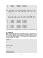
After executing the cluster program with this input file, the folder will contain the input and output files for
each of the test runs using the name test_3D as the root name for the 3D build candidate that is generated.
The resulting output from the cluster program itself, which was redirected to the test.out file, shows that
the prototype of the trimer indeed uses 3 H2S fragments from the fragment library which have an extra radius
of 0.3 Å:
###################### LIBRARIES READ WHILE PARSING INPUT ######################
fragmentlib ../fragments.xyz
############################## BUILDING PROTOTYPE ##############################
3 x H2S (extra radius 0.300 Angstrom):
H
0.2863440033
0.0647336800
-0.9761714367
H
-0.4595735367
-0.6015626800
0.6826481633
S
0.1732295333
0.5368290000
0.2935232733
For an overall composition of (H2S)3.
Having 9 atoms and 54 electrons.
############################### PROGRAM SETTINGS ###############################
Below that, a one-liner result of the optimization and frequency runs are given each followed with the
cluster library entry for the candidate after the computational program finished. No ReOpt run is performed
since the MOPAC interface does not support this. Inspection of the Opt and Freq output lines shows that
no error codes are returned, the None values. More importantly, the geometry optimization was not able to
converge in the default 50 optimization cycles allowed. Since the MOPAC interface only supports running
several direct optimizations in a row, without a frequency analysis and reoptimization in between, we should
increase the max_opt.
The frequency calculation does indeed give us frequencies, which suggests that that calculation works as
it should. Note that even though it has converged=True in the information about the Freq calculation, one
does not have to worry about this, because the cluster program will retain the information about the geometry
convergence from the earlier geometry (re)optimization(s).
##################### TEST INPUT FILES FOR A 3D CANDIDATE ######################
Opt: (None) code=None E=-2.169030E-02 converged=False failed=False Freq:[]
9
test_3D -0.021690302 154.932 -inf Build 3D scale=1
H
1.1518252540
-2.1202304363
0.4178235809
H
-0.1886989782
-3.6200137545
0.4001815406
S
-0.0961472187
-2.3469205038
-0.0118190440
H
1.2367631676
1.3648574145
0.1764851672
21
H
S
H
H
S
2.8606317737
2.5485261164
-3.0582649197
-2.4364364714
-2.0181987237
2.0233658701
1.0962064923
1.9205378907
0.2065601384
1.4756368884
-0.8145101256
0.0990490047
-0.6013266369
0.2210352951
0.1130812179
Freq: (None) code=None E=-2.171221E-02 converged=True failed=False Freq:[(-533.2,
[0.0076, 0.0021, -0.0222, 0.0066, 0.0142, 0.0031, 0.0084, 0.0502, -0.0221]),
(-89.8, [-0.0059, 0.0083, 0.0471, -0.0056, -0.0, 0.0153, -0.0119, 0.0222,
0.0304]), (-81.5, [0.1259, -0.0057, -0.1394, 0.1259, 0.0188, -0.0139, 0.6485,
0.0363, 0.0101]), (-46.7, [0.0273, -0.0498, -0.5469, 0.0263, 0.0737,
-0.0733, -0.1545, 0.0711, 0.1189]), (-38.3, [-0.1771, 0.2375, 0.6545,
-0.1718, -0.1934, 0.0836, 0.0885, 0.1109, -0.1303]), (32.8, [0.0514, -0.0973,
0.0505, 0.0517, -0.0882, 0.0656, 0.268, -0.524, 0.3122]), (51.8, [0.1213,
-0.116, -0.0834, 0.1202, 0.17, -0.0366, -0.0292, 0.1557, -0.0408]), (92.3,
[0.3474, -0.4314, 0.3077, 0.3456, 0.4123, 0.4505, -0.1408, -0.0505, -0.1607])
]
9
test_3D -0.021712211 154.932 -533.20 Build 3D scale=1
H
1.1518252540
-2.1202304363
0.4178235809
H
-0.1886989782
-3.6200137545
0.4001815406
S
-0.0961472187
-2.3469205038
-0.0118190440
H
1.2367631676
1.3648574145
0.1764851672
H
2.8606317737
2.0233658701
-0.8145101256
S
2.5485261164
1.0962064923
0.0990490047
H
-3.0582649197
1.9205378907
-0.6013266369
H
-2.4364364714
0.2065601384
0.2210352951
S
-2.0181987237
1.4756368884
0.1130812179
##################################### DONE #####################################
Thus we can use the cluster input file, but with a larger number of geometry cycles for production runs, and
with the test 1 removed or commented out.
6.2
Multiple runs
It may be beneficial to run the same cluster search multiple times and refilter the viable or population candidates found from all runs combined. This is most easily done by running each input in its own folder. It
may be useful to make sure that the name keyword contains something that allows one to retrace which run
generated a particular candidate, while keeping the rest of the input the same. In the examples/H2S folder,
this is done in the folders r1, r2, r3, r4, and r5.
The input file in the r1 folder, r1.in, is as follows:
name H2S_r1
program MOPAC
method PM7 PRECISE
max_opt 500
charge
multiplicity
composition
1D
2D
3D
matings
0
1
H2S 3
2
5
20
30
energy_resolution 5e-4
repulsion_resolution 2
22
fragmentlib ../fragments.xyz
When the cluster runs are finished, one may quickly see which runs generated which candidates in the populations by using grep (on LINUX/UNIX type systems only...)
rkanters:H2S rkanters$ grep _ r*/*pop*.xyz
r1/H2S_r1_population.xyz:H2S_r1_4 -0.023556492 163.663 28.80 Build 2D scale=1
r1/H2S_r1_population.xyz:H2S_r1_18 -0.021987541 144.368 3.40 Build 3D scale=1
r2/H2S_r2_population.xyz:H2S_r2_1 -0.021989498 145.184 3.10 Build 1D scale=1
r2/H2S_r2_population.xyz:H2S_r2_43 -0.015519401 194.769 18.50 H2S_r2_4 x H2S_r2_4
r2/H2S_r2_population.xyz:H2S_r2_4 -0.012641140 180.537 13.10 Build 2D scale=1
r3/H2S_r3_population.xyz:H2S_r3_4 -0.023558056 163.867 17.70 Build 2D scale=1
r3/H2S_r3_population.xyz:H2S_r3_13 -0.022450474 159.517 22.30 Build 3D scale=1
r3/H2S_r3_population.xyz:H2S_r3_1 -0.021960593 142.241 4.70 Build 1D scale=1
r4/H2S_r4_population.xyz:H2S_r4_6 -0.022375850 160.280 31.90 Build 2D scale=1
r5/H2S_r5_population.xyz:H2S_r5_4 -0.021980137 143.607 5.50 Build 2D scale=1
And it is immediately clear that in most runs the candidates were found during the build stage, and not the
mating cycles.
Since the population library is a subset of the viable library we will combine the viable libraries of all runs
into a an all_viable.xyz library file in the examples/H2S/all folder, wherein is executed with the
idea that any filter utility run using name all will be working with the library:
cat ../r*/*via*.xyz >all_viable.xyz
The all_viable.xyz viable library can now be used for sorting and/or refiltering as described next.
6.3
Sorting and refiltering libraries
Since the viable library does not store the candidates sorted by energy it may be useful to perform a filter
utility run that will only sort, not actually filter, it to create a new population library that contains all the
viable candidates sorted by energy. Inspecting the resulting library, or inspecting the text output, may help in
determining the repulsion and energy resolution values one should use to filter out only the unique structures
in a subsequent run.
To sort the viable library all one needs is a simple filter input file, which is in the examples/H2S/all
folder called sort_via.in. By turning all energy acceptance criteria off, every structure in the all_viable.xyz
will be considered unique. Since the original viable libraries contained candidates with positive frequencies,
we can keep the frequency based filter to its default settings:
name all
filter sorted
energy_resolution -1
repulsion_resolution -1
energy_window -1
Since the filter procedure only parses the comment lines in the xyz files, no composition information is needed.
The text output it generates shows that indeed no duplicates are taken from the new filtered set of structures:
############################ DUPLICATES IN VIABLES #############################
############################# FILTERED POPULATION ##############################
H2S_r3_4: Filtered
E = -0.023558056 R = 163.867 v = 17.70
H2S_r1_4: Filtered
E = -0.023556492 R = 163.663 v = 28.80
H2S_r1_3: Filtered
E = -0.023555334 R = 163.507 v = 26.70
H2S_r3_13: Filtered
E = -0.022450474 R = 159.517 v = 22.30
H2S_r4_6: Filtered
E = -0.022375850 R = 160.280 v = 31.90
H2S_r2_1: Filtered
E = -0.021989498 R = 145.184 v = 3.10
H2S_r1_18: Filtered
E = -0.021987541 R = 144.368 v = 3.40
23
H2S_r5_4: Filtered
H2S_r5_2: Filtered
H2S_r1_1: Filtered
H2S_r3_1: Filtered
H2S_r2_43: Filtered
H2S_r2_4: Filtered
E
E
E
E
=
=
=
=
-0.021980137 R = 143.607 v = 5.50
-0.021979759 R = 143.056 v = 3.70
-0.021974507 R = 142.948 v = 6.20
-0.021960593 R = 142.241 v = 4.70
E = -0.015519401 R = 194.769 v = 18.50
E = -0.012641140 R = 180.537 v = 13.10
One may double-check by visualizing the structures in the all_sorted.xyz file using Jmol, or any
other visualization program that can deal with multi-step xyz files, to see which candidates do indeed look
similar enough to be considered duplicates. An energy resolution of 0.0001 and a very generous repulsion
resolution of 2 will filter several duplicates out, as shown in the flt.out, which is the result of using the
flt.in input file.
############################ DUPLICATES IN VIABLES #############################
H2S_r1_4: == H2S_r3_4
E = -0.023556492 R = 163.663 v = 28.80
H2S_r1_3: == H2S_r3_4
E = -0.023555334 R = 163.507 v = 26.70
H2S_r4_6: == H2S_r3_13
E = -0.022375850 R = 160.280 v = 31.90
H2S_r1_18: == H2S_r2_1
E = -0.021987541 R = 144.368 v = 3.40
H2S_r5_4: == H2S_r2_1
E = -0.021980137 R = 143.607 v = 5.50
H2S_r1_1: == H2S_r5_2
E = -0.021974507 R = 142.948 v = 6.20
H2S_r3_1: == H2S_r5_2
E = -0.021960593 R = 142.241 v = 4.70
############################# FILTERED POPULATION ##############################
H2S_r3_4: Filtered
E = -0.023558056 R = 163.867 v = 17.70
H2S_r3_13: Filtered
E = -0.022450474 R = 159.517 v = 22.30
H2S_r2_1: Filtered
E = -0.021989498 R = 145.184 v = 3.10
H2S_r5_2: Filtered
E = -0.021979759 R = 143.056 v = 3.70
H2S_r2_43: Filtered
E = -0.015519401 R = 194.769 v = 18.50
H2S_r2_4: Filtered
E = -0.012641140 R = 180.537 v = 13.10
Note that H2S_r2_1 and H2S_r5_2 have very similar energies, but their nuclear repulsion resolutions
are quite different, suggesting that they may be different structures.
Keep in mind that since no new optimizations are performed, none of this will find any candidates that were
considered duplicates during the initial runs but not according to the new criteria, i.e., setting the duplicate
detection criterion settings tighter than what was used in the initial runs will not increase the number of
candidates in the resulting population library. Thus if one thinks that the initial input file that created the
viable library contained too generous duplicate determination criteria, one should inspect the duplicate library
for the runs, to see whether a restart could be in order.
Of course one may want to consider sorting without any filtering, i.e., also allowing negative frequencies in
the candidates, but doing that with the converged library as opposed to the viable library. This allows one to see
whether there are low energy maxima that had problems optimizing to a lower energy structure, suggesting that
an actual minimum that should be present was not found. For instance in the examples/H2S/converged
folder one may execute
cat ../r*/*conv*.xyz >conv_viable.xyz
And use the following input file to only sort the candidates leaving candidates with negative frequencies in
the mix by using -inf for the frequency cutoff, as shown in conv_sorted.in:
name conv
filter sorted
energy_resolution -1
repulsion_resolution -1
energy_window -1
nfreq_cutoff -inf
The start of the filtered population that this gives shows that the frequency calculation may be problematic for
the lowest energy candidates listed here, even though they really are practically the same structures (based on
inspection of the generated population library):
24
############################ DUPLICATES IN VIABLES #############################
############################# FILTERED POPULATION ##############################
H2S_r2_3: Filtered
E = -0.023558996 R = 163.685 v = -759.80
H2S_r3_28: Filtered
E = -0.023558354 R = 163.576 v = -369.30
H2S_r3_4: Filtered
E = -0.023558056 R = 163.867 v = 17.70
H2S_r5_3: Filtered
E = -0.023557837 R = 163.538 v = -731.20
H2S_r4_3: Filtered
E = -0.023557507 R = 163.550 v = -738.60
H2S_r1_5: Filtered
E = -0.023556889 R = 163.536 v = -96.90
H2S_r1_4: Filtered
E = -0.023556492 R = 163.663 v = 28.80
H2S_r1_3: Filtered
E = -0.023555334 R = 163.507 v = 26.70
....
6.4
Reoptimizing a library
A library like the one created in the examples/H2S/all folder may be used as the initial population for
a reoptimization using another program, e.g., ADF. The files for the ADF cluster run are stored in the examples/H2S/ADF folder. First we will copy the filtered library into the ADF folder. Since we will use the
name H2S_ADF, the population file that will be reoptimized is called H2S_ADF_population.xyz. Because the cluster program will overwrite the population library file, we will keep a copy called initial.xyz
around in case we need to redo this part.
rkanters:ADF rkanters$ cp -p ../all/all_flt.xyz initial.xyz
rkanters:ADF rkanters$ cp initial.xyz H2S_ADF_population.xyz
The input file for the cluster run itself should now specifically state that a reoptimization should be done.
It is important that the composition string is exactly the same as the one used to generate the libraries
since it affects the sequence in which atoms are expected to be found in the xyz file formats. The input file
listed below is to be run on a computational cluster where the programs are executed in a temporary folder and
not within the current working directory. This means that one has to use the full path for fragmentlib (or
elementlib) which should be on a file system that all compute nodes have access to. Thus H2S_ADF.in
looks like:
name H2S_ADF
program
method
processors
memory
ADF
XC\nLDA SCF VWN\nEND\n\nBASIS\ntype TZP\ncore Large\nEND
8
6000
multiplicity 1
charge
0
composition
H2S 3
reoptimize
matings
1
0
energy_resolution -1
repulsion_resolution -1
energy_window -1
fragmentlib /home/rkanters/work/cluster/H2S/fragments.xyz
Just for illustrative reasons the cluster program is to not filter out any optimized geometries based on the
energies by turning off all energy related acceptance criteria. Normally one would have a reasonable idea
about the criteria to use and avoid unnecessary frequency calculations. Also no matings are requested since
we only want to reoptimize the population library.
25
At the end of the cluster output we see that four of the six candidates are reoptimized to basically the same
structure. From the inspection of the H2S_ADF_population.csv file it is clear just how close the first
four structures are in energy, i.e., within 0.011 kcal/mol and a range of the repulsion resolutions of about 0.6
hartree:
name,E/Eh,dE/Eh,dE/eV,dE/(kcal/mol),R/Eh,Freq/cm-1,comment
H2S_ADF_3,-1.280270003,0.000000000,0.000000000,0.000000,183.440,124.91,”
Population H2S_r2_1”
H2S_ADF_1,-1.280264632,0.000005371,0.000146155,0.003370,183.708,127.36,”
Population H2S_r3_4”
H2S_ADF_2,-1.280255768,0.000014235,0.000387342,0.008932,183.184,125.34,”
Population H2S_r3_13”
H2S_ADF_4,-1.280252325,0.000017677,0.000481028,0.011093,183.530,125.93,”
Population H2S_r5_2”
H2S_ADF_5p,-1.280045216,0.000224787,0.006116765,0.141056,183.402,119.34,”
Population H2S_r2_43”
H2S_ADF_5n,-1.274771463,0.005498540,0.149622877,3.450386,183.227,72.85,”
Population H2S_r2_43”
H2S_ADF_6,-1.267672306,0.012597697,0.342800768,7.905174,160.478,12.37,”Population
H2S_r2_4”
Thus we really wasted some time calculating the frequencies for candidates 2 and 4 (1 would always be
calculated and since 3 ends up with a slightly lower energy, it would be calculated as well). Inspection of
the population library shows that within the four lowest energy structures contain non-superimposable mirror
images, which even a slight filtering would have considered duplicates.
It is interesting to note that here we see a case where the bifurcation results in two different candidates
in the population, i.e., H2S_ADF_5p and H2S_ADF_5n both are the result from the optimization of the
H2S_r2_43 candidate from the initial population, as can be gleaned from the comment for each candidate.
6.5
Seeding the population library
Due to the randomness in the build and mating procedures, one is not guaranteed to get the same populations
every time a cluster job is run. If you executed the previous steps in finding a library of (H2 S)3 molecules, it
is likely that you would indeed get the same lowest energy structure(s), but when I executed the same set of
runs before I did not encounter the trimer in which all three dangling H’s are on the same side of the ring of S
atoms. To make sure that the program will consider this candidate, we will seed the initial population with a
duplicate of the lowest energy structure encountered, but with the one H on the first H2 S moved to the other
side. We will also remove the other candidates from the file. This edited population library will be used in
another ADF calculation, this time stored in the examples/H2S/ADF2 folder. We also need to flag that
the second one needs optimization. The initial population file to be used now looks like (note the inf in the
second structure as well as the change in the z coordinate of the first hydrogen is changed to -1.15):
9
H2S_ADF_3 -1.280270003 183.440 124.91 Population H2S_r2_1
H
-1.8611392375
1.1350155879
1.3998146899
H
-0.3947405456
1.3078773930
0.1021772479
S
-1.7780389666
1.1034449824
0.0433127875
H
1.8784401317
1.0099340188
-1.1544075407
H
1.3354105540
-0.3046479439
0.2052837443
S
1.8510702418
0.9959604779
0.2046679226
H
-0.9318295376
-0.9915431837
0.1432715487
H
-0.0384564056
-2.1715810038
-1.1502910739
S
-0.0607162347
-2.0844603286
0.2061706737
9
ignored inf
H
-1.8611392375
1.1350155879
-1.15
H
-0.3947405456
1.3078773930
0.1021772479
S
-1.7780389666
1.1034449824
0.0433127875
26
H
H
S
H
H
S
1.8784401317
1.3354105540
1.8510702418
-0.9318295376
-0.0384564056
-0.0607162347
1.0099340188
-0.3046479439
0.9959604779
-0.9915431837
-2.1715810038
-2.0844603286
-1.1544075407
0.2052837443
0.2046679226
0.1432715487
-1.1502910739
0.2061706737
The input file should not request a reoptimization, since H2S_ADF_3 is still OK. A regular restart will detect
the inf for the energy of the second candidate, which we called ignored, and reoptimize only this candidate.
The input file looks the same as the earlier reoptimization one, just without the reoptimization line itself:
name H2S_ADF
program
method
processors
memory
ADF
XC\nLDA SCF VWN\nEND\n\nBASIS\ntype TZP\ncore Large\nEND
8
6000
multiplicity 1
charge
0
composition H2S 3
matings
0
energy_resolution
-1
repulsion_resolution -1
energy_window
-1
fragmentlib /home/rkanters/work/cluster/H2S/fragments.xyz
Since we ran the input in a new folder where only a population library existed and not the all library and
converged library, the newly optimized structure numbers start with 1 above the largest one in the population
library, i.e., 4. The default duplicate checking will start with an empty list of converged structures to check
against. In the output we see that the final population has the new structure optimized and indeed named
H2S_ADF_4:
##################### ALGORITHM END: CONSIDERED 0 MATINGS ######################
The run generated 1 candidate.
############################### FINAL POPULATION ###############################
H2S_ADF_3: population
E = -1.280270003 R = 183.440 v = 124.91
H2S_ADF_4: population
E = -1.280059430 R = 183.484 v = 121.957
################################### TIMINGS ####################################
From the csv file it is easy to see that the energy difference is only 0.135 kcal/mol and the repulsion resolutions
are only 0.044 hartree different, while the comment for it suggests that it came from a reoptimization of the
initial population:
name,E/Eh,dE/Eh,dE/eV,dE/(kcal/mol),R/Eh,Freq/cm-1,comment
H2S_ADF_3,-1.280270003,0.000000000,0.000000000,0.000000,183.440,124.91,”
Population H2S_r2_1”
H2S_ADF_4,-1.280059430,0.000210573,0.005729991,0.132137,183.484,121.96,”Initial”
6.6
No optimization runs
A somewhat peculiar use of the cluster program, but considered a feature, is to use it to only generate a library
of structures that the cluster program would generate without automatically optimizing them. This is achieved
by setting the max_freq to 0, since that flags the program that no frequency calculations are allowed. Since
there is no point in running a geometry optimization because any converged geometry can not be checked
27
to see whether it is at a minimum or maximum in the PES, the program will not even start the optimization
cycles but abort the candidate and append its structure to the aborted library.
An example where this is done to create the library of structures that are built is provided in the examples/noopt folder. The input file also shows the use of in the composition for trying to build an NH3
surrounded by twenty water molecules. The structural information for the two fragments were copied from
the default fragment library, which is stored in the lib folder of the cluster program. In order to not have
the molecules touch, an extra radius of 0.3Å for each fragment is introduced. The value is half of the difference of an H-bond in water (1.7 Å) from which the sum of the H and O radii are subtracted, 0.37 and 0.73Å,
respectively.
name noopt
composition NH3 1 @ H2O 20
charge 0
multiplicity 1
3D 20
matings 0
max_freq 0
fragments
3
H2O 0.3
ORCA ! PBE VDW06 TZVPP PModel TightSCF Opt UseSym
O
0.000000
-0.000000
0.066734
H
0.000000
0.763595
-0.529847
H
0.000000
-0.763595
-0.529847
4
NH3 0.3
ORCA ! PBE VDW06 TZVPP PModel TightSCF Opt UseSym
N
0.000166
-0.079017
0.000004
H
-0.470994
0.317856
0.815661
H
-0.470988
0.317858
-0.815660
H
0.941816
0.317791
-0.000005
The result of running this input is that only a noopt_aborted.xyz file will be created that contains each
structure built.
To generate only the mated structures based on an available population library from a run, which therefor
should be present in the folder, one would only have to change the matings to the number of children to be
created and rely on the default restart settings for the program. Note that since the mated structures would be
appended to the aborted library, one may want to delete that file first.
6.7
Single fragment runs
Since the cluster program is able to follow the PES off a stationary point that is not a minimum, the program
may also be useful to do just optimizations of a structure that consist of a single fragment. An example of the
optimization of an Si4 Li uncharged doublet system, stored in examples/Si4Li uses the Si4Li.in input
file:
name Si4Li
program
ADF
method
XC\nLDA SCF VWN\nEND\nBASIS\ntype TZP\ncore Large\nEND\nUNRESTRICTED
processors 8
fragmentlib
composition
charge
multiplicity
Si4Li.xyz
Si4Li 1
0
2
28
restart 0
1D
1
nfreq_bifurcate 0
matings 0
to only request a single 1D build of the fragment, which really is the whole structure, to be optimized. The
input structure, stored as an external fragment, is a linear structure known to have imaginary frequencies. If
the symmetry of a converged maximum is low, it may be possible that the opposite directions of following
the lowest frequency can give rise to different structures, in which case one may benefit from the default
nfreq_bifurcate value, as was seen in Section 6.4. In this case the input structure and the maximum
are linear structures so the displacement in the opposite direction will result in the same solution and the
nfreq_bifurcate was set to 0.
The output created does indeed show that a viable candidate was created from this:
########################## CREATING 1D CANDIDATES (1) ##########################
Si4Li_1: 1D Build
E = inf R = 221.950 v = None
Si4Li_1: Opt 1 Converged
E = -0.575560063 R = 228.936 v = None
Si4Li_1: Frequencies
E = -0.575560062 R = 228.936 v = -98.08557
Si4Li_1: Aborted
E = -0.575560062 R = 228.936 v = -98.08557
Si4Li_1p: Opt 2 Not Converged
E = -0.640778775 R = 268.970 v = None
Si4Li_1p: Opt 3 Converged
E = -0.692719694 R = 276.828 v = None
Si4Li_1p: ## Viable ##
E = -0.692719704 R = 276.828 v = 24.27
############################## INITIAL POPULATION ##############################
Si4Li_1p: population
E = -0.692719704 R = 276.828 v = 24.27
############################### START ALGORITHM ################################
##################### ALGORITHM END: CONSIDERED 0 MATINGS ######################
The run generated 1 candidate.
############################### FINAL POPULATION ###############################
Si4Li_1p: population
E = -0.692719704 R = 276.828 v = 24.27
################################### TIMINGS ####################################
6.8
Using templates
The use of templates can be a bit tricky, so one may want to make use of utility runs to verify that the input
files are created as you think the templates should, as well as that the computational program does not have
problems with it. If the latter were to happen during a regular run of the cluster program, it may quickly
generate a lot of Failed candidates.
The easiest way to get started using templates is to use the cluster program to generate the template files
that it needs based on the defaults for the program. Here we will choose a Gaussian input and work with a
system for which we have to define the basis set, i.e., the Li4 system using the def2-TZVPP basis set and
B3LYP calculations. Since initially the folder examples/tempate does not contain g09 template files the
program will create them for us and exit.
We will use two input files Li4a.in and Li4b.in where the only difference is that the Li4b.in does
not have the test 1 line in it since that is the one that will actually do the cluster search. The Li4a.in
will be used twice: first to create the template files needed and second to run the tests on the template files
after they have been modified.
The Li4a.in looks as follows:
name
test
Li4
1
program
method
processors
memory
g09
template
8
6000
composition
Li 4
29
multiplicity 1
charge
0
2D
3D
matings
2
5
10
The output generated tells us that indeed the three template files were written:
################################## TEMPLATES ###################################
Written template for Freq to g09.Freq
Written template for Opt to g09.Opt
Written template for ReOpt to g09.ReOpt
WARNING: Consider editing the template(s) before run.
Exiting.
In this case we need to modify all of the template files. Since the Freq and ReOpt calculations can use the
checkpoint file for the basis set information only the %(method)s needs to be changed to B3LYP/ChkBasis,
e.g., for the g09.Freq file:
%%chk=%(root)s.chk
%%mem=%(memory)dMB
%%nproc=%(processors)d
# B3LYP/ChkBasis FREQ=(NoRAMAN) geom=check guess=read scfcyc=%(max_scf)d
%(root)s Frequency Calculation
%(charge)d %(multiplicity)d
The Opt template needs to define the method B3LYP/Gen as well as the basis set to be used, and becomes
quite lengthy:
%%chk=%(root)s.chk
%%mem=%(memory)dMB
%%nproc=%(processors)d
# B3LYP/GEN opt=(maxcycle=%(max_opt)d) sym=loose scfcyc=%(max_scf)d
%(root)s Optimization
%(charge)d %(multiplicity)d
%(xyz)s
Li
S
0
6
1.00
6269.2628010
940.31612431
214.22107528
60.759840184
19.915152032
7.3171509797
.....
0.20540968826E-03
0.15916554089E-02
0.82869829707E-02
0.33856374249E-01
0.11103225876
0.27449383329
If you are concerned about whether this will all work, you may rerun the Li4a.in file and check the
test_3D files generated. This was done redirecting the cluster standard output to the Li4a_again.out
file, which showed that things should work fine.
When running the cluster program, don’t worry about the fact that in the PROGRAM SETTINGS section
the default method for the program is echoed, as opposed to template:
############################### PROGRAM SETTINGS ###############################
System command
g09 < %(in)s.inp >> %(out)s.out 2>&1
30
processors
memory (in MB)
method
max_opt
max_scf
8
6000
B3LYP/3-21G
50
50
The input file did contain method template the default method is echoed here but the %(method)s
string echoed in the PROGRAM SETTINGS is not in the templates anymore, so its value will not be used the
run.
References
0/+1/−1
1. Anastassia N. Alexandrova and Alexander I. Boldyrev. Search for the Lin
(n = 5-7) lowest-energy
structures using the ab initio gradient embedded algorithm (GEGA). Elucidation of the chemical bonding
in the lithium clusters. J. Chem.Theory Comput., 1:566–580, 2005.
2. Anastassia N. Alexandrova, Alexander I. Boldyrev, You-Jun Fu, Xin Yang, Xue-Bin Wang, and LaiSheng Wang. Structure of the Nax Cl−
x+1 (x = 1 - 4) clusters via ab initio genetic algorithm and photoelectron spectroscopy. J. Chem. Phys., 121(12):5709 – 5719, 2004.
3. Anastassia N. Alexandrova. H·(H2 O)n clusters: Microsolvation of the hydrogen atom via molecular ab
initio gradient embedded genetic algorithm (GEGA). J. Phys. Chem. A, 114:12591–12599, 2010.
4. D. M. Deaven and K. M. Ho. Molecular geometry optimization with a genetic algorithm. Phys. Rev. Let.,
75(2):288–291, 1995.
5. XYZ file format. URL http://en.wikipedia.org/wiki/XYZ_file_format.
6. Jmol: an open-source java viewer for chemical structures in 3d. URL http://jmol.sourceforge.
net.
7. Frank Neese. The orca program system. WIREs Comput. Mol. Sci., 2:72–78, 2012. URL http://
cec.mpg.de/forum/.
8. M. J. Frisch, G. W. Trucks, H. B. Schlegel, G. E. Scuseria, M. A. Robb, J. R. Cheeseman, J. A. Montgomery, Jr., T. Vreven, K. N. Kudin, J. C. Burant, J. M. Millam, S. S. Iyengar, J. Tomasi, V. Barone,
B. Mennucci, M. Cossi, G. Scalmani, N. Rega, G. A. Petersson, H. Nakatsuji, M. Hada, M. Ehara, K. Toyota, R. Fukuda, J. Hasegawa, M. Ishida, T. Nakajima, Y. Honda, O. Kitao, H. Nakai, M. Klene, X. Li, J. E.
Knox, H. P. Hratchian, J. B. Cross, V. Bakken, C. Adamo, J. Jaramillo, R. Gomperts, R. E. Stratmann,
O. Yazyev, A. J. Austin, R. Cammi, C. Pomelli, J. W. Ochterski, P. Y. Ayala, K. Morokuma, G. A. Voth,
P. Salvador, J. J. Dannenberg, V. G. Zakrzewski, S. Dapprich, A. D. Daniels, M. C. Strain, O. Farkas,
D. K. Malick, A. D. Rabuck, K. Raghavachari, J. B. Foresman, J. V. Ortiz, Q. Cui, A. G. Baboul, S. Clifford, J. Cioslowski, B. B. Stefanov, G. Liu, A. Liashenko, P. Piskorz, I. Komaromi, R. L. Martin, D. J.
Fox, T. Keith, M. A. Al-Laham, C. Y. Peng, A. Nanayakkara, M. Challacombe, P. M. W. Gill, B. Johnson,
W. Chen, M. W. Wong, C. Gonzalez, and J. A. Pople. Gaussian. URL http://ww.gaussian.com.
Gaussian, Inc., Wallingford, CT, 2004.
9. G. te Velde, F.M. Bickelhaupt, E.J. Baerends, C. Fonseca Guerra, S.J.A. van Gisbergen, J.G. Snijders, and
T. Ziegler. Chemistry with adf. J. Comput. Chem., 22:931–967, 2001. URL http://www.scm.com.
10. Julio Daniel Carvalho Maia, Gabriel Aires Urquiza Carvalho, Jr. Carlos Peixoto Mangueira, Sidney Ramos Santana, Lucidio Anjos Formiga Cabral, and Gerd B. Rocha. Gpu linear algebra libraries and
gpgpu programming for accelerating mopac semiempirical quantum chemistry calculations. J. Chem.
Theory Comput., 8(9):3072–3081, 2012. URL http://OpenMOPAC.net.
11. Ilya A. Kaliman and Lyudmila V. Slipchenko. Libefp: A new parallel implementation of the effective
fragment potential method as a portable software library. J. Comp. Chem., 34(26):2284–2292, 2013.
URL http://www.libefp.org.
31
12. Covalent radius.
URL http://www.webelements.com/periodicity/covalent_
radius/. Accessed May 5, 2012.
13. Hartree. URL http://en.wikipedia.org/wiki/Hartree.
32
Index
1D, 5
2D, 5
3D, 5
template, 3, 12, 14
test, 3, 4
unchanged, 12
build, 6
charge, 5, 19, 20
composition, 5, 13, 25
duplicate, 6–8
elementlib, 3, 4, 25
elements, 3, 4, 13
energy_resolution, 4, 8–10
energy_window, 4, 9, 10
filter, 4, 15
fragmentlib, 3–5, 25
fragments, 3–5, 13
inputs, 3, 4
keep_fail, 7, 9
mating_energy, 10, 11
mating_max, 11
mating_probability, 10, 11
mating_rebuild, 10, 11
matings, 12
max_freq, 7, 8, 18–20, 27
max_mate_try, 10
max_opt, 3, 18–21
max_scf, 3
memory, 3, 14, 18
method, 3, 12, 14, 31
multiplicity, 5, 19, 20
name, 3, 4, 22, 25
nfreq_bifurcate, 7, 8, 29
nfreq_cutoff, 4, 7, 8, 15, 20
nfreq_displacement, 7, 8
OUT_DIR, 2
processors, 3, 18
program, 3, 4, 6
reoptimize, 6
reorient, 4, 7, 9
repulsion_resolution, 4, 9, 10
restart, 6, 24
scale, 5, 6, 10
33