Download MacTempas-Manual - Total Resolution

MacTempas
HRTEM Image Simulation Software
Package
User Manual
MacTempas User Manual
CONTENT
Page
Installation 1
Installing the Hardware Protection Key
Activating the Hardware Key and Personalizing the Program.
Changing Hardware or MacOS version
1
1
2
Introduction to Image Simulation
Simplifying the Description of the Microscopee
Simulating TEM Images
3
7
9
Theory of Image Simulation
Modeling the specimen
Simulating the Interaction Between the Electrons and the Specimen
The Image Formation
References
11
11
13
18
24
Introduction to MacTempas
The Three Simulation Steps
Generated Files
27
27
28
Running MacTempas
Generating an Input Structure
a, b, c,
alpha, beta, gamma
Space group#
Set Basis
Number of Atoms in the Basis
Show (Symmetry Operators)
Show (Atoms in Unit Cell)
Number of different atoms
Zone Axis
Number of slices per unit cell
Gmax
SpecimenThickness
Store Ampl./Phases - Set...
Center of the Laue Circle
Type of Absorption
31
31
31
31
32
33
33
33
34
35
35
35
36
36
36
37
37
MacTempas User Manual
CONTENT
Page
Microscope
Voltage
Objective Lens Defocus
Cs, Spherical Abberation
Convergence Angle
Spread of Defocus
Aperture Radius
Center of objective Aperture
Center of the Optic Axis
Two-fold astigmatism
Three-fold astigmatism
Mechanical Vibration
Windows
Status Window
Atom Window
Color Window
Tools Window
Eraser
Text Tool
Magnifying Glass
Line Tool
Selection Tool
Histogram Tool
Trace Tool
Color Picker Tool
Cursor Window
MLUT Window
Pseudo Window
Source Window
Operand Window
FFT
#Unit cells
Zoom
Histeq
Histog
38
39
39
39
39
39
40
40
40
40
40
40
41
41
41
42
42
42
43
43
43
43
43
44
44
44
44
45
45
46
46
46
47
47
47
MacTempas User Manual
CONTENT
Page
Display
->File
Cancel
Menus
File Menu
New...
Open...
Close
Save
Save As...
Save Selection...
Save Window...
Open PICT File...
Page Setup...
Print...
Undo
Edit Menu
Cut
Copy
Paste
Clear
Select All
Show Clipboard
Preferences
Automatic Erase
Options Menu
Request Position
Automatic Titling
Atom Overlay
Montage...
Intensity Scaling...
Magnification
CTF Scaling...
Diffraction Pattern...
Min Lens Intensity...
48
48
48
49
49
50
50
50
50
51
51
51
51
51
51
52
52
52
52
52
52
52
53
53
54
54
54
54
55
55
55
56
56
57
57
MacTempas User Manual
CONTENT
Atom Shading...
Slice Method...
Show Microscopes...
Use Fit For Electron Scattering Factors /
Use Fit For X-Ray Scattering Factors
Edit Scattering Factor Parameters...
Treat as Monolayer
Erase
Commands Menu
Draw the unit Cell...
Draw the CTF
Draw Pendelløssung Plots...
Set Contrast Curve...
Stack Phasegratings...
Main Parameters...
Parameters Menu
Atomic Basis...
Symmetry Operators...
Atomic Coordinates...
Calculate Menu
Full Calculation
Projected Potential
Exit Wavefunctions(s)
Image(s)
“Wpo”
Image Plane Wavefunction{s)
Statistic Menu
Histogram
Column Average
Font
Font Menu
Size
Style
Left Justified
Center Justified
Right Justified
Page
58
58
58
59
59
59
61
61
61
62
62
64
64
66
66
67
67
68
69
69
69
69
69
69
70
70
70
70
71
71
71
71
71
71
71
MacTempas User Manual
CONTENT
Windows Menu
Page
71
Input File Format
73
Sample Calculation
The Structure
Entering The Structure
Verifying The Input
Running The Calculation
Displaying the Results
77
77
78
83
84
84
The Weak Phase Object Approximation
Wavefunction Approximation
Ideal Scherzer Lens
87
87
87
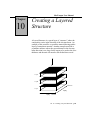
Creating a Layered Structure
89
HOLZ Interactions & Sub-slicing
95
MacTempas User Manual
MacTempas User Manual
Chapter
I
Installing the
Hardware Protection Key
Activating the
Hardware Key and
Personalizing the
Program
Installation
The application MacTempas and its associated files are all compacted in the file MacTempas.sea which is a self-extracting
archive. After double-clicking on the application on the disk,
select a location on your hard disk for placement of the folder
"MacTempas Folder" which will be created automatically as
part of the extraction procedure. There are two versions of
MacTempas supplied on your disk, MacTempasPPC and
MacTempas68K for the PowerPC and 680XX Macintoshes
respectively. You should run the appropriate version for your
machine.
MacTempas uses a hardware copy protection key which must
be installed on your computer. If you already have installed a
key for use with CrystalKit, you do not need a second key to run
MacTempas and you can proceed to the next paragraph describing how to activate the key for running MacTempas. Before
installing the hardware key, drag the file "TRSecurity" found
inside the folder “MacTempas Folder:Put In System Folder:Put
in Extension Folder” to a closed System Folder. If you are running System 7 or later, the file will be automatically placed in
the extension folder within the System Folder. Make sure you
install the init TRSecurity before installing the hardware protection key. Shut down the computer. With the computer turned
off, unplug the keyboard from the back of the computer and
plug the hardware key into the freed up port in the back of the
computer. Connect the keyboard cable to the other end of the
hardware protection key, making sure that all connections are
good. Restart the computer.
Before MacTempas can be run on a new system, you must run
the program, MacTempasKey. Enter your name and affiliation
as appropriate. This program is not required again unless the
program is moved to another machine. At times when the operating system is changed it may also be necessary to run the
Ch.
Installation - p.1
MacTempas User Manual
installation program once more. If this happens, a message will
come up and say to contact Total Resolution or to run the installation program.
Changing Hardware or Versions
of the MacOS
If you have just changed your computer or installed a new clean
version of the MacOS, you must ensure that the extension
TRSecurity is placed on the new machine/new extension folder.
Without the extension in place, the program will not recognize
the hardware key and MacTempas will run in demonstration
mode.
MathLib is a shared library that is used on PowerMacs. When
MacTempas runs on a PowerMac it uses the math routines that
are contained in the file Mathlib. Unfortunately, the first MathLib provided by Apple was very poorly optimized and thus the
Mathlib provided with MacTempas is intended for your use in
case the version you have on your computer is older than the
one provided with MacTempas. If you are running MacOS 7.5.3
the Mathlib is automatically built into the operating system and
you don’t need the supplied MathLib. The file Mathlib if
present is found in the Extension Folder inside the System
Folder.
Ch.
Installation - p.2
MacTempas User Manual
Chapter
1
Introduction to
Image Simulation
The best High Resolution Transmission Electron Microscopes
(HRTEM) have a resolution approaching 1 Å which sometimes
leads to the erroneous conclusion that using an electron microscope, all atoms in a structure can be resolved. However, it is
not the inter-atomic distances that matter, but rather the projected distances between atoms seen from the direction of the
incident electron. In order to obtain interpretable results, it is
necessary to orient the specimen such that atomic columns are
separated by distances that are of the order of the resolution of
the microscope or larger. This is a condition that very often is
difficult to satisfy and often limits the use of the HRTEM to
studies of crystals only in low order zone-axis orientations.
The HRTEM image is a complex function of the interaction
between the high energy electrons (typically 200keV - 1MeV)
with the electrostatic potential in the specimen and the magnetic
fields of the image forming lenses in the microscope. Although
images obtained from simple mono-atomic crystals often show
white dots separated by spacings that correspond to spacings
between atomic columns, these white dots fall on or between
atomic columns depending on the thickness of the specimen
and the focus setting of the objective lens[1]. Fortunately, in
many cases it is only necessary to see the general pattern of
image intensities to gain the desired knowledge. However, in
general, the image can be best thought of as a complex interference pattern which has the symmetry of the projected atomic
configuration, but otherwise has no one-to-one correspondence
to atomic positions in the specimen. It is because of this lack of
directly interpretable images that the need for image simulation
arose. Image simulation grew out of an attempt to explain why
electron microscope images of complex oxides sometimes
showed black dots in patterns corresponding to the patterns of
Ch. 1 Introduction to Image Simulation - p.3
MacTempas User Manual
heavy metal sites in complex oxides, and yet other images
sometimes showed white dots in the same patterns[2]. This first
application was therefore to characterize the experimental
images, that is to relate the image character (the patterns of light
and dark dots) to known features in the structure.
Most simulations today are carried out for similar reasons, or
even as a means of structure determination. Given a number of
possible models for the structure under investigation, images
are simulated from these models and compared with experimental images obtained on a high-resolution electron microscope.
In this way, some of the postulated models can be ruled out until
only one remains. If all possible models have been examined,
then the remaining model is the correct one for the structure.
For this process to produce a correct result, the investigator
must ensure that all possible models have been examined, and
compared with experimental images over a wide range of crystal thickness and microscope defocus. It is also a good idea to
match simulations and experimental images for more than one
orientation.
The simulation programs can also be used to study the imaging
process itself. By simulating images for imaginary electron
microscopes, we can look for ways in which to improve the performance of present-day instruments, or even find that the performance of an existing electron microscope can be improved
significantly by minor changes in some instrumental parameter.
Alternatively, based on imaging requirements revealed by test
simulations, we can adjust the electron microscope to produce
suitable images of some particular specimen, or even of some
particular feature in a particular specimen.
Ch. 1 Introduction to Image Simulation - p.4
MacTempas User Manual
Describing the
Transmission
Electron Microscope
In order to simulate an electron microscope image, we need
firstly to be able to describe the electron microscope in such a
way that we can model the manner in which it produces the
image. As a first step, we can consider the usual geometrical
optics depiction of the transmission electron microscope
(TEM).
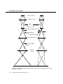
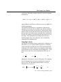
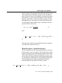
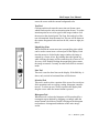
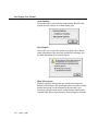
Figure 1 shows such a diagram of a TEM operated in two distinct modes, set up for microscopy (a), and for diffraction (b). In
microscopy mode we see that the TEM consists of an electron
source producing a beam of electrons that are focused by a condenser lens onto the specimen; electrons passing through the
specimen are focused by the objective lens to form an image
called the first intermediate image (I1); this first intermediate
image forms the "object" for the next lens, the intermediate
lens, which produces a magnified image of it called the second
intermediate image (I2); in turn, this second intermediate
image becomes the "object" for the projector lens; the projector
lens forms the greatly-magnified final image on the viewing
screen of the microscope. In microscopy mode, electrons that
emerge from the same point on the specimen exit surface are
brought together at the same point in the final image.
At the focal plane of the objective lens, we see that electrons are
brought together that have left the specimen at different points
but at the same angle. The diffraction pattern that is formed at
the focal plane of the objective lens can be viewed on the viewing screen of the TEM by weakening the intermediate lens to
place the microscope in diffraction mode (b).
Ch. 1 Introduction to Image Simulation - p.5
MacTempas User Manual
Electron Source
Condenser Lens
Object
Objective Lens
Focal Plane of Objective lens
1'st Intermediate
Image
Selected Aperture
Intermediate Lens
2'nd Intermediate
Image
Projecter
Lens
Imaging Mode (a)
Diffraction Mode (b)
Figure 1. Geometrical optics representation of the TEM in imaging mode (a), and
diffraction mode (b)
Ch. 1 Introduction to Image Simulation - p.6
MacTempas User Manual
Simplifying the
Description of the
Microscope
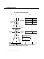
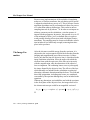
Consideration of the description of the electron microscope in
figure 1 shows that the projector lens and the intermediate lens
(or lenses) merely magnify the original image (I1) formed by
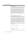
the objective lens. For the purposes of image simulation we can
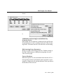
reduce the TEM to three essential components; (1) an electron
beam that passes through (2) a specimen, and then through (3)
an objective lens (fig. 2).
Our next step in describing the electron microscope for image
simulation is to move from the geometrical optics description of
the TEM to a description based on wave optics. In this description of the microscope we examine the amplitude of the electron wavefield on various planes within the TEM, and attempt
to determine how the wavefield at the viewing screen comes to
contain an image of our specimen.
By treating the electrons as waves, and considering our simplified electron microscope (Figure 2), we see that there are three
planes in the TEM at which we need to be able to compute the
(complex) amplitude of the electron wavefield.
(1)The image plane:
Working backwards, we start at our desired information, the
electron wavefield at the image plane; this wavefield is derived
from the wavefield at the focal plane of the objective lens by
applying the effects of the objective aperture and the phase
changes introduced by the objective lens.
(2)The focal plane of the objective lens:
In turn, the electron wavefield at the focal plane of the lens is
derived from the wavefield at the exit surface of the specimen
by a simple Fourier transformation.
(3)The specimen exit surface:
In order to know the exit-surface wavefield, we must know with
which physical property of the specimen the wave interacts, and
describe that physical property of our particular specimen.
Ch. 1 Introduction to Image Simulation - p.7
MacTempas User Manual
The Reduced Electron Microscope
Electron Microscope
Image Calculation
Incident Beam
Specimen
Plane
Specimen
Structure Factors
Ug
Projected Potential
Vp(x,y)
Object Transmission
Function
q(x,y)
Objective Lens
Objective
Lens
Objective
Aperture
Diffraction
Amplitude
Φg
Lens Transfer Function
exp{-iχ(g)}
Lens Aperture Function
Αg
Image
Plane
Image Amplitude
Ψ(x,y)
Fig. 2. The simplified TEM (left) and the calculations required for the image
simulation (right). The three principal planes are marked.
Ch. 1 Introduction to Image Simulation - p.8
MacTempas User Manual
Cowley and Moodie (1957) showed that the interaction of an
electron beam with a specimen could be described by the socalled multislice approximation, in which electrons propagate
through the specimen and scatter from the crystal potential, the
electron scattering is described by the so-called phase-grating
function, a complex function of the potential, and the electron
propagation is computed with a propagation function dependent
on the electron wavelength. Since then there have been numerous formulations of the multislice approximation derived from
the Schrödinger equation.
Simulating TEM
Images
The problem of simulating images thus becomes a problem of
computing the electron wavefields (wavefunction) at three
microscope planes. Currently the best way to produce simulated
images is to divide the overall calculation into three parts:
(1)
Model the specimen structure to find its potential in the
direction of the electron beam.
(2)
Produce the exit-surface wavefield by considering the
interaction of the incident electron wave on the specimen potential.
(3)
Compute the image-plane wavefield by imposing the
effects of the objective lens on the specimen exit surface
wave.
Each of these steps will be covered in the next sections. However, because of space constraints, it is impossible to cover
everything in great depth. For detailed derivation, the reader is
encouraged to read the many excellent texts on the subject.
Ch. 1 Introduction to Image Simulation - p.9
MacTempas User Manual
Ch. 1 Introduction to Image Simulation - p.10
MacTempas User Manual
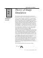
Chapter
2
Modeling the
Specimen
Theory of Image
Simulation
The specimen is a three dimensional objects consisting of a
huge number of atoms. From a modeling point of view, it is necessary to reduce the number of parameters to a more manageable number. For crystalline materials described by a repeat of
perfect unit cells this is easily accomplished. The unit cell in
this case is defined by the lattice parameters A ,B and C where A
and B are in the plane the specimen perpendicular to the electron beam and C is in the main direction of the incoming electrons. A ,B and C are related to the normal lattice vectors a ,b ,
and c depending on the orientation of the specimen. The specimen is thus reduced to M number of unit cells, where M*C is
equal to the thickness of the sample, giving in the end a 2D
image which covers the area given by A and B .
In the case of a defect structure which no longer can be modeled
as a small repeating structure, it is necessary to limit the extent
of the calculation by defining a supercell which contains the
defect. The resulting image obtained from the calculation will
contain artifacts which arise from limiting the structure at arbitrary boundaries and care must be taken to ensure that the image
gives a faithful representation of the area of interest.
The entire electrostatic potential of the specimen is now defined
by one unit cell with axes a ,b , and c , angles alpha, beta and
gamma, and N atoms with coordinates x,y,z. For simplicity, we
use the nomenclature of the crystallographic unit cell even
though we are referring to the transformed unit cell (A ,B ,C ) as
described above.
The electrostatic potential in the crystal can be written
φ (r) = ∫ d 3r'
ρ(r' )
r − r'
1
Ch. 2 Theory of Image Simulation - p.11
MacTempas User Manual
where ρ(r ), the charge density is:
ρ (r) =
∑ ρi (r − ri )
2
all
atoms i
with the sum extending over all atoms i at positions r i, each giving rise to a charge density
ρ i ( r ) = Z i eδ ( r ) − e ψ i ( r )
2
3
where Zi : atomic number, e: electronic charge, ψ (r) : the
quantum mechanical many electron wavefunction for the atom.
The potential φ(r ) is described by its Fourier transform Φ(u)
through the relationship
ϕ (r) = ∫ Φ(u)e −2πiu⋅r du = ∑ Φ(H)e −2πiH⋅r
H
4
since because of the periodicity of the unit cell, Φ(u ) is nonzero only when u = H = ha *+kb *+lc * , H being a reciprocal lattice vector.
The potential Φ(H ) is given as a sum over all atoms in the unit
cell
Φ(H) =
∑ fiel (H)e2πiu⋅r
i
all
atoms i
=
e
4π 2ε 0
∑
all
atoms i
Zi − fi x ( H 2) 2πiu⋅ri
e
H2
5
where the electron scattering factors fiel and the x-ray scattering
factors fix have been calculated from relativistic electron wavefunctions and parameterized. They can be found in various
tables which are used by image simulation programs[3].
Taking into account any deviation from full occupancy at a particular site and the thermal vibration of the atom, the Fourier
coefficients of the crystal potential from one unit cell is calcuCh. 2 Theory of Image Simulation - p.12
MacTempas User Manual
lated as:
Φ(H) =
∑ fiel (H)Occ(ri )exp[− Bi H2 ]e2πiH⋅r
i
6
unit cell
atoms i
B: Debye Waller factor; Occ(r i) : The occupancy at position r i
Simulating the
Interaction
Between the Electrons and the
Specimen
The interaction between an electron of energy E and the crystal
potential φ(r ) is given by the Schrödinger equation
[−
h2
2
2 ∇ − eφ (r)]Ψ(r) = EΨ(r)
8π m
7
where m is the relativistic electron mass and h is Planck’s constant.
Before entering the specimen, the electron is treated as a plane
wave with incident wavevector k 0, k0 =2π/λ, so that the incident electron wave is written
Ψ0 (r) = exp{i(ωt − 2πk 0 ⋅ r)}
8
It is useful to define the quantity V(r ) which will loosely be
referred to as the potential as:
8π 2 me
φ (r)
V (r) =
h2
9
The Schrödinger equation above cannot be solved directly without making various approximations. Depending on how the
problem is formulated, one can derive the most common soluCh. 2 Theory of Image Simulation - p.13
MacTempas User Manual
tions to the electron wavefield at a position T within the specimen.
The Weak Phase Object Approximation
In the Phase Object Approximation (POA)[4], the phase of the
electron wavefunction after traversing a specimen of thickness
T is given as
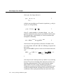
Ψ( x, y, z = T ) ≈ Ψ( x, y, z = 0) exp[ −iσVp ( x, y)T ]
10
with
eE  2
σ = 2πmeλ 1 +
h
mc 

11
where V(x,y) is the average potential per unit length. The specimen is considered thin enough so that electrons only scatter
once and are subject only to an average projected potential. In
the weak phase object approximation, the exponent is considered much less than one, so that the electron wavefunction
emerging from the specimen is:
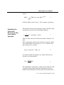
ψ ( x, y, z = T ) ≈ ψ ( x, y, z = 0)(1 − iσVp ( x, y)T )
12
The WPOA only applies to very thin specimens of the order of a
few tenths of Å, depending on the atomic number of the atoms
in the structure[5]. The FT of the wavefunction gives the amplitude and phase of scattered electrons and in the WPOA one has:
Ψ(u) = δ (u) − iσVp (u)T
13
where u is a spatial frequency.
Again, for periodic crystals, Vp(u ) are non-zero only for frequencies u =H where H is a reciprocal lattice vector in the crystal.
We will now use V to mean Vp. Thus for single electron scatterCh. 2 Theory of Image Simulation - p.14
MacTempas User Manual
ing and when the Fourier coefficients V(H ) are real (true for all
centro-symmetric zone axis), the WPOA illustrates clearly that:
i) Upon scattering, the electron undergoes a -90° phase shift.
ii) The amplitude of a scattered electron is proportional to the
Fourier coefficient of the crystal potential.
The Bloch Wave Approximation
In the BWA the electron wavefunction of an electron with
wavevector k is written as a linear combination of Bloch waves
b(k,r) with coefficients ε[6]. Each Bloch wave is itself
expanded into a linear combinations of plane waves which
reflect the periodicity of the crystal potential.
ψ (r) = ∑ ε ( j ) b ( j ) (k, r) = ∑ ε ( j ) ∑ cg( j ) exp[−2πi(k (0j ) + g) ⋅ r] 14
j
j
g
The formulation above gives rise to a set of linear equations
expressed as
( j)
( j)
[k02 − (k ( j ) + H)2 ]cH
+ ∑ V (H' )cH
− H' = 0
15
H'
which needs to be solved. Detailed derivation of the Bloch
wave approximation can be found elsewhere.
Characteristics of the Bloch wave formulation are:
- Requires explicit specification of which reflections g are
included in the calculation.
- Easy to include reflections outside the zero order Laue zone.
- Very good for perfect crystals, not suited for calculating
images from defects.
- The solution is valid for a particular thickness of the specimen.
- Allows rapid calculation of convergent beam electron diffraction patterns.
- Includes dynamical scattering.
Ch. 2 Theory of Image Simulation - p.15
MacTempas User Manual
The Multislice Approximation
The multislice formulation[7,8] is by far, the most commonly
used method of calculating the electron wavefield emerging
from the specimen. Although it does not as easily include scattering outside the zero order Laue zone as the BWA, the multislice formulation is more versatile for use with structures
containing any kind of defects, either they be point-defects,
stacking faults, interfacial structures, etc. The multislice solution gives the approximate solution to the electron wavefunction
at a depth z+dz in the crystal from the wavefunction at z. In the
multislice approximation one has:
z + dz
ψ ( x, y, z + dz ) ≈ exp[−iσdz∇ 2x , y ] ⋅ exp[−iσ ∫ V ( x, y, z' )dz' ]ψ ( x, y, z )
z
16
Thus starting with the wavefunction at z=0, one can iteratively
calculate the wavefunction at a thickness n*dz, by applying the
multislice solution slice by slice, taking the output of one calculation as the input for the next. Equation 16 is solved in a two
step process.
The potential due to the atoms in a slice dz is projected onto the
plane t=z, giving rise to a scattered wavefield
z + dz
ψ 1 ( x, y, z + dz ) = exp[ −iσ ∫ V ( x, y, z' )dz' ]ψ ( x, y, z ) ≡ q( x, y)ψ ( x, y, z )
z
17
The function q(x,y) is referred to as the phasegrating.
Subsequently, the wavefield is propagated in vacuum to the
plane t=z+dz, according to
ψ ( x, y, z + dz ) = exp[ −iσdz∇ 2x , y ] ⋅ ψ 1 ( x, y, z )
18
The last equation represents a convolution in real space and is
Ch. 2 Theory of Image Simulation - p.16
MacTempas User Manual
solved more efficiently in Fourier space[9], where the equation
transforms to
Ψ(H, z + dz ) = exp[−iπλdzH 2 ] ⋅ Ψ1 (H, z ) ≡ p(H, dz ) ⋅ Ψ1 (H, z ) 19
where Ψ(H,z) are the Fourier coefficients of ψ(x,y,z). p(H,dz) is
called the propagator.
The multislice formulation is a repeated use of the last two
equations and will give the wavefield at any arbitrary thickness
T of the specimen. If the slice-thickness is chosen as the repeat
distance of the crystal in the direction of the electron beam, only
the zero order Laue reflections are included in the calculation as
the unit cell content is projected along the direction of the electron beam. Three dimensional information which involves
including higher order Laue reflections can be included by
reducing the slice thickness[10].
Sampling Criteria
Any numeric calculation must be performed for a limited set of
data points (x,y) or reciprocal spatial frequencies u. Working
with periodically repeated structures; if the lateral dimensions
of the unit cell is a and b, which we for simplicity make orthogonal so that the axes are associated with an orthogonal x,y coordinate system, then for a given sampling interval dx=dy, we
have
N=
a
;
dx
M=
b
dy
20
defining the calculation to a grid of N*M points. The sampling
interval automatically restricts the calculation in reciprocal
space as well. The maximum reciprocal lattice vector for
orthogonal axes is given as
2
H 2max = hmax a * + kmax b * =
2
 N
 M
+
 2a 
 2b 
2
21
Ch. 2 Theory of Image Simulation - p.17
MacTempas User Manual
Because most implementations of the multislice formulation
makes use of Fourier transforms, the calculation grid N and M
is adjusted so that both are powers of 2. This is because Fourier
transform algorithms can be performed much faster for powers
of 2 rather than arbitrary dimensions. This results in uneven
sampling intervals dx,dy when a ≠ b. In order to not impose an
arbitrary symmetry on the calculation, a circular aperture is
imposed on the propagator. In practice, this aperture is set to 1/2
of the minimum of (hmax, kmax) as defined above in order to
avoid possible aliasing effects associated with digital Fourier
transforms. The sampling must be chosen such that the calculation includes all (or sufficiently enough) scattering that takes
place in the specimen.
The Image Formation
After the electron wavefield emerge from the specimen, it is
subjected to the varies magnetic field of the lenses that form the
imaging and magnification part of the microscope. Of these
lenses, only the first lens, the objective lens, is considered in the
image formation calculation. Since the angle with which the
electron forms with the optic axis of the lens varies inversely
with the magnification, only the aberrations of the objective
lens are important. The remaining lenses serve to just magnify
the image formed by the objective lens. The effects of the lens
which normally are included in the calculation are spherical
aberration, chromatic aberration and lens defocus. Two-fold and
three-fold astigmatism, including axial coma, are considered
correctable by the operator although they can be included in the
equations.
Without any aberrations, no instabilities and with the specimen
in the focal plane of the objective lens, the image observed in
the electron microscope would be am magnified version of
I ( x, y) = ψ ( x, y, z = exitplane of specimen) = ψ e ( x, y)ψ e∗ ( x, y)
2
22
Ch. 2 Theory of Image Simulation - p.18
MacTempas User Manual
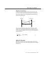
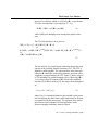
Objective Lens Defocus
Consider an electron traveling from the plane defined by the
exit surface of the specimen to the plane given as the plane of
focus for the objective lens. This distance is referred to as the
objective lens defocus ∆f.
Object plane
Exit plane
∆f/cosα
α
α = Hλ
∆f
The electron traveling along the optic axis will have a path
length of ∆f while an electron that has been scattered an angle
α=Hλ, will travel a distance ∆f /cosα. This can be expressed as
a phase difference
(
)
2π ∆f
− ∆f ≈ πλ∆fH 2
cos
α
λ
23
Spherical Aberration
Electrons crossing the optic axis with an angle a at the focal
plane of the objective lens should form parallel paths emerging
from the lens.
Ch. 2 Theory of Image Simulation - p.19
MacTempas User Manual
α
δ(α)
f
However, the spherical aberration of the lens causes a phase
shift relative to the path of the unscattered electron (α=0) which
is written as[11]:
2π λ ∗ 1 4 Cxα 4 = 1 2 πCs λ3 H 4
24
If there were no other effects to consider, the image would be
obtained as follows:
Calculate the wavefield emerging from the specimen
according to one of the approximations.
Fourier transform the wavefield which gives the amplitude and phase of scattered electrons.
Add the phase shift introduced by the lens defocus and
the spherical aberration to the Fourier coefficients.
Inverse Fourier transform to find the modified wavefunction.
Calculate the image as the modulus square of the wavefield.
However, there are two more effects that are usually considered. Variations in electron energy and direction.
ChromaticAberration/TemporalIncoherence
Electrons do not all have exactly the same energy for various
reasons. They emerge from the filament with a spread in energy
and the electron microscope accelerating voltage varies over the
Ch. 2 Theory of Image Simulation - p.20
MacTempas User Manual
time of exposure. The chromatic aberration in the objective lens
will cause electrons of different energies to focus at different
planes. Effectively this can be thought if as rather than having a
given defocus f0, one has a spread in defocus values centered
around f0. The value f0 is what is normally referred to as ∆f as
indicating defocus. The images associated with different defocus values add to make the final image. Assuming a Gaussian
spread in defocus of the form
( f − f0 ) 2
D( f − f0 ) ∝ exp[−
]
∆2
25
gives:
I=
∫ Ψ( f
2
− f0 ) D( f − f0 )df ⇒ Ψ(H) → Ψ(H) exp[ − 1 2(πλ∆H 2 ) 2 ]
26
This states that each Fourier term (diffracted beam) is damped
according to the equation above[11].
Beam Divergence / Spatial Incoherence
The electron beam is not an entirely parallel beam of electrons,
but form rather a cone of an angle α. This implies that electrons
instead of forming a point in the diffraction pattern form a disk
with a radius related to the spread in directions. As for a variation in energy, the images formed for different incoming angles
are summed up by integrating over the probability function for
the incoming direction. It turns out that this also leads to
another damping of the diffracted beam[12] so that:
2
I (r) = ∫ ψ (r, α ) D(α )dα ⇒ Ψ(H) → Ψ(H) exp[παλ (Cs H 2 λ2 + ∆f )]2
27
Ch. 2 Theory of Image Simulation - p.21
MacTempas User Manual
The Final Image
Equation 26 and equation 27 are only valid when the intensities
of the scattered beams are much smaller than the intensity of the
central beam. Thus the image results from scattered beams
interfering with the central beam, but not with each other. This
is referred to as linear imaging. Although the formulation is
slightly more complicated in the general case, the expressions
above give sufficient insight into the image formation. Image
simulation programs do however include the more general formulation which include non-linear imaging terms[13]. Each
Fourier component is damped by the spread in energy and
direction and the image is formed by adding this to the recipe in
section 4.2
The Contrast Transfer Function CTF
When reading about HRTEM, it is impossible not to encounter
the expression "Contrast Transfer Function". Loosely speaking,
the CTF of the microscope refers to the degree with which Fourier components of the electron wavefunction (spatial frequencies) are transferred by the microscope and contribute to the
Fourier transform of the image. Although the CTF only holds
for thin specimen and linear imaging, it is often generalized and
wrongly applied to all conditions. However, the CTF does provide insight into the nature of HRTEM images. In order to
derive the expression for the CTF, we start by calculating the
image intensity as given by the Weak Phase Object approximation. In the WPOA:
Ψ( x, y, z = T ) ≈ 1 − iσVp ( x, y)T
28
and
Ψ(H) = δ (H) − iσVp (H)T
29
Applying the phase shift due to the spherical aberration and the
Ch. 2 Theory of Image Simulation - p.22
MacTempas User Manual
objective lens defocus which we will call χ(H), we get that the
FT of the wavefunction is (for simplicity V = Vp):
Φ(H) = δ (H) − iσV (H)eiχ ( H ) A(H)
30
where A(H) is the damping terms arising from partial coherence.
The FT of the intensity is now given as
I (H) = FT (ψ ⋅ ψ ∗ ) =
∑ Ψ(H' )Ψ * (H − H' ) ≈
H'
∑ (δ (H' ) − iσA(H' )V (H' )eiχ (H' ) )(δ (H − H' ) − iσA(H − H' )V (H − H' )eiχ (H − H' ) ) ≈
H'
δ (H) + 2σA(H)V (H)sin χ (H)
31
The last result is very useful and it leads to the frequently used
concept of the Contrast Transfer Function (CTF). The CTF is
defined as A(H)⋅sinχ(H) The equation above states that each
reflection H contributes to the image intensity spectrum with a
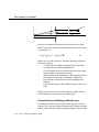
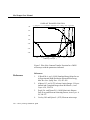
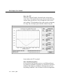
weight that is proportional to the CTF. Figure 3. shows a plot of
a CTF including sinχ and the damping curves. When sinχ (H) =
-1 for a large range of frequencies H, which is the condition
referred to as Scherzer defocus[11], the image can be thought of
as:
I ( x, y) ≈ 1 − 2σU ( x, y)
32
where U(x,y) is a potential related to the original crystal potential, but keeping only the Fourier coefficients related to frequencies transferred by the microscope. The equation above shows
the often used rule of thumb. For thin specimens, under
Scherzer imaging conditions, atoms are black.
Ch. 2 Theory of Image Simulation - p.23
MacTempas User Manual
CONTRAST TRANSFER FUNCTION
V = 200.0 kV Cs = 1.0 mm Def = -560.00 Å Del = 50.00 Å Div = 0.60 mrad
1.00
0.70
0.40
0.10
-0.20
-0.50
-0.80
0.06
0.14
0.22
0.30
-1
0.38
0.46
0.54
Scattering Vector [Å ]
Figure 3. Plot of the Contrast Transfer Function for a 200kV
microscope with the parameters indicated.
References
References
1. O’Keefe M.A. et al. (1989) Simulated Image Maps for use
in Experimental High-Resolution Electron Microscopy,
Mat. Res. Soc. Symp. Proc. 159, 453-458
2. Allpress J.G. et al (1972) n-beam Lattice Images. I. Experimental and Computed Images from W4Nb26O77, Acta
Cryst. A 28, 528-536
3. Doyle P.A. and Turner P.S. (1968) Relativistic HartreeFock X-ray and Electron Scattering Factors, Acta Cryst.. A
24, 390-397
4. Cowley J.M. and Iijima S. (1972) Electron microscope
Ch. 2 Theory of Image Simulation - p.24
MacTempas User Manual
5.
6.
7.
8.
9.
10.
11.
12.
13.
image contrast for thin crystals, Z. Naturforschung 27a,
445-451
Gibson J.M. (1994) Breakdown of the weak-phase object
approximation in amorphous objects and measurement of
high-resolution electron optical parameters, Ultramicroscopy 56, 26-32
Howie A. (1963) Inelastic scattering of electrons by crystals, Proc. Roy. Soc. A271, 268-275
Goodman P, Moodie A.F. (1974) Numerical evaluation of
N-beam wave functions in electron scattering by the multislice method, Acta Cryst. A30, 322-324
Self P.G.et al. (1983) Practical computation of amplitudes
and phases in electron diffraction, Ultramicroscopy 11, 35
Ishizuka K. and Uyeda N. (1977) A new theoretical and
practical approach to the multislice method, Acta Cryst. A
33, 740
Kilaas R. et al. (1987) On the inclusion of upper Laue layers in computational methods in High Resolution Transmission Electron Microscopy, Ultramicroscopy 21, 47-62
Scherzer O (1949) The Theoretical Resolution Limit of
the Electron Microscope, Journal of Applied Physics 20,
20-29
Frank J (1973) The envelope of electron microscope transfer functions for partially coherent illumination, Optik 38,
519-536
O’Keefe M.A. (1979) Resolution-damping functions in
non-linear images, Proc. of EMSA 37, 556-557
Ch. 2 Theory of Image Simulation - p.25
MacTempas User Manual
Ch. 2 Theory of Image Simulation - p.26
MacTempas User Manual
Chapter
3
Introduction to
MacTempas
Since the simulation process can be subdivided into independent calculations involving the structure, the scattering process
and the imaging process, MacTempas allows one to invoke
these independent calculations separately through the “Calculate” menu.
The Three Simulation Steps
Projected Potential
- generates the crystal potential that produces electron scattering from the structural data, unit cell
dimensions, symmetries, and atom positions, occupancies, and
temperature factors.
ExitWavefunctions(s)
- generates the electron wavefield at the
specimen exit surface; it uses projected potential combined with
information about the accelerating voltage of the electron
microscope, and the specimen thickness and tilt. The computation algorithm is the multislice approximation.
Image(s) - generates the image intensity at the microscope
image plane; the effects of the objective lens phase changes and
resolution-limiting aberrations are included via parameters like
defocus, spherical aberration, incident beam convergence,
spread of defocus, and the position and size of the objective
aperture.
wpo - is a separate module that allows the calculation of images
that would be produced in the case of an ideal Scherzer lens and
validity of the weak phase object approximation. The “wpo”
calculation is discussed more in detail elsewhere.
ImagePlaneWavefunctions(s)
-generatestheelectronwavefunction at the imaging plane in the microscope. This is equiva-
Ch. 3 Introduction to MacTempas - p.27
MacTempas User Manual
lent to the application of the Contrast Transfer Function to the
Fourier transform of the electron wavefunction at the exit surface of the specimen followed by an inverse Fourier transform.
The calculation of the image plane wavefunction is used for
comparing with the electron wavefunction found by the use of
electron holography.
Thus “ProjectedPotential
” calculation considers only the specimen structure, “ExitWavefunctions(s)
” calculation treats the
interaction of the specimen with the electron wave, and the
“Image(s) ” calculation simulates how the wave leaving the
specimen interacts with the lens system of the electron microscope. Once a simulation has been made, any additional simulation will usually not require a full re-calculation; any change in
microscope parameters will not affect the results of the “ProjectedPotential ”and“ExitWavefunctions(s)
”calculations,and
only Image(s) will need to be re-run; any change in microscope
voltage or in specimen thickness and tilt will not affect the outputof“ProjectedPotential
”,but“ExitWavefunctions(s)
”and
“Image(s) ” will need to be re-run. Of course, any change in the
specimen structure will require the re-running of all three subprograms.
Generated Files
MacTempas generates and stores various files in the course of a
simulation. The 6 possible data files are:
(1)
<structurename>.at stores all the structure and microscope information needed to run the simulation. This
information is derived from user input and the supplied
data files. In particular, the string “structurename ” is a
unique name for the structure, input by the user when
creating the structure file. This is an editable file of type
‘TEXT’.
(2)
<structurename> .pout is the result of running the
PHSGRT subprogram from the information stored in
<structurename> .at ;itcontainsthespecimenpotential
Ch. 3 Introduction to MacTempas - p.28
MacTempas User Manual
in the direction of the electron beam. This is a BINARY
file of type Real 4. The first 80 bytes consists of record
information and the data starts at byte 80. The first line
of data contains the data for the bottom line of the
“image” since the coordinate system for MacTempas is
at the lower left corner of the image/unit cell. Thus if the
data is imported into a program for viewing, the image
will appear flipped.
(3)
<structurename> .mout is the result of running the
MSLICE subprogram using the data in <structurename> .pout withthosein<structurename> .at ;itcontains the exit-surface wavefunction at one or more
selected specimen thicknesses. This is also a BINARY
file with the same structure as <structurename> .pout,
except for the fact that the data is complex, pairs of
numbers (real and imaginary). The data starts at byte 80
and the file can contain more than one exit wavefunction.
(4)
<structurename> .iout is the result of running the
IMAGE subprogram to apply the effects of the microscope parameters in the <structurename> .at file to the
exit-surface wave; it contains one or more images ready
to be displayed. This again is a BINARY file with data
starting at byte 80 and the file can contain more than one
image. Data is Real 4
(5)
<structurename> .hout is the result of calculating the
image plane electron wavefunction(s) instead of calculating the simulated images. The data is complex, pairs
of numbers (real and imaginary). The data starts at byte
80 and the file can contain more than one image plane
exit wavefunction.
(6)
<structurename> .aout contains the complex amplitudes of several diffracted beams at one-slice increments
in specimen thickness. The beams are specified by the
Ch. 3 Introduction to MacTempas - p.29
MacTempas User Manual
user, and can be plotted as a function of specimen thickness.
In addition, two “print” files are produced (but rarely printed)
just in case additional information about a computation is
required by the user. These files are:
(7)
<structurename >.p_prnt containsinformationabout
the way in which the “ProjectedPotential
” subprogram
processed the <structurename >.at data to produce the
specimen potential.
(8)
<structurename >.m_prnt containsinformationabout
the way in which the “ExitWavefunctions(s)
” subprogram processed the <structurename >.pout data with
the <structurename >.at to produce the exit-surface
wave; that is, it contains information from the multislice
computation.
Ch. 3 Introduction to MacTempas - p.30
MacTempas User Manual
Chapter
4
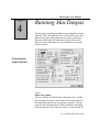
Running MacTempas
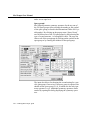
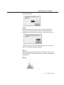
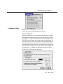
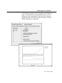
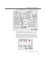
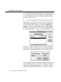
The first step in running a simulation is generating the structure
input file. This is done through New... in the FILE menu. This
generates the input dialog window below which requests the
following information: All fields have default values and in
order to create a valid input file, only valid data for the atoms
must be entered.
Generating an
Input Structure
a, b, c,
alpha, beta, gamma
These are the unit cell dimensions in Ångstrøm units, and the
unit cell angles in degrees. MacTempas will automatically set
the angles depending on the spacegroup, if possible. The program will also automatically set lattice parameters depending
on the spacegroup. Thus if the user chooses a cubic system, b
Ch. 4 Running MacTempas - p.31
MacTempas User Manual
and c are set equal to a
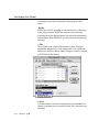
Space group#
MacTempas generates symmetry operators for the any one of
the 230 space groups when selecting the number or the symbol
of the space group (as listed in the International Tables for Crystallography). By clicking on the pop up menu “Space Group”
one can choose one of the 230 spacegroups by first selecting the
type of crystal-structure, i.e. hexagonal or cubic. The user can
choose one of the spacegroups by clicking on the symbol for the
spacegroup or by entering the number for the spacegroup.
The input also allows for choosing the second setting for a specific spacegroup if one exists. If no space group is required, one
should use the space group P1 (1), in which case the only symmetry operator is x,y,z. Additional symmetry operators can be
entered by opening the dialog displaying the symmetry operators.
Ch. 4 Running MacTempas - p.32
MacTempas User Manual
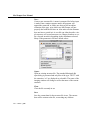
Set Basis
Use this button to bring up the dialog window that enables the
input of the atoms in the basis.
Number of Atoms in the Basis
This value is the number of independent atom positions in the
basis or asymmetric unit of the cell. When operated on by the
symmetry operators, the basis generates all the atom positions
within the cell. This value is never modified by the user since
the program always recalculates this number depending on the
data entered.
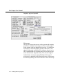
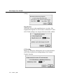
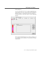
Show (Symmetry Operators)
The symmetry operators are automatically created by specifying the spacegroup. By clicking on this button, a window dis-
Ch. 4 Running MacTempas - p.33
MacTempas User Manual
playing the symmetry operators are shown.
Show (Atoms in Unit Cell)
The atoms in the unit cell are automatically created by the operation of the symmetry operators on the atoms in the basis. The
number of atoms is given and by clicking on the button “Show”,
Ch. 4 Running MacTempas - p.34
MacTempas User Manual
a window displaying the atoms in the unit cell appears.
Number of different atoms
This value is the number of different types of atoms in the specimen structure; difference is due to a different atomic number or
a different Debye-Waller factor. The correct value is calculated
by MacTempas and displayed.
Zone Axis
Specimen orientation in relative real space axes units.
Number of slices per unit cell
For unit cells with large repeat distances in the beam direction,
moderate values of G max may allow the Ewald sphere to
approach the so-called pseudo upper-layer line that the multislice allows at the reciprocal of the chosen slice thickness. In
this case MacTempas will sub-divide the slice into two or more
subslices. How this is done depends upon the potential setting
Ch. 4 Running MacTempas - p.35
MacTempas User Manual
chosen in the Option menu.
Gmax
The maximum value (in reciprocal Ångstrøm units) of any scattering vector to be included in the multislice diffraction calculation. This value imposes an “aperture” on the diffracted beams
included in the dynamic scattering process. It should be large
enough to ensure that all significant beam interactions are
included. The default value is 2.0. MacTempas will compute
phase-grating coefficients out to twice G max in order to avoid
aliasing in the multislice calculations.
Specimen Thickness
The thickness of the specimen foil is entered as a beginning
thickness, an ending thickness and an incremental thickness. All
numbers are in Ångstrøm units. A series of thicknesses represented by the upper and lower bounds and a thickness step; e.g.
100 250 50 will cause MacTempas to store the exit wavefield at
specimen thicknesses of 100Å to 250Å in steps of 50Å (a total
of four thicknesses).
Store Ampl./Phases - Set...
Clicking this button allows a number of diffracted beams to be
selected for plotting of their intensity and phase variation as a
Ch. 4 Running MacTempas - p.36
MacTempas User Manual
function of specimen thickness. The reflections to be tracked
are determined by entering the hkl values for the reflection.
Only 10 reflections can be tracked this way.
Center of the Laue Circle
Specimen tilt is specified by entering the center of the Laue circle in units of the h and k indices of the projected two-dimensional reciprocal-space unit cell. The new indices and their
relationship to the original reciprocal cell is found in the data
file <structurename >.p_prnt
Type of Absorption
Absorption can be included in the program by introducing an
Ch. 4 Running MacTempas - p.37
MacTempas User Manual
imaginary projected potential.
Microscope
The type of electron microscope used to generate the imaging
parameters. Predefined microscopes are shown in the popup
menu together with one undefined microscope. If a predefined
microscope is used, MacTempas provides values for Cs, the
spherical aberration coefficient of the objective lens (in mm.);
DEL, the halfwidth of a Gaussian spread of focus due to chromatic aberration (in Ångstrøm units); TH., the semi-angle of
incident beam convergence (in milliradian). If the type of
microscope is unknown to MacTempas, the above values must
be entered separately (We will see later how a new microscope
Ch. 4 Running MacTempas - p.38
MacTempas User Manual
may be made known to MacTempas).
Voltage
The electron microscope accelerating voltage in kilovolts.
Objective Lens Defocus
The defocus of the objective lens is entered in Ångstrøm units
with a negative value representing underfocus (weakening of
the lens current). As for the SPECIMEN THICKNESS parameter, the input is a range specified by the upper and lower bounds
and an increment.
Cs, Spherical Aberration
The spherical aberration of the objective lens in mm.
Convergence Angle
This is the spread in angle for the cone of incoming electrons
depending on the condenser lens aperture. The angle is given in
mrad.
Spread of Defocus
Ch. 4 Running MacTempas - p.39
MacTempas User Manual
This is the effective spread in defocus which results from the
distribution of energies of the imaging electrons and the chromatic aberration of the objective lens. The unit is Å.
Aperture Radius
The radius of the objective aperture is specified in Å-1
Center of objective Aperture
The center of the objective lens aperture is defined in units of h
and k of the two dimensional reciprocal space unit cell, as for
the Laue circle center.
Center of the Optic Axis
The center of the optic axis of the electron microscope is specified in terms of the h and k indices of the two-dimensional
reciprocal-space unit cell, just as for the Laue circle center and
the aperture center.
Two-fold astigmatism
The two fold astigmatism of the objective lens and the angle
with the x-axis. The magnitude is given in Å.
Three-fold astigmatism
The two fold astigmatism of the objective lens and the angle
with the x-axis. The magnitude is given in Å.
Mechanical Vibration
This simulates the effect of a slight vibration of the microscope.
One finds that often the simulated images show details that are
not present in the experimental data regardless of other imaging
conditions. This may be due to image degradation caused by
microscope vibration or other effects not included and thus one
can introduce a slight mechanical vibration in an attempt to create more realistic simulated images. It is possible to specify an
anisotropic vibration by introducing the amplitude in two perpendicular directions with the diagonal of the ellipse at an angle
with the a axis (as in the unit cell viewed in the zone axis orientation).
Ch. 4 Running MacTempas - p.40
MacTempas User Manual
Chapter
5
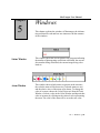
Windows
This chapter explains the windows of Mactempas, the information presented in each and how one interacts with the contents
of the windows.
Status Window
This window shows the current status of the program indicating
the number of phasegrating coefficients calculated, the current
slice number being calculated, the current image being calculated etc.
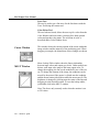
Atom Window
This window shows which atoms are present in the structure,
the color the atom will be drawn in (if colored atoms are set)
and the relative sizes of the atoms to be drawn. To change the
color of an atom, choose the Color Picker tool from the Tools
Window, click on a color in the Color Window and deposit that
color on an atom by clicking on the colored circle representing
the atom. The color of the atom will be set to the new color.
Ch. 5 Windows - p.41
MacTempas User Manual
To change the atomic radius, double-click on the chemical sym-
bol. A dialog window will pop up and a new value for the
atomic radius can be entered (units in Å).
Color Window
Tools Window
This window is used to set the color of a particular atom species, the color of the foreground (the color of lines and text) and
the background color. Colors for use in pseudocoloring is also
picked from the color window. To choose a color, the Color
Picker Tool must have been chosen. To select the foreground
color click on the color with the Option Key held down. Holding down the Option key and the Shift key selects the background color.
The following tools are currently defined:
Eraser
By selecting the eraser tool, the cursor turns into an eraser
which can be used to erase any part of the image screen. Double-clicking the eraser, erases the entire screen. The eraser
Ch. 5 Windows - p.42
MacTempas User Manual
erases the screen with the current background color.
Text Tool
Clicking on this tool turns the cursor into an i-beam cursor
which can be used to select an insertion point for text. To set the
insertion point for text to be typed in the image window click
the mouse at the desired point. The Font, Size and style of the
text is determined from the menu bar. The text will be drawn in
the current foreground color and can be left, canter or right justified.
Magnifying Glass
When selected the cursor turns into a magnifying glass which
can be used to zoom in on a selected part of the display. Each
time the mouse is clicked in the image window, the image is
zoomed by a factor of two. By holding down the Option key
while clicking, the image will be zoomed out by a factor of 1/2
for every click. Double-clicking the magnifying glass returns
the image to normal. Currently no other tools work in zoomed
mode.
Line Tool
This tool is used to draw lines on the display. If the Shift key is
down, only vertical or horizontal lines will be drawn.
Selection Tool
This tool is used to select a portion of the screen for several possible operations such as copying, cutting, histogram computation etc. To select an area, click at a point in the display and
drag the cursor while the mouse button is pressed.
Histogram Tool
When this tool is selected a histogram will be produced for a
rectangular region defined by dragging a rectangle while the
mouse button is held down. Double-clicking on the histogram
tool produces a histogram distribution of the entire image
screen.
Ch. 5 Windows - p.43
MacTempas User Manual
Trace Tool
This tool is used to get a line trace for the line drawn with the
Trace Tool being the current tool.
Color Picker Tool
This tool when selected, allows the user to pick a color from the
Color Window and color atoms, selecting fore-/back-ground
colors and pseudo-color atoms. The selection of color is
described under Color Window above
Cursor Window
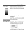
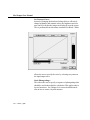
MLUT Window
This window shows the current position of the cursor within the
image window and the intensity of the underlying pixel. When
dragging a rectangle, the dimensions of the rectangle are shown.
Mono Lookup Table window show the linear relationship
between input values and output grey levels. Under normal conditions, each input value maps to the same output value. To
change the mapping, the line can be modified by use of the cursor. To change the contrast of the image, the endpoints can be
moved by the mouse if the mouse is clicked near the endpoint
and the mouse button is held down while the mouse moves. The
brightness is changed by clicking near the center of the line and
dragging it to the desired location. To reset the lookup tables,
just double-click in the MLUT window.
Note: The above only currently works when the monitor is set
to 256 colors.
Ch. 5 Windows - p.44
MacTempas User Manual
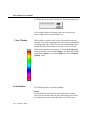
Pseudo Window
Use this window to pseudo color images to enhance certain features in the image. To pseudo-color an image with grey levels,
color is substituted for certain grey levels. To do this, select the
Color Picker Tool, select a color from the Color Window and
deposit the color anywhere in the grey-scale by dragging in the
pseudo-color window. Double-clicking in this window resets
the grey levels.
Source Window
Use this window to define which part of the calculation to display. The choices are:
Projected Potential
- Essentially the output of the PHSGRT
subprogram. There is a one to one correspondence between the
points in the projected potential and those in the image if displayed under equivalent conditions.
Exit Wavefunction
- This is the output of the MSLICE subprogram and shows the distribution of electrons as they emerge
from the bottom of the specimen, or at a predefined depth in the
specimen. By holding down the OPTION key when selecting
the button, one can select to display either the magnitude
squared (default), the complex amplitude or the complex phase
of the electron wavefunction at the exit surface of the specimen.
Ch. 5 Windows - p.45
MacTempas User Manual
Diffraction Pattern
- Select this option to display the diffraction pattern for one of the selected specimen thicknesses. This is
a dynamical diffraction pattern including multiple scattering in
the specimen.
Image - When selected, one of the calculated images becomes
the source of the operations defined by clicking in the Operand
Window. By holding down the OPTION key when selecting the
button, one can select to display either the image intensity
(magnitude squared, default), or if the image plane wavefunction(s) has been calculated, the complex amplitude or the complex phase of the electron wavefunction at the image.
Operand Window
Selecting functions in this window defines the actions to be performed on the source defined by clicking in the Source Window.
Prior to selecting an operation, a source must have been
selected. The operation currently available are:
FFT
Use this to perform a Fourier Transform on the source selected
in the Source Window. Operating on the Projected Potential will
yield the structure factors, operating on the Exit Wavefield will
yield the diffraction pattern and operating on the image will
give the Power spectrum of the image.
#Unit cells
Use this to specify the number of unit cells that should be displayed. The input requires the number of cells in the a-direction
and b-direction. The number of unit cells stay in effect until
Ch. 5 Windows - p.46
MacTempas User Manual
explicitly changed.
Zoom
Use this selection to Zoom the object to either magnify the
object or to reduce the object. A zoom factor greater than 1.
magnifies and a zoom factor less than 1. reduces the object. As
with the number of unit cells to be displayed, the zoom factor
stays in effect until explicitly changed.
Histeq
This operation performs a histogram equalization on the source.
Only a final object of the type “image” is suitable for histogram
equalization.
Histog
Ch. 5 Windows - p.47
MacTempas User Manual
Selecting this operation will produce the histogram of the
source.
Display
Before the result of operating on a selected source is displayed
in the image window, DISPLAY must have been selected.
Choosing the source and operations only selects the functions to
be performed. When DISPLAY gets activated, the functions get
executed.
->File
This will allow for output of the numeric values of images,
amplitudes and phases to a file. Options allow for writing the
data in ascii format or binary format. Images can also be written
as TIFF files in this fashion.
Cancel:
Use this button in case the wrong sequence of commands was
chosen or anything else was entered wrong. This cancels the set
functions.
Ch. 5 Windows - p.48
MacTempas User Manual
Chapter
6
File Menu
Menus
Many of the functions in MacTempas are run from one of the
MacTempas menus, including the multislice calculation. In
addition, most options are set from one of the menus. This is a
list of the currently available menus and a description of their
function.
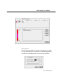
This menu contains the following commands:
Ch. 6 Menus - p.49
MacTempas User Manual
New...
Create a new structure file. A name is prompted for before input
is made. Enter a unique structure name, the program will
append the extension .at. Make sure that you do not add an
extension of the type .at in which case MacTempas will not
properly deal with the file later on. Also make sure the filename
does not have a period in it. A new file can either describe a single structure or a layered structure (see Chapter 8 on how to create a layered structure) depending on the radiobutton selected.
Many of the parameters will have default values.
Open...
Open an existing structure file. The standard Macintosh file
open dialog is presented and only files of the type ‘TEXT” with
the extension “.at” are displayed as selectable. The name of the
imaging window will change to reflect the name of the current
structure.
Close
Close the file currently in use
Save
Save the current data for the structure file in use. The current
data will be written to the file, overwriting any old data.
Ch. 6 Menus - p.50
MacTempas User Manual
Save As...
Save the current structural information. Do not use a name with
an extension if the file being saved is a structure file for later use
by MacTempas.
Save Selection...
Saves the selected portion of the screen into a file. The filetype
(PICT, grayscale Tiff or Palette Tiff) can be selected from the
file Save Dialog.
Save Window...
Saves the content of the image window into a file. The filetype
(PICT, grayscale Tiff or Palette Tiff) can be selected from the
file Save Dialog.
Open PICT File...
Open a PICT file and display it in the MacTempas image window. Only pictures that will fit within the MacTempas image
window can be opened this way.
Page Setup...
Set the options for the page to be printed.
Print...
Print the MacTempas image window. If a Selection is made, the
selection will be printed out. If a histogram window or Trace
Window is the foremost window, that window will be printed.
Quit
Quit MacTempas.
Ch. 6 Menus - p.51
MacTempas User Manual
Edit Menu
Undo
Undo the last operation. This operation does not work in
MacTempas.
Cut
Cut out the selection made by the selection tool. The cut selection can be moved by holding the mousebutton down when the
cursor is within the selected area.
Copy
Copy the selection made by the selection tool. The copied selection can be moved around as described in Cut above.
Paste
Paste a selection onto the image window. The source for the
paste can be an image cut out from another application or
through the cut/copy commands of MacTempas
Clear
Clears the selection made by the selection tool
Select All
Select the entire MacTempas image screen for the next operation.
Ch. 6 Menus - p.52
MacTempas User Manual
Show Clipboard
Shows the clipboard and the content of the clipboard.
Preferences
The maximum size of a calculation and the maximum number
of atoms in MacTempas is by default set to 256*256 and 2500.
These numbers can be changed if the size of the program is
modified accordingly and sufficient memory is present in the
computer. Since running MacTempas with virtual memory
turned on is very slow, all memory requirement should be satisfied by physical Random Access Memory.
Ch. 6 Menus - p.53
MacTempas User Manual
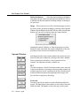
Options Menu
Automatic Erase
Toggles whether the screen is automatically erased before the
image window is being drawn into.
Request Position
Toggles whether you are prompted for the position of the upper
left corner of the image to be displayed.
Automatic Titling
Toggles whether each image will be shown with a descriptive
title below the image
Ch. 6 Menus - p.54
MacTempas User Manual
Atom Overlay
If set, the atom positions will be drawn in as circles on top of
images. The circles are scaled to the atomic radius and the color
is the color set for that atom species. If the Option key is held
down while the image is "drawn", only the circles are drawn (no
image).
Montage...
Brings up a dialog box, allowing the user to select automatic
montage of a series of images, the position of the series of
images and the number of pixels to leave between images.
Intensity Scaling...
Brings up a dialog box, allowing the user to manually set the
intensity values to be mapped to black and white. The values
shown correspond to the last image displayed with automatic
Ch. 6 Menus - p.55
MacTempas User Manual
scaling.
Magnification
Allows the user to set the magnification to a set value. The
magnification depends on a screen with a resolution of 72 dots/
inch. If Auto-scaling is set, images will scale to fit the window.
CTF Scaling...
Brings up a dialog box, allowing the user to set the maximum
scale of the reciprocal axis during plotting of the Contrast
Transfer Function.
Ch. 6 Menus - p.56
MacTempas User Manual
Diffraction Pattern...
Displays a dialog box, allowing the user to select the position of
the diffraction pattern, the camera length and the minimum diffracted intensity that can be displayed. The user can also choose
whether the objective lens aperture should be superimposed on
the diffraction pattern. The indices of the diffracted beams can
be superimposed on the diffraction pattern as well as the corresponding real space distances. Selecting Circular Diffraction
spots instead of Gaussian Diffraction Spots results in solid circles. One can also set a cut-off such that diffracted beams with
g-vectors larger than the cut-off will not be displayed.
Min Lens Intensity...
Displays a dialog box, allowing the user to manually set the
minimum intensity required of a diffracted beam for inclusion
in the formation of the image.
Ch. 6 Menus - p.57
MacTempas User Manual
Atom Shading...
Allows the user to select whether atoms drawn should be displayed in color (circles) or as shaded balls (grey
Slice Method...
Allows the user to select the option to perform a three dimensional calculation of the projected potential by summing over
the third dimension (l) in reciprocal space.
Show Microscopes...
Displays a dialog, showing the user which microscopes are
known to MacTempas. The default parameters associated with a
known microscope can be changed by the user and a new
microscope may be made known to MacTempas. MacTempas
currently only allows a maximum of 10 microscopes to be made
Ch. 6 Menus - p.58
MacTempas User Manual
known
n.
UseFitForElectronScatteringFactors/UseFitForX-Ray
Scattering Factors
MacTempas can use either the 8 parameter fit for the Electron
Scattering Factors or the 9 parameter fit for the X-Ray Scattering factors. The menu item text will reflect the current setting.
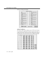
Edit Scattering Factor Parameters...
Brings up a table of the fitting parameters. Double clicking in
the value -field brings up a dialog box prompting for a new
value. See next page.
Treat as Monolayer
When this option is set, the calculation treats the unit cell as a
non-repeating structure such that the entire specimen is represented by a single unit cell with the thickness of the specimen as
the thickness of the unit cell.
Ch. 6 Menus - p.59
MacTempas User Manual
Ch. 6 Menus - p.60
MacTempas User Manual
Commands Menu
Erase
Erases the selection made by the selection tool.
Draw the unit Cell...
Displays a dialog box, from which the user can select to display
the original or transformed unit cell from any direction, including perspective view. The transformed cell corresponds to the
unit cell that MacTempas uses in the multislice calculation. To
view the cell as “seen” by the electrons, the transformed (new)
unit cell should be viewed in the 001 orientation. It should be
noted that the viewing direction is in units of the real space unit
cell axes. One can also view a cross-section of the material in a
given direction. A dialog box allows the user to specify the
field of view in Å for the two directions.
Ch. 6 Menus - p.61
MacTempas User Manual
Draw the CTF
Draws the Contrast Transfer Function for the current microscope values. The original microscope values are taken from the
structure data, but the user is free to change the values associated with the CTF independent of the values used in calculating
the image. By selecting to print with this window being the
front window, the CTF is printed.
Draw Pendelløssung Plots...
In case the user has selected to store a set of diffracted beams
for plotting of amplitudes and phases as a function of specimen
thickness, this brings up a dialog box allowing the user to set
the plotting conditions. One can choose to have the amplitudes
Ch. 6 Menus - p.62
MacTempas User Manual
or the intensities plotted as well as the phases of the diffracted
beams. Each reflection can be plotted by itself, or several
reflections can be superimposed on the same plot. Instead of
plotting the values, the values can also be written to a file for
further manipulation or inspection.
Ch. 6 Menus - p.63
MacTempas User Manual
Set Contrast Curve...
Instead of changing the hardware lookup tables to effectively
change brightness and contrast values, the brightness and contrast can be set before the images are displayed on to the screen.
This is performed from this menu command. Set Black / White
allows the user to specify the curve by selecting two points on
the input/output curve.
Stack Phasegratings...
This allows the user to specify a sequence of phasegratings that
should be used in the multislice calculation. This applies only to
layered structures. See Chapter 9 for a more detailed instruction on how to create a layered structure.
Ch. 6 Menus - p.64
MacTempas User Manual
Slice Unit Cell...
Use this option to subdivide a structure into separate layers for
use in a layered structure calculation. The direction perpendicular to the slices and the number of slices must be specified.
Ch. 6 Menus - p.65
MacTempas User Manual
Parameters Menu
Main Parameters...
This brings up a dialog box showing the current conditions for
the simulation. The values are taken from the input given to the
New... command in the FILE menu. The parameters can be
changed as to bring about a new simulation.
Ch. 6 Menus - p.66
MacTempas User Manual
Atomic Basis...
Brings up the list of all the atoms forming the set of basis atoms
for the current structure. The atomic coordinates etc. can be
edited and atoms can be added to or deleted from the list.
Symmetry Operators...
This brings up the list of symmetry operators either associated
by the space group or entered manually by the user. The symmetry operators can be edited, and new ones may be added to
Ch. 6 Menus - p.67
MacTempas User Manual
the list or existing ones deleted.
Atomic Coordinates...
This shows all the atoms within the unit cell. This list of atoms
are generated by applying the symmetry operators on to the set
of basis atoms above. This list can not be changed, the changes
must take place in the atomic basis or the symmetry operators.
Ch. 6 Menus - p.68
MacTempas User Manual
Calculate Menu
The active commands in this menu depends on the current sta-
tus of the calculation. If the simulation has already been carried
out for the current set of parameters, then no commands will be
active. If a change has been made or the file is a newly created
structure file, the commands showing which subprograms needs
to be run are shown active.
Full Calculation
Use this command if you would like the program to run the
multislice calculation to its end starting from the point required
by the last change made to the simulation parameters.
Projected Potential
Execute this command if you only want to run the PHSGRT
program at this time. After the phasegrating is run, the multislice option is highlighted.
Exit Wavefunctions(s)
Execute this command if you only want to run the MSLICE
program at this time.
Image(s)
Execute this command if you only want to run the IMAGE program at this time.
“Wpo”
This will calculate the weak phase object images for a range of
Ch. 6 Menus - p.69
MacTempas User Manual
resolutions specified by the user. See the introduction and the
later chapter for information on the WPO Approximation and its
use.
Image Plane Wavefunction{s)
This will calculate the complex wavefunction at the image
plane based on only linear terms in the contrast transfer function, i.e. only interference between the central beam and scattered beams.
Statistics Menu
The current operations in this menu are:
Histogram
Displays the histogram distribution of an area selected by the
selection tool, or of the entire image screen if selected through
the Select All command.
Column Average
Shows an average intensity along the horizontal line defined by
the rectangle chosen by the selection tool. The trace being calculated by the program corresponds to the average of the pixels
defined by the width of the rectangle.
This menu determines the appearance of text drawn in the
MacTempas image window. The following text attributes can be
set:
Ch. 6 Menus - p.70
MacTempas User Manual
Text Menu
Font
Size
Style
Left Justified
Center Justified
Right Justified
These are the standard Macintosh menu items for formatting the
text produced by the Text Tool.
Windows Menu
Use this menu to bring a window to the top of the screen in case
it has been completely covered by another window. The use of
the Option Key can make the windows invisible/visible.
Ch. 6 Menus - p.71
MacTempas User Manual
Ch. 6 Menus - p.72
MacTempas User Manual
Chapter
7
Input File Format
The structure file created by New... in the File Menu is a file of
type ‘TEXT’ and can be produced by the editor EDIT. At times
it is desirable to edit the file directly, rather than using MacTempas to create this file. In fact the user may sometimes want to
write a program to generate the data in the structure file. For
that purpose in particular, the format of the structure file <structurename>.at is given below:
Line #Parameter(s)
1
Title
Meaning
Arbitrary description of this
structure
2
SpaceGroupNumber Just as is says, one of the 230
spacegroups, (1-230) including 0.
3
abcabg
The lattice parameters and angles
4
Gmax
The maximum reciprocal lattice
vector in the multislice calculation. The potential is evaluated
out to twice this value, units Å-1.
5
iu iv iw
The direction of the electron
beam in units of the real space
crystal lattice vectors.
6
NSymops Nslices
(I3d)
Number of symmetry operators,
number of slices per unit cell,
and a flag indicating 2d (0) or 3d
(1) potential calculation only if
Nslices is different from 1.
Ch. 7 Input File Format - p.73
MacTempas User Manual
Line #Parameter(s)
Meaning
7
NBasis Ntypes
The number of atoms in the basis,
the number of different types of
atoms. A different type is associated with a different chemical
symbol or a different DebyeWaller factor.
8
it symb x y z
dw occf
The type of atoms (a number
from 1 - NTypes), Chemical symbol, x-,y-,z coordinates in relative
units of the lattice vectors,
Debye-Waller factor and occupancy factor.
9
The same as line 8 for atom number 2.
10
The same as line 8 for atom number 3.
.
8+NBasis
MicName Cs Del Th The name of the microscope, the
spherical aberration (mm), the
spread of defocus (Å) and semiangle of divergence (mrad).
9+NBasis
Voltage
10+NBasis
Lh Lk
Ch. 7 Input File Format - p.74
Accelerating voltage (kVolt).
The center of the Laue circle in
units of the h and k of the transformed reciprocal unit cell. (Real
numbers).
MacTempas User Manual
Line #Parameter(s)
11+NBasis
Thickness
12+NBasis
IPlot
13+NBasis
ih ik il
Defocus
D1,D2,DD
14+NBasis
+NAmp
ApertureRad.
15+NBasis
+NAmp
Ah Ak
16+NBasis
+Namp
Oh Ok
Meaning
The specimen thickness or
T1,T2,DT First thickness, last
thickness, increm. The commas
are required.
Amplitudes to be stored as for
possible plotting, (YES/NO).
The indices of the reflection to be
stored, or if IPlot == NO then :
Objective lens defocus or
First defocus, last defocus, increment. The commas are required.
Radius of the objective lens
Aperture in units of Å-1.
The center of the objective lens
aperture in units of h,k of the
transformed reciprocal unit cell.
The center of the optic axes in the
same units as Ah,Ak.
Ch. 7 Input File Format - p.75
MacTempas User Manual
Line #Parameter(s)
17+NBasis
+Namp
s1,s2,s3
.
17+NBasis
+Namp
+NSymop
istat
18+NBasis
+Namp
+NSymop
Vibration
Meaning
Symmetry operator number 1. An
example is x+1/3,y+5/6,z+1/3.
The commas are required.
The calculation status of this
structure. For a new structure this
should be 1
Halfwidth of mechanical Vibration in A.
Note: If different wordprocessing software is used, Microsoft
Word, Write Now etc., make sure that the text file is saved at the
end as type TEXT.
Ch. 7 Input File Format - p.76
MacTempas User Manual
Chapter
8
Sample Calculation
As an example of a calculation using MacTempas we consider a
BCSCO super-conductor structure. Using the structure determined by Tarascon et al (1988), we show the steps necessary to
input the model structure, examine it, compute the diffraction
pattern and simulated images, and display and print them.
The Structure
As published by Tarascon et al in Phys. Rev. B 37 (1988)
p.9382-9389, the tetragonal structure has the following parameters Space group: I4/mmm
Cell parameters: a=b=3.814Å, c=30.52Å, a=b=g=90
with nine atom positions in the basis:
Atom
Ca
Sr
Bi
Bi
Cu
O(1)
O(2)
O(3)
O(4)
Wyckoff notation
2a
4e
4e
4e
4e
8g
4e
4e
4d
x
0
0
0
0
0
0.5
0
0
0.5
y
0
0
0
0
0
0
0
0
0
z
Occupancy
0
1
0.1097 1
0.3022 0.87
0.2681 0.13
0.4456 1
0.446
1
0.375
1
0.205
1
0.25
0.065
Isotropic thermal parameters for all atoms are fixed at 3.6 Å2.
Ch. 8 Sample Calculation - p.77
MacTempas User Manual
Entering the
Structure
To enter a new structure into MacTempas, we first go to the
FILE menu (Section 3.3), and select New... After entering a
filename in the New File dialog, MacTempas will put up a dialog into which the relevant information must be entered. Note
that many of the input parameters have default values. The only
data that must be entered in ordered to create a valid file is the
atoms in the basis.
Filename
BCSCO
Specify a filename under which to file the input data. It should
be descriptive enough to be easily remembered when you need
to open it later. Make sure you use no extension.
Comment
BCSCO by Tarascon et al
MacTempas has a field for an optional comment or title. The
Ch. 8 Sample Calculation - p.78
MacTempas User Manual
user should enter a comment such as the above, short enough to
fit, yet detailed enough to jog the memory when referred to six
months hence.
Space group #
139
From the structure information, we know that the cell is tetragonal with a space group I4/mmm. From Table 6.2.1 of the International Tables for Crystallography, we find that the space
group number for I4/mmm is 139. Choose the correct spacegroup from the popup menu.
a
3.814
Enter the correct value for the lattice parameter a. In this example MacTempas knows that b is equal to a for the tetragonal
space group #139, and so enters b automatically once a has
been set. Similarly, MacTempas puts in the correct unit cell
angles, since they are defined by the space group (in this particular example). Note that cell parameters are input in Å, not in
nm.
c
The value of the C cell parameter is input in Å.
30.52
Gmax
(default=2)
Gmax is the size of the “multislice aperture” and defines how
far out in reciprocal space the diffraction calculation will
extend. The value of G max is automatically set to 2.0 reciprocal
Ångstrøm units, so that MacTempas will compute all of the
dynamically-diffracted scattered beams out to this value, by
considering all their interactions with phase-grating coefficients out to twice G max (a default of 4.0 reciprocal Ångstrøm
units). Note that these default values (2 for the multislice and 4
for the phase-grating) are normally large enough to ensure that
all significant contributions to the dynamic scattering are
included; however G max is displayed in the MacTempas menu
so that it can be set to a larger value if greater precision is
required with a structure that includes heavy atoms. Note that
MacTempas may be forced to choose a lower value of G max if a
Ch. 8 Sample Calculation - p.79
MacTempas User Manual
large unit cell is used. This occurs because MacTempas has a
limit on the array dimensions used in the multislice calculations. Although this limit can be changed under Preferences ,
the current limit is in effect until the program is restarted. The
array dimensions are required to be powers of two. An upper
limit of 256 by 256 is limited by array dimensions to a parameter-16 multislice calculation (like 256 by 256, or 512 by 128, or
1024 by 64...) so that G max for the diffracted beams is limited to
2n-2a* along one reciprocal-lattice coordinate and to 2m-2b*
along the other, where n+m=16 (hence “parameter-16”). Note
that MacTempas will choose values of n and m to maximize
G max up to the default value of 2.
Zone Axis
0,1,0
The correct response is the set of three integers that defines the
direction of the electron beam with respect to the specimen (or
the specimen orientation with respect to the incident electron
beam direction). In this example we choose to enter 0,1,0 in
order to image the specimen down the b-axis.
Number of slices per unit cell
(default=1)
This value will be computed by MacTempas from the repeat
distance of the structure in the beam direction and the current
value of G max. This number can be changed if desired (as, of
course, can all the parameters entered in response to the
prompts listed in this chapter).
Set Basis
9
Click on the command to bring up the dialog box for entering
the information regarding the number of atoms in the basis. We
enter the nine different atom positions listed for the basis atoms.
For each of the atoms in the basis, MacTempas requires the
chemical symbol, x,y,z coordinates, DW factor and occupancy
factor. From the information given above, we use the following
information for the nine atoms that are given in the structural
basis.
Chemical Symbol
Ca
x,y,z
0,0,0
Ch. 8 Sample Calculation - p.80
MacTempas User Manual
Debye-Waller Factor
3.6
Occupancy
1
The data for the first atom include the chemical symbol for calcium (used by MacTempas to select the correct scattering factor
table), the atom coordinates, the temperature factor (or DebyeWaller factor), and the occupancy factor.
The second atom position is entered in the same way with
responses of Chemical Symbol
Sr
x,y,z
0,0,0.1097
Debye-Waller Factor
3.6
Occupancy
1
The third atom position is similar, except that the occupancy is
set at 0.87 Chemical Symbol:
x,y,z:
B Factor:
Occupancy:
Bi
0,0,0.3022
3.6
0.87
After all nine atom positions have been entered, MacTempas
will need the parameters of the electron microscope for which
to compute the simulation.
Ch. 8 Sample Calculation - p.81
MacTempas User Manual
Microscope
4000EX
If the input microscope name is listed in MacTempas’s microscope file, various operating parameters will be set automatically. If the entered name is unknown to MacTempas, values
will need to be given for each of the operating parameters. In
this example, we use 4000EX, and find that MacTempas sets the
spherical aberration coefficient to 1.0mm, the Gaussian halfwidth of depth of focus to 80Å, and the semi-angle of beam
convergence to 0.5milliradian.
Specimen Thickness
40 80 20
The foil thickness response may be in one of two forms, either a
single value in Ångstrøm units, or a construction combining a
starting and ending thickness with an incremental value. The
construct that we have entered requests MacTempas to store diffraction results for thicknesses starting at 40Å and continuing
through 80Å in steps of 20Å. That is, at specimen thicknesses
of 40Å, 60Å and 80Å.
Store Ampl./Phases
No
As well as storing all the beam amplitudes at specified specimen thicknesses, MacTempas can store a selected few beam
amplitudes at each single-slice increment in thickness, then plot
amplitude (or intensity) and phase as a function of thickness for
any of the stored beams. To store beams for plotting, click on
the command to enter the indices for the reflections that will be
stored. In this starting example we will not be entering any
information here.
Voltage
(400)
The voltage would need to be entered if an unknown microscope type were selected. Since we have selected a 4000ex,
MacTempas will choose a value of 400keV.
Center of the Laue Circle
0,0
The pair of values specified as the Laue circle center are used by
MacTempas to define the direction and amount by which the
specimen is tilted from the exact zone-axis orientation specified
Ch. 8 Sample Calculation - p.82
MacTempas User Manual
above, and, in fact, specify the center of the Laue circle in units
of the h and k coordinates in the diffraction plane. Note that the
values supplied need not be integers, but should not define a tilt
of more than a few degrees. The default values of 0,0 specify
exact zone-axis orientation.
Objective Lens Defocus
-200 -800 -200
So far, we have supplied all the information MacTempas
requires to carry out the dynamical diffraction part of the simulation; now we input the imaging conditions. The first imagingcondition prompt is for the objective lens defocus. We choose to
enter four values of defocus by specifying defocus values from 200Å to -800Å in steps of -200Å. Note that a negative value
denotes an objective lens weakened from the Gaussian condition; that is, underfocus is negative.
Aperture Radius
0.67
The value for the radius of the objective aperture should correspond to the radius in reciprocal Ångstrøm units, as measured
from a diffraction pattern exposed with the aperture superimposed. We will enter 0.67 to represent a typical value.
Center of the Objective Aperture
0,0
In order to simulate dark-field images, MacTempas provides for
an objective aperture displaced from the center of the diffraction pattern. As for the Laue circle center, the aperture center is
defined in units of h and k. We leave the default values of 0,0.
Center of the Optic Axis
0,0
To provide for microscope misalignment, or for conditions of
tilted-beam imaging, the coordinates of the diffraction pattern at
which the optic axis lies can be specified in the same manner as
the center of the aperture. Again, we use default values of 0,0.
Verifying the
Input
After the response to the last data-entry prompt, MacTempas
draws the windows it uses. To re-display the input information
Ch. 8 Sample Calculation - p.83
MacTempas User Manual
click on the "Main Parameters" in the Parameters menu. At
this stage any desired changes can be made by using the mouse
to move the cursor to the desired parameter, and making the
change.
When all the data in the top field are satisfactory, we go to
"Atomic Basis" in the parameters menu to check that all atom
parameters have been entered correctly. At this stage it is also
worthwhile getting MacTempas to display a model of the structure by.going to the Commands menu and clicking on "Draw
the Unit Cell".
Running the Calculation
When we are satisfied that all data are correct, we run the simulation by.clicking on "Full Calculation" in the calculate menu.
Note that MacTempas displays the current status of the calculation in the Status Window. First, MacTempas computes the
phase-grating for the structure (the status window shows the
number of coefficients generated so far), then the dynamical
diffraction for each slice of the specimen (current slice number
is shown in the Status Window), then four images are computed
at each of the three specimen thicknesses that we specified (the
image number is shown in the window).
Displaying the
Results
Once MacTempas has finished the computation, the results (diffraction patterns, images and diffractograms) can be displayed.
(Also beam amplitude and phase plots if any of these has been
stored).
To display the images, we.go to the source window and select
"IMAGE", then "DISPLAY". MacTempas will ask which of
the 12 images is to be displayed, then display the requested
image in the center of the screen. To increase the area of image,
keeping the magnification the same, select "#CELLS" in the
source window, and double the size in the x direction by choosing 2 unit cells in this direction and one in the y direction; then
Ch. 8 Sample Calculation - p.84
MacTempas User Manual
select "DISPLAY".
To get all 12 images onto the display screen simultaneously,
select the options menu and the "Montage" option. Back in the
source window, set "ZOOM" to 0.5 (to reduce the image magnification in order to fit all 12 images on the screen), then "DISPLAY".
Now go back to the montage option and deselect "Montage".
To display the projected potential for comparison with images,
select "PROJ.POT" in the source window, then "DISPLAY".
Notice that the current values of "ZOOM" and "#CELLS"
remain set from the last update.
To display the diffraction patterns at the stored specimen thicknesses, select "DIFFR.PATT" in the source window, then "DISPLAY". To change the size of the patterns, choose "Diffr. Patt".
from the Options Menu and choose a different camera length.
The size of the diffraction spots also depend on the divergence
angle set in the main parameters. It may be necessary to adjust
both the camera length and the divergence angle to get a suitable display of the diffraction pattern.
To display the power spectrum of one of the images, we choose
"IMAGE" from the source window. Respond by answering
which image and then choose "FFT" from the operand window.
Finally click on "DISPLAY" to view the power spectrum. The
options for the power spectrum are the same as those for display
of diffraction patterns. The circle drawn in diffraction patterns
and power spectra corresponds to the objective aperture and can
be turned off from the diffraction option.
Ch. 8 Sample Calculation - p.85
MacTempas User Manual
Ch. 8 Sample Calculation - p.86
MacTempas User Manual
Chapter
9
The Weak Phase
Object Approximation
The Weak Phase Object (WPO) approximation is a useful tool
to find out what kind of information about a specific structure
may be revealed at different levels of resolution.
The WPO approximation has already been described earlier,
and some of that information is repeated here.There are two
important assumptions that are made in the WPO approximation.
Wavefunction
Approximations
The wavefunction of the electron can be written as
Ψ ( x, y ) = 1 – iσtΦ ( x, y )
where Ψ ( x, y ) is the electron wavefunction at a point (x,y) and
Φ ( x, y ) is the projected electrostatic potential at the same point.
Sigma is the interaction parameter between the electron and the
potential of the atoms and t is the specimen thickness. This first
approximation is good for very thin specimens containing light
atoms.
Ideal Scherzer
Lens
An ideal Scherzer lens is a lens that transfers all diffracted
beams with a g-vector that is less or equal to 1/resolution, and
blocks all diffracted beams with a larger g-vector. In addition it
adds a phaseshift of 90 degrees (relative to the central beam) to
all beams passing through the lens. This in addition to the 90
degree phaseshift introduced by the scattering event itself (the
‘i’ in the equation for Ψ ( x, y ) above) causes all scattered
beams that pass through the lens to be 180 degrees out of phase
Ch. 9 The Weak Phase Object Approximation - p.87
MacTempas User Manual
with the central beam.
Under the two assumptions above, the image intensity in the
WPO approximation can be written as
Ψ ( x, y ) = 1 – iσtΦ ( x, y )
such that the image intensity is low in areas of high electrostatic
potential, the location of atoms. Atoms of higher atomic number show up as larger and darker regions in the image. This
type of image will often be similar in appearance to images calculated by a full multislice calculation for equivalent resolution
for a thin specimen for Scherzer defocus.
The WPO approximation is invoked from the menu bar in the
same fashion as the multislice calculation. The input to the
WPO calculation is a starting resolution in Å and an ending
resolution. The steps in resolution can be fixed (user determined) or automatic. When automatic steps are chosen, the
program will calculate the first image corresponding to the
reflections that lie within 1/BeginningResolution and each new
image will be calculated for the next set of reflections corresponding to a higher resolution until the end resolution is
Ch. 9 The Weak Phase Object Approximation - p.88
MacTempas User Manual
reached.
Ch. 9 The Weak Phase Object Approximation - p.89
MacTempas User Manual
Ch. 9 The Weak Phase Object Approximation - p.90
MacTempas User Manual
Chapter
10
Creating a Layered
Structure
A layered Structure is a special type of “structure” where the
composition varies in the direction of the electron beam. An
example of this would be a crystalline material having surface
layers of amorphous material. Another example would be a
crystalline structure where the repeat distance in the electron
beam direction is too large for the repeat to be used as the slicethickness and the unit cell must be sub-divided into several
e-
LayA
LayB
M Points
LayC
B [Å]
A [Å]
N Points
Ch. 10 Creating a Layered Structure - p.91
MacTempas User Manual
slices with different atomic content. As an example we will
work with three layers which we will call LayA,
LayB and LayC. Each of these “layers” are what we would call
a “single” structure. That means they are defined as a unit cell
with lattice parameters and atomic content. The one thing they
have in common is that the lattice parameters A and B with
respect to the electron beam are the same and that we will use
identical sampling in each case, see figure above.
The idea of the layered structure is that the 3 layers can be
arranged in any chosen sequence to make up the total structure.
The steps in creating and calculating the image for a “layered ”
structure are as follows.
1)
Define the 3 layers LayA, LayB and LayC as single
structures with the same unit cell dimensions perpendicular to
the electron beam (A and B).
2)
Calculate the phasegrating for each structure LayA,
LayB and LayC using the same value for Gmax.
3)
Now create a “New ” Structure in MacTempas using the
Ch. 10 Creating a Layered Structure - p.92
MacTempas User Manual
option “Layered Structure
”. You will be asked to fill out infor-
mation regarding the lattice parameters A and B etc. There are
no input for atoms, because a layered structure has no atom
information per se. Even though you are asked to fill out a
specimen thickness, this value has no meaning at this time,
because the content of the structure has not been defined. The
values of A and B come from the structures LayA, LayB and
Ch. 10 Creating a Layered Structure - p.93
MacTempas User Manual
LayC. When you create the layered structure, a default value of
2 Å-1 is supplied and you must change it in the main parameters
if a different value was used in calculating the phase-gratings
for LayA, LayB and LayC.
4)
Once the information in 3) has been filled out, the file is
created and you must define the “structural” or “phasegrating”
content of the layered structure. This is done by going to the
Command Menu and executing the command “Stack Phasegratings ”. If this is a new file, there will be no phasegratings
listed and the command “New ” must be used to define the layers. By invoking “New ”, you get a list of the available phaseg-
rating files (—.pout ). Double Click on LayA.pout and fill in
the value for the slice-thickness that was used in the calculation
of LayA.pout. Continue and do the same for LayB and LayC.
Now the program has information as to which phase-gratings it
can use and the final part is to define the sequence of these phasegratings up to the desired thickness. Use “Stack ” and the
sequence can be defined in different ways. One way is to type
Ch. 10 Creating a Layered Structure - p.94
MacTempas User Manual
in the sequence as
1,1,1,1,1,1,2,2,2,2,2,23,3,3,3,3,1,1,1 where 1 stands for LayA,
2 for LayB and 3 for LayC. One can also use the commands to
define the sequence. At all times the specimen is drawn as a
colored bar at the left. Once this is done, you have defined the
structure.
5)Now check the Main Parameters to see that everything is correct and finally run the calculation. The calculation will begin
with multislice.
Ch. 10 Creating a Layered Structure - p.95
MacTempas User Manual
Ch. 10 Creating a Layered Structure - p.96
MacTempas User Manual
Chapter
11
HOLZ Interactions
& Sub-slicing
With suitable algorithms, it is possible to include in the diffraction calculation the effects of out-of-zone scatterings, or nonzero (or higher-order) Laue zone (HOLZ) interactions. Basically, there are four ways to produce the set of phasegratings (or
projected potentials) that describe the “multisliced” crystal. For
structures with short repeat distances in the beam direction, the
simplest method is to use one slice per unit cell. For structures
with large repeats in the beam direction, several methods may
be used, three of which rely on sub-dividing the slice into “subslices”. Any of the four methods can be used in MacTempas.
Identical slices with only one sub-slice per unit
cell repeat distance
A multislice computation in which every slice is identical contains no information about the variation in structure along the
incident beam direction, and includes scattering interactions
with only the zero-order Laue zone (ZOLZ) layers. For structures with short repeat distances in the beam direction such a
computation is adequate, since the Ewald sphere will not
approach the (relatively distant) high-order zones.
Identical sub-slices with n sub-slices per unit cell
repeat distance
For structures with large repeats in the beam direction, a
method of sub-dividing the slice is required in order to compute
the electron scattering with sufficient accuracy. The simplest,
but most approximate method, is to compute the projected
Ch. 11 HOLZ Interactions & Sub-slicing - p.97
MacTempas User Manual
potential for the full repeat period then use 1/n of the projected
potential to form a phase-grating function that can be applied n
times to complete the slice. This method avoids interaction
with any “pseudo-upper-layer-line” (Goodman and Moodie,
1974), but ignores real HOLZ layers.
Sub-slices based on atom positions
An improvement on sub-dividing the projected potential is to
sub-divide the unit cell atom positions. In this procedure the list
of atom positions within the unit cell is divided into n groups
depending upon the atom position in the incident beam direction. From these sub-sliced groups, different projected potentials are produced to form n different phase-gratings, which are
applied successively to produce the scattering from the full
slice.
Sub-slices based on the three-dimensional potential
A further improvement on sub-dividing the atom positions, is to
sub-divide the three-dimensional potential of the full slice,
since an atom with a position within one sub-slice can have a
potential field that extends into the next sub-slice. Rather than
compute a full three-dimensional potential and then integrate
over appropriate sub-slices (a 128x128x128 potential would
require over two million samples to be stored), it is possible to
derive an analytical expression for the potential within the subslice z0 ± ∂z projected onto the plane at z0 (Self et al., 1983). It
is possible to apply this method routinely to structures with
large repeats in the beam direction, thus generating several different phase-gratings for successive application, and even to
structures (perhaps with defects) that are aperiodic in the beam
direction and require a large number of individual non-repeating phase-gratings (Kilaas et al., 1987).
Ch. 11 HOLZ Interactions & Sub-slicing - p.98
MacTempas User Manual
MacTempas sub-slicing
While ensuring that the calculation remains sufficiently accurate, MacTempas will normally choose the simplest (and quickest) method of specifying how slices are defined for any
particular combination of specimen, zone axis, accelerating
voltage, and maximum g. To this end, the user can choose to
neglect HOLZ interactions if these are judged to be unimportant. If HOLZ interactions are important, then the user should
select the “3D-Potential Calculation” radiobutton in the Options
menu, rather than “2D-Potential Calculation”.
When a two-dimensional calculation is selected, MacTempas
will use one slice per cell if the cell repeat distance in the beam
direction is small. If the repeat distance is too large for one
slice per unit cell, MacTempas will avoid pseudo-upper-layerlines by producing n identical sub-slices.
When a three-dimensional calculation is selected, (3D-Potential
Calculation activated), MacTempas uses a sub-divided threedimensional potential when the repeat distance is large, and
defaults to one slice per cell if the distance is small enough.
Note that the number of sub-slices per unit cell can be forced to
be greater than one by setting it explicitly in the Parameter
menu; this will ensure that any HOLZ interactions are included
even for small repeat distances. Of course, if the repeat distance
is very small, leading to a distant HOLZ in reciprocal space,
both the calculation and the experiment it is modeling will
interact only very weakly with the HOLZ reflections.
Ch. 11 HOLZ Interactions & Sub-slicing - p.99
MacTempas User Manual
Use of the Layered Structure option to produce the scattering
from a structure that is layered or aperiodic in the incident beam
direction is effectively an application of the method of sub-slicing based on atom positions. Thus the user could create a number of sub-slices by assigning selected atoms to different
structure files, then forming a phasegrating for each sub-slice,
and using the Stack Phasegratings command to specify how the
sub-slices are to be used to describe the specimen structure.
This is the suggested method to try first if upper Laue layers are
to be included or 3-dimensional effects are important as it is
much faster than using a complete 3D calculation.
Other methods
Van Dyck has proposed other methods to include the effects of
HOLZ layers, including the second-order multislice with potential eccentricity (Van Dyck, 1980) and the improved phase-grating method (Van Dyck, 1983). Tests of these procedures show
that the extra computation involved in using potential eccentricity may be worthwhile, but that the improved phase-grating
method diverges too easily to be useful.
Goodman P, Moodie AF (1974) Numerical evaluation of Nbeam wave functions in electron scattering by the multislice
method. Acta Cryst. A30, 322-324.
Kilaas R, O’Keefe MA, Krishnan KM (1987) On the inclusion
of upper Laue layers in computational methods in high resolution transmission electron microscopy. Ultramicroscopy 21,
47-62.
Self PG, O’Keefe MA, Buseck PR, Spargo AEC (1983) Practical computation of amplitudes and phases in electron diffraction. Ultramicroscopy 11, 35-52.
Van Dyck D (1980) Fast computational procedures for the sim-
Ch. 11 HOLZ Interactions & Sub-slicing - p.100
MacTempas User Manual
ulation of structure images in complex or disordered crystals: A
new approach. J. Microscopy 119, 141-152.
Van Dyck D (1983) High-speed computation techniques for the
simulation of high resolution electron micrographs. J. Microscopy 132, 31-42.
Ch. 11 HOLZ Interactions & Sub-slicing - p.101