1
1
SYMBOLIC COMPUTATION AND PARALLEL SOFTWARE
Paul S. Wang1
Department of Mathematics and Computer Science
Kent State University, Kent, Ohio 44242-0001
Abstract
Two aspects of parallelism as related to symbolic computing are presented: (1) the
implementation of parallel programs for the factorization of polynomials, and (2) the automatic derivation and generation of parallel codes for finite element analysis. The former
illustrates the use of parallel programming to speed up symbolic manipulation. The latter
shows how symbolic systems can help create parallel software for scientific computation.
Through these two case studies, the promise of parallelism in symbolic computation is
demonstrated.
1. Introduction
Significant development in parallel processing hardware have taken place in recent
years. There are a wide variety of parallel architectures. A number of parallel processors are now available commercially at different price ranges. These parallel systems
include message passing computers, shared-memory multiprocessors, systolic arrays, massive SIMD machines, as well as multiprocessing supercomputers. Together they promise
to further speed up computations, especially through explicit parallel programming. However, the full potential of such systems can not be realized without similar advances in
parallel software.
At Kent we have been interested in symbolic computation and in applying parallelism
to realistic problems. Here, we will examine two such efforts: parallel polynomial factorization, and automatic generation of parallel programs for finite element analysis. By
these two case studies, we hope to show that parallelism can speed up symbolic computations and, on the other hand, symbolic computing techniques can help create parallel
1
Work reported herein has been supported in part by the National Science Foundation under Grant
CCR-8714836 and by the Army Research Office under Grant DAAL03-91-G-0149
2
software. More details can be found in [16] and [17], respectively.
Our presentation focuses on work at Kent. However, the application of parallelism
is a very active research area within the symbolic computation community. The reader
is referred to the proceedings of the International Workshop on Computer Algebra and
Parallelism for more information [6].
2. Parallel Factoring
2.1 Strategy Outline
Consider factoring a univariate polynomial U (x) of degree n > 0 with integer coefficients into irreducible factors over the integers Z. Without loss of generality, we assume
that U (x) is primitive (gcd of coefficients is 1) and squarefree (no repeated factors) [14].
U (x) is NOT assumed monic and applying a monic transformation on U (x) is not advisable. Instead, leading coefficient handling techniques are applied. This speeds up considerably the factoring of non-monic polynomials which occur often in practice, especially
when univariate factoring is used as a sub-algorithm for multivariate factorization.
The polynomial U (x) is first factored modulo a suitably selected small prime p.
U (x) = u1 (x) u2 (x) ... ur (x) mod p
(1)
where ui (x) are distinct irreducible polynomials over Zp . We know that r ≥ t, the number
of irreducible factors of U (x) over Z. If U (x) is irreducible mod p, i.e. r = 1, than it is
irreducible over Z. If r > 1, the factors of U (x) mod p are lifted to factors of U (x) mod pe
for e sufficiently large. The actual factors of U (x) over Z can then be derived from these
lifted factors.
If r > t then there are extraneous factors mod p that do not correspond to factors over
Z. Extraneous factors complicate and slow down the lifting process and the recovery of
actual factors.
It is advisable to use a prime that gives a value of r as close to t as possible. The fastest
sequential implementation uses several primes to reduce r. We suggest to compute (1) for
several primes in parallel and to use the information obtained to reduce the number of
factors for the later stages of the factoring process. Factorization modulo each different
3
prime is also parallelized by using a parallel Berlekamp algorithm.
Once (1) is computed, we go into the parallel EEZ lifting algorithm using multiple
processes to compute the correction coefficients and to update all factors. Early detection
of true factors will be included with correct handling of the leading coefficient. When
processes are available, the polynomial arithmetic operations required in parallel EEZ
lifting can also be parallelized. After lifting, actual factors can be found in parallel by
simultaneous test divisions and grouping of extraneous factors.
A parallel package called PFACTOR has been implemented in C. PFACTOR takes
an arbitrary univariate polynomial with integer coefficients of any size and produces
• A prime p
• A set of irreducible factors ui (x) mod p
• Information on grouping of extraneous factors for lifting
The output is much simpler if U (x) is found to be irreducible.
To illustrate the parallel operations, the parallel extraction of factors through gcd
operations in the parallel Berlekamp algorithm is presented. Timing data obtained on
the Sequent Balance are also presented. But before we can do that, a few words on the
parallel machines used are in order.
2.2 Shared-Memory Multiprocessors
The PFACTOR package has been implemented on the shared-memory multiprocessor
(SMP) Encore Multimax and later ported to the SMP Sequent Balance. Performance
tests and timing experiments have been conducted on both parallel computers. These
SMPs are relatively common and should be familiar to most students of parallel systems.
Therefore, we will describe them only briefly.
The Encore Multimax at Kent consists of 12 National Semiconductor NS32032 processing elements, each a 32-bit processor capable of executing 0.75 MIPS. The main memory
of 32 MB is shared by all processors. The Multimax has architectural features for fast
memory access and for avoiding bus contention. The Sequent Balance is very similar but
offers 26 processors.
4
The Multimax runs under the Umax 4.2 operating system which is compatible with
Berkeley 4.2bsd (and most of 4.3bsd). In addition to all the usual UNIX facilities, Umax
provides multiprocessing, employing all the CPUs available to support concurrent processes by running up to 12 (in our case) of them simultaneously. The processors are shared
by all system and user processes.
The C language is extended with parallel features [18] and augmented by parallel
library routines. Programming primitives for allocating shared memory, synchronization and timing of parallel processes are provided. An interactive debugger dealing with
multiple processes also exists. The Sequent Balance runs under Dynix, a dual-universe
operating system combining Berkeley 4.2bsd and AT&T system V. The Balance operates
under the same principles while providing a somewhat different set of parallel library
functions.
For both SMPs, parallel activities are initiated in a program by creating child processes
that execute independently but simultaneously with the parent process. Each process is
essentially a separately running program. Communication among a group of cooperating
parallel processes is achieved through shared memory. Data stored in shared memory by
one process are accessible by all related processes with the same shared address space
(Fig. 1). A program can generate many child processes. But if they are going to be
executed in parallel, the total number of processes is limited to the total available CPU’s.
2.3 Parallel Factoring Modulo Different Primes
To obtain factors modulo an appropriate prime in preparation for the EEZ lifting
stage, PFACTOR uses several different primes and performs the following three major
parallel steps in sequence. The output of PFACTOR is the shortest list of factors modulo
the largest prime used.
1. Parallel choice of small primes and load balancing
2. Parallel Berlekamp algorithm on each prime simultaneously
3. Parallel reconciliation of factors
PFACTOR keeps a list of small primes from which several are chosen in parallel to
5
A1
6
P1
A2
. . .
Ak−1
6
P2
6
. . .
Pk−1
Ak
6
Pk
?
Shared
Memory
Figure 1: Private and Shared Address Spaces
satisfy two conditions: (i) the prime does not divide the leading coefficient of U (x) and
(ii) U (x) stays squarefree modulo the prime. The parallel Berlekamp algorithm involves
• Parallel formation of the (n × n) matrix Q−I [10].
• Parallel triangularization of Q−I to produce a basis of its null space.
• Parallel extraction of factors with greatest common divisor (gcd) computations.
The dimension of the null space of Q−I is r, the number of irreducible factors mod p.
Because r ≥ t, U (x) is irreducible over Z if r = 1. If this is the case for any prime used,
then all other parallel activities are aborted and the entire algorithm terminates.
After the factors are obtained for several different primes in parallel, the results can
be put through a degree compatibility analysis which can infer irreducibility and deduce
grouping of extraneous factors.
2.4 Parallel Implementation of PFACTOR
PFACTOR consists of eight modules written in the C language with parallel extensions, system and library calls on the SMP used. Two input parameters are important in
controlling the parallel activities of PFACTOR.
• procs: the total number of parallel processes to use.
6
P1
P1
P2
... Pk−1
P1 1 ... P1 a
...
Pk
Pk 1 ... Pk b
Figure 2: Parallel Process Hierarchies
• k: the total number of primes to use.
For example procs = 9, k = 3 means “factor U (x) mod three different primes, all in
parallel with nine processes”. The primes to use can be specified in the input or generated
by PFACTOR. For simultaneous execution of the processes to take place, the parameter
procs is limited by the number of actual processing elements available to the user. If
procs = 1 then sequential processing is forced which is useful for comparative timing and
debugging purposes. The following cases are considered.
1. If procs = k then procs factorizations are performed in parallel each with one process
and a different prime.
2. If procs < k then the first procs factorizations are performed in parallel each with
one process; then k is set to k − procs. In this case k must be an integral multiple
of procs.
3. If procs > k then all k factorizations are carried out in parallel each with one or
more processes (Fig. 2).
Let us consider case 3 further. If k = 1 then all processes are used for the parallel
Berkekamp algorithm with the given prime. If k > 1, the number of processes assigned
to each finite field factorization is made proportional to the amount of work required in
the Berlekamp algorithm which is roughly pi n2 log n + n3 . Thus, the number of processes
psi used to carry out factoring mod pi is set to the maximum of 1 and
7
(n + pi ) procs
round
P
k n + ki=1 pi log n
!
(2)
for all but the largest prime which gets all the remaining processes. For example, distributing 11 processes for the four primes 7, 11, 23, and 37, with n = 8 under this scheme
results in 1, 2, 3, and 5 processes for each prime factoring respectively.
2.5 Finding Factors in Parallel
In the parallel Berlekamp algorithm, we first form Q − I and obtain a basis for its null
space in parallel. This is followed by the parallel extraction of factors by gcd operations.
It is this last operation that we will discuss in some detail.
Coming into this part of the computation are a prime p, the polynomial u(x) =
U (x) mod p of degree n, ps the number of processes to use, the dimension r of the null
space which is the number of factors to be found. If r = 1 all parallel processes will
terminate.
At this stage we have a set of r > 1 basis polynomials vi (x), 1 ≤ i ≤ r, in increasing
degree with v1 = 1 and we are ready to perform the gcd computations
gcd (f (x) , vj (x) − s)
(3)
for f (x) a divisor of u(x), all vj (x), 1 < j ≤ r and all 0 ≤ s < p. Such computations
are performed until the r irreducible factors of u(x) are found. There are two ways to
parallelize computations for (3).
In the dynamic scheduling scheme, each process can take an f (x) and a vj (x) and
perform all the gcd computations for the different s values. In the beginning, one process
takes on f (x) = u(x) and v2 (x) and breaks up u(x) into two factors: a gcd g(x) and a
quotient h(x). The task [g(x), v3 (x)] is put on a shared task queue to be picked up by
a second process while the first process continues with gcd operations on h(x). When a
process is finished with its task, it goes back to pick up another on the task queue. If the
task queue is empty, the process has to wait. The job is done when all r factors are found.
This scheme works pretty well when there are many factors to find. The only draw back
is that not enough parallelism is applied in the beginning. It degrades to a sequential
8
algorithm if u(x) has only two factors.
Alternatively, the computations required by (3) can be computed by employing all ps
processes for the prime p all the time. In this parallel scheme two lists, facs and nfacs, of
factors of u(x) are kept in shared memory. Initially facs contains only u(x) and nfacs is
empty. For each basis polynomial vj , j > 1 the following is done.
One factor, called the current factor, is removed from facs. Each of the ps processes
computes gcd’s of the current factor (initially u(x)) with the current vj (x)−s for a distinct
subset of s values in parallel. The union of the subsets covers all possible s values. Any
factors found are deposited in the shared list nfacs until either the current factor is reduced
to 1 or all ps processes are finished. By the end of this procedure, one or more factors
whose product is equal to the current factor will have been put on nfacs. Now if facs
is not empty then a new current factor is removed from facs and the procedure repeats.
Otherwise, if facs is empty, then the values of facs and nfacs are interchanged and used
with the next vj (x). The entire process is repeated until r factors are found.
To further illustrate this parallel procedure, we set forth the essential parts of the
parallel C program in the following pseudo code. The code is executed in parallel by
each of the ps processes. Every process has a unique integer process ID, 0 ≤ pid < ps.
Variables in all upper case letters are shared.
par_findfacs(u(x),v1(x),v2(x),...,vr(x),r,pid,ps)
NFACS=(u(x));
FACS=();
foreach v in (v1 ... vr)
{
if (all r factors found) then
break out of foreach loop;
interchange(FACS,NFACS);
par_gcd(FACS,NFACS,v,r,pid,ps);
}
return(concatenate(FACS,NFACS));
par_gcd(FACS,NFACS,v,r,p,id,ps)
9
while (FACS not empty)
{
if ( all r factors found ) then return;
cf = remove first factor from FACS;
n = deg(cf);
NDEG = 0;
if (cf linear) then { put cf on NFACS; NDEG = NDEG +1; }
else
{
s = p - pid - 1;
while(s >= 0)
{
if (NDEG == n) break out of while loop;
g = gcd(cf,v - s);
if (g != 1) then
{
put g on NFACS; NDEG = NDEG + deg(g);
if (NDEG == n) break out of while loop;
cf = cf/g;
}
s = s - ps;
}
/* end of inner while */
} /* end of else */
}
The simplified pseudo code does not show the synchronization or mutual exclusion necessary in a working program. The roles of the shared variables FACS and NFACS are clear.
The shared variable NDEG keeps a running total of the degrees of factors inserted onto
NFACS. When NDEG is equal to n, the original degree of cf, then the current factor is
finished and it is time to process a new cf.
2.6 Performance of PFACTOR
To test the performance of PFACTOR, the degree 40 polynomial, f40 (x), in SIGSAM
problem 7 is used [9]. Over Z, f40 (x) has four irreducible factors
10
a1 (x) = 8192 x10 + 20480 x9 + 58368 x8 − 161792 x7 + 198656 x6
+ 199680 x5 − 414848 x4 − 4160 x3 + 171816 x2 − 48556 x + 469
a2 (x) = 8192 x10 + 12288 x9 + 66560 x8 − 22528 x7 − 138240 x6
+ 572928 x5 − 90496 x4 − 356032 x3 + 113032 x2 + 23420 x − 8179
a3 (x) = 4096 x10 + 8192 x9 + 1600 x8 − 20608 x7 + 20032 x6
+ 87360 x5 − 105904 x4 + 18544 x3 + 11888 x2 − 3416 x + 1
a4 (x) = 4096 x10 + 8192 x9 − 3008 x8 − 30848 x7 + 21056 x6
+ 146496 x5 − 221360 x4 + 1232 x3 + 144464 x2 − 78488 x + 11993
Table 1 and 2 show the timing results obtained by factoring polynomials of increasing
degrees using different number of primes and processes on the Sequent Balance with 26
processors. (See [18] for Encore timings.)
In Table 1 f20 = a1 (x) a2 (x), f30 = a1 (x) a2 (x) a3 (x). Factoring a1 (x) mod 11
and 13 yields its irreducibility over Z through degree reconciliation. The primes used are
automatically selected by PFACTOR.
TABLE 1: PFACTOR Timing Results
Polynomial Degree No. factors
a1 (x)
f20 (x)
Primes
No. processes
Time (secs.)
10
1
11,13
1
0.733075
10
1
11,13
2
0.537024
10
1
11,13
4
0.532023
10
1
11,13
8
0.616446
20
4 (11)
11,13,17
1
4.123983
20
4 (11)
11,13,17
3
1.957521
20
4 (11)
11,13,17
4
1.447737
20
4 (11)
11,13,17
5
1.323721
20
4 (11)
11,13,17
7
1.236876
20
4 (11)
11,13,17
8
1.183241
20
4 (11)
11,13,17
9
1.273457
The effect of additional processes on the speed depends on the size of n, the prime, and
the way a particular problem yields factors in the gcd process. Because of the overhead
11
of creating and managing parallel processes together with associated shared memory the
speed gain for small problems is negligible or even negative. Table 2 shows that as the
problem gets larger, the effect of additional parallel processes becomes considerable. But,
because of the large grain size and the available parallelism in the factoring problem, as
programmed, a point is soon reached beyond which adding more processes will not help
much or even slow down the solution. In the timing tables the number of factors and the
prime returned by PFACTOR are indicated.
TABLE 2: PFACTOR Timing Results
Polynomial Degree No. factors
f30 (x)
Primes
No. processes
Time (secs.)
30
4 (19)
11,13,17,19
2
8.667184
30
4 (19)
11,13,17,19
4
4.907284
30
4 (19)
11,13,17,19
6
4.076474
30
4 (19)
11,13,17,19
8
3.475885
30
4 (19)
11,13,17,19
9
3.304873
30
4 (19)
11,13,17,19
12
2.837887
30
4 (19)
11,13,17,19
16
2.421841
30
4 (19)
11,13,17,19
20
2.359714
30
4 (19)
11,13,17,19
23
2.242413
40
5 (19)
11,19,29,83
4
24.733351
40
5 (19)
11,19,29,83
8
12.573750
40
5 (19)
11,19,29,83
10
9.283978
40
5 (19)
11,19,29,83
15
6.081470
40
5 (19)
11,19,29,83
16
6.152311
PFACTOR can also be used to simply supply a parallel Berlekamp algorithm on a single
prime by simply specifying the prime and the number of processes to use. TABLE 3
shows the timings of factoring f40 mod (83).
12
TABLE 3: Parallel Berlekamp Performance
Polynomial Degree No. factors Prime
f40 (x)
No. processes
Time (secs.)
40
13
83
1
23.161704
40
13
83
2
13.516763
40
13
83
3
10.212376
40
13
83
4
7.960593
40
13
83
5
6.577850
40
13
83
10
4.474641
40
13
83
15
3.831011
40
13
83
20
3.795774
40
13
83
21
3.877265
3. Symbolic Generation of Parallel Programs
Having examined how parallel programs can help speed up polynomial factoring, one
of the central computations in symbolic and algebraic computation, we now turn our
attention to the topic of how symbolic systems can help create parallel software through
automatic program generation.
3.1 Background
Computer scientists and engineers at Kent State and Akron Universities have been
involved in an interdisciplinary investigation of advanced computing techniques for engineering applications. A major focus of this collaboration has been finite element analysis
(FEA) which, of course, has many applications.
Symbolic computation is employed to derive formulas used in FEA. The derived formulas can be automatically fabricated into numeric codes which are readily combined
with existing FEA packages such as NFAP [3] and NASTRAN [5]. The objectives are to
reduce routine but tedious formula manipulations, to avoid mistakes in manual computations, and to provide flexibility in situations where new formulations, new materials or
new solution procedures are required. The techniques developed however is general and
can be applied to generate programs in many other areas.
13
An area of great promise is the development of techniques to exploit parallelism in
engineering computations. For the well-defined area of FEA, our approach to employ parallelism is to automatically generate the desired parallel programs based on the problem
formulation. This approach can make parallel software much easier to create for many
specific areas in science and engineering. By building the expertise needed to take advantage of parallelism into a software system, it is hoped that the powers of advanced
parallel computers can be brought to a larger number of engineers and scientists.
Extending our efforts in the automatic generation of sequential FEA codes, a system
can be built to map key FEA computations onto a given parallel architecture and generate
efficient parallel routines for these computations. For our investigations, we have experimented with the Warp systolic array computer as well as the SMPs. The availability of
these computers at Kent made our research much easier.
Because many FEA problems in practice require super-computing speeds, we have
also extended our investigations to generating Cray Fortran codes to take advantage of
the vectorization and parallel processing capabilities of the multiprocessor Cray computers. A free-standing code generator, GENCRAY, has been constructed to take derived
formulas and render them into correct CFT77 codes. The GENCRAY system defines an
input language that also allows the specification of parallel executions.
3.2 Generating Parallel FEA Codes
We have access to different types of parallel computers: the Warp [1] systolic array
computer, the SMPs, and the 8-processor CRAY-YMP. We are investigating parallel FEA
on all these machines. Here we will focus the work on the Warp.
The Warp
The Warp machine is a high-performance systolic array computer designed for computationintensive applications such as those involving substantial matrix computations. A systolic
array architecture is characterized by a regular array of processing elements that have a
nearest neighbor interconnection pattern. The Warp we used consists of a SUN-3 host
connected, through an interface cluster processor, to a linear systolic array of 10 identical cells, each of which is a programmable processor capable of performing 10 million
14
floating-point-operations per second (10 MFLOPS). A 10-cell Warp, therefore, has a peak
performance of 100 MFLOPS. The Sun-3 host runs under UNIX and provides a parallel
operating and debugging environment [2] for the Warp array. A Pascal-like high-level language called W2 [7] is used to program Warp. The language is supported by an optimizing
compiler.
All cells can execute the same program (homogeneous) or different programs (heterogeneous). Aside from the per-cell instructions, a cell program also specifies the inter-cell
communication through the use of the send and receive primitives. A send statement
outputs a 32-bit word to the next cell while a receive statement inputs a 32-bit word from
the previous cell. There are two I/O channels X and Y between each pair of neighboring
cells. The first cell can use receive to obtain parameters passed by the host program and
the last cell can use send to return results to the host program. An overview of the Warp
system is shown in Fig. 3.
Host
6
?
Interface
Unit
-
Cell
1
Cell
2
......
......
......
Cell
n−1
Cell
n
Figure 3: Overview of Warp System
Finite Element Analysis on the Warp
We can map key portions of finite element computations onto the Warp array. The
generated cellprograms run under the control of a C program that is also generated. At
run time, the C program initiates Warp executions when requested by a generated f77
code module that is invoked by a large existing finite element analysis package, NFAP.
15
We have ported NFAP to run under the SUN-3. The generated f77 module prepares input
data that are passed to the cellprograms through the C program. Results computed by the
cellprograms are passed back through the C program as well. Fig. 4 shows the relations
between these program modules.
NFAP
6
?
Generated f77
module
6
?
Generated C
module
- Cellprogram 1 -
. . .
- Cellprogram n
Figure 4: Program Interfaces
Finite element analysis is computation-intensive. It involves repetitions of the same
algorithm for all the elements covering a given problem domain. Major computational
tasks include discretization of the problem domain into many finite elements, computing the strain-displacement matrix and the stiffness matrix for each element, assembling
the global stiffness matrix and its subsequent solution. We have selected the straindisplacement and the stiffness computations as our first targets for parallelization on the
Warp.
Given the Warp architecture, we examined various parallel algorithms to compute the
strain-displacement and the stiffness matrices. The required W2 code is generated together with the necessary f77 module and the C module to control cellprogram execution.
A software system P-FINGER, a parallel extension of FINGER, is constructed to derive
the necessary sequential and parallel code modules. An extension to GENTRAN [7],
GENW2 [13], is also made to fabricate W2 codes. Generated cell programs may involve
declarations, I/O statements, flow control, data distribution, subroutines, functions and
16
macros.
Timing Experiments on the Warp
Two timing tables are presented here. Each row entry represents a complete stiffness
computation involving Two-D Four-node elements in the isoparametric formulation. Each
run involves a number of Warp invocations. For our timing experiment, each invocation
processes only 100 elements. Thus, for example, the 2000-element entry involves 20 Warp
invocations. The total time for all Warp invocations is accumulated using a timing mechanism written in C. The sequential timing is obtained by using one Warp cell to run the
equivalent sequential code. Times given are in seconds and do not include times used on
the Sun-3 host.
TABLE 4: Homogeneous Parallel Processing
Timings for actual Warp Executions
Two Dimensional Four-Node Elements
No. of Sequential
Elements
SIMD
Speed Up Efficiency
WARP Monitor
100
2.36
0.60
3.9
39
300
7.10
1.56
4.6
46
500
11.64
2.72
4.3
43
1000
22.64
4.67
4.8
48
2000
45.16
8.86
5.0
50
3000
68.20
14.14
4.8
48
4000
89.17
18.79
4.8
48
5000
116.12
24.52
4.8
48
TABLE 5:Heterogeneous Parallel Processing
Timings for actual Warp Executions
17
Two Dimensional Four-Node Elements
No. of Sequential
Elements
MIMD
Speed Up Efficiency
WARP Monitor
100
2.36
0.64
3.7
37
300
7.10
1.42
5.0
50
500
11.64
2.10
5.5
55
1000
22.64
4.14
5.4
54
2000
45.16
7.38
6.1
61
3000
68.20
11.60
5.8
58
4000
89.17
14.82
6.0
60
5000
116.12
18.38
6.3
63
3.3 A CFT77 Code Generator for the CRAY
Many compute-intensive scientific and engineering problems require supercomputing
speeds. Thus, it is also important to generate programs that runs on a Cray. We have implemented a new code translator/generator called GENCRAY. The output of GENCRAY
is f77 or Cray Fortran-77 (CFT77) code with vectorization and parallel features. CFT77
is a superset of f77 and is the standard Fortran available on Cray supercomputers.
One of the outstanding features of GENCRAY is to allow parallel specifications in the
input and to generate codes that take advantage of the vectorization and parallel features
on multi-processor Cray systems
The C language is used to implement GENCRAY so that it is readily portable to
any computer systems with a standard C compiler. GENCRAY also defines its own input
language so it can interface with formulas and procedures derived by any symbolic system.
3.4 Generating Vectorizable/Parallel Code in CFT77
The Cray CFT77 compiler is a vectorizing compiler. Much computing power can
be derived from vectorization if the loops in the program are written so that they are
vectorizable. Properties such as data dependencies across iterations, breaks in flow control
(exiting the loop prematurely), and so on, can prevent vectorization. Also the CFT77
18
compiler only attempts to vectorize the innermost loop. It is up to the programmer
to analyze the structure of nested loops and to arrange them so that vectorizing the
innermost loop reaps the most benefit.
To make it easier to produce vectorizable code, GENCRAY provides several high-level
vectorization macros for matrix/vector computations:
• mmult - matrix multiplication
• madd - matrix addition
• msub - matrix subtraction.
In the generated code these macros expand inline to do loops that are vectorizable and
optimal for the natural algorithms used. For example, consider the matrix multiplication
macro:
(mmult a b c 100 400 250)
The code generated for this is:
c *** BEGIN GENERATED CODE ***
integer m0
integer m1
integer m2
c ** BEGIN MATRIX MACRO EXPANSION **
do 1001 m0=1,250
do 1002 m1=1,100
c(m1,m0)=a(m1,1)*b(1,m0)
1002
continue
1001 continue
c
do 1003 m0=1,250
do 1004 m1=1,100
do 1005 m2=2,400
c(m1,m0)=c(m1,m0)+(a(m1,m2)*b(m2,m0))
19
1005
1004
continue
continue
1003 continue
c ** END MATRIX MACRO EXPANSION **
c *** END GENERATED CODE ***
The Cray YMP is a family of shared memory parallel computers. Each processor is
basically a Cray processor. For instance, the Cray YMP at the Ohio Supercomputer
Center is an eight-processor system. It is, therefore, important for GENCRAY to also
provide easy-to-use facilities for generating CFT77 programs that take advantage of the
parallelism offered by multiple processors. Thus, in addition to vectorization macros,
GENCRAY provides several high-level parallel constructs for generating parallel programs
that use the multiple processors.
The idea is to provide access to the Cray multitasking library primitives through a set
of very high level statements that are much easier to use for specifying a number of useful
parallel executions. GENCRAY can translate these high-level statement into multitasked
programs for the Cray. The following capabilities are provided:
1. Multitasking: The pexec macro is used to specify the parallel execution of several
tasks. Logically, when control flow reaches pexec, it splits into several independently running threads each to execute one of the parallel tasks. When all of its
parallel tasks are done then pexec is finished. The pexec macro is suitable for
actions of relatively coarse granularity due to the overhead involved in setting up
and synchronizing the tasks. The macro can be used, for example, to call several
subroutines in parallel. GENCRAY does not check for data dependencies in the
tasks which can invalidate the parallel execution. It is the user’s responsibility to
ensure that no such dependencies exist.
2. Pipelining: The macro pipe specifies a coarse-grain pipeline program that organizes
multiple processors into an assembly line. It provides a simple way to specify the
stages of a computation and the data transfer from one stage to the next. For
example, pipe can be used to specify a pipeline of forward FFT, element-wise
20
multiplication, and then inverse FFT. GENCRAY translates the pipe macro and
generates CFT77 codes for each stage of the pipeline with correct data transfer and
synchronization.
3. parallel do loop: Also supported by GENCRAY is the macro doall. The different
statements in a doall are executed independently and simultaneously. The doall
can be used to specify parallel tasks with a finer granularity than that in the pexec
construct. Doall is best used in nested loops so that the innermost loop can be
vectorized while the outer loop iterations are executed in parallel.
4. On-going and Future Work
Parallel polynomial factorization work on the SMPs is continuing at Kent. Strategy
details are being ironed out and parallel C codes are being written for the lifting and the
true-factors phases. A package called BigNum [11] developed in France is used to supply
the extended precision integer arithmetic required in lifting. Parallel polynomial arithmetic routines are also implemented to allow additional speed up in the right situations.
The new codes will be combined with PFACTOR to serve as the base of future work on
parallel multivariate factorization.
Another focus of our on-going research is to parallelize many key FEA computations
on SMPs and automatically generate such parallel programs. We will not only extend our
work on the Warp to the SMP but also look into the parallel solution of the global matrix.
Element-by-element (EBE) iterative schemes using preconditioned conjugate gradient are
promising on SMP’s. The EBE scheme works well with many cases in linear analysis. On
the other hand, it encounters difficulties in other cases especially for nonlinear analysis.
When it is applicable, the EBE scheme can be a very efficient parallel method.
A software package is also being developed to generate parallel FEA codes for the
SMPs [12]. This package will feature a way for the engineering user to specify basic computations using familiar notations. These basic numeric computations can be mapped
onto a particular parallel architecture and executed in parallel. The load balancing and
synchronization details will be handled by the derived code.
5. Conclusions
21
Parallel computers are here to stay and to provide important speed up for many different kinds of computations. As more people apply parallel programs to solve problems,
the gap between the highly developed parallel architectures and the primitive parallel
programming tools and operating environments becomes increasingly clear. We are at
a point in parallel software development that sequential programming was before FORTRAN. Much work lay ahead in the parallel software area.
1. High-level parallel programming languages and tools to make parallel software much
easer to write and test.
2. Program portability to make a parallel program usable across a set of parallel computers.
3. Parallel language features to better accommodate the needs of parallel algorithm
designers.
4. Closer collaboration among language, operating system, and architecture specialists
to develop machine features to support the development and execution of parallel
software.
5. Closer collaboration between computer professionals and applications people to target parallel features for practical use.
6. Symbolic computation can benefit from parallelism and can help produce parallel
software.
It is hoped that the mutually beneficial relations between symbolic computation and
parallel software continue to develop and strengthen, and will play an important part in
the overall advancement of parallel computation.
References
[1] Annaratone, M., Arnould, E., Gross, T., Kung, H. T., Lam, M. S., Menzilcioglu, O.,
and Webb, J. A., “The Warp Machine: Architecture, Implementation and Performance,” IEEE Trans. on Computers, Vol. C-36, No. 12, Dec. 1987, pp. 1523-1538.
22
[2] Berlekamp, E. R., “Factoring Polynomials over Finite Fields,” Bell System Tech. J.,
V. 46, 1967, pp. 1853-1859.
[3] Bruegge, B., “Warp Programming Environment : User Manual,” Department of Computer Science, Carnegie Mellon University, Pittsburgh, PA, 1984.
[4] Chang, T. Y., “NFAP- A Nonlinear Finite Element Program, Vol. 2 - Technical
Report,” College of Engineering, University of Akron, OH, 1980.
[5] “COSMIC NASTRAN USER’S Manual,” Computer Services, University of Georgia,
Athens, GA, 1985.
[6] Dora D. J. and Fitch, J. ed., Computer Algebra and Parallelism, Academic Press, San
Diego, CA 92101.
[7] Gates, B. L., “A Numerical Code Generation Facility for REDUCE,” Proceedings,
ACM SYMSAC’86, Waterloo, Ontario, July 1986, pp. 94-99.
[8] Gross, T. and Lam, M., “A Brief Description of W2”, Department of Computer
Science, Carnegie Mellon University, Pittsburgh, PA, 1985.
[9] Johnson, S. C. and Graham, R. L., “SIGSAM Problem #7”, ACM SIGSAM Bulletin,
Feb. 1974, page 4.
[10] Knuth, D. E., The Art of Computer Programming, Vol. 2:Seminumerical Algorithms,
2nd ed., Addison-Wesley, Reading, Mass., USA, 1980.
[11] Serpette, B., Vuillemin, J., and Hervé, J.C., “BigNum: A Portable and Efficient
Package for Arbitrary-Precision Arithmetic,” Digital Equipment Corp., Paris Research Laboratory, 85, Av. Victor Hugo. 92563 Rueil-Malmaison Cedex, France.
[12] Sharma, N. and Wang, P. S., “Generating Finite Element Programs for Shared
Memory Multiprocessors,” Symbolic Computations and Their Impact on Mechanics,
PVP-Vo. 205, American Society of Mechanical Engineers, pp. 63-79, Nov. 1990.
[13] Tan, T. and Wang, P. S., “Automatic Generation of Parallel Code for the Warp
Computer,” Proceedings, 1st International Workshop on Computer Algebra and
23
Parallelism, June 1988, Grenoble, France, Computer Algebra and Parallelism, pp.
91-117, Academic Press, Oct. 1989.
[14] Wang, P. S. and Trager, B. M., “New Algorithms for Polynomial Square-free Decomposition over the Integers,” SIAM J. Computing, Vol. 8, No. 3, Aug. 1979, pp.
300-305.
[15] Wang, P. S., “Parallel p-adic Constructions in the Univariate Polynomial Factoring
Algorithm,” Proceedings, MACSYMA Users’ Conference 1979, Cambridge, MA,
MIT pp. 310-318.
[16] Wang, P. S., “Parallel Univariate Polynomial Factorization on Shared-Memory Multiprocessors,” Proceedings of the ISSAC’90, Addison-Wesley (ISBN 0-201-54892-5),
Aug. 1990, pp. 145-151.
[17] Wang, P. S., “Applying Advanced Computing Techniques in Finite Element Analysis,” Symbolic Computations and Their Impact on Mechanics, PVP-Vo. 205, American Society of Mechanical Engineers, pp. 189-203, Nov. 1990.
[18] Wang, P. S. and Weber, K., “Guide to Parallel Programming on the Encore Multimax,” Technical Report (CS-8901-03), Dept. Math and C.S., Kent State University,
Kent, OH, 44242 USA.