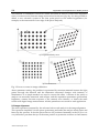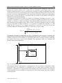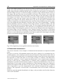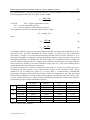
1
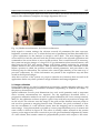
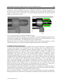
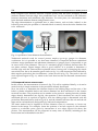
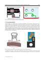
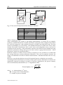
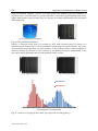
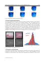
28
Digital Image Processing for Quality Control on
Injection Molding Products
Marco Sasso, Massimo Natalini and Dario Amodio
Università Politecnica delle Marche
Italy
1. Introduction
The need to increase quality of products, forces manufacturers to increase the level of
control on finished and semi-finished parts, both qualitatively and quantitatively.
The adoption of optical systems based on digital image processing is an effective
instrument, not only for increasing repeatability and reliability of controls, but also for
obtaining a large number of information that help the easily management of production
processes.
Furthermore, the use of this technology may reduce considerably the total amount of time
needed for quality control, increasing at the same time the number of inspected
components; when image acquisition and post-processing are feasible in real time, the
whole production can be controlled.
In this chapter we describe some quality control experiences carried out by means of a cheap
but versatile optical system, designed and realized for non contact inspection of injection
moulded parts.
First, system architecture (both hardware and software) will be showed, describing
components characteristics and software procedures that will be used in all the following
applications, such as calibration, image alignment and parameter setting.
Then, some case studies of dimensional control will be presented. The aim of this
application is to identify and measure the main dimensional features of the components,
such as overall size, edges length, hole diameters, and so on. Of particular interests, is the
use of digital images for evaluation of complex shapes and dimension, where the distances
to be measured are function of a combination of several geometric entities, making the use
of standard instrument (as callipers) not possible. At the same time, methods used for image
processing will be presented. Moreover, a description of system performances, related to
quality product requirements will be presented.
Second application examines the possibility to identify and quantify the entity of burrs. The
case of a cylindrical batcher for soap, in witch its effective cross-sectional area have to be
measured will be showed, together with a case study in witch burrs presence could bring to
incorrect assembly or functionality of the component. Threshold and image subtraction
techniques, used in this application will be illustrated together with the big number of
information useful to manage production process.
Third, it will be presented a possible solution to the problem of identifying general shape
defects caused by lacks of filling or anomalous shrinkage. Two different approaches will be
www.intechopen.com
556
Applications and Experiences of Quality Control
used, the former that quantifies the general matching of whole images and the latter that
inspects smaller areas of interest.
Finally, an example of colour intensity determination of plastic parts for aesthetic goods will
be presented. This application has the aim to solve the problem of pieces which could
appear too dark or too light with respect to a reference one, and also to identify defects like
undesired striation or black point in the pieces, depending on mixing condition of virgin
polymer and masterbatch pigment. Use of pixel intensity and histograms have been adopted
in the development of these procedures.
2. System description
In this section, the hardware and software architecture of the system will be described.
The hardware is composed by a camera, a telecentric zoom lens, two lights, a support for
manual handling of pieces, and a PC.
The camera is a monochromatic camera with a CCD sensor (model AVT Stingray F201B ®).
The sensor size is 1/1.8”, and its resolution is 1624 x 1234 pixel, with a pixel dimension of 4,4
μm, a colour depth of 8 bit (256 grey levels) and a maximum frame rate of 14 fps at full
resolution. The choice of a CCD sensor increases image quality, reducing noise in the
acquisition phase and the high resolution (about 2 MPixel) leads to an acceptable spatial
resolution in all the fields of view here adopted.
The optics of the system is constituted by a telecentric zoom lens (model Navitar 12X
telecentric zoom.®); the adopted lens is telecentric because it permits to eliminate the
perspective error, which is a very useful property if one desires to carry out accurate
measurements. The zoom system permits to have different field of view (FOV), so the FOV
can vary from a minimum of 4,1 mm to a maximum of 49,7 mm. The zoom is moved by a
stepper driving, and the software can communicate and move it automatically to the desired
position. The utility of this function will be clear later, when the start-up procedure is
explained.
The depth of focus varies with the FOV, ranging from 1,3 mm to 38,8 mm; the mentioned
camera and lens features bring to a maximum resolution of the system of 0,006 mm (FOV 4,1
mm) and a minimum resolution of 0,033 mm (FOV 49,7 mm).
To lights the scene, a back light and a front light were adopted. Both have red light, to
minimize external noise and to reduce chromatic aberration. Moreover they have a coaxial
illumination, that illumines surface perpendicularly and increases contrast in the image
highlighting edge and shapes and improving the general quality of the image. In figure 1.a
the complete system is showed. All the components are managed by a PC, that use a specific
software developed in LabView®.
Its architecture is reported in figure 1.b. It has a user interface, that guides step by step the
operator through the procedures for the different controls. So, the operator is called only to
choose the application to use, then to load pieces in the work area and to shot photos. Every
time he shots, image is acquired and processed (and stored if necessary), so the result is
given almost immediately. If the operator needs to control a production batch, it is also
possible to acquire several images consecutively and then post-process all of them exporting
global results in an excel file.
All this operations are possible thank to the background software, that answer to the
operator input. In fact, when the operator select the kind of control, the software load all the
parameters necessary to the analysis. For each application, the software load all parameters
www.intechopen.com
557
Digital Image Processing for Quality Control on Injection Molding Products
for camera, zoom and lights (that have been stored earlier), and all the information about the
analysis, like calibration, templates for image alignment and so on.
USER INTERFACE
BACKGROUND
SOFTWARE
DATA
STORAGE
PARAMETER
SETTINGS
IMAGE
ACQUISITION
IMAGE
PROCESSING
a)
b)
Fig. 1. a) Hardware architecture; b) Software architecture
With regard to camera settings, the software controls all parameters like time exposure,
brightness, contrast and so on, so when the best mix of parameters had been determined for
a given application, for the analysis is enough to call it back. The same happens for the
zoom control; in fact the software loads the position stored for the selected application and
commands to the zoom driver to move in that position. This is useful because, if necessary,
the system can acquire images of a large FOV to get information about certain features, and
then narrows the FOV and acquire images with higher spatial resolution for capturing
smaller details in the observed object. Each position utilised has been calibrated sooner.
When a position is called, the software restores related parameters, and pass them to the
following step for elaboration. The software also control light intensity, in the same way of
previous components. So, all the information are passed to the acquisition step and then
stored in the acquired images.
After this overview of the system, it’s proper to describe two functions that are used in all
applications before any other operation: image calibration and image alignment.
2.1 Image calibration
Using digital images, two kind of calibration are necessary: spatial calibration (always ) and
illumination and acquisition parameters calibration (depending on material and shape of
the pieces to be analysed).
Spatial calibration convert pixel dimensions into real world quantities and is important
when accurate measurements are required. For the application described below, a
perspective calibration method was used for spatial calibration (NI Vision concept manual,
2005). So, the calibration software requires a grid of dots with known positions in image and
in real world. The software uses the image of the grid and the distance between points in
real world to generate a mapping function that “translates” the pixel coordinates of dots
into the coordinates of a real reference frame; then the mapping can be extended to the
entire image. Using this method is possible to correct perpendicularity error of camera and
scene which is showed in figure 2a. This effect is actually rather reduced in the present
system, as the support has been conceived to provide good mechanical alignment by means
of a stiff column, that sustains camera in perpendicular position with respect to the scene.
www.intechopen.com
558
Applications and Experiences of Quality Control
This method of calibration is however useful and must be used to correct also alignment
error (or rotation error) between image axis and real world axis (fig. 2b). It is also possible to
define a new reference system in the best point/pixel for the studied application (for
example, at the intersection of two edge of the piece analysed).
a) Perpendicularity error
b) Rotation error
Fig. 2. Errors to correct in image calibration
About parameter setting, the problem is represented by transient materials because the light
passes through the material and the dimension measured changes with intensity of
illumination. So a simple method was used to correct this effect. A master of the pieces to
analyse was manually measured with calliper, and the acquisition parameters (particularly
brightness, contrast ant time exposure of the camera) were selected to obtain the same
results with digital image measurement. All this parameters are stored for each application.
2.2 Image alignment
The other operation computed by the software before each analysis is the image alignment.
This operation simplifies a lot the pieces positioning and make the analysis much easier and
faster for the operator. In fact the pieces have to be positioned manually in the FOV so it is
very difficult to put them always in the same position to permit the software to find features
www.intechopen.com
Digital Image Processing for Quality Control on Injection Molding Products
559
for measurement. In order to align every image with the master image that was used to
develop the specific analysis tool, it could be even possible to put a given piece in any
position within the field of view, and let then the software to rotate and translate the image
to match the reference or master image thus to detect features and dimensions. However, for
the sake of accuracy and repeatability, the positioning is aided by centring pin and support
that permit to place the objects in positions that are similar to the master one used for
calibration and parameters setting.
The alignment procedure is based on pattern (or template) matching and uses a crosscorrelation algorithm. So, first is necessary to define a template (fig. 4b) that the software
consider as a feature to find in the image. From this template, the software extracts pixels
that characterize the template shape, then it looks for the pixel extracted in the new image,
using an algorithm of cross-correlation; so is possible to consider the template as a sub
image T(x,y) of size K x L in a bigger image f(x,y) of size M x N (see fig. 4), and the
correlation between T and f at the pixel (i,j) is given by (J. C. Russ, 1994):
C ( i, j ) =
∑∑ T( x , y ) ⋅ f ( x + i, y + j)
∑∑ f 2 ( x + i, y + j) ⋅ ∑∑ T 2 ( x , y )
x
x
y
y
x
(1)
y
Correlation procedure is illustrated by fig.3. Correlation is the process of moving the
template T(x,y) around the image area and computing the value C in that area. This involves
multiply each pixel of the template by the image pixel that it overlaps and then summing
the results over all the pixels of the template. The maximum value of C indicates the
position where T best matches f.
M
(0;0)
K
N
L
(i;j)
T(x;y)
f(x;y)
Fig. 3. Correlation process
This method requires a big number of multiplications, but is possible to implement a faster
procedure: first, the correlation is computed only on some pixels extracted from the
template, to determines a rough position of the template; then, the correlation over all pixels
of the template can be executed in a limited area of the entire image, allowing to reduce
processing time.
www.intechopen.com
560
Applications and Experiences of Quality Control
In fig. 4 the method applied to the first case of study is showed. Fig. 4.a reports the master
image, from which the template (fig. 4b) has been extracted. It’s clear, that only a part of the
master image has been extracted and this part is considered as the feature to be searched in
the entire image. In fig. 4.c is showed an image of a piece to align with the master, in fact, in
this image, the piece has been moved behind and rotated. The software, first search the
template and determines his rotation angle, rotates the image of the same entity to align the
new image to the master. Then it finds the new position of the template and determines the
translation vector from the master, moves the image of the fixed quantity and the new
image is now aligned to the master. Black areas in fig. 4.d, are the results of translation and
rotation of image; they are black because these areas have been added by the process, and a
part of the image has been deleted to keep the same size of the original image. A double
pattern matching is necessary, because of the image reference system is located on the left
top of the image and not in the template centre. So, first pattern matching determines the
rotation angle and the translation vector that have to be applied but uses only the first to
rotate the image. Performing this operation in fact, the new image has the same alignment of
the master image, but the translation vector changes because the rotation is performed
respect to the left up corner of the image. Second pattern matching determines yet the angle
(that now is zero) and the new translation vector that is used to move the image to the same
position of the master. Image can be now processed.
a)
b)
c)
d)
Fig. 4. The alignment process applied to the first case of study
3. Dimensional measurement
This section describes some examples of dimensional measurement on injection moulded
parts.
In fig.5.a it is shown a 3D simplified model of the part to analyse. It is constituted by two
coaxial cylinders, with a ribbing on the left side; the material is Polyamide 66 (Zytel 101). In
fig. 5.b, all the features that have to be measured in quality control process are represented.
It’s important to notice that there are two kind of feature to measure. The dimensions
denoted by numbers 1, 3 and 4 require the identification of two simple feature (edges) of
the part, so this will be a “simple feature” to measure, and a comparison with standard
instrument is possible. Instead, feature number 2, requires the identification of an axis, by
identification of two edges, and the identification of third element (edge of the ribbing) to
measure the distance from the latter to the previous axis. So, three features are required
and is impossible to get this measurement with standard instruments like gauges or
callipers. This represent a second kind of measurement, that will be called “composed
feature”.
Both cases pass through the identification of edges, so the procedure used for their detection
will be now described.
www.intechopen.com
561
Digital Image Processing for Quality Control on Injection Molding Products
a)
b)
Fig. 5. a) the piece to analyse, b) requested features
More techniques are based on use of pixel mask that runs through the image, computing
the sum of products of coefficients of pixel mask with the gray level contained in the region
encompassed by the mask. The response of the mask at any point of the image is (Gonzales
& Woods, 1992):
R = w1 z1 + w2 z2 + ..... + w9 z9 = ∑ wi zi
9
(2)
i= 1
where: wi = coefficient of the pixel mask;
zi = gray intensity level of the pixel overlapped.
Using different kind of mask, different features can be detected. All of them, are detected
when:
R >T
(3)
where T is a nonnegative threshold. Fig. 6 shows different masks for detection of different
features.
-1
-1
-1
-1
8
-1
-1
-1
-1
a)Point
-1
2
-1
-1
2
-1
-1
2
-1
b)Horizontal
edge
-1
-1
-1
2
2
2
-1
-1
-1
c)Vertical edge
-1
-1
2
-1
2
-1
2
-1
-1
d)+45° edge
2
-1
-1
-1
2
-1
-1
-1
2
e)-45° edge
Fig. 6. Different pixel mask for different features
In this application, an easier method, based on pixel value analysis along a pixel line, has
been used. It is a simplification of derivative operators method (Gonzales & Woods, 1992)
that uses gradient operators and analyses gradient vector to determine module and
direction of the vector.
www.intechopen.com
562
Applications and Experiences of Quality Control
Usually, an edge is defined as a quick change in pixel intensity values, that represents
boundaries of an object in the FOV. It can be defined by four parameters:
1. Edge strength: defines the minimum difference in the greyscale values between the
edge and the background;
2. Edge length: defines the maximum distance in which the edge strength has to be
verified;
3. Edge polarity: defines if the greyscale intensity across the edge is rising (increase) or
falling (decrease);
4. Edge position: define x and y location of an edge in the image.
In picture 7.a is represented a part of an edge (black rectangle); first, the software requires
the input of a user-defined rectangle (green in fig 7.a) that it fixes as the ROI in which to
look for the edge. Then the software divides the rectangle using lines parallel to a rectangle
edge, in the number specified by the user (red arrows in fig. 7.a), and analyses greyscale
value of each pixel line defined, moving from the start to the end of the arrow if a rising
edge is expected, vice versa if a falling edge is expected. Now It defines a steepness
parameter, that represents the region (the number of pixels) in which the edge strength is
expected to verify. Then, the software averages the pixel value of determinate number
(width of filter) of pixel before and after the point considered. The edge strength is
computed as the difference between averaged value before and after edge steepness. When
it finds an edge strength higher than expected edge strength, it stores the point and
continues with the analysis until the maximum edge strength is reached. Now, the point
found in this way is tagged as edge start and the steepness value is added to find the edge
finish. Starting from edge finish, the first point where the greyscale value exceeds 90% of
starting greyscale value is set as edge position. Figure 7.b show the determination process of
the edge and fig. 7.a shows the edge position determinate (yellow points).
6
5
2
1
3
ROI used for edge detection
4
1 Pixels
3 width
5 Contrast
2 Greyscale Values
4 Steepness
6 Edge Location
3
Edge position determination
Fig. 7. Determination process of edge position
It’s clear that parameter settings influence edge position, especially when translucent
material are analysed. In fact, translucent materials are characterised by lower greyscale
intensity changes and high steepness values. If external noise cannot be eliminated
appropriately, it could be difficult to get high repeatability in edge positioning in the
image.
www.intechopen.com
563
Digital Image Processing for Quality Control on Injection Molding Products
This can be avoided applying filters to the image before edge determination process. In this
application, a filter to increment contrast was applied. This allow to reduce the steepness to
two pixels only, and the filter width also to four pixels only. In fig.8 filter effects on the
image are shown; fig. 8.a represents the original image acquired, fig. 8.b reports filtered
image with increased contrast.
a)
b)
Fig. 8. a) original image, b) aligned and filtered image
To increment contrast in the image, it’s also possible to increment illumination intensity but
in this case the light passes through the material in a huge way and the dimension of the
part will be undervalued, so this method have to be used carefully.
This process have to be done confronting image results with contact methods or other
suitable techniques; in particular, standard caliper measurement was used here.
3.1 Simple feature measurement
In this section, measurement process of simple feature will be illustrated. A simple feature is
a feature that requires the identification of two elements, then some dimensional or
geometric information are extracted by them. Features number 1, 3 and 4 of fig. 6.b are
representative of this case. Feature number 1 will be treated as example. The objective is to
determine the diameter of the part. As previously explained, two search areas have to be
determined. The region may have the desired shape (circular, rectangular, square,
polygonal) depending on the feature to inspect. In this case, because a line is searched, two
rectangular ROI are defined (green rectangles in fig. 8.b). The ROI has fixed size and fixed
position in the image; hence, alignment process is important in order to bring the part
always in the same position in the image, permitting the software to find the edge at all
times, with high reliability and robustness. A rake division of five pixels has been used
(distance between each inspection line), it means that a point every 0,085 mm is stored
(about 40 points per line). When points are determined, they are used to fit a line with a
linear regression method and to determine the equation of the line in the image.
Once the equation has been determined, the process is repeated for the second edge, to
determine the second equation. The rectangular search area is the same and has the same x
position; this is important to define distance in following steps.
Now, using the equations is possible to find all the information required analytically.
Defining first line as reference line, maximum and minimum distance between the lines has
www.intechopen.com
564
Applications and Experiences of Quality Control
been computed (the distance between extreme points) and has been averaged, to find
medium distance between edge; also parallelism error can be evaluated as the difference
between maximum and minimum edge distances. For each piece, two information have
been obtained: medium distance and geometric error.
The edge determination is applicable also to other feature, such as holes; indeed, in the
following case study the problem of a threaded hole is treated, where the inner diameter has
to be measured.
D3
a)
b)
c)
Fig. 9. A problem of inner diameter determination
Traditional methods used for control process employs go-no-go gauges for diameter
verification. So it is possible to say that inner diameter is comprised between established
tolerance range (minimum and maximum dimension of gauges) but it’s impossible to get
an exact value of the diameter. The use of a standard gauge is difficult because there are
not plane surfaces. Digital images offers a good solution. It is possible to determine a
circular edge with the same method explained before, having care of changing the search
area which now has to be annular (green circles in fig. 9.c), with inspection lines defined by
their angular pitch along the circumference (white arrows in fig. 9.c). The result is the red
circle reported again in fig. 9.c, which is the circle that best fits the detected circumference
points.
3.2 Composed feature measurement
In this section, the measurement of feature 2 (fig. 5.b) will be explained briefly, as it can be
carried out by a simple extension of the procedures already developed.
Now, the aim is to determine the distance between the ribbing edge and the axis of the
hollow cylinder identified before and whose diameter has been measured. So the feature
involved are three. The procedure can be similar to the previous: starting from the cylinder
edges already determined (see fig.8.b), the equation of their medium axis can be easily
calculated (the axis is reported in fig.10.a). Also the ribbing edge is determined with the
procedure illustrated before (red in fig. 10.a), and the distance between the axis and the rib
edge can be evaluated easily and quickly by analytical computations.
The same method can be applied in all that situation when it’s necessary to locate any
feature in the image. For example, locate the position of an hole respect to the reference
system or a reference point, given by intersection of two edges; figure 10.b shows the
process. The measurement can be composed as many time as desired, including all the
feature that can be identified in the FOV.
www.intechopen.com
565
D2
Digital Image Processing for Quality Control on Injection Molding Products
a) Ribbing distance measurement
b) Hole position determination
Fig. 10. Process of composed feature measurement
4. Area measurements
Digital images are suitable also to measure 2D features, such as areas. In this section two
cases of study will be illustrated. In the first example, the problem is represented by a burr
caused by non perfect adherence between mould parts; the aim is to identify and measure
the entity of the burr (fig. 11.a). The second problem is again about burr occurrence on the
edge, as marked with a blue line in fig. 11.b, but the aim is to measure the area free from
burr, available for fluid flow. The pictures also report the real image of burrs in the parts. In
the first case burr covers only a part of the edge, while in the second example it extends all
along the edge circumference.
a)
b)
Fig. 11. Burrs identification and quantification on two different parts
To quantify the entity of the burrs, instruments like contour projector are used. The only
information available from the analysis is the maximum height of burr and it is inadequate
www.intechopen.com
566
Applications and Experiences of Quality Control
to determine precisely the free area of the hole, or the extension on the edge. Digital images
solve the problem using a combination of threshold and binary operation, so these two
techniques will be now explained.
In a few words, in the digital images here presented, parts are characterised by an intensity
range of gray-level much different from the background. Pixels of the part have a gray-level
intensity comprised in a given interval, while all other pixels not included in this intensity
range can be considered as background. Threshold operation sets all pixel that belong to the
desired interval to a user-defined value, typically 1, and all other pixel of the image to zero.
The image obtained is a binary image.
First case presents a burr, that has a gray-level between the free-area (gray-level ≥ 250) and
the part (gray-level ≤ 120). The software, after alignment operation, extracts the zone of the
image interested by analysis (fig 12.b); then, it performs a first binarization on this subimage with a threshold value of 250, settings to 255 all pixels with a gray-level lower than
250 in order to obtain the area of the part and the burr together (fig. 12.c). To the same image
extracted, a new binarization is applied, with a gray-level value of 138, and all pixel with a
lower gray-level value are set to 255 to obtain the area of the part only (fig. 12.d). Finally,
image in fig. 12.d is subtracted by fig 12.c to separate the burr areas. Now, with procedures
similar to those used in edge detection, it is possible to determine search areas in which ROI
lines are defined to identify edges. In this application an edge every 5 pixel has been
determined and measured, and the software extracts the maximum value within them and
returns it as measurement result. In this way, only and always the maximum burrs height is
considered in measurement results. This method is conservative, but gives the certainty that
the defects entity will not exceed the part requirement limits.
a)
b)
c)
d)
e)
Fig. 12. Burr determination process
It’s important to underline that is possible to obtain other information on burrs, that cannot
be extracted with traditional methods. For example, one can measure the area (this
procedure will be explained later) to understand the entity of the problem; a thin burr along
all the edge indicates a defect solvable by proper tuning of injection process parameters,
while big area localized on a small part of the edge indicates a damage on the mould.
Furthermore, it is also possible to determine x and y mass centre position to understand
where the mould is damaged. So, much more parameters are available to control production
process and it is easier to define a set of them that indicates the need to repair the mould.
In the case of fig. 11.b, a different procedure that uses threshold method has been applied.
Now the problem is to measure correctly the free area for fluid flow. With standard methods
is only possible to have an approximation, measuring the burr height and computing the
area of the annular region occupied by burr. But if this area is not annular or presents an
irregular form, then it is almost impossible to get a precise measurement of its extension.
Using digital images, it is possible to implement a series of operations that compute the area
with a good precision and automatically.
www.intechopen.com
567
Digital Image Processing for Quality Control on Injection Molding Products
Since the free area has the highest gray-level of the image, the software developed computes
the mass centre of the image (substituting mass with pixel gray-level values, obviously)
which will always fall in the free area. From this point, the software begins to select all the
pixels having a gray-level comprised in a properly defined range. Since a free area is looked
for, a value of 255 has been set, with a tolerance of 5 gray-level. The algorithm stops at the
burr edge, when it find a gray-level lower than 250. At the end of selection process, the
software counts the number of pixel selected and, applying calibration information
determines the area available for fluid flow. In fig. 12.a is reported the image before
processing, and fig. 13.b shows the processed image.
a)
b)
Fig. 13. The process of free area extraction
A brief explanation about threshold level must be given: smaller is the tolerance range,
smaller will be the area extracted; using a tolerance range of zero, only the pixels with a
gray-level of 255 will be selected and the resulting area will be the smaller as possible. In
this application, the fluctuation is negligible, but this must be verified for each case and the
most appropriate range has to be selected.
5. Shape defects
Digital images can also be used not only in measurement applications, but also for all
controls that involve aesthetic and functionality aspects of moulded parts. This kind of
controls is generally executed by expert operators, that have a depth knowledge of the
process and of the part. A big experience is required and a proper training for operators is
necessary. In spite of all, the work of qualified operators is not always enough for getting
high product quality, because often fixed tolerance ranges are not given, and the entity of
defects can be judged differently from different operators. Moreover, this kind of defects are
frequently not measurable with standard instruments, and it is not easy to define a
parameter to measure, check and certify part quality.
In this section, some examples of shape defects detection by digital images will be showed.
First will be explained the case of a thread termination damage.
The part of fig. 9.a has a thread in his centre, realized by a core that in his terminal part
contacts the fixed plate of the mould (interested zones are highlighted by red lines in fig.
14.a). These parts of the core are very thin, and because of their low resistance property, they
are the parts of the mould to undergo damage in production process earlier. If this part of
the core is broken, the injection moulded component will have a defected shape that not
allows the coupled screw to slide in him.
Fig. 14.b shows a correct thread termination, while fig. 14.c shows a damaged thread
termination. The difference is quite small and difficult to see for a human eye that is
performing many checks repeatedly. Nevertheless, carrying out a quantitative measure of
www.intechopen.com
568
Applications and Experiences of Quality Control
such damage is basically impossible with standard instruments. Instead, using digital
images it is possible to establish a procedure to determine a quantitative measure of the
defect, that is a number which should be compared with admissible tolerance limits.
THREAD
TERMINATION
a)
b)
c)
Fig. 14. a) the particular; b) Good thread termination; c) Damaged thread termination
First step is always constituted by image alignment. In this case the part is aligned with
image reference system, using external edges of the part, then the inner diameter of the
thread is determined together with his centre (fig. 15.a); the thread termination edge is
determined (green in fig. 15.b, indicated by green arrow) and the horizontal distance
(indicated by P) between edge centre and thread centre is determined (fig. 15.c). This
parameter has been selected because of its great sensitivity with respect to even small
damages of the thread. Now is also possible to set a tolerance range within which the part
can be accepted.
P
a)
b)
c)
Fig. 15. Measurement process of damaged thread
Here, the maximum distance accepted is 1 mm, which has been chosen analyzing more than
100 good pieces, and assuming the greater dimension as the maximum tolerance limit. Over
this limit, the software alerts the operator with a warning message suggesting to reject the
part. It’s proper to note that expert operators are not required, because now the
measurement process is totally automated and the interpretation is not subjective; however,
this theme will be discussed more deeply in next section.
Next case presented below, is about individuation of process defects. To do this, part in fig
8.a will be considered. In moulding process, this particular often presents problems as short
shot (fig 16.a, absence of ribbing) and air bubbles on the ribbing and on the cylinder (fig 16.b
and 16.c respectively).
Different inspection methods are used, depending on what is the defect looked for. In fact,
for short shot defect that is generally easy to detect, a simple pattern matching could be
enough. In this case an image of the entire particular has been used as template and is
www.intechopen.com
569
Digital Image Processing for Quality Control on Injection Molding Products
looked for in inspected image. The score of searching procedure is used as parameter to
control; if the parameter is lower than a threshold fixed to 95%, the piece is rejected.
a)
b)
c)
Fig. 16. Moulding injection process defects
For smaller defects, that give no significant changes in score of matching operation, it is
necessary to adopt methods that analyze only limited parts of the image. For example, to
find air bubble of fig. 15.c, the software search and identify the edge of the cylinder, then
transforms points in a line with a linear regression and determines the residual of the
operation as (Labview 8.2 User Manual, 2005):
r=
∑ i ei2
=
∑ i ( yi − y )
2
(4)
where, yi represents the true point identified and y represent the point of the fitted line. If
this parameter is higher than a fixed value, about 0.25 mm (corresponding to 15 pixel), it
means that some discontinuity or irregularity is observed on the boundary surface (it
doesn’t matter if outwards or inwards) and part is rejected. The threshold value has been
fixed analysing a sample of 100 good components and taking the bigger value founded.
The same method has been used for the air bubble on the ribbing, but in this case the edges
identified and inspected are two, the same that can present the defects.
6. System performances
In this section, performances of the system, in terms of measurement precision and time
saving, will be showed.
As example, the part of fig. 9.a has been used. In fig. 17, all the features to be determined
are illustrated. There are four dimensional measurements, indicated as “D”, a burr
determination indicated as “Burr” and a shape defect identification, indicated by “screw
end”.
The description starts with dimensional measurement performance. Table 1 shows nominal
dimension of requested features, and respective acceptable ranges.
To understand if the system is suitable to measure the required features and has a proper
precision, repeatability and reproducibility, 100 images have been acquired from a
component used as template, moving each time the part in the FOV to simulate a real
measurement process, and resolution and standard deviation of results have been evaluated
and compared with tolerance ranges.
About resolution, the system uses an image in which a pixel corresponds to 0,016 mm while
the minimum tolerance range is 0,15 mm so, being their ratio approximately 10, the
resolution can be considered suitable for the application.
www.intechopen.com
570
Applications and Experiences of Quality Control
D1
D4
D3
D2
Screw end
Burr
Fig. 17. The second component and the features to measure
D1
D2
D3
D4
Burr
Screw end
Nominal Dimension
14,00 mm
19,50 mm
4,80 mm
17,00 mm
Acceptable range
13,82÷14,18 mm
19,29÷19,71 mm
4,75÷4,90 mm
16,82÷17,18 mm
< 0,20 mm
< 1,00 mm
Table 1. Feature to inspect
About repeatability, the results of 100 image measurements, on feature D1 as example,
evidence a standard deviation of 0,0093 mm. Better results have been obtained with feature
D2 and D4, respectively with standard deviation of 0,0055 mm and 0,0033 mm. The best
result in repeatability is on D3 feature, with standard deviation of 0,0014 mm. These values
include all possible disturbances, that is pixel noise and realignment errors, and can be
considered as the accuracy of the instrument, because of the bias has been deleted choosing
acquisition parameter settings that gives the same results as gauge measurements. About
the process, results are reported in table 2.
With the exception of feature D3 (for which a comparison is not possible) it is evident that
the average measures present minimum differences. This can be expected, because the
image was calibrated on results of manual measurements. Standard deviation also are very
similar.
Moreover, once the data has been stored, all statistical process evaluations are possible.
Assuming that the manufacture processes produce pieces whose dimensions or features are
statistically scattered according to normal, or Gaussian, distributions, the process capacity
can be automatically determined as (A. V. Feigenbaum, 1983):
Process Capacity = 6σ =
where: u = measurement of int piece;
u = average value of measurements;
n = number of pieces evaluated.
www.intechopen.com
∑ ( u − u)
n− 1
2
(5)
571
Digital Image Processing for Quality Control on Injection Molding Products
The capacity ratio Cp and the performance index Cpk can be evaluated. For Cp evaluation the
following equation has been used (J.M. Juran’s, 1994):
Cp =
USL − LSL
6σ
(6)
in which:
ULS = Upper specification Limit;
LSL = Lower specification Limit;
6σ = Process capacity under statistical control.
The expression used for Cpk instead is (J.M. Juran’s, 1994):
Cpk = min(Cup ; Clow )
where
(7)
Cup =
USL − u
3σ
(8)
Clow =
u − LSL
3σ
(9)
As example, table 2 reports process performances. In this case study the mould has 8 cavity,
and each cavity has been measured 12 times. Totally, 96 pieces have been measured.
Observing Cp results, it is noted that all measured features have an index superior to 1, so
the process capability is adequate to meet established tolerance range. Moreover, the process
has high repeatability, and feature D1, D2, and D4 have a Cp that ensure that no pieces can
exceed tolerance range (in fact Cp is bigger than 1,63 that corresponds to 1 part per million).
Only feature D3, because of a narrow tolerance range, have a Cp a bit lower alerting that a
certain dispersion in production is occurring.
A further evaluation of results is possible by observing Cpk, in fact, Cpk values are lower,
evidencing that the process is not centred with respect to the tolerance range. Worst
situation is yet in feature D3, where Cpk is lower than 1; it means that a considerable
percentage of pieces could exceed the tolerance limits. It’s important to say, that presented
data are about 8 different cavities of the mould; perhaps, dividing data per each cavity, only
1 cavity could present low Cp and Cpk indexes. Modifying dimensions of that cavity, indexes
of the entire process could considerably increase.
D1
D2
D3
D4
Software
Operator
Software
Operator
Software
Operator
Software
Operator
Average
13,8960
13,9000
19,4118
19,4110
4,8570
Std. Dv.
0,0132
0,0135
0,0153
0,0085
0,0197
Cp
4,5455
4,4610
4,5632
8,2440
1,269
Cpk
1,9192
1,9827
2,7814
4,7501
0,7276
17,0060
17,0050
0,0290
0,0232
2,0690
2,5896
2,0000
2,5176
Table 2. Process performances
www.intechopen.com
572
Applications and Experiences of Quality Control
Also same consideration about reproducibility of the measurements are possible. To do this,
two operators measured the same sample of pieces, once with the system and once with
standard instruments. Table 3 reports these results.
D1
D2
D3
D4
Average
Std. Dv.
Average
Std. Dv.
Average
Std. Dv.
Average
Std. Dv.
1 operator
Software
Gauge
13,8960
13,9000
0,0132
0,0135
19,4180
19,411
0,0153
0,0085
4,8570
0,0197
17,0060
17,0050
0,0290
0,0230
2 operators
Software
Gauge
13,8970
13,8990
0,0123
0,0124
19,4130
19,4020
0,0154
0,0134
4,8540
0,0194
17,0050
16,9710
0,0276
0,0397
Table 3. Reproducibility of measurements
It is possible to see that nothing is changed. Negligible differences are there between
average values and standard deviation in both cases and consideration about process
performances are also valid. On the contrary, measured values normally change passing
from 1 to 2 operators with manual measurements, especially in feature D4 where is possible
to notice a significant difference in average values (about 0,03 mm). Moreover, standard
deviation increases in all cases, especially in D4, passing from 0,0230 to 0,0397. This is due to
burr presence on the pieces (see fig. 11.a), as the software is able to avoid it from the
measure, but this is not possible with standard instruments and the influence of the burr is
different depending on the operator that is measuring. So it is possible to say that
measurement process, doesn’t change its precision passing from 1 to 2 operators, vice versa
manually measuring, it loose precision and repeatability as higher is the number of
operator. It means also, that Cp and Cpk decrease and the process could results out of
control.
In fig. 18 are reported system performances about reproducibility for each feature.
Finally, once the data has been acquired, more and more quality control instruments can
be automatically implemented, as example quality control chart (D. C. Montgomery,
1985).
About time saving, before explain the results, it is proper to describe the operations carried
out both in manual and in optical controls.
In manual control, the operator have to execute the following steps in the order:
1. Prepare sheet for registration;
2. Control screw termination by a microscope;
3. Measure burr entities by a contour projector;
4. Measure feature D1, D2 and D4;
5. Execute Functionality test (try to screw the coupled particular);
6. Measure feature D3 with go-no-go gauge.
The order of the operation is important, because the entity of some feature can be changed
during control. For example, go-no-go gauge control can damage the particular and
functionality test can be compromised, as also screw termination can be damaged and
incorrect consideration can be done by the operator.
www.intechopen.com
573
Digital Image Processing for Quality Control on Injection Molding Products
35
Reproducibility- Feature D1
35
Reproducibility - Feature D2
30
30
Software
Operators
25
25
Tolerance Limits
Software
20
Operators
20
Tolerance limits
15
15
10
10
5
5
0
13,600
13,700
13,800
13,900
14,000
14,100
14,200
14,300
0
19,100
-5
a) Reproducibility feature D1
19,300
19,400
19,500
19,600
19,700
19,800
b) Reproducibility feature D2
16
Reproducibility- Feature D3
25
19,200
Reproducibility - Feature D4
14
Software
Operators
20
12
Software
Tolerance Limits
Tolerance Limits
10
15
8
6
10
4
5
2
0
0
4,400
4,500
4,600
4,700
4,800
4,900
5,000
5,100
16,700
c) Reproducibility feature D3
16,800
16,900
17,000
17,100
17,200
17,300
d) Reproducibility feature D4
Fig. 18. Reproducibility of the measurements
Position Change
FEATUREINSPECTED
FEATUREINSPECTED
Functionality
D4
D3
D2
D1
Burr Control
Screw Termination
Sheet preparation
Vertical Pos.
Orizontal Pos.
Functionality
0
0
1
2
3
TIME(min)
4
5
0,5
1
1,5
FEATUREINSPECTED
Automatic
Manual
5
10
TIME(min)
15
c) Difference of time amount
Fig. 19.
www.intechopen.com
2,5
3
b) Time needed for automatic control
a) Time needed for manual control
0
2
TIME(min)
6
17,400
574
Applications and Experiences of Quality Control
Time needed for each operation is reported in fig 19.a; the values are referred to 8 pieces
control.
Each bar represents the amount of time needed to measure the relative feature. It’s clear
from the picture, that the longest control is burr determination with over 5 minutes. Then,
functionality test requires about 3 minutes and all the other feature requires about 1
minutes. The amount of time needed is reported in fig. 19.c (dark blue), and is over 13
minutes.
In automatic control instead, the procedure used is different: the particular is positioned first
in a vertical position in the FOV of the system (figure 17 left) and the software determines
feature D1, D2, D3 and screw termination. Then the particular is moved in an horizontal
position (fig. 17 centre) and the software determines feature D4 and burr entity. The time for
change particular position has also been considered. Finally, functionality tests have been
executed as in the previous case.
Now, the longest control is functionality test, while horizontal and vertical position requires
respectively 1 minute and 1 minute and a half. Change position requires about 40 seconds.
The amount of time needed for the control is about 6 minutes (fig 19.c, light blue bar).
The big time reduction (near 54%) is due to different factors.
First of all, more than a feature can be measured at the same time, using the same
instrument. So, as example, measure features D1, D2, D4 and screw termination (vertical
position), that requires three different instruments in a time of about 3 minutes and a half,
can be measured with only one instrument in only 1 minute.
Second, the reduction of time amount also depends on the net time reduction in single
feature inspection. For instance, burr determination in manual process requires over than 5
minutes, while in automatic process requires only 1 minutes and a half (together with
feature D4).
Finally, time for sheet preparation and registration has been deleted, because data are
automatically stored and organized in a report that can be printed if necessary.
To close this section, some limits of the system will be listed.
First of all, only particulars (or features) with dimension smaller than the maximum FOV
can be inspected. So larger components have to be controlled with a different system.
Second, precision of the system depends of FOV dimension. In fact, as bigger is FOV, as
lower is precision of measurement because of the number of pixel of camera sensor is
constant. Third, only feature that lies in a plane or with a depth lower than depth of focus
can be inspected.
7. Aesthetic applications
Digital image processing can be used also for aesthetic control.
Possible application with the developed system are three:
1. Intensity colour determination;
2. Uniformity colour determination;
3. Detection of small black-dots.
All these application are based on histograms obtained by the image.
The histogram consists in counting the total number of pixel at each level of the greyscale.
The graph of an histogram is a very quick way to distinguish if in the image there are
regions with different grey-level value. Histograms are useful also to adjust the image and
to optimize image acquisition conditions.
www.intechopen.com
Digital Image Processing for Quality Control on Injection Molding Products
575
The histogram is the function H defined on the grayscale range [0,…,k,…,255] such that the
number of pixels equal to the grey-level value k is (NI Vision Concept Manual, 2005):
H( k) = nk
(10)
where: k is the gray-level value,
nk is the number of pixels in an image with a gray-level value equal to k,
n = Σnk (from k=0 to 255) is the total number of pixels in an image.
The histogram plot reveals easily which gray level occurs frequently and which occurs
rarely.
Two kind of histogram can be calculated: linear and cumulative histograms. In both cases
the horizontal axis represents the gray-level value that ranges from 0 to 255.
For linear histogram, vertical axis represents the number of pixels nk set to the value k. In
this case, the density function is simply given by (10).
The probability density function is (Gonzalez & Woods, 1992):
PLinear ( k) = nk / n
(11)
where PLinear(k) is the probability that a pixel is equal to k.
For cumulative histogram instead, the distribution function is (NI Vision Concept Manual,
2005):
HCumulative ( k) = ∑ i=0 ni
k
(12)
where HCumulative(k) is the number of pixels that are less than or equal to k. The cumulated
probability function is (NI Vision Concept Manual, 2005):
PCumulative ( k) = ∑ i=0
k
ni
n
(13)
where PCumulative(k) is the probability that a pixel is less than or equal to k. For the application
illustrated below, only linear histograms will be used.
7.1 Colour intensity determination
First application has the aim to determine colour intensity of aesthetic goods. The problem is
due to the production process, in fact for this kind of products, only a mould is used and
different colours of the same particular are obtained mixing masterbatch colour to the virgin
polymer and also recycled material (like sprue and cold runners). If the mixing process is
not constant and regular, different percentage of colour can be mixed and the particular can
be darker or lighter of the master. Figure 20.a show the PP cap here examined as example.
To determine the intensity of the colour the software acquires an image, from which extracts
a portion; figure 20.b shows the acquired image and the extracted area in the yellow
rectangle. On the extracted image, it calculates the histogram and the mean value of graylevel intensity of the pixels.
From figure 21 it is evident that the mean value of the histogram of the dark particular
(grey-level=41,54 ) is lower than mean value of histogram of bright one (grey-level=64,21).
So, it is possible to set a range of median value in which the extracted image have to be
comprised. In this example, six ranges have been determined (figure 22 from a to f) to
www.intechopen.com
576
Applications and Experiences of Quality Control
separate different intensity colours. For each group the median grey-level intensity is
reported below. Consider that six groups represent a resolution approximately three times
bigger than human control (where only two groups are usually determined) and with much
more objectivity.
a) The particular examined
b) The area extracted
Fig. 20. The particular examined
Finally, it must be noted that it is possible to deal with coloured parts by means of a
monochromatic camera only if one is interested in measuring the colour intensity; obviously
no considerations can be done on colour tonality. So the system is able to detect problems of
incorrect mixing (as showed in next section) or insufficient/excessive masterbatch in the
mix, but it cannot guarantee that the masterbatch used is correct.
a) A light particular
b) A dark particular
LIGTH COMPONENT
DARK COMPONENT
30
35
40
45
50
55
60
65
70
75
c) Histograms on comparision
Fig. 21. Analysis of a light (a) and a dark (b) component by histogram (c)
www.intechopen.com
80
577
Digital Image Processing for Quality Control on Injection Molding Products
a) 35 ÷ 45
b) 45 ÷ 50
c) 50 ÷ 55
d) 55 ÷ 60
e) 60 ÷ 65
f) 65 ÷ 70
Fig. 22. Six groups of different intensity colours
7.2 Colour uniformity determination
The second application developed regards the mixing problems between virgin polymer
and masterbatch colour. In this case, components appears with non uniform colour as
showed in figure 23. Figure 23.a shows a particular in which white material hasn’t been
correctly mixed, while the component of Figure 23.b was obtained with a correct mixing,
with uniform rose. Figures 23.c and 23.d show the acquired images of the same particulars
with the system. Extracting the same area from the images, as illustrated in fig. 20b, the
histograms of figure 23e are obtained; it’s evident that histogram of first particular has a
standard deviation bigger than the second. So, it is possible to establish a tolerance range in
which the variation can be accepted while outside the parts have to be discharged.
NON UNIFORM
UNIFORM
a)
b)
c)
d)
90
100
110
120
130
e)
Fig. 23. Example of non uniform colour
7.3 Detection of small black dots
This problem is generally due to small impurities included in the material, which appear as
small dots in the final product. Often, this kind of control is still demanded to visual
inspection of expert operators, who look at the particulars from a distance of about 40 cm,
www.intechopen.com
578
Applications and Experiences of Quality Control
and if they can see the black dots the pieces are rejected. In this way, the control totally
depends on the operator judgment and is totally arbitrary.
The optical system here presented uses an algorithm based on particle analysis: firstly it
performs a binarization, finding all pixels with an intensity value lower than a fixed
threshold; then, it considers all the particles (agglomerates of pixels) and counts the number
of pixels each particle is made of. So, by knowledge of the pixel size in real dimensions, it is
yet possible to establish maximum dimension of acceptable black dots, and the control will
not depend from the operators estimation.
In fig. 24 a cap with black dots of different dimensions is reported. In this case the software
looks for object with dimension bigger than 4 pixels. Dots with dimension bigger than the
threshold value are highlighted in red circles, while black dots smaller than four pixels are
highlighted in green circles. If only green circles are present, the piece can be accepted, while
if red circles are present, the piece have to be rejected.
a)
b)
Fig. 24. An example of black dots on a particular
8. References
Feigenbaum A.V. (1986), Total quality Control, McGraw-Hill, 0-07-020353-9, Singapore.
Gonzales R. C.; R. E. Woods (1992), Digital image processing, Addison-Wesley, 0-201-50803-6,
United States of America.
Juran J.M.; F.M.Gryna (1988), Juran’s quality control handbook fourth edition, McGraw-Hill, 007-033176-6, United States of America.
Montgomery D. C. (1985), Introduction to statistical quality control, j. Wiley & sons, 0-47180870-9, New York.
National Instruments (2005), Labview user manual
National Instruments (2005), NI Vision concept manual
Russ J.C. (1994); The image processing handbook second edition, CRC Press, 0-8493-2516-1,
United States of America.
www.intechopen.com
Applications and Experiences of Quality Control
Edited by Prof. Ognyan Ivanov
ISBN 978-953-307-236-4
Hard cover, 704 pages
Publisher InTech
Published online 26, April, 2011
Published in print edition April, 2011
The rich palette of topics set out in this book provides a sufficiently broad overview of the developments in the
field of quality control. By providing detailed information on various aspects of quality control, this book can
serve as a basis for starting interdisciplinary cooperation, which has increasingly become an integral part of
scientific and applied research.
How to reference
In order to correctly reference this scholarly work, feel free to copy and paste the following:
Marco Sasso, Massimo Natalini and Dario Amodio (2011). Digital Image Processing for Quality Control on
Injection Molding Products, Applications and Experiences of Quality Control, Prof. Ognyan Ivanov (Ed.), ISBN:
978-953-307-236-4, InTech, Available from: http://www.intechopen.com/books/applications-and-experiencesof-quality-control/digital-image-processing-for-quality-control-on-injection-molding-products
InTech Europe
University Campus STeP Ri
Slavka Krautzeka 83/A
51000 Rijeka, Croatia
Phone: +385 (51) 770 447
Fax: +385 (51) 686 166
www.intechopen.com
InTech China
Unit 405, Office Block, Hotel Equatorial Shanghai
No.65, Yan An Road (West), Shanghai, 200040, China
Phone: +86-21-62489820
Fax: +86-21-62489821