Download tupsm029

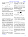
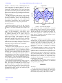
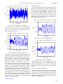
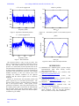
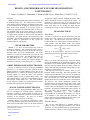
TUPSM029
Proceedings of BIW10, Santa Fe, New Mexico, US
DESIGN AND PERFORMANCE OF SSRL BEAM POSITION
ELECTRONICS*
J. Sebek#, D. Martin, T. Straumann, J. Wachter, SSRL/SLAC, Menlo Park, CA 94025, U.S.A.
Abstract
SSRL designed and built beam position electronics for
its SPEAR storage ring. We designed the electronics,
using digital receiver technology, for highly accurate turn
by turn measurements of both the position and arrival
time of the beam, allowing us to use this system to
measure the betatron and synchrotron tunes of the beam.
The dynamic range of the system allows us to measure
the properties of the beam at currents ranging from those
of single bunch injection to those of the full SPEAR
stored beam. This paper discusses the architecture of the
electronics, presents their performance specifications, and
shows a range of applications of this system for
accelerator physics experiments.
SPEAR PARAMETERS
SPEAR is a 3 GeV electron storage ring used for
synchrotron radiation. The operational beam current is
now 200 mA; the ring will run at 500 mA after all of the
beamline optics have been commissioned. The beam
emittance is 10 nm, the vertical beam size is 30 μm, and
the bunch length is 5 mm. The radio frequency (RF) of
the SPEAR klystron is 476.316 MHz and the ring
circumference is 234.3 meters; the harmonic number of
SPEAR is 372 and its revolution frequency is 1.28 MHz.
ORBIT FEEDBACK BPM ELECTRONICS
We use a modified version of the Bergoz MX-BPM
processor [1] to measure the beam position monitor
(BPM) signals for our orbit feedback system. We use 60
BPM processors to monitor the beam position and 60
steering magnets to correct the orbit. Our feedback
algorithm updates at a rate of approximately 4 kHz. Our
target orbit stability is 3 μm in a 1 Hz bandwidth, 10% of
the nominal vertical beam size. Our orbit feedback
system achieves a stability of a few hundred nm, an order
of magnitude better than our requirements.
SINGLE TURN BPM ELECTRONICS
We also wanted a high performance BPM processor
that was optimized for machine physics applications.
Therefore it needed to produce highly accurate turn by
turn data of the beam from which we could extract the
dynamics of the machine. We have 18 of these
electronics, one for each sector of the ring.
Machine physics use requires the electronics to work
over a large dynamic range, from injected beam to stored
beam at full current and it needs to work for all potential
___________________________________________
*Work supported by the U.S. Department of Energy under contract
number DE-AC02-76SF00515
#
[email protected]
Instrumentation
182
fill patterns, ranging from the standard fill pattern, when
almost all buckets are full, to single bunch studies. In
particular we need to be able to use this processor to
measure the betatron and synchrotron oscillations of the
beam, both when we are driving the beam and the
oscillations are strong, as well as when the beam is quiet.
BEAM SPECTRUM
Ideal Bunch
In order to motivate our system architecture, we first
briefly review the properties of a relativistic beam in a
storage ring. The ideal beam circles the ring at the
revolution period T. If the bunch were ultra-relativistic, a
point particle, and the BPM button had infinite
bandwidth, the signal would be a series of delta functions
( )=
( −
),
where Q is the bunch charge. Because of its periodic
nature the current can be expressed in a Fourier series
( )=
,
where
= 2 / , showing that the spectrum consists
only of the harmonics of the revolution frequency. Even
though there are an infinite number of harmonics, they all
carry the same information about the bunch. Finite size
of the bunch and finite bandwidth of the pickup give Q a
dependence on the frequency ω.
The ring may have up to h bunches, where h is the
harmonic number of the ring. The beam spectrum is still
composed of the harmonics of ω0, but now the amplitude
of the various harmonics depends on the fill pattern of the
ring. For example, if h is even, and every other bunch is
equally filled, only the coefficients of the even harmonics
are non-zero; one cannot distinguish between this
situation and one in which the ring is half as large (with
twice the revolution frequency) but in which every bunch
is filled. But even though there are an infinite number of
harmonics, the number of independent terms is finite. In
fact, since there are h bunches, there are only h
independent coefficients Qk.
The coefficient
corresponding to the klystron RF frequency ωRF, and all
of its multiples, is the same as the DC coefficient. In
order to obtain a signal independent of bunch pattern, one
needs to process the signal at a harmonic of ωRF.
Dynamic Bunch
We can see what happens to a dynamic bunch by
making a slowly varying approximation to the Fourier
expansion. A beam executing transverse motion about its
nominal trajectory will have a time-varying amplitude; a
Proceedings of BIW10, Santa Fe, New Mexico, US
beam executing longitudinal motion will have a timevarying phase. Therefore our Fourier expansion for a
dynamic beam is
( )=
( )
( )
where
( )=
( + ( ))
(
)is
and
the deviation in arrival time from the nominal
particle. Note that ( ) ≪ . We can therefore find a
mode of the beam motion by measuring the slowly
varying amplitude and phase of the beam. Betatron
oscillations are characterized as sinusoidal variations of
( ), corresponding to amplitude modulation, and
synchrotron oscillations are sinusoidal variations of ( ),
corresponding to phase modulation.
A beam with n bunches has n degrees of freedom.
Therefore, in order to measure all possible motions of the
beam, one needs to measure either n bunches in the time
domain or n harmonics (modes) in the frequency domain.
These are the methods used in feedback systems.
However, one can investigate the dynamics of a system
by driving one mode, the common mode ( = 0) in
which all bunches have the same motion, and observing
the beam response. The harmonics of ωRF correspond to
this common mode.
SIGNAL PROCESSING
We now know that we can obtain the information that
we want by extracting the information at ωRF and
measuring its slowly varying amplitude and phase. We
will digitize our data, resulting in a stream of digital data
to process. We now describe the signal processing
algorithm that we use on this data to achieve our goal.
Since we deal with a finite number of samples, our
processing involves a discrete filtering process. With the
appropriate choice of frequencies, and the appropriate
choice of our hardware architecture, we will see that this
filtering process is accomplished with a discrete Fourier
transform (DFT).
In general, it is very difficult to obtain the exact
information about one frequency from a DFT. This is
because a DFT has only finite resolution. It samples a
finite section of a waveform at N discrete, usually equally
spaced, times TS. The DFT assumes that this section of
length NTS repeats periodically. Therefore, since even a
pure sinusoid, in general, does not have an integral
number of periods during these N samples, the DFT does
not interpret this signal as a sinusoid, but rather as a
concatenation of identical sinusoidal segments. If the
sinusoid is not continuous in amplitude and slope, a cusp
arises in this infinite waveform. The DFT interprets this
cusp as higher frequencies that alias into a measured
frequency.
Only for a select set of problems can one construct the
system to avoid these problems and exactly measure the
frequency of interest. The beam signal from a storage
ring belongs to this set. As seen above, all of the
frequencies of interest are multiples of the revolution
Instrumentation
TUPSM029
harmonic ω0. If we sample for a period of time that is
= , then all of the
exactly one revolution period,
revolution harmonics have an integral number of
wavelengths during this period. The equally spaced
revolution harmonics are the orthogonal basis vectors of
the DFT.
In the frequency domain, the response of the DFT is a
series of sinc functions centered on the revolution
harmonics. The sinc amplitudes are unity at their central
harmonics and zero at the other harmonics. The DFT
separates out the different revolution harmonics to the
arithmetic precision of the digital processor.
The DFT produces a complex amplitude
( )
( )
for each harmonic during each revolution period; the real
part is the in-phase (I) signal component and the
imaginary part is the quadrature (Q) component. On each
revolution we use I and Q to calculate the magnitude
| ( )| =
+
and the phase
kω τ(t) = tan
of the revolution harmonic.
HARDWARE CONSIDERATIONS
Timing
In order to implement our system, we needed to
assemble a synchronous timing system that could support
the required timing infrastructure. Our system clock, fRF,
comes from a PTS-500 programmable frequency source
[2]. In addition to its low noise specifications, the PTS500 is phase continuous when its frequency is changed.
We need this property since fRF is part of our orbit
feedback system, we change it to correct for the diurnal
dispersion component of our orbit.
We then specified a frequency distribution chassis [3]
that generates from fRF all of our synchronous system
clocks. For the purposes of this article, the two
frequencies of interest are a local oscillator (LO) used in
the down-converter of the BPM and a digitizer clock.
The LO frequency, fLO, is exactly 359 times the revolution
frequency f0, so that our intermediate frequency (IF) will
be exactly 13f0. The system clock is 50f0. We use 50
samples per revolution to measure exactly 13 periods of
fIF.
(We also note that the sampling of our orbit feedback
BPM electronics is also synchronous with fRF. We sample
each of the multiplexed BPM buttons for exactly 80T0; a
complete module of four buttons is sampled every 320T0
which is almost exactly 250 µs. This is also the rate at
which our orbit feedback system calculates corrections
and at which the steering magnets update their
corrections.)
BPM Electronics Design
We designed, specified, and procured our hardware for
this system before the December, 2003 commissioning of
183
Proceedings of BIW10, Santa Fe, New Mexico, US
SPEAR3. At that time, 14 bit, 65 MSPS digitizers were
at the leading edge of commercial digitizers. The easiest
way to implement our DFT algorithm was to use a
commercially available digital receiver chip (subsequent
improvements in technology may now make the preferred
filter element an FPGA). We specified and purchased a
digital receiver (DR) board [4] and designed our own RFIF down converter.
The DR board supports eight channels of input, enough
for two BPM modules. Two programmable DR chips are
devoted to each channel. There is also on-board memory
that holds 128k samples for each channel; this
corresponds to approximately 100 ms of data capture,
much longer than the time of any beam phenomenon.
RF-IF Converter
Although the digitizers used in our DR board are
capable of direct RF sampling, there are many technical
advantages to first down-converting the RF signal to an
IF.
First, although the performance of the digitizer is still
good at fRF, the performance is even better at lower
≅ 16.645 MHz). Second, since there
frequencies (our
are technical limitations on the quality factors of
inexpensive band-pass filters, it is easier to construct
analog band-pass filters of the appropriate width at fIF
than at fRF.
Finally, the accuracy of the phase
measurement depends on the relative jitter of each clock
sample as measured in radians of the frequency to be
measured. By decreasing the frequency we process by a
factor of almost 30, we improve the phase accuracy of our
measurements by more than an order of magnitude.
Analog Signal Processing
Although we finally digitally process our signal, we
still need an analog signal processing stage to optimize
the system performance. We use a dielectric resonator
band-pass filter at fRF [5] to limit the peak voltage into our
electronics. Such commercial filters can achieve about a
1% bandwidth, so the length of the impulse response is
shorter than desired. These filters are periodic structures,
so although they reject very well frequencies near their
center frequency fC, they also pass higher harmonics of fC.
To reject these frequencies, we added a coaxial 600 MHz
low pass filter upstream of the electronics.
We performed our desired filtering at the IF, where we
built a Gaussian response filter with a bandwidth of 2
MHz. The response and bandwidth were chosen so that
an impulse response of a single bunch would provide
signal over the entire 50 samples of a single period T0 yet
decay without ringing before the next period.
Lengthening the impulse response also reduces the peak
amplitude seen by the digitizer.
Instrumentation
184
4
sampled data
x 10
2
1
amplitude
TUPSM029
0
-1
-2
0
20
40
60
sample
80
100
Figure 1: Two turns of IF samples
We used several stages of amplification. The gain
block in the RF stage was chosen for its low noise figure;
the one in the IF stage was chosen for its low distortion.
The RF gain block is used to amplify the signal for low
beam current applications. Both the RF gain block and
the IF filter are switchable so that the electronics can be
optimized for different applications.
Calibration
We chose to calibrate our system using a constant
calibration tone. We have combiners [6] located inside of
our ring, near the BPM modules, and there combine the
calibration tone with the signals from the beam. The
continuous signal allows us to avoid switches, so that we
do not have to skip data or compensate for switching
transients.
Our calibration frequency is chosen to be 1/2f0 below
fRF, well within the bandwidth of our analog stages. For
technical reasons, it is generated by a second frequency
synthesizer that is locked to the master synthesizer. (For
stability reasons, the tunes in a light source are always far
away from the half-integer.) In this mode, we have both
DR chips run on each channel and instead of producing a
measurement each revolution, we output data every
second turn. This allows the two signals to be orthogonal
to each other in the two DRs.
The calibration is only used during normal operation of
the BPM electronics with stored beam. It is turned off
during machine physics studies.
RESULTS
Accuracy
We first measure the accuracy of the BPM electronics
by examining the data for nominal user beam with a
standard fill. Figure 1 shows 100 samples, two complete
turns of data; the periodicity of the system is evident.
Proceedings of BIW10, Santa Fe, New Mexico, US
button 1 mean = 6581.7929 σ = 2.2804
6590
counts
6585
6580
TUPSM029
Spectral Purity
The spectral resolution of the horizontal beam position
measurement is displayed by the Fourier transform of the
turn by turn data displayed in Figure 5. The noise floor of
the measurement is approximately 115 dB below the
carrier, with spurs about 20 dB above this floor. All of
the tunes for a normal, quiet beam are clearly visible.
Again we see that the synchrotron tune is visible in the
horizontal beam spectrum; this is due to the BPM location
in a dispersive section of the ring.
6575
relative x position mean = -0.11212 σ = 0.00023
0
20
40
60
time (ms)
80
-0.1115
100
The data in Figure 2 is taken on a vacuum chamber
with a 17 mm half height. The standard deviation
measured for this 100 ms of data gives an accuracy of
about 7 µm per turn (781 ns).
Δ/Σ
Figure 2: Turn by turn data for one button.
-0.112
-0.1125
button 1 mean = 6581.7929 σ = 2.2804
6586
0
0.5
time (ms)
6584
Figure 4: First 1 ms of horizontal position.
counts
6582
phase stddev = 4.09 milliradians = 1.4 ps
6580
-0.51
6576
0
0.2
0.4
0.6
time (ms)
0.8
1
Figure 3: First 1 ms of turn by turn data.
However the standard deviation includes contributions
from beam motion, including synchrotron oscillations (in
dispersive regions) driven by transients in the klystron
high voltage power supply. If one instead measures σ
from the noise on the peaks of the synchrotron
oscillations in Figure 3, the resolution of each button,
before the position is calculated, is seen to be
approximately 1.4 µm per turn on a 34 mm high chamber.
We calculate the beam position using the standard
difference over sum calculation using the four buttons.
Figure 4, which shows the first ms of data shows that this
calculation improves the sensitivity of the measurement.
The phase measurement is also very accurate. Figure 5
shows that the standard deviation of the phase over 100
ms corresponds to 1.4 ps at ωRF. However, estimating the
σ from the noise at the top of the oscillations shows that
our accuracy is better than 100 fs. Note that, as expected,
the energy oscillations in Figure 4 are in quadrature with
the phase oscillations in Figure 5.
phase (radians)
6578
6574
1
-0.52
-0.53
-0.54
0
0.2
0.4
0.6
time (ms)
0.8
1
Figure 5: First 1 ms of bunch phase.
The horizontal tune line, only slightly visible in the
dense spectrum in Figure 6, is about 25dB above the noise
floor of the electronics, as seen in Figure 7. The vertical
and synchrotron tune lines are also very visible from the
spectra.
Low Current Injection Studies
Finally we look at data from low current injection
studies. A single bunch of current is injected into SPEAR
every 100 ms. In order to optimize injection, one needs to
determine that the phase delay between the injector and
SPEAR is correct and that the energy of the injected beam
matches the SPEAR energy [7].
Instrumentation
185
TUPSM029
Proceedings of BIW10, Santa Fe, New Mexico, US
x fft carrier suppressed
-60
-80
0.2
Δ/Σ
-100
dBC
relative x position
0.4
-120
0
-140
-0.2
-160
-180
0
200
400
frequency (kHz)
-0.4
600
νx (carrier suppressed)
Figure 8a:
beam.
-90
phase
4
phase (radians)
-110
dBC
100
Horizontal position of mis-timed injected
4.5
-100
-120
-130
-140
-150
3.5
3
2.5
134
136
138
frequency (kHz)
140
Figure 7: Horizontal tune.
The injected current is only 50 µA per pulse, four
orders of magnitude lower than the maximum current in
the ring. One cannot measure this low current in the
presence of a stored beam, but the injected beam can be
stored and then kicked out before the next injection cycle.
At these currents, the digitizer is at its bit resolution, but
the signal is still well above the noise floor. By averaging
multiple injections, in this case sixteen cycles were
averaged, the effective resolution of the digitizer
increases and the desired signals can be accurately
measured.
Figures 8a and 8b show the horizontal position and
phase, respectively of a mis-timed injected beam. The
position signal executes expected betatron oscillations
due to the injection kickers. Both signals execute
synchrotron oscillations. Since the position signal is sinelike and the phase signal is cosine-like, the injected beam
has the proper energy, but the incorrect phase. Proper
tuning of the injector phase reduces the measured phase
oscillation to ±0.1 radians.
Instrumentation
186
50
time (μs)
Figure 6: Spectrum of horizontal position.
-160
0
2
0
50
100
time (μs)
Figure 8b: Phase of mis-timed injected beam.
REFERENCES
[1] MX-BPM User’s Manual Spear-3 options, Bergoz
Instrumentation, Saint Genis Pouilly, France;
http://www.bergoz.com.
[2] Programmed Test Sources, Inc., Littleton, MA;
http://www.programmedtest.com.
[3] Wenzel
Associates,
Inc.,
Austin,
TX;
http://www.wenzel.com.
[4] Echotek Division of Mercury Computer Systems,
Huntsville, AL; http://www.mc.com.
[5] Integrated
Microwave,
San
Diego,
CA;
http://www.imcsd.com
[6] Mac Technology, Inc., Klamath Falls, OR;
http://www.mactechnology.com
[7] X. Huang, et al., “Optimization of the Booster to
Spear Transport Line for Top-Off Injection,”
PAC’09, Vancouver, May 2009, TU6RFP043.