Download Thesis - Institute For Systems and Robotics

Robotized Microscopy
Hugo Miguel Claro Pinto
Dissertação para obtenção do Grau de Mestre em
Engenharia Electrotécnica e de Computadores
Júri
Presidente:
Doutor Carlos Jorge Ferreira Silvestre
Orientador:
Doutor João Miguel Raposo Sanches
Co-Orientador:
Doutor José Miguel Rino Henriques
Vogal:
Doutor Andreas Miroslaus Wichert
Outubro 2009
To those who helped me obtaining everything I achieved so far.
i
ii
Acknowledgements
Despite the fact that a dissertation is an individual work there was some assistance and backup that
cannot and must not be forgotten.
First of all, I would like to take this opportunity to express my gratitude to professor João Sanches for
his guidance lines and his critical stimulus and recommendations during the realization of this project,
which where a fundamental contribution to the investigation.
I would also like to thank Doctor José Rino for all his general help and for supplying all the resources
needed and encouraging me to use them. I am specially thankful for his patience explaining me all
the basics of microscopy, and answering doubts that due to the lack of studies in this area sometimes
occurred to me.
My special regards also to engineer Ricardo Henriques who first introduced my to the microscopy field.
To all my course closest friends for their constant support and motivation especially in the hardest
moments.
Finally, but not by any means less important, I would like to thank my parents and brother for providing
me the conditions and encouragement to get this far, for their patience with me and without whom it
would not be possible to finish this work.
Thank you all!
Lisbon,
Hugo Pinto
October 2009
iii
iv
Abstract
This thesis proposes an alternative approach to the conventional microscopy research methods most
often found in biological research facilities. These methods involve an operator that constantly visualizes
and monitors the experiments’ environment, adjusting the microscope’s parameters as necessary.
The problem found during recent years to increase the autonomy level of microscopes lead to the
development of this thesis, which introduces a series of software libraries to control all the electronic
devices of the microscope. The introduction of a modular solution allows the possibility to use this
platform across different brands of microscopes, nonetheless maintaining the user interface. It also
allows the development of processing algorithms with almost full abstraction from the microscope
hardware in which they are implemented, giving portability to the system. In addition, this application
supports the possibility to use only some specific hardware components of the microscope instead of
the whole hardware setup, which permits controlling part of the microscope even if at some point some
hardware device has a breakdown.
The evaluation of the proposed system involved the development of a graphical user interface that
incorporates all the basic functionalities of every hardware device, to demonstrate the effectiveness
of the architecture proposed. Alongside, a visualization and image processing tool was developed
to present correctly all the captured data.
The obtained results suggest that the innovative visu-
alization/control method proposed in this work may yield significant benefits to the effectiveness of
microscopy research. In particular, the possibility of using this work to develop new algorithms capable
of controlling experiments in a fully automated manner. This dissertation also shows that the system
has increased functionality, ease of programmability and modularity over existing microscope control
software solutions and performs as well as the existing systems.
Keywords: Microscope, Microscopy, Automated, Modular Architecture, Teleoperation
v
vi
Resumo Analítico
Esta tese propõe uma abordagem alternativa aos métodos de investigação microscópica mais
frequentemente encontrados nas instalações de investigação biológica. Estes métodos envolvem um
operador que visualiza e monitoriza constantemente o ambiente experimental, ajustando os parâmetros
do miscroscópio quando necessário.
O problema encontrado nos últimos anos por forma a aumentar o nível de autonomia dos microscópios
levou ao desenvolvimento desta tese, que introduz um conjunto de bibliotecas de software para controlar
todos os dispositivos electrónicos do microscópio. A introdução de uma solução modular permite a
utilização desta plataforma em microscópios de diversas marcas, não obstante mantendo a interface
de utilizador. Permite também o desenvolvimento de algoritmos de processamento, com abstração total
do equipamento no qual são implementados, dotando o sistema de portabilidade. Além disso, esta
aplicação suporta a possibilidade de usar apenas alguns componentes de hardware do microscópio
ao invés de utilizar a configuração de hardware completa, o que permite controlar apenas parte do
microscópio, mesmo que em algum momento algum dispositivo de hardware sofra uma avaria.
A avaliação do sistema proposto envolve o desenvolvimento de uma interface gráfica de utilizador que
incorpora todas as funcionalidades básicas de cada componente de hardware, por forma a demonstrar
a eficácia da arquitectura proposta. Paralelamente, uma ferramenta para visualização e processamento
de imagem foi desenvolvida para apresentar correctamente os dados capturados.
Os resultados
obtidos sugerem que o inovativo método de visualização/controlo proposto neste trabalho possa render
benefícios significativos para a eficácia da investigação microscópica. Em particular, a possibilidade
de utilizar este trabalho para desenvolver novos algoritmos capazes de controlar experiências de modo
totalmente automático. Esta dissertação mostra também que o sistema aumentou a funcionalidade, a
facilidade de programação e a modularidade face às soluções de software de controlo microscópico
existentes e tem uma performance tão boa quanto estas.
Palavras-Chave: Microscópio, Microscopia, Automatizado, Arquitectura Modular, Teleoperação
vii
viii
Contents
1 Introduction
1
1.1 Robotized Microscopy: Towards a more accurate examination . . . . . . . . . . . . . . . .
1
1.2 Context and Overview . . . . . . . . . . . . . . . . . . . . . . . . . . . . . . . . . . . . . .
2
1.3 State of the art . . . . . . . . . . . . . . . . . . . . . . . . . . . . . . . . . . . . . . . . . .
3
1.4 Dissertation aim and objectives . . . . . . . . . . . . . . . . . . . . . . . . . . . . . . . . .
6
1.5 Dissertation structure . . . . . . . . . . . . . . . . . . . . . . . . . . . . . . . . . . . . . .
8
2 System Architecture
9
2.1 Microscope overview . . . . . . . . . . . . . . . . . . . . . . . . . . . . . . . . . . . . . . .
9
2.2 Proposed architecture . . . . . . . . . . . . . . . . . . . . . . . . . . . . . . . . . . . . . .
13
2.2.1 Overview of the system’s modus operandi . . . . . . . . . . . . . . . . . . . . . . .
14
2.3 Existing Layers . . . . . . . . . . . . . . . . . . . . . . . . . . . . . . . . . . . . . . . . . .
16
2.4 Developed Layers . . . . . . . . . . . . . . . . . . . . . . . . . . . . . . . . . . . . . . . .
16
2.5 Software tools
18
. . . . . . . . . . . . . . . . . . . . . . . . . . . . . . . . . . . . . . . . . .
3 Hardware Devices
3.1 Camera Module
21
. . . . . . . . . . . . . . . . . . . . . . . . . . . . . . . . . . . . . . . . .
24
3.1.1 Motivation . . . . . . . . . . . . . . . . . . . . . . . . . . . . . . . . . . . . . . . . .
24
3.1.2 Implementation . . . . . . . . . . . . . . . . . . . . . . . . . . . . . . . . . . . . . .
24
3.1.2.1
Communication: Initializing the module . . . . . . . . . . . . . . . . . . .
24
3.1.2.2
Capturing images . . . . . . . . . . . . . . . . . . . . . . . . . . . . . . .
27
3.1.2.3
Region of Interest . . . . . . . . . . . . . . . . . . . . . . . . . . . . . . .
29
3.1.2.4
Binning Factor . . . . . . . . . . . . . . . . . . . . . . . . . . . . . . . . .
30
3.2 Prior Module . . . . . . . . . . . . . . . . . . . . . . . . . . . . . . . . . . . . . . . . . . .
33
3.2.1 Motivation . . . . . . . . . . . . . . . . . . . . . . . . . . . . . . . . . . . . . . . . .
33
3.2.2 Implementation . . . . . . . . . . . . . . . . . . . . . . . . . . . . . . . . . . . . . .
34
ix
C ONTENTS
3.2.2.1
Communication . . . . . . . . . . . . . . . . . . . . . . . . . . . . . . . .
34
3.2.2.2
Stage device . . . . . . . . . . . . . . . . . . . . . . . . . . . . . . . . . .
35
3.2.2.3
Filter wheel . . . . . . . . . . . . . . . . . . . . . . . . . . . . . . . . . . .
39
3.3 Uniblitz Module . . . . . . . . . . . . . . . . . . . . . . . . . . . . . . . . . . . . . . . . . .
41
3.3.1 Motivation . . . . . . . . . . . . . . . . . . . . . . . . . . . . . . . . . . . . . . . . .
41
3.3.2 Implementation . . . . . . . . . . . . . . . . . . . . . . . . . . . . . . . . . . . . . .
41
3.3.2.1
Communication . . . . . . . . . . . . . . . . . . . . . . . . . . . . . . . .
41
3.3.2.2
Shutter functions . . . . . . . . . . . . . . . . . . . . . . . . . . . . . . . .
41
3.4 Zeiss Module . . . . . . . . . . . . . . . . . . . . . . . . . . . . . . . . . . . . . . . . . . .
43
3.4.1 Motivation . . . . . . . . . . . . . . . . . . . . . . . . . . . . . . . . . . . . . . . . .
43
3.4.2 Implementation . . . . . . . . . . . . . . . . . . . . . . . . . . . . . . . . . . . . . .
44
3.4.2.1
Communication . . . . . . . . . . . . . . . . . . . . . . . . . . . . . . . .
44
3.4.2.2
Focus device . . . . . . . . . . . . . . . . . . . . . . . . . . . . . . . . . .
45
3.4.2.3
Selectable states of operation . . . . . . . . . . . . . . . . . . . . . . . .
47
3.4.2.4
Internal shutter . . . . . . . . . . . . . . . . . . . . . . . . . . . . . . . . .
48
3.5 Micro-Manager: Core Services Module Layer . . . . . . . . . . . . . . . . . . . . . . . . .
50
3.5.1 Loading the system configuration properties . . . . . . . . . . . . . . . . . . . . . .
51
3.5.2 Accessing the Core functionalities . . . . . . . . . . . . . . . . . . . . . . . . . . .
52
4 Evaluating the application
55
4.1 A visualization toolkit . . . . . . . . . . . . . . . . . . . . . . . . . . . . . . . . . . . . . . .
55
4.2 Developing a GUI . . . . . . . . . . . . . . . . . . . . . . . . . . . . . . . . . . . . . . . . .
57
4.2.1 Linking the necessary libraries . . . . . . . . . . . . . . . . . . . . . . . . . . . . .
58
4.2.2 Connecting the Interface to the devices . . . . . . . . . . . . . . . . . . . . . . . .
59
4.2.3 Writing the configuration file . . . . . . . . . . . . . . . . . . . . . . . . . . . . . . .
59
4.2.4 Coordinates system . . . . . . . . . . . . . . . . . . . . . . . . . . . . . . . . . . .
60
4.2.5 The stage and focus controllers . . . . . . . . . . . . . . . . . . . . . . . . . . . . .
61
4.2.6 Camera Settings . . . . . . . . . . . . . . . . . . . . . . . . . . . . . . . . . . . . .
62
4.2.7 Shutter settings . . . . . . . . . . . . . . . . . . . . . . . . . . . . . . . . . . . . . .
63
4.3 Results and evaluation . . . . . . . . . . . . . . . . . . . . . . . . . . . . . . . . . . . . . .
63
5 Conclusion
65
5.1 Future work . . . . . . . . . . . . . . . . . . . . . . . . . . . . . . . . . . . . . . . . . . . .
A Microscope Devices datasheets
65
67
x
C ONTENTS
A.1 Objectives datasheet . . . . . . . . . . . . . . . . . . . . . . . . . . . . . . . . . . . . . . .
67
A.2 Filters sets datasheet . . . . . . . . . . . . . . . . . . . . . . . . . . . . . . . . . . . . . .
73
B Core functions
75
C Configuration File
81
xi
C ONTENTS
xii
List of Tables
2.1 Carl Zeiss Objectives Information. . . . . . . . . . . . . . . . . . . . . . . . . . . . . . . .
10
2.2 Zeiss Filter Sets Information. . . . . . . . . . . . . . . . . . . . . . . . . . . . . . . . . . .
10
3.1 Camera Device Properties. . . . . . . . . . . . . . . . . . . . . . . . . . . . . . . . . . . .
26
3.2 Stage XY maximum resolution. . . . . . . . . . . . . . . . . . . . . . . . . . . . . . . . . .
34
3.3 Prior Serial Port settings. . . . . . . . . . . . . . . . . . . . . . . . . . . . . . . . . . . . .
34
3.4 Shutter connection parameters. . . . . . . . . . . . . . . . . . . . . . . . . . . . . . . . . .
41
3.5 Prior Serial Port settings. . . . . . . . . . . . . . . . . . . . . . . . . . . . . . . . . . . . .
45
3.6 System Configuration. . . . . . . . . . . . . . . . . . . . . . . . . . . . . . . . . . . . . . .
53
4.1 Image visualization and processing functions. . . . . . . . . . . . . . . . . . . . . . . . . .
56
4.2 A 12-bit to 16-bit conversion example. . . . . . . . . . . . . . . . . . . . . . . . . . . . . .
57
xiii
L IST OF TABLES
xiv
List of Figures
1.1 Examples of microscopy applications. . . . . . . . . . . . . . . . . . . . . . . . . . . . . .
6
2.1 Zeiss Axiovert 200M. . . . . . . . . . . . . . . . . . . . . . . . . . . . . . . . . . . . . . . .
12
2.2 System architecture. . . . . . . . . . . . . . . . . . . . . . . . . . . . . . . . . . . . . . . .
13
2.3 System modus Operandi. . . . . . . . . . . . . . . . . . . . . . . . . . . . . . . . . . . . .
15
2.4 Devices interface connector. . . . . . . . . . . . . . . . . . . . . . . . . . . . . . . . . . . .
17
3.1 Camera initialization. . . . . . . . . . . . . . . . . . . . . . . . . . . . . . . . . . . . . . . .
25
3.2 Camera settings initialization. . . . . . . . . . . . . . . . . . . . . . . . . . . . . . . . . . .
27
3.3 Camera’s acquisition processes. . . . . . . . . . . . . . . . . . . . . . . . . . . . . . . . .
28
3.4 Example of a ROI selection. . . . . . . . . . . . . . . . . . . . . . . . . . . . . . . . . . . .
30
3.5 Binning example. . . . . . . . . . . . . . . . . . . . . . . . . . . . . . . . . . . . . . . . . .
31
3.6 Binning noise caption example. . . . . . . . . . . . . . . . . . . . . . . . . . . . . . . . . .
31
3.7 Stage initialization process. . . . . . . . . . . . . . . . . . . . . . . . . . . . . . . . . . . .
35
3.8 Diferences between the operator and the objectives frames. . . . . . . . . . . . . . . . . .
36
3.9 Stage User Interaction.
. . . . . . . . . . . . . . . . . . . . . . . . . . . . . . . . . . . . .
38
3.10 Wheel Algorithm. . . . . . . . . . . . . . . . . . . . . . . . . . . . . . . . . . . . . . . . . .
40
3.11 Focus sequence of operations. . . . . . . . . . . . . . . . . . . . . . . . . . . . . . . . . .
46
3.12 User interaction with devices of predefined states of operation. . . . . . . . . . . . . . . .
47
4.1 Graphical user interface. . . . . . . . . . . . . . . . . . . . . . . . . . . . . . . . . . . . . .
57
4.2 Linking the libraries with the GUI. . . . . . . . . . . . . . . . . . . . . . . . . . . . . . . . .
58
4.3 Time-lapse graphical display . . . . . . . . . . . . . . . . . . . . . . . . . . . . . . . . . .
63
A.1 Filter sets characteristics. . . . . . . . . . . . . . . . . . . . . . . . . . . . . . . . . . . . .
73
xv
L IST OF F IGURES
xvi
List of Acronyms
OSS
-
Open Source Software.
GUI
-
Graphical User Interface.
HD
-
High-Definition.
OpenCV
-
Open Source Computer Vision Library.
NA
-
Numerical Aperture.
CCD
-
Charge-Coupled Device.
PVCAM
-
Programmable Virtual Camera Access Method.
SDK
-
Software Development Kit.
ROI
-
Region Of Interest.
OS
-
Operating System.
DLL
-
Dynamic-link library.
RMS
-
Root Mean Square.
DIC
-
Differential Interface Contrast.
PCI
-
Peripheral Component Interconnect.
IPL
-
Image Processing Library.
ACE
-
ADAPTIVE Communication Environment.
USB
-
Universal Serial Bus.
MFC
-
Microsoft Foundation Classes.
BP
-
Band Pass.
LP
-
Long Pass.
FT
-
Fourier Transform.
xvii
L IST OF F IGURES
xviii
C HAPTER 1
Introduction
1.1
Robotized Microscopy: Towards a more accurate examination
Around the year 1590 the first optical microscope - an instrument capable of enabling the human eye,
by means of a lens or combinations of lenses, to observe enlarged images of objects that are too small
to be seen by unaided eye - was built and with it the possibility of discovering worlds within worlds was
born. Since that time microscopy - a scientific discipline employing the use of microscopes to magnifying
objects - has seen an increasingly and notorious importance in everyone’s life. It is used in a wide range
of applications, especially in the biology field where it is an essential tool for researchers, indirectly
bringing major advances to medicine and people’s health.
Due to the small dimensions of most of the studied organic and/or inorganic entities, urges an imperative
need of sophisticated devices being able to clearly present those entities, allowing the researchers
to properly analyze them. Thus, currently microscopes are developed with the goal of providing the
necessary tools to enhance the details on the samples, so that they may be studied more accurately. To
heighten image details, all microscopes are developed taking three basic concerns into account:
• produce a scaled up image of the specimen, to be able to see more detail, maintaining the image
perspective (magnification);
• increase the details in the observed image, i.e., resolution augmentation;
• emphasize the image contrast either to the human eye as to cameras devices.
In current microscopy, when an individual needs to analyze or collect images of specimens he has
to pay constant attention to a whole set of variables introduced by the system, especially if taken into
consideration that, in the last decades, the study of living specimens has seen a notorious growth raising
major interests to the biological research community. Whereas handling living cells, the cells’ movements
need to be supervised to avoid losing their track, especially for long time exposure experiments, and
therefore avoid losing the events of interest to be captured during the experiments. Consequently, with
the presently available technology the operator must be physically present at the experiment’s location,
at least with some regular frequency, to control the parameters of the microscope, mainly the stage
1
C HAPTER 1: I NTRODUCTION
movements, the focus and the magnification adjustments.
Although being a fairly simple task for an experienced researcher, it can also be an exhausting one,
taking into account that experiments may, not rarely, last for several hours. Moreover, researchers have
to take into account that several other devices of the microscope may also need to be periodically
operated.
Under these conditions, the need for solutions with the purpose of augmenting the instrumentation’s
autonomy is imperative not only to the manufacturers of the microscopes but also to the researchers
that use those microscopes. Regarding this concern, over the last decades microscopy has known a
massive increase in the use of electrical technology, allowing not only better immediate results due to
the greater quality of the equipment, but also to overcome analysis obstacles through the insertion and
merging of the automation field into the microscopy field [1–3].
1.2
Context and Overview
Recent years have seen a massive growth and advance in microscopy technology. Thereby research
centers had replaced their old and traditional microscopes with new electrical and fully automated ones.
Almost all the basic components of an electrical microscope are nowadays also electric and capable
of being remotely operated. This fact has potential to bring major advances in microscopy research,
making the emerging software control solutions and its associated hardware to become an essential
part of the biological research.
However, this new business opportunity led to almost all the microscopes manufacturers and its
associated peripherals starting to produce their own commercial software solutions to increase their
profits. Such a competition has considerably increased the number of technical incompatibilities between
the hardware devices and the software solutions, and even when working with hardware and software
from the same manufacturer it is not rare to find such a phenomenon. Thus, biological researchers
find themselves with the problem of taking full advantage of automated microscopes, since the existing
software packages are not as generic as they should be and mainly are not easy-to-use.
It becomes clear that in the microscopy industry it should be required a generic system, able to easily
incorporate several microscope components from different manufacturers, without compatibility issues.
This software would provide a basis of support to subsequent developed applications. Moreover, once
a generic but fully automated system is build several improvements are possible to be made, leading to
significant changes in current microscopy approaches.
A significant change is the possibility of allowing a researcher to see and control its experiments without
being physically present at the laboratory location. D. Loureiro [4] has been developing a system
integrating the architecture developed on this dissertation and the Internet services, with the purpose of
being therefore used to operate the microscope through the Internet.
The usefulness of this technology becomes clear even for a very simple situation as the following:
acquiring images of a living sample in certain periods of time for several hours. Although current
microscope control systems already enable automation of some of the motorized components, image
acquisition is only allowed for fixed-time lapse at predetermined positions. However, events of interest
occur stochastically and in a time interval that may long for several hours. Therefore, such conventional
2
C HAPTER 1: I NTRODUCTION
approaches may prove to be insufficient or inadequate, since successful image acquisition implies the
generation of amounts of data largely exceeding the necessary, which will need to be filtered afterwards
to remove the undesired events. This situation causes time consuming tasks to be performed after
the acquisition, and mostly important, does not guarantee that the set of captured images contain the
desired events of interest.
Nonetheless, with a fully automated system like the one proposed in this dissertation and the work
developed by D. Loureiro it is possible to analyze the cells and control the microscope in real-time
without having to be physically present at the experiment, and therefore is possible to adjust dynamically
the experiment’s parameters, maximizing the number of images containing events of interest and
simultaneously minimizing the amount of data captured. Using this solution the researcher has control
over all the electrical devices, and also the possibility to set the camera in live imaging mode (i.e.
streaming mode) to view the experiment’s evolution in real-time and make the necessary adjustments to
all the other microscope’s devices.
An aspect that becomes immediately obvious is that Internet microscopy [5] (hereafter named
telemicroscopy) offers a new set of possibilities for microscopy analysis, as the use of this technology
should promote communication between researchers, endowing every researcher with an Internet
connection to access the acquired images or acquiring new images, and allowing them to crosscheck
diagnosis, increasing its quality. On the other hand, the time it takes for medical clinics to receive images
at off-site laboratories is also suitable of being reduced and their medical staff is also given the ability to
control the process of acquiring images from the microscope to further analyze the results.
Another improvement that may be added to microscopy, with a huge spectrum of implementation, is
the use of other research areas, such as image/signal processing tools, to analyze the experiments’
data before its acquisition and by that means guarantee better results. Although image processing is
already used in microscopy nowadays it is not made in real time, i.e. currently the data is acquired
and the processing analysis is made after the experiment is ended. Often this processing is also made
to enhance the captured images properties, due to a poor acquisition process. Thereby, it becomes
notorious the major advantages that using such tools prior to the data acquiring process would bring,
since the system is able to discard the lower quality data and repeat the acquisition until the results have
the quality demanded (or at least the best quality possible when the demanded quality is not reachable).
1.3
State of the art
The usage of automation software packages in microscopy field is not an entirely new process. In truth,
over the last decade it has known a tremendous boost, with the marketing of solutions to control some of
the electrical microscope’s devices. However, those solutions are very expensive, and most of the time
incompatible with each others. Nonetheless, it is not possible to add new functionalities to the software,
with the researchers being limited to the already existing ones.
Another common aspect is that most of the available applications focus on image acquisition, image
analysis or image reconstruction. In fact, the currently available software packages are essentially
developed to handle image quality enhancement at a later stage of the image capturing phase. Hence,
there are not many packages handling and processing images previous to the acquisition process,
3
C HAPTER 1: I NTRODUCTION
enhancing the acquired image quality by natural means (i.e. adjusting the capture parameters) and
not through algorithmic processes (which many times induce artificial characteristics to the data). Also,
while some software packages provide a set of tools to endow the use of algorithms in several different
structural problems, others were designed to provide a set of tools optimized for a particular structural
problem. However, generally the more generic a software package is the less effective the results are,
meaning that a trade-off between quality of the results and portability of the application is a significant
factor.
Regarding the latest advances in technology another recent application is the development of software
tools enabling researchers to acquire three-dimensional images and three-dimensional time series
of images [6]. These commercial solutions overcome the microscope’s constraints, acquiring twodimensional images closely spaced into a stack and after use the software to manipulate the stack
and handle it as single three-dimensional image.
Other commercial software solutions, with MetaMorph
1
[7] becoming one of the most widespread
and commonly used, are evolving towards complete hardware solutions
2
integrating both the imaging
software (for automated image acquisition and processing) and the microscope’s peripherals automated
control. Regarding this issue, MetaMorph is optimized for multi-dimensional experiments, enabling the
control of the illumination, the lens magnification and the XY stage and z-focus axis location settings,
alongside with a customizable auto-focus feature maintaining in focus long time events, whenever the
hardware devices can be remotely operated. Also, Metamorph’s automation features, such as image
stacks, were designed enabling the ability to process data sets containing hundreds of images and
handling large amounts of information.
Axiovision 3 [8], is a digital image processing software, granting the possibility to control all microscope’s
parts developed by Carl Zeiss manufacturer, among which are digital cameras, objective’s turrets,
motorized stages, or filter wheels. Similar to other solutions, Zeiss developed its own image storing
solution, named the Carl Zeiss ZVI image: a file format developed specifically for scientific microscopy
where along with the image additional information about the experiment is stored (the capturing time,
the spatial position, the lens magnification, etc).
There are also available some freeware solutions, and between those solutions there is one that
begins to be accepted as the most commonly used platform, named Micro-Manager
4
[9] [10], mostly
because of its flexibility and unrestricted modifications and extensions of the functionalities, not only
due to the device support licensing, but also due to an extremely active support community that is
constantly upgrading the application. Micro-Manager OSS platform is designed for imaging and control
of automated microscopes working on multiple platforms like Windows, Linux and Mac. To understand
the advantages of this solution it must be highlighted the application is based on a modular architecture,
supported on a three independent layers structure [9]:
• DA (Device Adapters) - the communication between the different devices and the application is
made using this layer. Hence, according to the specific hardware configuration the adapters held
by this layer differ.
1 http://www.moleculardevices.com/pages/software/metamorph.html
2 http://www.moleculardevices.com/pages/software/metamorph_acquisition.html
3 http://www.zeiss.com/axiovision
4 http://micro-manager.org
4
C HAPTER 1: I NTRODUCTION
• CSM (Core Services Module) - olds not only hardware abstraction allowing the system functionalities to work independently of the microscope, but also all the necessary functions to allow a
researcher to call and access a desired DA. The CSM controls and synchronizes all the microscope
devices operations (camera, stage, shutters, etc.), granting also access to the application from
many different programming environments (C++, Java, Matlab, Python, Perl and others).
• GUI - a user graphical interface incorporates the CSM functionalities developed in C++ and
wrapped in a Java layer, making them visually user friendly and ease-of-use.
Hence, a comparison between Micro-Manager and the other available solutions highlights the modular
structure of Micro-Manager and therefore its possibility of adapting the system to the hardware
configuration by simply changing the DA layer controllers’ configuration.
As to telemicroscopy, the emergence and usage of this new concept has been rapidly increasing in
distinct areas [11, 12], as an auxiliary tool to a better and more accurate diagnosis. The system is
usually based on a common client-server application with two major components: the server component,
consisting of a computer with Internet access connected to the automatic microscope by some software
control application; the client component, consisting of an Internet browser or a dedicated application
to remotely operate the microscope. The purpose of this system is to transform the microscope into an
Internet server application endowing all the connected clients to operate it remotely and simultaneously.
Notwithstanding, one of the best examples of how the Internet services can be used to operate a
microscope is presented by Iver Petersen et al. [5, 11]: A.M.B.A. 5 authors developed a telemicroscopy
system based on a client-server application, with the server being a computer with Internet access
connected to an automated microscope via Java based software, and the client a computer with Internet
access and a web browser with Java support, which allows the possibility to connect several clients to
the microscope, superimposing their experiment’s diagnosis and cross-referencing online information
using a system Chat function and forming a network for teleconsultation.
iPath-Microscope
6
is another example of telemicroscopy software, developed to be integrated by
hospitals to perform intra-operative diagnosis and second opinion consultations in the pathology field.
This application integrates two different main functionalities et al. [12]: the control of a remote microscope
(with, at least the possibility of transferring images from the microscope to the researcher) and a
database for the storage of several aspects like the patients’ data, information collected from each
session, images collected from the experiments, etc. However, this application is limited both in the
number of features that provides the user, as well as the compatibility with different brands of hardware
manufacturers.
Finally, NCMIR
7
researchers developed and presented a telemicroscopy system
8
et al.: the system
provides a Web-based access to the JEOL 4000EX IVEM - one of the few intermediate high-voltage
electron microscopes available to the biological research community in the United States - through a user
interface called VidCon, implemented in Java programming language and runnable on any Java-capable
Web browser. This interface displays the microscope’s optical and stage parameters and a live video
5 http://amba.charite.de/
6 http://www.ipath.ch/site/telemicroscopy
7 http://ncmir.ucsd.edu/press/06_korea_ncmir.shtm
8 https://ftp.isoc.org/inet2000/cdproceedings/5a/5a_4.htm
5
C HAPTER 1: I NTRODUCTION
image of the specimen under examination. Also, all participants can view the results of commands and
the images acquired, although only the user in control of the instrument is allowed to send commands
to it. It is also possible to share information promoting interaction among the session’s participants. At
the microscope site, a workstation acts as the Web server and the video server, while other workstation
is used to control and communicate with the microscope and associated image-processing hardware.
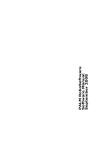
Figure 1.1 shows several of the telemicroscopy applications interfaces and communication processes
mentioned above.
(a) Metamorph Interface
(b) Micro-Manager Interface
(c) AMBA interface.
(d) NCMIR interface.
Figure 1.1: Examples of microscopy applications.
1.4
Dissertation aim and objectives
The developed work is concerned on providing a generic and easy-to-use prototype platform to be
straightforwardly used and also customized according to the researchers needs. This prototype sets
control of all the microscope’s devices, and allows the researcher to easily incorporate or remove a
single or multiple devices. Hence, new functionalities can be easily incorporated in the solution and the
existing ones modified.
6
C HAPTER 1: I NTRODUCTION
A solution systematized for the goal of creating a microscope control system despite of the manufacturer
seems unrealistic, as a control solution implies specific hardware and not general. To overcome that
issue, an approach to divide the general problem into smaller problems is used. Factoring the initial
abstract point at issue into smaller and more specific problems, makes it easier to define and focus on
the several demands to solve these concrete difficulties.
Alongside with the proposed novel microscope control automation tools this work aims at incorporating
and providing also a set of data processing tools that can be applied by the biological research units to
fulfill their needs for advanced microscopy techniques, endowing them with the necessary instruments
to develop their own applications to solve specific problems.
The urge for data processing tools became perceptible whereas most of the currently available control
systems present significant image acquisition constraints and therefore the development of these tools
should be driven by key biological questions for which the currently available solutions are proved to be
insufficient or inadequate. A simple example are phenomena like photobleaching and photodamage,
capable of being reduced simply through the introduction of data processing tools in the application to
analyze the acquired data and use this information to control the microscope.
Concluded the stages of development regarding the conception of fully functional controllers for the
whole set of devices and endowing the researcher with a full set of processing tools, the third part of this
thesis is dedicated on using the developed platform to bring a new concept to the microscopy studies:
the control of a microscope over the Internet.
This is a completely innovate field, and due to the major advantages and contribution that can provide
to the researchers studies, it is imperative not only to have a fully stable and reliable system but also a
system that guarantees the maximum accuracy of the microscope’s devices.
Therefore, comparing the work proposed in this dissertation to the commercial available solutions
immediately outlines several differences stressing the advantages of the proposed work, mainly in the
image acquisition process, whereas most of the currently available control systems only allow sequential
image acquisition at predetermined stage and focus positions with fixed time-lapse.
Beyond the features constraints and lack of flexibility of the currently available solutions are also
logistics issues that research laboratories must take into consideration at the moment of choosing and
purchasing software solutions to use, especially considering the extremely high costs associated to
microscopy software that generally forbids the regular purchases of newly improved software packages.
Furthermore, commercial solutions are, often designed to work restrictly with some hardware brands
and therefore incompatible to work with equipment provided by other manufacturers and being able to
control all the microscope’s hardware devices frequently requires the use of more than one application
simultaneously.
Hence, the motivation to provide a generic and easy-to-use prototype platform capable of being
customized to work in all the robotized microscopes within a research unit, providing not only a common
application to all the researchers enhancing their knowledge of the software, but also a financially viable
solution.
It should be outlined that at this early phase of development the proposed work is not meant to replace
the current on site visualization and control system, but rather to complement it. However, future
upgrades on the microscope hardware devices that are still not electronically controlled could easily lead
to the development of all the necessary control tools, making an Internet visualization/control system the
7
C HAPTER 1: I NTRODUCTION
only requirement during an experiment.
It should also be emphasized that this work does not aim on building a platform to compete with the
currently available solutions on the market, but rather to develop a set of tools that consist on a major
basis to endow future researchers to build their own customizable sets of intelligent algorithms. These
tools give researchers the potentialities of taking microscopy studies and cells analisis into a completely
new deepening level than the currently available solutions allow, consequently allowing the usage of new
techniques.
1.5
Dissertation structure
This dissertation is organized in the following structure:
• Chapter 2: System Architecture - The system hardware is presented and the general system
architecture, used to implement the main goals, is explained. The modular software architecture
is explained and the developed layers and control modules are described and justified.
• Chapter 3: Hardware Devices - Chapter 3 goes into detail explaining the software developed to
control all the electrical/motorized hardware devices.
• Chapter 4: Evaluating the application - An example of a user interface is shown to explain how
to integrate the several features of this architecture and to test its performance. The necessary
image processing tools are developed, explained and integrated in the user interface.
8
C HAPTER 2
System Architecture
In this chapter, the general equipment specifications are described and an overall system architecture is
introduced followed by a preview of the existing and the proposed modules of that architecture. Finally,
the software tools used during the development of this thesis are mentioned.
2.1
Microscope overview
The microscope targeted for this dissertation is located at the Instituto de Medicina Molecular (IMM)
and the developed work is a direct result of a currently underway collaboration between the Institute of
Systems and Robotics (ISR) of Instituto Superior Técnico (IST) and the BioImaging Unit of Instituto de
Medicina Molecular.
The equipment used consists of an Axiovert 200M, a completely motorized wide-field inverted
microscope developed by Zeiss manufacturer [13, 14]. Within the equipment manufactured by Zeiss
are also the objectives, the objective’s turret, the motorized z-focus, the reflector’s turret, the Optovar
magnification lens, the camera port, the halogen lamp and the mirrors system to direct the light beams.
Alongside with the microscope other major components are used: a Roper Scientific cooled camera [15],
a high precision two-dimensional stage and a filter wheel both developed by Prior Scientific [16], a
UniBlitz shutter [17] and an ordinary personal computer (hereafter named as console).
The Zeiss Axiovert 200M is a robust electric microscope built for specimens examination in transmitted
and reflected light, ideally developed for commercial use in the following applications [18]:
• Structure and surface analysis;
• Particle and granule size analysis;
• Pore and crack testing.
It can be used for bright-field, DIC (Differential Interference Contrast), epi-fluorescence and phase
contrast and techniques.
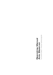
The main features of this microscope, depicted in Figure 2.1 [13], are the following:
9
C HAPTER 2: S YSTEM A RCHITECTURE
• Objectives and objectives turret:
The most important optical components of a microscope are the objectives, forasmuch as the
objectives arbitrate the quality of the images acquired, gathering the light passing through the
sample and then projecting an accurate and real image back into either an eyepiece 1 or a camera.
A motorized nosepiece
2
designed for HD DIC - an illumination technique used to enhance the
contrast in unstained and transparent samples [18] - with six predefined positions for placing the
objectives makes the microscope adaptable to a wide range of requirements.
Table 2.1 presents the main features of the Carl Zeiss objectives currently placed on the turret and
used during this work (the product sheet can be found in Appendix A.1).
Table 2.1: Carl Zeiss Objectives Information.
Position
Magnification
Class
Type
NA
10 um (pixels)
0
10x
Plan-Neofluar
Air
0.30
10
1
20x
Plan-Apochromat
Air
0.80
21
2
40x
EC-Plan-NeoFluar
Air
0.75
41
3
63x
Plan-Apochromat
Oil
1.40
65
4
100x
Plan-Apochromat
Oil
1.40
102
5
none
• Filters and filters turret:
A motorized turret accepting a maximum of five modules of reflectors for epi-fluorescence (the
excitation and observation of the fluorescence are from above the specimen). Table 2.2 presents
the main features of the sets of filters present on turret (the product sheet can be found in
Appendix A.2).
Table 2.2: Zeiss Filter Sets Information.
Position
Filter Set
Excitation (nm)
Emission (nm)
Beam Splitter (nm)
0
Filter Set 01
BP 359-371
LP >397
FT 395
1
Filter Set 09
BP 450-490
LP >515
FT 510
2
Filter Set 10
BP 450-490
BP 515-565
FT 510
3
Filter Set 15
BP 540-552
LP >590
FT 580
4
Ablation
none
none
none
• Optovar Magnification:
A motorized tubelens turret allowing three different magnification factors: tubelens 1.0x, optovar
lens 1.6x and optovar lens 2.5x. This magnification lens combined with the objective’s magnification and the eyepiece magnification (in case the researcher is observing through the eyepiece)
gives the total image magnification.
1 The
2 The
tub lens attached to the microscope for looking at the sample.
rotating part of the microscope that holds the objectives.
10
C HAPTER 2: S YSTEM A RCHITECTURE
• Illumination:
The transmitted light source is granted by a 100W halogen lamp. However, although the lamp
intensity is electronically controlled, according to the manufacturer it was not developed a hardware
controller to set the lamp intensity by software. Therefore, it was not possible to develop a software
controller for this device.
The fluorescence light source is powered by an ebq100 isolated power supply.
• Substage Condenser:
The substage condenser converges light from a light source into a cone to illuminate the sample,
through a lens designed to converge the light to a focus at a back focal plane of the objective, and
an aperture that blocks out a variable undesired amount of light.
Although Zeiss Axiovert 200 M is supposed be equipped with a motorized condenser with a six
positions turret for placing the lens, the microscope at IMM does not have its original condenser
installed and a manually handled one is used instead. For this reason, is was not possible
to develop a controller for the light condenser and the sample illumination has to be manually
converged.
• Focus device:
A precise focus axis is of extreme importance for the quality of the images acquired, since
the quality of the contrast observed in the image is intrinsically related to the accuracy of the
focus system. Regarding this issue, a motorized harmonic drive, ensures a minimum step size
movement of 25 nm along the focus axis (hereafter also named the Z axis direction).
• Roper Scientific camera:
The image acquisition process is ensured by a Photometrics CoolSnap HQ model camera
developed by Roper Scientific, a monochromatic cooled CCD camera developed for low-light
scientific and industrial microscopy. Cooling the CCD improves its sensitivity to low light intensities
reducing the dark current and hence the thermal noise. In this model, the dark current responsible
for adding dark noise to the image, is minimized below 0.05 e-/pixel/sec.
Alongside, a progressive scan CCD is incorporated as well as a 12-bit digitizer and low-noise
electronics to produce images with resolution greater than 1000 x 1000 pixels, i.e., 1 Mpixel and
with a bit depth that may range between 6 and 16 bit/pixel.
• Prior stage:
The stage used is an H107 motorized stage model manufactured by Prior Scientific Instruments
and is not directly operated but through a H30 Proscan controller device.
With the support of both the high resolution step motors and the electronic Proscan controller the
researcher is enabled to perform movements up to 40 nm (as it will be further explained in section
3.2.1) on a two dimensional plane (hereafter also considered the X and Y axis directions.
• Prior filter wheel:
An HF110-10 Prior Scientific Instruments filter wheel model, designed for fluorescence microscopy,
with purpose of changing filters either in the excitation light path or in the emission light path is also
11
C HAPTER 2: S YSTEM A RCHITECTURE
operated through a Proscan controller. The wheel is capable of supporting 10 filters of 25mm size,
while the controller has the capability to control up to three filter wheels simultaneously.
• Uniblitz shutter:
A VCM-D1 model developed by UniBlitz. This is a fully automated model and therefore without
manual control for opening or closing the shutter that allows the fluorescence light passage.
• Zeiss fluorescence shutter:
The Axiovert 200M has a shutter (hereafter named internal shutter) to allow the usage of
fluorescence light. However, due to its characteristics (namely the time response delay) this shutter
is not commonly used by the researchers and therefore is most of the times left open allowing the
fluorescence light passage. Instead, the previously described Uniblitz shutter model (hereafter
named external shutter) is used to control the fluorescence light incidence on the sample.
Notwithstanding not being used, it is also necessary to control the internal shutter, ensuring that
the researcher to open it remotely if by casualty the shutter is left closed during an experiment.
• Communications:
All the communications between the Zeiss Axiovert 200M microscope, its coupled Zeiss components and the console are made via serial port connection, as well as the communications between
the Prior equipment and the console.
The connection between the shutter and the console is also ensured using a serial port connection,
although in this case due to the lack of serial ports on the console side, the connection is in fact
made using a serial port to USB adapter.
The camera connects to the console through a CoolSNAP PCI card and a data cable with 20-pin
connectors, using the drivers provided by the manufacturer.
(a) Axiovert 200M
(b) Axiovert 200M beam path
Figure 2.1: Zeiss Axiovert 200M.
12
C HAPTER 2: S YSTEM A RCHITECTURE
2.2
Proposed architecture
This work introduces a system based on a modular architecture [19], a concept proven to be a
fundamental requirement to provide the capability of, in the future, enabling hardware changes without
having to redesign the entire solution.
As depicted in Figure 2.2, this system is structured in three fundamental layers:
• Layer 0: Provides a set of modules to control all the electrical/motorized hardware components.
Each developed module is built to operate some specific hardware component, to be independent
from the other modules and is also designed to work alone, without the need of any other external
software connection.
• Layer 1: Induces hardware abstraction and platform independence to the system. All modules
are merged into a core containing all the generic functions to command and operate the several
electronic devices.
• Layer 2: Supports customized routines to automate the procedures. This layer makes use of IPL
as well as other algorithms to introduce processing capability into the system and gives it a certain
degree of automation. Figure 2.2 also shows the Web Services Control Module, that although it
was not developed in this thesis [4], this module is to be later integrated into the global platform.
Figure 2.2: System architecture.
13
C HAPTER 2: S YSTEM A RCHITECTURE
Furthermore, with such a designed solution only the bottom lower layer, i.e. Layer 0, is actually hardware
dependent. All the other layers were designed to work independently of the hardware installed. This
can become an important breakthrough on improving the effective interaction. A closer link can now be
established with the researchers and the microscopy software systems, as the proposed application is
capable of working on any microscope, performing changes only to Layer 0.
2.2.1
Overview of the system’s modus operandi
Before detailing each individual layer composing this work, is essential to present an overall explanation
of the system’s flux of operations to contextualize some of the options taken during the development of
this project, that otherwise would be difficult to understand.
The first important consideration is that although all the device controllers from Layer 0 were developed
to work independently from each other and the other layers, that is not the purpose of this system.
Instead, Layer 1 (hereafter named core) provides a set of generic functions that, if properly called, give
the user the control over all the devices functionalities, meaning that the user will not communicate
directly with the controllers but always via the core (a complete list of the core’s functions can be found
in Appendix B). In a similar manner, all the autonomous routines that were built or are likely to be built in
the future also access the control functions using the generic functions from the core.
However, the first problem arising from such a generic architecture is how to connect the core - a generic
layer - with the microscope’s specific controllers. This problem is overcome configuring the system’s
resources every time the application is initialized, using a set of functions from the core that whenever
called search for the correct controller and link it to the platform.
Notwithstanding, an important aspect to be considered is the possibility to discharge the researcher
from knowing and using the low-level functions necessary to configure the system. Instead, the system
can be configured using a file (hereafter named configuration file) containing all the necessary hardware
devices and the set of properties for them. Therefore, whenever the application is started it is possible
to simply load the configuration file, containing all the devices to be loaded, and the system will be
automatically configured.
To accomplish this purpose of loading the controllers and immediately after setting its properties, a
structural characteristic was made common to all the developed modules: the existence of a properties
list for each loaded controller. This list contains the main attributes that an operator is capable of
controlling on that device. For example, a property that is present whatever the list is the name of the
device, so that whenever the operator sends a command to the Core, the system filters all the properties
lists of all the devices until it finds the list with the name of the device to send the command.
Each property on the list can be set externally using the configuration file (and obviously it is also able
of being dynamically changed at any instant during the experiment). Hence, the initial system allows
access only to Layer 1 and Layer 2, and after setting the configuration, the core layer reads the names
of the devices and loads their respective controllers from Layer 0, granting the control of the several
devices to the user.
As a consequence, it is possible to connect devices to the application in different modes: without loading
any device, loading the complete set of devices for that particular microscope or simply loading the
14
C HAPTER 2: S YSTEM A RCHITECTURE
devices necessary for that particular experiment. This can be particularly interesting for the most various
reasons. As a simple example consider the situation where a component has a failure that although does
not allow it to be used anymore, is not an obstacle for the remaining operation of the system. In this
situation, it would still be possible to perform an experiment that does not make use of this device, if all
the other necessary devices, except the one with the failure, are loaded into the system.
It should be also outlined that it is possible to change the configuration of the system during the whole
time the system is running, adding and/or removing devices, as well as changing the controllers’
properties settings, using the core functions. Likewise, if the configuration file contains also some
properties specified, they are sent to the respective controller and the value is set as the property value,
otherwise the default values are assumed.
After configuring the system either manually or using of a configuration file, all the microscope’s
functionalities are ready to be used.
Figure 2.3 shows an example of the configuration method described. The purpose of this example is to
demonstrate the potentialities of the configuration file, and in particular the potentialities of the properties
list created whenever a new device is loaded. In this example two different devices are loaded into the
system: a generic device, named devB, and a serial port controller, named COM2.
Figure 2.3: System modus Operandi.
The configuration file must follow a specific syntax to be understood by the system (the file syntax is
described in section 3.5.1 and the complete configuration file used to control the Axiovert 200M is in
Appendix C). The system searches for the library module named on the file, in this case SerialPort and
Library1, and loads the correct controller from within that library, in the example COM2 and DeviceB
respectively.
The device devB communicates with the console using a serial port connection, labeled on this example
as COM2. The COM number will depend upon the console machine, and the fact that in this console
is defined as COM2 does not ensure that when using another console the COM number will remain
the same. Therefore, this parameter must be defined dynamically and it must be set right after the
controller is loaded, ensuring the immediate establishment of a connection between the console and the
controller. For that reason, the serial port number (defined simply as Port in the example) is defined as
a property, and can be passed via configuration file. Consequently, when a command is to be sent to
the devB controller, the serial port controller named in the Port property of the devB controller is called
15
C HAPTER 2: S YSTEM A RCHITECTURE
to establish the communication between the console and the device.
2.3
Existing Layers
As it may be noticeable the contemplated architecture is, in the modular aspect, similar to the one
created by the Micro-Manager developers referred in section 1.3. This is an intentional situation and
occurs due to the way the software platform was designed, building independent layers and ensuring the
possibility to add or remove functionalities which are then combined to create the application platform.
The Micro-Manager platform being an OSS (open source software), could consist on a major basis for
building the system proposed on this thesis, and one could focus on working only on Layer 2, developing
processing algorithms and integrating the system with several other applications. However, that solution
was not entirely adopted even though many of the desired control functionalities were granted, because
other functions not less important were not included. On the other hand, the currently existing version
of the software (version 1.2) had generic software controllers communicating with the hardware instead
of modules built to control a specific hardware device as desired.
Regarding this issue and due to the fact that the system did not have the expected behavior - mainly in
the stage and focus controllers where significant errors were detected - a decision was taken in order
to make a new platform that would simultaneously make use of some of the solutions presented by
Micro-Manager developers.
The development of controllers for all the devices generates a considerable number of functions that
must be handled to properly control the microscope, but simultaneously make the system not easy to
use. Nonetheless, due to the reasons previously mentioned it is not suitable to integrate the controllers
directly in the platform, under the risk of building a system poorly flexible that would work correctly for a
certain microscope but would not work for microscopes with different devices.
Hence, Micro-Manager’s Core Services Module layer (hereafter named CSM) presented in section 1.3 is
used as the Layer 1 of the proposed solution. This decision comes from the fact that the CSM contains
almost all the functionalities to properly control and automate any microscope, with few having to be
added. Using the CSM layer solves the lack of flexibility previously referred.
In addition, Micro-Manager is open source software meaning that can be used and modified without
restrictions. On the other hand, it would be pointless to develop a software layer for that exact same
purpose, if an open source solution already exists and has been constantly updated, turning it much
more likely to be stable and less probable to contain software errors.
As a consequence, both the hardware connection layer (Layer 0) and the algorithms routines layer
(Layer 2) had to be developed not only to work individually (in case of Layer 0) but also to be compatible
with the Micro-Manager layer.
2.4
Developed Layers
Taking into account that the layer responsible for integrating the several modules into a common platform
is already developed and functional (despite some new functions had to be inserted, as it will be
16
C HAPTER 2: S YSTEM A RCHITECTURE
explained in section 3.5), this work introduces two new modules to the architecture.
The first and main module, without which all the other developed work would be just theoretical, is
the development of the software controllers (Layer 0) to be connected with this specific hardware
devices, providing the operator with all the basic commands to control the functionalities of the devices.
Furthermore, the linkage between the software modules and their respective devices is ensured via a
module providing access to the serial ports communication. This serial port controller introduces larger
modularity to the system, since it is used to establish the communications between the hardware and
the console for all the controllers, exception to the camera that uses PCI card connection.
The usage of the serial port module has the advantage of avoiding possible connection conflicts that may
occur from having multiple devices connected that communicate in a similar manner, and simultaneously
releases the developer from the task of building similar programming code structures whenever a new
device that communicates via serial port connection is developed. This module is later loaded into the
system trough Layer 1.
Integrated into the CSM layer is also a wrapper interface to ensure that the functions and commands
made available to the researcher at the CSM layer level are made compatible with the correspondent
functions at the controller level. The necessity of using this so called wrapper interface comes from
the fact that the controllers were built to work independently from the upper layers, and therefore it is
necessary to establish a compatible communication path between the two layers so that the CSM layer
can call the functions from the several controllers, as shown in Figure 2.4.
Figure 2.4: Devices interface connector.
The second module incorporates a series of functions and processing algorithms to visualize, analyze
and process the images acquired (Layer 2) enhancing mainly image visualization aspects, making cells’
studies easier. In this layer, two different main sub modules are presented. An object to present and
visualize the user with the images captured by the camera module, and a user interface endowing the
researcher with all the main functionalities of the system.
17
C HAPTER 2: S YSTEM A RCHITECTURE
Notwithstanding, it should be mentioned the reason why the image visualization functionalities of Layer
2 are designed in a different and upper layer than Layer 1 or even than Layer 0: it occurs to ensure that
algorithms can be added, removed or modified without affecting the microscope’s basic functions and
procedures.
The development of both Layer 0 and Layer 2 introduces significant enhancements in several aspects:
• building a specific controller to each hardware device reduces the probability of control errors and
therefore the probability of encountering errors while operating the devices;
• the quality of the acquired data can be widely improved. The simple fact that the researcher is
able to save the (x,y,z) axis coordinates and afterwards reuse those coordinates to acquire data
from the exact same positions turns out to be a significant improvement in the perception of the
cell, especially when compared to that same acquisition through manually operating the stage and
focus to reattach a position;
• provides users with the autonomy to exploit all the other developed layers and build their own
customized algorithms for microscopy automated analysis;
• researchers are granted the possibility of using their microscopes in an automatized way, since the
development of routines with the purpose of supervising the experiments releases them from that
obligation.
Alongside with both the previously mentioned layers, a process of reverse engineering was made to
accomplish the purpose of controlling the microscope over the Internet. This process was made to
ensure that the whole system could be fitted to the web services requirements although maintaining the
architecture’s structure.
Objectively, this process did not create any visible control module, layer or even a plug-in to insert into
the main system whenever network applications are used. Instead, the whole system was adapted to
fulfill the web services requirements without changing the system’s own properties and functionalities.
The main changes focused primarily on providing functions to directly access the several controllers,
retrieving signals and information useful when the microscope is not visible (like the stage axis
boundaries), and some particularities in the camera controller to avoid the necessity of repeatedly
sending commands.
2.5
Software tools
All the developed device controllers and the already existing CSM layer were developed in C/C++ using
the Microsoft Visual Studio software and are presented to the operator as dynamic-linked and staticlinked libraries, respectively. Therefore, to develop new projects and routines that will use these libraries
is recommended the use of the Microsoft Visual Studio software or any other development software that
is compatible with the use of both dynamic-linked libraries and static-linked libraries.
Nonetheless, there is also the possibility of developing new applications using Java programming
language instead of C/C++, incorporating a Java wrapper module to convert the CSM library into a
18
C HAPTER 2: S YSTEM A RCHITECTURE
Java library.
The CSM layer makes also use of the ACE library. ACE is an open-source framework designed and
built implementing a certain number of design patterns to provide a portable communication framework.
It was used to operate over some specific features of the architecture, including mostly inter-process
communication and thread management.
Another software tool used was the PVCAM library, a Programmable Virtual Camera Access Method
designed for Roper Scientific cameras. PVCAM is an ANSI C library of camera control and data
acquisition functionalities [20] allowing developers to specify the camera’s setup, the exposure and the
data storage attributes and, its platform independence makes it able to work in multiple OS.
OpenCV [21] software contains a vast set of libraries related to image processing. The algorithms made
available by the library are not only extremely useful for the handling of image data but their performance
is also optimized for a whole set of applications. Furthermore, both OpenCV and the camera module use
very similar image data types, making it very simple to transform an image acquired from the camera to
be compatible with the OpenCV format, and vice-versa.
It should be outlined that all these tools were extremely important in the development of this work.
OpenCV was extremely useful given the significant amount of image processing and image visualization
that has to be performed in the developed Layer 2, while PVCAM minimized the effort devoted to the
development of software at the camera infrastructure level.
19
C HAPTER 2: S YSTEM A RCHITECTURE
20
C HAPTER 3
Hardware Devices
The first addressed problem was the development of the necessary control modules to remotely operate
the several devices of the microscope. Even though for some devices building these modules was not a
complex problem, for others it was a very complex one, mainly due to the lack of information and support
provided by the manufacturers of the devices.
As previously stated, all the controllers were built to be integrated by the Micro-Manager software CSM
layer. Nonetheless, although it is not the main purpose, all the modules are also fully autonomous and
therefore capable of being integrated into some application to work alone, without any other software
dependence. To accomplish this purpose and also to make the developed code portable and easyof-use, the modules were in fact built as DLLs (dynamic-linked libraries 1 ), since these libraries are
easily integrated and used in applications developed in C++ or Java programming languages, the two
main programming languages of this application (C++ is used in the bottom layers while Java is used
to incorporate the web services application). Hence, as it will be described in section 3.5, this platform
interacts with the several microscope devices loading the correspondent libraries.
Instead of creating individual DLLs for different controllers, all the developed libraries were built to
represent a different hardware manufacturer, meaning that all the controllers developed for devices from
the same manufacturer are within the same library.
Grouping the devices according to their manufacturer has main advantages over creating an individual
library for each device:
• the program structure is easier to understand and to be used;
• changes on the hardware configuration do not necessarily imply the whole system configuration to
change. The system becomes more flexible and only that specific control device inside the library
needs to be changed, not the entire library;
• it becomes easier to develop new controllers of a manufacturer. The development of a new
controller does not imply the development of a whole new library. Instead of creating a new library,
only the controller itself inside the already existent library is created;
• less memory resources are required for the upper layers to load and manage fewer libraries.
1 http://msdn.microsoft.com/en-us/library/ms681914.aspx
21
C HAPTER 3: H ARDWARE D EVICES
In accordance to the Axiovert 200 M equipment specified in section 2.1, were developed four major
modules consisting on the following:
1. The Camera module, to control the Roper Scientific camera.
2. The Prior module, to control the stage and the filter wheel devices, made by Prior Scientific.
3. The Zeiss module, to control all the electrical/motorized Zeiss devices (the objectives, the focus
drive, the reflectors, the light beam direction and the magnification).
4. The Uniblitz module, which controls the shutter device.
Alongside with these modules, a serial port controller from the Micro-Manager software was used
so that the developed modules send and receive messages via serial port to the correspondent
hardware devices. The main purpose of the serial port controller is to create the necessary security
mechanisms ensuring that the connection between the several devices and their controllers is made
without losing messages. This is particularly important when several controllers try to communicate
almost simultaneously, ensuring that messages sent to the same serial port at that instant are not lost.
A brief analysis to the architecture of the devices and their respective operation manuals highlights a
similar operation mode in some of them. While the camera, the stage and the focus are more complex
devices endowing the operator with several different functionalities, the others are devices that only allow
predefined states of operation. As an example, the objective’s turret and the reflector’s turret perform the
exact same operations, i.e., the operator sends a command to set a specific state and device actuates
on the motor rotating the turret to the specific position, and consequently the variable is the number of
states. In fact, the fundamentals within the motorized turrets operation for the objectives, the filter sets
and the port sliders are basically the same. The main differences between these controllers consist on
the maximum number of predefined positions that can be accessed in every turret.
For this reason, all the device controllers except the camera, the stage and the focus were also designed
in a very similar manner with purpose of delivering full control of the turret’s positions to the researcher.
The exception is made for the number of allowed states and for their properties list since not all of the
properties are common to the controllers,
However, concerning the full control of the controllers that operate on predefined states, it should be
highlighted that a researcher has the possibility to change either the whole turret set (like for example
the objectives and/or the filters sets), or simply the position of the pieces on the turret (like the objectives
and/or the reflectors position on the turret) and therefore customize it at its own needs.
Regarding this issue and also to make it easier for the researcher to handle the several possible states
of the controller, the modules were developed with the possibility of addressing every position in the
turret with an individual variable name. The variable can be addressed to the position using the system
configuration file, and whenever an objective or a filter set for example are changed, the researcher just
has to update the information on the configuration file to maintain the same expected behavior on the
system.
The usefulness of this property becomes clear when considering the following situation. Whenever a
researcher intends to use an automated routine to control a specific type of experiment it is expected that
system’s behavior remains the same among experiments. In fact, if the researcher is allowed to, previous
22
C HAPTER 3: H ARDWARE D EVICES
to the system initialization, assign every turret position a name the system is able to work dynamically
and independently of the hardware configuration with the expected behavior, despite the changes that
may occur in any of the turrets configuration. However, if the routine was developed considering, for
example, the objectives as static parameters within the turret, changing that positioning configuration
makes the whole experiment suitable to go wrong.
In conclusion, this property introduces flexibility and hardware independence to the direct use of the
module, mainly when developing autonomous control algorithms.
As depicted in section 2.2.1 every developed device contains its own list of properties and all the
properties on a list can be externally or dynamically modified by the operator at any instant, while the
software is running. Furthermore, the creation of these lists induces simplicity on the architecture of the
system, since the operator does not need to know the way the controller was designed to access its
properties. Instead, the operator just needs to have the knowledge that every controller has a list with its
properties, and that a general function that once invoked for any device returns all the existing properties
of that device exists.
In the following sections of this chapter the developed control modules are detailed, followed by a
detailed description of the existing CSM layer and its connections to the modules.
23
C HAPTER 3: H ARDWARE D EVICES
3.1
Camera Module
The main thrust of the Camera Module is to provide full control of the camera settings to the human
operator. As stated in section 2.1 the camera is a model manufactured by Roper Scientific, and this
manufacturer provides Roper Scientific SDK drivers to its cameras, allowing the programmers to use the
PVCAM library [15] to make the software connection to the physical camera.
3.1.1
Motivation
Two of the major issues related to automated microscopy involve the images acquisition process and
its subsequently analysis. Hence, it is crucial to ensure that the image capture task is performed
proficiently under the possibility of compromising the whole experiment. The way to capture images
may vary depending on several external factors, and for some experiments it would be useful to make
some processing previous to the image capture. To fill this gap, researchers should be supplied with a
series of functionalities enabling not only the proper basic image acquisition, but also a series of parallel
configurations in the acquisition mode.
Nonetheless, the most important function that should be provided, beyond the capture process itself, is
an accurate CCD exposure time. This is essential when working with low-light conditions to make sure
the image acquisition grasps the sample’s smallest details. In fact, researchers should be provided with
the possibility to change the camera’s exposure time whenever a new image is to be captured.
On the other hand, since the communication to the camera is ensured by the PVCAM library and the user
functions are ensured by the core layer, the necessity urges to create a camera module simultaneously
able to integrate the necessary PVCAM functions that assure the connection to the camera while still
being able to be loaded by the core calling layer.
Finally, the architecture proposed is almost useless without controlling the camera since the images
are the most important data to be collected and analyzed from the microscope and therefore without
controlling the camera there would be no experiment visualization.
Hence, the motivation for the creation of a camera control system which can enhance the image details
and is compatible with the rest of the developed platform originated the camera module.
3.1.2
Implementation
The current section describes the communication of the developed module with the camera and the
functionalities available for setting the camera’s configuration parameters.
3.1.2.1
Communication: Initializing the module
Roper Scientific manufacturer provides a library allowing programmers to easily establish the necessary
connection between the computer and the camera. Since this library is going to be used to control the
camera, the PVCAM drivers must be wrapped into the developed module and a number of procedures
24
C HAPTER 3: H ARDWARE D EVICES
must be taken in order to connect the developed module to the camera. Figure 3.1 shows the flux of
operations that obligatorily are done whenever a camera is connected to the system [20].
Figure 3.1: Camera initialization.
The first operation the device controller must perform is to open and initialize the PVCAM library;
otherwise all its functions will fail. This initialization is necessary to prepare the resources needed:
allocating the static memory necessary for the library and granting hardware input/output access.
However, the initialization may fail for two mains reasons: either due to a system failure or the library
was already initialized. Therefore, in case of an error occurrence, to ensure it is not an already initialized
library error the library is uninitialized and right away initialized again. If the second initialization fails, it
is assumed it is a system failure error and the loading of the camera module aborts.
A command is also sent to the PVCAM to get the names of the available cameras connected to the
console and if there are cameras available their names are stored in the controller properties list,
permitting the user to consult the available cameras connected to the system. When there are no
cameras connected to the application, the device loading fails. Thus, if a new camera is added after the
PVCAM library was initialized the system is not capable of automatically knowing that this new camera is
present and does not return its name. The opposite happens if a camera is removed after the library has
been initialized. In this case the system returns the name of a camera that is no longer present, causing
it to fail if the user tries to access that camera. Avoiding this situation, which is of major importance
when working on multi-tasking systems, requires the re-initialization of the PVCAM library whenever a
new camera is added or removed from the system.
The further communication step is to open the desired camera. If the camera is properly opened a
25
C HAPTER 3: H ARDWARE D EVICES
handle is given by the PVCAM library and the camera’s functions are ready to be used, otherwise the
module fails. This handle will be used when accessing the camera’s functionalities and therefore is also
stored in the controller properties list.
At this point all the PVCAM library functions are ready to be used and the camera’s parameters can be
set.
It should be emphasized that all these communication procedures of the PVCAM library initialization are
handled internally by the controller when invoked by the Core layer. This means that the initialization
of the device controller is made either with a direct call of the initialization function or through the
configuration file and the controller in turn calls and initializes the PVCAM library automatically. The
researcher does not need to concern on knowing how the PVCAM library connects to controller.
Together with the previously mentioned properties, there is also another set of parameters that are
configured and added to the device properties list previously to starting the acquisition process:
• binning factor - sets how pixels are read from the camera’s CCD (see section 3.1.2.4) from a table
of possible values.
• gain - sets the overall image gain relative to the level of the input illumination. The gain influences
the frequency of pixels read from the CCD.
• bit depth - sets the bit depth value from a table of possible values.
Figure 3.3 shows the sequence of operations to set and initialize the group of properties allowed for the
camera device. The fundamentals behind this flux of operations are always the same:
• the allowed values for these properties are obtained through the PVCAM library and stored in the
properties list to be consulted at any given moment while the application is running;
• the default values for the properties are set;
• if the value of a property is manually configured the system checks the allowed values for this
property in the properties list. If the value is valid the default value is replaced.
Table 3.1 presents the complete group of properties allowed for the camera device, as well the
properties’ allowed values and the default values used when the user does not define values.
Table 3.1: Camera Device Properties.
Property
Allowed Values
Minimum Interval
Default Value
Binning
1, 2, 4
1
1
Gain
1, 2
1
1
Exposure time
>0
0.1 ms
10 ms
Bit depth
12bit
none
12bit
Finally, regarding the communication issue, when the system is not intended to be used any
longer the camera must be closed and the PVCAM library uninitialized, to unload the data and
the resources loaded during the initialization process. Otherwise, if the system fails to do this step
26
C HAPTER 3: H ARDWARE D EVICES
the camera libraries are going to remain loaded into the operative system and, further attempts to
reuse the camera will fail until the console is restarted or the camera library is manually unloaded.
Figure 3.2: Camera settings initialization.
3.1.2.2
Capturing images
Images can be acquired in two different processes: the single image acquisition process or the
continuous image acquisition process. Figure 3.3 shows the sequence of procedures made during
the image acquisition process. As shown in the figure the process of acquiring images continuously
is actually subdivided into two different possibilities: the acquisition of the images continuously and
indefinitely, or the acquisition of a predetermined amount of images.
Capturing images immediately raises memory problems since the data captured from the camera has
to be stored either into files or temporarily in memory, otherwise it will be lost. A decision was made
not to save images directly into files, based on the assumption that this functionality should be made
at a higher developing level and not at the controller level. Hence, the images captured are temporarily
stored in an internal memory buffer that is generated whenever a new image is captured, and this buffer
is made available until a new acquisition process occurs, the buffer data is cleared or the camera module
is disconnected from the system.
On the other hand, the issue of reserving the necessary memory for the images should not be of the
27
C HAPTER 3: H ARDWARE D EVICES
Figure 3.3: Camera’s acquisition processes.
concern of the researcher, and so when the process of capturing a single image starts, the memory
buffer is automatically fitted to the image parameters, i.e. according to the image width, length, binning
mode and the number of bits selected for each pixel. While the first three parameters are used straightly
forward to set the memory buffer, the number of bits per pixel is a more complex problem.
The number of bits per pixel depends upon the gain and the readout parameters set for the camera and
since the camera manufacturer does not clearly specify the allowed bit depths, some experiments had
to be made setting up the possible combinations of these parameters, with the purpose of finding out
the possible number of bits per pixel values. The camera always returned images with 12-bit per pixel
depth. At the programming level the data types are structured as multiples of 8-bit, and there are only
two possible solutions to store the captured image with 12-bit per pixel, either to lose some information
and store the information of each pixel into a 8-bit data type, or store each pixel into a 16-bit data type.
Since losing data detail is not an interesting solution, the images are stored in data arrays where two
bytes correspond to a pixel.
It must be taken into consideration that the above process is used assuming that images are captured
independently of each other, which may not be the ideal case for the continuous image acquisition
process. In fact, the process of continuously capturing images may require more than one image to be
stored in memory and available to the researcher at a given moment, which is not supported with the
previously mentioned solution, leading to a lack of robustness that may induce an undesired camera
usage limitation.
To overcome this limitation another process to continuously handle images was built using the same
memory buffer principle mentioned before. However, instead of using a single buffer, a circular list of
buffers is used, and whenever a new image is acquired the oldest image in the circular list is removed
28
C HAPTER 3: H ARDWARE D EVICES
and the captured image replaces it.
This imposes another problem which must be dealt with to provide the desired buffer effect. It is not
possible to previously determine the circular buffer capacity, since this parameter depends not only on
the experiment’s requirements - how many images should be held in memory - but also on the console
memory limitations, and hence the researcher needs to be responsible to dynamically define the buffer’s
memory capacity. But on the other hand, the researcher should not be forced to know the parameters
required for the system to determine the amount of memory necessary to build the buffer.
Although this problem does not have an ideal solution, it was decided that the best and easiest method
would be to make the module as simple as possible. Hence, the controller sets a buffer capable of
containing a predefined number of images ensuring the continuous acquisition process, and the upper
layer stays responsible for containing a larger buffer size, holding as many images as the researcher
requires (or the console memory allows). When the researcher wants to define a specific buffer size to
hold a number of images different from the predefined one, there is a function on the core that the setting
of the desired amount of memory. Hence, a circular buffer is created capable holding as many images
as the buffer size (set by the user) divided by the characteristics of the images to be stored (lenght, width
and bit depth).
Alongside, controlling the period of time in which light is allowed to enter on the camera’s CCD while
acquiring an image is also extremely important. The longer the light falls into the CCD the brighter the
acquired image will be, and if the exposure is too long the pixels will get saturated and consequently the
image will lose its contrast, suffering from overexposure. On the opposite, if the exposure is too short
the pixels will not acquire the necessary light and the resulting image will be too dark.
The module makes use of the PVCAM library exposure function to ensure an accurate exposure time,
measured in milliseconds, allowing researchers to define exposures up to 0.1 milliseconds.
The exposure time control was designed allowing researchers to change the exposure time whenever
desired, independently of the acquisition process that may possibly be running. Such design ensures
that the researcher is not only allowed to change the exposure time parameter between two images
captured in single acquisition mode, but also that is possible to change the exposure time while acquiring
a continuous sequence of images.
The possibility of changing the exposure time while a sequence of images is being acquired is specially
handful when handling with live imaging, making it easier to immediately visualizing the results of
adjusting the exposure time on the images.
3.1.2.3
Region of Interest
The region of an image to be captured can be previously defined by the user like in Figure 3.4. With
this functionality, instead of using the all CCD as in figure 3.4(a), the user defines the coordinates of a
rectangular exposure area on the CCD (Figure 3.4(b). The coordinates are defined in terms of pixels,
i.e., the user defines the top left corner (x,y) coordinates of the rectangle as well as the length of the
rectangle on both the x and y directions. The data collected from within that area is the image acquired,
as presented in figure 3.4(c).
29
C HAPTER 3: H ARDWARE D EVICES
(a) Original image
(b) ROI selection
(c) Captured image
Figure 3.4: Example of a ROI selection.
Allowing the pre-definition of an area of interest has its advantages:
• the collected data is easier to analyze, either for the user itself as for image processing programs;
• the performance of the system is improved by reducing the amount of data which can lead to faster
data processing, nonetheless with the loss of spatial resolution;
• in case of data storage there is less data to be stored, since only the region of interest is kept.
By default, the ROI is the whole CCD.
3.1.2.4
Binning Factor
The binning factor sets the way how pixels are read from the CCD. In a CCD camera the information of
a single detector can be used to create an individual pixel of the recorded image or can be combined
with the information from multiple adjacent detectors (in a single or both directions) to create a single
pixel in the recorded image, improving the SNR of the data acquired. However, the combination of the
information of adjacent detectors reduces the sampling density and spatial image resolution [22] 2 .
To understand the binning process, consider the 2x2 binning example shown in figure 3.5. During the
time the CCD is exposed to light electrical charges are integrated in individual pixels. On the parallel
readout the charge from the number of rows defined (in this example 2 rows), instead of a single row,
is shifted and summed into the serial register (figure 3.5(a)). Next, the charge from the serial register is
shifted and summed, in this example 2 pixels at a time, into the summing well as showed in figure 3.5(b)
and figure 3.5(c). As a result, each readout summing well contains the charge of 4 pixels on the CCD.
It should be noticed that although the signal component is increased by summing the charge of 4 pixels,
the readout noise is not affected by binning, consequently improving the SNR of the read data 3 . The
CCD read noise is added during a readout event. Thus, for an image acquired in unbinned mode where
every pixel is read individually, a certain amount of noise will be associated to each pixel. A binning of
nxn has the effect of reducing the impact of noise on the SNR, accumulating the same image signal as
n2 individual pixels, but associating only the same noise as to a single pixel, since the nxn pixels are
2 http://www.photomet.com/resources/encyclopedia/binning.php
3 http://www.microscopyu.com/tutorials/java/digitalimaging/signaltonoise/index.html
30
C HAPTER 3: H ARDWARE D EVICES
(a)
(b)
(c)
(d)
Figure 3.5: Binning example.
read as a single unit in one readout event.
An example of a 2x2 binning noise caption is shown in figure 3.6. In this example it is assumed that 1
photoelectron is collected in each pixel and, for each read event 1 electron of read noise is collected.
Ideally, if the pixels are to be read in unibinned mode (as shown in figure 3.6(a)) the SNR will be 1. Yet,
ideally if the pixels are read with 2x2 binning, as shown in figure 3.6(b), the SNR becomes 4 times the
SNR in unbinned.
(a)
(b)
Figure 3.6: Binning noise caption example.
Nonetheless, the ratio is not that linear as the dark current noise needs to be taken into consideration to
properly calculate the SNR. The dark current noise is independent of photon-induced signal and highly
dependent on the camera temperature. It comes from the generation of a thermal electrons current at
the CCD silicon structure. Thus, high-performance cameras reduce drastically the dark current effect by
cooling the CCD (usually using thermoelectric or cryogenic refrigeration) to a temperature at which the
dark current is almost negligible.
The correct SNR is calculated using equation 3.1.1, where M represents the number of binned
pixels, P represents the incident photon flux (measured in photons/pixel/second), Q(e) represents
the CCD quantum efficiency, t is the integration time (in seconds), D is the dark current value (in
electrons/pixel/second), and N (r ) represents read noise (in electrons RMS/pixel).
SNR = p
MPQt
M ( P + B) Qe t + MDt + Nr2
31
(3.1.1)
C HAPTER 3: H ARDWARE D EVICES
Augmenting the binning factor can be also used to improve the frame rate. This occurs due to an on
chip CCD circuitry that assumes control of the hardware registers prior to the amplification of the CCD
analog signal, and consequently the digitalization of the analog signal, which is the slowest step in the
readout sequence, is only made to the already combined pixels.
Although Photometrics cameras have the capability to perform binning into any arbitrary MxN pixels, to
prevent acquiring different image detail in different directions, the binning factor for the image acquisition
process is defined to be always square, affecting the image by the same factor in both directions.
As it was mentioned at the beginning of this section, binning an image reduces the spatial resolution of
the image, as the information read from the CCD pixels is combined to create a single pixel. Hence, the
image resolution, i.e., the number of pixels in the resulting image in the width and length directions is
obtained from equation (3.1.2). If the results given are not integers the remaining pixels are ignored.
width =
CCDwidth
binning f actor
length =
CCDlength
binning f actor
(3.1.2)
At this point is possible to conclude that binning method delivers high sensitivity as a trade off for
resolution. This may be extremely useful when working with low light conditions and one can expense
spatial resolution.
32
C HAPTER 3: H ARDWARE D EVICES
3.2
Prior Module
The Prior hardware consists of a Prior Scientific Instruments H107 model stage and an HF110-10 model
filter wheel. Both the filter wheel and the stage are electrical, motorized and operated using a ProScan
H30 model controller.
The following section provides an explanation regarding the motivation for the creation of a Prior
Module. Consequently, the implementation of this module is described.
3.2.1
Motivation
The main goals of the Prior Module are:
• to remotely move the microscope’s stage without the direct interaction of the researcher;
• to remotely allow the user to change the system’s filter wheel or operate it automatically;
• to prevent damaging the stage and the objectives by limiting the XY axis boundaries;
• to enhance the system’s performance and accuracy.
• to endow the user with the possibility to operate and control the stage and the filter wheel over the
Internet.
One of the major issues related to the remote control of any type of motorized microscopy stage is
the accuracy of the controller. It is not trivial to manage devices with such a small scale of events,
where a deviation of 1 µm is suitable to be an enormous error. Regarding that subject, Prior Scientific
designed this stage to be operated using a Proscan controller ensuring maximum reliability to the
operator. The Proscan controller operates over the step-motors of the stage maximizing stabilization,
torque, acceleration and/or deceleration smoothness, and performance. This controller provides two
distinct ways to operate the stage: with the use of a joystick, making it possible to move the stage in one
or both directions (the microscope used at the laboratory uses a Prior Scientific Instruments CS152V3
joystick model); using a personal computer to communicate with the Proscan controller via serial port.
At the controller level movements are performed in terms of the number of steps the motor needs to
perform to achieve a desired position. Therefore, operating the step-motors of the stage causes them to
rotate by a fundamental step length of 1/200 of revolution, i.e., 1.8 ◦ [16], but using the ProScan controller
makes it possible to sub-divide at a maximum of 250 sub-steps the fundamental step angle of the motor,
due to a very precise motors’ coil control, increasing widely the stage resolution. Nonetheless, the actual
distance moved by the stage will also depend upon the pitch of the ball screw fitted to the stage. One can
determine the stage resolution using equation (3.2.1) where, α is the stage resolution, Psize is the pitch
screw size, NSrev is the number of steps of a revolution, Nsubsteps is maximum number of sub-steps
within a fundamental step.
α=
PSize
NSrev × Nsubsteps
33
(3.2.1)
C HAPTER 3: H ARDWARE D EVICES
Table (3.2) presents the typical maximum resolutions for Prior stages depending on the different pitch
screw sizes. The maximum resolution allowed for the H107 stage model is of 25 micro-steps/µm
meaning that a single micro-step as a resolution of 0.04 µm. Hence, a major improvement implemented
by this module is the possibility for a user to define, with full reliability to a maximum of 0.04 µm the
length for the stage to move in one or both directions.
Table 3.2: Stage XY maximum resolution.
Psize (µm/rev)
NSrev
Nsubsteps
α (µm)
1000
200
250
0.02
2000
200
250
0.04
5000
200
250
0.1
Nonetheless, there are two distinct but likewise important and innovative aspects that the creation of this
controller offers:
1. the possibility to remotely operate and control the stage movements and set the filters using a
console.
2. the possibility of using the stage precision to help solving several complex problems like:
addressing multiple images from multiple positions, and use them to construct a global picture
of the sample; save multiple positions and later go directly to that positions without the need of
doing a scan to the whole sample.
3.2.2
Implementation
3.2.2.1
Communication
The Proscan controller interacts with the console via serial port connection - configured to obtain the
maximum performance with the settings presented in table 3.3 (according with the specifications of the
manufacturer)- and all the commands sent to the Proscan controller have a response from it. According
to the response given by the controller is possible to know if the command was successfully received,
interpreted and handled by the Proscan controller or not.
Table 3.3: Prior Serial Port settings.
Baud Rate
Data Bits
Stop Bits
9600
8
1
The stage and the filter wheel devices use similar methods to expect the Proscan controller response to
the commands sent, and both devices were designed to block until that response arrives. Nevertheless,
blocking the application makes it susceptible of generating critical problems, since if by some internal or
connection problem the system does receive the response of the controller the whole application stays
34
C HAPTER 3: H ARDWARE D EVICES
indefinitely blocked. Therefore, the method used in this work with the purpose of preventing the system
to be indefinitely blocked was to set an internal timer to unblock the system if the answer of the Proscan
controller is not returned during the period defined for that timer.
3.2.2.2
Stage device
As stated in the previous section the stage connects to the console through the Proscan controller,
and therefore all the control commands are sent via serial port to the Proscan controller, the controller
interprets them and in turn sends the proper command to the stage.
Figure 3.7 shows the necessary sequence of operations o properly initialize the stage device.
Figure 3.7: Stage initialization process.
The first necessary procedure is to set the desired command protocol in order to define the stage working
mode and the protocol of the messages to be sent. The stage accepts two different working modes: the
standard mode and the compatibility mode. A decision was made to use the compatibility mode, because
this mode grants the compatibility of the commands with earlier versions of stage controllers (the H127
and H128 models).
Another aspect that imposes is the definition of the maximum resolution of the stage, i.e. the scale
of the unitary steps of the motors. As a rule of thumb it is assumed that the desired goal is to work
always with the maximum resolution allowed. Hence, the scale is set to make each unitary movement
command correspond to a single micro-step of the Proscan controller. With a pitch screw of 2000µm/rev,
a motor capable of 200 steps/revolution and a Proscan controller capable of subdividing a fundamental
step up to 250 micro-steps/step, according to equation (3.2.1) the stage is capable of performing unitary
movements of 0.04 µm.
An aspect that should be considered is the fact that although it is possible to define different resolutions
for both the X axis and the Y axis - the system has necessary commands to defined different resolution
in different axis implemented - most of the time it would be senseless to do so, because having the
35
C HAPTER 3: H ARDWARE D EVICES
maximum resolution in both directions and therefore the maximum accuracy is the desired goal of this
system.
Likewise for the previously described Camera Module, the significant parameters of the stage controller
are also stored in the stage device properties list. The list of properties for the stage contains the
following parameters:
• device name - whenever the user sends a command this property is checked to confirm if this is
the correct device;
• step size (x, y) - the value is stored to define the resolution for the x and/or y axis and also to
dispose to the upper layer the information of the scales the controller is working with. The allowed
resolution values must be a multiple of the predefined 0.04 µm maximum resolution;
• axis direction (x and y directions) - changes the frame direction. Changes may occur in one and/or
both axis.
• minimum (x, y) valid position - sets the absolute minimum x and/or y axis allowed position. If a
position with a value lower than the minimum is sent to the module the stage goes to the minimum.
• maximum (x, y) valid position - sets the absolute maximum x and/or y axis allowed position. If
a position with a value higher than the maximum is sent to the module the stage goes to the
maximum.
The motivation for the creation of more than one axis direction comes from the fact that an inverted
microscope has the objectives placed below the stage and pointing up. Due to this fact the axis
directions are defined, as presented in Figure 3.8 from the objectives frame instead of using the operator
frame. Hence, the controller reacts to the sent motion commands according to the objectives frame.
Consequently, while the x axis remains the same, the y axis goes on the opposite direction when using
the operator frame. With this property the user is given the opportunity to change both the x and the y
axis directions, at any point during an experiment execution.
(a) Operation frame
(b) Objectives frame
Figure 3.8: Diferences between the operator and the objectives frames.
36
C HAPTER 3: H ARDWARE D EVICES
On the other hand, the minimum and maximum valid positions properties were developed to ensure that
the devices, namely the objectives and the stage, are not damaged when are being remotely operated.
During a remotely controlled experiment the researcher does not have the same view and sensibility
over the entire system as it would have in the laboratory, and this may be critical to the proper use of
some devices, especially the objectives that can be easily damaged.
For this reason, if the movements along the stage plane are not safely protected - as well as movements
along the focus plane, as it will be explained in section 3.4.2.2 - some serious damage may occur on the
objectives and also on the stage. This occurs because without any limitation of its movements the stage
may hit, scratch and even at the extreme break the objectives. Simultaneously, even if the stage hits the
objectives but does not damages those, the strength of the stage motors applied against the objectives
turret motors, may cause slacks in either of the motors. Imposing limits to the stage positions may be
also useful for the creation of autonomous routines, where it can be used as a sort of ROI, limiting the
lamella area of interest.
However, imposing positioning limits to the stage is not as trivial has it seems, mainly due to the fact that
it is possible to define the origin of the stage frame in any given position. If a new referential origin is
defined the previous positioning limits become immediately useless, since they were calculated to work
with the earlier origin. In this situation the more accurate decision is to define new limits to the newest
frame. Similarly, in some experiments performed directly on the Proscan controller - communicating
directly with the serial port using the Windows OS HyperTerminal
4
application instead of using the
developed stage controller - the same phenomena of receiving different coordinates to the exact same
positions occurred. It was noticed that sometimes simply disconnecting the Proscan controller from
the power grid and then reconnecting it again, would reset the coordinates to some new referential. In
truth, this is a very limiting situation, especially when the intention is to perform multiple experiments on
specific positions of a sample, ensuring that images are acquired from the exact same position.
To overcome this issue another command was introduced - with the purpose of the ensuring that the
coordinates of the system would remain the same between experiments - that sends the stage to a
position that remains the same wherever the frame origin is set. The combination of this command called
"home the stage" and the "set stage origin" command is used to, as it will be explained in section 4.2.4
guarantee that the coordinates system is always the same, at the beginning of a new experiment, until
the researcher adapts it to its own experiment.
The reader should notice that beside the axis resolution and the home stage commands none of the
other parameters mentioned are in truth sent to the Proscan controller, but are in fact handled at the
controller level. However, even if the researcher desires to perform changes on the axis resolution,
through the definition of a new step size to the motors, these are handled at the control module level
instead of using the Proscan controller. The Proscan works always at its maximum resolution to ensure
the maximum accuracy to the stage and if the researcher desires to change any of the axis resolution the
developed module handles this problem dividing the new resolution by the size of the fundamental step
of the motor (the Proscan micro-step) and that from that moment the motors will only move in multiples
of that result, granting the desired effect.
In spite of the fact that is possible to send several commands to the Proscan controller, only six of those
commands are actually needed to control the stage properly. As it can be depicted from Figure 3.9 the
4 http://technet.microsoft.com/en-us/library/cc736511%28WS.10%29.aspx
37
C HAPTER 3: H ARDWARE D EVICES
commands used allow the operator to:
• define the maximum step resolution - this command allows the user to change the stage resolution
in any of the x and/or y directions. It is set to the predefined 0.04 µm maximum resolution;
• set a (x,y) axis origin - the (x,y) current coordinates are set has the new stage frame origin (0,0)
position.
• set a (x,y) absolute position - the stage is moved to the (x,y) position relative to the stage frame
origin;
• set a (x,y) relative position - the stage is moved of the (x,y) length relative to the current coordinates;
• get the current (x,y) position - the current stage coordinates are returned;
• home the stage - the is sent to a predefined position, independently of its current frame origin or
axis direction;
• halt the stage movement - immediately stops any stage operation, even if a moving command is
being executed.
Figure 3.9: Stage User Interaction.
A persistent problem is the occasional occurrence of an error that is not detected by the Proscan
controller. This error happens sometimes when a command to address a new a position to the stage is
sent and afterwards that position is read, and decreases the absolute value of the stage position, either
the x and/or the y axis, by a factor of one step. Notwithstanding, it is not possible to solve or correct this
problem, whereas for the developer it is impossible to know if the error as its origin from the command
sent to move the stage to a desired position, or from the command sent to read a position. Thus, resending the same command until the read position is the desired one is not only useless, but can in
fact consecutively introduce errors to the movement, if the wrong information comes from the reading
command. It should be noticed that this error is variable with the step size, and therefore the minimum
introduced error is of 0.04µm. This fact outlines another reason why is preferable to work always with the
38
C HAPTER 3: H ARDWARE D EVICES
minimum step size of the motor at the Proscan controller level and handle different step size resolutions
at the module level, introducing less error.
The reader should also hold that not all the stage positions are allowed because a step-motor position
must be a multiple of the step size. For a given position the controller will determine the closest step
number based on the rest of the division between the desired position and the step size, and will send
the command to move the stage to that position. Hence, if the resulting step number is different from
zero, meaning that the position will not be exact, the controller determines the closest step of the motor
in order to minimize the error.
3.2.2.3
Filter wheel
The Proscan controller is capable of controlling a maximum of three filter wheels, and so the developed
filter wheel controller grants support for using those three wheels, despite only one being installed on
the microscope.
The filter wheel controller is actually a simple device, since its only functionality is to send the proper
command to the Proscan controller to rotate the motor of the wheel and select the correct filter position.
As the reader may have already noticed, in this type of controller the fact that is possible to configure and
name externally to the application all the filters on the turret, as stated in the beginning of this chapter,
proofs to be extremely handful on preventing undesirable behaviors on the system.
Figure 3.10 shows the sequence of operations that are taken in order to correctly initialize and use the
filter wheel controller.
Whenever this module is initialized the wheel rotating speed and answering delay are obligatorily defined
to guarantee the proper working mode. These properties, that were not made configurable at the user
level to prevent future errors on the global application, were defined at the device control level. However,
their values are presented to the user on the device properties list, alongside with the device name.
Therefore, although researchers do not have direct access to the configuration of these parameters they
are endowed with the possibility to know them and use this knowledge if a future application requires it.
An important concept behind the filter wheel controller and in fact applied to all the other controllers
operating a predefined number of states is that each controller creates only as many available states
as the number of positions on that specific device (in this case the number of filters in the wheel).
Advantageously Prior Scientific provided a command on the filter wheel to inquire the number of valid
positions for that specific wheel connected with the Proscan controller, and the usage of this command
makes this control module directly adaptable to other Prior Scientific filter wheels that may contain
different numbers of filters, as long as these wheels use the same messages Protocol to communicate
with the console. The usefulness of this concept is that the system does access unavailable positions
and consequently avoids error states, even if the researcher tries to access positions that do not exist.
A common problem in the development of all the control modules is to ensure that is possible to perform
the exact same experiment in different periods of time and obtain the same initial conditions to do
so. With this fact in consideration, likewise on the stage controller, the home command - sends the
wheel to a specific predefined position, i.e., the filter wheel origin - was also implemented on the
filter wheel controller. The home command can be used at any moment during the time the module
is loaded, although the primary intent was use this command during the module initialization procedure,
39
C HAPTER 3: H ARDWARE D EVICES
to guarantee that whenever the entire system is restarted or simply the filter wheel device is loaded, the
controller performs the "home the filter wheel" operation to select the predefined filter and the experiment
starts in the same conditions as the previous one.
Any error occurrence during the module initialization steps is interpreted by the upper layer as a loading
failure and the controller is aborted.
At this point, if the module loading and the module initialization operations were successfully performed
the filter wheel controller is ready to be used and accept commands from the user. The user can use
the controller to perform the following operations:
• home the filter wheel - the filter turret rotates setting the filter placed in the origin position;
• set a wheel position - the filter turret rotates until it reaches the desired position, selecting the filter
on that position;
• get the available number of positions - the number of available positions on the turret is returned.
Figure 3.10: Wheel Algorithm.
40
C HAPTER 3: H ARDWARE D EVICES
3.3
Uniblitz Module
The Uniblitz Module aims at providing remote control of the Vincent Associate VCM-D1 model shutter
manufactured by Uniblitz.
3.3.1
Motivation
The Uniblitz shutter model is a fully automated model. An operator does not have another way to open
or close the shutter but by software and through a shutter controller device. Therefore, building a module
for the shutter becomes of extreme importance, since without this controller it is impossible to properly
capture images using the camera, unless the shutter is disconnected from the microscope.
3.3.2
Implementation
3.3.2.1
Communication
The shutter controller is connected to the console using a RJ45 interface connection attached with a
Serial Port adapter, allowing an operator to control all the input functionalities and send commands from
the console to the controller via serial port. Table (3.4) presents the characteristics of the serial port
connection between the console and the shutter controller.
Table 3.4: Shutter connection parameters.
Baud Rate
Data bits
Stop Bits
Parity
Flow Control
9600
8
1
No
No
On the opposite of all the other devices connected via serial port the shutter does not respond to the
commands sent to it using this port. This has significant importance, especially if the module is being
used over the Internet and the user is not at the laboratory, considering the console and therefore the
researcher do not get confirmation on the command transmitted and all the aftermost operations are
based on the assumption that the shutter operations occurred without a malfunction.
3.3.2.2
Shutter functions
Although the shutter module was developed with several control functions, like the trigger function and
the possibility to connect several shutter devices in parallel, to simplify the controller only two of these
functions will be directly used at the researcher operating level: the open and close the shutter functions.
All the other functions are used at the programmer level and not directly by the researcher.
Several collateral effects may rise from the lack of response from the shutter controller, mainly the
fact that it is possible to start capturing images while the shutter is still opening. With the purpose
of minimizing these effects an internal timer was set, based on the operation times given by the
manufacturer, whose function is to emulate the busy device property that exists on all the other modules
41
C HAPTER 3: H ARDWARE D EVICES
developed. Therefore, whenever a command is received the timer is fired, emulating the blocking the
shutter module functionality, and the whole image acquisition system may be suspended for a period of
time large enough for the shutter to complete its operation.
42
C HAPTER 3: H ARDWARE D EVICES
3.4
Zeiss Module
The Zeiss Module aims at providing remote control to all the motorized components manufactured by
Zeiss [14], including the following:
• the motorized focus drive (Z axis), both coarse and fine focus adjustments and the axis origin
position;
• the motorized objectives turret (also named nosepiece);
• the motorized reflectors turret;
• the mechanism to switch the beam direction between the binocular visual observation, the front
port camera and the base port camera;
• the mechanism to switch the beam splitting ratio for either the left, right and binocular ports;
• the magnification optovar lens.
It should be stressed that it was not possible to develop a controller for the halogen illumination, whereas
according to the manufacturer this functionality is not supported. A controller was not provided for the
condenser turret neither, due to the fact that the condenser installed on the microscope is a manual
condenser and not the original and motorized one.
The following section provides an explanation regarding the motivation for the creation of this module.
Thereupon, the implementation of the Zeiss Module is described.
3.4.1
Motivation
The main goals of the Zeiss Module are:
• to remotely adjust the microscope’s focus and magnification properties;
• to reduce interventions from the operators and their eye based analysis on the focus adjustments,
and use closed control loops instead;
• to enhance the system’s performance and accuracy;
• to endow the operator with the possibility of changing the state of all the motorized and electrically
controlled devices manufactured by Zeiss for the Axiovert 200M;
• to furnish the necessary tools for the development of routines in which all the necessary
components may be automatically controlled.
Whereas the main concern of the developed Prior Module is the control and accuracy of the stage
movements on the XY plane, the development of the Zeiss Module aims primarily at providing control
and accuracy on the movements along the Z focus axis, i.e. obtaining an excellence focus accuracy and
a reliable magnification properties control. Likewise mentioned in section 3.2.1 deviation errors on the
Z plane are also of major concern due to the dimensions of the microscopic specimens. Therefore, with
43
C HAPTER 3: H ARDWARE D EVICES
the intuit of minimizing the focus error Zeiss provides a focus system with a Motorized Harmonic Drive
capable of a minimum step size resolution of 25 nm [18], to move the lens along the focus plane.
Nowadays, the operation of focusing an image is performed through the actuation of the focus motor
along the z axis, using the coarse and/or the fine focus wheels. However, the inexperience or distraction
of the researcher may sometimes lead to the acquisition of non-focused images, consequently
influencing post-analysis problems.
Another imposing aspect is the fact that when handling with
living specimens, where there is no possibility to continuously control the movements of the cells
(their movements are events that occur stochastically) a common practice is to acquire images in
predetermined intervals and fixed positions. However as time passes by, the cells’ movements may
cause the captured images to get significantly degraded and out of focus.
The developed z focus controller provides the operator the possibility to remotely move the focus axis,
sending commands through the console, using the maximum resolution and accuracy of the motor.
Therefore, it can be used conjointly with processing algorithms to repeatedly adjust the focus, keeping
the acquired images as focused and detailed as possible.
A reliable controller for the magnification components is also of particular importance, since the most
important optical component of the microscope are the objectives and even though the focus system is
extremely important, if the objectives device is not properly controlled, the focus system tends to become
useless. Hence, while the magnification lens multiplied with the magnification of the objective result in
the global overall optical magnification, the focus system is responsible for the adjustment of the image
quality using that magnification.
Nonetheless, the most important advantage of teleoperating the focus and the magnification objectives
and lens is to provide the possibility to easily adjust the images focus and the necessary augmentation
for each single frame acquired, maximizing the acquisition quality and simultaneously providing the
necessary tools to build mechanisms for the system to autonomously perform those tasks, discharging
the operators from those responsibilities.
Alongside with the focus, the objectives and the magnification devices, the other purpose of the
developed Zeiss module is to allow users to simultaneously and dynamically control the other devices
referenced in section 3.4, thus granting optimized experiment conditions.
Although the currently available software solutions already allow researchers to perform some changes
on the microscope configuration set, endowing it with some automation, like for example, automatically
configure the application to switch the set of filters for image acquisition, this changes can only be
performed for stationary predefined periods, and not dynamically and based on the current image
information changes. The purpose of these controllers is to allow the development of routines that
perform these tasks dynamically.
3.4.2
Implementation
3.4.2.1
Communication
The Axiovert 200M is connected to the console through a single serial port connection, and to grant
the maximum communication throughput the serial port connection must be configured with the settings
presented in table 3.5. All the Zeiss devices incorporated in this microscope model communicate with
44
C HAPTER 3: H ARDWARE D EVICES
the console using the same serial port and the same basic principles - a central control device directs
the messages to the correct device according to the code inserted on the messages.
Likewise the previous described modules, every command received by the microscope has either
acknowledge response or error response, endowing the application and therefore the researcher with the
possibility to identify if the command had a correct execution on the microscope side. Hence, similar to
the Prior mode the device controllers within the Zeiss module were designed to block until the response
to a given command is obtained from the microscope, or until a timeout occurs on a predefined period
of time.
Table 3.5: Prior Serial Port settings.
3.4.2.2
Baud Rate
Data Bits
Stop Bits
9600
8
1
Focus device
The focus controller was designed with the purpose of endowing the researcher with the possibility to
use the focus device at its maximum resolution, thus maximizing the accuracy along the focus axis. It
was designed in a similar manner to the stage controller, although the focus operates only along one
axis instead of the stage’s two dimensional movements.
To accomplish the maximum accuracy purpose, the first procedure was to set the focus step motor to
work always at its maximum allowed resolution, i.e. 25 nm.
The focus controller endows the user with the following operating commands:
• set a (z) focus absolute position - the focus stage is moved to the (z) coordinate on the focal plan
relative to the focus frame origin;
• set a (z) focus relative position - the focus stage is moved of the (z) length relative to its current
focus coordinates;
• get the current (z) focus position - the current focus stage coordinate is returned;
• get the stage operating limits - return the focus upper and lower operating boundaries defined via
the configuration file;
• set the (z) focus axis origin - the current (z) coordinate is set has the new focus stage axis origin
position.
The Zeiss focus system is supposed to support the set of the axis boundaries, a function that would
establish the minimum and maximum allowed focus coordinates along the focal plane. However, this
functionality was not working properly on the Axiovert 200M model. Also, due to the lack of information
and programming manuals provided by Zeiss for this particular model, it was not possible to ascertain
the proper command was being sent.
Hence, and since it is imperative for the focusing system to have the minimum and maximum coordinates
boundaries, ensuring the equipment protection similarly to section 3.2.2.2, a protection mechanism was
45
C HAPTER 3: H ARDWARE D EVICES
implemented that makes use of the focus device properties list. This mechanism allows the researcher
to send the focus boundaries either via the configuration file or through the usage of the proper Core
function. Since the Axiovert 200M is a parfocal microscope - if it is in focus with one objective, when
the objective is rotated, will remain in focus - the restraint on the axis movements can to be performed
considering only one objective, instead the whole set of objectives. Considering that oil objectives must
touch the lamella to properly view the sample, the upper boundary should be established to the objective
that has the higher Z coordinate when the oil objectives are just a little beyond the focusing point.
Figure 3.11 shows the sequence of procedures that correctly initializes the focus module and highlights
the user interaction functions.
Figure 3.11: Focus sequence of operations.
As mentioned in the beginning of this chapter all the Zeiss devices except the focusing device have a
similar functional structure, and therefore the controllers for these devices were also similarly developed.
Thus, the following sections explain the baselines behind the development of these modules considering
not only the information previously referred in section 3 regarding controllers with predefined states of
operation but also the specific functionalities of each controller.
46
C HAPTER 3: H ARDWARE D EVICES
3.4.2.3
Selectable states of operation
As explained in the beginning of this chapter all the Zeiss devices except the focus device allow only
predefined states of operation. These devices were implemented to operate the turret they control using
three basic functions:
• to get the number of allowed positions of the turret;
• to get the currently selected position;
• to set a desired position.
Figure 3.12 shows the sequence of operations and the available functions of the predefined states of
operation devices.
Figure 3.12: User interaction with devices of predefined states of operation.
Some of the system’s abstraction can be removed by replacing the positions on the turrets for specific
names and therefore configure the system with the correct specifications. The researcher has also the
possibility to change either the whole components of the turrets (the objectives set, the filters set, etc)
or simply to change the components (an objective, a reflector, etc) position on the turret, and therefore
customize it at its own needs. Hence, for the researcher is much more intuitive to work with the objective
name and use a command to set a specific objective, instead of working with positions and send a
command to set a specific position of the turret and it ensures that even if the configuration of the turret
changes, if the attribution of the names also changes accordingly the behavior of the system remains
the same.
Is must be outlined that even though these devices are similar, each controller was developed individually
and specifically for the device it controls, and therefore a controller cannot operate other devices of
different types.
The following describes the set of devices that operate with predefined states:
• Objectives device
The motorized turret that holds the objectives allows six predefined positions. Althought there are
47
C HAPTER 3: H ARDWARE D EVICES
only five positions filled with objectives as previously mentioned in section 2.1 and table 2.1, the
controller is designed to allow the sixth position.
• Filter sets device
The controller for the filters allows the operator to select between of five states of operation to
define the desired filter set.
• Endowing the possibility to choose the light beam direction
From the moment a sample is injected with light, there is more than one path the light beam is able
to course. The Axiovert 200M contains a slider device that allows an operator to direct the light
over one of three possible paths:
– the binocular, i.e. the direct visual observation;
– the frontport camera, i.e. the camera that can be placed on the frontal aperture of the
microscope;
– the baseport camera, i.e. the camera that can be placed at the bottom aperture of the
microscope;
In some situations the researcher may find it of utmost usefulness working with more than one
camera device installed on the microscope, either when working on the same experiments or
just to avoid changing the cameras installed on, if different experiments require different types
of cameras. In these cases it is important to have a control platform allowing the researcher to
remotely control the direction of the light, leading it to either one camera or the other, as also to the
binocular (although in this case it would probably be easier to use the microscope control buttons
and operate it directly). With these aspects taken into consideration, a controller that operates
directly over the slider that in turn controls the light beam direction was developed, allowing the
researcher to set the light beam to the desired light path.
• Setting the light beam splitting ratio
Alongside with the possibility to choose the light beam direction it is also possible to split the light
beam intensity directing it simultaneously to two devices
• The Optovar controller
The Optovar controller endows the user with the possibility to augment the visualization of the
specimen. The device holds three different lens on a three positions turret: 1.0x, 1.6x and 2.5x
augmentation.
The development of this controller became especially relevant due to the fact that the microscope
button to operate it does not work, and therefore this functionality was somewhat unknown to the
researchers at the IMM. However, through the usage of this controller the problem is overcome
because the controller was designed to set properly each of these three positions although only
the 1.0x and 1.6x are currently set on the microscope on the laboratory.
3.4.2.4
Internal shutter
The Zeiss Axiovert 200M includes an internal shutter device. The controller developed for this device is,
in every aspect, identical to the control for the Zeiss shutter. However, it must be referenced that it was
48
C HAPTER 3: H ARDWARE D EVICES
not possible to reuse directly the same controller to control both the shutters, since the communication
protocol between the controller and the Zeiss hardware is different from the communication protocol
between the controller and the Uniblitz hardware.
Nonetheless, at the user level the functions used to control both the devices are exactly the same.
Therefore, an auxiliar function was created on Layer 2 that allows to define which controller to command
at a given moment, the external Uniblitz or the internal Zeiss shutter.
49
C HAPTER 3: H ARDWARE D EVICES
3.5
Micro-Manager: Core Services Module Layer
The present section aims at providing the reader a general view of the Micro-Manager software CSM
layer. As stated in section 2.3 this module is used to incorporate the several built controllers and to
provide the necessary hardware abstraction, making it possible to develop routines to work with any
microscope independently of its hardware.
Although the simultaneous control of all the microscope’s devices through a generic set of functions is
the most important purpose of the CSM layer, a synchronization functionality defining which devices
should be allowed to operate simultaneously is also extremely relevant. As two very simple examples of
the importance of this property consider the following:
• capturing an image with the shutter closed - the operation proceedings should first send a
command to open the shutter and right after send a command for the camera to start capturing the
image. However, if the elapsed time window between these two commands is too narrow, it may
occur that the camera starts capturing the image while the shutter is still opening. In this situation
the synchronization process would prevent the camera device to start working while the shutter
controller is still busy, i.e. the open shutter command is not complete.
• focusing and capturing an image of a cell on a different XY position - in this example the operation
proceedings should first send a command for the stage to go to a certain XY position and right
after send a command for the focus to move along the Z plane and then the capture image. From
the moment the command is sent to the Prior stage, the stage starts moving and the system is
free to perform the next operation, which is to move the focus device followed by a capturing the
image command. In this situation the stage, the focus and the camera should be synchronized.
Otherwise it is possible that the image may be capture while the stage, the focus or both the stage
and the focus are still in movement.
Hence, the synchronization process is an innovative method of controlling the operating sequence of
the devices where the researcher is able to synchronize all the devices. It must be referenced that the
core is configured to synchronize the camera with the shutter ensuring that the situations as the ones
mentioned above do not happen.
The CSM layer, written in C/C++ programming language, is organized as a C++ class and is provided as
a statically-linked library. To endow the developer with the possibility of accessing the Core functionalities
and calling the several devices when creating an application, the Core library needs to be included in the
application project as a static library. This is done in the following steps (these procedures are explained
for the use of Microsoft Visual Studio developing software):
1. The file header containing the Core class definition (and all its dependent files) has to be included
in the application project, allowing the developer to call the Core class.
2. The Core library and the ACE library must to be linked with the application project. While the Core
library enables the application to run the Core functions, the ACE library enables the Core library
to call real-time services functions.
50
C HAPTER 3: H ARDWARE D EVICES
3. All the devices included in the configuration must have their correspondent library in the project
folder, otherwise the system will fail. These libraries are automatically called by the Core module
when the system is initialized.
Alternatively, the developer has the possibility of using the CSM module in the form of a wrapped library
written in Java programming language. This wrapper library contains the same functions as the Core
library, but allows the user to link it with Java applications instead of C/C++ applications. Using the Java
wrapper module may be simpler for the development of high-level applications, namely web applications,
since the Java library is easier to be handled. However, it should be noticed that this module still makes
use of all the other C/C++ DLL libraries (ACE to apply the framework components that perform the
real-time communication tasks, the CSM and the libraries containing the controllers).
3.5.1
Loading the system configuration properties
With the purpose of making the hardware configuration a simple and flexible process to easily add,
remove or rename devices, whenever the CSM module is initialized the desired configuration can be
loaded from an external configuration file (Appendix C contains a complete example of how to configure
a file with all the devices and their correspondent properties that can be defined through the file). Using
this method, the user creates a configuration file once, and if properly set whenever the system is
initialized the system configuration is automatically loaded via the file. Afterward, every time a certain
parameter is changed in the hardware configuration of the microscope the user will only have to add,
remove or change the correspondent configuration file entries. This method discharges the operator
from the need of configuring manually the system every time the application is used.
Alongside with the functionality to load the system configuration from an external file, the user is granted
the possibility of changing the configuration properties during the execution of an experiment, as well as
saving the current system configuration to an external file. In this last situation, the saved file is suitable
to be subsequently used as an ordinary configuration file in another system initialization.
The configuration is defined in a text file with the *.cfg extension and with the following syntax:
• Each line is processed independently and consists of a number of fields separated by the ","
character without extra spaces.
• The first field in the line always specifies the line command.
• The remaining fields in the line specify the corresponding command parameters, and the number
of parameters depend on the command.
• A line beginning with the "#" character is considered a comment and therefore is ignored.
• A line beginning with "Device" is a command to load a device.
• A line beginning with "Label" is a command to attach a label to the specified device position.
• A line beginning with "Property" is a command to set a specific device property.
• A line beginning with "Equipment" is a command defining various equipment attributes.
• A line beginning with "ConfigGroup" is a command defining a single entry in a configuration group.
51
C HAPTER 3: H ARDWARE D EVICES
3.5.2
Accessing the Core functionalities
The previous steps link the Core and the devices with the developing application enabling the user to
start using the system. At the programming level, there is a chain of operation steps that must be
followed to access the system’s functions. The main procedures are (all the available functions of the
Core module are in Appendix B):
1. The first operation is to create a Core class object, that will be the entrance door to access the
functions of the Core.
2. Set the desired system configuration. The configuration can be set manually or by loading a
configuration file as described in section 3.5.1. At this point the libraries of the devices named on
the configuration file are loaded into the system and the correspondent hardware is ready to be
used.
3. Call and use the several functions to directly control the microscope or build control routines.
4. After using the system unload all the devices. Unloading the devices ensures that those devices
are not stuck in memory and get free to be reused. For that same reason if the devices are not
unloaded after being used, the next time the system is initialized it will fail unless the the console
was restarted, as the DLLs are still loaded in memory.
Table 3.6 contains the list of devices of the Axiovert 200M. The COM parameter of the SerialManager
library may be different from the specified values, since this the parameter depends upon the port to
which it is connected.
52
C HAPTER 3: H ARDWARE D EVICES
Table 3.6: System Configuration.
Device
Device Name
Library Name
Class Name
Photometrics Camera
Given by the user
Camera
Cam-1
Prior Stage
Given by the user
Prior
XYStage
Prior Filter Wheel 1
Given by the user
Prior
Wheel-1
Prior Filter Wheel 2
Given by the user
Prior
Wheel-2
Prior Filter Wheel 3
Given by the user
Prior
Wheel-3
Zeiss controller
Given by the user
Zeiss
ZeissScope
Zeiss Reflector Turret
Given by the user
Zeiss
ZeissReflectorTurret
Zeiss Port Turret
Given by the user
Zeiss
ZeissSidePortTurret
Zeiss Port Slider
Given by the user
Zeiss
ZeissBasePortSlider
Zeiss Objectives Turret
Given by the user
Zeiss
ZeissObjectives
Zeiss Magnification
Given by the user
Zeiss
ZeissTubelens
Zeiss Focus
Given by the user
Zeiss
Focus
Zeiss Shutter
Given by the user
Zeiss
ZeissShutter
Uniblitz Shutter
Given by the user
Uniblitz
Uniblitz VCM-D1 Shutter Driver
Serial Port controller
Given by the user
SerialManager
COM2
Serial Port controller
Given by the user
SerialManager
COM3
Serial Port controller
Given by the user
SerialManager
COM4
53
C HAPTER 3: H ARDWARE D EVICES
54
C HAPTER 4
Evaluating the application
The present chapter presents the evaluation method for the architecture proposed in the previous
chapters. The main goal is to understand and demonstrate the usefulness and the potential of the
solution proposed, highliting its advantages and possible disadvantages.
To perform this task the first approach consists on developing a graphical user interface with the
purpose of demonstrating not only the potentialities of the developed work (even though not exploring
exhaustively the potentialities of the system), but also creating the necessary basis for a software tool
that can be afterward directly used by the biological researchers.
Although this is a simple GUI that does not explore exhaustively the potentialities of all the system’s
components, namely it does not make a deep exploration of the algorithmic field, it endows the user with
all the necessary commands to a proper remote control of its basic functions and grants access to all
the Axiovert 200M installed devices.
Simultaneously, the GUI was created taking into consideration the purpose of obtaining the maximum
generality and abstraction possible, so that it can consist on a solid basis for further development projects
that may follow this thesis, contributing with an interface and a set of functions that can be easily attached
to new software applications, granting control to all the devices.
Alongside with the objective of testing the work, the development of a GUI also aims at providing the
reader with an explanation on how to use the application explained in the previous chapters to create
new control solutions.
4.1
A visualization toolkit
Taking into consideration that the automated routines and visualization layer (designated in Figure 2.2
as Automated Routines Module) was essentially built for image processing, for the images are the most
essential part of microscopy, this layer is supported on a structure that makes use of the OpenCV vision
library functions to analyze, process and visualize the acquired imaging data.
Although the final purpose of this module is to build and create processing algorithms capable of
enhancing image visualization and turning cells’ studying an easier process, in this early stage of
development, the work focused essentially on creating the tools to properly visualize, with the maximum
55
C HAPTER 4: E VALUATING THE APPLICATION
of accuracy, the acquired data. Therefore a class for image visualization was developed using C++
programming language for the proper display of the 12-bit data acquired from the camera.
Notwithstanding, it should be mentioned the reason why the functionalities of Layer 2 are designed on
top of Layer 1: this occurs to ensure that algorithms can be added, removed or modified without affecting
the basic functions and procedures of the microscope. Table 4.1 presents visualization functions that
are made available for the user.
Table 4.1: Image visualization and processing functions.
Function
Description
loadImage
Loads an image from a file (using JEG, PNG or TIFF format).
createImage
Allocates a memory buffer with the size defined in the function parameters
setImage
Sets the bytes read from the camera into the memory buffer created
setImageWindow
Creates a window to display images
showImage
Shows the content of the memory buffer in the visualization window defined
destroyImageWindow
Deletes the window where images are displayed
resizeImageWindow
Resizes the window dimension
drawRectangle
Defines a rectangle that will be used as the ROI of the image
getRectangle
Gets the previously defined ROI (the whole image if it was not defined yet)
saveImageToFile
Saves the data in the memory buffer into a file (JEG, PNG or TIFF format).
An imposing aspect is the fact that the camera captures images with 12-bit depth, and there is no
possible direct representation of the 12-bit mapping using the OpenCV library. Therefore, the 12-bit
mapping must be converted into either 8-bit mapping or 16-bit mapping. Since at the controller level it
was decided to avoid losing data and therefore images are stored in a 16-bit structure, it would be a
contradiction not to use the same postulates at the visualization level, even if this is only for visualization
purposes and does not affect the image processing algorithms.
If a 12-bit image is mapped to 16-bit the image will be much more darker than the original one and the
contrast is not noticed. This phenomena happens because the pixels with more intensity on the 12-bit
map, like the white color represented with the 0x0FFF hexadecimal value, are represented on a 16-bit
map where the correspondent white value is the 0xFFFF hexadecimal.
The transition from 12-bit to 16-bit is performed using the following method:
1. the four least significant bits of the most significant byte are shifted to the four most significant bit
positions and the four least significant positions are filled with zeros.
2. the four most significant bits of the least significant byte are shifted to the four least significant bit
positions and the four most significant positions are filled with zeros.
3. an OR operation between the two bytes is performed and the result is set as the most significant
byte of the image.
4. the four least significant bits of the least significant byte are shifted to the four most significant bit
positions and the four least significant positions are filled with zeros. The resulting value is stored
56
C HAPTER 4: E VALUATING THE APPLICATION
in the least significant byte.
Table 4.2: A 12-bit to 16-bit conversion example.
4.2
Most Significant byte
Least Significant byte
12-bit value
0x0F
0xFF
16-bit value
0xFF
0xF0
Developing a GUI
In order to evaluate the performance of the system, for a matter of simplicity since all the previous layers
were developed using C/C++ programming language, the GUI was also developed in C++ (although it
could have been easily developed in another programming language, for example Java). Therefore, the
Microsoft Visual Studio tool was used and the interface was developed has a MFC project.
Figure 4.1 shows the graphical user interface developed, that incorporates all the buttons to interact with
all the controllers that operate devices.
Figure 4.1: Graphical user interface.
57
C HAPTER 4: E VALUATING THE APPLICATION
4.2.1
Linking the necessary libraries
The first step when creating an application that makes use of the developed libraries is to link all the
libraries containing functions or classes that will be accessed by the application (in this situation the
user interface) as shown in Figure 4.2.
Figure 4.2: Linking the libraries with the GUI.
The Core library is the main library to be linked with the project under development, and must be linked as
a statically-linked library. Linking the Core library grants access to all its functions while simultaneously
ensuring access to each individual controller, as the controllers are called through the Core. Since the
Core makes use of the ACE library for runtime tasks purposes it is also necessary to link the project
with this library. These are the two libraries needed to access the several controllers using the Core
functions.
The image processing library, is used to structure and display the images received from the camera and
must be used with the project as well.
With all the libraries properly connected to the project under development it is now needed to include
the files containing the functions and classes prototypes that will be accessed by the interface, so that
the it knows how to call the functions from the library. Therefore, the header files containing the Core
("MMCore") and the image processing ("CImg") classes declarations respectively have to be included.
The next procedure is to create two different objects that communicate with the Core library accessing
the several microscope devices and with the image processing library accessing the several image
display and processing functions. These objects should be declared in the interface declaration to make
them accessible to all the interface functions.
/* Core library */
CMMCore core;
/* Image processing library */
CImg img;
At this point of development all the tools to control the microscope and display the acquired data are
already linked with the interface project and ready to be used.
58
C HAPTER 4: E VALUATING THE APPLICATION
4.2.2
Connecting the Interface to the devices
The usage of the Core’s functionalities is suitable of causing exceptions that are made active whenever
a call to the Core returns an error code. Thus, whenever a Core function is used that code part should
be protected by the try-catch inspection, enabling the interface to react to the exceptional circumstances
(like runtime errors) that may occur, and report that information to the interface and consequently the
user.
After connecting the libraries, the correct devices must be loaded into the core object and initialized.
Although the configuration of the system could be directly implemented in the interface programming
code discharging the user from the responsibility of loading the configuration whenever the system is
initialized, it is preferable to develop an interface that it is independent from the hardware configuration.
As a result, loading and initializing the devices can been done in two different procedures:
1. Through the direct call of the loadDevice and the initializeDevice functions - in this situation the
names of the devices to load have to be explicitly passed as a function argument and each device
must be loaded and initialized independently. However even if the names of the devices are passed
as dynamic parameters to the interface, this is a lengthy process since whenever the application is
initialized the devices would have to be once again loaded and initialized.
2. Using the loadSystemConfiguration function - in this case the name and the folder path of the
configuration file is passed as an argument to the function. Although internally the exact same
operations of loading and initializing each device individually have to be performed, this is a much
simpler process since the devices are automatically loaded.
Due to its simplicity of implementation the second procedure was chosen, since the configuration file is
written once and then passed to the interface whenever the interface is initialized.
Finally, to guarantee that all the devices are properly unloaded from the console when the interface
application is closed the unloadAllDevices Core function must be added in the interface destructor
function.
4.2.3
Writing the configuration file
The file needed to configure correctly this application for the Axiovert 200M is presented in Appendix C.
The main specifications of this file include:
• the loading of all the controllers developed to perform tests on all the devices;
• the creation of three serial port communications: one for the controllers of the Prior devices, other
for the Zeiss devices and another for the Uniblitz shutter;
59
C HAPTER 4: E VALUATING THE APPLICATION
• the simultaneous synchronization of the following devices: the objectives, the filter set, the camera,
and the stage. Since the shutter is already synchronized with the camera by default, it does not
appear in the configuration file;
• the labeling of all the states of operation of the devices allowing only predefined positions of
operation.
4.2.4
Coordinates system
Regarding the correct control of the microscope, a task of major importance is to ensure the consistence
of the system’s working behavior. The deviations may occur only on two different controllers: the stage
and the focus, and these problems derive from the fact that it is possible to set, either manually or
automatically, the origins of both the stage and the focus frames, that may therefore result on returning
different coordinates values for the exact same positions on two different experiments.
Avoiding this type of behavior is of major importance, especially if the objective is to perform automatized
operations where is crucial to have the same initial conditions between experiments.
As a consequence, whenever the GUI is initialized and all the necessary devices are loaded, an
algorithm to ensure that the stage and the focus devices start with the same conditions has to be
performed. At this point, a sequence of distinct operations have to be followed in a particular sequence
to protect the hardware from getting damaged:
1. Firstly, the current coordinates of the stage and the focus are saved in memory.
2. The focus device is sent to the minimum absolute position possible, and when the movement
operation is concluded the current focus coordinate is read and difference between the current
position and the initial read position (focusCoordinate) is stored in memory.
3. The current focus position is set to be the new focus frame origin.
4. The stage device is sent to the home position and when the movement operation is concluded the
current (x,y) coordinates are read and difference between the current position and the initial read
position for both the x and y coordinates (stageCoordinate) are stored in memory.
5. The current stage coordinates are set to be the new stage frame origin.
6. The stage device is sent to the stageCoordinate position, to ensure that the initial stage position is
preserved.
7. The focus device is, after the previous step is concluded, sent to the focusCoordinate position to
ensure that the initial focus position is preserved.
This sequence of operations guarantees consistency on the frames for the stage and focus devices and
therefore the coordinates system has the same behavior between experiments, while simultaneously
60
C HAPTER 4: E VALUATING THE APPLICATION
ensuring that whatever possible initial stage and focus coordinates may be settled for this particular
experiment are not affected by this algorithm.
4.2.5
The stage and focus controllers
The approach taken concerning the stage and the focus devices is basically the same. The procedure
is to implement the necessary buttons to make the stage or the focus move on the desired direction.
The stage device allows to simultaneously move the sample in both the X and Y directions, and for that
reason it is useful to implement buttons that allow the system to move not only in a single direction, but
also in both directions simultaneously.
To give the user the possibility of defining the size of the step to move in any of the stage directions
or focus directions, editable command boxes were added to the application. These boxes, allow the
user to insert a desired step size as long as it is a multiple of the minimum step size for the stage and
focus directions, i.e. 40 nm for the stage device and 25 nm for the focus device. Moreover, it allows the
researcher to define different step sizes on the X and Y axis. Although different step sizes in different
directions make the system more precise and introduce an extra degree of freedom, they also make it
more complex to manage.
try {
(...)
core.setRelativeXYPosition(XYStageDeviceName, xStepSize, yStepSize);
updateCurrentXYValues();
(...)
}
catch (CMMError& err) {
CString str(err.getMsg().c str());
AfxMessageBox(str,MB OK,0);
}
Alongside with the controls to increment or decrement any of the stage and focus directions by an
amount of the defined step, the researcher is also given the possibility of setting directly the desired
position, which is done via an editable control box.
try
{
core.setXYPosition(XYStageDeviceName, atof(Xpos), atof(Ypos));
core.getXYPosition(XYStageDeviceName, x, y); // To ensure the position is correct
/* Send current position to the graphical interface */
}
catch (CMMError& err) {
CString str(err.getMsg().c str());
AfxMessageBox(str,MB OK,0);
61
C HAPTER 4: E VALUATING THE APPLICATION
}
4.2.6
Camera Settings
The camera is one of the most important components of this application and therefore several
functionalities were implemented to test its performance. They make use of the core to acquire the
data and the image processing library to visualize the data. The main features implemented to test the
camera device include:
• a function to capture a single frame. This task is performed using the snapImage function and the
conversion from 12-bit to 16-bit, to map the image acquired.
try
{
core.snapImage();
(...)
else if((core.getImageBitDepth() > 8) && (core.getImageBitDepth() <= 16)) {
depth = IPL DEPTH 16U;
}
(...)
img.createImage(core.getImageHeight(), core.getImageWidth(), depth, 1);
if(core.getImageBitDepth() == 12) { //Convert from 12-bit to 16-bit
unsigned char *aux = (unsigned char*)malloc(buffer * sizeof(unsigned char));
convert12bitTo16bit((unsigned char*)core.getImage(), buffer, aux);
img.setImage(aux, buffer); free(aux);
}
else {
img.setImage(core.getImage(), buffer);}
img.setImageWindow(g ImageWindowName);
img.showImage(g ImageWindowName, IMG ORIGINAL);
}
catch (CMMError& err){
CString str(err.getMsg().c str());
AfxMessageBox(str,MB OK,0);}
• a function to acquire images in a continuous mode. In this situation an internal timer was set on
the interface to display on the screen the most recently captured image every 40 ms (this value
is set by default but the user has the possibility to change it, although the maximum frame rate
allowed is of 40 ms due to real-time requirements).
• a function to set the exposure time, allowing the user to set the exposure time between to
independently captured images or during a continuous acquisition process.
• a time-lapse acquisition function that captures a sequence of images in a period of time predefined
62
C HAPTER 4: E VALUATING THE APPLICATION
by the user (Figure 4.3 shows the time lapse GUI window). In this situation an internal timer is set
on the interface to fire in the interval defined by the user and whenever this happens an image is
captured. There is also a button to stop this process at any time and a visualization box that shows
the number of images acquired during the process.
Figure 4.3: Time-lapse graphical display
• a function to define the region of interest to capture on the next images.
• a control to chose the binning mode (between 1, 2 or 4).
4.2.7
Shutter settings
There are two main features presented regarding the shutter. The first feature shown is the possibility to
control multiple shutters, which is important if, like in the Axiovert 200M present at the IMM laboratories
there is more than one shutter connected to the microscope, since it allows the operator to remotely use
both shutters and therefore control all the possible configurations.
The second feature shown is the possibility to synchronize the shutters with the camera so that, if the
researcher selects the transmitted light operating mode both shutters will remains closed during the
images acquisition. On the other hand, if a researcher selects the fluorescence light mode, the internal
shutter automatically opens and remains in that state until a command is given on an opposite direction,
and the external shutter (the Uniblitz shutter) stays closed until the acquire image command is sent.
Whenever this command is received the shutter opens for the amount of time specified in the exposure
time and then closes again, until another capture command or a direct instruction to open the shutter
are received.
4.3
Results and evaluation
Some tests were conducted in different conditions to evaluate the performance of the system. In this
situation there were not control algorithms involved and therefore the tests were performed to analyze
specifically the reliability of the several controllers, and their resistance to faults.
63
C HAPTER 4: E VALUATING THE APPLICATION
The first experiment analyzed whether the application could function using just some of the devices and
not all the configuration, and as expected the several configurations occurred without any problem, as
long as the necessary serial port communications to the devices specified in the configuration file were
also established.
Second, all the controllers were tested exhaustively even while the interface was performing other tasks,
like the continuous image acquisition or the time lapse functions, to ensure that the communication with
the other devices was not blocked by the threads that were running, and simultaneously to make sure
that the performance of these threads was not affected by external stimulus on other controllers. The
system always responded correctly to this type of disturbance.
Another test was made to ensure that the simultaneous control of the microscope using the developed
system and the manual buttons of the microscope was possible. In this test the microscope was set via
the control application and when the system was already initialized, several buttons of the microscope
were directly handled (like the focus wheel, the objectives, etc) to test if the application was capable of
continuing its normal functioning after handling directly the microscope. In all these situations the system
was not disturbed by the direct operation of the microscope. The exception was made to the camera,
because in this specific case the camera had controlled by another software, in this case the Metamorph
software and, in both situations the PVCAM library is used. As described in section 3.1.2.1 the PVCAM
needs to open the camera to use it, and so, when the second software tries to access the camera it fails,
since the camera is already opened by the first software (in this case the developed application).
Finally, a presentation was made to Dr. João Sanches and Dr. José Rino, the IST and IMM responsible
respectively not only to demonstrate the system’s potentialities, but also to show its correct functioning.
64
C HAPTER 5
Conclusion
This thesis main goal is to endow an innovative way of controlling the Zeiss Axiovert 200M microscope
through the use of a software application. This objective was achieved with success and the results show
that using the software application to control a microscope greatly improves the use and effectiveness
of an electronic microscope.
The main contributions of this work are the implementation of all the necessary control modules to
properly control the devices of the microscope providing future developers with all the necessary basic
tools to make future microscopy studies completely automated. This module provides not only the
possibility to create autonomous control and supervision algorithms, but also to enable the remote
operation of the microscope, without any human presence.
The implementation of a visualization library that is easily connected to the application and contains the
basic functions to show the images on an ordinary computer, alongside with an interface that holds all
the basic routines to control all the devices are also contributions of this work. Although these modules
are not deeply developed they contribute with a solid basis to further development that may be built in
this basis.
The development of the GUI was crucial to evaluate the quality of the controllers developed, and it was
observed that the controllers performed correctly the tasks for which they were developed.
Is worth to mention that, regardless the deviations that sometimes occurred on the stage axis, the stage
controller proved to be much more reliable than an operator can be, since the maximum observed error
was of 0.04 µm, a extremely difficult task even with experienced human operators.
5.1
Future work
During the course of this thesis, it was possible to detect some limitations regarding not only the current
microscope configuration, but also some aspects related to the developed work, which should be taken
into consideration in a near future.
65
C HAPTER 5: C ONCLUSION
One of problems detected, were the differences noticed sometimes on the stage between of the positions
the stage was and the positions it was supposed to be. This problem arises from either some problem
in the Proscan controller, the stage motors or the serial port communications. Although this issue was
not rectified, the stage operation would benefit if these values were rectified.
A more technical problem concerns the fact that some of the devices on this specific microscope are
still not electrical and not possible to operate via a computer (namely the light condenser). Researchers
would benefit from having a fully automated microscope, where all the devices without exception can be
remotely operated.
Regarding the application a future improvement would be the optimization of some of the resources to
reduce the response time of the whole system. Although this is not a critical problem, it was noticed that
for frame rates faster than 40ms the system sometimes had problems to acquire, process and deliver
the data. The communications between the hardware and the computer could also be accelerated if
instead of using serial port communication faster methods of communication, as for example USB or
Ethernet, were used.
Finally, a major improvement that is already under development [4] is the usage of the Internet resources
and this developed application to control remotely a microscope. Alongside with the work developed in
that work, which consists on accessing all the functionalities allowed by the system presented in this
thesis using the Internet, using a single web page that can be viewed in every device with Internet
(laptops, cell phones, etc), future improvements should allow researchers to use peripheral devices to
control the microscope.
The usage of such devices like a joystick can grant a easier and more intuitive method to operate a
microscope instead of using the controls displayed in the web page.
66
A PPENDIX A
Microscope Devices datasheets
A.1
Objectives datasheet
67
Objectives
1 of 2
https://www.micro-shop.zeiss.com/us/us_en/objektive.php?cp_sid=&f=...
Carl Zeiss Objectives Information
Brochure: Objectives from Carl Zeiss (5 MB)
Description of Classes of Objectives
Objectives Text Search
Transmittance curve
Magnification
Numerical Aperture
Working Distance [mm]
Coverglass Thickness [mm]
Thread Type
Immersion
Field of View [mm]
Parfocal Length [mm]
Long Distance [LD]
Correction Ring [Korr]
Iris [Iris]
Optical System
Print
back to selection
Objective Class:
Objective EC "PlanNeofluar" 10x/0.30 M27 EC Plan-Neofluar
Best universal objectives, ideal for
420340-9901-000
fluorescence, high transmission
10x
0.3
5.2
0.17
M27x0.75
Without Immersion
25
45.06
Mechanical Dimensions
Infinity-Color-Corrected
System (ICS)
Flatness
Color Correction
Biomedical Applications
Fluorescence
- Multichannel
- Ultraviolet Transmission
- Infra Red Transmission
BrightField [H]
Differential Interference Contrast [DIC]
High Contrast DIC [HC DIC]
Polarization-Optical DIC [PlasDIC]
Phase Contrast [PH]
VAREL Contrast
Hoffman Modulation Contrast [HMC]
Polarization Contrast [POL]
Materials- (Reflected Light) Applications
BrightField [H]
BrightField/DarkField [HD]
Reflected Light DIC [RL DIC]
High Contrast DIC [HC DIC]
Circular polarized light DIC [C-DIC]
Total Interference Contrast [TIC]
Polarization Contrast [POL]
Recommended for:
Confocal Microscopy
- Ultra Violet
- VIS (visible light)
NLO-IR / 2 Photon
Total Internal Reflection Fluorescence
[TIRF]
ApoTome
Microdissection
All measures in [mm]
mech.Arbeitsabstand = mechanical working distance
Deckglas = cover glass
Objektebene = object plane
Objektfeld = object field
Ausleuchtung = illumination
Probenzugänglichkeit = specimen accessibility
Transmittance curve
Please note that due to production tolerances, the
given values are typical only and not guaranteed.
Fitting Accessories for
420340-9901-000 Objective EC "Plan-Neofluar" 10x/0.30 M27
28-07-2009 14:09
Objectives
1 of 2
https://www.micro-shop.zeiss.com/us/us_en/objektive.php?cp_sid=&f=...
Carl Zeiss Objectives Information
Brochure: Objectives from Carl Zeiss (5 MB)
Description of Classes of Objectives
Objectives Text Search
Transmittance curve
Magnification
Numerical Aperture
Working Distance [mm]
Coverglass Thickness [mm]
Thread Type
Immersion
Field of View [mm]
Parfocal Length [mm]
Long Distance [LD]
Correction Ring [Korr]
Iris [Iris]
Optical System
Objective "PlanApochromat" 20x/0.8
M27
420650-9901-000
20x
0.8
0.55
0.17
M27x0.75
Without Immersion
25
45.06
Print
back to selection
Objective Class:
Plan-Apochromat
Best field flattening, best correction,
confocal microscopy
Mechanical Dimensions
Infinity-Color-Corrected
System (ICS)
Flatness
Color Correction
Biomedical Applications
Fluorescence
- Multichannel
- Ultraviolet Transmission
- Infra Red Transmission
BrightField [H]
Differential Interference Contrast [DIC]
High Contrast DIC [HC DIC]
Polarization-Optical DIC [PlasDIC]
Phase Contrast [PH]
VAREL Contrast
Hoffman Modulation Contrast [HMC]
Polarization Contrast [POL]
Materials- (Reflected Light) Applications
BrightField [H]
BrightField/DarkField [HD]
Reflected Light DIC [RL DIC]
High Contrast DIC [HC DIC]
Circular polarized light DIC [C-DIC]
Total Interference Contrast [TIC]
Polarization Contrast [POL]
Recommended for:
Confocal Microscopy
- Ultra Violet
- VIS (visible light)
NLO-IR / 2 Photon
Total Internal Reflection Fluorescence
[TIRF]
ApoTome
Microdissection
All measures in [mm]
mech.Arbeitsabstand = mechanical working distance
Deckglas = cover glass
Objektebene = object plane
Objektfeld = object field
Ausleuchtung = illumination
Probenzugänglichkeit = specimen accessibility
Transmittance curve
Please note that due to production tolerances, the
given values are typical only and not guaranteed.
Fitting Accessories for
28-07-2009 14:11
Objectives
1 of 2
https://www.micro-shop.zeiss.com/us/us_en/objektive.php?cp_sid=&f=...
Carl Zeiss Objectives Information
Brochure: Objectives from Carl Zeiss (5 MB)
Description of Classes of Objectives
Objectives Text Search
Objective EC "PlanNeofluar" 40x/0.75
Transmittance curve
Magnification
Numerical Aperture
Working Distance [mm]
Coverglass Thickness [mm]
Thread Type
Immersion
Field of View [mm]
Parfocal Length [mm]
Long Distance [LD]
Correction Ring [Korr]
Iris [Iris]
Optical System
440350-9903-000
40x
0.75
0.71
0.17
W0.8x1/36"
Without Immersion
25
45.06
Print
back to selection
Objective Class:
EC Plan-Neofluar
Best universal objectives, ideal for
fluorescence, high transmission
Mechanical Dimensions
Infinity Color corrected
System (ICS)
Flatness
Color Correction
Biomedical Applications
Fluorescence
- Multichannel
- Ultraviolet Transmission
- Infra Red Transmission
BrightField [H]
Differential Interference Contrast [DIC]
High Contrast DIC [HC DIC]
Polarization-Optical DIC [PlasDIC]
Phase Contrast [PH]
VAREL Contrast
Hoffman Modulation Contrast [HMC]
Polarization Contrast [POL]
Materials- (Reflected Light) Applications
BrightField [H]
BrightField/DarkField [HD]
Reflected Light DIC [RL DIC]
High Contrast DIC [HC DIC]
Circular polarized light DIC [C-DIC]
Total Interference Contrast [TIC]
Polarization Contrast [POL]
Recommended for:
Confocal Microscopy
- Ultra Violet
- VIS (visible light)
NLO-IR / 2 Photon
Total Internal Reflection Fluorescence
[TIRF]
ApoTome
Microdissection
All measures in [mm]
mech.Arbeitsabstand = mechanical working distance
Deckglas = cover glass
Objektebene = object plane
Objektfeld = object field
Ausleuchtung = illumination
Probenzugänglichkeit = specimen accessibility
Transmittance curve
Please note that due to production tolerances, the
given values are typical only and not guaranteed.
Note
Not recommended for operating of "ApoTome" with UV excitation (DAPI) on "Axioplan" 2 imaging microscope.
28-07-2009 14:12
Objectives
1 of 2
https://www.micro-shop.zeiss.com/us/us_en/objektive.php?cp_sid=&f=...
Carl Zeiss Objectives Information
Brochure: Objectives from Carl Zeiss (5 MB)
Description of Classes of Objectives
Objectives Text Search
Transmittance curve
Magnification
Numerical Aperture
Working Distance [mm]
Coverglass Thickness [mm]
Thread Type
Immersion
Field of View [mm]
Parfocal Length [mm]
Long Distance [LD]
Correction Ring [Korr]
Iris [Iris]
Optical System
Objective "PlanApochromat" 63x/1.40
Oil DIC M27
420782-9900-000
63x
1.4
0.19
0.17
M27x0.75
Oil
25
45.06
Print
back to selection
Objective Class:
Plan-Apochromat
Best field flattening, best correction,
confocal microscopy
Mechanical Dimensions
Infinity-Color-Corrected
System (ICS)
Flatness
Color Correction
Biomedical Applications
Fluorescence
- Multichannel
- Ultraviolet Transmission
- Infra Red Transmission
BrightField [H]
Differential Interference Contrast [DIC]
High Contrast DIC [HC DIC]
Polarization-Optical DIC [PlasDIC]
Phase Contrast [PH]
VAREL Contrast
Hoffman Modulation Contrast [HMC]
Polarization Contrast [POL]
Materials- (Reflected Light) Applications
BrightField [H]
BrightField/DarkField [HD]
Reflected Light DIC [RL DIC]
High Contrast DIC [HC DIC]
Circular polarized light DIC [C-DIC]
Total Interference Contrast [TIC]
Polarization Contrast [POL]
Recommended for:
Confocal Microscopy
- Ultra Violet
- VIS (visible light)
NLO-IR / 2 Photon
Total Internal Reflection Fluorescence
[TIRF]
ApoTome
Microdissection
All measures in [mm]
mech.Arbeitsabstand = mechanical working distance
Deckglas = cover glass
Objektebene = object plane
Objektfeld = object field
Ausleuchtung = illumination
Probenzugänglichkeit = specimen accessibility
Transmittance curve
Please note that due to production tolerances, the
given values are typical only and not guaranteed.
Fitting Accessories for
28-07-2009 14:12
Objectives
1 of 2
https://www.micro-shop.zeiss.com/us/us_en/objektive.php?cp_sid=&f=...
Carl Zeiss Objectives Information
Brochure: Objectives from Carl Zeiss (5 MB)
Description of Classes of Objectives
Objectives Text Search
Transmittance curve
Magnification
Numerical Aperture
Working Distance [mm]
Coverglass Thickness [mm]
Thread Type
Immersion
Field of View [mm]
Parfocal Length [mm]
Long Distance [LD]
Correction Ring [Korr]
Iris [Iris]
Optical System
Print
back to selection
Objective Class:
Objective "PlanApochromat" 100x/1.40 Plan-Apochromat
Oil DIC
Best field flattening, best correction,
confocal microscopy
440782-9902-000
100x
1.4
0.17
0.17
W0.8x1/36"
Mechanical Dimensions
Oil
25
45.06
Infinity-Color-Corrected
System (ICS)
Flatness
Color Correction
Biomedical Applications
Fluorescence
- Multichannel
- Ultraviolet Transmission
- Infra Red Transmission
BrightField [H]
Differential Interference Contrast [DIC]
High Contrast DIC [HC DIC]
Polarization-Optical DIC [PlasDIC]
Phase Contrast [PH]
VAREL Contrast
Hoffman Modulation Contrast [HMC]
Polarization Contrast [POL]
Materials- (Reflected Light) Applications
BrightField [H]
BrightField/DarkField [HD]
Reflected Light DIC [RL DIC]
High Contrast DIC [HC DIC]
Circular polarized light DIC [C-DIC]
Total Interference Contrast [TIC]
Polarization Contrast [POL]
Recommended for:
Confocal Microscopy
- Ultra Violet
- VIS (visible light)
NLO-IR / 2 Photon
Total Internal Reflection Fluorescence
[TIRF]
ApoTome
Microdissection
All measures in [mm]
mech.Arbeitsabstand = mechanical working distance
Deckglas = cover glass
Objektebene = object plane
Objektfeld = object field
Ausleuchtung = illumination
Probenzugänglichkeit = specimen accessibility
Transmittance curve
Please note that due to production tolerances, the
given values are typical only and not guaranteed.
Fitting Accessories for
28-07-2009 14:17
A PPENDIX A: M ICROSCOPE D EVICES DATASHEETS
A.2
Filters sets datasheet
(a) Filter set 01.
(b) Filter set 09.
(c) Filter set 10.
(d) Filter set 15.
Figure A.1: Filter sets characteristics.
73
A PPENDIX A: M ICROSCOPE D EVICES DATASHEETS
74
A PPENDIX B
Core functions
75
CMMCore Class Reference
Public Member Functions
CMMCore ()
~CMMCore ()
Initialization and set-up
Loading of drivers, initialization and setting-up the environment.
void
void
void
void
void
void
void
void
std::string
const std::string
const Configuration
void
Configuration
Configuration
void
void
void
void
void
loadDevice (const char *label, const char *library, const char *name) throw (CMMError)
unloadAllDevices () throw (CMMError)
initializeAllDevices () throw (CMMError)
initializeDevice (const char *label) throw (CMMError)
reset () throw (CMMError)
clearLog ()
enableDebugLog (bool enable)
enableStderrLog (bool enable)
getVersionInfo ()
getAPIVersionInfo ()
getSystemState ()
setSystemState (const Configuration &conf)
getConfigState (const char *group, const char *config) const throw (CMMError)
getConfigGroupState (const char *group) const throw (CMMError)
saveSystemState (const char *fileName) throw (CMMError)
loadSystemState (const char *fileName) throw (CMMError)
saveSystemConfiguration (const char *fileName) throw (CMMError)
loadSystemConfiguration (const char *fileName) throw (CMMError)
registerCallback (MMEventCallback *cb)
Device discovery and configuration interface
std::vector< std::string >
std::vector< std::string >
std::vector< long >
getAvailableDevices (const char *library) throw (CMMError)
getAvailableDeviceDescriptions (const char *library) throw (CMMError)
getAvailableDeviceTypes (const char *library) throw (CMMError)
Generic device interface
API guaranteed to work for all devices.
std::vector< std::string >
std::vector< std::string >
const std::vector< std::string >
const std::vector< std::string >
std::string
void
bool
std::vector< std::string >
bool
bool
bool
double
getDeviceLibraries (const char *path)
getLoadedDevices ()
getLoadedDevicesOfType (MM::DeviceType devType)
getDevicePropertyNames (const char *label) const throw (CMMError)
getProperty (const char *label, const char *propName) const throw (CMMError)
setProperty (const char *label, const char *propName, const char *propValue) throw
(CMMError)
hasProperty (const char *label, const char *propName) const throw (CMMError)
getAllowedPropertyValues (const char *label, const char *propName) const throw
(CMMError)
isPropertyReadOnly (const char *label, const char *propName) const throw (CMMError)
isPropertyPreInit (const char *label, const char *propName) const throw (CMMError)
hasPropertyLimits (const char *label, const char *propName) const throw (CMMError)
getPropertyLowerLimit (const char *label, const char *propName) const throw (CMMError)
double
MM::PropertyType
MM::DeviceType
Bool
void
void
bool
void
void
bool
void
void
const double
void
bool
getPropertyUpperLimit (const char *label, const char *propName) const throw (CMMError)
getPropertyType (const char *label, const char *propName) const throw (CMMError)
getDeviceType (const char *label) throw (CMMError)
deviceBusy (const char *deviceName) throw (CMMError)
waitForDevice (const char *deviceName) throw (CMMError)
waitForConfig (const char *group, const char *configName) throw (CMMError)
systemBusy () throw (CMMError)
waitForSystem () throw (CMMError)
waitForImageSynchro () throw (CMMError)
deviceTypeBusy (MM::DeviceType devType) throw (CMMError)
waitForDeviceType (MM::DeviceType devType) throw (CMMError)
sleep (double intervalMs)
getDeviceDelayMs (const char *label) const throw (CMMError)
setDeviceDelayMs (const char *label, double delayMs) throw (CMMError)
usesDeviceDelay (const char *label) const throw (CMMError)
System role identification for devices
std::string
std::string
std::string
void
void
void
getCameraDevice ()
getShutterDevice ()
getXYStageDevice ()
setCameraDevice (const char *cameraLabel) throw (CMMError)
setShutterDevice (const char *shutterLabel) throw (CMMError)
setXYStageDevice (const char *xyStageLabel) throw (CMMError)
Multiple property settings
A single configuration applies to multiple devices at the same time.
void
void
void
bool
bool
void
void
const std::vector< std::string >
const std::string
Configuration
double
const double
double
const void
void
std::vector< std::string >
const bool
const void
void
Configuration
defineConfig (const char *groupName, const char *configName, const char *deviceName,
const char *propName, const char *value) throw (CMMError)
defineConfigGroup (const char *groupName) throw (CMMError)
deleteConfigGroup (const char *groupName) throw (CMMError)
isGroupDefined (const char *groupName)
isConfigDefined (const char *groupName, const char *configName)
setConfig (const char *groupName, const char *configName) throw (CMMError)
deleteConfig (const char *groupName, const char *configName) throw (CMMError)
getAvailableConfigs (const char *configGroup)
getCurrentConfig (const char *groupName) const throw (CMMError)
getConfigData (const char *configGroup, const char *configName) const throw
(CMMError)
getPixelSizeUm ()
getPixelSizeUmByID (const char *resolutionID) throw (CMMError)
getMagnificationFactor ()
setPixelSizeUm (const char *resolutionID, double pixSize) throw (CMMError)
definePixelSizeConfig (const char *resolutionID, const char *deviceName, const char
*propName, const char *value)
getAvailablePixelSizeConfigs ()
isPixelSizeConfigDefined (const char *resolutionID)
setPixelSizeConfig (const char *resolutionID) throw (CMMError)
deletePixelSizeConfig (const char *configName) const throw (CMMError)
getPixelSizeConfigData (const char *configName) const throw (CMMError)
Imaging support
Imaging related API.
void
void
void
void
double
void *
unsigned int *
void
unsigned
const unsigned
const unsigned
const unsigned
const unsigned
const std::vector< std::string >
const long
const void
void
void
void
bool
void
bool
void
void
void
void
void
void
bool
bool
void *
void *
const void
void
setROI (int x, int y, int xSize, int ySize) throw (CMMError)
getROI (int &x, int &y, int &xSize, int &ySize) const throw (CMMError)
clearROI () throw (CMMError)
setExposure (double exp) throw (CMMError)
getExposure () const throw (CMMError)
getImage () const throw (CMMError)
getRGB32Image () const throw (CMMError)
snapImage () throw (CMMError)
getImageWidth ()
getImageHeight ()
getBytesPerPixel ()
getImageBitDepth ()
getNumberOfChannels ()
getChannelNames ()
getImageBufferSize ()
assignImageSynchro (const char *deviceLabel) throw (CMMError)
removeImageSynchro (const char *label) throw (CMMError)
removeImageSynchroAll ()
setAutoShutter (bool state)
getAutoShutter ()
setShutterOpen (bool state) throw (CMMError)
getShutterOpen () throw (CMMError)
startSequenceAcquisition (long numImages, double intervalMs, bool stopOnOverflow)
throw (CMMError)
startSequenceAcquisition (const char *cameraLabel, long numImages, double intervalMs,
bool stopOnOverflow) throw (CMMError)
prepareSequenceAcquisition (const char *cameraLabel) throw (CMMError)
startContinuousSequenceAcquisition (double intervalMs) throw (CMMError)
stopSequenceAcquisition () throw (CMMError)
stopSequenceAcquisition (const char *label) throw (CMMError)
isSequenceRunning () throw ()
isSequenceRunning (const char *label) throw (CMMError)
getLastImage () const throw (CMMError)
popNextImage () throw (CMMError)
setCircularBufferMemoryFootprint (unsigned sizeMB) throw (CMMError)
intializeCircularBuffer () throw (CMMError)
State device support
API for controlling state devices (filters, turrets, etc.)
void
long
long
void
std::string
Void
std::vector< std::string >
long
setState (const char *deviceLabel, long state) throw (CMMError)
getState (const char *deviceLabel) const throw (CMMError)
getNumberOfStates (const char *deviceLabel)
setStateLabel (const char *deviceLabel, const char *stateLabel) throw (CMMError)
getStateLabel (const char *deviceLabel) const throw (CMMError)
defineStateLabel (const char *deviceLabel, long state, const char *stateLabel) throw
(CMMError)
getStateLabels (const char *deviceLabel) const throw (CMMError)
getStateFromLabel (const char *deviceLabel, const char *stateLabel) const throw
(CMMError)
PropertyBlock
const PropertyBlock
getStateLabelData (const char *deviceLabel, const char *stateLabel)
getData (const char *deviceLabel) const
Property blocks
API for defining interchangeable equipment attributes
void
std::vector< std::string >
const PropertyBlock
definePropertyBlock (const char *blockName, const char *propertyName, const char
*propertyValue)
getAvailablePropertyBlocks ()
getPropertyBlockData (const char *blockName) const
Stage control
API for controlling X, Y and Z stages
void
double
void
void
void
void
double
double
void
void
void
setPosition (const char *deviceLabel, double position) throw (CMMError)
getPosition (const char *deviceLabel) const throw (CMMError)
setRelativePosition (const char *deviceLabel, double d) throw (CMMError)
setXYPosition (const char *deviceLabel, double x, double y) throw (CMMError)
setRelativeXYPosition (const char *deviceLabel, double dx, double dy) throw (CMMError)
getXYPosition (const char *deviceLabel, double &x, double &y) throw (CMMError)
getXPosition (const char *deviceLabel) throw (CMMError)
getYPosition (const char *deviceLabel) throw (CMMError)
stop (const char *deviceLabel) throw (CMMError)
home (const char *deviceLabel) throw (CMMError)
setOriginXY (const char *deviceLabel) throw (CMMError)
Serial port control
API for serial ports
void
std::string
void
std::vector< char >
setSerialPortCommand (const char *deviceLabel, const char *command, const char *term)
throw (CMMError)
getSerialPortAnswer (const char *deviceLabel, const char *term) throw (CMMError)
writeToSerialPort (const char *deviceLabel, const std::vector< char > &data) throw
(CMMError)
readFromSerialPort (const char *deviceLabel) throw (CMMError)
A PPENDIX B: C ORE FUNCTIONS
80
A PPENDIX C
Configuration File
# Zeiss Axiovert 200M Configuration File
# Reset the Core (Uninitialize the Core devices)
Property,Core,Initialize,0
# Load all the necessary Devices
Device,Cam,PVCAM,Camera-1
Device,XY,Prior,XYStage
Device,ZeissController,Zeiss,ZeissScope
Device,Z,Zeiss,Focus
Device,Objective,Zeiss,ZeissObjectives
Device,Reflector,Zeiss,ZeissReflectorTurret
Device,SidePort,Zeiss,ZeissSidePortTurret
Device,BasePort,Zeiss,ZeissBasePortSlider
Device,Tubelens,Zeiss,ZeissTubelens
Device,FL Shutter,Zeiss,ZeissShutter
Device,Scope,Zeiss,ZeissScope
Device,Shutter,Uniblitz,Uniblitz VCM-D1 Shutter Driver
Device,COM2,SerialPortManager,COM2
Device,COM3,SerialPortManager,COM3
Device,COM4,SerialPortManager,COM4
# Pre-init settings for devices
Property,XY,Port,COM3
Property,ZeissController,Port,COM2
Property,Shutter,Port,COM4
# Pre-init settings for COM ports
Property,COM2,AnswerTimeout,500.00
Property,COM2,BaudRate,9600
Property,COM2,DelayBetweenCharsMs,0.00
Property,COM2,Handshaking,Hardware
Property,COM2,Parity,None
81
A PPENDIX C: C ONFIGURATION F ILE
Property,COM2,StopBits,1
Property,COM3,AnswerTimeout,500.00
Property,COM3,BaudRate,9600
Property,COM3,DelayBetweenCharsMs,0.00
Property,COM3,Handshaking,Hardware
Property,COM3,Parity,None
Property,COM3,StopBits,1
Property,COM4,AnswerTimeout,500.00
Property,COM4,BaudRate,9600
Property,COM4,DelayBetweenCharsMs,0.00
Property,COM4,Handshaking,Hardware
Property,COM4,Parity,None
Property,COM4,StopBits,1
# Initialize the Core
Property,Core,Initialize,1
# Roles
Property,Core,Camera,Cam # Property,Core,Focus,Z
Property,Core,AutoShutter,1
# Camera-synchronized devices
ImageSynchro,Objective
ImageSynchro,XY
ImageSynchro,ZeissController # ImageSynchro,Z
ImageSynchro,Reflector
# Labels
# Objective
Label,Objective,0,CZ 10X Plan-Neofluar
Label,Objective,1,CZ 20X Plan-Apochromat
Label,Objective,2,CZ 40X EC-Plan-NeoFluar
Label,Objective,3,CZ 63X Plan-Apochromat
Label,Objective,4,CZ 100X Plan-Apochromat # BasePort
Label,BasePort,0,Baseport
Label,BasePort,1,Binocular
Label,BasePort,2,Frontport
# Reflector
Label,Reflector,0,Fs 01
Label,Reflector,1,Fs 09
Label,Reflector,2,Fs 15
Label,Reflector,3,Fs 10
Label,Reflector,4,Ablation
Label,SidePort,0,SP 0% Binocular 100%
Label,SidePort,2,SP Left 50% Binocular 50%
82
A PPENDIX C: C ONFIGURATION F ILE
Label,SidePort,1,SP Left 100% Binocular 0%
# Tubelens
Label,Tubelens,0,Magnification 1x
Label,Tubelens,1,Magnification 1.6x
Label,Tubelens,2,Magnification 2.5x
# Configuration presets
# Group: Objective
# Preset: 10X
ConfigGroup,Objective,10X,Objective,State,0
# Preset: 20X
ConfigGroup,Objective,20X,Objective,State,1
# Preset: 40X
ConfigGroup,Objective,40X,Objective,State,2
# Preset: 63X
ConfigGroup,Objective,63X,Objective,State,3
# Preset: 100X
ConfigGroup,Objective,100X,Objective,State,4
# PixelSize settings
# Resolution preset:
10x
ConfigPixelSize,10x,Objective,Label,CZ 10X Plan-Neofluar
PixelSize_um,10x,1.0
# Resolution preset:
20x
ConfigPixelSize,20x,Objective,Label,CZ 20X Plan-Apochromat
PixelSize_um,20x,0.5
# Resolution preset:
40x
ConfigPixelSize,40x,Objective,Label,CZ 40X EC-Plan-NeoFluar
PixelSize_um,40x,0.25
# Resolution preset:
63x
ConfigPixelSize,63x,Objective,Label,CZ 63X Plan-Apochromat
PixelSize_um,63x,0.158
# Resolution preset:
100x
ConfigPixelSize,100x,Objective,Label,CZ 100X Plan-Apochromat
PixelSize_um,100x,0.1
83
A PPENDIX C: C ONFIGURATION F ILE
84
References
[1] Electron Microscopy. Jones & Bartlett Publishers, second edition edition, January 1999.
[2] Barbara Goode. World molecular imaging congress highlights optics advantages. BioOptics
World, 6:911, November 2008.
[3] Mike May. World molecular imaging congress highlights optics advantages. BioOptics World,
6:3839, November 2008.
[4] D. Loureiro. Robotized celular metaphase finding. Master's thesis, Instituto Superior
Técnico, 2009. To be submitted to evaluation.
[5] Karl Roth Iver Petersen, Günter Wolf and Karsten Schlüns. Telepathology by the internet.
The Journal of Pathology, 191(1):814, 2000.
[6] Jeffrey L. Clendenon, Jason M. Byars, and Deborah P. Hyink. Image processing software for
3d light microscopy. Nephron Experimental Nephrology, 103(2):5054, March 2006.
[7] Nature Editors. Metamorph 4.5:
Streamlined interface with advanced features. Nature, 409
(1):744744, 2001.
[8] W. Horst. High-content analysis with axiovision assaybuilder. Nature Methods, 5(1):34,
2008.
[9] Nico Stuurman, Nenad Amdodaj, and Ron Vale. Micro-manager:
Open source software for light
microscope imaging. Microscopy Today, 15(3):4243, May 2007.
[10] A.E. Carpenter. High-content analysis with axiovision assaybuilder. Nature Methods, 4(2):
120121, 2007.
[11] J. Szymas and G. Wolf. Remote microscopy through the internet. Polish Journal of
Pathology, 50(1):3742, 1999.
[12] G. Haroske W. Meyer K. D. Kunze K. Brauchli1, H. Christen and M. Oberholzer. Telemicroscopy
by the internet revisited. Journal of Pathology, 196:238243, 2002.
[13] Axiovert 200 the new standard in inverted microscopy. Göttingen, Germany, March 2001.
[14] Operating Manual Axiovert 200 / Axiovert 200 M Inverted Microscopes. Carl Zeiss Light
Microscopy, Göttingen, Germany, March 2001.
85
R EFERENCES
[15] Photometrics CoolSnap HQ User Manual. Roper Scientific, Arizona, United States of America.
[16] Motorized Microscope Stages - Operating Instructions. Prior Scientific.
[17] Uniblitz VCM-D1 Shutter Driver. Vincent Associates, Vincent Associates, a Division of VA,
Inc., 803 Linden Ave., Rochester, NY 14625, 2004.
[18] Axiovert 200 MAT - Brawn and Brain. Carl Zeiss Light Microscopy, Göttingen, Germany,
October 2002.
[19] M. Herrb S. Fleury and R. Chatila. Design of a modular architecture for autonomous robot.
Proceedings of the IEEE International Conference on Robotics and Automation, 4:35083513,
1994.
[20] PVCAM 2.7 Platform Independent Programming for Roper Scientific Cameras. Princeton
Instruments a division of Roper Scientific, New Jersey, United States of America, December
2004.
[21] Open Source Computer Vision Library Reference Manual. Intel, Intel Corporation, Santa
Clara, California, USA, revision 4th edition, December 2001.
[22] A. R. Faruqi and Sriram Subramaniam. CcD detectors in high-resolution biological electron
microscopy. Quarterly Reviews of Biophysics, 33:127, 2000.
86