Download Version 2

K: a Rewrite-based Framework for Modular Language
Design, Semantics, Analysis and Implementation
—Version 2—
Grigore Roşu∗
Department of Computer Science,
University of Illinois at Urbana-Champaign
Abstract
K is an algebraic framework for defining programming languages. It consists of a technique
and of a specialized and highly optimized notation. The K-technique, which can be best explained in terms of rewriting modulo equations or in terms of rewriting logic, is based on a
first-order representation of continuations with intensive use of matching modulo associativity,
commutativity and identity. The K-notation consists of a series of high-level conventions that
make the programming language definitions intuitive, easy to understand, to read and to teach,
compact, modular and scalable. One important notational convention is based on context transformers, allowing one to automatically synthesize concrete rewrite rules from more abstract
definitions once the concrete structure of the state is provided, by “completing” the contexts
in which the rules should apply. The K framework is introduced by defining FUN, a concurrent
higher-order programming language with parametric exceptions. A rewrite logic definition of a
programming language can be executed on rewrite engines, thus providing an interpreter for the
language for free, but also gives an initial model semantics, amenable to formal analysis such
as model checking and inductive theorem proving. Rewrite logic definitions in K can lead to
automatic, correct-by-construction generation of interpreters, compilers and analysis tools.
Note to readers: The material presented in this report serves as a basis for programming
language design and semantics classes and for several research projects. This report aims at giving a global snapshot of this rapidly evolving domain. Consequently, this work will be published
on a version by version basis, each including and improving the previous ones, probably over a
period of several years. This version already contains the desired structure of the final version,
but not all sections are filled in yet. In this first version I put more emphasis on introducing the
K framework and on how to use it. Here I focus less on related work, inductive verification and
implementation; these will be approached in next versions of this work. My plan is to eventually
transform this material into a book, so your suggestions and criticisms are welcome.
∗
Supported by joint NSF grants CCF-0234524, CCF-0448501, and CNS-0509321.
1
Contents
1 Introduction
4
2 An Overview of K
8
3 Rewriting Logic
25
3.1 Equational Logics . . . . . . . . . . . . . . . . . . . . . . . . . . . . . . . . . . . . . . 25
3.2 Term Rewriting . . . . . . . . . . . . . . . . . . . . . . . . . . . . . . . . . . . . . . . 25
3.3 Rewriting Logic . . . . . . . . . . . . . . . . . . . . . . . . . . . . . . . . . . . . . . . 27
4 Related Work
4.1 Structural Operational Semantics (SOS) . . . . . . .
4.2 Modular Structural Operational Semantics (MSOS)
4.3 Reduction Semantics and Evaluation Contexts . . .
4.4 Rewriting Logic Semantics . . . . . . . . . . . . . . .
4.5 Abstract State Machines . . . . . . . . . . . . . . . .
4.6 Logic Programming Semantics . . . . . . . . . . . .
4.7 Monads . . . . . . . . . . . . . . . . . . . . . . . . .
4.8 SECD Machine . . . . . . . . . . . . . . . . . . . . .
.
.
.
.
.
.
.
.
.
.
.
.
.
.
.
.
.
.
.
.
.
.
.
.
.
.
.
.
.
.
.
.
.
.
.
.
.
.
.
.
.
.
.
.
.
.
.
.
.
.
.
.
.
.
.
.
.
.
.
.
.
.
.
.
.
.
.
.
.
.
.
.
.
.
.
.
.
.
.
.
.
.
.
.
.
.
.
.
.
.
.
.
.
.
.
.
.
.
.
.
.
.
.
.
.
.
.
.
.
.
.
.
.
.
.
.
.
.
.
.
.
.
.
.
.
.
.
.
.
.
.
.
.
.
.
.
.
.
.
.
.
.
.
.
33
33
33
33
34
34
34
34
34
5 The
5.1
5.2
5.3
5.4
5.5
5.6
5.7
5.8
5.9
K-Notation
Matching Modulo Associativity, Commutativity, Identity . . .
Sort Inference . . . . . . . . . . . . . . . . . . . . . . . . . . .
Underscore Variables . . . . . . . . . . . . . . . . . . . . . . .
Tuples . . . . . . . . . . . . . . . . . . . . . . . . . . . . . . .
Contextual Notation for Equations and Rules . . . . . . . . .
Structural, Computational and Non-Deterministic Contextual
Matching Prefixes, Suffixes and Fragments . . . . . . . . . . .
Structural Operations . . . . . . . . . . . . . . . . . . . . . .
Context Transformers . . . . . . . . . . . . . . . . . . . . . .
. . . .
. . . .
. . . .
. . . .
. . . .
Rules
. . . .
. . . .
. . . .
.
.
.
.
.
.
.
.
.
.
.
.
.
.
.
.
.
.
.
.
.
.
.
.
.
.
.
.
.
.
.
.
.
.
.
.
.
.
.
.
.
.
.
.
.
.
.
.
.
.
.
.
.
.
.
.
.
.
.
.
.
.
.
.
.
.
.
.
.
.
.
.
.
.
.
.
.
.
.
.
.
35
35
36
37
38
38
40
42
44
47
6 The
6.1
6.2
6.3
6.4
6.5
K-Technique: Defining the FUN Language
Syntax . . . . . . . . . . . . . . . . . . . . . . . . . . . . .
State Infrastructure . . . . . . . . . . . . . . . . . . . . .
Continuations . . . . . . . . . . . . . . . . . . . . . . . . .
Helping Operators . . . . . . . . . . . . . . . . . . . . . .
Defining FUN’s Features . . . . . . . . . . . . . . . . . . .
6.5.1 Global Operations: Eval and Result . . . . . . . .
6.5.2 Syntactic Subcategories: Variables, Bool, Int, Real
6.5.3 Operator Attributes . . . . . . . . . . . . . . . . .
6.5.4 The Conditional . . . . . . . . . . . . . . . . . . .
6.5.5 Functions . . . . . . . . . . . . . . . . . . . . . . .
6.5.6 Let and Letrec . . . . . . . . . . . . . . . . . . . .
6.5.7 Sequential Composition and Assignment . . . . . .
6.5.8 Lists . . . . . . . . . . . . . . . . . . . . . . . . . .
.
.
.
.
.
.
.
.
.
.
.
.
.
.
.
.
.
.
.
.
.
.
.
.
.
.
.
.
.
.
.
.
.
.
.
.
.
.
.
.
.
.
.
.
.
.
.
.
.
.
.
.
.
.
.
.
.
.
.
.
.
.
.
.
.
.
.
.
.
.
.
.
.
.
.
.
.
.
.
.
.
.
.
.
.
.
.
.
.
.
.
.
.
.
.
.
.
.
.
.
.
.
.
.
.
.
.
.
.
.
.
.
.
.
.
.
.
.
.
.
.
.
.
.
.
.
.
.
.
.
51
51
53
53
55
58
58
59
60
63
64
65
65
66
2
.
.
.
.
.
.
.
.
.
.
.
.
.
.
.
.
.
.
.
.
.
.
.
.
.
.
.
.
.
.
.
.
.
.
.
.
.
.
.
.
.
.
.
.
.
.
.
.
.
.
.
.
.
.
.
.
.
.
.
.
.
.
.
.
.
6.5.9 Input/Output: Read and Print . . . . . . . . . . . . . . . . . . . . . . . . . . 66
6.5.10 Parametric Exceptions . . . . . . . . . . . . . . . . . . . . . . . . . . . . . . . 67
6.5.11 Loops with Break and Continue . . . . . . . . . . . . . . . . . . . . . . . . . 67
7 Defining KOOL: An Object-Oriented Language
69
8 On
8.1
8.2
8.3
8.4
8.5
70
70
78
79
82
83
83
84
85
Modular Language Design
Variations of a Simple Language . . . . . . . .
Adding Call/cc to FUN . . . . . . . . . . . . .
Adding Concurrency to FUN . . . . . . . . . .
Translating MSOS to K . . . . . . . . . . . . .
Discussion on Modularity . . . . . . . . . . . .
8.5.1 Changes in State Infrastructure . . . . .
8.5.2 Control-Intensive Language Constructs
8.5.3 On Orthogonality of Language Features
.
.
.
.
.
.
.
.
.
.
.
.
.
.
.
.
.
.
.
.
.
.
.
.
.
.
.
.
.
.
.
.
.
.
.
.
.
.
.
.
.
.
.
.
.
.
.
.
.
.
.
.
.
.
.
.
.
.
.
.
.
.
.
.
.
.
.
.
.
.
.
.
.
.
.
.
.
.
.
.
.
.
.
.
.
.
.
.
.
.
.
.
.
.
.
.
.
.
.
.
.
.
.
.
.
.
.
.
.
.
.
.
.
.
.
.
.
.
.
.
.
.
.
.
.
.
.
.
.
.
.
.
.
.
.
.
.
.
.
.
.
.
.
.
.
.
.
.
.
.
.
.
.
.
.
.
.
.
.
.
.
.
.
.
.
.
.
.
9 On Language Semantics
89
9.1 Initial Algebra Semantics Revisited . . . . . . . . . . . . . . . . . . . . . . . . . . . . 89
9.2 Initial Model Semantics in Rewriting Logic . . . . . . . . . . . . . . . . . . . . . . . 89
10 On Formal Analysis
10.1 Type Checking . . . .
10.2 Type Inference . . . .
10.3 Type Preservation and
10.4 Concurrency Analysis
10.5 Model Checking . . . .
. . . . .
. . . . .
Progress
. . . . .
. . . . .
.
.
.
.
.
.
.
.
.
.
.
.
.
.
.
.
.
.
.
.
.
.
.
.
.
.
.
.
.
.
.
.
.
.
.
.
.
.
.
.
.
.
.
.
.
.
.
.
.
.
.
.
.
.
.
.
.
.
.
.
.
.
.
.
.
.
.
.
.
.
.
.
.
.
.
.
.
.
.
.
.
.
.
.
.
.
.
.
.
.
.
.
.
.
.
.
.
.
.
.
.
.
.
.
.
.
.
.
.
.
.
.
.
.
.
.
.
.
.
.
.
.
.
.
.
.
.
.
.
.
.
.
.
.
.
.
.
.
.
.
.
.
.
.
.
.
.
.
.
.
90
90
103
120
120
120
11 On Implementation
121
12 Other Applications
122
13 Conclusion
123
A A Simple Rewrite Logic Theory in Maude
126
B Dining Philosophers in Maude
129
C Defining Lists and Sets in Maude
130
D Definition of Sequential λK in Maude
131
E Definition of Concurrent λK in Maude
136
F Definition of Sequential FUN in Maude
142
G Definition of Full FUN in Maude
151
3
1
Introduction
Appropriate frameworks for design and analysis of programming languages can not only help in
understanding and teaching existing programming languages and paradigms, but can significantly
facilitate our efforts and stimulate our desire to define and experiment with novel programming
languages and programming language features, as well as programming paradigms or combinations
of paradigms. But what makes a programming language definitional framework appropriate? We
believe that an ideal such framework should satisfy at least some core requirements; the following
are a few requirements that guided us in our quest for such a language definitional framework:
1. It should be generic, that is, not tied to any particular programming language or paradigm.
For example, a framework enforcing object or thread communication via explicit send and
receive messages may require artificial encodings of languages that opt for a different communication approach, while a framework enforcing static typing of programs in the defined
language may be inconvenient for defining dynamically typed or untyped languages. In general, a framework providing and enforcing particular ways to define certain types of language
features would lack genericity. Within an ideal framework, one can and should develop and
adopt methodologies for defining certain types of languages or language features, but these
should not be enforced. This genericity requirement is derived from the observation that
today’s programming languages are so diverse and based on orthogonal, sometimes even conflicting paradigms, that, regardless of how much we believe in the superiority of a particular
language paradigm, be it object-oriented, functional or logical, a commitment to any existing
paradigm would significantly diminish the strengths of a language definitional framework.
2. It should be semantics-based, that is, based on formal definitions of languages rather than
on ad-hoc implementations of interpreters/compilers or program analysis tools. Semantics
is crucial to such an ideal definitional framework because, without a formal semantics of
a language, the problems of program analysis and interpreter or compiler correctness are
meaningless. One could use ad-hoc implementations to find errors in programs or compilers,
but never to prove their correctness. Ideally, we would like to have one definition of a language
to serve all purposes, including parsing, interpretation, compilation, as well as formal analysis
and verification of programs, such as static analysis, theorem proving and model checking.
Having to annotate or slightly change/augment a language definition for certain purposes is
acceptable and unavoidable; for example, certain domain-specific analyses may need domain
information which is not present in the language definition; or, to more effectively model-check
a concurrent program, one may impose abstractions that cannot be inferred automatically
from the formal semantics of the language. However, having to develop an entirely new
language definition for each purpose should be unacceptable in an ideal definitional framework.
3. It should be executable. There is not much one can do about the correctness of a definition,
except to accumulate confidence in it. In the case of a programming language, one can
accumulate confidence by proving desired properties of the language (but how many, when to
stop?), or by proving equivalence to other formal definitions of the same language if they exist
(but what if these definitions all have the same error?), or most practical of all, by having the
possibility to execute programs directly using the semantic definition of the language. In our
experience, executing hundreds of programs exercising various features of a language helps
to not only find and fix errors in that language definition, but also stimulates the desire to
4
experiment with new features. A computational logic framework with efficient executability
and a spectrum of meta-tools can serve as a basis to define executable formal semantics of
languages, and also as a basis to develop generic formal analysis techniques and tools.
4. It should be able to naturally support concurrency. Due to the strong trend in parallelizing
computing architectures for increased performance, probably most future programming languages will be concurrent. To properly define and reason about concurrent languages, the
semantics of the underlying definitional framework should be inherently concurrent, rather
than artificially graft support for concurrency on an essentially sequential paradigm, for example, by defining or simulating a process/thread scheduler. A semantics for true concurrency
would be preferred to one based on interleavings, because executions of concurrent programs
on parallel architectures are not interleaved.
5. It should be modular, to facilitate reuse of language features. In this context, modularity
of a programming language definitional framework means more than just allowing grouping
language feature definitions in modules. What it means is the ability to add or remove
language features without having to modify any definitions of other, unrelated features. For
example, if one adds parametric exceptions to one’s language, then one should just include
the corresponding module and change no other definition of any other language feature. In
a modular framework, one can therefore define languages by adding features in a “plug-andplay” manner. A typical structural operational semantics (SOS) [22] definition of a language
lacks modularity because one needs to “update” all the SOS rules whenever the structure of
the state, or configuration, changes (like in the case of adding support for exceptions).
6. It should allow one to define any desired level of computation granularity, to capture the various degrees of abstraction of computation encountered in different programming languages.
For example, some languages provide references as first class value citizens (e.g., C and C++);
in order to get the value v that a reference variable x points to, one wants to perform two
semantic steps in such languages: first get the value l of x, which is a location, and then read
the value v at location l. However, other languages (e.g., Java) prefer not to make references
visible to programmers, but only to use them internally as an efficient means to refer to
complex data-structures; in such languages, one thinks of grabbing the (value stored in a)
data-structure in one semantic step, because its location is not visible. An ideal framework
should allow one to flexibly define any of these computation granularities. Another example
would be the definition of functions with multiple arguments: an ideal framework should not
enforce one to eliminate multiple arguments by currying; from a programming language design
perspective, the fact that the underlying framework supports only one-argument functions
or abstractions is regarded as a limitation of the framework. Other examples are mentioned
later in the paper. Having the possibility to define different computation granularities for
different languages gives a language designer several important benefits: better understanding of the language by not having to bother with low level implementation-like or “encoding”
details, more freedom in how to implement the language, more appropriate abstraction of
the language for formal analysis of programs, such as theorem proving and model checking,
etc. From a computation granularity perspective, an extreme worst case of a definitional
framework would provide a fixed computation granularity for all programming languages, for
example one based on encodings of language features in λ-calculus or on Turing machines.
5
There are additional desirable, yet more subjective and thus harder to quantify, requirements
of an ideal language definitional framework, including: it should be simple, easy to understand and
teach; it should have good data representation capabilities; it should scale well, to apply to arbitrarily large languages; it should allow proofs of theorems about programming languages that are
easy to comprehend; etc. The six requirements above are nevertheless ambitious. Moreover, there
are subtle tensions among them, making it hard to find an ideal language definitional framework.
Some proponents of existing language definitional frameworks may argue that their favorite framework has these properties; however, a careful analysis of existing language definitional frameworks
reveals that they actually fail to satisfy some, sometimes most, of these ideal features (we discuss
several such frameworks and their limitations in Section 4). Others may argue that their favorite
framework has some of the properties above, the “important ones”, declaring the other properties
either “not interesting” or “something else”. For example, one may say that what is important in
one’s framework is to get a dynamic semantics of a language, but its (model-theoretical) algebraic
denotational semantics, proving properties about programs, model checking, etc., are “something
else” and therefore are allowed to need a different “encoding” of the language. Our position is that
an ideal language definitional framework should not compromise any of the six requirements above.
Following up recent work in rewriting logic semantics [19, 18], in this paper we argue that
rewriting logic [17] can be a reasonable starting point towards the development of such an ideal
framework. We call it a “starting point” because we believe that without appropriate languagespecific front-ends (notations, conventions, etc.) and without appropriate definitional techniques,
rewriting logic is simply too general, like the machine code of a processor or a Turing machine or
a λ-calculus. In a nutshell, one can think of rewriting logic as a framework that gives complete
semantics (that is, models that make the expected rewrite relation, or “deduction”, complete) to the
otherwise usual and standard term rewriting modulo equations. If one is specifically not interested
in the model-theoretical semantic dimension of the proposed framework, but only in its operational
(including proof theoretical, model checking and, in general, formal verification) aspects, then one
can safely think of it as a framework to define programming languages as standard term rewrite
systems modulo equations. The semantic counterpart is achieved at no additional cost (neither
conceptual nor notational), by just regarding rewrite systems as rewrite logic specifications.
A rewrite logic theory consists of a set of uninterpreted operations constrained equationally,
together with a set of rewrite rules meant to define the concurrent evolution of the defined system.
The distinction between equations and rewrite rules is only semantic. With few exceptions, they
are both executed as rewrite rules l → r by rewrite engines, following the simple, uniform and
parallelizable match-and-apply principle of term rewriting: find a subterm matching l, say with a
substitution θ, then replace it by θ(r). Therefore, if one is interested in just a dynamic semantics
of a language, then, with few exceptions, one needs to make no distinction between equations and
rewrite rules; the exceptions are some special equations, such as associativity and commutativity,
enabling specialized algorithms in rewrite engines, which are used for non-computational purposes,
namely for keeping structures, such as states, in convenient canonical forms.
Rewriting logic admits an initial model semantics, where equations form equivalence classes on
terms and rewrite rules define transitions between such equivalence classes. Operationally, rewrite
rules can be applied concurrently, thus making rewrite logic a very simple, generic and universal
framework for concurrency; indeed, many other theoretical frameworks for concurrency, including
π-calculus, process algebra, actors, etc., have been seamlessly defined in rewriting logic [16]. In
our context of programming languages, a language definition is a rewrite logic theory in which (at
6
least) the concurrent features of the language are defined using rewrite rules. A program together
with its initial state are given as an uninterpreted term, whose denotation in the initial model is its
corresponding transition system. Depending on the desired type of analysis, one can, using existing
tool support, generate anywhere from one path in that transition system (e.g., when “executing”
the program) to all paths (e.g., for model checking).
One must, nevertheless, treat the simplicity and generality of rewriting logic with caution;
“general” and “universal” need not necessarily mean “better” or “easier to use”, for the same
reason that machine code is not better or easier to use than higher level programming languages
that translate into it. In our context of defining programming languages in rewriting logic, the
right questions to ask are whether rewriting logic provides a natural framework for this task or not,
and whether we get any benefit from using it. In spite of its simplicity and generality, rewriting
logic does not give us any immediate recipe for how to define languages as rewrite logic theories.
Appropriate definitional techniques and methodologies are necessary in order to make rewriting logic
an effective computational framework for programming language definition and formal analysis.
In this paper we propose K, a domain-specific language front-end to rewriting logic that allows for compact, modular, executable, expressive and easy to understand and change semantic
definitions of programming languages, concurrent or not. K could be explained and presented orthogonally to rewriting logic, as a standalone language definitional framework (same as, e.g., SOS
or reduction semantics), but we prefer to regard it as a language-specific front-end to rewrite logic
to reflect from the very beginning the fact that it inherits all the good properties and techniques
of rewriting logic, a well established formalism with many uses and powerful tool support.
As discussed in [19, 18, 4] and in Section 4 of this paper, other definitional frameworks, such
as SOS [22], MSOS [21] and reduction semantics [8], can also be easily translated into rewriting
logic. More precisely, for a particular language formalized using any of these formalisms, say F, one
can devise a rewrite logic specification, say RF , which is precisely the intended original language
definition F, not an artificial encoding of it; in other words, there is a one-to-one correspondence
between derivations using F and rewrite logic derivations using RF , obviously modulo a different
but minor and ultimately irrelevant syntactic notation. This way, RF has all the properties, good
or bad, of F. However, in order to achieve such a bijective correspondence and thus the faithful
translation of F into rewriting logic, one typically has to significantly restrain the strength of
rewriting logic, reducing it to a limited computational framework, just like F. For example, the
faithful translation of SOS definitions requires one conditional rewrite rule per SOS rule, but the
resulting rewrite logic definition can apply rewrites only at the top, just like SOS, thus enforcing
always an interleaving semantics for concurrent languages, just like SOS. Therefore, the fact that
these formalisms translate into rewriting logic does not necessarily mean that they inherit all
the good properties of rewriting logic. However, K extends rewriting logic with features that are
meaningful for programming language formal definitions but which can be translated automatically
back into rewriting logic, so K is rewriting logic.
7
2
An Overview of K
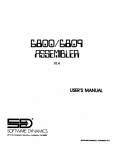
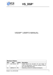
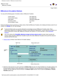
Figure 1 shows a definition in K of untyped λ-calculus with builtin integers, together with a sample
reduction of simple program. Since a more complex language is discussed shortly, we refrain
from commenting this definition here (though the reader may partly anticipate how K works by
trying to decipher it). We only enphasize that the language definition in Figure 1 is formal (it
is an equational theory with initial model semantics) and executable. The five rules on the right
are for initialization of the evaluation process, for collecting and outputing the final result, for
variable lookup, for function evaluation to closures and for function invocation. Any definitional
or implementation framework should explicitly or implicitly provide these operations. From a
language design, semantics and implementation perspective, the fact that one can define λ-calculus
easily in one’s framework should mean close to nothing: any framework worth mentioning should
be capable of doing that. The sole reason for which we depict the definition of λ-calculus here is
to show the reader how a familiar language looks when defined in K. Section ?? shows how K can
modularly define the series of variations of this simple language suggested in [29].
To give the reader a better feel for how K works, we next define an untyped language, that we
call λK , including booleans and integers together with the usual operations on them, λ-expressions
and λ-application, conditionals, references and assignments, and a halt statement. The reader
is encouraged to note the conciseness, clarity and modularity of language feature definitions. To
emphasize the modularity aspect and the strength of context transformers, we then show how one
can extend λK with threads. Appendix D shows a translation of the K definition of sequential λK
below into Maude, while Appendix E shows a translation of its concurrent extension with threads.
Consider the following syntax of non-concurrent λK , where VarList[,] and ExpList[,] stand for
comma separated lists of variables and expressions, respectively:
Var
Bool
Int
Exp
::=
::=
::=
::=
identifier
assumed defined, together with basic bool operations notBool : Bool → Bool, etc.
assumed, together with +Int : Int × Int → Int, <Int : Int × Int → Bool, etc.
Var | Bool | Int | not Exp | Exp + Exp | Exp < Exp | ...
| λVarList[,] .Exp | Exp ExpList[,]
| if Exp then Exp else Exp
| ref Exp | ∗ Exp | Exp := Exp
| halt Exp
Boolean and integer expressions come with standard operations, which are indexed for clarity;
note that we use the infix notation for some of these operations. Expressions of λK extend variables,
booleans, integers, as well as all the “builtin” operations. The λ-abstraction and λ-application are
standard, except that we assume by default that λ-abstractions take any number of arguments.
We deliberately decided not to follow the standard approach in which λ-abstractions are defined
with only one argument and then multiple arguments are eliminated via currying, because that
would change the granularity level of the language definition (see requirement number 6 above);
additionally, most language implementations treat multiple arguments of functions together, as a
block. In our view, from a language definitional and design perspective, a framework imposing such
changes of granularity in a language definition just for the purpose of “reducing every language
feature to a basic set of well-chosen constructs” is rather limited and falls into the same category
with a framework translating any language construct into a sequence of Turing machine operations.
8
Structural operations
k
import INT, K-BASIC
Continuation
State
env
Environment
= VarLocSet
nextLoc
store
LocValSet
Nat
eval : Exp → Val
eval(E) = result(k(E) env(·) store(·) nextLoc(0))
................................
result : State → Val
resultk(V : Val) = V
k(X env(X, L) store(L, V )
Var, Int < Exp
.....................................................
Int < Val
V
+ : Exp × Exp → Exp [!,
+Int : Int × Int → Int]
⎫
⎬
⎧
env(Env)
k(
λ X.E
⎪
⎪
⎪
⎪
⎨ closure(X, E, Env)
λ . : Var × Exp → Exp
: Exp × Exp → Exp [![app]]
.......
⎭
⎪
⎪
k((closure(X, E, Env), V ) app K) env(Env )
closure : Var × Exp × Set[Var Loc] → Val
⎪
⎪
⎩
V bind(X) E Env
Env
Sample reduction (underlined subterms change; other reduction sequences are also possible, but they would all lead to the same result, int(11)):
eval((λx.x + 1)(10))
eval((λx.((x, 1) +))(10))
result(k((λx.((x, 1) +))(10)) env(·) store(·) nextLoc(0))
result(k(((λx.((x, 1) +)), 10) app) env(·) store(·) nextLoc(0))
result(k((λx.((x, 1) +)) (·, 10) app) env(·) store(·) nextLoc(0))
result(k(closure(x, (x, 1) +, ·) (·, 10) app) env(·) store(·) nextLoc(0))
result(k(10 (closure(x, (x, 1) +, ·), ·) app) env(·) store(·) nextLoc(0))
result(k(int(10) (closure(x, (x, 1) +, ·), ·) app) env(·) store(·) nextLoc(0))
result(k((closure(x, (x, 1) +, ·), int(10)) app) env(·) store(·) nextLoc(0))
result(k(int(10) bind(x) (x, 1) + (· : Environment)) env(·) store(·) nextLoc(0))
result(k((x, 1) + (· : Environment)) env((x, loc(0))) store((loc(0), int(10))) nextLoc(1))
result(k(x (·, 1) + (· : Environment)) env((x, loc(0))) store((loc(0), int(10))) nextLoc(1))
result(k(int(10) (·, 1) + (· : Environment)) env((x, loc(0))) store((loc(0), int(10))) nextLoc(1))
result(k(1 (int(10), ·) + (· : Environment)) env((x, loc(0))) store((loc(0), int(10))) nextLoc(1))
result(k(int(1) (int(10), ·) + (· : Environment)) env((x, loc(0))) store((loc(0), int(10))) nextLoc(1))
result(k((int(10), int(1)) + (· : Environment)) env((x, loc(0))) store((loc(0), int(10))) nextLoc(1))
result(k(int(10 +Int 1) (· : Environment)) env((x, loc(0))) store((loc(0), int(10))) nextLoc(1))
result(k(int(11) (· : Environment)) env((x, loc(0))) store((loc(0), int(10))) nextLoc(1))
result(k(int(11)) env(·) store((loc(0), int(10))) nextLoc(1))
int(11)
⇒
⇒
⇒
⇒
⇒
⇒
⇒
⇒
⇒
⇒
⇒
⇒
⇒
⇒
⇒
⇒
⇒
⇒
⇒
Figure 1: K definition of λ-calculus (syntax on the left, semantics on the right) and sample reduction.
9
We will later see that rewriting logic, and implicitly K, allow us to tune the granularity of computation also via equational abstraction: if certain rules are not intended to generate computation
steps in the semantics of a language, then we make them equations; the more equations versus rules
in a language definition, the fewer computational steps (and the larger the equivalence classes of
terms/expressions/programs in the initial model of that language’s definition).
For simplicity, we here assume a call-by-value evaluation strategy in λK ; the other evaluation
strategies for languages defined in K present no difficulty and are taught on a regular basis to
graduate and undergraduate students [24].
NEXT-VERSION: add different parameter passing styles and eventually a LAZY-FUN
. The conditional expression expects its first argument to evaluate to a boolean and then, depending
on its truth value, evaluates to either its second or its third expression argument; note that for
the conditional we used the “mix-fix” syntactic notation, rather then a prefix one. The expression
ref E evaluates E to some value, stores it at some location or reference, and then returns that
reference as a result of its evaluation; therefore, in λK we (semantically) assume that references
are first-class values in the language even though the programmer cannot use them in programs
explicitly, since the syntax of λK does not define references (it actually does not define values,
either). The expression ∗ R, called dereferencing of R, evaluates R to a reference and then returns
the value stored at that reference. The expression R := E, called assignment, first evaluates R to
an (existing) reference r and E to a value v, and then writes v at r; the value v is also the result of
the evaluation of the assignment. Finally, the expression halt E evaluates E to some value v and
then aborts the computation and returns v as a result.
We next define the usual let bindings and sequential composition as syntactic sugar over λK :
• let X = E in E is (λX.E )E,
• let F (X) = E in E is (λF.E )(λX.E),
• let F (X, Y ) = E in E is (λF.E )(λX, Y.E), etc., and
• E; E is (λD.E )E, where D is a fresh “dummy” variable; thus, E is first evaluated (recall
that we assume call-by-value parameter passing), its value bound to D and discarded, and
then E is evaluated.
If these constructs were intended to be part of the language, then these definitions are clearly
not suitable from a computational granularity point of view, because they change the intended
granularity of these language constructs. In Section 6, we show how statements like these and
many others can be defined directly (without translating them to other constructs), in the context
of the more complex FUN language. For now, we can regard them as “notational conventions” for
the more complex, equivalent expressions. With these conventions, the following is a λK expression
that calculates factorial of n (here, n is regarded as a “macro”; also, note that this code cannot be
used as part of a function to return the result of the factorial, because halt terminates the program
— one could do it if one defines parametric exceptions as we do later in the paper, and then throw
an exception instead of halt):
let r = ref n
in let g(m, h) = if m > 1 then (r := (∗r) ∗ m; h(m − 1, h)) else halt (∗r)
in g(n − 1, g)
10
While λK is clearly a very simple toy language, we believe that it contains some canonical
features that any ideal language definitional framework should be able to support naturally. Indeed,
if a framework cannot define λ-expressions naturally than that framework is inappropriate to define
most functional languages and most likely many other non-trivial languages. The conditional
statement has been chosen for two reasons: first, most languages have conditional statements as
a means to allow various control flows in programs, and, second, conditionals have an interesting
evaluation strategy, namely strict in the first argument and lazy in the second and third; therefore,
a naive use of a purely “lazy” or a purely “strict” definitional framework may lead to inconvenient
encodings of conditionals. References are either directly or indirectly part of several mainstream
languages, so they must present no difficulty in any language definitional framework. Finally, halt
is one of the simplest control-intensive language constructs; if a language definitional framework
cannot define halt naturally, then it most likely cannot define any control-intensive statements,
including break and continue of loops, exceptions, and call/cc.
On the other hand, if a language definitional framework can define the λK language above
easily, then it most likely can define many other programming language constructs of interest. Our
purpose for introducing λK here is not to highlight specific features that languages could or should
have, but instead to highlight that a language definitional framework should be flexible enough to
support a rapid, yet formal, investigation of language features, lowering the boundary between new
ideas and executable systems for trying these ideas. An important language feature that we have
deliberately not added yet to λK is concurrency; that is because many existing frameworks were
designed for sequential languages and one may therefore argue that a comparison of those with K
on a concurrent language would not be fair. However, we will add threads to λK shortly and show
how they can be given a semantics in K in a straightforward manner. Concurrent λK shows most
of the subtleties of our framework.
The language definitional framework K consists of two important components:
• The K-notation, which can be regarded as a programming language specific front-end to
rewriting logic, allows users to focus fully on the actual semantics of language features, rather
than on distracting details or artifacts of rewriting logic, such as complete sort and operation
declarations even though these can be trivially inferred from context, or adding conceptually unrelated state context just for the purpose of well formedness of the rewrite logic
theory defining the feature under consideration, even though some partially well formed theory could be completed in a unique way entirely automatically. Besides clarity of definitions
of programming language concepts, an additional driving force underlying the design of the
K-notation was compactness of definitions, which is closely related to modularity of programming language definitions: any unnecessary piece of information (including sort and operation
declarations) that we mention in a language feature definition may work against us when using
that feature in a different context.
• The K-technique is a technique to define programming languages algebraically, based on a
first-order representation of continuations. Recall that a continuation encodes the remaining
computation [23, 26]. Specifically, a continuation is a structure that comes with an implicit
or explicit evaluation mechanism such that, when passed a value (thought of as the value
of some local computation), it “knows” how to finish the entire computation. Since they
provide convenient, explicit representations of computation flows as ordinary data, continuations are useful especially in the context of defining control-intensive statements, such as
11
exceptions. Note, though, that continuations typically encode only the computation steps,
not the store; therefore, one still needs to refer to external data during their evaluation. Traditionally, continuations are encoded as higher-order functions, which is very convenient in
the presence of higher-order languages, because one uses the implicit evaluation mechanism of
these languages to evaluate continuations as well. Our K-technique is, however, not based on
encodings of continuations as higher-order functions. That is partly because our underlying
algebraic infrastructure is not higher-order (though, as we are showing here, one can define
higher-order functions); we can more easily give a different encoding of continuations, namely
one based on lists of tasks, together with an explicit stack-like evaluation mechanism.
We introduce the K-notation and the K-technique together as part of our framework K, because
we think that they fit very well together. However, one can nevertheless use them independently;
for example, one can use the K-notation in algebraic specification or rewrite-based applications
not necessarily related to programming languages, and one can employ the K-technique to define
programming languages in any reduction-based framework, ignoring entirely the proposed notation.
An ideal name for our framework would have been “C”, since our technique is based on continuations
and our trickiest notational convention is that for context transformers, but this letter is already
associated to a programming language. To avoid confusion we use the letter “K” instead.
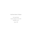
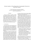
Figure 2 shows the complete definition of λK in K, including both its syntax and its semantics.
The imported modules BOOL, INT and K-BASIC contain basic definitions of booleans, of integer
numbers and of infrastructure operations that tend to be used by most language definitions. We will
discuss these later, together with other technical details underlying the K framework; we here only
mention that these modules can be either defined in the same style as other language features, that
is, as rewrite logic theories using the K framework, or defined or even implemented as builtins. Here
we only present the major characteristics and intuitions underlying the K definitional framework. It
is fair to say upfront that we have not implemented either a parser of K or an automatic translator
of K into rewriting logic or other formalisms yet; currently, we are using it as an alternative to
SOS or reduction semantics to define languages, which can be then straightforwardly translated
into rewrite logic definitions (note that SOS or reduction semantics language definitions cannot
be “straightforwardly” translated into rewriting logic; these need to follow generic and systematic
transformation steps resulting in rather constrained and unnatural rewrite logic theories – see
Section 4). However, K was designed to be implementable as is; therefore, even though we do not
have machine support for it yet, we think of the subsequent definitions, in particular the one of λK
in Figure 2, as machine executable.
The modules BOOL and INT come with sorts Bool, Int and Nat, where Nat is a subsort of Int.
The module K-BASIC comes with sorts Exp, Val and Loc, for expressions, values and locations,
respectively; no subsort relations are assumed among these sorts, in particular the sort Val is not
a subsort of Exp – indeed, values are not expressions in general (e.g., a closure is a value but not
an expression). Locations also come with a constructor operation location : Nat → Loc and an
operation next : Loc → Loc, which gives the next available location; for simplicity, in this paper
we assume that next(location(N )) = location(N + 1), but one is free to define a garbage collector
returning the next unoccupied location. One additional and very important sort that the module
K-BASIC comes with is Continuation, which is a supersort of both Exp and Val (in fact, it is a
supersort of lists of expressions and of lists of values), which is structured as a list (of “tasks”). K
is a modular framework, that is, language features can be added to or dropped from a language
without having to change any other unrelated features. However, for simplicity, we here refrain
12
Structural operations
State
import BOOL, INT, K-BASIC
k
Continuation
eval : Exp → Val
result : State → Val
..........................
env
store
VarLocSet
nextLoc
LocValSet
Nat
⎧
eval(E)
⎪
⎪
⎪
⎪
⎨ result(k(E) env(·) store(·) nextLoc(0))
( 1)
⎪
⎪
⎪
⎪
⎩
( 2)
resultk(V )
V
k(X env(X, L) store(L, V )
Var, Bool, Int < Exp
................................
Bool, Int < Val
V
not : Exp → Exp [!, notBool : Bool → Bool ]
+ : Exp × Exp → Exp [!, +Int : Int × Int → Int]
< : Exp × Exp → Exp [!, <Int : Int × Int → Bool]
⎧
k(
λXl.E
env(Env)
⎫ ⎪
⎪
⎪
closure(Xl, E, Env)
λ . : VarList × Exp → Exp
⎬ ⎪
⎨
: Exp × ExpList → Exp [![app]]
..
⎭ ⎪
⎪
closure : VarList × Exp × VarLocSet → Val
⎪
k((closure(Xl,E,Env),V l) app env(Env )
⎪
⎩
V l bind(Xl) E Env
Env
⎧
bool (true) if(E1 , E2 )
⎪
⎪
⎪
⎪
E1
⎨
if then else : Exp × Exp × Exp → Exp [!(1)[if]]} . . . . . . . . . . . . . . .
⎪
⎪
bool (false) if(E1 , E2 )
⎪
⎪
⎩
E2
⎧
k(V ref nextLoc( L ) store · ⎪
⎪
⎪
⎪
loc(L)
next(L)
(L, V )
⎪
⎪
⎫
⎪
⎪
Loc < Val
⎪
⎪
⎪
⎪
⎨
⎬
k(loc(L) store(L, V )
ref : Exp → Exp [!]
.............
: Exp → Exp [!]
V
⎪
⎪
⎪
⎪
⎭
⎪
⎪
⎪
:= : Exp × Exp → Exp [!]
⎪
⎪
⎪
⎪
k((loc(L), V ) := store(L, )
⎪
⎩
V
V
k(V halt )
..............................................
halt : Exp → Exp [!]
·
Figure 2: Definition of Syntax and Semantics of λK in K
13
( 3)
( 4)
( 5)
( 6)
( 7)
( 8)
( 9)
(10)
(11)
from defining modules and their corresponding module composition operations.
A K language definition contains module imports, declarations of operations (which can be
structural, language constructs, or just ordinary), and declarations of contextual rules. For each
sort Sort, in K we implicitly assume corresponding sorts SortList and SortSet for lists and sets
of sort Sort, respectively. By default, we use the (same) infix associative comma operation ,
as a constructor for lists of any sort, and the infix associative and commutative operation
as a constructor for sets of any sort. One important exception from the comma notation is the
continuation construct, written , which sequentializes evaluation tasks: e.g., the list (E, E ) + write(X) should read “first evaluate the expressions E and E , then sum their values, then
write the result to X”; in module K-BASIC, the sort Continuation is declared as an alias for the sort
ContinuationItemList, where ContinuationItem is declared as a supersort of ExpList and ValList,
and is typically extended with new constructs in a language definition (such as the “+” above).
By convention, tuple sorts Sort1Sort2...Sortn and tuple operations ( , , ..., ) : Sort1 × Sort2 ×
· · · Sortn → Sort1Sort2...Sortn are assumed tacitly, without declaring them explicitly, whenever
needed. Also, some procedure will be assumed for sort inference for variables; this will relieve
us from declaring obvious sorts and thus keep the formal programming language definitions more
interesting and compact. By convention, variables start with a capital letter. If the sort inference
of a variable is ambiguous, or simply for clarity reasons, one can manually sort, or annotate, any
subterm, using the notation t : Sort; in particular, t can be a variable. This manual sorting can be
used by the sort inference procedure to both eliminate ambiguities and improve efficiency.
Structural operations, which we prefer to define graphically as a tree whose nodes are sorts and
whose edges are operation declarations, are those that give the structure of the state. When more
edges go into the same node, the target sort is automatically assumed a multiset sort, each of the
incoming operations generating an element of that set. For example, the sort State in Figure 2
is a set sort, while k (continuation), env (environment), store, and nextLoc (next location) can
generate elements of State; these elements are also called state attributes. All the corresponding set
operation declarations and equations are added automatically. Structural operations will be used
in the process of context transformation of rules that will be explained shortly. The distinguished
characteristic of K is its contextual rule. A contextual rule consists of a term C, called the context,
in which some subterms t1 , ..., tn , which are underlined, are substituted by other terms t1 , ...,
tn , written underneath the lines. Contextual rules can be automatically translated into equations
or rewrite rules. Our motivation for contextual rules came from the observation that in many
rewriting logic definitions of programming languages, large terms tend to appear in the left hand
sides of rewrite rules only to create the context in which a small change should take place; the right
hand sides of such rewrite rules consist mostly of repeating the left ones, thus making them hard
to read and error prone.
When writing K definitions, for clarity we prefer to write the syntax on the left and the corresponding semantics on the right. There will typically be one or at most two semantic rules per
syntactic language construct. At this moment we do not make a distinction between declarations of
operations intended to define the syntax of a language and the declarations of auxiliary operations
that are necessary only to define the semantics; for the time being we assume that the distinction
is clear, but in the forthcoming implementation of K we will have designated operator annotations
for this purpose. Tacitly, we tend to use sans serif font for the former and italic font for the latter.
In the definition of λK in Figure 2, the auxiliary operations eval and result are used to create
the appropriate state context and to extract the resulting value when the computation is finished,
14
respectively. Their definitions consist of trivial contextual rules: eval(E) creates the initial state
with E in the continuation, empty environment and store, and first free location 0, and then
wraps it with the operator result. The rules corresponding to various features of the language will
eventually evaluate E to a value, which will reside as the only item in the continuation at the end
of the computation. Then the rule corresponding to result will collapse everything to that value.
Note the use of the angle brackets “” and “” in the rule for result. These can be used wherever
a list or a set is expected, to signify that there may be more elements to the left or to the right
of the enclosed term, respectively: “t” reads “the term t appears somewhere in the list or set”,
“(t” reads “t appears as a prefix of the list or set”, and “t)” reads “t appears as a suffix of the list
or set”; they are all equivalent in the case of sets, in which case we prefer the former. Intuitively,
“” can be read “and so on to the left” and “” can be read “and so on to the right”. Therefore,
the contextual rule of result says that if the term to reduce will ever consist of a result operator
wrapping a state that contains a continuation that contains a value V , then replace the entire term
by V . The sort Val of V can be automatically inferred, because the result sort of result is Val.
We next say via subsort declarations that variables, booleans and integers are all expressions,
and that booleans and integers are also values. K adds automatically an operation valuesort :
Valuesort → Val for each sort Valuesort that is declared a subsort of Val. In our case, operations
bool : Bool → Val and int : Int → Val are added now, and another operation loc : Loc → Val will be
added later, when the subsort declaration Loc < Val appears. Also, for those sorts Valuesort that
are subsorts of both Val and Exp, a contextual rule of the form
k(
Ev
valuesort(Ev)
is automatically considered in K, saying that whenever an expression Ev of sort Valuesort (inferred
from the fact that Ev appears as an argument of valuesort) appears at the top of the continuation, that is, if it is the next task to evaluate, then simply replace it by the corresponding value,
valuesort(Ev). Rule (3) gives the semantics of variable lookup: if variable X is the next task in
the continuation (note the “” angle bracket matching the rest of the continuation), and if the pair
(X, L) appears in the environment (here note both angle brackets), and if the pair (L, V ) appears
in the store, then just replace X by V at the top of the continuation; note also that the right sorts
for variables can be automatically inferred.
Let us next briefly discuss the operator attributes. The operations not, + , as well as the
other operators extending the builtin operations, have two attributes, an exclamation mark “!”
and the operations they extend. The exclamation mark, called strictness attribute, says that the
operation is strict in its arguments in the order they appear, that is, its arguments are evaluated
first (from left to right) and then the actual operation is applied. An exclamation mark attribute
can take a list of numbers as optional argument and one optional attribute, like in the case of the
conditional. These decorations of the strictness attribute can be fully and automatically translated
into corresponding rules. We next discuss these.
If the exclamation mark attribute has a list of numbers argument, then it means that the
operation is declared strict in those arguments in the given order. Note that the missing argument
of a strictness attribute is just a syntactic sugar convenience; indeed, an operator with n arguments
which is declared just “strict” using a plain “!” attribute, is entirely equivalent to one whose
attribute is “!(1 2 . . . n)”. When evaluating an operation declared using a strictness attribute,
the arguments in which the operation was declared strict (i.e., the argument list of “!”) are first
15
scheduled for evaluation; the remaining arguments need to be “frozen” until the other arguments
are evaluated. If the exclamation mark attribute has an attribute, say att, then att will be used as
a continuation item constructor to “wrap” the frozen arguments. Similarly, the lack of an attribute
associated to a strictness attribute corresponds to a default attribute, which by convention has
the same name as the corresponding operation; to avoid confusion with underscore variables, we
drop all the underscores from the original language construct name when calculating the default
name of the attribute of “!”. For example, an operation declared “ + : Exp × Exp → Exp [!]” is
automatically desugared into “ + : Exp × Exp → Exp [!(1 2)[+]]”.
Let us next discuss how K generates corresponding rules from strictness attributes. Suppose
that we declare a strict operation, say op, whose strictness attribute has an attribute att. Then K
automatically adds
(a) an auxiliary operation att to the signature, whose arguments (number, order and sorts) are
precisely the arguments of op in which op is not strict; the result sort of this auxiliary
operation is ContinuationItem;
(b) a rule initiating the evaluation of the strict arguments in the specified order, followed by the
other arguments “frozen”, i.e., wrapped, by the corresponding auxiliary operation att.
For example, in the case of λK ’s conditional whose strictness attribute is “!(1)[if]”, an operation
“if : Exp × Exp → ContinuationItem is automatically added to the signature, together with a rule
if E then E1 else E2
E if(E1 , E2 )
If the original operation is strict in all its arguments, like not, + and , then the auxiliary
operation added has no arguments (it is a constant). For example, in the case of λK ’s application
whose strictness attribute is “![app]”, an operation “app : → ContinuationItem is added to the
signature, together with a rule
E El
(E, El) app
The “builtin” operations added as attributes to some language constructs, such as +Int : Int×
Int → Int as an attribute of + : Exp × Exp → Exp, each corresponds to precisely one K-rule
that “calls” the builtin on the right arguments. This convention will be explained in detail later in
the paper; we here only show the two implicit rules corresponding to the attributes of the addition
operator in Figure 2:
E1 + E2
(E1 , E2 ) +
(int(I1 ), int(I2 )) +
int(I1 +Int I2 )
Notice that these rules can apply anywhere they match, not only at the top of the continuation. In
fact, the rules with exclamation mark attributes can be regarded as some sort of “precompilation
rules” that transform the program into a tree (because continuations can be embedded) that is
more suitable for the other semantic rules. If, in a particular language definition, code is not
generated dynamically, then these pre-compilation rules can be applied all “statically”, that is,
16
before the semantic rules on the right apply; one can formally prove that, in such a case, these
“pre-compilation” rules need not be applied anymore during the evaluation of the program. These
rules associated to exclamation mark attributes should not be regarded as transition rules that
“evolve” a program, but instead, as a means to put the program into a more convenient but
computationally equivalent form; indeed, when translated into rewriting logic, the precompilation
contextual rules become all equations, so the original program and the precompiled one are in the
same equivalence class, that is, they are the same program within the initial model semantics that
rewriting logic comes with.
To get a better feel for how the rules corresponding to strictness attributes change the syntax of
a program, let us consider the λ-expression corresponding to the definition body of the g function
in our definition of factorial in λK above, namely
if m > 1 then (r := (∗r) ∗ m; h(m − 1, h)) else halt (∗r).
The strictness rules associated automatically to the exclamation mark attributes transform this
term in a few steps (that can also be applied in parallel on a parallel rewrite engine) into
(m, 1) > if((λd . (r, (r ∗, m) ∗) :=)((h, (m, 1) −, h) app), r ∗ halt).
We have also applied the notational convention for sequential composition and assumed that the
continuation constructor binds the tightest. Therefore, these “precompilation” rules (that
can be generated automatically from the exclamation mark attributes of operators) do nothing but
iteratively transform the expression to evaluate in a postfix form, taking into account the strictness
information of language constructs. Since we’ll refer to this expression several times in Figure 3,
we introduce the “macro” %G to refer to it.
Let us discuss the remaining contextual rules in Figure 2. Rule (4) says that a λ-abstraction
evaluates to a closure. The current environment is needed, so it is mentioned as part of the rule.
Note that a closure is a value but not an expression. Rule (5) gives the semantics of application
(defined as a strict operation): it expects to be passed a closure and a value V ; it then binds the
list of values Vl to the list of parameters Xl in the closure in the environment Env of the closure,
which becomes current, and then initiates the evaluation of E, the body of the closure; the original
environment Env’ is recovered after the resulting value is produced. The semantics of bind(Xl) and
environment recovery are straightforward and assumed part of the module K-BASIC, since they
are used in most languages that we defined; they will be formally defined and discussed in detail
in Section 5.
Rules (6) and (7) give the expected semantics of the conditional statement. Recall that the
conditional is declared strict in its first argument, so an auxiliary operation if is generated together
with the rule above initiating the evaluation of the condition. Rules (8), (9) and (10) give the
semantics of references, one per corresponding language construct. Note first that Loc is defined
as a subsort of Val, so an operation loc : Loc → Val is implicitly assumed. Note also that all the
language constructs for references are strict, so we only need to define how to combine the values
produced by their arguments. Rule (8) applies when a value is passed to the auxiliary operator ref
at the top of the continuation; when that happens, a corresponding location value is produced, the
current next location is incremented, and the value is stored at the newly produced location in the
store. Note the use of angle brackets to match the unit “·” of the store multiset. By convention,
in K we use the dot “·” as the unit of all set and list structures. In this case, matching the unit
somewhere in the store always succeeds, and replacing it by a pair corresponds to adding that
17
pair to the store. Rule (9) for dereferencing location L grabs the value V at location L in the
store, and rule (10) for assignment replaces the exiting value at location L in the store by V ;
underscore variables can be used any time when the corresponding matched term is not needed
for any other purpose (except the actual matching) in the rule - in other words, variables that
appear only once in a rule can well be underscores. Finally, rule (11) for halt simply dissolves the
rest of the continuation, keeping only the value on which the program halted. If the evaluation of
the argument expression E of halt(E) encounters another halt, then the nested halt will obviously
terminate the execution of the program (the outer halt that initiated the evaluation of E will be
dissolved as a consequence of applying the rule (11) for the nested halt).
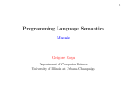
Figure 3 shows the “execution”1 of λK (as defined in K) on the factorial program above, where
n is 3. Each line shows a term. The underlined subterms of each term are those that change by the
application of contextual rules. The rules applied are mentioned on the right column, above the
arrow ⇒: !∗ means a series of application of implicit rules associated to ! attributes; (4), for example,
means an application of the contextual rule (4); [K] stays for basic rules that come with the module
K-BASIC. If one collapses all the applications of non-numbered contextual rules (which is precisely
what happens semantically anyway, because all these contextual rules are translated into equations
in the associated rewrite logic theory), then one can see exactly all the intended computation steps
of this execution (making abstraction, of course, of their syntactic representation). Despite its
computational feel, the “execution” in Figure 3 is actually a formal derivation, or proof, that the
factorial of 3 indeed reduces to 6 within the formal semantics of our programming language. It is,
however, entirely executable; in fact, the derivation in Figure 3 was produced by tracing Maude’s
reduction (with the command “set trace on .”) of the factorial program within the Maude-ified
version of the K semantics in Figure 2; this Maude semantics is shown in Appendix D.
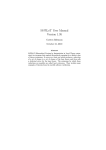
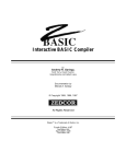
Let us next add concurrency to λK ; we do it by means of dynamic threads. To keep the
language simple, we refrain from adding any built-in synchronization mechanism here. We will add
synchronization via acquire and release of locks later in the paper, in the context of defining the
more complex language FUN; for now, one can partially simulate synchronization by programming
techniques (using wait-loops and shared variables). Our point here is to emphasize that adding
threads to λK is a straightforward task, requiring no change of the already defined language features.
The additional work needed is shown in Figure 4 and it is, in our view, conceptually unavoidable
unless one makes stronger assumptions about the possible extensions of the language apriori; for
example, if one assumes that any language can be potentially extended with threads, then one can
define for non-concurrent λK the state as in Figure 4 from the very beginning (rather than as in
Figure 2). However, this would not be a general solution, because one cannot know in advance
how a language will be extended; for example, how can one know that λK is not going to be
extended with concurrency using actors [1] instead of threads? (In fact, this is in our opinion
quite an appealing extension.) A major factor in the design of K, whose importance increasingly
became clear to us empirically by experience with several language definition case studies, was the
observation that whenever one extends an existing language by adding new features, or whenever
one builds a language by combining features already defined in some library, one cannot and does
not want to avoid analyzing and deciding on “the structural big picture” of the language, namely
how the state items needed by the various desired language features are structured within the state
of the language (recall that our notion of “state” is broad and generic).
We want the threads in λK to be dynamically created and terminated. Like in any multi1
We warmly thank Traian Florin Şerbănuţa for help with typing in this sample execution.
18
eval((λr . (λg . g(3 − 1, g))(λm, h . if m > 1 then (λd.h(m − 1, h) (r := (∗r) ∗ m)) else halt (∗r))) (ref 3))
eval(((λr . ((λg . (g, (3, 1) −, g) app), λm, h .%G) app), 3 ref) app)
result(k(((λr . ((λg . (g, (3, 1) −, g) app), λm, h . %G) app), 3 ref) app) store(.) nextLoc(0) env(.))
result(k((λr . ((λg . (g, (3, 1) −, g) app), λm, h . %G) app) (3 ref, ·) app) store(.) nextLoc(0) env(.))
result(k(closure(r, ((λg . (g, (3, 1) −, g) app), λm, h . %G) app, ·) (3 ref, ·) app) store(.) nextLoc(0) env(.))
result(k(3 ref (·, closure(r, ((λg . (g, (3, 1) −, g) app), λm, h . %G) app, ·)) app) store(.) nextLoc(0) env(.))
result(k(loc(0) (·, closure(r, ((λg.(g, (3, 1) −, g) app), λm, h.%G) app, ·)) app) store((0, 3)) nextLoc(1) env(.))
result(k((closure(r, ((λg.(g, (3, 1) −, g) app), λm, h.%G) app, ·), loc(0)) app) store((0, 3) ·) nextLoc(1) env(.))
result(k((λg.(g, ((3, 1) −), g) app) (λm, h.%G, .) app (.)) store((0, 3)(1, loc(0))) nextLoc(2) env((r, 1)))
!∗
⇒
(1)
⇒
[K]
⇒
(4)
⇒
[K]
⇒
(8),[K]
⇒
[K]
⇒
(5),[K]
⇒
(4),[K]
⇒
result(k((closure(g, (g, ((3, 1) −), g) app, (r, 1)), %C1) app (.)) store((0, 3)(1, loc(0)) ·) nextLoc(2) env((r, 1)))
(5),[K]
result(k(g (((3, 1) −), g, .) app ((r, 1)) (.)) store((0, 3)(1, loc(0))(2, %C1)) nextLoc(3) env((g, 2)(r, 1)))
(3),[K]
result(k((%C1, 2, %C1) app ((r, 1)) (.)) store((0, 3)(1, loc(0))(2, %C1) ·) nextLoc(3) env((g, 2)(r, 1)))
(5),[K]
result(k(m (1, .) > %IF ((g, 2)(r, 1)) ((r, 1)) (.)) %S1)
(3),[K]
result(k(bool(true) %IF %e1) %S1)
(6),[K]
⇒
⇒
⇒
⇒
⇒
result(k((λd.(h, ((m, 1) −), h) app) ((r, ((r ∗), m) ∗) :=, .) app %e1) %S1)
(4,3),[K]
⇒
result(k(loc(0) ∗ (m, .) ∗ (., loc(0)) := (., %C2) app %e1) %S1)
(9),[K]
result(k(m (., 3) ∗ (., loc(0)) := (., %C2) app %e1) %S1)
(3),[K]
result(k((loc(0), 6) := (., %C2) app %e1) store((0, 3) %s1 ) nextLoc(5) env((h, 4)(m, 3)(r, 1)))
⇒
⇒
(10),[K]
⇒
result(k((%C2, 6) app %e1) store((0, 6) %s1 ·) nextLoc(5) env((h, 4)(m, 3)(r, 1)))
(5),[K]
result(k(h (((m, 1) −), h, .) app %e2) store((0, 6) %s1 (5, 6)) nextLoc(6) env((d, 5)(h, 4)(m, 3)(r, 1)))
(3),[K]
result(k((%C1, 1, %C1) app %e2) store((0, 6) %s1 (5, 6) ·) nextLoc(6) env((d, 5)(h, 4)(m, 3)(r, 1)))
(5),[K]
result(k(m (1, .) > %IF %e3) %S2)
(3),[K]
⇒
⇒
⇒
⇒
(7)
result(k(bool(f alse) %IF %e3) %S2)
⇒
(3)
result(k(r ∗ halt %e3) %S2)
⇒
(9)
result(k(loc(0) ∗ halt %e3) %S2)
⇒
(11)
result(k(6 halt %e3) %S2)
⇒
(2)
⇒
result(k(6) %S2)
6
%IF stands for if((λd.(r, (r ∗, m) ∗) :=)((h, (m, 1) −, h) app), r ∗ halt)
%G stands for (m, 1) > %IF
%C1 stands for closure(m, h, %G, (r, 1))
%S1 stands for store((0, 3) %s1 ) nextLoc(5) env((h, 4)(m, 3)(r, 1)))
%e1 stands for ((g, 2)(r, 1)) ((r, 1)) (.)
%C2 stands for closure(d, (h, ((m, 1) −), h) app, (h, 4)(m, 3)(r, 1))
%s1 stands for (1, loc(0))(2, %C1)(3, 2)(4, %C1)
%e2 stands for ((h, 4)(m, 3)(r, 1)) %e1
%e3 stands for ((d, 5)(h, 4)(m, 3)(r, 1)) %e2
%S2 stands for store((0, 6) %s1 (5, 6)(6, 1)(7, %C1)) nextLoc(8) env((h, 7)(m, 6)(r, 1))
Figure 3: Sample run of the factorial program in the executable semantics of λK in K.
19
Structural operations
The definition of λK in Figure 2
needs to be changed as follows:
1) replace structural operators with
the ones in the picture to the right
2) replace definition of eval as below
3) add two more rules, as below:
a) one for creation of threads; and
b) one for termination of threads
No other changes needed.
State
thread
*
ThreadState
k
Continuation
nextLoc
store
LocValSet
Nat
env
Env
eval(E)
result(thread(k(E) env(·)) store(·) nextLoc(0))
spawn : Exp → Exp
die : · → ContinuationItem
( 1)
⎧
·
(12)
⎪
⎪ thread(k(spawn E env(Env))
⎪
⎪
0
thread(k(E die) env(Env))
⎨
⎪
⎪
⎪
⎪
⎩
threadk(V : Val die) (13)
·
Figure 4: Adding threads to λK
threaded language, threads in λK may share memory locations. More precisely, a newly created
thread shares the same environment as its parent thread. Therefore, accesses (reads or writes)
to variables shared by different threads may lead to non-deterministic behaviors of programs (in
particular to data-races). All these suggest to the language designer the state structure depicted
in Figure 4 for multi-threaded λK . Its state therefore contains, besides a store and a next available
location like in the non-concurrent version, an arbitrary number of threads. The star () on the
arrow labeled thread in the graph in Figure 4 means that corresponding subterms wrapped by the
state constructor operator thread can appear multiple times in the state — in this case, reflecting
the fact that the number of threads created during the execution of a program varies. The star
annotation happens to be irrelevant in the definition of multi-threaded λK , but in other language
definitions it may play a critical role in the disambiguation of the context transformation process
discussed next. Each subterm in the state soup wrapped by a thread construct (i.e., each thread)
contains a continuation k(...) and an environment env(...).
The next step is to create the initial state of a program. Unlike in non-concurrent λK where
the initial state contained the continuation and the environment at the same top level as the store
and the next available location, in multi-threaded λK the initial state should contain one thread at
the same top level as the store and the next available location, but the continuation associated to
the program to evaluate as well as its corresponding (empty) environment should be contained as
part of that thread, rather than at the top level (so we have a “nested soup”). This way, several
threads with their corresponding continuations and environments can be unambiguously created,
20
terminated and accessed dynamically. The semantics of the operation eval needs to be changed
now to appropriately initiate the evaluation of its argument expression taking into consideration
the new initial state.
An intriguing observation at this stage is that many of the contextual rules in Figure 2 do not
parse anymore because of the new state structure, and so does the sample execution in Figure 3.
Therefore, it looks as if the addition of threads to λK broke the modularity of the other language
feature definitions. That would be, indeed, the case in the context of most language definitional
frameworks, including SOS as well as plain rewrite logic definitions of languages. However, in K
we need to change no existing definitions of other language features, even though they were defined
before the state structure of multithreaded λK was known. That is thanks to one of the most
important features of K, called context transformer and explained next.
In K, the structural operators play a crucial role in the definition of a language. Many of
the contextual rules in a K definition of a language are incomplete unless full knowledge of the
state structure is available. That incompleteness allows language designers to only mention the
relevant part of the state when defining the semantics of each feature. An advantage of rewrite
logic definitions compared to SOS definitions is that in a rewrite rule one needs only mention
the local structure of a subterm on which a transformation is applied, while in traditional SOS
definitions one needs to mention the entire state, or configuration, even though one wants to change
only a very small portion of it. Thanks also to matching modulo associativity, commutativity and
identity which bring additional modularity to language definitions, rewriting logic allows for elegant
and compact definitions even of complex features of languages [19, 18]. However, rewriting logic
imposes well-formedness of its rewrite rules w.r.t. signatures, so definitions of features cannot be
easily transported from one language to another when the structure of the state changes. K’s
context transformers address precisely this limitation of rewriting logic. At this moment we solve
all the context transformers statically because we assume that the structure of the state does not
change. However, one could also imagine, at least in principle, more complex situations in which
the structure of the state would change dynamically; in such a case one could informally think of
context transformers as of matching modulo structure.
Context transformers will be explained in detail later in the paper; we here only discuss their
application on multi-threaded λK . Intuitively, once all the structural operators are known, such
as in the pictures in Figures 2 and 4, the contextual rules need not mention the complete “path”
to each operation that appears in a rule, because that path can be inferred automatically and
unambiguously from the declared structure of the state. For example, consider rule (2) in Figure 2
defined for non-concurrent λK , but when the structure of the language changes as in Figure 4. This
rule obviously does not parse anymore, because result expects an argument of sort State which,
because of the structural operators in Figure 4, can only be constructed with state constructors
thread(...), store(...), and nextLoc(...); therefore, there is no k(...) construct at the top level of
the state anymore, so resultk(V ) naturally does not parse. However, the crucial observation
is that there is a unique way to have k(V ) make sense in a term below the operation result:
when k(V ) is part of a thread state, wrapped by the operator thread. Therefore, by taking the
structural operators into account, one can automatically and unambiguously transform resultk(V )
into resultthreadk(V ), the latter making now full sense in the new language definition. Similarly,
with the new state structure in Figure 4, one can automatically transform rule (3) in Figure 2 into
21
threadk(X env(X, L) store(L, V ).
V
Since a thread has only two soup attributes each with multiplicity one, namely a continuation
and an environment, the angle brackets of thread could have been just plain parentheses. There
are guidelines that need to be followed and conventions that need to be adopted in order for the
context transformation process of rules to be unambiguous; these are discussed in more depth in
Section 5.9. As a rule of thumb, terms that appear in a contextual rule are grouped in a “depthfirst” style. For example, in the rule (3) for variable lookup above, we grouped the continuation
and the environment together and placed them inside one thread; one could have also put each of
the two in one separate thread, but that would have violated the “depth first” style. However, if
two continuations were involved in some contextual rule (that is indeed possible in some language
definitions), then that rule would be transformed into one where each continuation appears in
its separate thread; that’s because the structural operations picture in Figure 4 specifically allows
threads, not continuations, to appear multiple times in the state (the star “” on the arrow thread).
All contextual rules defining the sequential features of λK in Figure 2 can be automatically
transformed in a similar manner when transported into the definition of multithreaded λK . Let us
next discuss the concurrent features of multithreaded λK . Spawning a new thread to calculate an
expression E can be done from any other thread. The contextual rule (12) shows the semantics of
spawn(E): a new thread is added to the state soup that contains the expression to evaluate E in its
continuation and shares the same environment as the creating thread; spawn(E) evaluates to 0 (by
convention; like in FUN defined later in the paper, we could have also added a special “unit” value
and evaluate all constructs used for their side effects to that particular value) with no delay, and
a die continuation item is placed after the expression E in the created thread to state that that
thread should be terminated (and therefore removed from the state) once E evaluates to a value
(this is done by rule (13)). In a more complex language, such as FUN, the resources of a thread
(e.g., the locks it holds) need to be released as well when the thread is terminated.
An interesting observation here, which has nothing to do with K as a definitional framework
but only with our particular design of multi-threaded λK , is that any thread can halt the program.
Indeed, the rule for halt can be applied for any thread and, if applied on a created thread, the
terminating continuation item die is eliminated and therefore rule (2) for returning the result can
apply, thus returning the halted value as a result of the entire multi-threaded program. Note
that the only way that rule (2) can apply on the continuation of a spawned thread is that that
thread halts the computation; otherwise, the continuation item die would follow the value in the
continuation, so rule (2) would be inapplicable. Since rules can be applied non-deterministically
(and they would indeed be applied non-deterministically on a parallel rewrite engine), there is no
guarantee that all the threads will be properly terminated before the final result is produced, even
if no thread halts the computation. For example, the original thread may spawn a thread as the
last task in its computation; this spawning will produce a 0 in the continuation of the original
thread and, as a side effect, will create the new thread; now rule (2) can apply on the continuation
of the original thread without waiting for the created thread to terminate.
The K framework will be discussed more fully in Sections 5 and 6, where we also define FUN,
a more complex programming language with higher-order functions with return, let and letrec,
lists, sequential composition, assignments, loops with break and continue, input/output, parametric
exceptions, call/cc and concurrency via threads and synchronization. In this introduction we only
22
wanted to emphasize that once learned, K is simple, natural, and leads to compact and easy to
understand and read language definitions. An interesting feature of K that we have not discussed
so far but which is also worthwhile mentioning, is the distinction that it makes among contextual
rules. These can be:
• Structural, or non-computational. These are rules whose only role is to allow modifications of
the structure of the state, so that other contextual rules that have computational meaning can
apply. For example, the rules generated automatically by K for the strictness attributes (“!”)
as well as rule (1) are all structural, their role being to prepare the expression for evaluation
by prioritizing the subexpressions that need to be evaluated first. Also, all the set and list
implicit associativity and commutativity equations are structural, having no computational
meaning.
• Computational. These are rules that each captures precisely one intended execution step of
the program. All numbered rules in the definition of λK except (1) are computational.
• Non-deterministic. These are rules that can potentially change the deterministic behavior of
a program. If a language is sequential and deterministic, then there is no need to declare any
contextual rule to be non-deterministic, because the rules are expected to be Church-Rosser
on the terms of interest (well-formed programs). However, if a language admits concurrency,
then some rules may lead to non-deterministic executions; for example, reads and writes of
memory locations, or acquires of locks.
Non-deterministic rules are always a (typically quite small) subset of the computational rules.
The structural and computational declarations of contextual rules are modular, in the sense that
one does not need knowledge about the entire language in order to declare a rule structural or
computational. However, the non-deterministic declaration of rules is trickier and needs global
information about the program. For example, one cannot know when one defines a variable lookup
rule (3) whether the defined language is concurrent or not; if it is, then that rule needs to be declared
non-deterministic. Also, it is impossible to identify the non-deterministic rules automatically in
general (this problem is harder than testing confluence).
K can be all resolved statically, so a definition of a language in K is a rewrite logic specification.
One subtle aspect of the translation of K into rewriting logic is to decide which contextual rules
translate into equations and which into rewrite rules (see Section 3 for the semantic distinction
between the two). In general, if one is interested in obtaining just one interpreter or a dynamic semantics for the language, then one can translate all the computational contextual rules into rewrite
rules and the non-computational ones into equations. If formal analysis of programs is of interest,
then one may want to reduce the number of rewrite rules to a minimum; this can be done by
transforming only the non-deterministic contextual rules into rewrite rules. Since rewriting logic
is efficiently executable (rewrite engines such as ASF+SDF and Maude are quite fast), relatively
efficient interpreters are obtained for free from such formal language definitions. However, K specifications follow a certain definitional methodology which identifies them as particular rewrite logic
specifications. Therefore, one should be able to execute these K definitions more efficiently using
some specialized rewrite engines or compilers than using general purpose rewrite engines such as
ASF+SDF or Maude. Some preliminary experiments have been made showing that that is indeed
the case; Section 11 gives more details.
Also, formal analysis tools for rewrite logic specifications, such as those of Maude [5] (e.g., model
checkers), translate into corresponding tools for languages defined using the presented technique.
23
Also, since rewriting logic is a computational logical framework with both initial model semantics
and formal analysis techniques for initial models, the presented framework can also serve as a
foundation for program verification. The technique presented here, or previous versions of it, has
been used to define language features including type inference, object-orientation and subtyping,
concurrency, etc., as well as large fragments of real programming languages, such as the λ-calculus,
System F, Beta, Haskell, Java, LLVM, LISP, Python, Pict, Ruby, and Smalltalk [24].
As discussed in [7] and Section 10, the model checker obtained for free from the formal definition
of Java compares favorably with two state of the art Java model checkers.
24
3
Rewriting Logic
The language definitional framework proposed in this paper can be presented and understood
in isolation, like SOS or reduction semantics, and implemented following different programming
paradigms. However, as mentioned previously, we prefer to present it via an automatic translation
to term rewriting modulo equations or to rewriting logic, for two reasons:
1. to make it clear upfront that we inherit all the good properties of these well understood and
generic computational frameworks, and
2. to use at no additional effort the remarkable rewrite-based tool support developed over the
last few decades.
We here informally recall some basic notions of rewriting logic and of its important sublogic called
equational logic, together with operational intuitions of term rewriting modulo equations.
3.1
Equational Logics
Equational logic is perhaps the simplest logic having the full expressivity of computability [2].
One can think of it as a logic of “term replacement”: terms can be replaced by equal terms in
any context. An equational specification is a pair (Σ, E), where Σ is a set of “uninterpreted”
operations, also called its “syntax”, and E is a set of equations of the form (∀X) t = t constraining
the syntax, where X is some set of variables and t, t are well-formed terms over variables in X
and operations in Σ. Equational logics can be many-sorted [10] (operations in Σ have arguments
of specific sorts), or even order-sorted [11], i.e., sorts come with a partial order on them; we use
order-sorted specifications in this paper. Also, equations can be conditional, where the condition
is a (typically finite) set of pairs u = u over the same variables X. We write conditional equations
(of finite condition) using the notation (∀X) t = t ⇐ u1 = u1 ∧ · · · ∧ un = un .
Models of an equational specification (Σ, E) interpret sorts into sets of values and operations in
Σ into corresponding functions satisfying all the equations in E, where a model satisfies an equation
if and only if the two terms evaluate to the same value for any assignment of their variables to
values in the model. Models are also called Σ-algebras and it is customary to regard them as
“realizations”, or even “implementations”, of the equational specifications they satisfy. Equational
deduction is complete and consists of five natural deduction rules, namely reflexivity, symmetry,
transitivity, congruence and substitution. We write E Σ e if the equation e can be derived with
these rules from (Σ, E). Among the variety of models of an equational specification, there is one
which, up-to-an-isomorphism, captures precisely the intended meaning of the specification: its
initial model. Because of the “all-in-one and one-in-all” flavor and properties of initial algebras,
as well as because any computable domain can be shown isomorphic to a (restricted) initial model
over a finite equational specification [2], initial algebra semantics [12] was introduced in 1977 as a
theoretically self-contained approach to (non-concurrent) programming language semantics.
3.2
Term Rewriting
Term rewriting is a related approach in which equations are oriented left-to-right, written (∀X) l →
r and called rewrite rules, and can be applied to a term t at any position where l matches as follows:
find some subterm t of t, that is, t = c[t ] for some context c, which is an instance of the left-handside term (lhs) of some rewrite rule (∀X) l → r, that is, t = θ(l) for some variable assignment θ,
25
and replace t by θ(r) in t. This way, the term t can be continuously transformed, or rewritten.
A pair (Σ, R), where R is a set of such oriented rewrite rules, is called a rewrite system. The
corresponding term rewriting relation is written →R and its inverse is written ←R . If no rule in R
can rewrite a Σ-term, than that term is said to be in normal form w.r.t. R.
Term rewriting can be used as an operational mechanism to perform equational deduction.
Specifically, E Σ (∀X) t = t if and only if t (→RE ∪ ←RE )∗ t , where RE is the set of rewrite
rules obtained by orienting all the equations in E from left to right. Therefore, term rewriting is
as powerful as equational deduction if used in both directions. However, in practice term rewriting
is used as a heuristic for equational deduction. A very common case is to attempt the task E Σ
(∀X) t = t by showing t →∗RE · ←∗RE t , i.e., by reducing both t and t to some common term
using (Σ, RE ). In some cases, for example when (Σ, RE ) is confluent and terminates, this becomes
a semi-decision procedure for equational deduction.
There are many software systems that either specifically implement term rewriting efficiently,
known also as rewrite engines, or that support term rewriting as part of a more complex functionality. Any of these systems can be used as an underlying platform for execution and analysis
of programming languages defined using the technique and the formalism proposed in this paper.
Without attempting to be exhaustive, we here only mention (alphabetically) some engines that
we are more familiar with, noting that many functional languages and theorem provers provide
support for term rewriting as well: ASF/SDF [27], CafeOBJ [6], Elan [3], Maude [5], OBJ [13],
Stratego [28]. Some of these can achieve remarkable speeds on today’s machines, in the order of
millions or tens of millions of rewrite steps per second. Many engines store terms as directed acyclic
graphs (DAGs), so applications of rewrite rules consist in many cases of just permuting pointers,
which can indeed be implemented quite efficiently. In our language definitions, we often place or
remove environments or continuations onto other structures; even though these may look like heavy
operations, in fact these do nothing but save or remove pointers to subterms when these definitions
are executed.
Because of the forward chaining executability of term rewriting and also because of these efficient
rewrite engines, equational specifications are often called executable. As programming languages
tend to be increasingly more abstract due to the higher speeds of processors, and as specification
languages tend to be provided with faster execution engines, the gap between executable specifications and implementations, in case there has ever been any, is becoming visibly narrower. For
example, we encourage the curious reader to specify the factorial operation equationally as follows
(s is the Peano “successor”)
0! = 1
s(N )! = s(N ) ∗ N !
in a fast rewrite engine like Maude, versus implementing it in programming languages like ML or
Scheme. In our experiments, the factorial of 50,000, a number of 213,237 digits, was calculated in
18.620 seconds by the executable equational engine Maude and in 19.280 and 16.770 seconds by
the programming languages ML and Scheme, respectively. In case one thinks that the efficiency
of builtin libraries should not be a factor in measuring the efficiency of a system, one can define
permutations equationally instead, for example as follows
Sorts and Subsorts
Nat < Permutation < Permutations
Operations
, : Permutation Permutation → Permutation [assoc]
26
; : Permutations Permutations → Permutations [assoc]
perm : Nat → Permutations
insert : Nat Permutations → Permutations
map-cons : Nat Permutations → Permutations
Equations
perm(1) = 1
perm(s(N )) = insert(s(N ), perm(N ))
insert(N , (P :Permutation ; Ps:Permutations)) = insert(N ,P ) ; insert(N ,Ps)
insert(N, (M,P’)) = (N,M,P’) ; map-cons(M, insert(N,P’))
insert(N, M) = (N,M) ; (M,N)
map-cons(M, (P ; Ps)) = map-cons(M, P) ; map-cons(M, Ps)
map-cons(M, P) = (M,P)
The above is an order-sorted equational specification; for readability, we used the mixfix notation for
operation declarations (underscores are argument placeholders) which is supported by many rewrite
engines. Also, we declared the list constructor operations with the attribute [assoc]. Semantically
this is equivalent to giving the equation of associativity, but rewrite engines typically use this
information to enable specialized algorithms for rewriting and matching modulo associativity; we
will discuss matching modulo attributes like associativity, commutativity and identity in more
depth shortly. Like in the previous example, we assumed some builtin natural numbers coming
with a successor operation.
In our experiments with permutations, the executable equational specifications outperformed
the implementations. Maude took 61 seconds to “calculate” permutations of 10, while ML and
Scheme took 83 and 92 seconds, respectively. None of these systems were able to calculate permutations of 11. These experiments have been performed on a 2.5GHz Linux machine with 3.5GB
of memory, and we2 used Maude 2.0, PolyML and PLT Scheme (specifically mzscheme), all providing libraries for large numbers. These simplistic experiments should by no means be considered
conclusive; our measurements favoring executable specifications may be due to fortunate uses of
data-structures in the Maude implementation, or even to our lack of usage of Scheme and ML at
their maximum efficiency. While more extensive comparisons and analyses would be interesting
and instructive, this is not our goal here; nor to unreasonably claim that executable specifications
will ever outperform implementations. All we are trying to say is that the pragmatic, semanticsreluctant language designer, can safely regard the subsequent semantic definitions of language
features as implementations, in spite of their conciseness and mathematical flavor.
NEXT-VERSION: discuss the examples with white/black balls and with bubble sorting
3.3
Rewriting Logic
While equational logic and its execution via term rewriting provide as powerful computational
properties as one can get in a sequential setting, these were not designed to specify or reason
about concurrent systems. The initial algebra model of an equational specification collapses all
the computationally equivalent terms, but it does not say anything about evolution of terms under
concurrent transitions. There are at least two broad directions of research on the subject of specifying non-deterministic and/or concurrent systems [30]. One builds upon the Platonist belief that
2
Warmest thanks to Mark Hills who helped with these experiments.
27
models are deterministic, but, by making use of underspecification, one never knows precisely in
which model one is3 . While underspecification is a very powerful approach in semantics, in our programming language definitional framework it suffers from a crucial impediment: it is not executable
enough to allow one to execute actual concurrent programs. Nevertheless, we will make intensive
use of underspecification by not specifying implementation details of programming languages (such
as how environments, stores, lists or stacks are implemented). Another direction of thought in
concurrency is to allow non-determinism in models, typically by means of non-deterministic transitions. Specifications become executable now, because all what one needs to do is to randomly
pick some transition when more are possible. This is similar to what thread/process schedulers do
in concurrent computer systems.
To properly define and analyze (concurrent) programming languages formally, we need a framework which provides natural support for concurrency. In other words, we would like a framework
in which we can state what programming language features are meant to do without artificial encodings of these due to artifacts of the underlying definitional framework. For example, we would
consider it “unnatural” to define, or simulate, a particular “thread or process scheduler” in order
to define a concurrent language, just because the underlying definitional framework is inherently
sequential. Since both underspecification and non-deterministic transitions seem important for
capturing the meaning of programming language features, we would like an underlying framework
that supports both.
Rewriting logic [17] is a logic for concurrency, which should not be confused with term rewriting.
A rewrite specification, or theory, is a triple (Σ, E, R), where (Σ, E) is an equational specification
and R is a set of rewrite rules. Rewriting logic therefore extends equational logic with rewrite rules,
allowing one to derive both equations and rewrites (or transitions). Deduction remains the same
for equations, but the symmetry rule is dropped for rewrite rules. Models of rewrite theories are
(Σ, E)-algebras enriched with transitions satisfying all the rewrite rules in R. In our context, the
equational part of a rewrite theory is allowed to “underspecify” features as far as the specification
remains executable. Interestingly, rewrite theories also have initial models, consisting of term
models factored by the equational derivability relation and enriched with appropriate transitions
between the equational equivalence classes. They also follow the slogan “no junk, no confusion”,
but extend it also w.r.t. reachability of terms via transitions.
Rewriting logic is a framework for true concurrency. The reader interested in details is referred
to [17]. We here only discuss this by means of examples. Suppose that (Σ, E, R) is the following
rewrite theory:
Σ:
sort State
operation
operation
operation
operation
∅ : → State
: State × State → State
0 : → State
1 : → State
E:
equation
(∀S : State) ∅ S = S
3
There is some resemblance here to the idea of parallel worlds promoted by Giordano Bruno 400+ years ago in
his book “The Infinity, the Universe and Its Worlds”. He was sentenced to death by fire by the Inquisition for his
“heretic” thinking.
28
equation
equation
(∀S1 , S2 : State) S1 S2 = S2 S1
(∀S1 , S2 , S3 : State) (S1 S2 ) S3 = S1 (S2 S3 )
R:
rule
rule
r1 : 0 ⇒ 1
r2 : 1 ⇒ 0
The two equations state the associativity and commutativity of the binary “ ” operator, thus
making it a multi-set operator, and the two rules flip the two constants 0 and 1. If one starts with
an initial term as a multi-set containing 0 and 1 constants, then the rules r1 and r2 can apply
concurrently. For example, if the initial term is the multi-set 0 1 0 1 0 then three instances of r1
and two of r2 can apply in parallel and transform the multi-set into 1 0 1 0 1. Note, however,
that there is no requirement on the number of rewrites applied concurrently; for example, one can
apply only the instances of r1 , or only one instance of r1 and one of r2 , etc. Consequently, on a
multi-set of 0 and 1 constants, the rewrite theory above manifests all possible concurrent behaviors,
not only those following an interleaving semantics. And indeed, if one “executes” this specification
on a machine with an arbitrarily large number of processors, then one can observe any of these
concurrent behaviors. Parallel execution of rewrite logic specifications is an important aspect of
our language definitions; we will rediscuss it.
One can regard a rewrite logic specification as a compact means to encode transition systems,
namely one that has the capability to generate for any given term a transition system manifesting
all its “concurrent” behaviors. The states of that transition system are the terms to which the
original term can evolve by iterative applications of rewrite rules; the equations are used to keep
the states in canonical forms (in this case as AC multi-sets, but in general as any terms which are
not reducible by applying equations from left to right – modulo particular axioms, such as ACI)
and the rules are used to generate transitions (in this case the rules are not parametric, but in
general they can have variables, each rule corresponding to a recursively enumerable set of ground
transitions).
Given a rewrite logic specification and an initial term, the corresponding transition system may
or may not need to be generated explicitly. For example, if one is interested in one execution of the
specification on that term, then one only needs to generate one path in the transition system. If
one is interested in testing whether a particular term can be reached (reachability analysis), then
one can only generate the transition system by need, for example following a breadth-first strategy.
However, if one is interested in checking some complex property against all possible executions
(model-checking) then one may need to generate the entire transition system. Interestingly, one can
regard a concurrent programming language also as a means to encode transition systems, namely
one taking a program and, depending upon the intended purpose, generate one path, part of, or
the entire transition system comprising all behaviors of that program. Thus, that programming
languages can be given a rewriting logic semantics should come as no surprise. What may seem
surprising in the sequel is the simplicity of such language definitions when one uses the K framework.
All rewrite engines, by their nature, generate one (finite or infinite) path in the transition system
of a term when requested to reduce that term. Therefore, we can use any of these rewrite engines to
execute our K specifications, thus converting them into interpreters for the programming languages
defined in K. The Maude system also supports breadth-first exploration of the state space of the
transition system of a term, as well as linear temporal logic (LTL) model checking. Using these
features one can, for example, show that in the example above it is possible to start with the state
of zeros 0 0 0 0 0 and reach a state of just ones; also, using the model checker one can show that it
29
is not the case that whenever one reaches the state of zeros then one will eventually reach a state
of ones. Indeed, there are infinite executions in which one can reach the state of zeros and then
never reach the state of ones. Appendix A shows how these formal analyses can be performed in
Maude. As one may expect, this capability of rewrite logic systems to explore the state space of
the transition system associated to a term will allow us to obtain corresponding analysis tools for
the programming languages that we will define as rewrite logic theories in K.
If rewrite rules can apply concurrently and in as many instances as the term to rewrite permits,
then how can one attain synchronous applications of rules? How can one simulate situations in
which one wants each application of a rule to be an atomic action, happening only one at a time?
As usual, this can be achieved by introducing “synchronization objects” and making sure that each
rule intended to synchronize grabs the synchronization object. In the example above, we can, e.g.,
introduce a new constant $ : → State and replace the two rewrite rules by
rule
r1$ : 0, $ ⇒ 1, $
rule
r2$ : 1, $ ⇒ 0, $
and make sure that the multi-set to rewrite contains precisely one constant $. Rewrite rules can
apply in parallel on a term only if that term can be matched a multi-context with one hole per rule
application, the subterm corresponding to each hole further matching the left-hand-side (lhs) of
the corresponding rule. In particular, that means that rule instances whose lhs’s overlap cannot be
applied in parallel. Since the rules above overlap on the “synchronization object” $, they can never
be applied concurrently. Note that the equations are being applied “silently” in the background,
to permute the constants in a way that rules can apply. Indeed, the role of equations is to generate
equivalence classes on which rewrite rules can apply and thus transit to other equivalence classes,
etc. Rewrite engines provide heuristics to choose a “good representative” of each equivalence class,
typically by applying equations as rewrite rules until a normal form is obtained, potentially modulo
associativity and/or commutativity.
Therefore, the underlying execution engine has the possibility to non-deterministically pick
some rule application and thus disable the applications of other rules that happen to overlap it. In
practice, rewrite logic theories contain both synchronous and asynchronous rules. In particular, our
language definitions will contain asynchronous rules for thread local computations and synchronous
rules for thread interactions; for example, reading/writing shared variables is achieved with rules
that synchronize on the store (mapping locations to values). Thus, if one executes a concurrent
program on a multi-processor rewrite engine in its programming language rewrite logic definition,
one can obtain any of the possible (intended or unintended) concurrent behaviors of that program.
Together with concurrency and synchronization, the problem of deadlocking is almost unavoidable. Let us next show how deadlocking can appear in a rewrite logic context by means of a classical
example, the dining philosophers. We can encode all the philosophers and the forks as elements in
a set called “state”, define equations to keep the state in a canonical form and to capture actions
that need not split the state space, such as releasing forks, and define rules to capture those actions
that split the state space, in our case the operation of acquiring a fork. Let us next define one
possible rewrite logic theory specifying the dining philosophers problem and show by reachability
analysis that it can, indeed, lead to a deadlock. We start by defining the state as a (multi-)set:
sort State
operation
∅ : → State
30
operation
: State × State → State
equation (∀S : State) ∅ S = S
equation (∀S1 , S2 : State) S1 S2 = S2 S1
equation (∀S1 , S2 , S3 : State) (S1 S2 ) S3 = S1 (S2 S3 )
When using rewrite logic systems, e.g., Maude, one would replace the three standard equations
above by operation attributes. Let us next add the two important constructors for states, philosophers and forks. We identify philosophers and forks by natural numbers, assuming builtin numbers
and integers. Note that a philosopher can keep some part of the state, namely a set of forks; we will
make sure, by corresponding equations and rules, that philosophers will hold at most two forks:
operation
operation
ph : Nat × State → State
$ : Nat → State
The following (uninteresting) operations and equations declare an initial state, in this case of
10 philosophers; one can change n to any other number:
operation
equation
operation
operation
equation
equation
equation
n : → Nat
n=9
init : → State
init : Nat → State
init = init(n)
init(−1) = ∅
(∀N : Nat) init(N ) = ph(N, ∅) $(N ) init(N − 1)
We are now ready to give the three rules defining the actions that philosophers can perform,
namely grabbing one of their neighbor forks:
rule (∀N : Nat, Fs : State) ph(N, Fs) $(N ) ⇒ ph(N, Fs $(N ))
rule (∀N : Nat, Fs : State) ph(s(N ), Fs) $(N ) ⇒ ph(s(N ), Fs $(N ))
rule (∀N : Nat, Fs : State) ph(0, Fs) $(N ) ⇒ ph(0, Fs $(n)) if N = n
Assuming that the action of eating as well as that of releasing both forks when finished eating
are local actions without involving any “competition” among the philosophers (these would happen
anyway, regardless of the external environment), we can capture both these actions with just one
equation:
equation (∀N, X, Y : Nat) ph(N, $(X) $(Y )) = ph(N, ∅) $(X) $(Y )
One can now use the rewrite logic theory above to generate a transition system comprising all
the behaviors that can result from its initial state, the term init. That transition system will have
equational equivalence classes as states and instances of the three rules above as transitions. It is
easy to see that that transition system indeed encodes all the behaviors of the dining philosophers’
problem, and also that it has a finite number of states. Using generic formal analysis tools for
rewrite logic specifications, such as reachability analysis, one can show that there are precisely
two scenarios in which the concurrent system above deadlocks. All one needs to show is that
31
one can reach a state in which no rule can be applied anymore. Appendix B shows how such an
analysis can be performed in Maude. For 10 philosophers, for example, Maude takes 2.7 seconds
on a 2.5GHz/3.5GB to explore the entire state space of 15,127 states and find the two deadlock
solutions. For 14 philosophers it takes Maude about 400 seconds to explore all the 710,647 states
(Maude crashed when tried on 15 philosophers).
As already mentioned in the introduction, many theoretical frameworks for concurrency have
been translated into rewriting logic [16], such as π-calculus, process algebra, actors, etc., suggesting that rewriting logic may be regarded as a general, universal logic for concurrency. However,
one must treat this generality with caution; “general” and “universal” need not necessarily mean
“better” or “easier to use”, for the same reason for which machine code is not better or easier
to use than higher level programming languages that translate into it. In our context of defining
(concurrent) programming languages in rewriting logic, the question is whether rewriting logic provides a natural framework for this task or not, and whether we get any benefit from using it. This
paper aims at giving a positive answer to this question, by introducing a definitional technique
and syntactic sugar domain-specific notations for equations and rewrite rules that will make our
definitions more readable and more modular.
Since both equations and rewrite rules in rewriting logic are executed as rewrite rules in the
corresponding term rewriting system, an immediate benefit from defining programming languages in
rewriting logic is that any of the existing rewrite engines gives an interpreter for free. Since some of
these engines are quite fast, the obtained language interpreters can also be quite fast. Since rewriting
logic is a computational logical framework, “execution” of programs becomes logical deduction.
That means that one can formally analyze programs or their executions directly within the semantic
definition of their programming language. In particular, executions can be regarded as proofs, so one
can log and check them, thus obtaining a framework for certifiable execution of programs. Moreover,
generic analysis tools for rewrite logic specifications can translate into analysis tools for the defined
programming languages. For example, Maude provides a BFS reachability analyzer and an LTL
model checker for rewrite logic specifications (or better say for their initial models); these translate
immediately into corresponding BFS reachability analysis and LTL model checking tools for the
defined languages, also for free. Additionally, we believe that these language specifications can be
used as are to synthesize very efficient, correct by construction, interpreters and even compilers for
the defined languages. Semantically, as stated in [18], rewriting logic semantics unifies algebraic
denotational semantics and structural operational semantics: from a denotational perspective, the
initial model of a language specification can be regarded as the canonical model of the language,
comprising all computationally equivalent programs as well as all their concurrent behaviors4 ; from
an operational perspective, the initial model is executable via rewriting at no additional effort.
4
Note, however, that unlike other favorite (non-concurrent) models in denotational semantics, the initial models
do not collapse all nonterminating programs into one element (⊥), but only those that can be shown equal using
the equational axioms of the language. It is important to note that induction is a valid proof principle in the initial
models, so our semantics is also amenable to theorem proving.
32
4
Related Work
There is much related work on defining programming languages in various computational logical
frameworks, including term rewriting. In this version of the report we do not discuss these in
depth, but in a future version each relevant related work will comprehensively be compared to K
in a designated subsection.
The first extensive study on defining a programming language equationally, with an initial
algebra semantics, seems to be [9]; there, OBJ [13] was used to execute the language specifications
via term rewriting. Interesting work in not only defining languages by term rewriting but also in
compiling those has been investigated under the ASF+SDF project [27]. Stratego [28] is a program
transformation framework based also on term rewriting. What makes our work different from other
language definitional works based on rewriting is precisely the use of a first-order representation
of continuations and of ACI matching, which turn out to have a crucial effect on the compactness
and simplicity of definitions.
The rewriting logic semantics project [19, 18] aims at providing a framework unifying algebraic
denotational semantics and structural operational semantics (SOS) (as well as other operational
variants, such as reduction semantics and evaluation contexts). We have shown in [19, 18] how one
can use the Maude language to define toy languages, following also a continuation-based semantics. However, those toy languages missed some of the interesting features of FUN, such as callcc,
and their definition was specific to Maude. In this paper we define a domain-specific, Maudeindependent specification language for programming languages, called K, which eases enormously
the task of defining a language; it has an intuitive notation and can be understood independently
from rewriting logic.
There is some similarity between our approach and monads [15, 20]. The monad approach gains
modularity by using monad transformers to lift program constructs from one level of specification
to a richer one. In our case, modularity is achieved by the use of ACI-matching and context
transformers, which allow selecting from the state “soup” only those attributes of interest. In
fact, the complete enumeration of the state attributes is done only once, when defining the “eval”
command.
4.1
Structural Operational Semantics (SOS)
NEXT-VERSION: both small- and big-step
4.2
Modular Structural Operational Semantics (MSOS)
NEXT-VERSION: describe MSOS here; refer to Section 8.4 for the translation of MSOS
into K.
4.3
Reduction Semantics and Evaluation Contexts
NEXT-VERSION: the continuation can be regarded as an instantiated, reversed evaluation context: first element in the continuation is the expression placed in the hole, while
the rest of the continuation is the “evaluation context”. Therefore, we have a framework
here where continuations and evaluation contexts are the same thing!
33
4.4
Rewriting Logic Semantics
NEXT-VERSION: not modular enough; context transformers bring additional modularity to K.
4.5
Abstract State Machines
NEXT-VERSION: establish the operational relationship between ASMs and rewriting
logic; operationally, both can be regarded as a program which is applied iteratively (a
loop at the top): in ASMs the program is written in a simple programming language
which looks rather conventional, while in rewriting the program is “match-and-apply
any rule”.
4.6
Logic Programming Semantics
NEXT-VERSION: explain this approach and compare it with equational and rewriting
logic. If one makes abstraction of the operational aspects, both the logic programming
approach and the equational logic one are semantically Horn clauses. However, if one
uses K within equational logic then one needs no conditional equations.
4.7
Monads
NEXT-VERSION: Due to our use of continuations, there is some remote relationship
between K and monads. However, monads are denotational, while K is essentially operational, though it also comes with a complete model theory; understand and explain the
relationship between these two worlds. Also, monads fail to be fully modular, at least in
the strong sense in which K is.
4.8
SECD Machine
NEXT-VERSION:
34
The K-Notation
5
A good notation sets the mind free to
think about really important things.
Alfred North Whitehead
In this section we introduce the K-notation, suitable to define rewrite systems in which the
term(s) to rewrite involve operations that are associative and/or commutative and/or have identities. It consists of a series of notational conventions for matching modulo axioms, for unnecessary
variables, for sort inference, and most importantly, for context transformers. Combined with the
definitional technique presented in Section 6, the K-notation will allow us to develop compact,
modular and intuitive definitions for programming language features.
5.1
Matching Modulo Associativity, Commutativity, Identity
In previous examples we have mentioned that equations like associativity, commutativity and identity can and should be declared as operation attributes. While semantically equivalent to their
corresponding equations, the operation attributes not only allow a more compact specification of
common properties, but also tell the underlying rewrite system to enable specialized matching algorithms. Matching, or the process of finding a substitution that makes a term with variables equal
to a term without variables, is a core operation of any rewrite engine.
Matching modulo any equational theory is undecidable, because it can be ultimately reduced to
arbitrary (ground) equational semantic entailment. However, matching modulo certain equational
axioms, such as associativity (A), commutativity (C), and identity (I), also known as ACI-matching,
is decidable. In spite of its intractability [14], ACI-matching tends to be relatively efficient in
practical situations. Consequently, many rewrite engines support it in its full generality. Some
rewrite engines only support AI-matching; our K-notation and our language definitions can be
modified to only require AI-matching, though they would not be as compact and easy to read.
ACI-matching leads to compact and elegant, yet efficient specifications. In what follows we discuss
some uses of ACI-matching and our notational conventions.
Since different languages have different ways to state that certain binary operations are associative and/or commutative and/or have identities, to keep the discussion simple and generic we
assume that all the ACI operations are written using the mixfix 5 concatenation notation “ ” and
have identity “·”, while all but one of the AI operations use the comma notation “ , ” and have
identity written also “·”. The exception to the comma notation for AI operations is the continuation,
which, just for reading convenience, uses the notation ; our encoding and use of continuations
will be discussed in Section 6.3. In particular implementations of our subsequent specifications,
either to avoid notational confusion or because the underlying system does not allow operator name
overloading, one may want to use different names for the different ACI or AI operations. ACI operations correspond to multi-sets, while the AI operations correspond to lists. Therefore, for any sort
Sort, we take the liberty to tacitly add supersorts “SortSet” and “SortList” of Sort, constant opera: SortSet×SortSet → SortSet”
tions “· : → SortSet” and “· : → SortList”, and ACI operation “
and AI operation “ , : SortList × SortList → SortList” of identities “·”, respectively. We also
assume supersorts “SortNeSet” and “SortNeList” for non-empty sets and lists of elements of sort
5
The mixfix notation is supported by most languages in the OBJ family; underscores “ ” stand for arguments.
35
Sort whenever needed. Appendix C shows how these operations can be defined in Maude; similar
definitions are possible in other algebraic specification or rewrite engines.
In our language definitions, ACI operations will be used to define state data-structures as
“soups” of state attributes. For example, the state of a programming language is typically a “soup”
containing a store, locks which are busy, an input buffer, an output buffer, etc., as well as a set of
threads. Soups can be nested; for example, a thread may itself contain a soup of thread attributes,
such as an environment, a set of locks that it holds, several stacks (for functions, exceptions, loops,
etc.); an environment is further a soup of pairs (variable,location), etc. Lists will be used to specify
structures where the order of the attributes matters, such as buffers (for input/output), parameters
of functions, etc.
As an example of how ACI matching works, let us consider defining equationally an operation
update : Environment × Var × Location → Environment, where Environment is (an alias for)
the set sort VarLocSet associated to a pairing sort VarLoc with one constructor pairing operation
( , ) : Var × Location → VarLoc. The meaning of update(Env, X, L) is that the resulting environment is the same as Env except in the location of X, say L , which should be replaced by L. With
ACI-matching, this can be defined with just one equation,
(∀X : Var; L, L : Location; Env : Environment)
update((X, L ) Env, X, L) = (X, L) Env.
The ACI-matching algorithm “knows” that the first argument of update has an ACI constructor,
so it will be able to match the lhs of this equation even though the pair (X, L ) does not appear
on the first position in the environment. Note that the update operator defined above works only
when the variable X was already in the environment. In our language definitions we prefer to work
with a slightly different update operator, one which will add the pair (X, L) to the environment in
case X was not already assigned a location in the environment.
5.2
Sort Inference
The equation in the previous section defining update contains three parts: variable declarations, a
lhs and a rhs. Surprisingly, the variable declarations take almost half the size of the entire equation.
In fact, it was often the case in our experiments with implementing the K-technique in Maude that
variable declarations take a significant amount of space, sometimes more than half the space of the
entire language specification. However, in most cases the sorts of variables can be automatically
inferred from the context, that is, from the terms involved in the equation or rule. To simplify this
process, we make the assumption that all variable names start with a capital letter (this Prolog-like
convention is tacitly followed by many rewrite programmers).
Consider, for example, the two terms of the equation of update in the previous section, namely
update((X, L ) Env, X, L) and (X, L) Env. Since the signature of update is Environment × Var ×
Location → Environment and since X and L appear as its second and third arguments, one can
immediately infer that their sorts are Var and Location, respectively. Moreover, since the first argument of update and/or the rhs have the sort Environment, and since environments are constructed
: Environment × Environment → Environment, one can infer that
using the multiset operation
the sort of Env is Environment.
Because of subsorting, a variable occurring on a position in a term may have multiple sorts. For
example, the variable Env above can have both the sort Environment (which, as already mentioned,
is nothing but VarLocSet) and the sort VarLoc, as well as the sort VarLocNeSet; however, note that
36
there is only one largest sort among the three, namely Environment. If an occurrence of a variable
can have multiple sorts, we assume by default, or by convention, that that variable occurrence has
the largest sort among those sorts that it can have. If there is no such largest sort then we assume
variable sorting to be “ambiguous”; if variable sorting is ambiguous for this reason, then most likely
the order-sorted signature has problems which would lead to ambiguous parsing anyway, so these
problems would probably be flagged by the parser.
This “largest sort” convention corresponds to the intuition that we assume the “least” information about each variable occurrence; indeed, the more concrete the (sub)sort of a variable, the
“more information” one has about that variable. If the same variable appears on multiple positions
then we infer for that variable the “most concrete” sort that it can have among them. Technically,
this is the intersection of all the inferred largest sorts on the different positions where the variable
appears; if there is no such intersection sort then, again, we declare the sorting process of that
variable ambiguous.
If the variable sort-inference process is ambiguous, or if one is not sure, or if one really wants a
different sort than the inferred one, or even simply for clarity, one is given the possibility to sort
terms, in particular variables, “on-the-fly”: we append the sort to the term or variable using “:”,
e.g., t : Sort or Z : Sort. For example, from the term update(Env, X, L) one can only infer that
the sort of Env is Environment, the most general possible under the circumstances. If for some
reason (though we do not see any reason in this particular case) one wants to refer to a “special”
environment of just one pair, then one can write update(Env : VarLoc, X, L).
Variable sort inference in the context of order sorted signatures is an interesting and challenging
problem, that we only partly address here. Also, syntactic criteria for non-ambiguous sort inference
seem to be quite useful and non-trivial. The complexity of sort inference is yet another interesting
and apparently non-trivial problem. We hope that all these problems will be addressed in the near
future, and that an efficient variable sorting algorithm will be implemented as part of a system
supporting the K framework. For the time being we use sort inference just as a convenient way
to avoid writing long and heavy equations and rules. For now, the reader interested in defining
languages using the K framework is expected to perform the sort inference process “in mind” to
deduce the sorts of all the variables, and then to declare them appropriately in a rewrite system.
The name of variables can also serve as a hint to the user. Indeed, there is not much doubt that
Env has sort Environment, or that L has sort Location. One may even imagine a sorting convention
in which the root of a variable name (i.e., after dropping prime or digit suffixes) is a prefix of a sort
name or its alias; we prefer to postpone this issue until an implementation of K takes shape.
5.3
Underscore Variables
With the sort inference conventions, the equation defining the operation update can therefore be
written as
update((X, L ) Env, X, L) = (X, L) Env.
Note that the location L that occurs in the lhs is not needed; it is only used for “structural”
purposes, i.e., it is there only to say that the variable X is allocated at some location, but we
do not care what that location is (because we change it anyway). Since this will be a common
phenomenon in our language definitions, we take the liberty to replace unnecessary letter variables
by underscores, like in Prolog. Therefore, the equation above can be written
update((X, ) Env, X, L) = (X, L) Env.
37
Let us consider a more complex and yet very common situation, namely (here only a fragment
of) the definition of variable lookup in a multi-threaded language. In our language definitions, many
state attribute “soups” will be wrapped with specific operators to keep them distinct from other
soups. For example, environments will be wrapped with an operation such as env : Environment →
ThreadAttribute before they are placed in their threads’ state attribute soup; the threads’ state is
further wrapped with an operation thread : ThreadAttributeSet → StateAttribute. Thus, with the
underscore conventions discussed in this section, if we want to find the location of a variable X in
the environment of a thread, then we match the thread against the term
thread(env((X, L) ) )
and find the desired location L (assume that X is already instantiated to some concrete program
variable); in this “pattern” term, the first underscore variable matches the rest of the environment,
while the second matches the rest of the thread attributes (such as the resources that thread holds,
its various stacks, its continuation, etc.).
5.4
Tuples
Like we need to pair variables and locations to create environments, we will often need to tuple two
or more terms in order to “save” current information for later processing. This is similar to “record”
data-types in conventional programming languages. Most functional languages provide tuples as
core data-types. However, algebraic specification and rewriting logic do not have builtin tuples,
so they need to be defined; their definition is, as expected, straightforward. To save space and
increase the readability of our language definitions, we avoid defining all these tupling operations.
Like the sorts of variables, their arities can also be inferred from the context. Concretely, if the
term (X1 : Sort1, X2 : Sort2, . . . , Xn : Sortn) appears in some context (the variable sorts may be
inferred from the remaining context using the techniques above), then we implicitly add to the
signature the sort Sort1Sort2...Sortn and the operation
( , , . . . , ) : Sort1 × Sort2 × · · · × Sortn → Sort1Sort2...Sortn.
To keep the number of tupling operations small and to also avoid parsing conflicts, if two or
more tupling terms appear in a specification with the same number of arguments and the sorts of
the arguments of one are larger than all the others, then only one tupling operation is added, the
one for the larger sorts. In other words, if tuple terms (X1 : Sort1, X2 : Sort2, . . . , Xn : Sortn) and6
(X1 : Sort1’, X2 : Sort2’, . . . , Xn : Sortn’) are encountered and Sort1’ < Sort1, Sort2’ < Sort2, ...,
Sortn’ < Sortn, then only one operation is implicitly added to the signature, namely
( , , . . . , ) : Sort1 × Sort2 × · · · × Sortn → Sort1Sort2...Sortn.
5.5
Contextual Notation for Equations and Rules
All the subsequent equations and rules will apply on just one (large) term, encoding the state of the
program; note that our state is rather generous, containing everything needed to execute the entire
program, including the program itself. Specifically, most of the equations and rules will apply on
6
Recall that in order-sorted algebraic specification, “<” means “less than or equal to”; indeed, if s < s for sorts
s and s , models in which the carriers of s and s are equal are also accepted.
38
subterms selected via matching, but only if the structure of the state permits it. In other words,
most of our equations/rules will be of the form
C[t1 ] · · · [tn ] = C[t1 ] · · · [tn ]
or
C[t1 ] · · · [tn ] ⇒ C[t1 ] · · · [tn ]
where C is some context term with n “holes” and t1 , ..., tn are subterms that need to be replaced
by t1 , ..., tn in that context. Let us temporarily make no distinction between equations and rules;
we will return to this important distinction shortly. The context C needs not match the entire
state, but nevertheless sometimes it can be quite large. To simplify notation and ease reading, we
prefer to use the notation
C[t1 ] · · · [tn ]
t1
tn
and call them all, generically, contextual rules. This notation follows a natural intuition: first
write the state context in which the transformation is intended to take place, then underline what
needs to change, then write the changes under the lines. Our contextual notation above proves
to be particularly useful when combined with the “ ” convention for variables: if “ ” appears in a
context C and it is not underlined, then it means that we do not care what is there (but we keep
it unchanged).
As an example, let us consider the following common rule for variable lookup in the context of
a concurrent language (see also the second example in Section 5.3), already simplified using all the
previously discussed notational conventions:
thread(k(X K) env((X, L) Env) TS) store((L, V ) Store) ⇒
thread(k(V K) env((X, L) Env) TS) store((L, V ) Store).
The only difference between the two terms involved in the rule above is that the variable X at
the top of the continuation in the left term is replaced by V . The sorts of X, L, V and Env can
be readily inferred as discussed in Section 5.2. Also, the sort of Store and the sort of TS can be
inferred similarly to the sort of Env; the sort of K, Continuation, can also be inferred similarly,
noting that is the list constructor for continuations (see Section 6.3). With the additional
conventions in this section, the rule above can be transformed into the following contextual rule,
which avoids repeating state fragments and inventing names for variables that do not change (but
need to be there just to keep the above a well-formed rewrite rule):
thread(k(X ) env((X, L) ) ) store((L, V ) ).
V
Our continuation-based language definitional technique, the K-technique proposed in the next
section, makes the control/conditional context of a definition explicit as data context. A natural
consequence of this definitional style is that the need for conditional rules almost disappears. In
the very rare case that a condition is needed, then we use the expected notation:
C[t1 ] · · · [tn ] ⇐ b
t1
tn
In our case studies on defining programming languages using K, we only needed very few conditional contextual rules. No conditional contextual rules were needed for most languages, some
39
of them relatively complex. This should not appear to be surprising, though: [25] shows how a
continuation-passing-style transformation applied automatically to a confluent conditional rewrite
system7 can systematically eliminate all the conditional rules by replacing them with computationally equivalent unconditional ones. The conditions that we needed were all trivial boolean
conditions, so we do not bother here to introduce notation for various types of conditions of equations or rules in rewriting logic, such as equations, memberships, rules, shortcuts, matching in
conditions, etc.
5.6
Structural, Computational and Non-Deterministic Contextual Rules
Let us now return to the important distinction between equations and rules in rewriting logic, and
discuss how we accommodate it in our notation. A careful analysis of several languages that we
defined as rewrite logic theories led us to the conclusion that, in fact, one wants to distinguish
among three kinds of contextual rules, not only between two (as rewriting logic would suggest by
its distinction between equations and rules):
• Structural, or non-computational. These are rules whose only role is to allow modifications
of the structure of the state, so that other contextual rules that have computational meaning
can apply. For example, the contextual rules that transform a program into a continuation
term, or the rules for creating the initial state, are all structural, their role being to “prepare”
the expression for evaluation. These structural rules have absolutely no computational meaning. Intuitively, if one thinks of a programming language definition as a means to generate
“computations” (i.e., sequences of execution steps) from programs, making complete abstraction of state or syntax representation, then the structural rules are intended to generate no
execution steps in computations. Even though these rules may be executed by rewriting as
well by most rewrite engines, their corresponding rewrite steps are not visible as part of the
computation, in a similar way that equations in executions of rewrite logic specifications are
not visible as transition steps in models. We can think of structural contextual rules as rules
“modulo” which computations take place. We will use the following notation for these rules
C[t1 ] · · · [tn ],
t1
tn
whose lines underlying subterms that change are dotted, signifying that these rules are
“lighter” than the other rules whose lines are full. As expected, when K is translated into
rewriting logic, structural contextual rules always translate into equations. Also, all the set
and list implicit associativity and commutativity equations are structural, having no computational meaning either.
• Computational. These are all the other contextual rules; we use the notation
C[t1 ] · · · [tn ]
t1
tn
for them, where the lines underlying subterms that change are full. Each of these rules
captures precisely one intended execution step of the program. When we translate K into
7
Definitions of non-concurrent non-deterministic languages are expected to be indeed confluent.
40
rewriting logic, depending on the desired abstraction and the purpose of the translation,
these computational rules can be translated either into equations or into rewrite rules. If
the language is sequential and deterministic and if one’s interest is in capturing an algebraic
denotational semantics of it (an initial algebra semantics where the denotation of each term
is the value that it evaluates to), then all these computational rules can be translated into
equations. If one’s interest is in precisely capturing a dynamic semantics of the language
that reflects all the computation steps that take place during any execution, then one should
translate all the computational contextual rules into rewrite rules. While this appears to
semantically be the most appropriate choice, it may not always be practical, because the
resulting executions may be too detailed. For example, if for certain common analysis purposes, such as model checking of concurrent programs, one is deliberately not interested in
steps that do not change the concurrent behavior of a program, such as initializations of
function arguments, or break/continue of loops, or throwing exceptions, etc., then one can
translate their corresponding contextual rules into equations. Recall that the initial model
of a rewrite theory collapses all states that are provably equal by equational reasoning, so a
significant state-space reduction can result as a consequence of such equational abstractions;
experiments confirm this fact.
• Non-deterministic. Non-deterministic rules are always a (typically quite small) subset of the
computational rules. To distinguish them from the other computational rules, we box them:
C[t1 ] · · · [tn ]
t1
tn
These are rules that can potentially change the deterministic behavior of a program. If a language is sequential and deterministic, then there is no need to declare any of the contextual
rules non-deterministic, because the rules are expected to be Church-Rosser on the terms
of interest8 (well-formed programs) if the programming language is correctly defined. For
example, a simple calculator language that only evaluates side-effect-free expressions is deterministic, even though several rules may possibly apply concurrently and non-deterministically
during evaluation tasks; what is important is that the final result of an evaluation does not
depend on the order in which or the places where these rules apply. However, if a language
admits concurrency, then some rules may lead to non-deterministic behaviors; for example,
reads and writes of memory locations, or acquire and release of locks can lead to different
behaviors of concurrent programs. Technically, a rule is non-deterministic when there are
terms of interest (well-formed programs or fragments of programs) on which two rule instances (possibly of the same rule) can be applied at the same time, at least one of them
being an instance of our rule, and depending upon which of the two rules is chosen first one
gets different behaviors of the program. If an instance of a rule can be swapped with any
other rule instance at any moment, then the former rule is obviously not non-deterministic.
Intuitively, one can think of the non-deterministic rules as those rules that show the relevant
8
The contextual rules defining a programming language are not Church-Rosser in the strict sense of the term
in general, even though the language is sequential. Indeed, one can imagine a term containing two continuation
structures, both with the next task to write the same variable; depending upon which rule is picked first, one can
obtain totally different normal forms. However, such a term will never appear during the evaluation of a well-formed
sequential program (though one would need to prove that), so we say that such terms are not of interest.
41
execution steps in the execution of a concurrent program, namely those where the behavior
of the program can possibly change if another choice is being made. We call deterministic all
the rules which are not non-deterministic (these include also the structural rules).
The structural and computational declarations of contextual rules are modular, in the sense
that one does not need knowledge about the entire language in order to declare a rule structural
or computational. However, the non-deterministic declaration of rules is trickier and needs global
information about the program. For example, one cannot know when one defines a variable lookup
rule whether the defined language is concurrent or not; if it is, then that rule needs to be declared
non-deterministic. Also, it is impossible to identify the non-deterministic rules automatically in
general, because this problem is harder than testing confluence, a notorious undecidable problem.
The non-deterministic rule declarations should be regarded as annotations, rather than as a core
part, of the semantics of a language, telling the designer that those rules, and only those, may nondeterministically change the behavior of the program. This information can be very precious for
certain analysis purposes, such as model checking. Indeed, since the other computational rules are
implicitly declared to not affect the overall behavior of the concurrent program, a model checker for
the defined language can regard their transitive application as atomic, thus reducing significantly
the state space that needs to be analyzed: only the instances of the non-deterministic rules can
lead to increases in the number of states of the system that need to be analyzed. In terms of
model checking, the deterministic rules can be regarded as atomic abstractions (also related to
partial-order reduction) and their instances can therefore be grouped and applied together in one
“big” atomic step, without worrying about missing any behavior of the concurrent program. The
intuition underlying the distinction between non-deterministic and deterministic contextual rules
closely resembles the distinction between rules and equations in rewriting logic; indeed, when we
translate K language definitions into rewriting logic for program analysis purposes, we translate
the non-deterministic ones into rewrite rules and the deterministic ones into equations.
5.7
Matching Prefixes, Suffixes and Fragments
We here introduce another important piece of notation, which will help us further compact language definitions by eliminating the need to mention unnecessary underscore variables. Recall the
“pattern” term thread(env((X, L) ) ), useful for variable lookup, that we discussed in Section 5.3.
The two underscores in this pattern term make the pattern look heavier and harder to read than
needed. Conceptually they bring nothing new: they are there just for formal reasons, to write
terms using a mathematically rigorous notation. What one really wants to say here is that one is
interested in the pair (X, L) that appears somewhere in the environment that appears somewhere
in the thread. In any domain, good notation is meant to have a low, hopefully close to zero representational distance to the concepts that it refers to. In our particular domain of programming
languages, we believe, admittedly subjectively, that the notation threadenv(X, L) for the same
pattern term is better than the one using the underscores. We next formalize our notation.
By convention, whenever “ ◦ ” is an ACI or AI operator constructing a term that appears in
some context, say C, we write
• C(T (i.e., left parenthesis right angle) as syntactic sugar for C(T ◦ ),
• CT ) (i.e., left angle right parenthesis) as syntactic sugar for C( ◦ T ),
42
• CT (i.e., left and right angles) as syntactic sugar for C( ◦ T ◦ ).
If “ ◦ ” is an ACI operator then the three notations above have the same effect, namely that of
matching T (which can be itself a set of several attributes) inside the soup in the hole of context
C; for simplicity, in this case we just use the third notation, CT . The intuition for this notation
comes from the fact that the left and the right angles can be regarded as some hybrid between
corresponding “directions” and parentheses. For example, if “ ◦ ” is AI (not C) then (T can be
thought of as a list starting with T (the left parenthesis) and potentially continuing to the right
(the right angle); in other words, it says that T is the prefix of the list in the hole of C. Similarly,
T ) says that T is a suffix of and T says that T is a contiguous fragment of the list in the hole
of the context C. If “ ◦ ” is also commutative, i.e., an ACI operator, then the notions of prefix,
suffix and fragment are equivalent, all saying that T is a subset of the set at the hole of C.
This notational convention will be particularly useful in combination with other conventions
part of the K notation. For example, the input and output of the programming language defined
in the sequel will be modeled as comma separated lists of integers, using an AI binary operation
“ , ” of identity “·”; then in order to read (consume) the next two integers I1 , I2 from the input
buffer, or to output (produce) integers I1 , I2 to the output buffer, all one needs to do (as part of a
larger context that we do not mention here) is:
in(I1 , I2 ·
and, respectively,
out · )
I1 , I2
The first matches the first two integers in the buffer and removes them (the “·” underneath the
line; recall that “·” is by convention the unit, or the identity of all ACI or AI operators), while
the second matches the end of the buffer (the “·” above the line) and appends the two integers
there. Note that the later works because of the matching modulo identity: out·) is a shorthand
for out( , ·), where the underscore matches the entire list; replacing “·” by the list I1 , I2 is nothing
but appending the two integers to the end of the list wrapped by out (thanks to the AI attributes
of the comma operator).
As another interesting example, this time using an ACI operator, consider changing the location
of a variable X in the environment of a thread to another location, say L (in order for such a
definition to make sense, one should make sure that there is enough context in order for L to be
properly instantiated); this could be necessary in the definition of a language allowing declarations
of local variables, when a variable with the same name, X, is declared locally and thus “shadows”
a previously declared variable with the same name. This can be done as follows (part of a larger
context):
threadenv(X, ).
L
We take the liberty to use the “angle” notation above also in situations where the corresponding
soups are not necessarily “wrapped” by specific attributes, but only when, by using all the sort
and tuple operation inference conventions above, such a use does not lead to any confusion. For
example, as part of the semantics of most programming languages, we need to evaluate lists of
expressions sequentially. To achieve this elegantly, we will just place the list of expressions on the
top of the continuation and “wait” for it to be transformed into a list of corresponding values.
As part of this process, we use an auxiliary operator pairing a list of expressions and a list of
43
values, and then evaluate the expressions one by one, moving their corresponding values (as they
are generated) at the end of the list of values. The following is the contextual rule that picks the
next expression and places it on the top of the continuation for evaluation:
k( · ((E : Exp, : ValList)
E
·
The “·” on the top of the continuation is generated by the matching modulo identity; by replacing
it with the expression E, we are saying that we place E at the top of the continuation. From
the sorting information present in the second continuation item, it becomes clear that that item
corresponds to the pairing operation of ExpList and ValList; since its first argument is undoubtedly
a list of expressions, we use the angle-bracket convention to identify the first expression in the list,
E, and then remove it by replacing it with the “·”. All the contextual rules for this common task
of evaluating lists of expressions are part of the core of K and will be discussed in detail in Section
6. Note that the rule above is structural, because it carries no computational meaning.
5.8
Structural Operations
We next introduce the most subtle of our notational conventions, which plays a crucial role in
increasing the modularity of programming language definitions. This notational convention is
based on the observation that, in programming language definitions, it is always the case that the
state of the program, a term in our representation, does not change its significant structure during
the execution of the program. For example, the store will always stay at the same level in the state
structure, typically at the top level, and the environments will be declared as part of each thread’s
soup and will stay there during the execution. If certain state infrastructure is known to stay
unchanged during the evaluation of any program, and if one is interested in certain attributes that
can be unambiguously located in that state infrastructure, then we are going to take the liberty
to only mention those attributes as part of the context assuming that the remaining part of the
context can be generated automatically (statically).
To make this intuition clearer, let us first consider an artificial example. Suppose that attributes
a1 and a2 wrap ACI soups and that their concrete positions in the state structure can be inferred
unambiguously (we will see shortly how). Suppose also that one is interested in changing subterms
t1 (to t1 ) and t2 (to t2 ) that are part of the soups wrapped by attributes a1 and a2 . Then one
would like to write this contextual rule simply as:
a1 t1 a2 t2 t1
t2
With the current notational conventions, this rule would parse only if a1 and a2 lay together within
the same soup. However, due to various reasons, the two attributes may be located at different
levels in the state. For example, a1 and a2 may be part of the soups of other attributes, say b1 and
b2 , respectively, in which case one is expected to write the rule above as
b1 a1 t1 b2 a2 t2 t1
t2
The second rule above is not only unnecessarily more complicated and harder to read than the
first one (since the places of a1 and a2 , i.e., inside the soups wrapped by b1 and b2 , are known, then
44
why mention them again?), but also suffers from being more rigid than the first. Indeed, if for any
reason one decides to change the structure of the state and move the attributes a1 and a2 to other
places in the state (still keeping their unique identity), then one would also need to transform the
second rule accordingly; note, however, that one would not need to change the first rule.
Such changes of state structure are quite common in language definitions. For example, one
may consider different state structures for sequential languages than for concurrent ones. Indeed,
in a concurrent language one may want the various threads to each wrap their own state (environment, locks, control structures, etc.) for clarity and to avoid confusion among attributes with the
same name associated with different threads, while in a sequential language that is not necessary
because there is only one thread, so the content of that thread, including its environment and
control structures, can be moved to the top level of the state. This way, rules defined for the concurrent language involving both thread attributes (e.g., environments) and other attributes (e.g.,
the store), are not well-formed anymore as are: these need to be modified to account for the new
state structure, thus breaking the encapsulation principle of the definitions of language features in
particular and the modularity of programming language definitions in general.
k
env
(X1, L1)
(X2, L2)
thread
control
fstack xstack lstack
…
thread
control
fstack xstack lstack
…
env
(X1, L1)
(X2, L2)
store
(L1, V1)
(L2, V2)
…
…
…
k
holds
(7,1)
(5, 3)
(Ln, Vn)
…
holds
(2,0)
(1, 4)
…
…
in
3,8,2,5,6,9,0
out
3,6,7,8,9,1
nextLoc
17
busy
7 25
1 …
Figure 5: FUN state infrastructure.
The state structure which is not intended to change can be, fortunately, specified very easily
by just “marking” certain operations as structural. Consider, for example, a state instance like the
one in Figure 5 of the programming language FUN that we will define in the next sections. As
can be seen, the state is a nested soup of ingredients, or attributes: the store wraps a set of pairs
(location,value) and is located at the top level in the state together with input/output buffers, a
set of busy locks, a next free location, as well as one attribute per thread (added dynamically);
each thread contains a soup of its attributes (that’s why we use the term “nested soup”), such
as continuation, an environment, a set of locks it holds, as well as its control information; the
control information is itself a soup whose ingredients are the various stacks needed to encode the
control context of the program (for functions, loops, exceptions, etc.). Most of the operations that
45
are constructors for states are structural, i.e., give the state a structure which does not change
as the programs are executed. In our example language, the following top level state constructor
operations can be declared as structural:
Structural operations
thread : ThreadState → StateAttribute []
busy : IntSet → StateAttribute
in : IntList → StateAttribute
out : IntList → StateAttribute
store : LocValSet → StateAttribute
nextLoc : Nat → StateAttribute
The star “” attribute of thread means that that attribute can have multiple occurrences in the
state, all at the same level; this notation will be discussed shortly. Here we assumed that other basic
sorts and operations are already declared, such as those for locations, values, integers, naturals,
etc. Also, following our previous notational conventions, we assume that sets and lists of such basic
sorts exist whenever we need them. The state of the programming language is nothing but a set
of state attributes, i.e., of terms of sort StateAttribute. Indeed, we take the liberty to use the sort
State as a more intuitive “alias” for StateAttributeSet. At this moment, we define and use sort
aliasing informally; introducing a formal notation for sort aliasing is not difficult, but we prefer to
postpone it until we implement K. Further, constructor operators for thread states can, and should
also be declared as structural. We declare a sort ThreadAttribute and, as before, take the liberty
to alias the sort ThreadAttributeSet by the more intuitive sort name ThreadState:
Structural operations
k : Continuation → ThreadAttribute
env : Environment → ThreadAttribute
control : Control → ThreadAttribute
holds : IntIntSet → ThreadAttribute
In the above operation declarations, we used the sort Continuation as an alias for ContinuationItemList, Environment as an alias for the sort VarLocSet and Control as an alias for ControlAttributeSet;
we may also use Ctrl as an alias sort for Control.
The control of a thread is also a soup of various control attributes, which should be declared as
structural operations as well:
Structural operations
fstack : FunctionStack → ControlAttribute
xstack : ExceptionStack → ControlAttribute
lstack : LoopStack → ControlAttribute
The sorts FunctionStack, ExceptionStack and LoopStack alias various list sorts which we do not
need here but will explain in the next section.
The structural operations above form a tree whose edges are the structural operations and
whose nodes are the largest sorts that are supersorts of the result sort of each structural operation,
like in Figure 6. For example, the target node of the edge control is ThreadState, which aliases the
sort ThreadAttributeSet; that is because the target sort of the operation control was declared to be
46
ThreadAttribute and its largest supersort is ThreadAttributeSet. Note that, in general, the structural
operations may yield a multi-graph whose multi-edges correspond to the structural operations;
that is because operations may have more than one argument and because one may have cycles in
operation declarations. However, for simplicity, in this paper we assume that structural operations
are defined in such a way that their corresponding multi-graph is a tree; we believe, however,
that our notational conventions can be extended to general multi-graphs (but we are currently not
motivated to do it).
State
* busy
thread
ThreadState
in
IntSet
k
IntList
Environment
= VarLocSet
fstack
FunctionStack
store
IntList
LocValSet
nextLoc
Nat
holds
control
env
Continuation
out
IntIntSet
Ctrl
lstack
xstack
ExceptionStack
LoopStack
Figure 6: FUN state structural operations.
5.9
Context Transformers
We are now ready to introduce our notational convention for context transformers. Assuming that
the various structural operations have unique names, or in other words that their corresponding
tree has unique labels on its edges, then one can use the structural tree to automatically transform
partial, possibly non-well-formed contexts into concrete ones that are well-formed within the current
structure of the state. These context transformers are applied statically, before the rewrite system
is executed. Suppose, for example, that in order to define a particular language feature, such as
printing a value, one is interested only in the continuation (k ) of a thread (the continuation tells
what is the next task to perform, in this case printing of some value) and the output buffer (out).
In spite of the fact that these two attributes are located at different levels in the state nested soup,
thanks to the context transformer notational convention one is allowed to write contextual rules as
if they are at the same level, that is, of the form:
k(...) out(...)
Here we do not care about the particular terms that are wrapped by the attributes (the “...”),
nor whether they are replaced by some other terms or not. Complete details will be given in the
47
next section. We are only interested in the structure of the state context in which the attributes
mentioned in the partial contextual rule make sense. For example, by examining the tree associated
to the state structural operations in Figure 6, one can easily see that the only way to complete the
partial context above is to mention the entire path to the attribute k, that is:
threadk(...) out(...)
To properly transform the context, one may need to add artificial variables corresponding to noninteresting branches at each node in the tree. By convention, we only use the special underscore “ ”
variables for this task; combined with the left and right angle convention to eliminate unnecessary
underscore variables, we get the concrete contextual rule above.
Let us now consider a more complex example, corresponding to retrieving the value associated
to some program variable. In order to find the value corresponding to a variable that appears as
the next task in the continuation k, one needs to retrieve the location associated to that variable
from the environment env and then the value associated with that location in the store. Ignoring
again the non-structural details, thanks to the context transformer convention one can simply write
this contextual rule as follows:
k(...) env(...) store(...)
By examining the unique way in which these attributes make sense together, this partial contextual
rule can be automatically transformed into:
threadk(...) env(...) store(...)
A subtle aspect of the context transformation above is that both k and env attributes are part
of each thread. Since there can be many threads running concurrently in a program, how can
one know that one did not mean the k attribute of one thread and the env attribute of another
thread in the partial contextual rule above? The simple answer to this concern is the following:
the context transformers are applied statically, based on just the structural information provided
by the syntactic definition of the structural operators. The fact that there can be several threads
at the same time part of the top-level state soup is a purely semantic issue, consequence of the
other contextual rules defining the language under consideration. There can be language definitions
where the state may contain more than one store (for example a distributed language) during the
evaluation of the program. However, once the store and the operations on the path to it in the state
were declared as structural and the tree associated to the structural operations is unambiguous,
there is only one way to complete/transform any partial context referring to the store.
Then what if, for some reason which may not make sense for our particular language but could
make sense for other languages, one really means the k of one thread and the env or another thread?
In such a case one is supposed to give the context transformation procedure more information,
namely to mention explicitly the two threads:
threadk(...) threadenv(...) store(...)
Another interesting situation which can appear in some language definitions is when one wants
to refer to two attributes with the same name in a contextual rule. In the language defined in this
paper thread communication is via shared memory and locks, but in some languages one may want
to synchronize threads using a wait/notify mechanism and one may want to define this by matching
48
both the notifying thread and the waiting one, in which case one would end with two attributes with
the same name in some contextual rules (thread in this case). Since attribute names are distinct
in the structural operations’ tree, an attribute operation, say a, can appear multiple times in a
contextual rule only if some attribute on the path from the root of the tree to a appears multiple
times in its corresponding attribute set; this attribute can be either a or some other attribute at a
higher level.
From practical considerations and our experience with using the K notation, we believe that
a language designer typically knows in advance which attributes are allowed to appear multiple
times in their soup. For example, if one designs a multi-threaded language, one knows that the
attribute thread can appear multiple times in the soup of threads, because threads are intended to
be created and terminated dynamically. However, one also knows that environments, for example,
are not intended to appear multiple times within one thread. In principle, a careful analysis of
a complete language definition would allow one to deduce which attributes should be allowed to
appear multiple times and which should not; for example, one can see that there are rules which
add one more thread to the state, while there are no rules that add an environment to an existing
thread state. However, we prefer not to infer this important structural information automatically
from the way the contextual rules are written for two reasons:
• first, because it is meaningful and useful for a language designer to be aware and explicitly
state which attributes are allowed to multiply; and
• second, because an automation of this process seems non-trivial to implement.
Since attributes that multiply are by far less frequent that attributes which do not multiply, we
introduce a notation in K for those which multiply: we put a star “” on the arrow labeled with
those attributes in the state attributes’ tree; see, for example, the star on the thread attribute in
Figure 6. With this convention, it is now easy to disambiguate contextual rules. In particular, the
partial contextual rule
k(...) k(...)
would be completed to
threadk(...) threadk(...)
rather than to
threadk(...) k(...).
If some contextual rules cannot be transformed with this convention then, at this moment, we say
that the specification is ambiguous or faulty.
It is fair to mention it here again that the K notation proposed in this section and intensively
used in the next is not yet supported by any mechanical system, tool or prototype. We are only using
it by hand to define languages compactly and modularly on paper. However, it is a straightforward
exercise to transform a definition of a language using the K notation into a rewrite logic specification
that can be executed on existing systems. For example, it took a graduate student (Traian Florin
Şerbănuţă, who is also currently implementing a parser and a mechanical translation of K into
rewriting logic) little time to hand translate into Maude the K-definition of FUN discussed next
(Appendixes F and G show the Maude definitions of both sequential and concurrent FUN).
In our current programming language definitions we regard context transformers as well as
the translation of all the other notational conventions as a pre-compilation step of our language
49
definitions, which can only be performed once the structural operators are completely defined. The
modularity of our language definitions comes from the fact that the same definition of a particular
language feature pre-compiles differently under different state structures. As an example, in several
of our language definitions we were faced with the controversial issue of whether the continuation
of a thread should really be at the same level with the control and the environment, letting the
control structure maintain only the execution stacks, or it should instead be part of the control of
that thread. Fortunately, with the K notation it essentially does not matter whether k is defined
as part of the control of threads or at the same level with it. If one wants the former, all one needs
to do is to replace the operation declaration
k : Continuation → ThreadAttribute
with the declaration
k : Continuation → ControlAttribute
Nothing else needs to be changed (but the entire language definition needs to be pre-compiled
again). As with the other notational conventions, one will become more familiar with the context
transformers as one defines concrete languages. The next section shows a middle-complexity case
study.
50
6
The K-Technique: Defining the FUN Language
We exemplify our K-technique by defining a simple, yet non-trivial programming language called
FUN, which contains higher-order functions with return, let and letrec, lists, sequential composition,
assignments, loops with break and continue, input/output, parametric exceptions, callcc and concurrency via threads and synchronization. We assume the reader familiar with these programming
language features. In this section we define all features except callcc and concurrency, as part of a
sublanguage that we call “sequential FUN”; we complete the definition of FUN in the next section,
where we define callcc and concurrency as language extensions, to reflect the modularity of our definitional framework. Our main goal is to focus on FUN’s semantics, so we just pick some familiar
syntax and assume an existing parser. Depending upon the rewriting engine one uses to formalize
it, one can use the definition below as is to execute and to analyze (BFS reachability and/or LTL
model checking) FUN programs. The complete K-definition of sequential FUN is shown in Figure 7,
and a Maude-ified version of it in Appendix F. Figure 9 shows how the language can be extended
with callcc and concurrency, and Appendix G a complete Maude-ified definition.
6.1
Syntax
FUN is an expression language. Expressions may evaluate to values of different types. We define the
syntax of FUN as an order-sorted algebraic signature using the mixfix notation. It is known that the
mixfix notation is equivalent to the more common (but slightly harder to relate to term rewriting)
BNF notation, by interpreting each sort into a non-terminal and each operation as a production.
If underscores are not explicitly mentioned in an operation’s name then that operation is assumed
in prefix notation. We assume already existing definitions of integers and identifiers, coming with
sorts Int and Var, respectively. One can either use builtins or define these. We therefore introduce
one sort Exp with Int < Exp and Var < Exp, and define the following operations:
true, false, skip : → Exp
+ , − , ∗ , / , ...,
≤ ,
≥ , ..., ∧ ,
if then : Exp × Exp → Exp
if then else : Exp × Exp × Exp → Exp
fun → : VarList × Exp → Exp
( ) : Exp × ExpList → Exp
return : Exp → Exp
let, letrec : VarList × ExpList × Exp → Exp
; : Exp × Exp → Exp
[ ] : ExpList → Exp
car, cdr, null? : Exp → Exp
cons : Exp × Exp → Exp
:= : Var × Exp → Exp
read() : → Exp
print : Exp → Exp
try catch( ) : Exp × Var × Exp → Exp
throw : Exp → Exp
while( )
: Exp × Exp → Exp
51
∨ , ... : Exp × Exp → Exp
Structural operations
k
import BOOL, INT, REAL, K-BASIC
Continuation
env
Environment
= VarLocSet
fstack
FunctionStack
eval : Exp × IntList → IntList
result : State → IntList
State
control
Ctrl
in
IntList
xstack
ExceptionStack
nextLoc
out
store
IntList
LocValSet
Nat
lstack
LoopStack
8
eval(E, Il)
>
>
>
>
< result(k(E) env(·) control(fstack(·) xstack(·) lstack(·)) in(Il) out(·) store(·) nextLoc(0))
ff
....
>
>
>
>
:
resultk( : Val) out(Il)
Il
ff
j
k(X env(X, L) store(L, V )
Var, Bool, Int, Real < Exp
...........................................................
Bool, Int, Real < Val
V
not : Exp → Exp [!, notBool : Bool → Bool ]
+ : Exp × Exp → Exp [!, +Int : Int × Int → Int, +Real : Real × Real → Real]
≤ : Exp × Exp → Exp [!, ≤Int : Int × Int → Bool, ≤Real : Real × Real → Bool]
skip : → Exp [unit : → Val]
ff
j
if B then E
bool (true) if(E1 , E2 ) bool (false) if(E1 , E2 )
if then : Exp × Exp → Exp
...
if then else : Exp × Exp × Exp → Exp [!(1)[if]]
if B then E else skip
E1
E2
8
9 >k(
fun Xl → E
env(Env)
>
fun → : VarList × Exp → Exp
>
>
> closure(Xl, E, Env)
>
>
>
> >
( ) :
>
>
>
>
·
C :Ctrl) env(Env )
>(k((closure(Xl, E, Env), Vl) app K ) fstack(
>
>
<
= >
Exp × ExpList → Exp [![app]]
Vl bind(Xl) E popFstack
(K, Env , C)
Env
.
return : Exp → Exp [!]
)
>
>k( : Val popFstack) fstack((K, Env, ) env(
> >
closure :
>
>
>
K
·
Env
>
> >
>
VarList × Exp × Set[Var Loc] → Val>
>
>
>
)
>
; >
>(k( : Val return ) fstack((K, Env, C) :Ctrl) env(
popFstack : → ContinuationItem
:
K
·
C
Env
ff
j
k(
let(Xl, El, E)
env(Env) k(
letrec(Xl, El, E)
env(Env)
let, letrec :
...
VarList×ExpList×Exp → Exp
El bind(Xl) EEnv
bind(Xl) El write(Xl) EEnv
ff
j
X := E
; : Exp × Exp → Exp [!]
(V1 : Val, V2 : Val) ;
...........................................
:= : Var × Exp → Exp
·
· E write(X) unit
8
9
[V : Val, ] car [ : Val, Vl] cdr
>
>
[ ] : ExpList → Exp [!, [ ] : ValList → Val] =
<
V
Vl
.....................
car, cdr, null? : Exp → Exp [!]
;
>
> [·] null? [ : Val, ] null? (V, [Vl]) cons
cons : Exp × Exp → Exp [!]
:
bool(true)
bool(false)
[V, Vl]
ff
j
read() : → Exp
k(read() in(I k(int(I) print out · )
.....................................................
print : Exp → Exp [!]
int(I)
·
unit
I
8
·
C :Ctrl) env(Env)
> (k(try E catch(X) E K ) xstack(
>
>
9
>
E popXstack
(X, E, Env, K, C)
>
>
try catch( ) :
=
<
k( : Val popXstack) xstack(( , , , K, )
.........
Exp × Var × Exp → Exp
K
·
;
>
>
throw : Exp → Exp [!]
>
>
throw ) xstack((X, E, Env, K, C) :Ctrl) env(
)
(k( : Val >
>
:
bind(X) E Env K
·
C
Env
8
while(B) E
>
>
>
>
>for(skip; B; skip) E
>
9
>
>
while( ) : Exp×Exp → Exp >
·
C :Ctrl) env(Env)
>
>(k(for(S; B; J) E K ) lstack(
>
>
>
>
>
S; B (B, E, J, Env, K, C)
for( ; ; ) :
>
>
>
>
<
=
Exp×Exp×Exp×Exp → Exp . . . . . k(bool(false) ) lstack(( , , , , K, ) k(bool(true) ) lstack((B, E, J, , , )
unit K
·
E; J; B
>
>
break : → Exp
>
>
>
>
>
>
)
>(k(break ) lstack(( , , , Env, K, C) :Ctrl) env(
>
continue : → Exp
>
>
>
;
>
unit K
·
C
Env
>
: → ContinuationItem
>
>
>
)
>(k(continue ) lstack((B, , J, Env, , C) :Ctrl) env(
>
:
J; B C
Env
Figure 7: K definition of sequential FUN
52
for( ; ; )
: Exp × Exp × Exp × Exp → Exp
break, continue : → Exp
In Section 8 we extend the syntax above with callcc and with threads and synchronization.
6.2
State Infrastructure
The picture at the top of Figure 7 shows the structural operators of sequential FUN. The structure
of the state of the language will change when we add threads, as shown in Figure 9; Figure 5 shows
an instance of the state of concurrent FUN. For all our language definitions in K, the state of the
language is a soup of attributes, each potentially comprising other soups of attributes. The particular sort names that one chooses for the various soup ingredients are not technically important,
though they can help users read and understand language definitions more easily. If the modularity
of the language definition is one’s concern, then one can define the various soup ingredients “onthe-fly”, as the language features using them are introduced to the language. Modularity of our
definitional framework will be discussed in the next section, together with a detailed comparison
to Modular SOS [21]. Let us next discuss the various state attributes of sequential FUN, whose
programs contain only one, implicit execution thread; all these attributes will be reused in the
definition of concurrent FUN, with the same meaning.
One of the distinguished state attributes that appear in all our definitions in K is the continuation, which is wrapped using the attribute name k and which encodes the remaining computation
tasks; our encoding and use of continuations is discussed in Section 6.3. The env attribute wraps
a set of pairs (variable, location), and the store attribute wraps a set of pairs (location,value). Locations can be any structures, e.g., wrapped natural numbers such as location(7), providing a next
location operation: if L is some location, then next(L) is the “next” location, where the ordering
is left uninterpreted. We assume the existence of environment and store update operations; for
example, for stores we assume that Store[L ← V ] updates the value at location L in Store to V ; if
L is not in the store yet, then it adds the pair (L, V ) to Store. The state attribute nextLoc wraps
the next available location. Note that FUN implementations/compilers can interpret locations and
the next operation many different ways, in particular as needed by an underlying garbage collector.
The attributes in and out contain the input and the output buffers (lists of integers) needed to
define the read() and print statements. Because of the various control-intensive statements of FUN,
the control attribute contains itself several other attributes which are stacks that will store, into
tuples, information needed to define the different control-intensive statements: fstack for functions
with return, xstack for exceptions, and lstack for loops with break and continue.
6.3
Continuations
There are many different ways to formally represent or define continuations; these are ultimately
all equivalent and capture the same idea: a continuation encodes the remaining of the computation
[23, 26]. More precisely, a continuation, say K, is a structure which, when passed a value, say
V , which can be thought of as the value of some local computation, “knows” how to finish the
entire computation. One can use various notations for continuation invocation, such as “K(V )”, or
“K V ”, or even “V K” or “V K”, or any other meaningful or desired notation, all symbolizing
the same intuition: the value V is passed to the continuation K. The first two notations are more
common and are preferred in frameworks where continuations are encoded as function structures.
53
In this paper we prefer one of the other notations, namely V K, to distinguish continuation
applications, that we use for purely semantic purposes, from actual function invocations or term
structures that appear in some languages that we intend to define using the proposed framework
(function invocations are needed in definitions of functional, imperative and object-oriented languages, while term structures are needed in logic programming languages). To keep our syntax
simple and non-ambiguous, we assume that the operation is reserved for the K framework.
Regardless of the notation and of the explicit or implicit evaluation mechanism that one chooses
for continuations, if K is a continuation corresponding to some intermediate stage/context during
the evaluation of a program in which a subexpression E is being evaluated, if V is the value obtained after evaluating E, then V K will eventually evaluate to the final result of the program.
To achieve this non-trivial task, continuations provide explicit representations of computation flows
as ordinary data: they encode and manipulate the control-context of a program as data-context.
Continuations typically encode only the remaining computational steps, not the store, or the environments, or other resources needed during the execution of the program; therefore, one still
needs to refer to external data during the evaluation of a continuation invocation. Continuations
are useful especially in the context of defining control-intensive statements, such as halt or exit,
exceptions, break or continue of loops, callcc, etc., because one can relatively easily change the “future” in a continuation structure: the remaining computation steps are explicit in the continuation
structure, rather than implicit in the program control flow, so one can change them as desired.
Traditionally, continuations are encoded as higher-order functions. This particular encoding of
continuations as functions is very convenient in the presence of higher-order functional languages,
because one uses the implicit evaluation mechanism of these languages to evaluate continuations
as well: passing a value V to a continuation K becomes a function invocation, namely K(V ).
Our K-technique is, however, not based on encodings of continuations as higher-order functions.
Our underlying algebraic infrastructure is not higher-order – though, as our language definitions
in this paper show, defining higher-order functions is not problematic. In our algebraic first-order
framework, a continuation is a list, or stack, of computational tasks. The rules introduced as part
of the language semantics will all together provide an explicit mechanism to evaluate applications
of continuations. In other words, our continuations are inert by themselves; they need the rest of
the semantics to become alive.
To distinguish continuations from other lists in the definition of a language, we do not use the
common comma “ , ” AI constructor notation for continuations; we use instead, same like
the operator for passing a value to a continuation. For example, a continuation 1 + applied to
a value V , i.e., the structure V 1 +, adds9 1 to V . Also, a continuation 1 + halt K
adds 1 to a passed value and then halts the computation with that sum, discarding the remaining
computations encoded by K (via appropriate rules). K’s module K-BASIC, which is included in all
language definitions, provides a sort Continuation, as an alias for the sort ContinuationItemList.
The elements/terms/tasks that we can store in a continuation are called continuation items and
will be defined as having sort ContinuationItem. For example, the symbols + and halt that appear
in the continuation 1 + halt K are continuation items and are, as operations, distinct from
the language constructors “ + ” and “halt ”; they are generated automatically from the latter,
because of their strictness attributes.
Since continuations in our framework can be constructed arbitrarily using the AI operator
9
It may be more appropriate to say “is meant to add” instead of “adds”, because our continuation structures need
a state context in order to “return to life” and evaluate.
54
and various continuation items, one should therefore be aware of the fact that there may
be “garbage” terms of sort Continuation, that is, ones which do not correspond to any meaningful continuation; for example, the term + + halt + 7 corresponds to no meaningful
computation. However, such meaningless terms will never be reached in a correct language definition executing on a well-formed program. That is because, in such a case, the “continuation
wrapper” k(...) will always contain a well-formed intermediate computation; this can be shown by
induction on the length of the computation, showing first that each contextual rule preserves the
well-formedness of the continuation structure. In other words, one can therefore show that whenever a term k(V K) appears in a state structure reached during the “execution” of a program,
the term K of sort Continuation corresponds to a well-formed continuation that contains the remaining computation tasks. Such proofs correspond to “type preservation and progress” proofs,
so they are nevertheless important in general (we here focus on the design aspect of languages,
delegating the proving aspects to Section 10.3).
The use of our continuations will somehow resemble stack machines: tasks at the top of the continuations are decomposed in subtasks, then their results will be composed back into a desired result
for the original task. The goal of the definition of each language construct is to eventually put some
value back on the top of the continuation. As a consequence of this divide-and-conquer approach,
during the evaluation of an expression the continuation structure wrapped by k(...) “evolves” from
the original expression to its resulting value, at each moment during this process containing a snapshot of the remaining execution tasks. To achieve this divide-and-conquer functionality elegantly,
we prefer to place lists of (sub)expressions on top of continuations, rather than plain expressions,
and then “wait” for them to be evaluated into lists of corresponding values. Then a continuation of
the form (E1 + E2 ) write(X) K, whose meaning is “the result of the sum E1 + E2 is written
at X and then continue with K”, evolves (the “divide” part) into (E1 , E2 ) + write(X) K;
the latter is expected to evolve to (int(I1 ), int(I2 )) + write(X) K, which evolves (the “conquer” part) into int(I1 +Int I2 ) write(X) K, and so on. The technicalities of this extension
are discussed in Section 6.4.
6.4
Helping Operators
Same operations are used frequently in K definitions of languages. The operations below appear
in the definitions of almost all the languages that we considered, so we group them together into
a module called K-BASIC and imported in all language definitions. These are also used in the
definitions of λK and FUN in this paper, among other languages that we defined in K. We give their
definitions here; they are instructive and necessary to understand the rest of FUN’s definition.
Expressions and values appear in the definitions of all the languages that we defined so far. A list
of expressions at the top of a continuation is regarded as the task of evaluating all the expressions,
propagating their side effects sequentially, and then producing a list of corresponding values on the
top of the continuation; the continuation will “know” how to continue the rest of the computation
once those values are available. Specifically, a term k(El K) in the state soup is expected to
reduce eventually to a term k(Vl K), where Vl is a list of values corresponding to El, respectively,
calculated by evaluating the expressions in El sequentially, propagating appropriately their side
effects. Technically, to allow lists of expressions and of values to be added as continuation items,
one needs to declare these as appropriate subsorts10 : ExpList < ContinuationItem and ValList <
10
The parsers of some term rewriting systems may complain when collapsing the sort connected components of
55
ContinuationItem. In practice, we actually assume that any sort is a subsort of ContinuationItem,
so continuations can be regarded as ordered containers containing elements of any sort.
The rewrite logic semantics of a language consists of providing contextual rules that transform
a task E on top of a continuation K into a term V on top of K, where E is one expression and V
is one value. The following rules decompose the task of evaluating a list of expressions:
k(E : Exp, El : ExpNeList
E (El, · : ValList)
V : Val ( , · ))
·
V
k( · ((E , : ValList)
E
·
k((· : ExpList, Vl : ValList)
Vl
The first rule above decomposes the task of evaluating a list of two or more expressions, in two
tasks: first evaluate the first expression and then the rest; the remaining expressions are placed in
a tuple together with an empty list of values, where the values of already evaluated expressions
will be collected one by one. The second rule is applied after the first expression evaluates to a
value, say V ; that value is added at the end of the list of values in the tuple. One can prove that,
for any well-formed program, this rule will always apply only on top of a continuation and only in
situations in which V resulted from the evaluation of an expression put on top of the continuation
using the first rule above. Since a language will be defined formally in a logical settings admitting
initial model semantics, one can prove, potentially using induction, many properties about the
definition of a language. While this is an interesting subject by itself, we will not approach it in
this paper. Here we will only focus on the definition and the use of the K framework, assuming
that all the language specifications are correct “by definition”. The third rule above picks the next
expression to evaluate from the list and places it in top of the continuation for evaluation. Finally,
the last rule keeps only the list of values when all the expressions were evaluated. Note that, by
the convention on implicit tuple operation declarations in Section 5.4, only one tuple operation is
declared for the rules above, namely ( , ) : ExpList × ValList → ExpListValList.
All the contextual rules above are structural (they all use dotted lines). Indeed, none of these
rules has any computational meaning; they only move expressions and values to their places in
order for the other rules to apply.
The operation bind : VarList → ContinuationItem generating the continuation item task to bind
variables provided in an argument list is crucial in any language definition. There are two uses of
this operator:
1. If it is preceded by a list of values in the continuation (generated, e.g., by a variable binding
such as a let or a function call) then the variables will be bound to new locations containing
those values;
expressions and values; if that is the case, then one can employ the usual technique of wrapping intended subsorts into
corresponding operations, in this case by defining operations exp : ExpList → ContinuationItem and val : ValList →
ContinuationItem. However, such a decision would complicate some of the subsequent definitions.
56
2. Otherwise, it will just bind the variables to new “dangling” locations (needed, e.g., by letrec).
When the lists of variables and values are voided by the first or the second contextual rule below,
we simply eliminate the redundant continuation items with the last two structural rules below:
Env
) store(
Store
) nextLoc( L )
k((V bind(X env(
·
·
Env[X ← L]
Store[L ← V ]
next(L)
Env
) nextLoc( L )
k(bind(X env(
·
Env[X ← L]
s(L)
k(· : ValList
·
bind(·)
·
In case the program to execute is well-formed, which can be checked with an auxiliary type-checker
that can also be defined using the K-framework (see Section 10.1), one can show that the lists
of values and of variables to bind have the same length whenever the first rule above matches.
The third rule above replaces an empty list of values that appears as a continuation item by the
identity on continuations, or in other words, it simply removes it. The fourth rule removes empty
lists of bindings. The operations [ ← ] : Environment × Var × Location → Environment and
[ ← ] : Store × Location × Val → Store are standard update operations that are easy to define
and we do not do it here. They update the pair in the first argument whose left element is the
second argument, in case such a pair exists, to one whose right element is the third argument. If
such a pair does not exist, then they add one formed with their second and third arguments. The
operation next : Location → Location gives the next location.
Of particular interest in the rules above is to notice how the various conventions of the K
notation work. For example, one can infer that the sort of V is Val because V appears in the
term Store[L ← V ] and the sort of the last argument of the store update operation is Val. That
further implies that the first continuation item in the first rule is a ValList. Also, note that the state
attributes appearing in the rules above may live at different levels in the state structure, which may
differ from language definition to language definition. For example, in the case of sequential FUN,
these attributes live all at the top-level of the state, but in the case of concurrent FUN, k(...) and
env(...) will move from the top-level to the thread state level, by applying the grouping convention.
The context transformer conventions will guarantee that the contextual rules above are instantiated
accordingly to the state structure of the language under consideration.
Languages with side effects, including FUN, need to write values at existing locations. To
achieve that, we introduce a new continuation item operation, write : VarList → ContinuationItem,
together with its expected definition (like for empty binding, the second rule below is structural):
Store
)
k((V write(X env(X, L) store(
·
·
Store[L ← V ]
write(·)
·
57
The first rule above is obviously computational, so we used full lines to underline subterms that
replace. In the case of concurrent languages, including the extension of FUN in the next section,
this rule may in fact be non-deterministic. Indeed, multiple threads may read or write the same
locations; different orderings of the applications of these rules when they all match may lead to
different behaviors. To properly allow all these behaviors as part of the corresponding rewrite logic
initial model semantics, one needs to make sure that the semantics of those language constructs
by which threads “compete” on resources are defined with rewrite rules, not with equations; nondeterministic rules always correspond to rewrite rules. As already mentioned, if one is interested
in just obtaining an interpreter for a language from its K definition, then the distinction between
equations and rules is insignificant. But one should be aware of the fact that by defining an interpreter one does not define a language, because a language definition should comprise all possible
behaviors.
In most languages, some language constructs change execution environments. For example,
a function call changes the environment (to its closure’s) and then binds its parameters in the
new environment in order to evaluate is body. Once the result value is computed, the caller’s
environment needs to be restored. Other language constructs (let, letrec, etc.) also need to restore environments. A uniform way to provide such an environment restoring mechanism is to
“freeze” the environment to be restored at the appropriate place in the continuation structure,
and then restore it whenever a value is “passed” to it. Thanks to term rewrite engines’ capability
to maximize sub-term sharing by storing terms as DAGs, this freezing operation can actually be
executed quite efficiently: just places a pointer in a list.11 Therefore, we assume that Environment
is a subsort of ContinuationItem (alternatively, one can introduce a corresponding “wrapper”, e.g.,
restore : Environment → ContinuationItem producing a new continuation item/task) and define
environment restoration as a structural rule:
)
k( : Val Env env(
·
Env
6.5
Defining FUN’s Features
We are now ready to define formally the sequential FUN language in K. Except features with
identical semantics, in what follows we define and discuss all the language features. The next
subsection will show how the language can be extended with callcc and concurrency via threads
and synchronization. Figure 7 contains the complete definition of sequential FUN, including both
syntax and semantics. The syntax is on the left and the semantics on the right of the figure. To
distinguish the syntactic constructs from other operations defined for semantic reasons, we underline
the former; also, if a language construct has alphanumeric characters in its name, then we use a
sans serif font. We believe that most of the definition is self-explanatory.
6.5.1
Global Operations: Eval and Result
Unlike SOS languages definitions where the semantics of each language construct is given mentioning
a complete (state) configuration, in K there are very few global contextual rules, i.e., ones that need
the entire state structure. We have encountered only two types of global rules, ones for initiating
11
A trickier consequence of this, which works in our favor, is that the frozen environment will not be allowed to be
garbage-collected by the rewrite engine in case there is no other reference to it.
58
the computation and the others for collecting and reporting the result of the computation. We
believe that there is little or no chance to remove such rules entirely. Moreover, in our experience,
such rules are rather meaningful and useful, because they give one a global understanding of how
the various fragments of state fit together in one’s language. We found that an early understanding
of how to initiate the computation and how to retrieve the final results is so important, that we
prefer to start every language definition with the semantic definitions of the global operations.
In sequential FUN we need to define an operation “eval : Exp × IntList → IntList” which takes
an expression E and an input list of integers Il and reduces to an output list of integers, the
result of evaluating E under the input Il. This operation creates an initial state containing the
expression in the continuation and the list of integers in the input buffer, all the other structures
being empty, nil or 0, depending on their type; this initial state is wrapped by an auxiliary operator
“result : State → IntList”, whose role is to collect the result of the computation when ready:
eval(E, Il)
result(k(E) env(·) control(fstack(·) xstack(·) lstack(·)) in(Il) out(·) store(·) nextLoc(0))
The eval and result operations above divide-and-conquer the task of evaluating an expression.
The contextual rules for the various language features in the sequel will all modify the state
structure wrapped by result. The result to be output is available when there is no computation to
be done in the continuation. Since the evaluation of an expression at the top of the continuation
structure wrapped by “k(...)” eventually generates a value on top of the same remaining continuation (empty in our case) if it terminates, we can define the semantics of result as the following
structural rule:
resultk( : Val) out(Il)
Il
In words, the collected list of integers in the output buffer is returned as the result of the evaluation whenever there is nothing but a value in the continuation; that value left in the continuation
is simply discarded, as well as all the state structures.
6.5.2
Syntactic Subcategories: Variables, Bool, Int, Real
Each syntactic subcategory of Exp needs to be given a semantics. We declared via subsorting that
variables, booleans, integers and reals are all expressions. We split the syntactic subcategories in
two groups:
1. Syntactic subcategories that come with no meaning from their existing domain, or whose
existing meaning is not intended to be inherited in the programming language. Variables
form such a syntactic subcategory. Variables are plain identifiers, which may come with their
semantic definition as strings of characters, including concatenation, etc., but which is neither
interesting nor meaningful for our purpose of using identifiers as variables. We want variables
to have the meaning of holders of values in our language, not of strings of characters. A
variable X evaluates to the value V contained in the store at the appropriate location, which
is found in the environment:
k(X env(X, L) store(L, V )
V
59
This contextual rule is computational (so the use of a full line instead of a dotted one)
and, like the rule for variable writing in Section 6.4, this rule may lead to non-deterministic
behaviors of programs if the language is concurrent. Consequently, we will declare this rule
“non-deterministic” in Section 8 when we add threads to FUN.
2. Syntactic subcategories whose meaning is intended to be cast in the programming language
using them, such as booleans and integers. Elements of these sorts become values in the
language semantics, so they are defined as subsorts of both Exp and Val. Therefore, both
sorts Exp and Val have a special meaning and treatment in K. K adds automatically an
operation valuesort : Valuesort → Val for each sort Valuesort that is declared a subsort of
Val. In our case, operations bool : Bool → Val, int : Int → Val and real : Real → Val are added.
For those sorts Valuesort that are subsorts of both Val and Exp, a contextual structural rule
of the form
k(
Ev
valuesort(Ev)
is automatically considered in K, saying that whenever an expression Ev of sort Valuesort
appears at the top of the continuation, that is, if it is the next task to evaluate, then simply
replace it by the corresponding value, valuesort(Ev). Therefore, elements of sort Valuesort
that appear in expressions are instantaneously, i.e., at no computational expense, regarded
as values borrowed from their domain. In our case, the following three contextual rules are
automatically added by K:
k( B bool(B)
k( I int(I)
k( R real(R)
6.5.3
Operator Attributes
We next discuss the operator attributes that decorate some of the language construct declarations
in our K definitions. We here discuss only the programming language specific attributes and explain
how they can be automatically translated into contextual rules; standard algebraic specification or
rewriting logic operator attributes can also be used, such as associativity, commutativity, etc., with
precisely the same meaning as in algebraic specification and rewriting logic.
Attributes of operators are listed in square brackets, following the declaration of the operation.
Note, for example, that many operations have an exclamation mark attribute; some operations also
have other operations as attributes, such as the arithmetic operations of addition, comparison, etc.
The exclamation mark, called strictness attribute, says that the operation is strict in its arguments
in the order its arguments appear, that is, its arguments are evaluated from left to right and then
the actual operation is “applied”; we will shortly explain what we mean by “applied” in this context.
An exclamation mark attribute can take a list of numbers as optional argument and an operation
as optional attribute; e.g., the conditional has the strictness attribute “!(1)[if]”, the application has
the strictness attribute “![app]”, etc. As shown below, these decorations of the strictness attribute
can be fully and automatically translated into corresponding contextual rules.
60
If the exclamation mark attribute has a list of numbers as argument, then it means that the
operation is declared strict in those arguments in the given order. Therefore, a missing argument
of a strictness attribute is just a syntactic sugar convenience; indeed, an operator with n arguments
which is declared just “strict” using a plain “!” attribute, is entirely equivalent to one whose
strictness attribute is “!(1 2 . . . n)”. When evaluating an operation declared using a strictness
attribute, the arguments in which the operation was declared strict (i.e., the explicit or implicit
argument list of “!”) are first scheduled for evaluation; the remaining arguments need to be “frozen”
until the other arguments are evaluated. If the exclamation mark attribute has an attribute, say att,
then att will be used as a continuation item constructor to “wrap” the frozen arguments. Similarly,
the lack of an attribute associated to a strictness attribute corresponds to a default attribute,
which by convention has the same name as the corresponding operation; to avoid confusion with
underscore variables, we drop all the underscores from the original language construct name when
calculating the default name of the attribute of “!”. For example, an operation declared “ +
: Exp × Exp → Exp [!]” is automatically desugared into “ + : Exp × Exp → Exp [!(1 2)[+]]”.
Let us next discuss how K generates corresponding rules from strictness attributes. Suppose
that we declare a strict operation, say op, whose strictness attribute’s attribute is att. Then K
automatically adds
(a) an auxiliary operation att to the signature, whose arguments (number, order and sorts) are
precisely the arguments of op in which op is not strict; by default, the result sort of this
auxiliary operation is ContinuationItem;
(b) a rule initiating the evaluation of the strict arguments in the specified order, followed by the
other arguments “frozen”, i.e., wrapped, by the corresponding auxiliary operation att.
For example, in the case of FUN’s conditional whose strictness attribute is “!(1)[if]”, an operation
“if : Exp × Exp → ContinuationItem is automatically added to the signature, together with a rule
if B then E1 else E2
B if(E1 , E2 )
If the original operation is strict in all its arguments, like not, + and , then the auxiliary
operation added has no arguments (it is a constant). For example, in the case of λK ’s application
whose strictness attribute is “![app]”, an operation “app : → ContinuationItem is added to the
signature, together with a rule
E El
(E, El) app
There is an additional category of attributes associated to operations that are already declared
strict, consisting of other operations, such as +Int : Int×Int → Int and +Real : Real ×Real → Real
declared as attributes of + : Exp × Exp → Exp. We call these attributes builtin (operation)
attributes. Each of these builtin operation attributes corresponds to precisely one K-rule that
“calls” the corresponding builtin operation on the right arguments. For example, the implicit rules
61
corresponding to the three attributes of the addition operator in Figure 7 are:
E1 + E2
(E1 , E2 ) +
(int(I1 ), int(I2 )) +
int(I1 +Int I2 )
(real(R1 ), real(R2 )) +
real(R1 +real R2 )
The three rules above can be generated entirely automatically, by just investigating the attributes of the addition operator. To generate the second rule, for example, one first notes that
the arguments of the builtin operation +Int are both Int, so one can generate the list of values
(int(I1 ), int(I2 )) that is expected to be “passed” to the continuation item “+”, and then one notes
that the result of +Int is also Int, so one can generate the right resulting value int(I1 +Int I2 ).
Similarly, the three rules corresponding to the attributes of “ ≤ : Exp × Exp → Exp [!, ≤Int
: Int × Int → Bool, ≤Real : Real × Real → Bool]” are
E1 ≤ E2
(E1 , E2 ) ≤
(int(I1 ), int(I2 )) ≤
bool(I1 ≤Int I2 )
(real(R1 ), real(R2 )) ≤
bool(R1 ≤real R2 )
Also, the two rules corresponding to “not : Exp → Exp [!, notBool : Bool → Bool ]” are
not E
E not
bool(B) not
bool(notBool (B))
A builtin operation attribute can also take as argument a list of values (as opposed to a fixed
number of arguments, like the addition and comparison attributes above); if that is the case, then
all the list of values is passed to the builtin operation. For example, the two contextual rules
generated automatically from the attributes of the list constructor operator “[ ] : ExpList →
Exp [!, [ ] : ValList → Val]” are the following:
[El]
El []
Vl : ValList []
[Vl]
62
As the example above shows, “builtin” operation attributes need not necessarily refer only to
operations whose semantics have already been defined as part of some libraries. K simply desugars blindly all the operation attributes: it first adds to the signature all the operations declared
as builtin operation attributes (we here assume no errors in case of multiple declarations of the
same operator in the signature; the duplicate declarations are ignored), and then generates the
corresponding contextual rules.
There is one more case to discuss here, namely the one where the operation declared a builtin
operation attribute has no arguments, such as the operation “skip : → Exp [unit : → Val]”. Since
constant constructs are strict by default, we refrain from declaring them a strictness attribute and
also from adding the redundant continuation item. In other words, we add only one contextual rule
corresponding to the skip operation,
skip
unit
instead of the two below that one would add following blindly the general desugaring procedure (in
addition to defining the redundant operation “skip : → ContinuationItem”):
skip
skip
skip
unit
Notice that these rules associated to strictness attributes and builtin operations can apply
anywhere they match, not only at the top of the continuation. In fact, the rules with exclamation
mark attributes can be regarded as some sort of “precompilation rules” that transform the program
into a tree (because continuations can be embedded) that is more suitable for the other semantic
rules. If, in a particular language definition, code is not generated dynamically, then these precompilation rules can be applied all “statically”, that is, before the semantic rules on the right
apply; one can formally prove that, in such a case, these “pre-compilation” rules need not be
applied anymore during the evaluation of the program. These rules associated to exclamation
mark attributes should not be regarded as transition rules that “evolve” a program, but instead, as
a means to put the program into a more convenient but computationally equivalent form; indeed,
when translated into rewriting logic, the precompilation contextual rules become all equations, so
the original program and the precompiled one are in the same equivalence class, that is, they are
the same program within the initial model semantics that rewriting logic comes with.
6.5.4
The Conditional
We first translate any if then into an if then else , using the structural contextual rule
if B then E
if B then E else skip
Since the rule above is structural, it does not count as a computation step, exactly as desired.
Thanks to the rule generated automatically from the strictness attribute of the conditional
constructor, we only need to define the following two (computational) rules:
63
bool(true) if(E1 , E2 )
E1
bool(false) if(E1 , E2 )
E2
Note that the expressions E1 and E2 can be pre-processed into their corresponding continuation
structures; this corresponds to “compilation-on-the-fly” and can be beneficial when executed on
parallel rewrite engines12 . It is interesting to note that E1 or E2 needs not be in normal form when
selected (by one of the two bottom rules above) to be placed on top of the continuation. In other
words, some pre-processing of E1 and/or E2 may take place during the evaluation of the condition,
while the remaining part of pre-processing would be performed after the expression is selected.
6.5.5
Functions
To define the semantics of functions and function applications, closure values need to be added; we
introduce a new value constructor closure : VarList × Exp × Environment → Val for this purpose.
Then the semantics of function declaration is
env(Env)
k(
fun Xl → E
closure(Xl, E, Env)
As for the conditional, some pre-processing on-the-fly of the body of the function within the closure
can (safely) take place. Since we want to be able to exit a function abruptly using return, we
need to freeze the control state and the environment when a function is called. We do it via
a tuple operator ( , , ) that stacks useful information in fstack, as well as a continuation item
popFstack : → ContinuationItem telling when the function call terminates; this covers the normal
termination of a function, that is, the one in which its body evaluates as a normal expression,
without a return:
·
C :Ctrl) env(Env )
(k((closure(Xl, E, Env), Vl) app K ) fstack(
Vl bind(Xl) E popFstack
(K, Env , C)
Env
The control structures remain unchanged when a function returns normally, so there is no need
to recover them in the rule below. However, the environment does need to change, because the
function body is evaluated in an extended environment, namely one that provides bindings for the
function parameters:
)
k( : Val popFstack) fstack((K, Env, ) env(
K
·
Env
As a general rule, if one is not sure whether certain structures in the state change or not during
the evaluation of a particular expression or language construct, then it is safer to recover those
structures anyway; then, if one realizes informally or proves formally that some structures do not
12
There is no problem here with propagation of unexpected side effects or non-termination of rewriting, because
values can only be introduced at the top of the continuation attribute, k(...).
64
change, then one can refine the definition of the corresponding feature appropriately – one can
regard this later step as an “optimization” of the language definition.
The semantics of return proceeds as expected:
)
(k( : Val return ) fstack((K, Env, C) :Ctrl) env(
K
·
C
Env
6.5.6
Let and Letrec
The semantics of let and letrec are straightforward and self-explanatory. All we need to do is to
put the two constructs in a computationally equivalent continuation form, using for each of them
precisely one structural rule:
env(Env)
k(
let(Xl, El, E)
El bind(Xl) E Env
env(Env)
k(
letrec(Xl, El, E)
bind(Xl) El write(Xl) E Env
6.5.7
Sequential Composition and Assignment
Sequential composition can in principle be expressed using let, but, for clarity and simplicity, we
prefer to define it independently. Since we defined the sequential composition constructor strict in
Figure 7, all we need to do now is to define a rule saying how to “combine” the two values obtained
after evaluating the two subexpressions:
(V1 : Val, V2 : Val) ;
·
·
Therefore, our semantics of sequential composition here is that the first subexpression is evaluated only for its side-effects, and the result value of the sequential composition is the result value of
its second subexpression: indeed, we only keep V2 , the value of the second subexpression, discarding both the first value and the continuation item corresponding to sequential composition. One
should not get tricked here and say that our semantics does not deal well with abrupt change of
control, wrongly thinking that sequential composition always expects its subexpressions to evaluate
to values, so its subexpressions cannot, for example, throw exceptions.
As we’ll see shortly, abrupt changes of control consist of discarding the remaining computation.
Since the sequential composition was declared strict, its two subexpressions were scheduled first
for evaluation, sequentially in a list, while the corresponding sequential composition continuation
item was placed next in the continuation structure to “remind” us what to do just in case both
subexpressions evaluate normally. In case the first expression throws an exception, then the second
expression will never even be considered for evaluation, being discarded together with everything
else following the control-changing statement. The above may seem straightforward, but it is a
crucial aspect of our definitional style, that is the basis of the modularity of our language definitions.
Unlike in a conventional SOS semantics, we need to change nothing in the definition of the other
language constructs when we add exceptions or any other control-intensive language construct.
Assignment is used for its side effect only, and it evaluates to unit:
65
X := E
E write(X) unit
6.5.8
Lists
One can have different ways to define lists. We here take a simple approach, which may not
work in all language definitions, that lists are regarded just as any other values in the language,
in particular being stored at one location in the store; alternatively, one could consider lists as
pairs value/location, and then store them element by element in the store. Thanks to the strictness
attributes (“!”) of all the list language constructs and to the builtin operation (“[ ] : ValList → Val”)
attribute of the language construct “[ ] : ExpList → Exp”, we need to only define the semantics of
the list operators on expression lists of the form “[Vl]”; we only give the semantics of car and cons,
the other operations’ semantics being similar:
[V : Val, ] car
V
(V, [Vl]) cons
[V, Vl]
6.5.9
Input/Output: Read and Print
When read() is the next task to evaluate in the continuation, it grabs and returns the next integer
in the input buffer; therefore, read() has a side effect on the state (it modifies the input buffer):
k(read() in(I int(I)
·
Print also has a side effect, this time on the output buffer:
k(int(I) print out · )
unit
I
The output buffer will be eventually returned as the result of the evaluation of the original
program. Since both read and print have side effects, their rules can lead to non-deterministic
behaviors of the program if the language was concurrent. Consequently, we are going to declare
the two rules above “non-deterministic” when we extend the language with threads.
For simplicity, we only allow input/output operations with integers; if one wants to allow such
operations with other values as well, then one would need to change the input/output buffers in the
state (wrapped by the attributes in and out) to take other values as well, and then correspondingly
change the definitions of read and print.
Note that the input and output are not interactive: the input is expected to be provided with
the original program, while the output will be returned all at the end of the computation. That is
because K, like algebraic specification and rewriting logic, is a pure “formalism”, so its reduction
process cannot be stopped for I/O operations. While this is acceptable for defining the semantics
of a language, it is clearly inconvenient if one’s goal is to use it to execute arbitrary programs. We
do not discuss this issue in depth here, but just mention that one can adopt at least two solutions:
66
1. slightly modify the semantics to use a rewrite engine feature such as Maude’s loop mode [5]
which was designed specifically for dealing with I/O and user interaction; or
2. provide functionality in the rewrite engine to link certain lists to I/O buffers.
6.5.10
Parametric Exceptions
Parametric exceptions can be defined with just three contextual rules (we do not count the trivial
one generated automatically from the strictness attribute of throw):
1. One structural rule for initiating the evaluation of the try catch( ) statement. Operation
“popXstack : → ContinuationItem” is needed to mark the execution of the main body of the
exception code; returning information is also stacked with a tupling operation:
·
C :Ctrl) env(Env)
(k(try E catch(X) E K ) xstack(
E popXstack
(X, E, Env, K, C)
2. One structural contextual rule for normal, non-exceptional evaluation. If E evaluates normally, i.e., if its evaluation does not encounter any exception throwing, then the execution is
recovered with the original continuation; note that one only needs to recover the continuation,
the other control ingredients being the same:
k( : Val popXstack) xstack(( , , , K, )
K
·
3. One for performing the actual change of context in case of an exception throwing. The
expression which is thrown is first evaluated (note that there is no problem if that expression
throws itself an exception) and then its value is bound to the parameter and the execution
context recovered:
(k( : Val 6.5.11
) xstack((X, E, Env, K, C) :Ctrl) env(
)
throw bind(X) E Env K
·
C
Env
Loops with Break and Continue
Because of break and continue, which have a similar behavior to (non-parametric) exceptions, an
additional stack for loops is necessary in the control soup of the state. Also, a helping special
continuation marker “ : → ContinuationItem” is defined. Since continue has a more general
semantics for “for” loops than for “while” loops (the “step”, J below, is executed), we first translate
“while” into “for” using a structural rule:
while(B) E
for(skip; B; skip) E
Whenever a loop is encountered, an appropriate execution context is created, by stacking information needed to recover in case of a “break” or “continue”:
67
(k(for(S; B; J) E K ) lstack(
·
C :Ctrl) env(Env)
S; B (B, E, J, Env, K, C)
There are two possibilities for the evaluation of B (false or true):
k(bool(false) ) lstack(( , , , , K, )
unit K
·
k(bool(true) ) lstack((B, E, J, , , )
E; J; B
With the infrastructure above, the semantics of break and continue are immediate:
(k(break ) lstack(( , , , Env, K, C) :Ctrl) env(
)
unit K
·
C
Env
)
(k(continue ) lstack((B, , J, Env, , C) :Ctrl) env(
J; B C
Env
68
7
Defining KOOL: An Object-Oriented Language
NEXT-VERSION:
69
8
On Modular Language Design
We here show how the K framework addresses the important aspect of modularity in programming
language definition and design. By “modular” in this context it is meant significantly more than
just grouping together all the rules corresponding to a particular language feature in a module,
which is ultimately what most existing language definitional frameworks do anyway, formally or
informally. What a framework supporting modular language design means here is one having
the capability to add or remove programming language features without a need to modify
any of the other, unrelated language features.
Most existing definitional frameworks either cannot support properly some important language
features at all, or when they do, they do not do it in a modular manner. A notorious example is
the big-step SOS, also called “natural” semantics and discussed in Section 4.1, which cannot be
used at all to define non-trivial concurrent programming languages, and which is hardly suitable
for defining features that change the control abruptly, such as exceptions, halt, break, continue, etc.
For example, to define an innocent “halt(E)” statement, one would need to add for each existing
language construct as many new rules as subexpressions that can halt the program that language
construct has. From a modular language design perspective, it is hard to imagine anything worse
than that in a language definitional framework.
In this section we discuss the modularity of K both empirically and theoretically. Empirically,
we first show how several variations of a simple language can be accomodated in K with minimal
changes, and then show how one can add to the sequential FUN language defined in the previous
section two important and nontrivial features, namely a callcc construct and concurrency via threads
and synchronization with locks. Figure 9 shows the new operations and rules that need to be added
and the changes that need to be applied to the definition of sequential FUN to accommodate the
new language features; note that no change needs to be done to support callcc, and that the
changes needed to support concurrency are global, not specific to other language features. On
the theoretical side, we show how Modular SOS (MSOS) [21], designed specifically to address the
lack of modularity of standard SOS, can be translated into K. This is not surprising, because K
is rewriting logic and MSOS has already been shown to map into rewriting logic [4], but it is
instructive because it shows the connections and relationships between two modular frameworks.
8.1
Variations of a Simple Language
The simplest and most effective way to show the modularity capabilities of a language definitional
framework is by means of a convincing example. Such an example was presented in [29], to show the
strengths of monads in defining interpreters in the context of a pure functional language, namely
Haskell. Monads [20, 15] increase the ease with which (functional) programs may be non-trivially
modified, and can mimic the effects of impure features, such as different types of exceptions and
states. The overall point of [29] is that one could use monads to capture modularly the different
desired variations of an interpreter, including the addition of impure features. In order to define
such a variation, all one needs to do is to redefine the corresponding monad and to locally modify
the existing definitions of some, typically very few, of the other language statements, namely of
those that “interact” with the new feature.
In what follows we show how one can define, using K, the different variations of the simple
λ-calculus with integers language from [29]. We start with the K-definition of λ-calculus with
70
Variation Zero: Standard Interpreter (outputting string messages instead of values)
import STRING
showval(int(I)) = showint(I)
showval : Val → String
.......................................
showval(closure( , , )) = "function"
eval : Exp → String
. . . . . . . . . . . . . . . . . . . . . . . . . . . . . . . . . . . . . . . . . . . . . . . resultk(V : Val) = showval(V )
result : State → String
⎧
Variation One: Error Messages
resultk(V : Val) = "Success: " ++ showval(V )
⎪
⎪
⎪
⎪
resultk(error(str)
= "Error: " ++ str
⎪
⎪
⎪
⎪
k(
X
:
Var
⎪
⎪
⎨
error("unbound variable: " ++ X)
error : String → ContinuationItem . . . .
k(
(V1 , V2 ) +
⎪
⎪
⎪
⎪
error("should be numbers:"++showval(V1 )++showval(V2 ))
⎪
⎪
⎪
⎪
k(
(V, ) app
⎪
⎪
⎩
error("should be function: " ++ showval(V ))
⎧
Variation Two: Error Messages with Positions ⎪eval(E) = result(k(E) env(·) store(·) nextLoc(0) pos(0))
⎪
⎪
⎪
⎫
k( At(P, E) pos(P )
⎪
⎪
pos : Position → StateAttribute [struct]⎬
⎨
E reset(P )
P
reset : Position → ContinuationItem
....
k(reset(P
)
pos(
)
⎪
⎭
⎪
At : Position × Exp → Exp
⎪
⎪
·
P
⎪
⎪
⎩
resultk(error(str) pos(P ) = showpos(P )++":Error:"++str
⎧
Variation Three: State
eval(E) = result(k(E) env(·) store(·) nextLoc(0) tick(0))
⎪
⎪
⎪
⎪
k((closure(X,
E, Env), V ) app K) env(Env ) tick( I )
⎪
⎪
⎪
⎪
V bind(X) E Env
Env
I +1
⎨
tick : Int → StateAttribute [struct]
k((int(I1 ), int(I2 )) + tick( I )
......
Count : → Exp
⎪
⎪
int(I1 +Int I2 )
I +1
⎪
⎪
⎪
⎪ k(Count ) tick(I)
⎪
⎪
⎩
int(I)
⎧
Variation Four: Output
eval(E) = result(k(E) env(·) store(·) nextLoc(0) out(""))
⎪
⎪
⎨
k(V Out out(
O
)
out : String → StateAttribute [struct]
...
Out : Exp → Exp [!]
·
O
++
showval(V
)
++
";"
⎪
⎪
⎩
resultk(V :Val) out(O) = "Output:"++showval(V )++"Value:"++O
⎧
Variation Five: Nondeterministic Choice
resultk(Fail
⎪
⎪
⎪
⎪
""
⎪
⎪
⎪
⎪
⎪
⎪
⎨ k(Amb(E1 , E2 )
Fail :→ Exp
E1
............................................................
Amb : Exp × Exp → Exp
⎪
⎪
⎪
⎪
⎪
⎪
⎪
⎪ k(Amb(E1 , E2 )
⎪
⎪
⎩
E2
Variation Five’: Nondeterministic Choice (simulated, a la [29]) ⎧
⎫
resultk(Fail
⎪
⎪
eval : Exp → StringList ⎬
⎨
·
Fail :→ Exp
.................................
result(k(Amb(E
⎭
⎪
1 , E2 ) K) R)
⎪
Amb : Exp × Exp → Exp
⎩
result(k(E1 K) R), result(k(E2 K) R)
Figure 8: Variations of the λ-calculus language in Figure 1.
71
integers language in Figure 1, which is essentially the same base language as the one in [29]; the
only difference is that we consider addition to be an infix operation (“ + ”) instead of a prefix one
(“Add ”). Note also that our definition in Figure 1 is purely equational, while the one in [29] uses
some of the strengths of the underlying Haskell language, such as bindings, higher-order functions
and their application, as well as the controled, lazy evaluation mechanism. Despite the fact that
our language definitions are all based on a generic notion of state, they are still pure, in the sense
that they are nothing but equational theories when the language is deterministic, or more general
rewrite logic theories when the language to define is non-deterministic or concurrent. Our notion
of state is very generous, in the sense that it can contain anything, including the program itself; in
particular, it is not constrained to contain a store or an environment, even though many definitions
of (pure or impure) languages prefer these.
a deeper comparison here, or in the intro, between unrestricted equational logic and its
restricted use in Haskell-like languages?
There are six variations of this language discussed in [29], each extending the standard interpreter with a new feature, such as (1) error messages, (2) error messages with positions, (3) state
and statement counting , (4) output, (5) non-deterministic choice, and (6) propogating state backwards. While (6) is an interesting programming technique in the context of lazy languages, we find
no use for it in the context of defining programming languages, so we do not discuss it here. At
the end of each section defining a variation of the interpreter in [29], a short discussion is given on
how difficult it would be for an “impure language” to modify the existing interpreter to account
for the new feature. We agree with those comments, but want to reemphasize that our algebraic
framework is also pure, even though it is inherently state-based: term rewriting is all about matching and iteratively transforming a term; if “term” is read “state”, as we frequently prefer to do in
this paper, then our framework may wrongly appear to be “impure” to a hasty reader.
The equational and rewriting logic based K language definitional framework that we use in this
paper is algebraic, logical and model-theoretically meaningful, so it is as pure as a language can
be. Indeed, we show that the language variations in [29] can be very elegantly accomodated in K,
at some extent even more elegantly than using the monadic approach. More importantly, as shown
shortly, we can combine the language features introduced by these variations without having to
change any of their local definitions! The only changes that are required are global: the structure
of the state, the initial state, and the result reporting operations.
The modifications that are needed to the K definition in Figure 1 to accomodate all the other
five variations are shown in Figure 8 and discussed next. We argue that the changes required in
K to accommodate each variation are minimal and unavoidable; in particular, K requires fewer
changes than the monadic approach. Our claims apply, of course, to this simple experiment; we do
not know how to formalize in general that a language definitional framework requires a “minimal”
number of changes in a language definition when adding a new feature.
Variation Zero: Standard Interpreter
In a standard interpreter one would like to report the results of computations or error messages in
a readable format to the user. Our equational theory definition in Figure 1 is purely mathematical,
with no consideration for readability of results when used as the input of a rewrite engine, thus
becomming an interpreter. Like in [29], we next report results and messages as strings; we therefore
72
import13 a module STRING, assumed to provide a sort String for strings, an operation “showint :
Int → String” for converting integers into strings, as well as an infix associative operation “ ++ :
String × String → String” for string concatenation. To account for the new result formatting, we
redeclare the eval and result operations to return strings, and define and use in the reporting of
the final result an operation showval that converts a value into a string. Figure 8 (“Variation Zero”,
at the top) shows these changes. No other change is required.
Variation One: Error Messages
To add error messages to the standard interpreter, the monadic approach in [29] adds dataconstructors to values that split them into categories of successful (“Suc v”) and error (“Err str ”)
values, where str is some error message (a string). The monad’s unit, which is invoked when conputations are successful, is modified to tag the passed value “successful”, and the monad’s binding
is modified to work as before on successful values, but to propagate an error if passed to it, ignoring
the rest of its local computation. This way, when an error is encountered, it is propagated bottomup up to the “top” of the program discarding at each step the remaining computation. To generate
errors, previously defined functions which may produce errors need to be changed to generate the
desired error messages. Finally, one needs to also change the result showing functions to print error
messages (once these are propagated to them).
The latter two changes above, namely the changes of functions that may produce errors and
that show results, are unavoidable. However, tagging the data with “successful” and “error” is, in
our view, an unnecessary step potentially slowing down interpreters at no compensatory benefit.
Of course, one still needs to distinguish erroneous computations from normal ones, but, as shown
in Figure 8, one can do it without interacting with values (i.e., no tagging or structure changing
of values). Also, conceptually speaking, adding error messages to a language makes the previous
values no different from before, so why change them? What one needs to do when an error is
encountered is to change the computation, not the data. Another unnecessary step slowing down
interpreters at no compensatory benefit is the propagation of errors bottom-up until they reach the
top of the term. This is an inherent problem of “big-step” semantics that follow blindly a “divideand-conquer” approach: evaluate the subexpressions, then combine their results. The monadic
approach cannot avoid it either. This problem is arguably acceptable if one’s goal is solely to
implement interpreters, but is unacceptable if one’s goal is to formally define a language: the
semantics of an error generation is “stop the program with the error message”, not “propagate the
error all the way to the top of the program and then stop the program with the error message”.
The latter aspect that led to a change in the intended computational granularity of a language
feature is, in our view, an artifact of inappropriate language formal definitional frameworks (could
be acceptable for implementing interpreters, though, because the computational granularity of
language features is not an issue there, or because one could say that one counts only the calls to
the main interpretation function, not all the calls, as computational steps).
When using K to add error messages to the language, one neither has to tag data into successful
values or errors, nor has to pay the price of propagating errors to the top. To achieve this, we add an
“error” continuation item wrapping an error message and change the definition of result to simply
stop the computation with the desired error message when the error continuation item becomes the
first task in the continuation structure. The other 4 equations in Figure 8 (under ““Variation One”)
13
Most rewrite engines have builtin strings; they are also easy to define.
73
are standard and unavoidable (they are also defined in [29]). Nothing else is required to change.
We assumed that the last three equations are applied when previous equations do not match.
One should make sure that each new equation is applied only if the other equations defining the
semantics of the corresponding construct cannot be applied; for example, the equation generating
an error when adding two values above must be tried only after the equation defining the addition
of two integers is first tried and failed (i.e., its lhs term did not match). In functional programming
languages providing support for equational logic, such as Haskell, this is a non-issue, because the
various equations defining a function are always attempted to be applied sequentially, in the given
order. Also, most current rewrite engines attempt to apply the rewrite rules corresponding to
equations in the order they were given. Therefore, for execution porposes, one can in most cases
simply place each new equation after the previous ones that could potentially match the same
pattern, in our case those defining the same construct. If one wants to impose an order in which
rewrite rules corresponding to equations are applied without making any assumption on how a
particular rewrite engine works, then one needs to either use conditions that guarantee that the
previous equations do not apply, or, alternatively, one could use rewrite strategies, or an “otherwise”
attribute to the new equations, if one’s framework or engine allows strategies or otherwise attributes;
fortunately, the “otherwise” attribute can be desugared automatically [5].
If one analyzes the definition of this language variation in K and its interpreter implementation
following the monadic approach, one can see that, at least conceptually, in K we take definitional
and language design steps and decisions equivalent to those in the monadic approach, except that
we do not need to define the monad specific unit and bind functions. The same observation holds
for the other language variations, though ocasionally one can save even more definitional steps
when using K and obtain a better computational granularity of the defined features.
Variation Two: Error Messages with Positions
Suppose now that one wants to also add positions in error messages, to more easilly locate errors.
Like in [29], we assume a type/sort Position for positions in the code, for example Int, together
with a corresponding conversion-to-string operation, “showpos : Position → String”. A new language construct “At(P, E)” provides position information to the program: each operation in E
not preceeded by another At construct is assumed to take place at position P . When an error is
encountered during the execution of the program, the current position is also reported.
In the monadic approach, one needs to modify the monad of error messages above as follows:
(1) modify “computation” types to be functions taking positions into tagged values (successful
or erroneous);
(2) the monad’s unit ignores the position argument and calls the unit of the previous monad;
(3) the monad’s bind propagates the position in both its arguments, calling the previous monad’s
bind;
(4) a new error function takes a position, places it as a prefix to the error message, and then
sends it to the previous error function;
(5) the result showing function is modified to pass an initial position to the interpreted program;
(6) a reset function is defined, that resets and passes the current position to a computation;
74
(7) the interpreter function is added one more case for the new “At” language construct, reseting
the position that is being passed within its argument.
Computationally speaking, in this new monadic language definition, a position is always being
passed during the evaluation of a program, “At” resets the position temporarily while its argument
is being evaluated, and the error reporting function is modified to also include the current position
in the error message.
In K language definitions, everything that needs to be “passed along during the evaluation” is
part of our generic state soup. To define the new language, we modify the K definition above as
follows (see Figure 8, under “Variation Two”):
(a) we add to the set of structural operators one more top level operation, pos – this step corresponds in some sense to step (1) in the monadic approach above, since it modifies the
structure of our definition to take positions into account;
(b) we redefine the eval operator to start the evaluation in a state whose position is initialized
to 0 – this corresponds to step (5) in the monadic approach briefly described above;
(c) we add a reset continuation constructor and define its semantics as expected, that is, if
reset(P ) is the next task in the continuation then change the current position in the state to
P – this corresponds in some sense to step (6) in the monadic approach, but we use reset for
a totally different purpose (see below);
(d) we define the semantics of At(P, E) by setting the current position P to P , at the same time
generating the evaluation task E followed by a reset(P ) “command” to change the position
back to P after E is evaluated; therefore, unlike in the monadic approach where the position
is propagated top down in all subterms, we prefer to maintain only one position, the “current”
one, but we need to make sure we update it correspondingly as the evaluation moves from
one task to another – making abstraction of how positions are updated, this case corresponds
to case (7) in the monadic approach;
(e) we modify the definition of the result of error to also grab the position from the state and
report it as part of the error message – this corresponds to step (4) in the monadic approach,
though we “catch” the error one step later than the monadic approach, namely right before
reporting it.
Consequently, we save two conceptual steps when defining this language variation using K as a
definitional framework compared to using monads, namely exactly the steps that define the monad
specific unit and bind functions.
Variation Two’: Reporting the Last Position
For the sake of a variation, let us suppose that one would like to report the last position hit during
the execution of the program in error messages. This could be useful in applications where one is
interested in the last critical action taken by a program before it failed, assuming that programmers,
or smart parsers or static analyzers introduce the At constructs at critical points in the program.
Since position updates can now be regarded as “side effects” of statements, many changes are
necessary in the monadic approach to accommodate this new semantics of At. In particular, the
75
computation type of the monad needs to be a function from positions to pairs containing a tagged
value and another position. Almost all the definitions in the previous monad need to change,
because, from a monadic perspective, this change in the semantics of At is a radical one: the
interpreter needs to have a state now, like in the next variation.
It is straighforward to change our K definition to accomodate this simple variation of the
language. We only need to drop the reset continuation item constructor and its corresponding rule,
and to change the semantics of At to the following simpler one:
k(At(P, E) pos( )
E
P
Variation Three: State
Many programming languages are crucially based on some notion of state. To add state to an interpreter implemented using the monadic approach, one needs to define a monad whose computation
types are functions taking states into pairs consisting of a value and a state, to define the monad’s
unit to keep the state unchanged, and to define the monad’s bind to collect the updated state from
its first argument and then pass it to its second argument. The idea of the state monad is therefore
to propagate the state changes sequentially. To exemplify the use of the state monad, [29] proposes
a simple variation of the language which counts the number of addition or application operations
during the execution of the program, and enriches the language with a Count construct which stops
the program and returns the value of the counter as a result. Besides having to define the state
monad (instantiated for the simple state required by this language), in the monadic approach one
also needs to add a “tick” function for incrementing the counter, and then to change the definitions
of addition and application to invoke this function. Finally, to retrieve the value of the counter
needed for the semantics of Count, a “fetch” function needs to be defined that extracts the counter
from the state.
Let us now discuss the K definition in Figure 8. We add one more state attribute, tick, which
keeps the counter. The evaluation of the program (the definition of eval) starts with counter 0.
The rules defining application and addition are modified to increment the counter (nothing else
changes in those rules except the increment of the counter). Finally, the semantics of Count is
defined straightforwardly: fetch the counter (without a need to define a special “fetch” operator or
function) and replace the entire computation by its corresponding value. Nothing else changes.
Variation Four: Output
To generate output, a language construct Out(E) can be added, which evaluates E normally to
some value V , then it outputs V , and then returns V as the result of its own evaluation. To
add output using the monadic approach, [29] defines a new monad whose computation type is a
pair containing a string (the collected output) and a value, whose unit generates an empty string
keeping the value, and whose bind collects the outputs of its two arguments and concatenates them,
propagating the values as before. A result showing function is also needed to print both the final
output and the value of the program. A new clause in the interpreter is also required, interpreting
Out(E) as expected: interpret E then output its value.
Figure 8 shows the changes needed in K to add output. We start by adding a state attribute
out for collecting the output; if the underlying rewrite engine permits it (e.g., Maude [] does; note,
76
however, that this action unavoidably affects the purity of the definitional framework), one can
link this attribute to a standard output or socket to output the results incrementally, as they are
generated. The initial state contains the empty string as an output. We then define the language
construct out to be strict (the “!” attribute); recall that a continuation item Out is also added.
The semantics of Out is as expected: when passed a value at the top of the continuation, Out
disolves itself and the value is appended to the output. Finally, we modify the result to print the
same output as in [29].
Variations Five and Five’: Nondeterministic Choice
Nondeterminism and concurrency are delicate subjects in the functional programming community. Their blind integration destroys the functional behavior of programs. In particular, it is
impossible to extend an interpreter function with a clause for a non-deterministic choice language
construct, simply because the interpreter function would not be a function anymore. To determinize
a non-deterministic language in a functional environment, one would need to either implement a
deterministic scheduler or collect all possible results that a program can evaluate to into a list
or a set. We find both these approaches unsatisfactory from a language design perspective: the
first because a particular scheduling is imposed, so the language only appears to be but it is not
deterministic anymore, and the second because one does not get an interpreter for the language.
Indeed, the monadic approach in [29] opts for the latter and calls the resulting interpreter one that
“deals with” a non-deterministic language. Before we discuss the approach in [29] and show how
we can obtain the same result, we prefer to first show how easily a non-deterministic choice feature
can be defined in a framework that provides natural support for non-determinism and concurrency,
and, consequently, how one can obtain an interpreter for a nondeterministic language.
We consider the same illustrory language constructs Fail and Amb(E1 , E2 ) as [29], the first for
failing an execution with no output and the second for ambiguously choosing E1 or E2 . Figure 8
(under “Variation Five”) shows that no change is required to the existing code, but three new rules
need to be added: one for Fail and two for Amb. Note that the rules for Amb are boxed, meaning
that they are nondeterministic, so they are assumed to be rewrite rules in the corresponding rewrite
logic theory. We could have also defined Amb to be commutative and then added only one boxed
rule, say the first. If one is interested in obtaining an interpreter then all what needs to do is to
run this theory on a rewrite engine. On more advanced engines, such as Maude, one can even
enable different rewrite strategies, including ones based on fairness, potentialy obtaining any of
the possible behaviors of the program. If the language designer wants to explicitly see whether
a particular result can be obtained, or all the results that can be obtained, then one can use a
reachability analysis tool; for example, Maude has a command “search” exactly for this purpose.
Morover, if the statespace is finite then one can also see and even model-check (e.g., using the LTL
model-checking command “model-ckeck of Maude) the entire graph associated to the execution of
a non-deterministic program.
Even though a “search eval(p) =>* S:String” command in a language like Maude would
list all the values that program p can evaluate to and thus obtain the same effect as the monadic
extension in [29] (based on defining a monad of lists, whose binding is list comprehension), we also
show in Figure 8 (under “Variation Five’”) how one can explicitly obtain an interpreter that “deals
with” a nondeterministic language, that is, one that deterministically collects all possible values
that the program can evaluate to. We first need to modify the eval operation to return a list of
results. To be faithful to [29] we modify the result of Fail to return the empty list. The tricky part
77
The definition of sequential FUN in
Figure 7 needs to change as follows:
1) add callcc and its two rules below
2) replace structural operators with
the ones in the picture to the right
3) replace eval and result definitions as below
4) declare non-deterministic the rules
for write, variable lookup, read and print
5) add six more rules for threads:
a) one rule for creation of threads
and one for termination of threads;
b) two rules for acquiring a lock
c) two rules for releasing a lock
No other changes needed.
Structural operations
State
* busy
thread
ThreadState
in
IntSet
k
IntList
control
env
Continuation
Environment
= VarLocSet
fstack
FunctionStack
Ctrl
xstack
ExceptionStack
out
store
IntList
LocValSet
nextLoc
Nat
holds
IntIntSet
lstack
LoopStack
8
eval(E, Il)
>
>
>
>
result(newThread(E, ·) busy(·) in(Il) out(·) store(·) nextLoc(0))
>
>
>
>
>
>
<
¯
result(busy( ) in( ) out(Il) store( ) nextLoc( ))
newThread : Exp × Environment → StateAttribute . . . .
Il
>
>
>
>
>
>
>
>
newThread(E, Env)
>
>
:
thread(k(E) env(Env) control(fstack(·) xstack(·) lstack(·)) holds(·))
8
(k(
V : Val callcc
K) C :Ctrl) env(Env)
>
>
ff
<
callcc : Exp → Exp [!]
(V, cc(K, C, Env)) app
....................
cc : Continuation × Ctrl × Environment → Val
)
(k(((cc(K, C, Env), V ) app ) :Ctrl) env(
>
>
:
V K
C
Env
8
threadk(spawn(E) env(Env)
·
>
>
>
unit
newThread(E, Env)
>
>
>
>
Is
) k(int(I) acquire holds(I, N )
threadk( : Val) holds(LCs) busy(
>
>
9
>
>
spawn : Exp → Exp
<
·
Is − LCs
unit
s(N )
=
acquire : Exp → Exp [!]
...........
k(int(I) acquire holds · busy( Is ) ⇐ not(I in Is)
>
;
>
release : Exp → Exp [!]
>
>
unit
(I, 0)
Is, I
>
>
>
>
>
>
>
: k(int(I) release holds(I, s(N )) k(int(I) release holds(I, 0) busyI unit
N
unit
·
·
Figure 9: Adding call/cc and threads to FUN
is the definition of Amb(E1 , E2 ): we match the entire result(...) term whose next computational
task is an ambiguous construct followed by continuation K and whose rest of state ingredients (i.e.,
store, environment, etc.) are R, and rewrite it in two similar terms separated by the list constructor
for StringList, one for E1 and the other for E2 . This way, we obtain as final result a list of 2n
strings, where n is the number of Amb constructs appearing in the language. If one wants to obtain
a set of results instead of a list, all one needs to do is to replace the sort StringList by StringSet
and remove the one-character comma list constructor between the two generated result terms (the
set constructor is the concatenation operator “ ”).
8.2
Adding Call/cc to FUN
Call with the current continuation, or call/cc, is a very powerful control-intensive language construct. Scheme is one of the most known languages providing an explicit call/cc construct, though
other languages also provide it, or at least some limited version of it. Briefly, call/cc takes an
78
argument, expected to evaluate to a function, and passes it the current computation context. If
the function that was the argument of call/cc passes its argument any value, then the computation
is reset back to the point the call/cc took place. This can be regarded as a jump back in time,
recovering also the original computation context. Because of the variety of control-intensive FUN
language constructs, call/cc in FUN needs to freeze more than the current continuation. It must
actually freeze the entire control context. To understand why this is needed, imagine that the
call/cc appears in the body of some function, in some nested loops and try/catch blocks; once a
value is passed back to the context in which the call/cc took place, one would, obviously, want
to still be able to returning from the function using return, to breaking/continuing loops, as well
as to throwing exceptions, exactly like in the original context. Therefore, in our language, call/cc
appears to better abbreviate “call with current context”.
Even though call/cc is conceptually more powerful than our other control-intensive language
constructs (their translation would be technically involved, though), it is actually very easy to
define in our framework. A special “current context” value is needed, so we define an operation
cc : Continuation × Ctrl × Environment → Val, as well as a corresponding continuation item,
callcc : → ContinuationItem. Note that callcc is declared strict in its argument. When a value
(expected to be a function closure, namely the evaluated argument expression of callcc) is passed
to it at the top of the continuation, a special “control context” value is created and passed to its
argument function:
K) C :Ctrl) env(Env)
(k(
V : Val callcc
(V, cc(K, C, Env)) app
If the special control context value is ever passed a value, then the original execution context is
restored and the value is passed to it:
)
(k(((cc(K, C, Env), V ) app ) :Ctrl) env(
V K
C
Env
8.3
Adding Concurrency to FUN
To add threads to a language, the structure of the state typically needs to change. That is because
threads contain and repeat part of the state, including a continuation, an environment and a control
structure. The picture in Figure 9 shows the new structure of the state of FUN. There are several
new attributes and some old ones have been restructured:
• An attribute thread has been added, which is allowed to multiply as part of the state (because
of the star “” on its edge to State);
• The continuation, environment and control previously at the top level in the state, were
moved within the thread attribute; indeed, each thread needs enough functionality to carry
over its own computation; the store will be shared among all threads, so it remains at the
top level in the state;
• A new attribute, busy, has been added at the top level in the state, which maintains the set
of (integer values of) locks that are being held by the different threads; this is needed for
thread synchronization: a thread is not allowed to acquire a lock which is busy;
79
• A new attribute, holds, has been added to the thread soup, which contains all the locks held
by the corresponding thread. A tricky aspect of thread synchronization is that a thread can
acquire the same lock multiple times; however, it then needs to release it the same number
of times. For that reason, the holds attribute maintains a set of pairs (lock,counter).
Together with a change in the structure of the state, the semantics of all the operations that
create states need to change accordingly. In our case, the semantics of eval needs to change, to
incorporate the new desired structure of state. To ease thread creation later, we prefer to add an
auxiliary newThread operation14 which takes an expression and an environment and creates a new
thread:
newThread(E, Env)
thread(k(E) env(Env) control(fstack(·) xstack(·) lstack(·)) holds(·))
Then we use this operation to create the initial execution thread that contains the expression to
evaluate and an empty environment:
eval(E, Il)
result(newThread(E, ·) busy(·) in(Il) out(·) store(·) nextLoc(0))
Threads can not only be created dynamically, but can also be terminated dynamically. In
sequential FUN, the execution of the program was terminated when the (unique) continuation
could not be advanced anymore, that is, when it had only one value in it; the semantics of result
was defined to detect this terminating situation and then to return the output buffer. However, in
the context of multiple threads, since a terminating thread needs to release its resources anyway,
it is easier to simply discard the entire thread structure of a thread which terminates. This way,
the result operation can be defined as follows:
result(busy( ) in( ) out(Il) store( ) nextLoc( ))
Il
All it needs to do is to ensure, via matching, that there is no thread structure in the state, and
then to return the output buffer.
In concurrent FUN, at any given moment during the execution of a program there can be several
threads running concurrently. An immediate consequence of this non-trivial language design extension is that an underlying execution engine may non-deterministically pick some rule instance and
thus disable the other rule instances that happen to overlap it, thus leading to different behaviors
of the multi-threaded program when different rule instances are chosen. That means that several of
our previously defined contextual rules need to become non-deterministic, as explained in Section
5.6. Among the rules that have been already defined for sequential FUN, the obvious ones that can
change the deterministic behavior of a program, thus having to be now declared non-deterministic,
are those defining accesses (reads or writes) to variables. The rules for I/O accesses need to also
be declared non-deterministic, because the input and the output buffers are also shared by all the
threads. Consequently, the following four rules, previously declared as just computational, need to
become non-deterministic when we add threads to FUN, so we box them:
14
If one does not want to add any other auxiliary global operations besides eval and result, then one can think of
newThread(E, Env) as a “macro”.
80
k(X env(X, L) store(L, V )
V
Store
)
k((V write(X env(X, L) store(
·
·
Store[L ← V ]
k(read() in(I int(I)
·
k(int(I) print out · )
unit
I
Notice that all the changes above, that incurred because of the addition of threads to the
language, are at the global level. The computational, or operational, or executional semantics of
no individual language feature that was previously defined needs to change. The fact that we
had to annotate some of the existing rules as non-deterministic and hence box them is not a
break in modularity in what regards the computational semantics of the corresponding language
features. The role of these annotations is to give additional, sometimes very useful, information
about how much one can abstract computation away as atomic; recall from Section 5.6 that, for
program analysis purposes, transitive applications of deterministic rules are considered atomic, thus
significantly reducing the state-space that needs to be analyzed.
We believe that, regardless of the definitional framework used, some global changes need to
be made when one extends a language non-trivially, as we did. That is because, on the one
hand, the structure of the state, or configuration, or whatever data-structure a framework uses
to store “execution” information about a program, may need to change in order to properly store
the additional information needed by the new features that one adds to one’s language. On the
other hand, some language features may interact with each other in very subtle, indirect ways.
For example, reads and writes of variables, whose computational semantics remain the same when
one extends a language with concurrency, may lead to non-deterministic behaviors in the extended
language; this can be entirely ignored if one is only interested in a dynamic semantics of the
language, but it may be regarded as very useful and otherwise hard to infer information if one
is interested in other aspects of a language definition, such as formal analysis. The challenge is
to devise frameworks in which the definitions of language features do not strictly depend on the
structure of the state or configuration. Unlike in classic SOS where a structural change of the
configuration requires to change all the SOS rules, in K we need to change no contextual rule,
providing that one does not change the names of state attributes when restructuring the state.
We next define thread creation and termination, as well as thread synchronization based on
a simple locking mechanism. Creating/spawning a thread results in simply adding a new thread
attribute to the state “soup”; the newly created thread is passed an expression for evaluation and
it inherits the parent’s environment (this way the two threads share data):
·
threadk(spawn(E) env(Env)
unit
newThread(E, Env)
81
When a thread (including the original one) finishes evaluating its expression, it is eliminated
from the state releasing all its resources (only locks in our case):
threadk( : Val) holds(LCs) busy( Is )
·
Is − LCs
Above we assumed an easy to define operation “ − ” that takes a set of integers Is (all the
busy locks) and a set LCs of pairs (lock,counter) and returns the set of locks that are in Is but not
in any pair in LCs.
We adopt a simple locking mechanism for thread synchronization, where locks are plain integers.
Acquiring a lock requires two cases to analyze, depending upon whether the thread already has the
lock or not:
• If the thread already has the lock then “it acquires it once more”, i.e., it increments the
counter associated to that lock:
k(int(I) acquire holds(I, N )
unit
s(N )
• If the thread does not have the lock and if the lock is available (note that the rule below is
conditional) then the thread grabs it and initiates its counter to 0:
k(int(I) acquire holds · busy( Is ) ⇐ not(I in Is)
unit
(I, 0)
Is, I
The condition of the rule above uses an easy to define set membership operation. Also, note that the
conditional (computational) rule above is marked as “non-deterministic”. Indeed, the acquisition
of a lock by a thread disables the acquisition of that same lock by other threads “blocking” them,
so this action may lead to non-deterministic execution behaviors.
The semantics of release is dual to that of acquire:
k(int(I)) release holds(I, s(N ))
unit
N
k(int(I) release holds(I, 0) busyI unit
·
·
It is interesting to note that none of the release rules above is non-deterministic. Indeed, the
release of a lock cannot lead to non-deterministic behaviors of multi-threaded programs; in other
words, if at any moment there are two rules that can be applied, one of them being a release rule,
the same behaviors are manifested regardless of which one is chosen.
8.4
Translating MSOS to K
NEXT-VERSION:
82
8.5
Discussion on Modularity
As discussed at the begining of this section, by modularity in the context of programming language
definitions it is meant significantly more than just grouping together all the rules corresponding to
a particular language feature in a module: a modular framework should allow one to add or remove
programming language features without a need to modify any of the other, unrelated language
features. Unfortunately, “unrelated language features” is a subtle and hard to rigorously define
concept; for that reason, it is easy to be interpretable and sometimes misunredstood. We here
discuss, by means of examples, some modularity aspects of language definitional frameworks, how
(easily) modularity can be broken, and also how K addresses modularity in language design.
One trivial but fundamental observation about modularity in this context, which makes the
definition of the concept hard to formalize, is that one would like one’s language design to be
modular without knowing in advance all the other features that will be included in one’s language
eventually. Indeed, when one designs a language, one typically starts small, with a few language
constructs such as arithmetic expressions, conditional, loops, etc., but then one incrementally adds
more and more complex features, such as functions, recursion, exceptions, etc. If adding a new
feature forces one to revisit and change the definitions of unrelated features that made full sense
previously, then we say, informally, that one’s design is not modular.
8.5.1
Changes in State Infrastructure
The modularity of many language definitional frameworks is directly affected even by small changes
in the structure of the language state infrastructure. Here we assume a rather broad meaning
for “state”: it contains, like in K, everything needed to evaluate a program or a fragment of
program, including, besides the program or the fragment of program itself and usual mappings from
variables to values, also various stacks, resource distribution and availability, messages, signals, etc.
Therefore, our generic notion of state here is the same as that of a “configuration” in SOS-based
definitional frameworks (assuming that configurations also include all the decorations that some
prefer to put as indexes to the reduction relation in SOS definitions, such as those for available
“fresh” variables, busy locks, etc.).
Consider, e.g., that one uses a big-step operational semantic style and that one initially has in
one’s language only side-effect-free expressions. Then all one needs to do is to define an “evaluation
tuple” e, σ ⇓ v that relates expressions e in stores σ to values v, and then devise a standard
big-step derivation system for such tuples by adding “modularly” one or few derivation rules per
language construct. However, if one adds now expression constructs that may have side effects, such
as increment (x++) or functions, then one needs to relate (expression,store) configurations to pairs
containing both a value and a new store of the form e, σ ⇓ v, σ , and obviously to change all
the definitions of all the previously defined expression constructs. This simple example shows how
easy it can be for an apparently very natural language definitional framework to be non-modular.
One could say that the above break in modularity appeared because the language designer
failed to consider from the begining an important language design decision: that expressions can
have side effects. While this is arguably true in this simple situation, the same problem reoccurs frequently during the process of a complex language design. For example, one may later on
want to add language features that will require even more fields in configurations, such as various
stack structures for functions (with return), exceptions, break/continue of loops, etc., as well as
refinements of the existing ones, such as splitting the state into an environment and memory, etc.
83
Each language feature that requires a redisign of the structure of the configuration will enforce the
designer revisit all the previous language feature definitions and change them to account for the
new configuration structure. Small-step SOS has similar problems, because transitions take place
between configurations that contain all the needed state infrastructure: changes of the structure of
the configuration force the redefinition of all or most of the previously defined language features.
Rewriting logic semantics and K avoid the modularity-breaking problems above by allowing the
language designer to mention only what is needed from the state infrastructure when defining each
rule. Since equational replacement and term rewriting can take place at any position in a term, not
only at the top of the term as in SOS, the underlying matching mechanism will be responsible for
putting each rewrite rule in the “big-context”. For example, to define the semantics of addition,
all one needs to do is to state, via rewrite rules, that the evaluation task of an addition expression
decomposes to the evaluation tasks of its two subexpressions which are placed at the top of the
continuation structure, and then the results, when and if they are eventually produced on the top
of the continuation replacing the original subexpressions, are combined into a result of the addition
expression. No other state infastructure except the addition expression itself is mentioned in the
rules, so future changes of the state structure to accomodate additional language features will not
affect the current definition of addition.
In addition to the increase in modularity obtained by adopting a rewriting logic semantics style,
K provides, through its context transformers, additional increases in modularity by automatically
updating all the rules when the state infrastructure changes invalidate the well-formedness of rules.
8.5.2
Control-Intensive Language Constructs
Another important factor which adversarily affects the modularity of many existing language definitional approaches, is the control-intensive nature of several interesting and useful modern programming language constructs, such as the different types of exceptions. By control-intensive constructs
we here mean ones which may change the control execution flow of the program abruptly, forcing
the execution of the program to discard its current environment and control information (such as
function stack frames, exception stacks, etc.), replacing them by others, for example, ones which
were previously encountered and “saved”.
Language definitional frameworks in which the derivation of an expression cannot continue unless (some or all of) its subexpressions are first derived, such as, for example, the SOS definitional
styles, suffer the most in what regards modularity when one adds control-intensive language constructs to ones language. That is because the semantics of control-intensive constructs do not follow
the discipline and modularity of traditional mathematical logic reasoning, in particular, derivation
tasks (or proofs) that are started need not terminate. For example, the evaluation of E1 in an
expression E1 + E2 may throw an exception, in which case the “control” will be never given back
to the addition to complete its semantic definition. Control-intensive statements are not impossible to define in SOS-like frameworks, but their definitions look awkward and lose the intended
computation granularity of the defined statements.
Consider, for example, the addition of a halt construct to a language, that takes an expression,
evaluates it to a value, and then stops the execution of the entire program with that value as a
result. A halt can appear anywhere in the program, so one should be able to discard the “remaining”
computation instantly from any evaluation context. In a big-step semantic framework, one would
need to add a special “value”, say halt(v), and then add for each language construct as many rules
as subexpressions or substatements that construct has that can generate a halt signal. This break
84
of modularity is not only a practical inconvenience for the language designer because it more than
doubles the number of derivation rules in ones language definition, but it does not scale either.
Consider now also adding parametric exceptions, return to functions, break/continue to loops, etc.
Each of these will more than double again the number of rules, not to mention that they may
interfere in rather unexpected ways.
Moreover, from a computational granularity perspective, big-step and/or small-step SOS definitions of control-intensive statements such as halt are not entirely correct: they fail to capture
the intended computational granularity of these statements, which, like their functional behavior,
is an important component of their formal semantics. Indeed, the intended semantics of halt(E) is
“evaluate E to a value V and then return V as the result of the entire program”; compare that with
“evaluate E to a value V and then propagate a halting signal with V through all the remaining
statements until none left and then return V as the result of the entire program”, which is how
halt is defined in big-step or small-step SOS.
As already seen in previous sections, control-intensive statements present no difficulty in K. Like
in context reduction or other continuation-based approaches, in K we maintain the control of the
program explicit as part of the state infrastructure, so contextual rules defining the semantics of
control-intensive constructs can easily store, remove or modify the control context of the program.
This allows for an increased modularity of language definitions, because no “propagation” rules
of control-changing signals are needed; in particular, as shown at the botom of Figure 2 the Ksemantics of halt consists of precisely one rule, which stops the program with the desired value in
one computational step, exactly as expected.
8.5.3
On Orthogonality of Language Features
Let us now discuss in more depth the subtle issue of when two or more language features are “unrelated” or orthogonal, which is the criterion that we use informally to characterize the modularity
of language definitional frameworks: a framework is modular when the addition of a new language
construct does not require one to modify the definition of any of the existing, “unrelated” language features. At one extreme, one could say that programming languages are monolithic, in the
sense that any feature is related to any other feature in the language, in which case the concept of
modularity is superfluous because any definition of the language in any framework is modular.
At another extreme, one could say that all language features should be orthogonal to each
other, in which case modularity becomes again a non-issue because no open-ended language design
can be modular: one can always add features to a language that interact in previously unexpected
ways with other features. For example, one can add dynamic aspects to an otherwise pure objectoriented programming language, in which case additional code may need to be executed when
certain events take place, such as, e.g., returns from method calls or updates of values stored
at particular locations. Another common example would be the addition of concurrency to a
language whose functions are allowed to terminate abruptly with return statemens; if one decides
that all locks acquired during the execution of a function should be automatically released when the
function is terminated with a return (which is actually a “must” if locks are acquired and released
via “synchronized (Lock) {Code}” blocks, like in Java), then the previous definition of the function
call originally designed for a sequential language is not orthogonal to the addition of concurrency
and locks: indeed, it needs to be changed to account for the release of the locks accumulated since
the function was called.
We believe that the related notions of orthogonality and modularity of language features are
85
closely coupled with several factors, including at least the following:
1. the particular programming language paradigm underlying one’s language;
2. the particular definitional framework that ones is employing;
3. the particular definitional methodology that one uses within one’s definitional framework;
4. the restrictions that one imposes on languages defined using one’s approach and methodology.
For example, regarding the first item, a pattern matching has different meanings and interactions
with the rest of the language features in functional languages, versus in logic programming languages, versus in term-rewrite languages using rewrite strategies. Even simple language constructs,
for example an addition “E1 + E2 ”, can have different meanings in languages obeying different
paradigms: functional and imperative languages evaluate E1 and E2 to values in the current execution environment and then calculate the sum of the two values, logic programming languages
may use the variables in E1 and E2 for unification purposes, (pure) object oriented languages interpret addition as a unary method call “E1 . + (E2 )” or message send “send E1 message + (E2 )”,
etc. In other words, regardless of the particular definitional framework that one uses to define
programming languages, in general one cannot simply take a definition of a language construct
for a particular language paradigm, and expect to use it “as is” for a language following a different language paradigm. Moreover, even within one language paradigm, the addition of future
features may non-trivially colide with the meaning of existing language features. For example, in a
side-effect-free imperative programming language one may give addition a “parallel” semantics: to
evaluate “E1 + E2 ”, evaluate E1 and E2 in parallel and then sum their values. However, the addition of side effects to the language make the existing definition of addition have a non-deterministic
behavior, which may be undesirable; if this is the case, then one needs to revisit the definition of
addition and “sequentialize” it, thus resulting in a break of modularity.
Regarding the second item, if one employs for example SOS as a definitional framework, then
one may argue that the halt statement in particular and exceptions in general are not orthogonal
to the other statements of the language, simply because halt or throwing an exception can abruptly
change the behavior of the other statements, “as faithfully captured by their SOS definitions”. As
we have seen in the various K definitions in this paper, halt and exceptions are orthogonal with
other language features when one employs a different language definitional approach. Therefore,
the orthogonality or the lack of orthogonality of a particular language feature is relative to the
definitional framework that is being used. Informally, and certainly not conclusively, we say that a
definitional framework is more modular than another framework for a given programming language,
when the former has fewer rules (directly or indirectly) refering to more than one language construct
than the latter.
With respect to the third item, it is important to realize that it does not suffice to use a particular
definitional framework in order to guarantee modularity. For example, one can use rewriting logic
as a framework to develope big-step or small-step SOS definitions of languages as shown in Section
4, and then one’s definitions will be as modular as SOS.
Regarding the fourth item, one can indeed easily claim the modularity of a (perhaps any) framework or methodology when one disallows “inconvenient” language features, such as, for example,
parametric exceptions, concurrency, call/cc, etc.
We next discuss several instances in which modularity of definitions of language features has
been broken in our definitions of programming languages using K, in other words, situations in
86
which we realized that our previously defined language features need to be reviseted and changed
when we wanted to add other language features.
Functions with Return. We initially had no plans for adding a return construct to FUN
for abrupt return from function calls. Therefore, our previous semantics of function invocation
consisted of just binding the closure parameters to the actual arguments in the closure environment,
then evaluate the body of the function just like any other expression, and then recover only the
callee environment when a value was produced; no function stack was needed. The addition of
return forced us to change the previous definition of function invocation, by adding a function stack
in which environment and control information needed to recover the callee evaluation context in
case of abrupt return needs to be stored. Besides abrupt function termination using return, for
which we obviously had to provide a contextual rule, we decided to also allow normal function
termination, without return, so we had to modify the previous rule for function call termination
to account for the new function stack structure. An alternative language design decision could
have been to assume that all functions have an ending return, even to enforce that by a simple
code transformation, in which case the previous rule for function call termination could have been
entirely eliminated.
Break/Continue of Loops. Loops without break and continue are straightforward to give a
semantics in any operational framework. Originally, like with the return of functions, we had no
plan for adding break and continue to FUN, so we defined the semantics of while loops following the
usual (small-step) approach, namely by translating them into a conditional checking the condition
of the loop and, if true, executing the body of the loop followed by the loop. Moreover, since we
knew no language that has for loops but does not have while loops, we translated all for loops into
corresponding while loops. We believe that these are common reasonable design decisions for the
semantics of loops. However, the addition of break and continue made us change completeley our
definitions for loops, as follows:
1. Since break and continue act as exceptions, in the sense that they switch the execution context
to one that has been encountered “back in time”, and since loops can be nested, we had to
add a new stack in the control component of the state infrastructure, dedicated to loops,
which would keep all the information needed to recover the computation context in case of a
break or continue;
2. Loops cannot be given a semantics via a simple unrolling anymore, because one needs to
pop the loop stack when the loop is terminated; therefore, we had to change the previous
definition based on unrollings of the loop;
3. Interestingly, in the presence of continue, one cannot even translate a for loop into a while loop,
because that would not be semantically correct: unlike in a while loop where one needs to
only jump to the next iteration recovering the computation context appropriately, a continue
of a for loop additionally executes the step update of the loop, typically an increment or a
decrement of a counter variable. It turns out that it is actually more convenient to translate
while loops into particular for loops, namely ones without step statements, and then only give
the semantics of the latter. This twist was entirely unexpected to us originally.
87
Another interesting and originally unexpected side effect of adding break and continue to loops,
was that they are not entirely orthogonal to function calls, either! Imagine a program where
a function is called from inside a loop and that the evaluation of that function encounters no
loops but does encounter a break or a continue. In the current definition of FUN in Section 6, we
deliberately decided to do nothing about stopping such executions dynamically: such a break or
continue would act quite like an exception that crosses the bounderies of function calls, that is,
it would break or continue the loop from which the function was invoked. Such an unrestricted
programming language behavior may admitedly be considered strange, even unacceptable, by most
language designers (including the author), but there may also be some designers who like it. It is
not the task of designers of language design frameworks to decide what a language designer should
like or not in her language, but to develop frameworks that allow one to define any programming
language with any desired features, be they strange or not.
There are at least two ways to address such violations of orthogonality of language features. One
is to admit that the involved features are not orthogonal, and thus to change the semantics of one
of them or of both to account for their possibly desired interaction. In our definition of FUN, in this
case we would need to change the semantics of function invocations as follows: together with the
other ingredients pushed in the function stack when an invocation takes place, also push the current
loop stack and then empty it before the control is passed to the function body; then recover the
loop stack at return from the function call. This way, a break or continue “thrown” by the function
that is not properly “caught” by a loop defined in the function body will stuck the execution of
the program (or one can throw some appropriate exception, if one likes it that way). Another
possibility, commonly adopted in existing programming languages and also assumed by the current
definition of FUN, is to dissalow programs potentially violating the orthogonality of features. In
our case, for example, this can be done by using a simple static checker that would reject functions
containing break or continue that are not enclosed by loops defined inside the function.
To summarize the discussion above, we believe that modularity and orthogonality of programming language features are subtle notions that depend on many factors, which appear to be hard
to formally define and investigate in a generic, rather than programming language specific, way.
88
9
On Language Semantics
NEXT-VERSION:
9.1
Initial Algebra Semantics Revisited
NEXT-VERSION:
9.2
Initial Model Semantics in Rewriting Logic
NEXT-VERSION:
89
10
On Formal Analysis
In this section we show how one can use the rewrite logic definition of a language to formally
analyze programs. This is achieved by using generic executability or analysis tools for rewriting
logic. The formal analyses discussed in this section fall into the following categories: static type
checking and type inference, type preservation and progress, concurrency analysis (e.g., dataraces
and deadlocks), and model checking.
To illustrate our rewrite-based techniques for type checking, type inference, as well as for proving
properties about or in connection to types, in this section and in Section 10.3 we assume the
simplified version of the FUN language in Figure 10, without any control intensive features. We
will define a type system for this language encoding a common typing policy. Note that here we do
not consider types to be part of the language; they are nothing but an abstraction of the program,
useful for static analysis purposes, to reject or warn about programs that are considered to be
badly written. There are also languages in which types form an important part of the language
semantics, playing a “dynamic” role in the execution of programs, that is, programs may manifest
different behaviors depending upon the runtime types of some of its expressions; such a language
is for example KOOL, defined in Section 7. If that is the case, then one should define types as part
of the language semantics, as we did in Section 7.
10.1
Type Checking
There was little in the definition of our functional programming language so far which would forbid
one from writing erroneous programs. While the domain or application specific errors are hard or
impossible to catch automatically, there is a large class of errors, known as type errors, which often
can be caught automatically with appropriate program analysis tools.
Static type checkers are special program analysis tools that take programs as inputs and report
type errors, which may turn into runtime errors or misbehaviors. Type checkers are so popular
nowadays and the kind of errors they catch so frequently lead to wrong behaviors, that most
compilers today provide a static type checking analysis tool as a front end. The major drawback of
static type checkers is that they may reject correct programs, so they somehow limit the possibilities
of writing programs.
Typed Languages
A typed language defines a set of types, as well as a typing policy by which types can be associated
to values calculated by programs.
By applying the typing policy recursively, one can mechanically associate a type to each expression in a given program. In order to do it, one needs to inspect the invocations of language
constructs and check that each language construct is used properly by analyzing the relationship
between its operands, their expected types and the context in which the language construct appears.
If a language construct use is found to violate the expected typing policies, then we say that a
type error has been found. E.g., think of the expression 3 + (fun x -> x). While under certain
special circumstances one may wish to accept such programs as correct, in general a typing policy
would classify this is as a type error.
When designing a type checking tool for a typed language, one needs to take a decision on what
to do when a type error is found.
90
import VARIABLE, LOCATION, BOOL, INT, REAL, K[Exp, Val]
sort ConfigItem
k : Exp → ConfigItem [struct]
env : Set[Var Loc] → ConfigItem [struct]
store : Set[Loc Val] → ConfigItem [struct]
nextLoc : Int → ConfigItem [struct]
ff
j
eval : Exp → Val
eval(E) = result(k(E) env(·) store(·) nextLoc(0))
.......................................
result : Set[ConfigItem] → Val
resultk(V ) = V
ff
j
k(X env(X, L) store(L, V )
Var, Bool, Int, Real < Exp
...........................................................
Bool, Int, Real < Val
V
not : Exp → Exp [!, notBool : Bool → Bool ]
+ : Exp × Exp → Exp [!, +Int : Int × Int → Int, +Real : Real × Real → Real]
≤ : Exp × Exp → Exp [!, ≤Int : Int × Int → Bool, ≤Real : Real × Real → Bool]
skip : → Exp [unit : → Val]
(
→
¯
bool (true) if(E1 , E2 ) = E1
if then else : Exp × Exp × Exp → Exp [!(1)[if]]
........................................
→
bool (false) if(E1 , E2 ) = E2
8
k((V bind(X env(
Env
) store(
Store
) nextLoc( L )
>
>
>
>
·
·
Env[X
←
L]
Store[L
←
V
]
next(L)
>
>
>
>
Env
) nextLoc( L )
k((bind(X env(
>
>
>
>
ff
·
Env[X ← L]
next(L)
<
bind : VarList → ComputationItem
.....
k(· : ValList = ·
write : VarList → ComputationItem
>
>
bind(·) = ·
>
>
>
>
k((V
write(X env(X, L) store(
Store
)
>
>
>
>
·
·
Store[L ← V ]
>
>
:
write(·) = ·
8
k(
fun Xl → E
env(Env)
>
>
9
>
>
fun → : VarList × Exp → Exp
closure(Xl, E, Env)
<
=
( ) : Exp × ExpList → Exp [![app]]
...................
>
;
>
closure : VarList × Exp × Set[Var Loc] → Val
> k((closure(Xl, E, Env), Vl) app K) env(Env )
>
:
Vl bind(Xl) E Env
Env
8
k(
let(Xl, El, E)
env(Env)
>
>
>
>
ff
El bind(Xl) E Env
<
let : VarList×ExpList×Exp → Exp
..........................
letrec : VarList×ExpList×Exp → Exp
>
>
k(
letrec(Xl, El, E)
env(Env)
>
>
:
bind(Xl) El write(Xl) E Env
8
→
>
[V : Val, ] car = V
>
9
>
→
>
>
[ ] : ExpList → Exp [!, [ ] : ValList → Val] =
< [ : Val, Vl] cdr = Vl
→
..........................................
car, cdr, null? : Exp → Exp [!]
[·] null? = bool(true)
>
;
→
>
cons : Exp × Exp → Exp [!]
>
: Val, ] null? = bool(false)
[
>
>
:
→
(V, [Vl]) cons = [V, Vl]
ff
j
; : Exp × Exp → Exp [!]
(V1 : Val, V2 : Val) ; = V2
.......................................................
(X := E) = E write(X) unit
:= : Var × Exp → Exp
8
while(B) E = B (B, E)
>
>
ff
< bool (true) (B, E)
while( ) : Exp × Exp → Exp
..............................................
E; B
: Exp × Exp → Exp → ContinuationItem
>
>
:
→
bool (false) (B, E) = ·
Figure 10: K definition of a simple functional language
91
The simplest decision is to reject the program. Better decisions are to also report where the
error has been found, as well as possible causes, to users. Even better, the type checker can continue
and report subsequent type errors within only one session.
One can even think of taking automatically some correcting measures, such as to convert integers
to reals, or kilometers to miles, or to modify the code by introducing runtime checks, etc.
Dynamic Type Checking
At the expense of increasing their runtime overhead, some languages maintain a type together
with each computed value in their store. This way, variables are associated not only values but
also the types of those values. Before an operation is applied, a dynamic type checker validates
the application of the operation. In the case of 3 + (fun x -> x), before the operation + is
evaluated the dynamic type checker checks whether the two operands are integers; this way a
runtime error will be reported.
While dynamic type checking is useful and precise, and many successful programming languages
are dynamically typed, such as Scheme, PERL, Python, etc., many programming language designers
believe that runtime checks are too expensive in practice.
Untyped Memory Models
If one simply removes the runtime checks for type consistency then one can obviously run into
serious difficulties. For example, when adding an integer and a function, since they are both stored
as binary numbers at some locations, without a consistency check one would just add the integer
with the binary representation of (part of) a particular representation of the function, which is
wrong.
Languages without runtime or dynamic type checking are said to have untyped memory models.
Such languages essentially assume that the operations are applied on the right data, so they can
increase their performance by removing the runtime type consistency checks.
Static Type Checking
To take full advantage of the increased execution speed of untyped memory models while still not
sacrificing the correct runtime behavior of programs, an additional layer of certification is needed.
More precisely, one needs to ensure before execution that all the operations will be applied on the
expected type of data. This process is known under the terminology static type checking.
Languages admitting static type checkers, that ensure that once a program passes the type
checker it will never exhibit any type error at runtime, are called strongly statically typed. It is
quite hard or even impossible (due to undecidability arguments) in practice to devise strongly typed
languages where the types are intended to state that a program is free of general purpose errors.
For example, it is known to be undecidable to say whether a program will ever perform a division
by zero, or if a program terminates.
To keep static type checkers decidable and tractable, one typically has to restrict the class of
errors that types can exhibit. In the context of our simple functional programming language, like
in many other languages, by a type error we mean one of the following:
• An application of a non-functional expression to an argument;
92
• An application of a function expression to arguments whose types are different from those of
function’s parameters;
• An assignment of an expression to an existing name, such that the type of the expression is
different from the declared type of the name;
• A use of an arithmetic or boolean operation on non-integers or non-booleans, respectively;
• A use of a conditional statement where the first argument is not a boolean or where the two
branches are of different type.
Besides the simplistic typing policy above, we also need to state how the types of expressions
are calculated and propagated via typing rules. For example, “the type of x + y is int if the types
of x and y are int”. Similarly, “the type of a conditional is the type of its first branch if the type
of its argument is bool and the types of its branches coincide”.
In order to allow type checking in a language, one first needs to extend the language with type
declarations, so that one can add typing information to the program. We will see later, when we
discuss type inference, that in some situations types can be deduced automatically by examining
how names and expressions are used.
Since declarations can occur either in a let/letrec statement or in a function (its parameter),
we will slightly extend the syntax of our language to allow type declarations in addition to and at
the same time with name declarations. For example, we will allow expressions like
let int x = 17 in x
let int x = 17 and int y = 10 in x + y
Besides the basic types int and bool, we will also introduce several other types and type
constructors. Since our language is functional we will need to introduce function types, using the
common type constructor -> . Thus, we will be able to write and type-check expressions like
let int a = 3
in let (int -> int) p = fun(int x) -> x + a
and int a = 5
in a * p(2)
Note that, by design, we decided to first place the type of a parameter and then its name. As
before, we also assume that the default calling mode is call-by-value. So expressions like the one
below will also type check (note also the tricky typing of letrec):
letrec int x = 2
and
((int,int) -> int) f = fun (int y, int z) -> y + x * z
in f(1,x)
As seen in Figure 10, to simplify the semantic definition of the language we assumed that all the
types in a type declaration are grouped together in a list that is given as an additional argument
to the corresponding language construct. It is straightforward to automatically transform the
programs in this spirit (see the provided Maude code).
93
Defining Program Analysis Tools
The modular design of our programming language was intended not only to easily deal with changes
in the design of the language, but also to facilitate the definition of program analysis tools.
In fact, the definition of a program analysis tool can be seen as very similar in spirit to defining
a semantics to a programming language. The meaning a program analysis tool has for a program
may, of course, be quite different from that of the semantics of the programming language, because
the two may look at two quite different aspects of a program.
However, we will again take advantage of the efficient executable environment provided by
Maude through its fast implementation of rewriting, and this way obtain not only executable but
also quite efficient program analysis tools for free, from just their mathematical rigorous definition.
A Big-Step Definition of a Type Checker
As we saw at the begining of the class, big-step semantics are simpler and more efficiently executable than other semantics when they work. There were two problems making big-step semantics
inappropriate: concurrency and control-intensive statements. Since we have none of these problems
when we define a type-checker for our language, a big-step semantics is appropriate in this case.
Adding Types to the Syntax
There are very few changes that need to be done to the syntax of our functional programming
language in order to allow type declarations. First, of course, one has to introduce the types:
fmod TYPE is
sorts Type TypeList .
subsort Type < TypeList .
op nil : -> TypeList .
op _,_ : TypeList TypeList -> TypeList [assoc id: nil] .
ops int bool none : -> Type .
op _->_ : TypeList Type -> Type [gather(e E)] .
op list_ : Type -> Type [prec 0] .
endfm
Besides bool and int, note that there is one more basic type, none, which will be the type of
expressions that are supposed to evaluate to unit (assignments, loops, etc.). We also define lists of
types, for two reasons: (1) the type of the argument of a function is a list of types (an alternative
would have been to introduce product types for the same purpose; in fact, one can think of lists of
types as product types), and (2) as usual, we prefer to process expressions in bulk, so typing a list
of expressions results in a list of types.
The type of a function without parameters returning an integer will be therefore nil -> int.
To avoid writing parentheses, note that the function type constructor, -> has been defined as
right-associative. Note that this is opposite to the definition of function application, which was
defined left-associative, and that these two conventions are consistent.
The language constructs that declare variables, i.e., functions, let and letrec, need to be changed
to assign a type to each declared variable. To simplify our semantics later, we prefer to declare the
types of all the corresponding variables in a list:
94
op fun__->_ : TypeList NameList Exp -> Exp .
...
op let : TypeList NameList ExpList Exp -> Exp .
...
op letrec : TypeList NameList ExpList Exp -> Exp .
No other changes are needed to the syntax of the language. As already mentioned, one can
easily transform the code to offer the user a nicer language interface, where each variable is prefixed
with its type (see the provided file fun-type-checking-semantics.maude, which is also explained
below).
Defining a Static Type Checker
The general idea underlying a static type checker is to recursively analyze each language construct
occurring in a given program, to chack that its operands satisfy the type constraints, and then to
assign a type to the expression created by that new construct.
The type of a name cannot be changed by variable assignment constructs, so a name has its
declared type in all its occurrences within its scope; but clearly one can differentiate between static
and dynamic scoping. We will only consider static scoping.
Exercise 1 (Very hard!). Define a static type checker for the dynamically scoped version of FUN.
Can the task be accomplished precisely? If not, choose some acceptable trade-offs so that the type
checker stays reasonably efficient.
Defining the State Infrastructure
Any software analysis tool has a configuration or state that it maintains as it traverses the program
to be analyzed. This is also what happened in the definition of the semantics of the language.
In fact, there is a striking similarity in giving various executable semantics to a given syntax:
a programming language semantics is just one possibility; a type checker is another one; other
software analysis tools can be defined similarly, including complex type systems or abstractions.
A type checker ignores the concrete values bound to names, but it needs instead to bind names
to their types. We can realize that by defining a special state attribute, called TypeEnv, which
contains a mapping from names to their current types. In order to do define this module, we
need to first define lists of names and of types. The former were already defined in the semantics of FUN, and the latter are similar, so we do not discuss them here. See the provided file
fun-type-checking-semantics.maude for the complete Maude specification of the static type
checker discussed here.
The following module can simply “cut-and-paste” the module ENVIRONMENT defined by the
executable semantics of FUN; however, one needs to replace locations by types. One can also use
Maude’s parameterized modules, but we do not do it here.
fmod TYPE-ENVIRONMENT is
protecting NAME-LIST .
protecting TYPE .
sort TypeEnv .
op empty : -> TypeEnv .
op [_,_] : Name Type -> TypeEnv .
95
op __ : TypeEnv TypeEnv -> TypeEnv [assoc comm id: empty] .
op _[_] : TypeEnv Name -> [Type] .
op _[_<-_] : TypeEnv NameList TypeList -> TypeEnv .
var X : Name . vars TEnv : TypeEnv . vars T T’ : Type .
var Xl : NameList . var Tl : TypeList .
eq ([X,T] TEnv)[X] = T .
eq TEnv[nil <- nil] = TEnv .
eq ([X,T] TEnv)[X,Xl <- T’,Tl] = ([X,T’] TEnv)[Xl <- Tl] .
eq TEnv[X,Xl <- T,Tl] = (TEnv [X,T])[Xl <- Tl] [owise] .
endfm
In this case, no other information but the type environment is needed by the static type checker.
However, to preserve our general semantic definition methodology, we prefer to define a state of
the type checker which contains only one state attribute for the time being, the type environment.
Extensions of the language may require new state attributes in the future:
fmod TYPE-STATE is
extending TYPE-ENVIRONMENT .
sorts TypeStateAttribute TypeState .
subsort TypeStateAttribute < TypeState .
op empty : -> TypeState .
op __ : TypeState TypeState -> TypeState [assoc comm id: empty] .
op tenv : TypeEnv -> TypeStateAttribute .
endfm
We can now finalize the state infrastructure by defining the following module, which, like for
the semantics of the language, provides an abstract state interface for the subsequent modules:
fmod HELPING-OPERATIONS is
protecting GENERIC-EXP-LIST-SYNTAX .
protecting TYPE-STATE .
op initialTypeState : -> TypeState .
op _[_] : TypeState Name -> [Type] .
op _[_<-_] : TypeState NameList TypeList -> TypeState .
var S : TypeState . var TEnv : TypeEnv .
var X : Name . var Xl : NameList . var Tl : TypeList .
eq initialTypeState = tenv(empty) .
eq (tenv(TEnv) S)[X] = TEnv[X] .
eq (tenv(TEnv) S)[Xl <- Tl] = tenv(TEnv[Xl <- Tl]) S .
endfm
S[X] gives the type associated to a name X in a state S, while S[Xl <- Tl] updates the types
of the names in the list Xl to Tl.
Typing Generic Expressions
Like in the case of the semantic definition of FUN, we need to “evaluate” an expression to a “value”.
However, this time, the values that expressions evaluated to are types. Unlike in the definition of
the semantics of the language where side effects could modify the values bound to names, the type
bound to a name cannot be modified.
96
Therefore, we only need one operation, say type, returning the type of an expression; there
is no need to propagate states and “side effects”. Since we eventually need to handle lists of
names, expressions and types, because of let and let rec, we prefer to define it directly on lists
of expressions. Note that the result of this operation is a bracketed sort, or a kind in Maude
terminology, reflecting the fact that some expressions may now be typed.
fmod GENERIC-EXP-STATIC-TYPING is
extending HELPING-OPERATIONS .
vars E E’ : Exp . var El : ExpList . var S : TypeState .
op type : ExpList TypeState -> [TypeList] .
eq type((E,E’,El), S) = type(E, S), type((E’,El), S) .
eq type(I, S) = int .
eq type(X, S) = S[X] .
endfm
var I : Int .
var X : Name .
Typing Arithmetic and Boolean Expressions
To keep the semantics of the type checker compact, we will use conditional equations in what
follows.
We can now define the typing rules for the arithmetic and boolean operators simply as their
corresponding conditional equations. For example, the type of E + E’ in a state S is int if both E
and E’ have the type int in S:
...
ceq type(E + E’, S) = int if (int,int) := type((E,E’), S) .
...
The typing of boolean expressions can be defined similarly:
...
ceq type(E geq E’, S) = bool if (int,int) := type((E,E’), S) .
ceq type(E and E’, S) = bool if (bool,bool) := type((E,E’), S) .
ceq type(not E, S) = bool if bool := type(E, S) .
...
Note that being able to type a list of expressions to a list of types, as opposed to typing just
one expressions, helps us write more compact and readable definitions.
Typing the Conditional
The typing policy of if then else states that its first argument should be of type bool, while
the other two arguments should have the same type. This policy can be simply stated as follows:
...
ceq type(if BE then E else E’, S) = T
if (bool,T,T) := type((BE,E,E’), S) .
...
Note that T occurs twice in the pattern in the condition. This is perfectly correct; remember
that the same matching algorithm used for the left-hand-sides of equations is used once the matched
term is reduced to its normal form.
97
Typing Functions
Functions and their applications are, in some sense, the trickiest to type. Function declarations
can be typed as follows:
eq type(fun Tl Xl -> E, S) = Tl -> type(E, S[Xl <- Tl]) .
So the body is typed in the declaration environment updated with a binding of the function’s
parameter, if any, to its declared type. The type of an empty list of arguments is nil.
The typing policy of a function invocation E El is as follows: E should first type to a function
type, say Tl -> T; then El should type to the same type Tl that occurred in the type of E; if this
is the case, then the type of the function application is, as expected, T. All these words can be
replaced by a straightforward conditional equation (note, again, the double occurrence of a variable
in the pattern):
ceq type(E El, S) = T if ((Tl -> T), Tl) := type((E,El), S) .
Note that our type system currently does not allow parametric polymorphism (i.e., the capability
of expressions to have parametric types), which is a serious limitation of a statically typed higherorder language. We will address polymorphism shortly.
Typing let
The type of a let expression is the type of its body in the state obtained after binding its names
to the types of the corresponding expressions:
ceq type(let (Tl,Xl,El,E), S) = type(E, S[Xl <- Tl]) if Tl := type(El, S) .
The type of a let remains undefined if its bindings cannot be properly typed. This is assured
by the fact that Tl is declared as a variable of sort TypeList, so type(El, S) must reduce to a
proper list of types in order for the equation to be applied.
Typing let rec
Typing of let rec is relatively easy once we have the current infrastructure. In order to find its
type, one
• first blindly binds all its names to their declared types;
• then checks the type consistency of the bound expressions to their corresponding names’
types;
• then, if each of those are correctly typed, returns the type of its body expression in the new
state:
ceq type(letrec (Tl,Xl,El,E), S) = type(E, S[Xl <- Tl]) if Tl := type(El, S[Xl <- Tl]) .
98
Typing Lists
The typing policy of lists is that each element in the list should have the same type, say T; if this
is the case, then the type of the list expression is list T. For example, [1 :: 2 :: 3] is typed to
list int, while [1 :: true :: 3] generates a type error.
How about the type of the empty list, [nil]? It must be a list of some type, but what type?
This is a subtle problem, related, again, to polymorphism. We will discuss polymorphism shortly.
For now, to keep our language type-checkable, we make the strong and admittedly unsatisfactory
assumption that all empty lists have type list int. Hence, we need an operator that takes an
ExpList and returns the type of its elements. With that, the type of a list can be simply defined
as follows:
op
eq
eq
ceq
collapseType : TypeList -> Type .
collapseType(nil) = int .
collapseType(T,T,Tl) = collapseType(T,Tl) .
type([El], S) = list T if T := collapseType(type(El, S)) .
The typing rules of the list operations are self-explanatory:
ceq
ceq
ceq
ceq
type(car(E), S) = T if list T := type(E, S) .
type(cdr(E), S) = list T if list T := type(E, S) .
type(cons(E,E’), S) = list T if (T, list T) := type((E,E’), S) .
type(null?(E), S) = bool if list T := type(E, S) .
Typing Assignment and Sequential Composition
A variable assignment statement should not modify the type of the name on which it applies its
side effect. Also, since we decided to evaluate assignment statements to the value nothing, we
also type them to the special type none, so the type system will signal if one uses them in wrong
contexts, for example as integers:
ceq type(X := E, S) = none if type(X, S) = type(E, S) .
The type of E ; E’ is the type of E’, but only if E also can be correctly typed, say to some
type T:
ceq type(E ; E’, S) = T’ if (T, T’) := type((E,E’), S) .
Typing Loops
Loops type check as follows:
ceq type(while Cond Body, S) = none
if (bool,T) := type((Cond, Body), S) .
Note that the type of a loop is none only if its condition types to bool and its body to some
proper type. We could have just as well required that the type of its body be none, or that the
type of the loop is the type of its body, etc.
99
Putting the Type Checker Together
Like in the semantics of FUN, we can now put everything together by defining one unifying module
importing all the various features. This module also defines an operation that can check and
calculate the type of an expression in the initial state:
op type : Exp -> [Type] .
eq type(E) = type(E, initialTypeState) .
For writing programs in a more human readable way, we can also define now some sytactic
sugar notations:
--- some syntactic sugar
--for bindings
sorts Binding Bindings .
subsort Binding < Bindings .
op __=_ : Type Name Exp -> Binding .
op (_,_,_) : TypeList NameList ExpList -> Binding .
op nil : -> Bindings .
op _and_ : Bindings Bindings -> Bindings [assoc id: nil prec 100] .
ops (let_in_) (letrec_in_) : Bindings Exp -> Exp .
var T : Type . var X : Name . vars Tl Tl’ : TypeList .
vars Xl Xl’ : NameList . vars El El’ : ExpList .
eq (T X = E) = (T,X,E) .
eq (Tl,Xl,El) and (Tl’,Xl’,El’) = ((Tl,Tl’), (Xl,Xl’), (El,El’)) .
eq
let (Tl,Xl,El) in E =
let(Tl,Xl,El,E) .
eq letrec (Tl,Xl,El) in E = letrec(Tl,Xl,El,E) .
--for functions
sorts Parameter ParameterList .
subsort Parameter < ParameterList .
op __ : Type Name -> Parameter [prec 0] .
op ‘(‘) : -> ParameterList .
op _,_ : ParameterList ParameterList -> ParameterList [assoc id: ()] .
op (_,_) : TypeList NameList -> ParameterList .
op fun_->_ : ParameterList Exp -> Exp .
eq () = (nil,nil) .
eq T X = (T,X) .
eq (Tl,Xl),(Tl’,Xl’) = ((Tl,Tl’),(Xl,Xl’)) .
eq fun (Tl,Xl) -> E = fun__->_(Tl,Xl,E) .
Polymorphism
Let us consider a “projection” function fun (x,y) -> x which takes two arguments and always
returns its first argument. In the context of our typed language above where the user is expected to
assign a type to each declared variable, one is therefore expected to write it as fun (Tx x,Ty y) ->
x, for some concrete types Tx and Ty. Unfortunately, that would imply that this function can only
be used in contexts where arguments of types Tx and Ty are passed to it; this is very inconvenient,
because one would like to have a generic projection function, that works on arguments of any type.
In other words, we would like a polymorphic projection function. Polymorphism is the capability
of a fragment of code to be used in different contexts, where codes of different types are expected.
100
import VAR, BOOL, INT, K[Exp, Type]
k : Exp → ConfigItem [struct]
tenv : VarTypeSet → ConfigItem [struct]
ff
j
typeCheck : Exp → Type
typeCheck(E) = result(k(E) tenv(·))
..................................................
result : Set[ConfigItem] → Type
resultk(T ) = T
ff
j
k(X tenv(X, T ) k(B : Bool k(I : Int
Var, Bool, Int < Exp
....................................................
bool, int : → Type
T
bool
int
9
8
not : Exp → Exp [!]
=
< bool not = bool
+ : Exp × Exp → Exp [!]
(int, int) + = int
...................................................................
;
:
≤ : Exp × Exp → Exp [!]
(int, int) ≤ = bool
skip : → Exp [none : → Type]
¯
˘
if then else : Exp × Exp × Exp → Exp [![if]]
. . . . . . . . . . . . . . . . . . . . . . . .8
. . . . . . . . . . . . . . . . . . . . . . . . . . . . (bool , T, T ) if = T
9
k(
fun (Tl, Xl) → E
tenv(
TEnv
)
>
>
fun ( , ) → : TypeList × VarList × Exp → Exp >
>
>
>
E (Tl → ) TEnv
TEnv[Xl ← Tl]
<
=
( → ) : TypeList → ComputationItem
T (Tl → ) = Tl → T
.....................
( ) : Exp × ExpList → Exp [![app]]
>
>
>
>
k((Tl
→ T, Tl) app
>
;
>
:
→ : TypeList × Type → Type
T
¯
˘
? : TypeList → ComputationItem
Tl ?(Tl) = ·
. . . . . . . . . . . . . . . . . . . . . . . . .8
.............................................
let(T l, Xl, El, E)
tenv(TEnv)
> k(
>
ff
<
El ?(T l) TEnv[Xl ← Tl] E TEnv
let, letrec :
............
TypeList × VarList × ExpList × Exp → Exp
TEnv
)
k( letrec(Tl, Xl, El, E) tenv(
>
>
:
El ?(Tl) E TEnv
TEnv[Xl ← Tl]
8
(T , T listType?
>
>
>
·
>
>
9
>
>
[ ] : ExpList → Exp [![listType?]] >
T listType? = list T
>
>
>
<
=
· :TypeList listType? = list int
car, cdr, null? : Exp → Exp [!]
..................................................
cons : Exp × Exp → Exp [!]
> list T car = T
>
>
>
>
;
>
list T cdr = list T
list : Type → Type
>
>
>
>
> list T null? = bool
:
(T, list T ) cons = list T
ff
j
; : Exp × Exp → Exp [!]
(none, T ) ; = T
..................................................................
((T, T ) :=) = none
:= : Var × Exp → Exp [!]
¯
while( ) : Exp × Exp → Exp [!]
. . . . . . . . . . . . . . . . . . . . . . . . . . . . . . . . . . . . . . . . . . . . . . . . . . . . . . . . . . . {(bool, none) while = none
Figure 11: K definition of a type checker for the simple functional language
Exercise 2 Add polymorphism to the type system above.
Hint. To add generic types to the type system, we need type variables. Type variables can be
added by declaring Qid (quoted identifiers are defined in the Maude builtin module QID) to be
a subsort of Type. Then one can write functions like the projection one above as follows: fun
(’a x,’b y) -> x. If we specifically want the function to take arguments of the same type, but
still be polymorphic in that type, then we write it: fun (’a x,’a y) -> x. When a function is
applied, one should check that the passed arguments have types consistent with those declared for
the function’s parameters. For example, the first projection function above can be safely called on
arguments of types “(int, int-> int)”, but the second cannot; the second can onlu be called on
arguments of the same type, for example “(int -> int, int-> int)”. One will also need a way
to generate fresh type variables, to be able to assign a polymorphic list type to empty lists.
Modifying the K Language Definition Into a Type Checker
Figure 11 shows a relatatively straightforward translation of the K language definition from Figure
10 into a K-definition of a type checker.
101
Exercise 3 Translate the K-definition of the type checker in Figure 11 into Maude.
102
10.2
Type Inference
Checking that operations are applied on arguments of correct types statically has, as we have
already discussed, two major benefits:
• Allows efficient implementations of programming languages by assuming untyped memory
models and therefore removing the need for runtime consistency checks, and
• Gives rapid feedback to users, so they can correct errors at early stages.
These advantages are typically considered so major in the programming language community,
that the potential drawbacks of static typing, namely
• Limiting the way programs are written by rejecting programs which do not type-check, and
• Adding typing information may be space and time consuming,
are often ignored.
The first drawback is usually addressed by rewriting the code in a way that passes the type
checking procedure. For example, programs passing a function as an argument to itself, which do
not type check because of the recursive nature of the type of that function, can be replaced by
equivalent programs using letrec.
It is, of course, desirable to require the user to provide as little type information as possible as
part of a program. In general, depending on the application and domain of interest, there are quite
subtle trade-offs between the amount of user-provided annotations and the degree of automation
of the static analyzer.
In the previous section we discussed a simple static type checker which requires the user to
provide a type for each declared name. Since some names can be functions taking functions as
arguments, the amount and shape of these type annotations can be quite heavy. In some cases they
may even exceed the size of the program itself. In this section we address the problem of reducing
the amount of required type information by devising automatic procedures that infer the intended
types from how the names are used.
How much type information can be automatically and efficiently inferred depends again upon the
particular domain of interest and its associated type system. In this section we will see an extreme
fortunate situation, in which all the needed type information can be inferred automatically.
More precisely, we will discuss a classical procedure that infers all the types of all the declared
names in our functional programming language. A similar technique is implemented as part of the
ML and OCaml languages. By “type”, we here mean the language specific types, that is, those that
were explicitly provided by users to the static type checker that we discussed.
Type Inference
Programs written in the functional language discussed so far contain all the information that one
needs in order to infer the intended type of each name. By carefully collecting and using all this
information, one can type check programs without the need for the user to provide any auxiliary
type information.
Suppose that one writes the expression x + y as part of a larger expression. Then one can infer
from here that x and y are both intended to be integers, because the arithmetic operation + is
defined only on integers! Similarly, if
103
if x then y else z
occurs in an expression, then one can deduce, thanks to the typing policy associated to conditionals,
that x has type bool and that y and z have the same type. Moreover, from
if x then y else z + t
one can deduce that z and t are both of type integer, implying that y is also integer. Type
inference and type checking work smoothly together, in the sense that one implicitly checks the
types while inferring information. For example, if
if x then y else z + x
is seen then one knows that there is a typing error because the type of x cannot be both integer
and bool.
The type of functions can also be deduced from the way the functions are used. For example,
if one uses f(x,y) in some program then one can infer that f takes two arguments. Moreover, if
f(x,x) is seen then one can additionally infer that f’s arguments have the same type.
There can be possible that the result type of a function as well as the types of its arguments
can all be inferred from the context, without even analyzing the definition of the function. For
example, if one writes
f(x,y) + x + let x = y in x
then one first infers that f must return an int because it is used as an argument of + , then that
x is an integer for the same reason, so the type of f’s first argument is int, and finally, because of
the let which is used in a context of an int, that the type of y is also int. Therefore, the type
of f must be (int,int) -> int. In fact, the types of all the names occurring in the expression
above were deduced by just analyzing carefully how they are used.
Let us now consider an entire expression which evaluates properly, for example one defining and
using a factorial function:
letrec f(n) = if n eq 0
then 1
else n * f(n - 1)
in f(5)
How can one automatically infer that this expression is type safe? Since eq takes two ints and
returns a bool, one can deduce that the parameter of the function is int. Further, since the f
occurs in the context of an integer and takes an expression which is supposed to be an integer as
argument, n - 1, one can deduce that the type of that f is int -> int. Because of the semantics
of letrec, the bound f will have the same type, so the type of the entire expression will be int.
One can infer/check the types differently, obtaining the same result.
Polymorphic Functions
Let us consider again the polymorphic “projection” function which takes two arguments and returns
its first one: fun(x,y) -> x. Without any additional type information, the best one can say about
the type of this expression is that it is (t1 , t2 ) -> t1 , for some types t1 and t2 . This function can be
now used in any context in which its result type equals that of its first argument, such as, ((int
104
-> int), int) -> (int -> int). The type of such polymorphic functions should be thought of
as the most general, in the sense of the least constrained, type that one can associate them.
Let us consider several other polymorphic functions. For example, the type of the function fun
(x,y) -> x y, which applies its first argument, expected therefore to be a function, to its second
argument, is (t1 -> t2 , t1 ) -> t2 .
How can one infer the most general type of an expression then, by just analyzing it syntactically?
The process of doing this is called type inference and consists of two steps:
1. Collect information under the form of type parametric constraints by recursively analyzing
the expression;
2. Solve those constraints.
Collecting Type Information
In order to collect type information from an expression, we traverse the expression recursively,
assign generic types to certain names and expressions, and then constrain those types. Let us
consider, for example., the expression
fun (x,y) -> if x eq x + 1 then x else y
and let us manually simulate the type information collecting algorithm.
We have a function expression. Without additional information, the best we can do is to assume
some generic types for its parameters and then calculate the type of its body. Let tx and ty be the
generic types of x and y, respectively. If te is the type of function’s body expression, then the type
of the function will be
(tx , ty ) -> te .
Let us now calculate the type te while gathering type information as we traverse the body of the
function.
The body of the function is a conditional, so we can now state a first series of constraints by
analyzing the typing policy of the conditional: its condition is of type bool and its two branching
expressions must have the same type, which will replace te . Assuming that tb , t1 and t2 are the
types of its condition and branching expressions, respectively, then we can state the type constrains
tb = bool, and
t1 = t2 .
We next calculate the types tb , t1 and t2 , collecting also the corresponding type information.
The types t1 and t2 are easy to calculate because they can be simply extracted from the type
environment: tx and ty , respectively (thus, the type equation t1 = t2 above is in fact tx = ty ).
To type the condition x eq x + 1, one needs to use the typing policy of eq : takes two
arguments of type int and returns type bool. Thus tb is the type bool, but two new type constraints
are generated, namely
t3 = int, and
t4 = int,
105
where t3 and t4 are the types of the two subexpressions of eq . t3 evaluates to tx ; in order to
evaluate t4 one needs to apply the typing policy of + : takes two int arguments and returns an
int. These generate the constraint
tx = int.
Therefore, after “walking” through all the expression and analyzing how names were used, we
collected the following useful typing information:
tx = ty ,
tx = int, and
the type of the original expression is (tx , ty ) -> tx .
After we learn how to solve such type constraint equational systems we will be able to infer from
here that the expression is correctly typed and its type is (int, int) -> int.
Let us now consider the polymorphic function
fun (x,y) -> (x y) + 1.
After assigning generic types tx and ty to its parameters, while applying the typing policy on
+ one can infer that the type of the expression(x y), say t(xy) , must be int. Also, the result type
of the function must be int. When calculating t(xy) , by applying the typing policy for function
application, which says that the type of (E El) for expression E and expression list El is T whenever
the type of E is Tl -> T and that of El is Tl, one infers the type equational constraint tx = ty ->
t(xy) . We have accumulated the following type information:
t(xy) = int,
tx = ty -> t(xy) , and
the type of the function is (tx , ty ) -> int.
We will be able to infer from here that the type of the function is (t -> int, t) -> int, so the
function is polymorphic in t.
The Constraint Collecting Technique
One can collect type constraints in different ways. We will do it by recursively traversing the
expression to type only once, storing a type environment as well as type constrains. If the expression
is
• a name then we return its type from the type environment and collect no auxiliary type
constraint;
• an integer or a bool constant, then we return its type and collect no constraint;
• an arithmetic operator then we recursively calculate the types of its operand expressions
accumulating the corresponding constraints, then add the type constraints that their type is
int, and then return int;
• a boolean operator then we act like before, but return bool;
106
• a conditional then calculate the types of its three subexpressions accumulating all the type
constraints, then add two more constraints: one stating that the type of its first subexpression
is bool, and another stating that the types of its other two subexpressions are equal.
• a function then generate a fresh generic type for its parameter, if any, bind it in the type
environment accordingly, calculate the type of the body expression in the new environment
accumulating all the constraints, and then return the corresponding function type;
• a function application then generate a fresh type t, calculate the type of the function expression, say tf , and that of the argument expression list, say tl accumulating all the type
constraints, and then add the type constraint tf = tl -> t.
• a declaration of names in a let, then calculate the types of the bound expressions, bind them
to the corresponding names in the type environment, and then calculate and return the type
of let’s body; there are no additional type constrains to accumulate (besides those in the
bound expressions and body);
• a declaration of names in a letrec, then assign some generic types to these names in the type
environment, calculate the types of bound expressions and accumulate the constraint(s) that
these must be equal to the generic types assigned to letrec’s names, and finally calculate
and return the type of letrec’s body;
• a list expression, then calculate the types of all the elements in the list accumulating all the
corresponding constraints, and then add the additional constraints that all these types must
be equal (let T be that type) and finally return the type of the list expression as list T; if
the list is empty, then T must be a fresh type variable;
• a list operation, such as car, cdr, cons or null?, then calculate the types of the corresponding subexpressions accumulating the constraints and then adding new, straightforward type
constraints; for example, in the case of cons(E,E’), add the constraint that the type of E’
must be list T, where T is the type of E;
• an assignment X := E, then calculate the types of X and E, and then add the constraint that
these two types must be equal.
• a sequential composition E ; E’, then calculate the types of E and E’ accumulating all the
type constraints, then return the type of E’ as the type of the composition;
• a loop while Cond Body, then calculate the types of Cond and Body, add the constraint that
the type of Cond must be bool, and then return the type none.
Exercise 4 The type inference technique discussed below is based on a divide-and-conquer of the
main task: we first collect all the type constraints as equations, and then solve the type constraints.
Define a type inferencer that solves the equational type constraints on-the-fly, as they are generated;
this would correspoond to doing “online unification”.
107
Defining a Type Constraint Collector
We will use the same programming language and analysis tool equational definitional technique
that we used to give big-step semantics to FUN and to define its static type checker. Since we will
not need type declarations (all types will be automatically inferred, we can just import the syntax
of the language unchanged from the executable semantics definition.
The TYPE-STATE (module) of our type constraint collector will need to contain three attributes:
a type environment, a set of type equations, and a counter needed to generate fresh types.
The constraint collector is defined in the same style as the other tools defined so far, namely
inductively over the structure of the syntax. More precisely, we will define an operation
preType :
Exp TypeState -> [Pair]
which calculates the generic type of an expression in a given state, as well as a new state containing
all the accumulated constraints. Since experience showed us that it is more convenient to handle lists
of expressions in block, we will actually define the preType operator directly on lists of expressions.
We could have defined two distinct operations instead, one returning the type and the other the
constraints (which can be regarded as “side effects”). However, preType will combine both those
operators into only one, thus allowing us to design a more compact and more easily understandable
specification.
We call the type returned by preType a pre-type, because in order to calculate the final type
we need to solve the equational constraints. We will first focus on defining preType and then on
solving the type constraints.
In what follows, we only discuss the interesting aspects of the type constraint collector. More
details can be found in the file fun-type-inference-semantics.maude on the website, which you
are supposed to complete as part of your homework.
Defining Types
Like for the type checker, we introduce a specification defining types. Because of the more complex
nature of type inference, and especially because of its ability to infer types in the context of
polymorphism, we will need more structure on types than before. We declare a subsort TypeVar
of the Type and a type variable constructor “op t : Nat -> TypeVar”, which will be used to
generate fresh types as well as to represent polymorphic types:
fmod TYPE is protecting NAT .
sorts Type TypeVar TypeList .
subsort TypeVar < Type < TypeList .
op nil : -> TypeList .
op _,_ : TypeList TypeList -> TypeList [assoc id: nil] .
ops int bool none : -> Type .
op _->_ : TypeList Type -> Type [gather(e E)] .
op list_ : Type -> Type [prec 0] .
op t : Nat -> TypeVar .
endfm
Defining Type Equations
A type equation is a commutative pair of types. To handle blocks of constraints, we allow equations
of lists of types (defined the usual way in a module TYPE-LIST) and translate them into sets of
108
corresponding equations. The set of equations is kept small by removing the useless ones:
fmod EQUATIONS is
protecting TYPE .
sorts Equation Equations .
subsorts Equation < Equations .
op empty : -> Equations .
op _=_ : TypeList TypeList -> Equation [comm] .
op _,_ : Equations Equations -> Equations [assoc comm id: empty] .
var Eqn : Equation . vars T T’ T1 T1’ : Type . vars Tl Tl’ : TypeList .
eq Eqn, Eqn = Eqn .
eq (T = T) = empty .
eq (T,T1,Tl = T’,T1’,Tl’) = (T = T’), (T1,Tl = T1’,Tl’) .
endfm
Defining the State Infrastructure
The state of the type inferencer will need to contain three attributes: a type environment binding
names to generic types, a set of equational type constraints, and a counter giving the next “free”
type variable. The state can be easily defined by extending the state of the type checker discussed
in the previous section with the two additional attributes.
fmod TYPE-STATE is
extending TYPE-ENVIRONMENT .
extending EQUATIONS .
sorts TypeStateAttribute TypeState .
subsort TypeStateAttribute < TypeState .
op empty : -> TypeState .
op __ : TypeState TypeState -> TypeState [assoc comm id: empty] .
op tenv : TypeEnv -> TypeStateAttribute .
op eqns : Equations -> TypeStateAttribute .
op nextType : Nat -> TypeStateAttribute .
endfm
Several standard helping operations are also needed and defined in a module HELPING-OPERATIONS.
Only two helping operations are worthwhile discussing, namely:
op
eq
ceq
if
...
op
eq
freshTypeVar : Nat TypeState -> Pair .
freshTypeVar(0, S) = {nil,S} .
freshTypeVar(s(#), nextType(N) S) = {(t(N),Tl), Sl}
{Tl,Sl} := freshTypeVar(#, nextType(N + 1) S) .
_&_ : TypeState Equations -> TypeState .
(eqns(Eqns) S) & Eqns’ = eqns(Eqns, Eqns’) S .
freshTypeVar takes a natural number # and a state and generates # “fresh” types together with
the new state (containing an updated counter for fresh types). This operation will be intensively
used in the sequel. S & Eqns collects the the equations in Eqns into the state S.
109
Pre-Typing Generic Expressions
We next define the operation preType taking an expression and a state and returning a pair typestate, where the returned type is a temporary type calculated for the expression; that type will be
“evaluated” into a concrete type only after solving the type constraints that are collected in the
returned state.
The preType of integers and names is straightforward, because there is no constraint that needs
to be collected:
eq preType(I, S) = {int, S} .
eq preType(X, S) = {S[X], S} .
As usual, we prefer to work with lists of expressions. Constraints must be properly accumulated
when pre-typing lists of expressions:
ceq preType((E,E’,El), S) = {(T,Tl), Sl}
if {T,S’} := preType(E,S)
/\ {Tl,Sl} := preType((E’,El),S’) .
Pre-Typing Arithmetic and Boolean Expressions
When we pre-type an arithmetic or boolean operator, there are two things that we should consider,
both derived from the typing policy of the language:
1. What are the expected types of its arguments and of its result;
2. How to propagate the type constraints.
...
ceq
if
...
ceq
if
...
preType(E + E’, S) = {int, S’ & (T,T’ = int,int)}
{(T,T’), S’} := preType((E,E’), S) .
preType(E leq E’, S) = {bool, S’ & (T,T’ = int,int)}
{(T,T’), S’} := preType((E,E’), S) .
Pre-Typing the Conditional
The following definition is self-explanatory: pre-type the condition to Tb and the two branches to
T and T’, respectively, and then add the appropriate type constraints:
ceq preType(if BE then E else E’, S) = {T, S’ & (Tb,T = bool,T’)}
if {(Tb,T,T’), S’} := preType((BE,E,E’), S) .
Pre-Typing Functions
As usual, we have to consider the two language constructs related to functions, namely function
declaration and function invocation. For function declarations, the returned pre-type is the function
type calculated as follows:
110
ceq preType(fun Xl -> E, S) = {Tl -> Tr, Sr[tenv <- tenv(S)]}
if {Tl,Sp} := freshTypeVar(#(Xl),S)
/\ {Tr, Sr} := preType(E, Sp[Xl <- Tl]) .
Therefore, a “fresh” type is generated for the function’s parameters, then the body of the
function is pre-typed in the properly modified state, and then the resulting function type is returned.
To be consistent with the semantics of FUN, the returned state forgets the parameter bindings.
However, note that the type constraints are not forgotten! They will be needed at the end of
pre-typing.
Function invocations are a bit tricky, because fresh types need to be generated. More precisely,
a fresh type is generated for each function invocation, and it is assumed to be the type of the result.
Knowing that type, we can generate the appropriate constraints:
ceq preType(F El, S) = {Tr, Sr & (Tf = Tl -> Tr)}
if {(Tf,Tl), Sf} := preType((F,El), S)
/\ {Tr,Sr} := freshTypeVar(1,Sf) .
It is important to understand the need for the fresh type generated for the result of the function.
One may argue that it is not needed, because one can simply pre-type F, which should pre-type
to a function type Tp -> Tr, then E to some Tp’, and then return the type Tr and generate the
obvious constraint Tp = Tp’. However, the problem is that E may not pre-type to a function type!
Consider, for example, the expression fun (x,y) -> (x y). When pre-typing (x y), the only
thing known about x is that it has some generic type, say t(0). y has also a generic type, say
t(1). Then how about the type of (x y)? By generating a fresh type, say t(2), for the result of
the function application (x y), we can conclude that the type of x should be t(1) -> t(2), so we
can generate the appropriate type constraint.
Pre-Typing Let
In order to pre-type let, we first pre-type each bound expression and collect all the generated type
constraints, then we assign fresh generic types to the names to be bound and add new corresponding
type constraints, and then finally pre-type the body of the let.
ceq preType(let(Xl,El,E), S) = {Te, Se[tenv <- tenv(S)]}
if {Tel,Sel} := preType(El,S)
/\ {Te,Se} := preType(E, Sel[Xl <- Tel]) .
Notice that there are no additional type constraints to be propagated, and that, like for functions, the state which is returned after pre-typing let forgets the bindings added to pre-type its
body, but retains all the generated type constraints as well as the new value of the fresh type
counter!
Pre-Typing Lists
As mentioned earlier, the typing policy of a list is that all its elements have the same type. To
ensure this, we need to pre-type all the expressions in a list and to impose the constraints that
all their types are equal. This can be done with one additional operator and a corresponding
conditional equation:
111
op
ceq
if
/\
eq
preTypeL : ExpList TypeState -> [Pair] .
preTypeL(E,El, S) = {T, S’’ & (T = T’)}
{T,S’} := preType(E, S)
{T’,S’’} := preTypeL(El, S’) .
preTypeL(nil,S) = freshTypeVar(1,S) .
The returned type can be any of the types that occurred in the list; we chose the first one.
We have seen that the empty list should have a polymorphic type. We can ensure that easily by
generating a “fresh” type for the pretype of an empty list.
Now a list can be pre-typed as follows:
ceq preType([El], S) = {list T, S’}
if {T,S’} := preTypeL(El, S) .
The list operators can be pre-typed in a similar way. For example:
ceq preType(car(E), S) = {T?, S’ & (list T? = T)}
if {T?,S?} := freshTypeVar(1,S)
/\ {T,S’} := preType(E, S?) .
Solving the Type Constraints
We can pre-type all the other language constructs in a very similar way (this will be part of your
homework). Thus, the operator preType will take an expression and return a pair {T,S}, where T
is a term of sort Type and eqns(S) contains all the type constraints accumulated by traversing the
program and applying the typing policy. We refer to terms t(0), t(1), ..., as type variables.
We should understand the result {T,S} of preType(E) as follows:
The (final) type of E will be T in which all the type variables will be substituted by the
types obtained after solving the system of equations in S. E is not guaranteed a type a
priori! If any conflict is detected while solving the system then we say that the process
of typing E failed, and we conclude that the expression is not correctly typed.
If Eqns is a set of type equations, that is, a term of sort Equations, and T is a type potentially
involving type variables, then we let Eqns[T] denote the type obtained after solving Eqns and then
substituting the type variables accordingly in T.
Once such a magic operation [ ] : Equations Type -> [Type] is defined, we can easily find
the desired type of an expression:
ceq type(E) = eqns(S)[T] if {T,S} := preType(E) .
We next describe a simple equational technique to define the operation [ ] : Equations Type
-> [Type].
Exercise 5 Complete the definition of the type inferencer in fun-type-inference-semantics.maude.
You need to pre-type the remaining language constructs and then to formalize the technique that
will be next presented.
112
The Type Inference Procedure by Examples
Example 1
Let us consider the following expression:
(fun (x,y) -> x y) (fun z -> 2 * z * z * 3, 3)
After pre-typing (do it, using preType on it), we get the pre-type t(4) and a state containing
the three equations:
int = t(3),
t(0) = t(1) -> t(2),
(t(0),t(1)) -> t(2) = ((t(3) -> int),int) -> t(4)
How can we solve the system of equations above? We can immediately notice that t(3) = int,
so we can just substitute t(3) accordingly in the other equations, obtaining:
t(0) = t(1) -> t(2),
(t(0),t(1)) -> t(2) = ((int -> int),int) -> t(4)
Moreover, since t(0) = t(1) -> t(2), by substitution we obtain
((t(1) -> t(2)),t(1)) -> t(2) = ((int -> int),int) -> t(4)
Both types in the equation above are function types, so their source and target domains must
be equal. This observation allows us to generate two other type equations, namely:
(t(1) -> t(2)),t(1) = (int -> int),int
t(2) = t(4).
Now, expanding the first equation into two equations and substituting t(2) by t(4), we get:
t(1) -> t(4) = int -> int
t(1) = int
Substituting the second equation we get,
int -> t(4) = int -> int
that is, an equality of function types, which yields the following:
int = int
t(4) = int.
The first equation is useless and will be promptly removed by the simplifying rule (T = T) =
none in EQUATIONS. The second equation gives the desired type of our expression, int.
Example 2
Let us now see an example expression which cannot be typed, e.g.:
let x = fun x -> x in (x x)
After pre-typing, we get the type t(1) constrained by:
113
t(0) -> t(0) = (t(0) -> t(0)) -> t(1)
We can already see that this equation is problematic, but let us just follow the procedure blindly
to see what happens. Since both types in the equation are function types, their source and target
types must be equal, so we can generate the following two equations:
t(0) = t(0) -> t(0),
t(0) = t(1)
The first equation is obviously problematic because of its “recursive” nature, but let us ignore
it and substitute the second into the first, obtaining:
t(1) = t(1) -> t(1).
There is no way to continue. The variable t(1) cannot be assigned a type, so the original
expression cannot be typed.
Unification
The technique that we used to solve the type equations is called unification. In general the equational unification problem can be stated as follows, where we only consider the mono-sorted case.
Our particular unification problem fits this framework, because we can consider that we have only
one sort, Type.
Let Σ be a signature over only one sort, i.e., a set of operations like in Maude, let X be a finite
set of variables, and let
E = {t1 = t1 , ..., tn = tn | t1 , t1 , ..., tn , tn ∈ TΣ (X)}
be a finite set of pairs of Σ-terms over variables in X, which from now on we call equations.
Notice, however, that these are different from the standard equations in equational logic, which are
quantified universally.
A map, or a substitution, θ : X → TΣ (X) is called a unifier of E if and only if θ (ti ) = θ (ti )
for all 1 ≤ i ≤ n, where θ : TΣ (X) → TΣ (X) is the natural extension of θ : X → TΣ (X) to entire
terms, by substituting each variable x by its corresponding term, θ(x).
A unifier θ : X → TΣ (X) is more general than ϕ : X → TΣ (X) when ϕ can be obtained from
θ by further substitutions; formally, when there is some other map, say ρ : X → TΣ (X), such that
ϕ = θ; ρ , where the composition of function was written sequentially. Let us consider again our
special case signature, that of types, and the equations E:
t(0) = t(1) -> t(2),
t(0) -> t(1) -> t(2) = (t(3) -> t(3)) -> (t(4) -> t(4)) -> t(5).
Here t(0), ..., t(5) are seen as variables in X.
One unifier for these equations, say ϕ, takes t(0) to
(int -> int) -> (int -> int),
t(1), t(2) and t(3) to int -> int, and t(4) to int. Another unifier, say θ, takes t(0) to
(t(4) -> t(4)) -> (t(4) -> t(4)),
114
and t(1), t(2) and t(3) to t(4) -> t(4). Then it is clear that θ is more general than ϕ, because
ϕ = θ; ρ , where ρ simply takes t(4) to int.
If a set of equations E admits a unifier, they are called unifiable. Note that there can be
situations, like the ones we have already seen for our special case of signature of types, when a set
of equations is not unifiable.
Finding the Most General Unifier
When a set of equations E is unifiable, its most general unifier, written mgu(E) is one which is
more general than any other unifier of E. Note that typically there are more than one mgu.
We will next discuss a general procedure for finding an mgu for a set of equations E over
an arbitrary mono-sorted signature Σ. Since we actually need to apply that mgu to the type
calculated by the preType operation for the expression to type, we will provide a technique that
directly calculates E[t] for any term t, which calculates the term after applying the substitution
mgu(E) to t, that is, (mgu(E)) (t).
The technique is in fact quite simple. It can be defined entirely equationally, but in order to
make the desired direction clear we write them as rewriting rules (going from left to right). It
consists of iteratively applying the following two steps to E[t]:
1. (x = u, E)[t] → subst(x, u, E)[subst (x, u, t)], if x is some variable in X, u is a term in TΣ (X)
which does not contain any occurrence of x, and subst(x, u, E) and subst(x, u, t) substitute
each occurrence of x in E and t, respectively, by u;
2. (σ(t1 , ..., tk ) = σ(t1 , ..., tk ), E)[t] → (t1 = t1 , ..., tk = tk , E)[t], if σ ∈ Σ is some operation of k
arguments.
Theorem. When none of the steps above can be applied anymore, we obtain a potentially
modified final set of equations and a final term, say Ef [tf ]. If Ef is empty then tf is (mgu(E)) (t),
so it can be returned as the type of the original expression. If Ef is not empty then E is not unifiable,
so the original expression cannot be typed.
Let Polymorphism
Unfortunately, our current polymorphic type inference technique is not as general as it could be.
Suppose, for example, that one wants to define a function with the purpose of using it on expressions
of various types, such as an identity function. Since the identity function types to a polymorphic
type, t(0) -> t(0) or some similar type, one would naturally want to use it in different contexts.
After all, that’s the purpose of polymorphism. Unfortunately, our current type inferencer cannot
type the following expression, even though it correctly evaluates to int(1):
let f = fun x -> x
in if f true then f 1 else f 2
The reason is that f true will already enforce, via the type constraints, the type of f to be
true -> true; then f 1 and f 2 will enforce the type of f to be int -> int, thus leading to a
contradiction. Indeed, our type inferencer will reduce E[t], where E is the set of constraints and t
is the pre-type of this expression, to Ef [tf ], where Ef is the equation bool=int and tf is int; since
Ef is not empty, the original expression cannot be typed.
115
The example above may look artificial, because one does not have a need to define an identity
function. Consider a length function instead, which is, naturally, intended to work on lists of any
type:
fun x -> let c = 0
in {
while(not null?(x))
{
x := cdr(x) ;
c := c + 1
} ;
c
}
As expected, our type inferencer will type this expression to a polymorphic type, list t(0)
-> int. However, if one uses it on a list of concrete type, then t(0) will be unified with that type,
thus preventing one from using the length function on other lists of different types. For example,
let l = fun x -> let c = 0
in {
while(not null?(x))
{
x := cdr(x) ;
c := c + 1
} ;
c
}
in l [5 :: 3 :: 1] + l [true :: false :: true]
will not type, even though it correctly evaluates to int(6).
This leads to the following natural question, that a programming language designer wishing a
type system on top of his/her language must address: what should one do when valid programs are
rejected by the type system? One unsatisfactory possibility is, of course, to require the programmers
write their programs differently, so that they will be accepted by the type system. Another, better
possibility is to improve the type system to accept a larger class of programs.
Since reusing is the main motivation for polymorphism, it would practically make no sense to
disallow the use of polymorphic expressions in different contexts. Therefore, programming language
scientists fixed the problem above by introducing the important notion of let-polymorphism.
The idea is to type the let language constructs differently. Currently, we first type all the
binding expressions to some (pre-)types, then we bind those types to the corresponding names into
the type environment, and finally we type the body expression in the new environment. This technique is inherently problematic with respect to reuse, because a (polymorphic) binding expression
is enforced to have two different types if used in two different contexts, which is not possible.
The idea of let-polymorphism is to first substitute all the free occurrences of the bound names
into the body of the let expression by the corresponding binding expressions, and then to type
directly the body expression. This way, each use of a bound name will be typed locally, thus solving
our problem.
Exercise 6 Modify our current type inferencer to include let-polymorphism. How about letrec?
116
However, a complexity problem is introduced this way: the size of the code can grow exponentially and the binding expressions will be (pre-)typed over and over again, even though each time
they will be typed to “almost” the same type (their types will differ by only the names of the type
variables). There is a partial solution to this problem, too, but that is a more advanced topic that
will be covered in CS522 next semester.
Type Systems May Reject Correct Programs
While static type checkers/inferencers offer a great help to programmers to catch (trivial) errors
at early stages in their programs and to programming language implementers to generate more
efficient code (by assuming the untyped memory model), they have an inherent drawback: they
disallow correct programs which do not type check. In the previous section we saw a fortunate case
where a type system could be relatively easily extended (let-polymorphism), to allow polymorphic
definitions to be used as desired. Unfortunately, due to undecidability reasons, for any given
(strong) type system, there will always be programs which can evaluate correctly but which will
not type check.
In our context, for example, consider the following expression/program for calculating the length
of a list without using letrec or loops:
let t f x = if null?(x) then 0 else 1 + f f cdr(x)
in let l x = t t x
in l [4 :: 7 :: 2 :: 1 :: 9]
The idea in the program/expression above is to pass the function as an argument to itself; this
way, it will be available, or “seen”, in its own body, thus simulating the behavior of letrec without
using it explicitly. That is how (functional) programmers wrote recursive programs in the early
days of functional programming, when the importance of static scoping was relatively accepted but
no clean support for recursion was available. It, indeed, evaluates to int(5) but does not type.
Try it!
One may wrongly thing that the above does not type because our type system does not include let-polymorphism. To see that let-polymorphism is not the problem here, one can apply the
substitutions by hand and thus eliminate the let constructs entirely:
(fun f x -> if null?(x) then 0 else 1 + f f cdr(x))
(fun f x -> if null?(x) then 0 else 1 + f f cdr(x))
[4 :: 7 :: 2 :: 1 :: 9]
The above will again evaluate to int(5), but will not type. The set of constraints is reduced to
t(6) = t(6) -> list int -> int, reflecting the fact that there is some expression whose type
has a recursive behavior. Indeed, the type of f (any of them) cannot be inferred due to its recursive
behavior.
In fact, the problematic expression is
fun f x -> if null?(x) then 0 else 1 + f f cdr(x)
which cannot be typed because of the circularity in the type of f. No typed functional languages
can actually type this expression. In ML, for example, the same expression, which in ML syntax is
117
fn (f,x) => if null(x) then 0 else 1 + f f tl(x)
generates an error message of the form:
t.sml:16.36-16.49 Error: operator is not a function [circularity]
operator: ’Z
in expression:
f f
Modifying the K Language Definition Into a Type Inferencer
Figure 12 shows a translation of the K language definition from Figure 10 and/or of the K definition
of the type checker in Figure 11 into a K-definition of a type inferencer.
Exercise 7 Translate the K-definition of the type inferencer in Figure 12 into Maude.
118
import VAR, BOOL, INT, K[Exp, Type]
k : Exp → ConfigItem [struct]
tenv : VarTypeSet → ConfigItem [struct]
8
>
9
>
>
sort Equation
>
>
>
>
>
>
>
= : TypeList × TypeList → Equation [comm]. =
<
[ ] : EquationSet × Type → Type
................
>
>
>
>
→ : TypeList × Type → Type
>
>
>
;
>
>
list : Type → Type
>
:
(T, Tl : TypeNeList = T , T l ) = (T = T ) (T l = T l )
(T = T ) = ·
(Tl → T = Tl → T ) = (Tl, T = Tl , T )
(list T = list T ) = (T = T )
((Tvar = T ) Eqns)[
T
] ⇐ Tvar ∈ vars(T )
Eqns[Tvar ← T ] T [Tvar ← T ]
·[T ] = T
eqns : EquationSet → ConfigItem [struct]
nextType : Int → ConfigItem
ff [struct]
j
t : Int → Type
t(N, 0) = ·
................................................................
t : Int × Int → TypeList
t(N, M ) = t(N ), t(N, M − 1)
ff
j
typeInfer : Exp → Type
typeInfer(E) = result(k(E) tenv(·) eqns(·) nextType(0))
...............................
resultk(T ) eqns(Eqns) = Eqns[T ]
result : Set[ConfigItem] → Type
ff
j
k(X tenv(X, T ) k(B : Bool k(I : Int
Var, Bool, Int < Exp
....................................................
bool, int : → Type
T
bool
int
8
k(T not eqns
·
>
>
>
9
>
bool
T = bool
>
>
not : Exp → Exp [!]
<
=
k((T1 , T2 ) + eqns
·
+ : Exp × Exp → Exp [!]
..................................................
int
T1 , T2 = int, int
>
;
>
≤ : Exp × Exp → Exp [!]
>
>
·
k((T1 , T2 ) ≤ eqns
>
>
:
bool
T1 , T2 = int, int
skip : → Exp [none : → Type]
j
¯
·
k((T, T1 , T2 ) if eqns
if then else : Exp × Exp × Exp → Exp [![if]]
................................
T1
T, T1 = bool, T2
8
fun Xl → E
tenv(
TEnv
) nextType( N )
>k(
9
>
>
>
fun → : VarList × Exp → Exp
TEnv[Xl ← t(N, |Xl|)]
N +|Xl|
< E (t(N, |Xl|) → ) TEnv
=
( → ) :TypeList → ComputationItem . . . . T (Tl → ) = (Tl → T )
>
>
( ) : Exp × ExpList → Exp [![app]] ;
k((T, Tl) app eqns
·
nextType( N )
>
>
:
t(N )
T = Tl → t(N )
N +1
j
¯
·
k(Tl ?(Tl ) eqns
? : TypeList → ComputationItem
.......................................................
·
Tl = Tl
8
k(
let(Xl, El, E)
tenv(TEnv) nextType( N )
>
>
ff
<
let, letrec :
El ?(t(N,|Xl|)) TEnv[Xl ← t(N,|Xl|)] E TEnv
N +|Xl|
....
VarList×ExpList×Exp → Exp
tenv(
TEnv
) nextType( N )
k(
letrec(Xl, El, E)
>
>
:
El ?(t(N, |Xl|)) E TEnv
TEnv[Xl ← t(N, |Xl|)]
N +|Xl|
8
k((T , T listType? eqns · >
>
>
>
·
T = T
>
>
>
>
T listType? = list T
>
>
>
> k(· :TypeList listType? nextType( N )
>
>
>
>
list t(N )
N +1
>
>
9
>
>
[ ] : ExpList → Exp [![listType?]] =
·
nextType( N )
< k(T car eqns
t(N )
T = list t(N )
N +1
...............................
car, cdr, null? : Exp → Exp [!]
>
;
>
·
nextType( N )
cons : Exp × Exp → Exp [!]
> k(T cdr eqns
>
>
>
·
T = list t(N )
N +1
>
>
>
>
·
nextType( N )
k(T null? eqns
>
>
>
>
bool
T = list t(N )
N +1
>
>
>
>
·
k((T , T ) cons eqns
>
>
:
·
·
T = list T
8
·
k((T , T ) ; eqns
>
>
ff
<
; : Exp × Exp → Exp [!]
·
·
T = none
.........................................................
k((T, T ) := eqns · := : Var × Exp → Exp [!]
>
>
:
none
T = T
8
<
¯
while( ) : Exp × Exp → Exp [!]
. . . . . . . . . . . . . . . . . . . . . . . . . . . . . . . . . . . . . . . . . . . k((T, T ) while eqns
·
:
none
T, T = bool, none
Figure 12: K definition of a type inferencer for the simple functional language
119
10.3
Type Preservation and Progress
NEXT-VERSION:
10.4
Concurrency Analysis
NEXT-VERSION:
10.5
Model Checking
NEXT-VERSION:
120
11
On Implementation
NEXT-VERSION:
121
12
Other Applications
...
The complete program in K is (the order of rules matters):
import INT, K-BASIC
k : Comp → ConfigItem [struct]
i, c, d : Int → ConfigItem [struct]
Int < CompItem q : Int → Int
q(N ) = r(k(0) i(N ) c(0) d(1))
.....................................................
r : Config → Int
rk(·) c(I) = I
⎧
k(N
i(N ) d( D )
⎪
⎪
⎪
⎪
·
D−1
⎪
⎪
⎪
⎪
K)
k(
I
⎪
⎪
⎪
⎪
{I,
K,
1}
⎨
k({ , ·, } i(N ) c( J ) d( N )
{ , , } : Int × Comp × Int → CompItem} . . .
⎪
⎪
·
J +1
N −1
⎪
⎪
⎪
⎪
k({I, ·, } d( D )
⎪
⎪
⎪
⎪
⎪
0I
D+1
⎪
⎩
{I, J K, M } = if |I − J| ∈ M 0 then I else {I, K, M + 1}
The Maude-ified version of the K program above is:
fmod M is
protecting INT .
sort Configuration .
op empty : -> Configuration .
op __ : Configuration Configuration -> Configuration [assoc comm id: empty] .
sorts Computation ComputationItem .
subsorts Int ComputationItem < Computation .
op nil : -> Computation .
op _->_ : Computation Computation -> Computation [assoc id: nil] .
op q : Nat -> Nat .
op r : Configuration -> Nat .
vars I J N M D : Int . var K : Computation .
op k : Computation -> Configuration .
ops i c d : Int -> Configuration .
eq q(N) = r(k(0) i(N) c(0) d(1)) .
eq r(k(nil) i(N) c(I) d(D)) = I .
eq
eq
eq
eq
k(N -> K) i(N)
k(I -> K) i(N)
k([I,nil,M] ->
k([I,nil,M] ->
d(D) = k(K) i(N) d(D - 1) .
d(M) = k([I + 1, K, 1] -> K) i(N) d(M) [owise] .
K) i(N) c(J) d(N) = k(K) i(N) c(J + 1) d(N - 1) .
K) i(N) c(J) d(D) = k(0 -> I -> K) i(N) c(J) d(D + 1) [owise] .
op [_,_,_] : Int Computation Int -> ComputationItem .
eq [I, J -> K, M] = if I == J or I - J == M or J - I == M then I else [I, K, M + 1] fi .
endfm
122
13
Conclusion
An algebraic framework to define programming languages was presented, based on a first-order
representation of continuations and on ACI-matching. The technique was introduced by defining
the language FUN. The language definitions following the discussed methodology are executable
by term rewriting, so one can get interpreters for free for the defined languages. Moreover, these
definitions can be used to generate, also for free, certain formal analysis tools, such as model
checkers, for the defined programming languages. As future work, we would like to: (1) implement
the domain-specific language used in this paper; and (2) compile these definitions into efficient code
running on parallel architectures.
References
[1] G. Agha. Actors. MIT Press, 1986.
[2] J. Bergstra and J. V. Tucker. Equational specs complete term rewriting systems, and computable and semicomputable algebras. J. of ACM, 42(6):1194–1230, 1995.
[3] P. Borovanský, H. Cı̂rstea, H. Dubois, C. Kirchner, H. Kirchner, P.-E. Moreau, C. Ringeissen,
and M. Vittek. ELAN. User manual – http://www.loria.fr.
[4] C. Braga, E. H. Haeusler, J. Meseguer, and P. D. Mosses. Mapping Modular SOS to Rewriting
Logic. In M. Leuschel, editor, 12th International Workshop, LOPSTR 2002, Madrid, Spain,
volume 2664 of Lecture Notes in Computer Science, pages 262–277, 2002.
[5] M. Clavel, F. J. Durán, S. Eker, P. Lincoln, N. Martı́-Oliet, J. Meseguer, and J. F. Quesada. Maude: Specification and Programming in Rewriting Logic, Mar. 1999. Maude System
documentation at http://maude.csl.sri.com/papers.
[6] R. Diaconescu and K. Futatsugi. CafeOBJ Report. World Scientific, 1998. AMAST Series in
Computing, volume 6.
[7] A. Farzan, F. Cheng, J. Meseguer, and G. Roşu. Formal analysis of Java programs in JavaFAN.
in Proc. CAV’04, Springer LNCS, 2004.
[8] M. Felleisen and R. Hieb. A Revised Report on the Syntactic Theories of Sequential Control
and State. Theoretical Computer Science, 103(2):235–271, 1992.
[9] J. Goguen and G. Malcolm. Alg. Semantics of Imperative Programs. MIT, 1996.
[10] J. Goguen and J. Meseguer. Completeness of many-sorted equational logic. SIGPLAN Notices,
16(7):24–37, July 1981.
[11] J. Goguen and J. Meseguer. Order-sorted algebra I: Eq. ded. for multiple inheritance, overloading, exceptions and partial ops. J. of TCS, 105(2):217–273, 1992.
[12] J. Goguen, J. Thatcher, E. Wagner, and J. Wright. Initial algebra semantics and continuous
algebras. J. of ACM, 24(1):68–95, January 1977.
123
[13] J. Goguen, T. Winkler, J. Meseguer, K. Futatsugi, and J.-P. Jouannaud. Introducing OBJ. In
Soft. Eng. with OBJ: alg. spec. in action. Kluwer, 2000.
[14] D. Kapur and P. Narendran. NP-completeness of the set unification and matching problems.
In CADE’86, pages 489–495, 1986.
[15] S. Liang, P. Hudak, and M. Jones. Monad transformers and modular interpreters. In POPL’95,
pages 333–343. ACM Press, 1995.
[16] N. Martı́-Oliet and J. Meseguer. Rewriting logic: roadmap and bibliography. Theoretical
Computer Science, 285:121–154, 2002.
[17] J. Meseguer. Conditional Rewriting Logic as a Unified Model of Concurrency. J. of TCS,
96(1):73–155, 1992.
[18] J. Meseguer and G. Roşu. Rewriting logic semantics: From language specifications to formal
analysis tools. In IJCAR’04, pages 1–44. Springer LNAI 3097, 2004.
[19] J. Meseguer and G. Roşu. The rewriting logic semantics project. Technical Report UIUCDCSR-2005-2639, Deptartment of Computer Science, University of Illinois at Urbana-Champaign,
2005.
[20] E. Moggi. An abstract view of programming languages. Technical Report ECS-LFCS-90-113,
Edinburgh University, Department of Computer Science, June 1989.
[21] P. D. Mosses. Modular structural operational semantics. J. Log. Algebr. Program., 60–61:195–
228, 2004.
[22] G. D. Plotkin. A structural approach to operational semantics. Journal of Logic and Algebraic
Programming, 60-61:17–139, July-December 2004 2004.
[23] J. C. Reynolds. The Discoveries of Continuations. LISP and Symbolic Computation, 6(3–
4):233–247, 1993.
[24] G. Roşu. Programming language classes. Department of Computer Science, University of
Illinois at Urbana-Champaign, http://fsl.cs.uiuc.edu/~grosu/classes/.
[25] T. F. Şerbănuţă and G. Roşu. Computationally equivalent elimination of conditions - extended
abstract. In Proceedings of Rewriting Techniques and Applications (RTA’06), volume 4098 of
Lecture Notes in Computer Science, pages 19–34. Springer, 2006. also appeared as Technical
Report UIUCDCS-R-2006-2693, February 2006.
[26] C. Strachey and C. P. Wadsworth. Continuations: A Mathematical Semantics for Handling
Full Jumps. Higher-Order and Symb. Computation, 13(1/2):135–152, 2000.
[27] M. G. J. van den Brand, J. Heering, P. Klint, and P. A. Olivier. Compiling lang. defs.:
ASF+SDF compiler. ACM Trans. Program. Lang. Syst., 24(4):334–368, 2002.
[28] E. Visser. Program transf. with Stratego/XT: Rules, strategies, tools, and systems. In DomainSpecific Program Generation, pages 216–238, 2003.
124
[29] P. Wadler. The essence of functional programming. pages 1–14, 1992.
[30] M. Walicki and S. Meldal. Algebraic approaches to nondeterminism: An overview. ACM
Computing Surveys, 29:30–81, 1997.
125
A
A Simple Rewrite Logic Theory in Maude
We here show how the simple rewrite logic theory discussed in Section 3.3 can be formalized in
the Maude system. As one can see, there is an almost zero representational distance in how
rewrite theories are specified. Note the use of the operation attributes assoc and comm instead of
the equations of associativity and commutativity. These attributes are used both by the Maude’s
parser (to release the user from providing parentheses for associative operators) and by its rewriting
engine: rewrites will be performed modulo operation attributes, enabling specialized algorithms:
mod 01 is
sort S .
op empty : -> S .
op _ _ : S S -> S [assoc comm id: empty] .
op 0 : -> S .
op 1 : -> S .
rl [r1] : 0 => 1 .
rl [r2] : 1 => 0 .
endm
Once a rewrite theory is defined, one can perform different types of analyses. The most obvious
one would be to execute it on different terms using the command rewrite, for example:
rewrite 0 1 0 1 0 =>* 1 1 1 1 1 .
The theory above, however, specifies a non-terminating concurrent system. Indeed, the command
above will never terminate. Therefore, executing the specification above is not interesting. Maude
also provides a search command, which enables a breadth-first search (BFS) state exploration
algorithm on the transition system associated to the term to search from:
search 0 1 0 1 0 =>* 1 1 1 1 1 .
This search command enables the BFS engine to search a path of length zero or more (the “=>*”)
from the term 0 1 0 1 0 to the term 1 1 1 1 1. In general, the target term can contain variables
and the search command can take an argument saying how many solutions to search for. In our
case there is only one solution, found after exploring five additional states. This is Maude’s output:
Solution 1 (state 5)
states: 6 rewrites: 7 in 0ms cpu (0ms real) (~ rewrites/second)
empty substitution
If one wants to see the sequence of states from 0 1 0 1 0 to 1 1 1 1 1, that is, the path to state
5 as the above output says, then one can type the command:
show path 5 .
ad get the result:
states: 6 rewrites: 10 in 0ms cpu (0ms real) (~ rewrites/second)
state 0, S: 0 0 0 1 1
===[ rl 0 => 1 [label r1] . ]===>
state 1, S: 0 0 1 1 1
===[ rl 0 => 1 [label r1] . ]===>
state 3, S: 0 1 1 1 1
===[ rl 0 => 1 [label r1] . ]===>
state 5, S: 1 1 1 1 1
126
Finally, if one wants to see all the 6 states explored together with all the transitions in-between,
then one can type the command:
show search graph .
and get the result:
state 0, S: 0 0 0 1 1
arc 0 ===> state 1 (rl 0 => 1 [label r1] .)
arc 1 ===> state 2 (rl 1 => 0 [label r2] .)
state 1, S: 0 0 1 1 1
arc 0 ===> state 0 (rl 1 => 0 [label r2] .)
arc 1 ===> state 3 (rl 0 => 1 [label r1] .)
state 2, S: 0 0 0 0 1
arc 0 ===> state 0 (rl 0 => 1 [label r1] .)
arc 1 ===> state 4 (rl 1 => 0 [label r2] .)
state 3, S: 0 1 1 1 1
arc 0 ===> state 1 (rl 1 => 0 [label r2] .)
arc 1 ===> state 5 (rl 0 => 1 [label r1] .)
state 4, S: 0 0 0 0 0
arc 0 ===> state 2 (rl 0 => 1 [label r1] .)
state 5, S: 1 1 1 1 1
arc 0 ===> state 3 (rl 1 => 0 [label r2] .)
As mentioned, the search command allows target terms that may contain variables; this way,
the target terms are regarded as patterns. The BFS algorithm will explore the state space of the
corresponding transition system and match each state term against the pattern, reporting all the
successful matches by returning the corresponding substitution. For example, one can type the
command:
search 01 : 0 1 0 0 1 =>* 1 1 1 X:S .
where X:S declares a variable X of sort S on-the-fly (it could have also been declared in the rewrite
theory using the syntax “var X : S”). All three solutions will be reported by Maude:
Solution 1 (state 1)
states: 2 rewrites: 1 in 0ms cpu (0ms real) (~ rewrites/second)
X:S --> 0 0
Solution 2 (state 3)
states: 4 rewrites: 3 in 0ms cpu (0ms real) (~ rewrites/second)
X:S --> 0 1
Solution 3 (state 5)
states: 6 rewrites: 7 in 0ms cpu (0ms real) (~ rewrites/second)
X:S --> 1 1
No more solutions.
states: 6 rewrites: 10 in 0ms cpu (0ms real) (~ rewrites/second)
127
The above command investigates the entire state space. Sometimes the state space can be
infinite or very large, and one is not interested in all the solutions of the search anyway. If that is
the case, then one can specify a fixed number of solutions one wants the search command to find;
once it succeeds in finding those, the state exploration is terminated. For example, the following
search command explores the state space only until it finds two solutions:
search[2] 01 : 0 1 0 0 1 =>* 1 1 1 X:S .
The result shows that only 4 of the total 6 states have been discovered:
Solution 1 (state 1)
states: 2 rewrites: 1 in 0ms cpu (0ms real) (~ rewrites/second)
X:S --> 0 0
Solution 2 (state 3)
states: 4 rewrites: 3 in 0ms cpu (0ms real) (~ rewrites/second)
X:S --> 0 1
Note that, even though the rewrite theory above admits models in which the two rewrite rules
can apply concurrently, for efficiency reasons the search algorithm (as well as the model-checking
one below) explores the state space following an interleaving semantics, i.e., it tries the rules one at
a time. This does not imply any unsoundness in reachability (search) analysis because the same
state space is explored anyway.
Let us next formalize in Maude the model-checking example on multi-sets of 0 and 1 discussed
in Section 3.3, namely to show that the rewrite theory above does not satisfy the property “it is
always the case that from a state of zeros one can eventually reach a state of ones”. This property
can be expressed as a linear temporal logic (LTL) formula, namely [](zeros -> <> ones). To
use the model checking capability of Maude, one needs to first import the model checking package
(which is only partly builtin; it allows users to add/remove LTL simplification rules) and to define
the atomic predicates. The model checking module comes with a sort State for the states of the
transition system to analyze, with a sort Prop for the atomic propositions on those states, and with
a satisfaction operation _|=_ : State Prop -> Bool (defined in the module SATISFACTION). One
is free to define as many atomic propositions as one wants, but one should make sure that one also
states when these are true in a given state. For our example, one can do all these as follows:
in MODEL_CHECKER
mod 01-PREDS is
protecting 01 .
including MODEL-CHECKER .
subsort S < State .
var S : S .
op zeros : -> Prop .
eq (1 S) |= zeros = false .
eq (0 S) |= zeros = S |= zeros .
eq empty |= zeros = true .
op ones : -> Prop .
eq (0 S) |= ones = false .
eq (1 S) |= ones = S |= ones .
eq empty |= ones = true .
endm
128
One can now launch the model checking by invoking the operation modelCheck (defined in the
MODEL_CHECKER package) on an initial term (whose state space is requested to be model checked)
and an LTL formula to be checked against. Below are three invocations of the model checker:
reduce modelCheck(0,[](zeros -> <> ones)) .
reduce modelCheck(0 1,[](zeros -> <> ones)) .
reduce modelCheck(0 1 0 1 0,[](zeros -> <> ones)) .
Interestingly, the first does not violate the property: from the state containing just one 0 there is
no way to avoid the state containing just one 1. However, the property is violated, and one possible
counterexample (not necessarily the smallest one) given, when checked against any multi-set of size
larger than:
reduce in 01-PREDS : modelCheck(0, [](zeros -> <> ones)) .
rewrites: 18 in 0ms cpu (0ms real) (~ rewrites/second)
result Bool: true
==========================================
reduce in 01-PREDS : modelCheck(0 1, [](zeros -> <> ones)) .
rewrites: 24 in 0ms cpu (0ms real) (~ rewrites/second)
result ModelCheckResult: counterexample({0 1,’r2}, {0 0,’r1} {0 1,’r2})
==========================================
reduce in 01-PREDS : modelCheck(0 1 0 0 1, [](zeros -> <> ones)) .
rewrites: 42 in 0ms cpu (0ms real) (~ rewrites/second)
result ModelCheckResult: counterexample({0 0 0 1 1,’r2} {0 0 0 0 1,’r2} {0 0 0
0 0,’r1} {0 0 0 0 1,’r1} {0 0 0 1 1,’r1}, {0 0 1 1 1,’r1} {0 1 1 1 1,’r2})
This reminds us that, in general, model-checking can find errors in non-deterministic systems
but it does not prove the correctness of those systems: the fact that a system is model-checked
and shown correct on some inputs does not necessarily imply that the system is correct on all its
inputs.
B
Dining Philosophers in Maude
In this appendix we show how the dining philosophers problem discussed in Section 3.3 can be
specified and analyzed in Maude. The following module does nothing but formalizes in Maude
the rewrite logic theory in Section 3.3, replacing the equations of associativity, commutativity and
identity with the corresponding attributes assoc, comm, and id:
mod DINING-PHILOSOPHERS is protecting INT .
--- state infrastructure
sort State .
op empty : -> State .
op __ : State State -> State [assoc comm id: empty] .
op ph : Nat State -> State .
op $ : Nat -> State .
--- number of philosophers + 1
op n : -> Nat .
eq n = 9 .
--- creating the initial state
129
op
eq
op
eq
eq
init : -> State .
init = init(n) .
init : Int -> State .
init(-1) = empty .
init(N) = ph(N, empty) $(N) init(N - 1) .
vars N X Y : Nat .
var Fs : State .
--- acquiring locks: philosophers need to compete on forks
rl ph(N, Fs) $(N) => ph(N, Fs $(N)) .
rl ph(s(N), Fs) $(N) => ph(s(N), Fs $(N)) .
crl ph(0, Fs) $(N) => ph(0, Fs $(n)) if N = n .
--- no competition involved in releasing locks
eq ph(N, $(X) $(Y)) = ph(N, empty) $(X) $(Y) .
endm
To find all the states in which no rules can be applied anymore, or in other words to find all the
states which are normal forms, one needs to use the special symbol “=>!” in the search command:
search init =>! S:State .
The above will return the two deadlock solutions for 10 philosophers in about 2.7 seconds on a
2.5GHz/3.5GB Linux machine, while for 14 philosophers (change “n = 9” to “n = 13” in the module above) in about 400 seconds. In our experiments, Maude crashed when tried on 15 philosophers
on the machine above.
C
Defining Lists and Sets in Maude
fmod SORT is
sort Sort .
ops a b c : -> Sort .
endfm
fmod SORT-LIST is protecting SORT .
sorts SortList SortNeList .
subsorts Sort < SortNeList < SortList .
op nil : -> SortList .
op _,_ : SortList SortList -> SortList [assoc id: nil] .
op _,_ : SortNeList SortNeList -> SortNeList [ditto] .
endfm
parse
parse
parse
parse
reduce
a,b,b,c,a,b,c .
a .
nil .
nil,a,nil .
nil,a,nil .
fmod SORT-SET is protecting SORT .
sorts SortSet SortNeSet .
subsorts Sort < SortNeSet < SortSet .
op empty : -> SortSet .
op _ _ : SortSet SortSet -> SortSet [assoc id: empty] .
130
op _ _ : SortNeSet SortNeSet -> SortNeSet [ditto] .
endfm
parse
parse
parse
parse
reduce
D
a b b
a .
empty
empty
empty
c a b c .
.
a empty .
a empty .
Definition of Sequential λK in Maude
In this appendix we show an instance of the K-technique presented in the paper, in the context
of the Maude language. The Maude code below is a translation of the K-definition of sequential
λK in Figure 2. Appendix E shows a similar instance, but for the concurrent extension of λK in
Figure 4. Appendixes F and G show the more complex Maude instances of the FUN language. All
the Maude language definitions in Appendixes D, E, F and G, have been hand-crafted by Traian
Florin Şerbănuţă (to whom I warmly thank for his continuous help and interest in this project) in
a few hours, by following a mechanical K-to-Maude translation procedure that he is also currently
implementing.
At this moment, in our Maude-ified K language definitions we collapse the sorts Exp and
Continuation; we assume that programs are syntactically well-formed, in particular that one does
not explicitly use K continuations in programs (some external parser or static checker can be used
for this purpose as well). One should not find it surprising that expressions and continuations
are collapsed in our semantics; in our framework, continuations are nothing but computationally
equivalent variants of expressions that are structurally more suitable for defining the semantics of
other operators.
fmod SYNTAX is
including INT .
including QID .
--- Var
sort Var .
subsort Qid < Var .
ops a b c d e f g h i j k l m n o p q r t u v x y z : -> Var [format (g o)] .
sort Exp .
subsort Var
op #_ : Int
ops _+_ _-_
ops _*_ _/_
< Exp .
-> Exp [prec 30 format (b r o)] .
: Exp Exp -> Exp [prec 33 gather (E e) format (d b o d)] .
: Exp Exp -> Exp [prec 32 gather (E e) format (d b o d)] .
ops true false : -> Exp [format (r o)] .
ops _<=_ _>=_ _==_ : Exp Exp -> Exp [prec 37 format (d b o d)] .
op _and_ : Exp Exp -> Exp [prec 55 format (d b o d)] .
op _or_ : Exp Exp -> Exp [prec 57 format (d b o d)] .
op not_ : Exp -> Exp [prec 53 format (b o d)] .
sort VarList ExpList .
op _,_ : VarList VarList -> VarList [assoc id: .] .
op . : -> VarList .
131
op _,_ : ExpList ExpList -> ExpList [ditto] .
subsort Var < VarList Exp < ExpList .
op \_._ : VarList Exp -> Exp .
op __ : Exp ExpList -> Exp [prec 60] .
op if_then_else_ : Exp Exp Exp -> Exp
[prec 70 format (b o bn+i o+ bn-i o+ --)] .
op ref_ : Exp -> Exp [prec 31 format (b o d)].
op ^_ : Exp -> Exp [format (b o d)] .
op _:=_ : Exp Exp -> Exp [format (d b o d)] .
op halt_ : Exp -> Exp [format (b o d)] .
op let_=_in_ : Exp Exp Exp -> Exp
[format (b o b o bni++ o --) prec 70] .
op _;_ : Exp Exp -> Exp [gather (e E) prec 80 format (d b noi d)] .
endfm
fmod LOC is
including NAT .
sort Loc .
op loc : Nat -> Loc .
op next : Loc -> Loc .
var N : Nat .
eq next(loc(N)) = loc(s(N)) .
endfm
fmod ENV is
including SYNTAX .
including LOC .
sort Env .
op ‘(_‘,_‘) : Var Loc -> Env .
op __ : Env Env -> Env [assoc comm id: empty ] .
op empty : -> Env .
var Env : Env . var X : Var . var L L’ : Loc .
--- retrieves a location from the environment
op _[_] : Env Var -> Loc .
eq (Env (X,L))[X] = L .
--- updates a variable’s location in the environment
op _[_<-_] : Env Var Loc -> Env .
eq (Env (X,L))[X <- L’] = Env (X,L’) .
eq Env[X <- L] = Env (X,L) [owise] .
endfm
fmod VAL is
including INT .
sort Val .
op int : Int -> Val .
op bool : Bool -> Val .
endfm
fmod STORE is
132
including VAL
including LOC
sort Store .
op ‘(_‘,_‘) :
op __ : Store
op empty : ->
.
.
Loc Val -> Store .
Store -> Store [assoc comm id: empty ] .
Store .
var S : Store . var L : Loc . var V V’ : Val .
--- retrieves a value from the state
op _[_] : Store Loc -> Val .
eq (S (L,V))[L] = V .
--- updates a variable in the state
op _[_<-_] : Store Loc Val -> Store .
eq (S (L,V))[L <- V’] = S (L,V’) .
eq S[L <- V] = S (L,V) [owise] .
endfm
mod VAL-LIST is
including VAL .
sort ValList .
subsort Val < ValList .
op _,_ : ValList ValList -> ValList [assoc id: .] .
op . : -> ValList .
endm
mod K is
including SYNTAX .
including VAL-LIST .
sort Kitem K .
subsort Kitem < K .
op exp : Exp -> K .
sort KList .
subsort K < KList .
op _,_ : KList KList -> KList [assoc id: .] .
op . : -> KList .
op
op
op
op
endm
kList : KList -> Kitem .
valList : ValList -> Kitem .
_->_ : K K -> K [assoc id: nothing] .
nothing : -> K .
mod K-STATE is
including K .
including STORE .
including ENV .
sort State .
op __ : State State -> State [assoc comm id: .] .
op . : -> State .
op k : K -> State .
op store : Store -> State .
133
op env : Env -> State .
op nextLoc : Loc -> State .
endm
mod K-BASIC is
including K-STATE .
op kv : KList ValList -> Kitem .
var Ke : K . var Kel : KList . var K : K .
var V : Val . var Vl : ValList .
eq
eq
eq
eq
endm
k(kList(Ke,Kel) -> K) = k(Ke -> kv(Kel,.) -> K) .
valList(V) -> kv(Kel,Vl) = kv(Kel,Vl,V) .
k(kv(Ke,Kel,Vl) -> K) = k(Ke -> kv(Kel,Vl) -> K) .
k(kv(.,Vl) -> K) = k(valList(Vl) -> K) .
mod SYNTAX-SUGAR-RULES is
including K .
var X : Var . var E E’ : Exp . var Xl : VarList .
op
eq
eq
eq
endm
dummy :
exp(let
exp(let
exp(E ;
-> Var .
X = E in E’) = exp((\ X . E’) E) .
X(Xl)= E in E’) = exp((\ X . E’)(\ Xl . E)) .
E’) = exp((\ dummy . E’) E) .
mod AEXP-RULES is
including K-STATE .
var I I1 I2 : Int . var X : Var . var K : K . var Store : Store .
var A1 A2 : Exp . var Env : Env .
eq exp(# I) = valList(int(I)) .
rl k(exp(X) -> K) env(Env) store(Store)
=> k(valList(Store[Env[X]]) -> K) env(Env) store(Store) .
ops + - * / : -> Kitem .
eq exp(A1 + A2) = kList(exp(A1),exp(A2)) -> + .
rl valList(int(I1),int(I2)) -> + => valList(int(I1 + I2)) .
eq exp(A1 - A2) = kList(exp(A1),exp(A2)) -> - .
rl valList(int(I1),int(I2)) -> - => valList(int(I1 - I2)) .
eq exp(A1 * A2) = kList(exp(A1),exp(A2)) -> * .
rl valList(int(I1),int(I2)) -> * => valList(int(I1 * I2)) .
eq exp(A1 / A2) = kList(exp(A1),exp(A2)) -> / .
crl valList(int(I1),int(I2)) -> / => valList(int(I1 quo I2))
if I2 =/= 0 .
endm
mod BEXP-RULES is
including K-STATE .
var X : Var . var Store : Store . var B B1 B2 : Exp .
var A1 A2 : Exp . var I1 I2 : Int . var T T1 T2 : Bool .
eq exp(true) = valList(bool(true)) .
eq exp(false) = valList(bool(false)) .
ops <= >= == and or not : -> Kitem .
eq exp(A1 <= A2) = kList(exp(A1),exp(A2)) -> <= .
134
rl valList(int(I1),int(I2)) -> <= => valList(bool(I1 <= I2)) .
eq exp(A1 >= A2) = kList(exp(A1),exp(A2)) -> >= .
rl valList(int(I1),int(I2)) -> >= => valList(bool(I1 >= I2)) .
eq exp(A1 == A2) = kList(exp(A1),exp(A2)) -> == .
rl valList(int(I1),int(I2)) -> == => valList(bool(I1 == I2)) .
eq exp(B1 and B2) = kList(exp(B1),exp(B2)) -> and .
rl valList(bool(T1),bool(T2)) -> and => valList(bool(T1 and T2)) .
eq exp(B1 or B2) = kList(exp(B1),exp(B2)) -> or .
rl valList(bool(T1),bool(T2)) -> or => valList(bool(T1 or T2)) .
eq exp(not B) = exp(B) -> not .
rl valList(bool(T)) -> not => valList(bool(not T)) .
endm
mod FUNCTION-RULES is
including K-STATE .
op closure : VarList K Env -> Val .
var Xl : VarList . var E : Exp . var El : ExpList . var X : Var .
var Env Env’ : Env . var V : Val . var Vl : ValList . var K K’ : K .
var Store : Store . var L : Loc .
eq k(exp(\ Xl . E) -> K) env(Env)
= k(valList(closure(Xl,exp(E),Env)) -> K) env(Env) .
op bind : VarList -> Kitem .
eq k(valList(Vl,V) -> bind(Xl,X) -> K)
env(Env) store(Store) nextLoc(L)
= k(valList(Vl) -> bind(Xl) -> K)
env(Env[X <- L]) store(Store (L,V)) nextLoc(next(L)) .
eq k(valList(.) -> bind(.) -> K) = k(K) .
op app : -> Kitem .
eq exp(E El) = kList(exp(E),expList(El)) -> app .
op expList : ExpList -> KList .
eq expList(E,El) = exp(E),expList(El) .
eq expList(.) = . .
rl k(valList(closure(Xl,K,Env),Vl) -> app -> K’) env(Env’)
=> k(valList(Vl) -> bind(Xl) -> K -> restore(Env’) -> K’) env(Env) .
op restore : Env -> Kitem .
eq k(restore(Env) -> K) env(Env’) = k(K) env(Env) .
endm
mod IMPERATIVE-RULES is
including K-STATE .
op loc : Loc -> Val .
ops ref ^ := halt : -> Kitem .
op if : K K -> Kitem .
var E E1 E2 E’ : Exp . var K K’ K1 K2 : K . var L : Loc .
var V V’ : Val . var Store : Store .
eq exp(if E then E1 else E2) = exp(E) -> if(exp(E1),exp(E2)) .
rl k(valList(bool(true)) -> if(K1,K2) -> K) => k(K1 -> K) .
rl k(valList(bool(false)) -> if(K1,K2) -> K) => k(K2 -> K) .
eq exp(ref E) = exp(E) -> ref .
rl k(valList(V) -> ref -> K) nextLoc(L) store(Store)
=> k(valList(loc(L)) -> K) nextLoc(next(L)) store(Store (L,V)) .
135
eq exp(^ E) = exp(E) -> ^ .
rl k(valList(loc(L)) -> ^ -> K) store(Store (L,V))
=> k(valList(V) -> K) store(Store (L,V)) .
eq exp(E := E’) = kList(exp(E),exp(E’)) -> := .
rl k(valList(loc(L),V) -> := -> K) store(Store (L,V’))
=> k(valList(V) -> K) store(Store (L,V)) .
eq exp(halt E) = exp(E) -> halt .
rl k(valList(V) -> halt -> K) => k(valList(V)) .
endm
mod K-SEMANTICS is
including K-BASIC .
including SYNTAX-SUGAR-RULES .
including AEXP-RULES .
including BEXP-RULES .
including FUNCTION-RULES .
including IMPERATIVE-RULES .
op <_> : Exp -> [Val] .
op result : State -> [Val] .
var P : Exp . var V : Val . var Store : Store . var Env : Env .
var L : Loc .
eq < P >
= result(k(exp(P)) env(empty) store(empty) nextLoc(loc(0))) .
eq result(k(valList(V)) env(Env) store(Store) nextLoc(L))
= V .
endm
rew < let r = ref # 100 in
let g m,h = if m >= # 2
then r := ^ r * m ;
h m - # 1,h
else halt ^ r
in g # 100 - # 1,g > .
***> should compute 100!
quit
E
Definition of Concurrent λK in Maude
In this appendix we show the Maude-ified version of the concurrent λK language, whose K-definition
is shown in Figure 4. Note that there is much repetition between the subsequent definition and the
one of sequential λK in Appendix D, but yet, we cannot just import sequential λK and define the
additional features on top of it, as we did in K. That is because rewriting logic semantics is not as
modular as K is in what regards changes of the state structure. Once we have an implementation
of K together with translations into Maude and/or other rewrite engines, definitions like those in
Appendix D and in this appendix, as well as those in Appendixes F and G, can all be generated
automatically from the corresponding modular K definitions.
fmod SYNTAX is
including INT .
136
including QID .
--- Var
sort Var .
subsort Qid < Var .
ops a b c d e f g h i j k l m n o p q r t u v x y z : -> Var [format (g o)] .
sort Exp .
subsort Var
op #_ : Int
ops _+_ _-_
ops _*_ _/_
< Exp .
-> Exp [prec 30 format (b r o)] .
: Exp Exp -> Exp [prec 33 gather (E e) format (d b o d)] .
: Exp Exp -> Exp [prec 32 gather (E e) format (d b o d)] .
ops true false : -> Exp [format (r o)] .
ops _<=_ _>=_ _==_ : Exp Exp -> Exp [prec 37 format (d b o d)] .
op _and_ : Exp Exp -> Exp [prec 55 format (d b o d)] .
op _or_ : Exp Exp -> Exp [prec 57 format (d b o d)] .
op not_ : Exp -> Exp [prec 53 format (b o d)] .
sort VarList ExpList .
op _,_ : VarList VarList -> VarList [assoc id: .] .
op . : -> VarList .
op _,_ : ExpList ExpList -> ExpList [ditto] .
subsort Var < VarList Exp < ExpList .
op \_._ : VarList Exp -> Exp .
op __ : Exp ExpList -> Exp [prec 60] .
op if_then_else_ : Exp Exp Exp -> Exp
[prec 70 format (b o bn+i o+ bn-i o+ --)] .
op ref_ : Exp -> Exp [prec 31 format (b o d)].
op ^_ : Exp -> Exp [format (b o d)] .
op _:=_ : Exp Exp -> Exp [format (d b o d)] .
op halt_ : Exp -> Exp [format (b o d)] .
op let_=_in_ : Exp Exp Exp -> Exp
[format (b o b o bni++ o --) prec 70] .
op _;_ : Exp Exp -> Exp [gather (e E) prec 80 format (d b noi d)] .
op spawn_ : Exp -> Exp .
endfm
fmod LOC is
including NAT .
sort Loc .
op loc : Nat -> Loc .
op next : Loc -> Loc .
var N : Nat .
eq next(loc(N)) = loc(s(N)) .
endfm
fmod ENV is
including SYNTAX .
including LOC .
sort Env .
137
op ‘(_‘,_‘) : Var Loc -> Env .
op __ : Env Env -> Env [assoc comm id: empty ] .
op empty : -> Env .
var Env : Env . var X : Var . var L L’ : Loc .
--- retrieves a location from the environment
op _[_] : Env Var -> Loc .
eq (Env (X,L))[X] = L .
--- updates a variable’s location in the environment
op _[_<-_] : Env Var Loc -> Env .
eq (Env (X,L))[X <- L’] = Env (X,L’) .
eq Env[X <- L] = Env (X,L) [owise] .
endfm
fmod VAL is
including INT .
sort Val .
op int : Int -> Val .
op bool : Bool -> Val .
endfm
fmod STORE is
including VAL
including LOC
sort Store .
op ‘(_‘,_‘) :
op __ : Store
op empty : ->
.
.
Loc Val -> Store .
Store -> Store [assoc comm id: empty ] .
Store .
var S : Store . var L : Loc . var V V’ : Val .
--- retrieves a value from the state
op _[_] : Store Loc -> Val .
eq (S (L,V))[L] = V .
--- updates a variable in the state
op _[_<-_] : Store Loc Val -> Store .
eq (S (L,V))[L <- V’] = S (L,V’) .
eq S[L <- V] = S (L,V) [owise] .
endfm
mod VAL-LIST is
including VAL .
sort ValList .
subsort Val < ValList .
op _,_ : ValList ValList -> ValList [assoc id: .] .
op . : -> ValList .
endm
mod K is
including SYNTAX .
including VAL-LIST .
sort Kitem K .
138
subsort Kitem < K .
op exp : Exp -> K .
sort KList .
subsort K < KList .
op _,_ : KList KList -> KList [assoc id: .] .
op . : -> KList .
op
op
op
op
endm
kList : KList -> Kitem .
valList : ValList -> Kitem .
_->_ : K K -> K [assoc id: nothing] .
nothing : -> K .
mod K-THREAD-STATE is
including K .
including ENV .
sort ThreadState .
op __ : ThreadState ThreadState -> ThreadState [assoc comm id: .] .
op . : -> ThreadState .
op k : K -> ThreadState .
op env : Env -> ThreadState .
endm
mod K-STATE is
including STORE .
including K-THREAD-STATE .
sort State .
op __ : State State -> State [assoc comm id: .] .
op . : -> State .
op thread : ThreadState -> State .
op store : Store -> State .
op nextLoc : Loc -> State .
endm
mod K-BASIC is
including K-STATE .
op kv : KList ValList -> Kitem .
var Ke : K . var Kel : KList . var K : K .
var V : Val . var Vl : ValList .
eq
eq
eq
eq
endm
k(kList(Ke,Kel) -> K) = k(Ke -> kv(Kel,.) -> K) .
valList(V) -> kv(Kel,Vl) = kv(Kel,Vl,V) .
k(kv(Ke,Kel,Vl) -> K) = k(Ke -> kv(Kel,Vl) -> K) .
k(kv(.,Vl) -> K) = k(valList(Vl) -> K) .
mod SYNTAX-SUGAR-RULES is
including K .
var X : Var . var E E’ : Exp . var Xl : VarList .
op
eq
eq
eq
dummy :
exp(let
exp(let
exp(E ;
-> Var .
X = E in E’) = exp((\ X . E’) E) .
X(Xl)= E in E’) = exp((\ X . E’)(\ Xl . E)) .
E’) = exp((\ dummy . E’) E) .
139
endm
mod AEXP-RULES is
including K-STATE .
var I I1 I2 : Int . var X : Var . var K : K . var Store : Store .
var A1 A2 : Exp . var Env : Env .
eq exp(# I) = valList(int(I)) .
rl thread(k(exp(X) -> K) env(Env)) store(Store)
=> thread(k(valList(Store[Env[X]]) -> K) env(Env)) store(Store) .
ops + - * / : -> Kitem .
eq exp(A1 + A2) = kList(exp(A1),exp(A2)) -> + .
rl valList(int(I1),int(I2)) -> + => valList(int(I1 + I2)) .
eq exp(A1 - A2) = kList(exp(A1),exp(A2)) -> - .
rl valList(int(I1),int(I2)) -> - => valList(int(I1 - I2)) .
eq exp(A1 * A2) = kList(exp(A1),exp(A2)) -> * .
rl valList(int(I1),int(I2)) -> * => valList(int(I1 * I2)) .
eq exp(A1 / A2) = kList(exp(A1),exp(A2)) -> / .
crl valList(int(I1),int(I2)) -> / => valList(int(I1 quo I2))
if I2 =/= 0 .
endm
mod BEXP-RULES is
including K-STATE .
var B B1 B2 : Exp .
var A1 A2 : Exp . var I1 I2 : Int . var T T1 T2 : Bool .
eq exp(true) = valList(bool(true)) .
eq exp(false) = valList(bool(false)) .
ops <= >= == and or not : -> Kitem .
eq exp(A1 <= A2) = kList(exp(A1),exp(A2)) -> <= .
rl valList(int(I1),int(I2)) -> <= => valList(bool(I1 <= I2)) .
eq exp(A1 >= A2) = kList(exp(A1),exp(A2)) -> >= .
rl valList(int(I1),int(I2)) -> >= => valList(bool(I1 >= I2)) .
eq exp(A1 == A2) = kList(exp(A1),exp(A2)) -> == .
rl valList(int(I1),int(I2)) -> == => valList(bool(I1 == I2)) .
eq exp(B1 and B2) = kList(exp(B1),exp(B2)) -> and .
rl valList(bool(T1),bool(T2)) -> and => valList(bool(T1 and T2)) .
eq exp(B1 or B2) = kList(exp(B1),exp(B2)) -> or .
rl valList(bool(T1),bool(T2)) -> or => valList(bool(T1 or T2)) .
eq exp(not B) = exp(B) -> not .
rl valList(bool(T)) -> not => valList(bool(not T)) .
endm
mod FUNCTION-RULES is
including K-STATE .
op closure : VarList K Env -> Val .
var Xl : VarList . var E : Exp . var El : ExpList . var X : Var .
var Env Env’ : Env . var V : Val . var Vl : ValList . var K K’ : K .
var Store : Store . var L : Loc .
140
eq
=
op
eq
k(exp(\ Xl . E) -> K) env(Env)
k(valList(closure(Xl,exp(E),Env)) -> K) env(Env) .
bind : VarList -> Kitem .
thread(k(valList(Vl,V) -> bind(Xl,X) -> K) env(Env))
store(Store) nextLoc(L)
= thread(k(valList(Vl) -> bind(Xl) -> K) env(Env[X <- L]))
store(Store (L,V)) nextLoc(next(L)) .
eq k(valList(.) -> bind(.) -> K) = k(K) .
op app : -> Kitem .
eq exp(E El) = kList(exp(E),expList(El)) -> app .
op expList : ExpList -> KList .
eq expList(E,El) = exp(E),expList(El) .
eq expList(.) = . .
rl k(valList(closure(Xl,K,Env),Vl) -> app -> K’) env(Env’)
=> k(valList(Vl) -> bind(Xl) -> K -> restore(Env’) -> K’) env(Env) .
op restore : Env -> Kitem .
eq k(restore(Env) -> K) env(Env’) = k(K) env(Env) .
endm
mod IMPERATIVE-RULES is
including K-STATE .
op loc : Loc -> Val .
ops ref ^ := halt : -> Kitem .
op if : K K -> Kitem .
var E E1 E2 E’ : Exp . var K K’ K1 K2 : K . var L : Loc .
var V V’ : Val . var Store : Store . var TS : ThreadState .
eq exp(if E then E1 else E2) = exp(E) -> if(exp(E1),exp(E2)) .
rl k(valList(bool(true)) -> if(K1,K2) -> K) => k(K1 -> K) .
rl k(valList(bool(false)) -> if(K1,K2) -> K) => k(K2 -> K) .
eq exp(ref E) = exp(E) -> ref .
rl thread(k(valList(V) -> ref -> K) TS)
nextLoc(L) store(Store)
=> thread(k(valList(loc(L)) -> K) TS)
nextLoc(next(L)) store(Store (L,V)) .
eq exp(^ E) = exp(E) -> ^ .
rl thread(k(valList(loc(L)) -> ^ -> K) TS) store(Store (L,V))
=> thread(k(valList(V) -> K) TS) store(Store (L,V)) .
eq exp(E := E’) = kList(exp(E),exp(E’)) -> := .
rl thread(k(valList(loc(L),V) -> := -> K) TS) store(Store (L,V’))
=> thread(k(valList(V) -> K) TS) store(Store (L,V)) .
eq exp(halt E) = exp(E) -> halt .
rl k(valList(V) -> halt -> K) => k(valList(V)) .
endm
mod SPAWN-RULES is
including K-STATE .
op die : -> Kitem .
var E : Exp . var K : K . var Env : Env . var V : Val .
var TS : ThreadState .
rl thread(k(exp(spawn E) -> K) env(Env))
=> thread(k(valList(int(0)) -> K) env(Env))
thread(k(exp(E) -> die) env(Env)) .
rl thread(k(valList(V) -> die) TS) => . .
141
endm
mod K-SEMANTICS is
including K-BASIC .
including SYNTAX-SUGAR-RULES .
including AEXP-RULES .
including BEXP-RULES .
including FUNCTION-RULES .
including IMPERATIVE-RULES .
including SPAWN-RULES .
op <_> : Exp -> [Val] .
op result : State -> [Val] .
var P : Exp . var V : Val . var Store : Store . var Env : Env .
var L : Loc .
eq < P >
= result(thread(k(exp(P)) env(empty)) store(empty) nextLoc(loc(0))) .
rl result(thread(k(valList(V)) env(Env)) store(Store) nextLoc(L))
=> V .
endm
search < let r = ref # 4 in
let g m,h = if m >= # 2
then spawn(r := ^ r * m) ;
h m - # 1,h
else halt ^ r
in g # 4 - # 1,g > =>! V:Val .
***> erroneous program for computing 4!
quit
F
Definition of Sequential FUN in Maude
The Maude code below is a mechanical, hand-crafted translation of the K-definition of sequential
FUN in Figure 7. Appendix G shows a similar instance, but for the full FUN language in Figure 9.
fmod SYNTAX is
including INT .
including QID .
--- Var
sort Var .
subsort Qid < Var .
ops a b c d e f g h i j k l m n o p q r t u v x y z : -> Var [format (g o)] .
sort Exp .
subsort Var
op #_ : Int
ops _+_ _-_
ops _*_ _/_
< Exp .
-> Exp [prec 30 format (b r o)] .
: Exp Exp -> Exp [prec 33 gather (E e) format (d b o d)] .
_%_ : Exp Exp -> Exp
[prec 32 gather (E e) format (d b o d)] .
ops true false : -> Exp [format (r o)] .
ops _<=_ _>=_ _==_ : Exp Exp -> Exp [prec 37 format (d b o d)] .
op _and_ : Exp Exp -> Exp [prec 55 format (d b o d)] .
op _or_ : Exp Exp -> Exp [prec 57 format (d b o d)] .
142
op not_ : Exp -> Exp [prec 53 format (b o d)] .
op skip : -> Exp [format (b o)] .
op if_then_ : Exp Exp -> Exp
[prec 70 format (b o bn+i o+ --)] .
op if_then_else_ : Exp Exp Exp -> Exp
[prec 70 format (b o bn+i o+ bn-i o+ --)] .
sort VarList ExpList .
op _,_ : VarList VarList -> VarList [assoc id: .] .
op . : -> VarList .
op _,_ : ExpList ExpList -> ExpList [ditto] .
subsort Var < VarList Exp < ExpList .
op fun_->_ : VarList Exp -> Exp [format (b o b no++i n--)] .
op _‘(_‘) : Exp ExpList -> Exp [prec 60 format(d b o b o)] .
op return : Exp -> Exp [format (b o)] .
ops let letrec : VarList ExpList Exp -> Exp [format (b o)] .
op _;_ : Exp Exp -> Exp [gather (e E) prec 80 format (d b noi d)] .
op _:=_ : Var Exp -> Exp [format (d b o d)] .
op ‘[_‘] : ExpList -> Exp [format (b o b o)] .
ops car cdr null? : Exp -> Exp [format (b o)] .
op cons : Exp Exp -> Exp [format (b o)] .
op read‘(‘) : -> Exp [format (b d d o)] .
op print : Exp -> Exp [format (b o)] .
op try_catch‘(_‘)_ : Exp Var Exp -> Exp [format (b o b d o b o d)] .
op throw : Exp -> Exp [format (b o)] .
op while‘(_‘)_ : Exp Exp -> Exp [format (b d o b no++i --)] .
op for‘(_;_;_‘)_ : Exp Exp Exp Exp -> Exp
[format (b d o b o b o b no++i --)] .
op break : -> Exp [format (b o)] .
op continue : -> Exp [format (b o)] .
endfm
fmod LOC is
including NAT .
sort Loc .
op loc : Nat -> Loc .
op next : Loc -> Loc .
var N : Nat .
eq next(loc(N)) = loc(s(N)) .
endfm
fmod ENV is
including SYNTAX .
including LOC .
sort Env .
op ‘(_‘,_‘) : Var Loc -> Env .
op __ : Env Env -> Env [assoc comm id: empty ] .
143
op empty : -> Env .
var Env : Env . var X : Var . var L L’ : Loc .
--- retrieves a location from the environment
op _[_] : Env Var -> Loc .
eq (Env (X,L))[X] = L .
--- updates a variable’s location in the environment
op _[_<-_] : Env Var Loc -> Env .
eq (Env (X,L))[X <- L’] = Env (X,L’) .
eq Env[X <- L] = Env (X,L) [owise] .
endfm
fmod VAL is
including INT .
sort Val .
op int : Int -> Val .
op bool : Bool -> Val .
op unit : -> Val .
endfm
fmod STORE is
including VAL
including LOC
sort Store .
op ‘(_‘,_‘) :
op __ : Store
op empty : ->
.
.
Loc Val -> Store .
Store -> Store [assoc comm id: empty ] .
Store .
var S : Store . var L : Loc . var V V’ : Val .
--- retrieves a value from the state
op _[_] : Store Loc -> Val .
eq (S (L,V))[L] = V .
--- updates a variable in the state
op _[_<-_] : Store Loc Val -> Store .
eq (S (L,V))[L <- V’] = S (L,V’) .
eq S[L <- V] = S (L,V) [owise] .
endfm
mod VAL-LIST is
including VAL .
sort ValList .
subsort Val < ValList .
op _,_ : ValList ValList -> ValList [assoc id: .] .
op . : -> ValList .
endm
mod INT-LIST is
including INT .
sort IntList .
subsort Int < IntList .
op _,_ : IntList IntList -> IntList [assoc id: .] .
op . : -> IntList .
144
endm
mod K is
including SYNTAX .
including VAL-LIST .
sort Kitem K .
subsort Kitem < K .
op exp : Exp -> K [memo] .
sort KList .
subsort K < KList .
op _,_ : KList KList -> KList [assoc id: .] .
op . : -> KList .
op
op
op
op
endm
kList : KList -> Kitem .
valList : ValList -> Kitem .
_->_ : K K -> K [assoc id: nothing] .
nothing : -> K .
mod STACKS is
sorts FunctionStack ExceptionStack LoopStack .
op _->_ : FunctionStack FunctionStack -> FunctionStack [assoc id: .] .
op . : -> FunctionStack .
op _->_ : ExceptionStack ExceptionStack -> ExceptionStack [assoc id:
.] .
op . : -> ExceptionStack .
op _->_ : LoopStack LoopStack -> LoopStack [assoc id: .] .
op . : -> LoopStack .
endm
mod CONTROL is
including STACKS .
sort Ctrl .
op __ : Ctrl Ctrl -> Ctrl [assoc comm id: .] .
op . : -> Ctrl .
op fstack : FunctionStack -> Ctrl .
op xstack : ExceptionStack -> Ctrl .
op lstack : LoopStack -> Ctrl .
endm
mod K-STATE is
including CONTROL .
including ENV .
including INT-LIST .
including K .
including STORE .
sort State .
op __ : State State -> State [assoc comm id: .] .
op . : -> State .
op k : K -> State .
op env : Env -> State .
op control : Ctrl -> State .
ops in out : IntList -> State .
op store : Store -> State .
145
op nextLoc : Loc -> State .
endm
mod K-BASIC is
including K-STATE .
op kv : KList ValList -> Kitem .
var Ke : K . var Kel : KList . var K : K .
var V V’ : Val . var Vl : ValList .
var X : Var . var Xl : VarList . var Env Env’ : Env . var L : Loc .
var E : Exp . var El : ExpList . var Store : Store .
eq
eq
eq
eq
k(kList(Ke,Kel) -> K) = k(Ke -> kv(Kel,.) -> K) .
valList(V) -> kv(Kel,Vl) = kv(Kel,Vl,V) .
k(kv(Ke,Kel,Vl) -> K) = k(Ke -> kv(Kel,Vl) -> K) .
k(kv(.,Vl) -> K) = k(valList(Vl) -> K) .
op bind : VarList -> Kitem .
eq k(valList(Vl,V) -> bind(Xl,X) -> K)
env(Env) store(Store) nextLoc(L)
= k(valList(Vl) -> bind(Xl) -> K)
env(Env[X <- L]) store(Store (L,V)) nextLoc(next(L)) .
eq k(valList(.) -> bind(.) -> K) = k(K) .
eq k(bind(Xl,X) -> K)
env(Env) nextLoc(L)
= k(bind(Xl) -> K)
env(Env[X <- L]) nextLoc(next(L)) .
eq k(bind(.) -> K) = k(K) .
op write : VarList -> Kitem .
eq k(valList(Vl,V) -> write(Xl,X) -> K)
env(Env (X,L)) store(Store)
= k(valList(Vl) -> write(Xl) -> K)
env(Env (X,L)) store(Store[L <- V]) .
eq k(valList(.) -> write(.) -> K) = k(K) .
op expList : ExpList -> KList .
eq expList(E,El) = exp(E),expList(El) .
eq expList(.) = . .
op restore : Env -> Kitem .
eq k(valList(V) -> restore(Env) -> K) env(Env’)
= k(valList(V) -> K) env(Env) .
endm
mod AEXP-RULES is
including K-STATE .
var I I1 I2 : Int . var X : Var . var K : K . var Store : Store .
var A1 A2 : Exp . var Env : Env .
eq exp(# I) = valList(int(I)) .
rl k(exp(X) -> K) env(Env) store(Store)
=> k(valList(Store[Env[X]]) -> K) env(Env) store(Store) .
ops + - * / % : -> Kitem .
eq exp(A1 + A2) = kList(exp(A1),exp(A2)) -> + .
rl valList(int(I1),int(I2)) -> + => valList(int(I1 + I2)) .
eq exp(A1 - A2) = kList(exp(A1),exp(A2)) -> - .
146
rl valList(int(I1),int(I2)) -> - => valList(int(I1 - I2)) .
eq exp(A1 * A2) = kList(exp(A1),exp(A2)) -> * .
rl valList(int(I1),int(I2)) -> * => valList(int(I1 * I2)) .
eq exp(A1 / A2) = kList(exp(A1),exp(A2)) -> / .
crl valList(int(I1),int(I2)) -> / => valList(int(I1 quo I2))
if I2 =/= 0 .
eq exp(A1 % A2) = kList(exp(A1),exp(A2)) -> % .
crl valList(int(I1),int(I2)) -> % => valList(int(I1 rem I2))
if I2 =/= 0 .
endm
mod BEXP-RULES is
including K-STATE .
var X : Var . var Store : Store . var B B1 B2 : Exp .
var A1 A2 : Exp . var I1 I2 : Int . var T T1 T2 : Bool .
eq exp(true) = valList(bool(true)) .
eq exp(false) = valList(bool(false)) .
ops <= >= == and or not : -> Kitem .
eq exp(A1 <= A2) = kList(exp(A1),exp(A2)) -> <= .
rl valList(int(I1),int(I2)) -> <= => valList(bool(I1 <= I2)) .
eq exp(A1 >= A2) = kList(exp(A1),exp(A2)) -> >= .
rl valList(int(I1),int(I2)) -> >= => valList(bool(I1 >= I2)) .
eq exp(A1 == A2) = kList(exp(A1),exp(A2)) -> == .
rl valList(int(I1),int(I2)) -> == => valList(bool(I1 == I2)) .
eq exp(B1 and B2) = kList(exp(B1),exp(B2)) -> and .
rl valList(bool(T1),bool(T2)) -> and => valList(bool(T1 and T2)) .
eq exp(B1 or B2) = kList(exp(B1),exp(B2)) -> or .
rl valList(bool(T1),bool(T2)) -> or => valList(bool(T1 or T2)) .
eq exp(not B) = exp(B) -> not .
rl valList(bool(T)) -> not => valList(bool(not T)) .
endm
mod IF-RULES is
including K-STATE .
op if : K K -> Kitem .
var E E1 E2 : Exp . var K K1 K2 : K .
eq exp(if E then E1) = exp(if E then E1 else skip) .
eq exp(if E then E1 else E2) = exp(E) -> if(exp(E1),exp(E2)) .
rl k(valList(bool(true)) -> if(K1,K2) -> K) => k(K1 -> K) .
rl k(valList(bool(false)) -> if(K1,K2) -> K) => k(K2 -> K) .
endm
mod FUNCTION-RULES is
including K-BASIC .
op closure : VarList K Env -> Val .
var Xl : VarList . var E : Exp . var El : ExpList . var X : Var .
var Env Env’ : Env . var V : Val . var Vl : ValList . var K K’ : K .
var Store : Store . var L : Loc . var FS : FunctionStack .
147
var C C’ : Ctrl .
eq k(exp(fun Xl -> E) -> K) env(Env)
= k(valList(closure(Xl,exp(E),Env)) -> K) env(Env) .
op app : -> Kitem .
eq exp(E(El)) = kList(exp(E),expList(El)) -> app .
op ‘(_,_,_‘) : K Env Ctrl -> FunctionStack .
ops popFstack return : -> Kitem .
rl k(valList(closure(Xl,K,Env),Vl) -> app -> K’)
control(fstack(FS) C) env(Env’)
=> k(valList(Vl) -> bind(Xl) -> K -> popFstack)
control(fstack((K’,Env’,C) -> FS) C) env(Env) .
eq k(valList(V) -> popFstack)
control(fstack((K,Env,C’) -> FS) C) env(Env’)
= k(valList(V) -> K) control(fstack(FS) C) env(Env) .
eq exp(return(E)) = exp(E) -> return .
eq k(valList(V) -> return -> K’)
control(fstack((K,Env,C) -> FS) C’) env(Env’)
= k(valList(V) -> K) control(fstack(FS) C) env(Env) .
endm
mod LET-RULES is
including K-BASIC .
var Env Env’ : Env . var K : K . var Xl : VarList . var El : ExpList .
var E : Exp .
rl k(exp(let(Xl,El,E)) -> K) env(Env)
=> k(kList(expList(El)) -> bind(Xl) -> exp(E) -> restore(Env) -> K)
env(Env) .
rl k(exp(letrec(Xl,El,E)) -> K) env(Env)
=> k(bind(Xl) -> kList(expList(El)) -> write(Xl) -> exp(E)
-> restore(Env) -> K) env(Env) .
endm
mod BASIC-STMT-RULES is
including K-BASIC .
eq exp(skip) = valList(unit) .
op ; : -> Kitem .
var E E1 E2 : Exp . var V1 V2 : Val . var X : Var .
eq exp(E1 ; E2) = kList(exp(E1),exp(E2)) -> ; .
rl valList(V1,V2) -> ; => valList(V2) .
eq exp(X := E) = exp(E) -> write(X) -> valList(unit) .
endm
mod LIST-RULES is
including K-BASIC .
ops ‘[‘] car cdr null? cons : -> Kitem .
var El : ExpList . var Vl : ValList . var E E1 E2 : Exp .
var V : Val .
eq exp([El]) = kList(expList(El)) -> [] .
op ‘[_‘] : ValList -> Val .
eq valList(Vl) -> [] = valList([Vl]) .
eq exp(car(E)) = exp(E) -> car .
rl valList([V,Vl]) -> car => valList(V) .
148
eq
rl
eq
rl
rl
eq
rl
endm
exp(cdr(E)) = exp(E) -> cdr .
valList([V,Vl]) -> cdr => valList([Vl]) .
exp(null?(E)) = exp(E) -> null? .
valList([V,Vl]) -> null? => valList(bool(false)) .
valList([.]) -> null? => valList(bool(true)) .
exp(cons(E1,E2)) = kList(exp(E1),exp(E2)) -> cons .
valList(V,[Vl]) -> cons => valList([V,Vl]) .
mod IO-RULES is
including K-STATE .
var E : Exp . var I : Int . var Il : IntList . var K : K .
rl k(exp(read()) -> K) in(I,Il) => k(valList(int(I)) -> K) in(Il) .
op print : -> Kitem .
eq exp(print(E)) = exp(E) -> print .
rl k(valList(int(I)) -> print -> K) out(Il)
=> k(valList(unit) -> K) out(Il,I) .
endm
mod EXCEPTION-RULES is
including K-BASIC .
op ‘(_,_,_,_,_‘) : Var K Env K Ctrl -> ExceptionStack .
ops popXstack throw : -> Kitem .
var E E’ : Exp . var K K’ Ke : K . var X : Var . var C C’ : Ctrl .
var Env Env’ : Env . var XS : ExceptionStack . var V : Val .
eq k(exp(try E’ catch(X) E) -> K) control(xstack(XS) C) env(Env)
= k(exp(E’) -> popXstack)
control(xstack((X,exp(E),Env,K,C) -> XS) C) env(Env) .
rl k(valList(V) -> popXstack)
control(xstack((X,Ke,Env,K,C) -> XS) C’) env(Env’)
=> k(valList(V) -> K) control(xstack(XS) C’) env(Env) .
eq exp(throw(E)) = exp(E) -> throw .
rl k(valList(V) -> throw -> K’)
control(xstack((X,Ke,Env,K,C) -> XS) C’) env(Env’)
=> k(valList(V) -> bind(X) -> Ke -> restore(Env) -> K)
control(xstack(XS) C) env(Env) .
endm
mod LOOP-RULES is
including K-STATE .
var S B J E : Exp . var K K’ : K . var Env Env’ : Env .
var LS : LoopStack . var C C’ : Ctrl .
eq exp(while(B) E) = exp(for(skip ; B ; skip) E) .
op loop : -> Kitem .
op ‘(_,_,_,_,_,_‘) : Exp Exp Exp Env K Ctrl -> LoopStack .
eq k(exp(for(S ; B ; J) E) -> K) control(lstack(LS) C) env(Env)
= k(exp(S ; B) -> loop)
control(lstack((B,E,J,Env,K,C) -> LS) C) env(Env) .
rl k(valList(bool(false)) -> loop)
control(lstack((B,E,J,Env,K,C’) -> LS) C)
149
=> k(valList(unit) -> K) control(lstack(LS) C) .
rl k(valList(bool(true)) -> loop)
control(lstack((B,E,J,Env,K,C’) -> LS) C)
=> k(exp(E ; J ; B) -> loop)
control(lstack((B,E,J,Env,K,C’) -> LS) C) .
rl k(exp(break) -> K’)
control(lstack((B,E,J,Env,K,C) -> LS) C’) env(Env’)
=> k(valList(unit) -> K) control(lstack(LS) C) env(Env) .
rl k(exp(continue) -> K’)
control(lstack((B,E,J,Env,K,C) -> LS) C’) env(Env’)
=> k(exp(J ; B) -> loop)
control(lstack((B,E,J,Env,K,C) -> LS) C) env(Env) .
endm
mod K-SEMANTICS is
including AEXP-RULES .
including BEXP-RULES .
including IF-RULES .
including FUNCTION-RULES .
including LET-RULES .
including BASIC-STMT-RULES .
including LIST-RULES .
including IO-RULES .
including EXCEPTION-RULES .
including LOOP-RULES .
op <_,_> : Exp IntList -> [IntList] .
op result : State -> [IntList] .
var P : Exp . var V : Val . var Store : Store . var Env : Env .
var L : Loc . var Il : IntList . var Cfg : State .
eq < P,Il >
= result(
k(exp(P))
env(empty)
control(fstack(.) xstack(.) lstack(.))
in(Il) out(.)
store(empty) nextLoc(loc(0))) .
rl result(k(valList(V)) out(Il) Cfg)
=> Il .
endm
One can now use the rewrite engine of Maude to execute programs in FUN, thus getting an
interpreter for the language directly from its formal definition:
rew < skip,. > .
***> should be .
rew < # 5,. > .
***> should be .
rew < print(# 5),. > .
***> should be 5
rew < print(read()),5 > .
***> should be 5
rew < print(# 2 + read()),3 > .
***> should be 5
rew < if read() >= # 3 then print(# 3) else print(read()), (2,5) > .
***> should be 5
150
rew < if read() >= # 3 then print(# 5) else print(read()), (4,2) > .
***> should be 5
rew < let(x,# 5,print(x)),. > .
***> should be 5
rew < (fun x -> print(x))(# 5),. > .
***> should be 5
rew < letrec(f,fun x -> (if x == # 0 then # 0 else (# 1 + (f(x /
# 2)))),
print(f(# 31))),. > .
***> should be 5
rew < letrec(’max,fun l ->
((if null?(cdr(l)) then return(car(l))) ;
let(x,(’max(cdr(l))),
((if (x <= car(l)) then return(car(l))) ;
return(x)))),
print(’max([# 1,# 3,# 5,# 2,# 4,# 0,# -1,# -9]))),. > .
***> should be 5
rew < letrec(’len,fun l -> (if null?(l) then # 0 else (# 1 +
(’len(cdr(l))))),
print(’len(cons(# 3,[# 4,# 7,# 9,# 2])))),. > .
***> should be 5
rew < (try throw(read()) catch(x) print(x)),5 > .
***> should be 5
rew < (try let((x,y),(read(),read()),if y == # 0 then throw(x) else
print(x / y)) catch(x) print(x)),(15,3) > .
***> should be 5
rew < (try let((x,y),(read(),read()),if y == # 0 then throw(x) else
print(x / y)) catch(x) print(x)),(5,0) > .
***> should be 5
rew < let ((x,y),(read(),read()),
((while(not(y == # 0))
((x := (x % y)) ;
(x := (x + y)) ;
(y := (x - y)) ;
(x := (x - y)) )) ;
print(x))),(25,15) > .
***> should be 5
rew < let ((x,y),(read(),read()),
((for(skip ; not(y == # 0) ; ((x := (x
(x := (x +
(y := (x (x := (x ***> should be 5
% y)) ;
y)) ;
y)) ;
y)) )) skip) ; print(x))),(35,25) > .
rew < let (x,read(),for( skip ; true ; x := read()) ((if x <= # 0 then
continue) ; print(x) ; break)),(-2,0,-3,-7,5,-4,30,2) > .
***> should be 5
G
Definition of Full FUN in Maude
In this appendix we show the Maude-ified version of the full FUN language, whose K-definition is
shown in Figure 9.
fmod SYNTAX is
151
including INT .
including QID .
--- Var
sort Var .
subsort Qid < Var .
ops a b c d e f g h i j k l m n o p q r t u v x y z : -> Var [format (g o)] .
sort Exp .
subsort Var
op #_ : Int
ops _+_ _-_
ops _*_ _/_
< Exp .
-> Exp [prec 30 format (b r o)] .
: Exp Exp -> Exp [prec 33 gather (E e) format (d b o d)] .
_%_ : Exp Exp -> Exp
[prec 32 gather (E e) format (d b o d)] .
ops true false : -> Exp [format (r o)] .
ops _<=_ _>=_ _==_ : Exp Exp -> Exp [prec 37 format (d b o d)] .
op _and_ : Exp Exp -> Exp [prec 55 format (d b o d)] .
op _or_ : Exp Exp -> Exp [prec 57 format (d b o d)] .
op not_ : Exp -> Exp [prec 53 format (b o d)] .
op skip : -> Exp [format (b o)] .
op if_then_ : Exp Exp -> Exp
[prec 70 format (b o bn+i o+ --)] .
op if_then_else_ : Exp Exp Exp -> Exp
[prec 70 format (b o bn+i o+ bn-i o+ --)] .
sort VarList ExpList .
op _,_ : VarList VarList -> VarList [assoc id: .] .
op . : -> VarList .
op _,_ : ExpList ExpList -> ExpList [ditto] .
subsort Var < VarList Exp < ExpList .
op fun_->_ : VarList Exp -> Exp [format (b o b no++i n--)] .
op _‘(_‘) : Exp ExpList -> Exp [prec 60 format(d b o b o)] .
op return : Exp -> Exp [format (b o)] .
ops let letrec : VarList ExpList Exp -> Exp [format (b o)] .
op _;_ : Exp Exp -> Exp [gather (e E) prec 80 format (d b noi d)] .
op _:=_ : Var Exp -> Exp [format (d b o d)] .
op ‘[_‘] : ExpList -> Exp [format (b o b o)] .
ops car cdr null? : Exp -> Exp [format (b o)] .
op cons : Exp Exp -> Exp [format (b o)] .
op read‘(‘) : -> Exp [format (b d d o)] .
op print : Exp -> Exp [format (b o)] .
op try_catch‘(_‘)_ : Exp Var Exp -> Exp [format (b o b d o b o d)] .
op throw : Exp -> Exp [format (b o)] .
op while‘(_‘)_ : Exp Exp -> Exp [format (b d o b no++i --)] .
op for‘(_;_;_‘)_ : Exp Exp Exp Exp -> Exp
[format (b d o b o b o b no++i --)] .
152
op break : -> Exp [format (b o)] .
op continue : -> Exp [format (b o)] .
op callcc : Exp -> Exp [format (b o)] .
ops spawn acquire release : Exp -> Exp [format (b o)] .
endfm
fmod LOC is
including NAT .
sort Loc .
op loc : Nat -> Loc .
op next : Loc -> Loc .
var N : Nat .
eq next(loc(N)) = loc(s(N)) .
endfm
fmod ENV is
including SYNTAX .
including LOC .
sort Env .
op ‘(_‘,_‘) : Var Loc -> Env .
op __ : Env Env -> Env [assoc comm id: empty ] .
op empty : -> Env .
var Env : Env . var X : Var . var L L’ : Loc .
--- retrieves a location from the environment
op _[_] : Env Var -> Loc .
eq (Env (X,L))[X] = L .
--- updates a variable’s location in the environment
op _[_<-_] : Env Var Loc -> Env .
eq (Env (X,L))[X <- L’] = Env (X,L’) .
eq Env[X <- L] = Env (X,L) [owise] .
endfm
fmod VAL is
including INT .
sort Val .
op int : Int -> Val .
op bool : Bool -> Val .
op unit : -> Val .
endfm
fmod STORE is
including VAL
including LOC
sort Store .
op ‘(_‘,_‘) :
op __ : Store
op empty : ->
.
.
Loc Val -> Store .
Store -> Store [assoc comm id: empty ] .
Store .
var S : Store . var L : Loc . var V V’ : Val .
--- retrieves a value from the state
op _[_] : Store Loc -> Val .
153
eq (S (L,V))[L] = V .
--- updates a variable in the state
op _[_<-_] : Store Loc Val -> Store .
eq (S (L,V))[L <- V’] = S (L,V’) .
eq S[L <- V] = S (L,V) [owise] .
endfm
mod VAL-LIST is
including VAL .
sort ValList .
subsort Val < ValList .
op _,_ : ValList ValList -> ValList [assoc id: .] .
op . : -> ValList .
endm
mod INT-LIST is
including INT .
sort IntList .
subsort Int < IntList .
op _,_ : IntList IntList -> IntList [assoc id: .] .
op . : -> IntList .
endm
mod INT-SET is
including INT .
sort IntSet .
subsort Int < IntSet .
op __ : IntSet IntSet -> IntSet [assoc comm id: empty] .
op empty : -> IntSet .
endm
mod INTINT-SET is
including INT .
sort IntIntSet .
op ‘(_,_‘) : Int Int -> IntIntSet .
op __ : IntIntSet IntIntSet -> IntIntSet [assoc comm id: empty] .
op empty : -> IntIntSet .
endm
mod K is
including SYNTAX .
including VAL-LIST .
sort Kitem K .
subsort Kitem < K .
op exp : Exp -> K [memo] .
sort KList .
subsort K < KList .
op _,_ : KList KList -> KList [assoc id: .] .
op . : -> KList .
op
op
op
op
kList : KList -> Kitem .
valList : ValList -> Kitem .
_->_ : K K -> K [assoc id: nothing] .
nothing : -> K .
154
endm
mod STACKS is
sorts FunctionStack ExceptionStack LoopStack .
op _->_ : FunctionStack FunctionStack -> FunctionStack [assoc id: .] .
op . : -> FunctionStack .
op _->_ : ExceptionStack ExceptionStack -> ExceptionStack [assoc id:
.] .
op . : -> ExceptionStack .
op _->_ : LoopStack LoopStack -> LoopStack [assoc id: .] .
op . : -> LoopStack .
endm
mod CONTROL is
including STACKS .
sort Ctrl .
op __ : Ctrl Ctrl -> Ctrl [assoc comm id: .] .
op . : -> Ctrl .
op fstack : FunctionStack -> Ctrl .
op xstack : ExceptionStack -> Ctrl .
op lstack : LoopStack -> Ctrl .
endm
mod K-THREAD-STATE is
including CONTROL .
including ENV .
including K .
including INTINT-SET .
sort ThreadState .
op __ : ThreadState ThreadState -> ThreadState [assoc comm id: .] .
op . : -> ThreadState .
op k : K -> ThreadState .
op env : Env -> ThreadState .
op control : Ctrl -> ThreadState .
op holds : IntIntSet -> ThreadState .
endm
mod K-STATE is
including INT-LIST .
including INT-SET .
including STORE .
including K-THREAD-STATE .
sort State .
op __ : State State -> State [assoc comm id: .] .
op . : -> State .
ops in out : IntList -> State .
op store : Store -> State .
op nextLoc : Loc -> State .
op thread : ThreadState -> State .
op busy : IntSet -> State .
var E : Exp . var Env : Env .
op newThread : Exp Env -> State .
eq newThread(E,Env) = thread(k(exp(E)) env(Env)
155
control(fstack(.) xstack(.) lstack(.)) holds(empty)) .
endm
mod K-BASIC is
including K-STATE .
op kv : KList ValList -> Kitem .
var Ke : K . var Kel : KList . var K : K .
var V V’ : Val . var Vl : ValList . var TS : ThreadState .
var X : Var . var Xl : VarList . var Env Env’ : Env . var L : Loc .
var E : Exp . var El : ExpList . var Store : Store .
eq
eq
eq
eq
k(kList(Ke,Kel) -> K) = k(Ke -> kv(Kel,.) -> K) .
valList(V) -> kv(Kel,Vl) = kv(Kel,Vl,V) .
k(kv(Ke,Kel,Vl) -> K) = k(Ke -> kv(Kel,Vl) -> K) .
k(kv(.,Vl) -> K) = k(valList(Vl) -> K) .
op bind : VarList -> Kitem .
eq thread(k(valList(Vl,V) -> bind(Xl,X) -> K)
env(Env) TS) store(Store) nextLoc(L)
= thread(k(valList(Vl) -> bind(Xl) -> K)
env(Env[X <- L]) TS) store(Store (L,V)) nextLoc(next(L)) .
eq k(valList(.) -> bind(.) -> K) = k(K) .
eq thread(k(bind(Xl,X) -> K)
env(Env) TS) nextLoc(L)
= thread(k(bind(Xl) -> K)
env(Env[X <- L]) TS) nextLoc(next(L)) .
eq k(bind(.) -> K) = k(K) .
op write : VarList -> Kitem .
eq thread(k(valList(Vl,V) -> write(Xl,X) -> K)
env(Env (X,L)) TS) store(Store)
= thread(k(valList(Vl) -> write(Xl) -> K)
env(Env (X,L)) TS) store(Store[L <- V]) .
eq k(valList(.) -> write(.) -> K) = k(K) .
op expList : ExpList -> KList .
eq expList(E,El) = exp(E),expList(El) .
eq expList(.) = . .
op restore : Env -> Kitem .
eq k(valList(V) -> restore(Env) -> K) env(Env’)
= k(valList(V) -> K) env(Env) .
endm
mod AEXP-RULES is
including K-STATE .
var I I1 I2 : Int . var X : Var . var K : K . var Store : Store .
var A1 A2 : Exp . var Env : Env . var TS : ThreadState .
eq exp(# I) = valList(int(I)) .
rl thread(k(exp(X) -> K) env(Env) TS) store(Store)
=> thread(k(valList(Store[Env[X]]) -> K) env(Env) TS) store(Store) .
ops + - * / % : -> Kitem .
eq exp(A1 + A2) = kList(exp(A1),exp(A2)) -> + .
rl valList(int(I1),int(I2)) -> + => valList(int(I1 + I2)) .
eq exp(A1 - A2) = kList(exp(A1),exp(A2)) -> - .
156
rl valList(int(I1),int(I2)) -> - => valList(int(_-_(I1,I2))) .
eq exp(A1 * A2) = kList(exp(A1),exp(A2)) -> * .
rl valList(int(I1),int(I2)) -> * => valList(int(I1 * I2)) .
eq exp(A1 / A2) = kList(exp(A1),exp(A2)) -> / .
crl valList(int(I1),int(I2)) -> / => valList(int(I1 quo I2))
if I2 =/= 0 .
eq exp(A1 % A2) = kList(exp(A1),exp(A2)) -> % .
crl valList(int(I1),int(I2)) -> % => valList(int(I1 rem I2))
if I2 =/= 0 .
endm
mod BEXP-RULES is
including K-STATE .
var X : Var . var Store : Store . var B B1 B2 : Exp .
var A1 A2 : Exp . var I1 I2 : Int . var T T1 T2 : Bool .
eq exp(true) = valList(bool(true)) .
eq exp(false) = valList(bool(false)) .
ops <= >= == and or not : -> Kitem .
eq exp(A1 <= A2) = kList(exp(A1),exp(A2)) -> <= .
rl valList(int(I1),int(I2)) -> <= => valList(bool(I1 <= I2)) .
eq exp(A1 >= A2) = kList(exp(A1),exp(A2)) -> >= .
rl valList(int(I1),int(I2)) -> >= => valList(bool(I1 >= I2)) .
eq exp(A1 == A2) = kList(exp(A1),exp(A2)) -> == .
rl valList(int(I1),int(I2)) -> == => valList(bool(I1 == I2)) .
eq exp(B1 and B2) = kList(exp(B1),exp(B2)) -> and .
rl valList(bool(T1),bool(T2)) -> and => valList(bool(T1 and T2)) .
eq exp(B1 or B2) = kList(exp(B1),exp(B2)) -> or .
rl valList(bool(T1),bool(T2)) -> or => valList(bool(T1 or T2)) .
eq exp(not B) = exp(B) -> not .
rl valList(bool(T)) -> not => valList(bool(not T)) .
endm
mod IF-RULES is
including K-STATE .
op if : K K -> Kitem .
var E E1 E2 : Exp . var K K1 K2 : K .
eq exp(if E then E1) = exp(if E then E1 else skip) .
eq exp(if E then E1 else E2) = exp(E) -> if(exp(E1),exp(E2)) .
rl k(valList(bool(true)) -> if(K1,K2) -> K) => k(K1 -> K) .
rl k(valList(bool(false)) -> if(K1,K2) -> K) => k(K2 -> K) .
endm
mod FUNCTION-RULES is
including K-BASIC .
op closure : VarList K Env -> Val .
var Xl : VarList . var E : Exp . var El : ExpList . var X : Var .
var Env Env’ : Env . var V : Val . var Vl : ValList . var K K’ : K .
var Store : Store . var L : Loc . var FS : FunctionStack .
157
var C C’ : Ctrl .
eq k(exp(fun Xl -> E) -> K) env(Env)
= k(valList(closure(Xl,exp(E),Env)) -> K) env(Env) .
op app : -> Kitem .
eq exp(E(El)) = kList(exp(E),expList(El)) -> app .
op ‘(_,_,_‘) : K Env Ctrl -> FunctionStack .
ops popFstack return : -> Kitem .
rl k(valList(closure(Xl,K,Env),Vl) -> app -> K’)
control(fstack(FS) C) env(Env’)
=> k(valList(Vl) -> bind(Xl) -> K -> popFstack)
control(fstack((K’,Env’,C) -> FS) C) env(Env) .
eq k(valList(V) -> popFstack)
control(fstack((K,Env,C’) -> FS) C) env(Env’)
= k(valList(V) -> K) control(fstack(FS) C) env(Env) .
eq exp(return(E)) = exp(E) -> return .
eq k(valList(V) -> return -> K’)
control(fstack((K,Env,C) -> FS) C’) env(Env’)
= k(valList(V) -> K) control(fstack(FS) C) env(Env) .
endm
mod LET-RULES is
including K-BASIC .
var Env Env’ : Env . var K : K . var Xl : VarList . var El : ExpList .
var E : Exp .
rl k(exp(let(Xl,El,E)) -> K) env(Env)
=> k(kList(expList(El)) -> bind(Xl) -> exp(E) -> restore(Env) -> K)
env(Env) .
rl k(exp(letrec(Xl,El,E)) -> K) env(Env)
=> k(bind(Xl) -> kList(expList(El)) -> write(Xl) -> exp(E)
-> restore(Env) -> K) env(Env) .
endm
mod BASIC-STMT-RULES is
including K-BASIC .
eq exp(skip) = valList(unit) .
op ; : -> Kitem .
var E E1 E2 : Exp . var V1 V2 : Val . var X : Var .
eq exp(E1 ; E2) = kList(exp(E1),exp(E2)) -> ; .
rl valList(V1,V2) -> ; => valList(V2) .
eq exp(X := E) = exp(E) -> write(X) -> valList(unit) .
endm
mod LIST-RULES is
including K-BASIC .
ops ‘[‘] car cdr null? cons : -> Kitem .
var El : ExpList . var Vl : ValList . var E E1 E2 : Exp .
var V : Val .
eq exp([El]) = kList(expList(El)) -> [] .
op ‘[_‘] : ValList -> Val .
eq valList(Vl) -> [] = valList([Vl]) .
eq exp(car(E)) = exp(E) -> car .
rl valList([V,Vl]) -> car => valList(V) .
158
eq
rl
eq
rl
rl
eq
rl
endm
exp(cdr(E)) = exp(E) -> cdr .
valList([V,Vl]) -> cdr => valList([Vl]) .
exp(null?(E)) = exp(E) -> null? .
valList([V,Vl]) -> null? => valList(bool(false)) .
valList([.]) -> null? => valList(bool(true)) .
exp(cons(E1,E2)) = kList(exp(E1),exp(E2)) -> cons .
valList(V,[Vl]) -> cons => valList([V,Vl]) .
mod IO-RULES is
including K-STATE .
var E : Exp . var I : Int . var Il : IntList . var K : K .
var TS : ThreadState .
rl thread(k(exp(read()) -> K) TS) in(I,Il)
=> thread(k(valList(int(I)) -> K) TS) in(Il) .
op print : -> Kitem .
eq exp(print(E)) = exp(E) -> print .
rl thread(k(valList(int(I)) -> print -> K) TS) out(Il)
=> thread(k(valList(unit) -> K) TS) out(Il,I) .
endm
mod EXCEPTION-RULES is
including K-BASIC .
op ‘(_,_,_,_,_‘) : Var K Env K Ctrl -> ExceptionStack .
ops popXstack throw : -> Kitem .
var E E’ : Exp . var K K’ Ke : K . var X : Var . var C C’ : Ctrl .
var Env Env’ : Env . var XS : ExceptionStack . var V : Val .
eq k(exp(try E’ catch(X) E) -> K) control(xstack(XS) C) env(Env)
= k(exp(E’) -> popXstack)
control(xstack((X,exp(E),Env,K,C) -> XS) C) env(Env) .
rl k(valList(V) -> popXstack)
control(xstack((X,Ke,Env,K,C) -> XS) C’) env(Env’)
=> k(valList(V) -> K) control(xstack(XS) C’) env(Env) .
eq exp(throw(E)) = exp(E) -> throw .
rl k(valList(V) -> throw -> K’)
control(xstack((X,Ke,Env,K,C) -> XS) C’) env(Env’)
=> k(valList(V) -> bind(X) -> Ke -> restore(Env) -> K)
control(xstack(XS) C) env(Env) .
endm
mod LOOP-RULES is
including K-STATE .
var S B J E : Exp . var K K’ : K . var Env Env’ : Env .
var LS : LoopStack . var C C’ : Ctrl .
eq exp(while(B) E) = exp(for(skip ; B ; skip) E) .
op loop : -> Kitem .
op ‘(_,_,_,_,_,_‘) : Exp Exp Exp Env K Ctrl -> LoopStack .
eq k(exp(for(S ; B ; J) E) -> K) control(lstack(LS) C) env(Env)
= k(exp(S ; B) -> loop)
control(lstack((B,E,J,Env,K,C) -> LS) C) env(Env) .
159
rl k(valList(bool(false)) -> loop)
control(lstack((B,E,J,Env,K,C’) -> LS) C)
=> k(valList(unit) -> K) control(lstack(LS) C) .
rl k(valList(bool(true)) -> loop)
control(lstack((B,E,J,Env,K,C’) -> LS) C)
=> k(exp(E ; J ; B) -> loop)
control(lstack((B,E,J,Env,K,C’) -> LS) C) .
rl k(exp(break) -> K’)
control(lstack((B,E,J,Env,K,C) -> LS) C’) env(Env’)
=> k(valList(unit) -> K) control(lstack(LS) C) env(Env) .
rl k(exp(continue) -> K’)
control(lstack((B,E,J,Env,K,C) -> LS) C’) env(Env’)
=> k(exp(J ; B) -> loop)
control(lstack((B,E,J,Env,K,C) -> LS) C) env(Env) .
endm
mod CALLCC-RULES is
including FUNCTION-RULES .
op callcc : -> Kitem .
op cc : K Ctrl Env -> Val .
var E : Exp . var V : Val . var K K’ : K . var Env Env’ : Env .
var C C’ : Ctrl .
eq exp(callcc(E)) = exp(E) -> callcc .
rl k(valList(V) -> callcc -> K) control(C) env(Env)
=> k(valList(V,cc(K,C,Env)) -> app -> K) control(C) env(Env) .
rl k(valList(cc(K,C,Env),V) -> app -> K’) control(C’) env(Env’)
=> k(valList(V) -> K) control(C) env(Env) .
endm
mod THREAD-RULES is
including K-STATE .
var V : Val . var TS : ThreadState . var E : Exp . var Env : Env .
var I : Int . var N : Nat . var Is : IntSet . var LCs : IntIntSet .
var K : K .
rl
=>
rl
=>
thread(k(exp(spawn(E)) -> K) env(Env) TS)
thread(k(valList(unit) -> K) env(Env) TS) newThread(E,Env) .
thread(k(valList(V)) holds(LCs) TS) busy(Is)
busy(Is - LCs) .
ops acquire release : -> Kitem .
eq exp(acquire(E)) = exp(E) -> acquire .
rl k(valList(int(I)) -> acquire -> K) holds((I,N) LCs)
=> k(valList(unit) -> K) holds((I,s(N)) LCs) .
crl thread(k(valList(int(I)) -> acquire -> K) holds(LCs) TS) busy(Is)
=> thread(k(valList(unit) -> K) holds((I,0) LCs) TS) busy(Is I)
if not(I in Is) .
op _in_ : Int IntSet -> Bool .
eq I in I Is = true .
eq I in Is = false [owise] .
eq
rl
=>
rl
exp(release(E)) = exp(E) -> release .
k(valList(int(I)) -> release -> K) holds((I,s(N)) LCs)
k(valList(unit) -> K) holds((I,N) LCs) .
thread(k(valList(int(I)) -> release -> K) holds((I,0) LCs) TS)
160
busy(Is I)
=> thread(k(valList(unit) -> K) holds(LCs) TS) busy(Is) .
op _-_ : IntSet IntIntSet -> IntSet .
eq (I Is) - ((I,N) LCs) = Is - LCs .
eq Is - LCs = Is [owise] .
endm
mod K-SEMANTICS is
including AEXP-RULES .
including BEXP-RULES .
including IF-RULES .
including FUNCTION-RULES .
including LET-RULES .
including BASIC-STMT-RULES .
including LIST-RULES .
including IO-RULES .
including EXCEPTION-RULES .
including LOOP-RULES .
including CALLCC-RULES .
including THREAD-RULES .
op <_,_> : Exp IntList -> [IntList] .
op result : State -> [IntList] .
var P : Exp . var Store : Store . var Is : IntSet .
var L : Loc . var Il Il’ : IntList . var Cfg : State .
var TS : ThreadState .
eq < P,Il >
= result(
newThread(P,empty)
in(Il) out(.)
store(empty) nextLoc(loc(0)) busy(empty)) .
rl result(busy(Is) in(Il’) out(Il) store(Store) nextLoc(L))
=> Il .
endm
Like for the Maude definition of sequential FUN in Appendix F, one can now use the rewrite
engine to execute programs in FUN, thus getting an interpreter for the language directly from its
formal definition. All the examples in Appendix F can be executed, plus many others involving
callcc and threads. Also, one can use Maude’s generic formal analysis tools to obtain corresponding
formal analysis tools for FUN. For example, the two search commands below invoke the reachability
analysis capability of Maude:
rew <
let(’+,(fun (x,y) -> print(x + y)),
(callcc((fun k -> (k(’+))))(read(),read()))),
(2, 3) > .
***> sum using callcc - should print 5
search < let(x,# 0,(spawn(x := (x + # 2)) ; spawn(x := (x + # 3)) ;
print(x))),. >
=>! I:Int .
***> should give 4 solutions, one of them 5 : dataraces & print may not wait
search < let((x,’t1,’t2),(# 0,# 0,# 0),
(spawn((x := (x + # 2)); (’t1 := # 1)) ;
161
spawn((x := (x + # 3)) ; (’t2 := # 1)) ;
(while(not((’t1 + ’t2) == # 2)) skip) ;
print(x)
)),. >
=>! I:Int .
***> should give 3 solutions, one of them 5 : dataraces, print should wait
search < let((x,t),(# 0,# 0),
(spawn(acquire(# 0) ; (x := (x + # 2)); (t := (t + # 1)) ;
release(# 0)) ;
spawn(acquire(# 0) ; (x := (x + # 3)) ; (t := (t + # 1)) ;
release(# 0)) ;
(while(not(t == # 2)) skip) ;
print(x)
)),. >
=>! I:Int .
***> should give 1 solution: 5
Many more examples of formal analysis of concurrent programs are shown in Section 10.
162