Download Modeling and Implementation of PID Control for Autonomous Robots

NAVAL
POSTGRADUATE
SCHOOL
MONTEREY, CALIFORNIA
THESIS
MODELING AND IMPLEMENTATION OF PID CONTROL
FOR AUTONOMOUS ROBOTS
by
Todd A. Williamson
June 2007
Thesis Advisor:
Second Reader:
Richard Harkins
Peter Crooker
Approved for public release: distribution is unlimited
THIS PAGE INTENTIONALLY LEFT BLANK
REPORT DOCUMENTATION PAGE
Form Approved OMB No. 0704-0188
Public reporting burden for this collection of information is estimated to average 1 hour per response, including the time for reviewing instruction,
searching existing data sources, gathering and maintaining the data needed, and completing and reviewing the collection of information. Send
comments regarding this burden estimate or any other aspect of this collection of information, including suggestions for reducing this burden, to
Washington headquarters Services, Directorate for Information Operations and Reports, 1215 Jefferson Davis Highway, Suite 1204, Arlington, VA
22202-4302, and to the Office of Management and Budget, Paperwork Reduction Project (0704-0188) Washington DC 20503.
1. AGENCY USE ONLY (Leave blank)
2. REPORT DATE
June 2007
4. TITLE AND SUBTITLE
3. REPORT TYPE AND DATES COVERED
Master’s Thesis
5. FUNDING NUMBERS
Modeling and Implementation of PID for Autonomous Robots
6. AUTHOR(S) Todd A. Williamson
7. PERFORMING ORGANIZATION NAME(S) AND ADDRESS(ES)
Naval Postgraduate School
Monterey, CA 93943-5000
9. SPONSORING /MONITORING AGENCY NAME(S) AND ADDRESS(ES)
N/A
8. PERFORMING ORGANIZATION
REPORT NUMBER
10. SPONSORING/MONITORING
AGENCY REPORT NUMBER
11. SUPPLEMENTARY NOTES The views expressed in this thesis are those of the author and do not reflect the official policy
or position of the Department of Defense or the U.S. Government.
12a. DISTRIBUTION / AVAILABILITY STATEMENT
12b. DISTRIBUTION CODE
Approved for public release; distribution is unlimited
13. ABSTRACT (maximum 200 words)
PID control is optimized here in order to control the course of a small autonomous robot for military
applications. A Visual Basic program was written to model the robot response to the controller and provide a method
of optimization. The computer model is based on empirical data gathered through testing. Controller theory, robot
mechanics, and hardware implementation are all discussed as they relate to the ability of the robot to get from one
location to another along an efficient path. The controller was tuned to provide optimal direction control and the
model was evaluated for accuracy. The robot completed a 170 degree pivot turn in 4.0 seconds and a 170 degree
differential turn in 5.1 seconds. The time predicted by the model for the each turn was within 10% of what the robot
did.
14. SUBJECT TERMS Robotics, Modeling, PID Control,
17. SECURITY
CLASSIFICATION OF
REPORT
Unclassified
15. NUMBER OF
PAGES
73
16. PRICE CODE
18. SECURITY
CLASSIFICATION OF THIS
PAGE
Unclassified
NSN 7540-01-280-5500
19. SECURITY
CLASSIFICATION OF
ABSTRACT
Unclassified
20. LIMITATION OF
ABSTRACT
UL
Standard Form 298 (Rev. 2-89)
Prescribed by ANSI Std. 239-18
i
THIS PAGE INTENTIONALLY LEFT BLANK
ii
Approved for public release; distribution is unlimited
MODELING AND IMPLEMENTATION OF PID CONTROL FOR
AUTONOMOUS ROBOTS
Todd A. Williamson
Ensign, United States Navy
B.S. Chemical Engineering, University of Idaho, 2006
Submitted in partial fulfillment of the
requirements for the degree of
MASTER OF SCIENCE IN APPLIED PHYSICS
from the
NAVAL POSTGRADUATE SCHOOL
June 2007
Author:
Todd A. Williamson
Approved by:
Richard Harkins
Thesis Advisor
Peter Crooker
Second Reader
James Luscombe
Chairman, Department of Physics
iii
THIS PAGE INTENTIONALLY LEFT BLANK
iv
ABSTRACT
PID control is optimized here to control the course of a small autonomous robot
for military applications. A Visual Basic program was written to model the robot
response to the controller and provide a method of optimization. The computer model is
based on empirical data gathered through testing. Controller theory, robot mechanics,
and hardware implementation are all discussed as they relate to the ability of the robot to
get from one location to another along an efficient path. The controller was tuned to
provide optimal direction control and the model was evaluated for accuracy. The robot
completed a 170 degree pivot turn in 4.0 seconds and a 170 degree differential turn in 5.1
seconds. The time predicted by the model for the each turn was within 10% of what the
robot did.
v
THIS PAGE INTENTIONALLY LEFT BLANK
vi
TABLE OF CONTENTS
I.
MOTIVATION AND PROGRESS OF AGV DEVELOPMENT ...........................1
II.
CONTROL THEORY AND APPLICATION ..........................................................5
A.
CONTROL THEORY .....................................................................................5
B.
TUNING CONTROLLERS............................................................................8
C.
OTHER INDUSTRIAL APPLICATIONS....................................................9
III.
HARDWARE .............................................................................................................11
A.
PROCESSOR .................................................................................................11
B.
MOTOR DRIVERS .......................................................................................12
C.
MOTORS........................................................................................................13
D.
ELECTRONIC MAGNETIC COMPASS...................................................13
IV.
DEVELOPMENT OF THE MODELING EQUATIONS .....................................17
A.
BASIC CONCEPTS.......................................................................................17
B.
PRELIMINARY THEORETICAL MODEL..............................................18
C.
DEVELOPMENT OF THE MODELING EQUATIONS ........................21
D.
COURSE CONTROL....................................................................................25
1.
Turning Voltage .................................................................................26
2.
PID Adjustment to Voltage ...............................................................27
3.
Systemic Error ...................................................................................28
E.
PROGRAM DEVELOPMENT ....................................................................29
1.
Program Inputs ..................................................................................29
2.
Program Outputs ...............................................................................32
V.
IMPLEMENTATION AND EVALUATION OF THE CONTROLLER ............35
A.
OPTIMIZATION AND TUNING ................................................................35
B.
EVALUATION ..............................................................................................35
C.
IMPROVED PERFORMANCE...................................................................39
VI.
CONCLUSION AND FUTURE WORK .................................................................41
A.
APPLICATION TO OTHER PLATFORMS .............................................41
B.
IMPROVING THIS WORK.........................................................................41
APPENDICES ........................................................................................................................43
A.
APPENDIX 1: DIFFERENTIAL TURN MODEL CODE IN VISUAL
BASIC .............................................................................................................43
B.
APPENDIX 2: PIVOT TURN MODEL CODE IN VISUAL BASIC .......47
C.
SOFTWARE USER’S MANUAL ................................................................52
LIST OF REFERENCES ......................................................................................................53
INITIAL DISTRIBUTION LIST .........................................................................................55
vii
THIS PAGE INTENTIONALLY LEFT BLANK
viii
LIST OF FIGURES
Figure 1.
Figure 2.
Figure 3.
Figure 4.
Figure 5.
Figure 6.
Figure 7.
Figure 8.
Figure 9.
Figure 10.
Figure 11.
Figure 12.
Figure 13.
Figure 14.
Figure 15.
Figure 16.
Figure 17.
Figure 18.
Figure 19.
Figure 20.
Figure 21.
Figure 22.
Figure 23.
Figure 24.
Figure 25.
Figure 26.
Figure 27.
Figure 28.
Figure 29.
Figure 30.
AGV...................................................................................................................2
Bigfoot ...............................................................................................................3
General controller diagram applied to the example of driving a car. ................5
Control diagram relating the hardware to the process. ......................................6
An under damped system...................................................................................7
A critically damped system................................................................................7
An over damped system.....................................................................................8
BL2000 microprocessor...................................................................................11
An H-bridge circuit diagram............................................................................12
H-Bridge motor driver (From Superdroid Robots)..........................................13
Drive motor (From Superdroid Robots). .........................................................13
Electronic magnetic compass (From Superdroid Robots). ..............................14
Magneto resistive effect...................................................................................14
Bridge configuration for magneto resistive effect. (Philips
Semiconductors) ..............................................................................................15
Types of turns: (A) differential and (B) pivot..................................................17
The theoretical model versus real data.............................................................20
Pivot turn rate versus voltage difference. ........................................................23
Differential turn rate versus voltage difference. ..............................................23
Robot Control Schematic.................................................................................25
Error to Motor Control Voltage Conversion....................................................26
Modeling program interface. ...........................................................................30
Modeling software inputs ................................................................................30
Program commands. ........................................................................................31
Model animation. .............................................................................................32
Model data table...............................................................................................33
Chart output from the modeling program. .......................................................33
Optimized differential turn, model and real data (170 degree turn) ................36
Optimized differential turn, model and real data (90 degree turn) ..................37
Optimized pivot turn, model and real data (178 degree turn)..........................37
Optimized pivot turn, model and real data (90 degree turn)............................38
ix
THIS PAGE INTENTIONALLY LEFT BLANK
x
LIST OF TABLES
Table 1.
Table 2.
Table 3.
Table 4.
Turning rates for a pivot turn. ..........................................................................21
Turning rates for a differential turn. ................................................................22
Stall voltages....................................................................................................24
Optimal Coefficients and Corresponding Turn Times.....................................35
xi
THIS PAGE INTENTIONALLY LEFT BLANK
xii
LIST OF EQUATIONS
Equation 1.
Equation 2.
Equation 3.
Equation 4.
Equation 5.
Equation 6.
Equation 7.
Equation 8.
Equation 9.
Equation 10.
Equation 11.
Equation 12.
Equation 13.
Equation 14.
The complete time form of the control equation. ..............................................6
Resistance in the permalloy. ............................................................................14
Equation of motion for the motors...................................................................18
Torque due to the controller.............................................................................18
Combined equation. .........................................................................................18
Proposed solution.............................................................................................18
Quadratic equation of proposed solution. ........................................................19
Solutions for q using the quadratic equation....................................................19
Solution for θ. ..................................................................................................19
Model equation for a pivot turn. ......................................................................23
Model equation for a differential turn..............................................................24
Equation of the lines. .......................................................................................27
Control equation used in the robot and the model. ..........................................28
Error due to dead band.....................................................................................29
xiii
THIS PAGE INTENTIONALLY LEFT BLANK
xiv
ACKNOWLEDGMENTS
Thank you to LT John Herkamp for all the assistance in testing, fixing computer
code, and explanations of how the hardware works. Thank you to Dawn Mikalatos for
taking the time to read and edit this project. Finally, thank you to Professor Richard
Harkins for support and explanations of different aspects of the project, sometimes over
and over, and to Professor Peter Crooker for his assistance and feedback regarding the
Visual Basic program.
xv
THIS PAGE INTENTIONALLY LEFT BLANK
xvi
I.
MOTIVATION AND PROGRESS OF AGV DEVELOPMENT
Robotic platforms can be useful for a variety of military applications. They
provide a low-cost and safe way to carry out certain missions. Robots in general are
useful for repetitive, monotonous, or data intensive operations. Currently both Unmanned
Aerial Vehicles (UAV) and Unmanned Underwater Vehicles (UUW) are used in
surveillance and intelligence gathering operations.
Robotic ground platforms are
currently being used in the Explosive Ordnance Disposal field (EOD) as operator
controlled platforms. TALON is the most widely known, commonly used robot and has
been utilized in Bosnia, Iraq, and at Ground Zero for a variety of missions including
surveillance and bomb disposal. The development of an autonomous ground vehicle for
intelligence gathering, observation, and explosive disposal has not yet been done.
The Naval Postgraduate School established the Small Robot Technology Initiative
to develop small, low cost robots for military applications. A number of prototypes have
been built incorporating commercial off the shelf (COTS) components to accomplish
intelligence gathering and area monitoring without constant human interaction and
control. Current development projects include a surf zone robot that could be launched
from surface ships or submarines and gather intelligence about a beachhead, and another
to autonomously clean FOD (foreign object debris) off flight decks and hangar bays. The
most recent robot to complete anti- IED and surveillance missions is Maj. Ben Miller’s
AGV, shown in Figure 1. AGV incorporated infrared and sonar sensors for self directed
collision avoidance, GPS guidance, 802.11 wireless communications, and a motion
triggered camera to monitor an area for IED placement. LT John Herkamp’s Bigfoot
(Figure 2) is designed to disable IED’s. Bigfoot includes the same obstacle avoidance
software and sensors, but has a controllable arm to carry a counter charge. Although each
platform has unique mission capabilities, many of the components and much of the
control software is very similar and may only need to be modified slightly for each
platform and new mission. The estimated cost of these small robots is around $3,000;
while the cost of the currently used Talon is $60,000.
1
Figure 1.
AGV
Each platform has a need for course control, even aerial and underwater platforms
will need to be able to change and maintain course until they reach the desired
destination. The ability to model how these platforms turn, and manipulate the type of
locomotion each platform uses, is paramount to the robot being able to complete its
mission. The modeling breaks down into two parts: (1) modeling how the platform
responds to an input and (2) controlling that input to control course.
There are a number of different control methods that can accomplish this.
Proportional, integral, derivative (PID) controllers are commonly used because they are
simple to implement, flexible, can eliminate offset, and can avoid overshoot in slow
responding systems or highly oscillatory systems (Riggs, 253).
AGV only uses proportional control to reach and maintain course while driving to
new GPS waypoints sent by the controller. This has certain limitations, such as sustained
error and the possibility of overshoot. Using only proportional control is inefficient and
wastes battery power and time. Part of optimizing and improving Bigfoot over AGV is to
2
improve the robot’s ability to drive itself from one point to another. Bigfoot has a
complete PID control implemented and optimized.
PID control eliminates error,
eliminates overshoot and minimizes the time it takes to reach the new course, and can be
used in either manual control or in autonomous mode. PID control is necessary to drive to
new GPS waypoints, or complete a stationary turn to face a new direction.
Figure 2.
Bigfoot
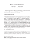
Part of the Bigfoot project was to develop a predictive model with the goal of
solving for the optimal control coefficients. The theoretical model included parameters
for the friction of the wheel-to-ground interface, the internal friction of the geared motors
and the inertia of the motors and the robot platform. A good model would allow the robot
to use different coefficients depending on the surface it was on, and therefore use
optimized turns no matter where it was driving.
In the end, an empirical model
predicting how the robot responds to voltage differences across the wheels was used to
3
tune the controller. Bigfoot can now turn to a new course, without overshoot, in a
minimum time and maintain that course until it reaches the desired location.
The model program was written in Visual Basic which provides an interface to
test and evaluate different control coefficients. This thesis discusses the inputs, using the
program, and how well the model predicts the operation of the real platform. The
controller was tuned and the resulting turn data from the robot is presented alongside the
prediction from the model.
4
II.
A.
CONTROL THEORY AND APPLICATION
CONTROL THEORY
Feedback controllers maintain control over a process by comparing the actual
values of the controlled variables to the requested set-point and changing the manipulated
variable. An everyday example of this would be driving a car at the speed limit. The
requested set-point is the speed limit, the controlled variable is the speed of the car, and
the manipulated variable is the amount of gas supplied to the engine, see Figure 3. All
the controller operations are carried out by the driver.
Figure 3.
General controller diagram applied to the example of driving a car.
Digital or mechanical controllers can replace the operations carried out by the
driver, in this example. There a numerous different types of controllers, but PID
controllers are one of the most commonly used. PID controllers serve as a simple and
flexible method of autonomously controlling a system, (Riggs, 213). Proportional control
simply relates the set-point to the actuator by a constant. This is the simplest form of
control, but in practice it often has a steady state error because it is a linear controller
applied to a system that is almost always non-linear. The final error will depend on how
close the change is to the controller’s tuned set-point. Integral control minimizes the
integral of the error over the time step of the system. If a steady state error exists, the
integral of the error will build up over time and eventually influence the controlled
5
variable to eliminate the offset. The time step is the time is takes to go one time around
the control loop (in Figure 3), and depends on the system. Derivative control impacts
how fast the controlled variable changes. This can be used to limit the response from the
controller so that the system does not continually overreact to changes or error. Each part
of PID control can be used individually or in any combination, depending on the system.
The full control equation including all three control types is shown in Equation 1. In
Equation 1, C(t) is the controlled variable and e(t) is the error at time t. Changes to this
value depend on the proportional coefficient, Kc, the integral coefficient, τI, and the
derivative coefficient, τD. The coefficient of each term can be simplified so that Kc = KP,
Kc/ τI = KI, and Kc/ τD = KD. In the model and robot code these are the values set to
optimize course control.
t
⎡
1
de(t ) ⎤
C (t ) = Co + K c ⎢e(t ) + ∫ e(t )dt + τ d
⎥
τI 0
dt ⎦
⎣
Equation 1.
The complete time form of the control equation.
Different pieces of hardware must work together to get the robot to move in the
correct direction. The control process as it applies to the robot is shown in Figure 4.
Figure 4.
Control diagram relating the hardware to the process.
All control operations are carried out by a BL2000 microprocessor. The actuators
on the robot are the motor drivers. These determine the direction and speed the motors
turn. The process is the interaction between the four motors driving the robot, the mass of
the robot and the surroundings.
The sensor is an electromagnetic compass, which
provides heading information to the processor.
6
The controlled variable can be treated as an oscillator, and will have three
possible outcomes from tuning. The system can be under-damped, critically damped, or
over-damped. Critical damping represents the fastest correction that can be made without
having an overshoot. Figures 5, 6, and 7 show how the controlled variable approaches
the setpoint for the three possible damping factors. These plots show how a simple
oscillator responds to different damping factors. Damping can come from the controller
or from the surroundings through friction.
For the robot, the controlled variable is the
voltage signal sent to the motor drivers. The error is the difference between the desired
heading and the current heading.
Underdamped Response: Damping Factor =.1
Controlled Variable
1.0
0.5
0.0
0
1
2
3
4
5
-0.5
-1.0
Time
Figure 5.
An under damped system.
Critically Damped Response: Damping Factor =1
Controlled Variable
1.0
0.8
0.6
0.4
0.2
0.0
0
1
2
3
Time
Figure 6.
A critically damped system.
7
4
5
Underdamped Response: Damping Factor =4
Controlled Variable
1.0
0.8
0.6
0.4
0.2
0.0
0
1
2
3
4
5
Time
Figure 7.
B.
An over damped system.
TUNING CONTROLLERS
The purpose of tuning controllers is to minimize deviations from set-point,
maintain the set point, avoid excessive variation of manipulated variables, and eliminate
offset (Riggs, 253). Since it is impossible to completely satisfy all of the above criteria, a
balance must be reached that is unique for the system and based on the required
performance attributes. For example, systems that utilize valves to make set-point
changes can be worn out quickly by both excessive change, and hitting the maximum
open and closed positions often. The robot differs from this type of system in that
changing the voltage to the motors often does not affect the life of the platform. Since
some voltage signal is always being sent, properly controlling the course involves
varying the existing signal. This system has a +/- 5 degree uncertainty because of the
compass, so a small offset is not a problem. However, a quick response is desired, and
oscillations must be avoided to conserve battery power. Smarter driving means less time
and energy spent getting to the destination, and more time and energy to do the mission
once there.
If the controller is not optimized properly, the robot could have sustained
oscillations or become unstable and the error will grow. The ultimate goal is to
incorporate and tune a controller that corrects the course in a critically damped manner
for all turns on all surfaces.
8
There are a number of different methods to tune controllers. Some methods are
mathematical; others involve guidelines from the numerous applications of such
controllers. It is also possible to empirically test until optimum values are found, although
this can be tedious. While tuning the robot’s controller, the initial values were based on
general guidelines and then tuned with empirical testing both on the robot and the model.
Tuning this way was possible only because the testing can be done very quickly with the
software model. If new controller coefficients had to be tested using the robot it would
take much longer and another method would be needed.
C.
OTHER INDUSTRIAL APPLICATIONS
PID controllers are commonly used in industrial processes because of their
flexibility, ease of use, and robustness.
Cruise control on cars, vehicle suspension
systems, tank level and temperature are some examples of places where PID control has
been used. PID controllers can be mechanical in nature or software based in digital
control systems. The first applications of PID control were through pneumatic controllers
in chemical processing industries in the 1930’s (Riggs, 213).
In certain circumstances, PID control does not provide a robust enough control
mechanism, so model predictive control (MPC) is used instead of, or in addition to PID
control. These circumstances are when there are there is a long time delay; major
nonlinearities; large and frequent disturbances; multivariable interactions; or constraints
on the system (Miller, 1). In large industrial plants there may be hundreds or thousands
of control loops, many of which interact with each other. Modeling and efficient control
is an economic necessity for these plants. The industrial application of PID control is not
that different from applying the same concepts to the robot, only some different tools
(types of control) are used and companies spend years developing both theoretical and
empirical models of such plants.
9
THIS PAGE INTENTIONALLY LEFT BLANK
10
III.
HARDWARE
Systemic error that exists will lead to some difference between the model and
how the real robot performs. This is why the bearing predicted by the model does not
exactly match what really occurs and why a +/- 5 degree course is acceptable. The
systemic error comes from the hardware that works to make the robot turn. For a more
in-depth explanation of all the hardware, see John Herkamp’s thesis, (Herkamp, 11-35).
A.
PROCESSOR
The BL2000 microprocessor (Figure 8) runs a Dynamic C program code,
modified for Bigfoot by John Herkamp (Herkamp, 36). The microprocessor operates at
22.1 ΜΗz and calculates the desired course based on the coordinates sent by the operator
and the GPS unit. In addition to controlling the motor speed, the processor takes in
information from the sensors and communication router and carries out other operations.
Obstacle avoidance, camera operation, thermal
sensor,
communication are all things the processor controls.
Figure 8.
BL2000 microprocessor
11
arm operations,
and
B.
MOTOR DRIVERS
The motor driver takes the voltage signal sent by the controller and converts it to
a pulse width modulated signal. The motor driver is a 50 V, 20A H-bridge motor driver.
The advantages of this type of motor driver are that none of the components have a
continuous current stress and it can drive the motor forward or in reverse at varying
speeds. Within an H-bridge circuit the resistances are varied so that different amounts of
current flow a through the motor in the desired direction, see Figure 9. In Figure 9, when
the resistance through R1 and R3 is the lowest, the motor will run in one direction, but
when the resistance R4 and R2 is the lowest the motor will turn in the opposite direction.
Variable amounts of current are sent by controlling the resistance. In practice transistors
replace the resistors to variably control the flow of current.
Figure 9.
An H-bridge circuit diagram.
12
Figure 10.
C.
H-Bridge motor driver (From Superdroid Robots).
MOTORS
The motors are powered by a 24 V nickel-metal hydride battery. An independent
battery powers all the electronics on board. The motors (Figure 11) have a loaded turn
speed of 190 rpm, a torque of 0.5 N-M, and operate at a current up to 900mA. The
motors can drive the robot, which has a mass of 11.8 kg, at about 3.8 MPH, which is a
fast walking pace. With the batteries on board the motors can drive for about 2 hours,
depending on conditions and use.
Figure 11.
D.
Drive motor (From Superdroid Robots).
ELECTRONIC MAGNETIC COMPASS
Once all these parts work together the robot drives along a new course. The
sensor that measures that course is an electronic magnetic compass, shown in Figure 12.
13
Figure 12.
Electronic magnetic compass (From Superdroid Robots).
The compass uses a magnetoresistive sensor. Resistance of certain magnetic
materials will change under the influence of an external magnetic field. In this case the
external field is that of the Earth. Figure 13 shows a diagram of how the magnetic field
and resistance are related. H represents the magnetic field of the earth and will influence
the magnetization of the plate. The resistance in the permalloy varies according to
Figure 13.
ne
t
α
M
ag
H
iz
a
tio
n
Equation 2.
Magneto resistive effect.
.
R = Ro + ∆Ro cos 2 α
Equation 2.
Resistance in the permalloy.
14
Four of these plates are arranged in a Wheatstone bridge configuration. Each
rectangle represents one of the plates shown in Figure 14. The voltage drop across +Vo
to –Vo is the signal that provides the measure of heading. The voltage across Vcc to GND
is the applied voltage from the power source.
Figure 14.
Bridge configuration for magneto resistive effect. (Philips Semiconductors)
To account for other magnetic fields present due to the robot’s electronics, the
compass was calibrated manually by aligning to magnetic north. Once the calibration
was complete, the compass aligned magnetic north along the same direction as the other
compass, and showed the correct heading for the cardinal directions. Without calibration,
the compass does not even read 90 degrees between the cardinal directions properly. The
compass sends out an 8 bit signal, and therefore has 256 possible values. Dividing 360
degrees by 256 possible outputs means the compass is precise to 1.4 degrees, as it is
implemented here. It is possible to get the compass to operate at +/-.1 degrees with a
pulse width modulated signal, but that involves significant software modifications and
would not be very helpful since the GPS is only accurate to commercial specifications.
For a complete description of all the hardware capabilities and how the hardware
was incorporated into the robot see Herkamp, pages 11 to 35.
15
THIS PAGE INTENTIONALLY LEFT BLANK
16
IV.
A.
DEVELOPMENT OF THE MODELING EQUATIONS
BASIC CONCEPTS
When the robot moves, the motion can be a combination of both forward
translational movement and rotational movement. There are two options for making
course corrections, stopping to turn or turning while driving. The first is a pivot turn and
the robot drives in a straight line until it reaches the waypoint, or until enough error is
built up, then stops and turns using reverse motion one side and forward motion on the
other side. This type of turn is faster, but the overall process is much slower and puts
unnecessary wear on both the motor controllers and wheels, because they are switching
directions often. The other option, a differential turn, is to slow one side down while
continuing forward motion. Figure 15 shows the two types of turns. Each type of turn
can be useful, depending on the circumstances. For instance turning the robot in place to
look at something or turning in tight spaces requires a pivot turn, but when making small
adjustments while driving to a new destination it is more efficient to use a differential
turn.
(A)
Figure 15.
(B)
Types of turns: (A) differential and (B) pivot.
17
B.
PRELIMINARY THEORETICAL MODEL
The original goal was to develop a widely applicable model of the how robots
turn that depended only on inertia and friction, and from which the optimal control
coefficients could be solved for. The basic idea was to start with the equation of motion
for the motors (modeled as one motor) and work through the influence of friction and
inertia and the control coefficients to a final equation of motion for the platform; resulting
in the equation of motion for the optimized turn of the robot, based on proportional and
derivative control coefficients, inertia, and friction.
Equations 3 through 9 show the development of the theoretical model. Equation 3
is the equation of motion for the motor and can be equated to the torque from the
controller. Tm is the torque of the motors, J in the inertia term, and F is the friction term.
Theta represents the course heading.
TM = Jθ + Fθ
Equation 3.
Equation of motion for the motors.
TM = K e (θ 0 − θ ) − K dθ
Equation 4.
Torque due to the controller.
In Equation 3, Ke is the combination of the proportional relationship between the
voltage to the motor and the proportional relationship between the heading error that
exists and the current to the motor. Kd is the derivative feedback coefficient. By equating
these two relationships is it possible to solve for solutions in terms of θ.
− K eθ − K dθ = Jθ + Fθ
set θ 0 = 0
Jθ + ( F + K d )θ + K eθ = 0
Equation 5.
Combined equation.
θ = θ o eq⋅t
Equation 6.
Proposed solution.
18
By taking the first and second derivative of Equation 6 and substituting into
Equation 5, the quadratic Equation 7 is the result, and the standard quadratic equation can
be used to find solutions.
K
⎡ F + Kd ⎤
q2 + ⎢
q+ e =0
⎥
J
⎣ J ⎦
Equation 7.
Quadratic equation of proposed solution.
2
⎡ F + Kd ⎤ 1 ⎡ F + Kd ⎤ 4Ke
q = −⎢
⎥±
⎢
⎥ − J
⎣ 2J ⎦ 2 ⎣ J ⎦
Equation 8.
Solutions for q using the quadratic equation.
The solution for θ is shown in Equation 9. When ω = 0 then system will be
critically damped.
θ = θoe
( − 1 α t ) ( − 1 ωt )
2
2
e
2
⎛ F + Kd ⎞
⎛ F + Kd ⎞ 4Ke
α =⎜
⎟ ω= ⎜
⎟ −
J
⎝ 2J ⎠
⎝ J ⎠
Solution for θ.
Equation 9.
Two problems existed with this approach; one is that it did not accurately predict
what the robot really did and the second being that it could only model a pivot turn. The
prediction was not accurate because the turn rate predicted by the Equation 9 was much
greater than the maximum turn of the robot. The turn rate is the slope of the turn line
shown in Figure 16. A pivot-turn has limited application since it is only part of how the
robot turns, and is used less often than the differential turn. Figure 16 shows how the
theoretical model matched the real data.
19
Theorectical Model Vs. Robot Error (Pivot Turn)
Robot
Model
120
Heading
Error(deg)
100
80
60
40
20
0
0
500
1000
1500
2000
2500
3000
3500
Time (ms)
Figure 16.
The theoretical model versus real data.
One reason the theory did not work was that it turned at twice the maximum turn
rate of the robot. By looking a the steepness of the curve in Figure 16, it can be seen that
the model predicted a turn rate that was much faster than the maximum turn rate the robot
was capable of. Because of this, the time the model said it would take to complete a turn
was half of the actual time and did not provide a way to optimize coefficients, because
the proportional and derivative control coefficients were solved for, not chosen based on
response. The coefficients required to make ω= 0 (in Equation 9), were not the optimal
coefficients. When other coefficients were used, both in the robot and in the model,
values could easily be found that were better; most likely because the influence of inertia
(J) and friction (F) were not considered correctly. Since the theoretical model did not
give a good way to control the robot an empirical model was developed to optimize the
controller.
In addition to the motors, there are two main influences on the direction of the
robot. The first is friction, which depends on what surface the robot is traveling on. The
second is inertia, including rotational inertia.
During a differential turn there is a
transition from forward motion to rotation. The robot has static friction coefficients
approaching one for most surfaces. The wheels are made of rubber, which has a higher
friction coefficient than most materials. Friction helps the wheels get traction to move, so
20
although too much friction can hinder a fast turn, it is necessary for the robot to drive.
During testing on cement, the coefficient of static friction was .96. This value was found
by pulling on the robot with a spring scale until it started moving then dividing that value
by the weight of the robot. Static friction is usually the main friction influence since the
wheels are usually turning. When the robot does a pivot turn however, the inside wheels
tend to drag, so kinetic friction contributes during a pivot turn.
C.
DEVELOPMENT OF THE MODELING EQUATIONS
Two separate tests were done on the robot to develop empirical equations that
predict how the robot would respond to applied voltage signals to the wheels. The first
test was for a pivot-turn, where the wheels on one side were set to a range of forward
voltages while the other was set to the equivalent reverse voltage. Testing included both
clockwise and counterclockwise turns. The turn was completed for a set time and the
total direction change was converted to a turn rate at that voltage. Table 1 shows the turn
rate for each voltage.
By applying a linear best fit line to the data, an equation was
developed to predict how many degrees the robot will turn for a given voltage signal.
Voltage Difference (V)
3.0
2.8
2.6
2.4
2.2
2.0
1.8
1.6
Table 1.
Turn Rate (deg/sec)
Right
Left
84.0
91.0
71.0
79.0
57.0
67.0
49.0
50.0
32.0
33.0
16.5
22.5
6.0
6.0
1.0
0.0
Turning rates for a pivot turn.
In the second test, the differential turn rate was measured. To test this, one side
was slowed down by a small incremental amount for a set time period, while the other
side moved forward at the normal driving speed. The turn rate was measured and another
equation was developed based on the data. Table 2 shows the turn rate for each measured
voltage for a differential turn.
This test was also completed for clockwise and
counterclockwise turns.
21
Voltage Diff.(V) Turn Rate(deg/sec)
2.5
71.2
2.3
64.3
1.5
18.2
1.4
17.4
1.3
14.6
1.2
14.0
1.1
12.2
1.0
11.1
0.9
10.9
0.8
9.8
0.7
7.6
0.6
6.8
0.5
5.9
0.4
4.8
0.3
3.6
0.2
2.0
Table 2.
Turning rates for a differential turn.
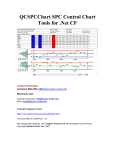
Based on the data from these tests, two equations were developed; Equation 10
for a pivot turn and Equation 11 for a differential turn. Figures 17 and 18 show how these
equations relate to data collected. The pivot turn has two curves because the robot veers
when driving straight. The robot veers due to slight voltage differences and misalignment
of the motor mounts. The misalignment pushes it when turning left and slows it when
turning right. No difference in turn rate depending on the direction was noticed for a
differential turn, probably because the misalignment is not significant enough to
influence the slower turn. The error bars represent +/- 1.4 degrees, the accuracy of the
electronic compass.
22
100.0
90.0
80.0
70.0
60.0
50.0
40.0
30.0
20.0
10.0
0.0
1.0
1.5
2.0
2.5
3.0
3.5
Left Turn
Voltage Difference (V)
Figure 17.
Right Turn
Pivot turn rate versus voltage difference.
TRight (° / sec) = 62.2i(∆V ) − 103
TLeft (° / sec) = 68.6i(∆V ) − 114
Equation 10.
Model equation for a pivot turn.
Differential Turn Rate Vs. Voltage Difference
25.0
Turn Rate (deg/sec)
Turn Rate (deg/sec)
Pivot Turn Rate Vs. Voltage Difference
20.0
15.0
10.0
5.0
0.0
0.0
0.2
0.4
0.6
0.8
1.0
1.2
1.4
Voltage Difference(V)
Figure 18.
Differential turn rate versus voltage difference.
23
1.6
T (° / sec) = 12.00i(∆V ) − 0.28
Equation 11.
Model equation for a differential turn.
When the robot first starts turning it has to overcome inertia and friction. This was
modeled in the software by limiting how fast the model could “turn” in the first three
time steps. For a pivot turn the initial turn rate was limited to 2 degrees per time step for
the first three time steps and was based on experimental turn data. For a differential turn
the limit was set to 4 degrees for the first three time steps, which was also observed
during testing.
There is a range of voltages in which the robot does not have enough power to get
going or stay going. To start moving, the motors must overcome static friction and
inertia, and to keep the robot moving there must be enough power to overcome kinetic
friction. The minimum voltage needed to get the robot going is the static stall voltage,
and will be greater than the voltage required to turn the motor when no load is applied.
The voltage required to keep the robot moving is the kinetic stall voltage. To determine
what these were, incrementally lower voltages were sent to the motors until the robot
could not keep moving, or in the static case could not start moving. The stall voltage was
modeled by setting the course change to zero when the controller calls a voltage below
the stall voltage. Stalling occurred primarily during pivot turns. Integral control becomes
the only factor that influences the voltage when the stall voltage is reached, because the
integral of error will have to build up before any change will be called that is above the
stall voltage. Table 3 shows the stall voltages.
Stall Voltages:
Static
Forward
2.3
Reverse
2.8
Table 3.
Kinetic
2.4
2.6
Stall voltages.
Equations 10 and 11 and the information from Table 3 are applied to the third step (Robot
or Model) in the Robot Control loop as displayed in Figure 19 below. The adjusted motor
control voltages are the entering argument for this step and the development if this
parameter is discussed next.
24
D.
COURSE CONTROL
The model we develop here provides an empirical prediction of how the robot
turns based on adjusted motor control voltages as a function of heading error. The model
also provides a method of optimizing PID steering control coefficients for our platform. It
could be applied to other platforms with similar physical characteristics. These
characteristics would include any two or four-wheeled robot with a motor controller for
each side, including robots with a tank tread. Three-wheeled robots or any other omnidirectional platform would require some code modifications.
Figure 19 shows a diagram of how initial course information is converted into a
usable voltage signal to the motors. The desired heading, calculated by the processor, is
compared to the current heading, measured by the sensor. The result gives an error, a
number, between the actual and desired heading. The error is transformed to a
dimensionless scaled voltage signal according to the equations derived from Figure 20.
That scaled voltage signal is then adjusted by a PID control transform in order to avoid
overshoot and offset. The adjusted voltage signal then goes to the motor drivers, which
sets the actual voltage (not dimensionless) to the motors. The motors turn, and the robot
comes to a new heading. Then the whole process starts over.
Figure 19.
Robot Control Schematic
25
1.
Turning Voltage
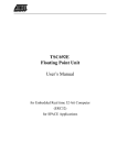
Figure 20 shows how heading error is converted to the scaled voltage signal for
the left and right motors. The vertical axis represents the range of voltages from the
BL2000 to the motor controller. . The horizontal axis is the calculated error, and is the
difference between the desired and actual heading of the robot. We define the 2.5-volt
intercept for the left and right motor as the stop voltage. On the figure, voltage values
between 1 and 2.5 volts indicate a reverse direction for the applicable motor, while
voltage values that fall between 2.5 and 4 volts would specify a forward direction. For
example, a 60-degree positive bearing error would indicate a 2-volt signal to the right
motor and a 3-volt signal to the left. Since 2-volts falls between 1 and 2.5 the right motor
would turn at a medium speed in the reverse direction. Similarly, the 3-volt signal falls
between 2.5 and 4 and would specify a medium forward speed for the left motor.
Consequently the robot would make a pivot-turn to the right at medium speed.
Voltage(V) Vs. Error(deg)
4.0
3.5
Voltage (V)
3.0
2.5
2.0
1.5
1.0
-180
-140
-100
-60
0.5
-20
20
60
100
Error (deg)
Figure 20.
Error to Motor Control Voltage Conversion
26
140
180
The equations of the lines for Figure 20 are shown in Equation 12. Pink is the
voltage to the right motor, blue is the voltage to the left motor, when the error is the
desired course minus the current course, as it is in the code. They are used in the Visual
Basic algorithm, to calculate the applicable voltages based on error. The slope of the
voltage-error line (m voltage slope) is the total range of voltage, Vmax-Vmin, (1.5 V) divided by
the total possible error (180º). The intercept must be the stop voltage (2.5 V) so that
when no error exists the robot will stop turning. Vright and Vleft are the voltages needed to
do a pivot turn to eliminate the error Eº.
mvoltage slope =
Vmax − Vmin 1.5
=
Emax − Emin 180
Vright = 2.5 − .00833 ⋅ ( E )
Vleft = 2.5 + .00833 ⋅ ( E )
Equation 12.
2.
Equation of the lines.
PID Adjustment to Voltage
The next step in our control loop is to apply the PID transform, a code version of
Equation 1, to the scaled voltage signal just calculated.
Since the PID control used here scales the actual voltage signal based on Figure
20, the KP and KI and KD control coefficients are all unit-less. The actual control
equation, which includes the PID coefficients, programmed into both the robot software
and the model software is shown in Equation 13. Pscale, iscale and dscale are the equivalent of
error from Equation 1, in terms of voltage. The Eºold- Eºnew represents the change in
heading during one loop through the process.
27
Vinside = 2.5 + (K P ⋅ pscale + K I ⋅ iscale + K D ⋅ d scale )
pscale = (E° ⋅ 0.00833)
iscale = pscale + iscale
d scale = ( (E °old -E ° new ) ⋅ 0.00833)
1.5
(converts E° to volts)
180
E ° = error in degrees
.00833=
Equation 13.
Control equation used in the robot and the model.
The control equation calculates the voltage to the inside wheels. The voltage set
for the outside wheels depends on the type of turn being completed. For a pivot turn the
outside voltage was set to five minus the inside voltage, and for a differential turn the
outside voltage is set to one, the full forward speed.
3.
Systemic Error
Certain limitations arise from the components and reality of the system. Some of
these can be adequately transferred into the model; however some simply contribute to
error between the model and the robot. If the error between the model and the real system
is small enough, then the model can be used to predict the response of the real system to
the tuning coefficients and the controller can be optimized easily.
One of the limitations is a dead band limitation in the motor controllers. At 2.5 V
±2.5% the motor will stop. Using this information the minimum error can be calculated.
This is simulated within the model by setting the maximum error in the code. Equation
14 shows how the maximum accuracy of the motor controllers is calculated.
maximum error in the model and in the software to run the robot was set to 5º.
28
The
Db = 2.7%
Db ⋅ Vrange = Vaccuracy
±.027 ⋅ 2.5 ⋅
e =
1
= ±.034
2
Vaccuracy
mvoltage slope
.034 ≥ .00833 ⋅ e
e =
.034
= 4.1
.00833
Equation 14.
Error due to dead band.
In Equation 14 the voltage dead band (Db) is 2.7% for the motor controllers, from
the manufacturer specifications. The possible voltage range is 2.5 V, so the voltage dead
band on either side of the stop voltage (2.5 V) is .034. Using the slope from the voltageerror equation (m
voltage slope)
(Figure 20) this can be converted to how many degrees the
motor controllers will be accurate to (eº).
In addition to the stop voltage dead band, there is also a stall voltage limitation.
The stall voltage is defined as the applied motor voltage required too overcome robot
friction and inertia. Table 3 shows the stall voltages, and a discussion of how they were
modeled is addressed in the modeling equation section. The robot also veers left at a rate
of about 1degree per 5 yards, which influences pivot turns, but not differential turns.
Another limitation is that the electronic compass has only 256 possible values. So
instead of representing a circle with 360 degrees, the compass can only choose one of 256
values, therefore each compass value corresponds to about 1.4º. After the conversion, the
heading is an integer value, whereas the course calculated from the GPS data is
continuous to three digits.
E.
PROGRAM DEVELOPMENT
1.
Program Inputs
The modeling program developed provides an easy and quick way to test control
coefficients for the robot, and could easily be applied to other platforms with some small
29
modifications in code. The user enters into the program an initial heading, a desired
heading, and the PID coefficients to be tested. Figure 21 shows a screen shot of the
program. The program for the differential turn looks the same, except for different titles
and a different picture showing the type of turn that is being modeled.
Figure 21.
Modeling program interface.
All the input boxes (shown in Figure 22) are open, and all need a value. Output
values are not in a box. If one type of control is not going to be used, a zero is entered in
the space for the coefficient.
Figure 22.
Modeling software inputs
30
Controlling the program is user friendly and done using the command buttons
shown in Figure 23. The “Go!” command is used to start the program once all the inputs
have been entered. The “Export” button copies the data plotted in the charts the to
computer clipboard so it can be pasted into another application (i.e. Excel) allowing the
model to be compared to real data. The “Quit” button ends the program.
Figure 23.
Program commands.
The proportional and derivative control coefficients were chosen to critically
damp the system. Some general rules exist to establish a starting point when choosing
control coefficients (Cabezas, 15). These are:
•
Set the integral gain to zero
•
Set the proportional gain to a reasonable starting value (KP)
•
Set the derivative gain (KD) to twice the KP
Following these guidelines, the initial values for KP and KD were chosen to be 1 and 2,
respectively and later adjusted. This uses the initial voltage calculation that is only based
on error, but with a limit on how much voltage change can be made.
The iterative process of setting the voltage, calculating the response, and setting
another voltage is within a “while” loop, in the Visual Basic code. The model calculates
current error and updates the animation, table, and charts for the current heading. Then a
new voltage is calculated based on the error and the control coefficients and the predicted
response determines the new heading. Then the whole process the repeats. For the exact
modeling code, see Appendix 1 and 2.
31
The Visual Basic language was chosen so that the end product can easily be used
by a person with little knowledge of computer programming. If the theoretical model had
been used instead of the empirical model, the user would only need to know the inertia
and friction of the platform to be able to optimize the controller. The empirical model is
more user friendly than a MATLAB or C program, where the user would have to be very
familiar with that language/ software to use the model. Visual Basic provides a way to
view the information and export the data as well as any of these other software options.
The disadvantage of Visual Basic, at least with the version used here, is that it does not
handle imaginary numbers easily. This may have been a contributing factor in why the
theoretical model did not fit the real data well.
2.
Program Outputs
There are three ways of interpreting the calculations completed within the model:
an animation, a table, and two charts.
The animation, Figure 24, shows a visual
simulation of how the robot will turn. The blue line represents the front of the robot, and
will be pointed in the direction the robot is driving. The top of the page represents 0/360
degrees or due north, just like the top of a map represents north.
Figure 24.
Model animation.
The table shows the current heading and desired heading for each time step. The
robot takes approximately 340 ms to cycle through the reading of the compass,
calculations, data output, and output of new voltages to the motors, therefore the model
calculates the heading at the same 340 ms interval. Figure 25 shows the data table from
the modeling software.
32
Figure 25.
Model data table.
Along the right side of the program window there are two charts. The charts show
the actual heading and the heading error. The heading error chart has proven to be the
most useful since it is not subject to jump across 0 to 360.
Figure 26.
Chart output from the modeling program.
For a workable configuration of inputs, the error should approach zero. Error will
always be less than 180º, since both the robot and the model are programmed to turn
towards the direction with the smallest error. Using the export function within the
program, the error data can be copied to the clipboard, and can be plotted alongside data
from the robot. Figure 26 shows the error plot for a modeled turn. Also, at the top of the
inputs section there is a “time elapsed” value that shows once a turn has been completed.
33
This is how long it took for the error to become less than 5 degrees, and provides a quick
way to tell if one set of coefficients is better than another.
Often, multiple sets of coefficients will give the same output. This means that
they all maximize the turn rate of the robot, which will optimize the turn. It is best to use
the smallest coefficients possible that maximize the turn rate of the robot, in order to
decrease the chance of overshoot, or the robot becoming unstable. Overshoot almost
always leads to sustained oscillations in this system, because the system would constantly
overshoot back and forth by the same amount. Derivative control will decrease the
likelihood this will occur. The robot did this at times and would constantly search for the
heading, going back and forth across it, but never finding it. The width of the oscillation
is based to the minimum correction from Equation 12 and did not die out because even
the minimum correction caused overshoot and the influence of the PID coefficients did
not have any affect.
34
V.
A.
IMPLEMENTATION AND EVALUATION OF THE
CONTROLLER
OPTIMIZATION AND TUNING
Each system has unique criteria for an optimized controller. The key criteria for
this platform were to minimize the turn time and eliminate any large oscillations. Small
oscillations can be tolerated within the limitations of the robot (+/- 5 degrees). In both
the robot software and the model once the error is less than five degrees, the voltages are
set to 2.5 V (stop voltage) for a pivot turn and 0.1 V (full forward) for a differential turn.
This is a fairly large window, and could lead to a significant distance error from the
destination if that course was followed the whole way.
However, since the robot
continually updates the course needed to reach the destination the error between the
desired course and the current course eventually grows beyond 5 degrees, and a new turn
will be initiated. The robot will travel shorter distances along any particular course as it
nears the destination, but will stop when it comes within 4.6 meters, due to limits in GPS
accuracy. Also, once the robot gets close to the final destination it is expected to be put
in manual mode. The optimized coefficients for each turn are shown in Table 4 along
with the time it takes to complete the turn. Integral control was not needed for a
differential turn since the only systemic error observed was less than 5 degrees.
KP
1
1
Differential
Pivot
Table 4.
B.
KI
0
5
KD
3.5
3
Turn Time (Sec) (170 deg)
Robot
Model
5.4
5.1
4.0
4.0
Optimal Coefficients and Corresponding Turn Times
EVALUATION
To determine how well the model matched the real platform, the robot was
programmed to make the same turns plotted with the model while recording heading data
with each calculation. This was done with the same controller coefficients entered into
the robot software as were input to the program. In Figures 27 through 30, below, the
heading error versus time is shown for a 170 degree turn and a 90 degree turn for both
35
pivot turns (Figures 29 and 30) and differential turns (Figures 27 and 28). The particular
turns were chosen because turns of approximately 90 degrees are commonly used in
reaching the desired destination, and a turn of 170 degrees is close to the maximum.
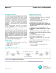
The optimal coefficients from the model did give the fastest turns for the robot,
and no noticeable oscillations were observed. Other coefficients were tested in the robot
software to see if there were any that would make the robot complete the turn faster, and
none were found.
Optimized Differential Turn: 170 deg
KP=1, KI=0, KD=3.5
Heading Error (deg)
200
run 1
run 2
run 3
model
150
100
50
0
0
1000
2000
3000
4000
5000
6000
7000
Time(ms)
Figure 27.
Optimized differential turn, model and real data (170 degree turn)
36
Optimized Differential Turn: 90 deg
KP=1,KI=0, KD=3.5
Heading Error(deg)
100
80
run 1
run 2
run 3
model
60
40
20
0
0
1000
2000
3000
4000
5000
Time (ms)
Optimized differential turn, model and real data (90 degree turn)
Figure 28.
A slightly different model was used to simulate a pivot turn, because the voltage
set on the outside wheels is 5V minus the inside voltage, but for a differential turn the
outside voltage is set to 1 V (full forward). Figures 29 and 30 show optimized turn data
for pivot turns of 178 and 90 degrees.
Optimized Pivot Turn: 178 deg
KP=1, KI=5, KD=3
Heading Error(deg)
200
150
run1
run2
run3
model
100
50
0
0
1000
2000
3000
4000
5000
Time (ms)
Figure 29.
Optimized pivot turn, model and real data (178 degree turn)
37
Heading Error (deg)
Optimized Pivot Turn: 90 deg
KP=1, KI=5,KD=3
100
80
model
60
run1
40
run2
run3
20
0
0
500
1000
1500
2000
2500
Time(ms)
Figure 30.
Optimized pivot turn, model and real data (90 degree turn)
The model does not exactly match what the robot does, because the fit used to
approximate the turn is linear, whereas the turn is not really linear. The model was
usually off by less than ten degrees at any given point. The time required to complete the
turn that is reported by the program was off by 6%. Most importantly, the optimized
coefficients in the program were also the optimized coefficients for the robot. Also, the
maximum turn rate in the empirical model matched the maximum turn rate that was
observed while testing the robot. There are many factors that change performance which
were isolated to minimize error between the model and the platform. For example, even
the charge on the battery affects how the robot turns. To minimize the influence of other
factors, the robot was always tested on the same surface and on a full battery charge. The
usefulness of the results is limited though, since the robot can operate on many different
surfaces, even sloped ones, and will always have a changing battery charge.
The
different coefficients are used in the robot code based on the type of turn. When
navigating to a new waypoint the robot uses the differential turn coefficients, but when
the robot is in manual control and the operator enters a new direction to face in the
graphical user interface (GUI) the pivot turn coefficients are used.
38
C.
IMPROVED PERFORMANCE
The next step to improve how the robot changes direction would be to incorporate
a steering mechanism on one or both sets of wheels, so the robot turns more like a car and
less like a tank. While the hardware for this would be more complicated, it would have
certain advantages. A control process may not even be necessary. A rotating servo
would simply turn a set of wheels to the heading requested. The disadvantage would be
that the robot could not pivot turn in place, unless a combination of steering systems were
used. For some platforms or missions, the ability to turn in place may not be important.
In addition to different hardware, if a theoretical model was perfected, the robot
could choose different control coefficients based on data it collects about its
surroundings, or information sent from an operator during the initial mission load. No
empirical model will model the system perfectly since conditions change constantly, but
a good model should provide useful information about what the model does and how it
responds, which this does.
39
THIS PAGE INTENTIONALLY LEFT BLANK
40
VI.
A.
CONCLUSION AND FUTURE WORK
APPLICATION TO OTHER PLATFORMS
The model developed for this platform could easily be applied to any other two or
four wheeled robots that are reasonably similar to the one tested.
New optimal
coefficients could then be determined. The two things that would need to be changed in
the model are the voltage limits and the equation that relates voltage difference to turning
rate. The voltage limits are determined by the motor controller used on the new platform
tested. The equations that relate voltage difference to turning rate can be found by
measuring a change in heading for voltage difference from one side to the other in the
usable voltage range. Then by applying a best fit equation that adequately represents how
the robot turns, the platform response to a given voltage can be predicted.
Two simple tests would be enough to modify this model to another platform.
One is a turn rate versus voltage difference for differential turn and the other is a turn rate
versus voltage difference for a pivot turn. The initial turn limits can also be observed
during these tests and adjusted. If a theoretical model were to be developed only the
inertia and friction (platform and terrain dependent) of the platform would need to be
entered, instead of the empirical equations.
This same process and the format of the software could also be applied to other
industrial processes other than robots in situations where PID control is applicable. The
whole process of modeling the response to an input and controlling that input is the same
as the process used for this model and robot. A computer program can be very useful in
tuning the controller and evaluating the model.
B.
IMPROVING THIS WORK
It is possible to develop a theoretical equation of motion that governs the robot.
The theoretical models that were developed as a part of this project did not match what
the robot was doing well enough for any effective controller to be developed, most likely
because the theoretical model involved imaginary numbers which are difficult to program
in Visual Basic. It is also possible to incorporate control coefficients into the equation of
41
motion and solve for the optimized values. The equation of motion will need to include
static friction for the rolling of the wheels, and in the case of a pivot turn will need to
include kinetic friction since the wheels drag during this type of turn. The other main
input into any theoretical model will have to be both the inertia of the platform and the
inertia of the motors, which are acting in perpendicular planes. The equation would have
voltage to the motors as the independent variable with a turning rate as the dependent
variable.
Another aspect of this work is that the robot could potentially need different
optimized coefficients if it is driving on different surfaces, such as grass, sand, cement, or
gravel. The ultimate goal would be to have a theoretical model that can be used to
determine control coefficients for different robots traveling over different surfaces,
allowing the robot to choose a different set of coefficients depending on the type of
surface it is traveling over.
42
APPENDICES
A.
APPENDIX 1: DIFFERENTIAL TURN MODEL CODE IN VISUAL
BASIC
'ROBOT MODELING AND CONTROL
'ENS Todd Williamson June 2007
'Differential Turn
Dim t As Double
Dim values() As Double
'array for heading data
Dim errors() As Double
'array for error data
Dim i As Double
'counter for array loops
Dim flag As Boolean
'flag for turn direction: true= right turn, false=left turn
Dim theta As Double
Dim done As Boolean
Private Sub END_Click()
End
End Sub
Private Sub Export_Click()
MSChart2.EditCopy
End Sub
'copies the ERROR charts and data to the clipboard
'to paste into another program
Private Sub Form_Load()
done = False
'resets counter for new turn
oldCEB = 0
'sets error for derivative control to zero
ReDim values(1 To 2, 1 To 1000)
'clear bearing array
For i = 1 To 1000
values(1, i) = 0
values(2, i) = 0
Next i
ReDim errors(1 To 2, 1 To 1000)
' clear error array
For Z = 1 To 1000
errors(1, Z) = 0
errors(2, Z) = 0
Next Z
MSChart1.ChartData = values
' clear default data out of bearing chart
MSChart2.ChartData = errors
' clear default data out of error chart
MSChart1.ShowLegend = False
' sets up chart to view data
MSFlexGrid1.Rows = 1
MSFlexGrid1.Cols = 3
' A bunch of stuff to set up the table
MSFlexGrid1.ScrollTrack = True
MSFlexGrid1.ColAlignment(1) = flexAlignLeft
MSFlexGrid1.ColAlignment(2) = flexAlignLeft
43
MSFlexGrid1.ColWidth(0) = 1000
MSFlexGrid1.RowHeight(0) = 500
MSFlexGrid1.ColWidth(1) = 1200
MSFlexGrid1.ColWidth(2) = 1200
MSFlexGrid1.WordWrap = True
MSFlexGrid1.Row = 0
MSFlexGrid1.Col = 0
MSFlexGrid1.Text = "Time (ms)"
MSFlexGrid1.Row = 0
MSFlexGrid1.Col = 1
MSFlexGrid1.Text = "Current Heading (deg)"
MSFlexGrid1.Row = 0
MSFlexGrid1.Col = 2
MSFlexGrid1.Text = "Setpoint (deg)"
MSChart1.chartType = VtChChartType2dXY
End Sub
Private Sub run_Click()
ReDim values(1 To 2, 1 To 1000)
' clear bearing array
For i = 1 To 1000
values(1, i) = 0
values(2, i) = 0
Next i
ReDim errors(1 To 2, 1 To 1000)
' clear error array
For Z = 1 To 1000
errors(1, Z) = 0
errors(2, Z) = 0
Next Z
MSChart1.ChartData = values
' clear default data out of bearing chart
MSChart2.ChartData = errors
' clear default data out of error chart
t=0
temp = 0
ct = 0
done = False
CH = IH
'Sets initial Current heading
CEB1 = DH - IH
'Finds initial error
MSFlexGrid1.Rows = t + 2
'Loads initial into grid display
MSFlexGrid1.Row = 1
MSFlexGrid1.Col = 0
MSFlexGrid1.Text = 0
MSFlexGrid1.Row = 1
MSFlexGrid1.Col = 1
MSFlexGrid1.Text = Format(CH, "###.0")
MSFlexGrid1.Row = 1
MSFlexGrid1.Col = 2
MSFlexGrid1.Text = DH
44
initialCEB = CEB1
While ct < 5
'START WHILE LOOP
'Animation
simulation.Cls
simulation.DrawWidth = 5
simulation.Circle (800, 800), 400, vbGreen
If CH <= 90 Then
'Splits Circle into quadrants and sets the direction of the
line
theta = 90 - CH
theta = theta * (3.14159 / 180)
xc = 550 * Cos(theta)
yc = -550 * Sin(theta)
ElseIf CH <= 180 Then
theta = CH - 90
theta = theta * (3.14159 / 180)
xc = 550 * Cos(theta)
yc = 550 * Sin(theta)
ElseIf CH <= 270 Then
theta = 270 - CH
theta = theta * (3.14159 / 180)
xc = -550 * Cos(theta)
yc = 550 * Sin(theta)
ElseIf CH <= 360 Then
theta = CH - 270
theta = theta * (3.14159 / 180)
xc = -550 * Cos(theta)
yc = -550 * Sin(theta)
ElseIf CH > 360 Then
simulation.Print ("ERROR-HIGH")
ElseIf CH < 0 Then
simulation.Print ("ERR0R- Low")
End If
simulation.Line (800, 800)-(xc + 800, yc + 800), vbBlue
'END ANIMATION
CEB1 = DH - CH
If done = True Then CEB1 = 0
t=t+1
temp = (temp + 340)
MSFlexGrid1.Rows = t + 2
If CEB1 < -180 Then
' Picks which way to turn
CEB1 = DH - CH + 360
' wheel on the side to turn towards.
DisplayCH = Format(CH, "###.0")
err = Format(CEB1, "###.0")
flag = True
'TRUE = RIGHT TURN
ElseIf CEB1 > 180 Then
CEB1 = DH - CH - 360
45
DisplayCH = Format(CH, "###.0")
err = Format(CEB1, "###.0")
flag = False
ElseIf CEB1 > 0 Then
DisplayCH = Format(CH, "###.0")
err = Format(CEB1, "###.0")
flag = True
ElseIf CEB1 < 0 Then
DisplayCH = Format(CH, "###.0")
CEB1 = -CEB1
err = Format(CEB1, "###.0")
flag = False
End If
If CEB1 > 180 Then CEB1 = 180
pscale = (CEB1 * 0.00833)
'.00833=3/360 converts error (deg) to volts
iscale = pscale + iscale
dscale = ((CEB1 - oldCEB) * 0.00833)
insidevoltage = 2.5 - ((KP * pscale + KI * iscale + KD * dscale)) / 10
outsidevoltage = 1
If t Mod 5 = 0 Then iscale = 0
' resets integral every 5 time steps
voltagedifference = insidevoltage - outsidevoltage
CHold = CH
If voltagedifference > 1.5 Then voltagedifference = 1.5
If KP < 1 Then voltagedifference = 0
If done = True Then voltagedifference = 0
If flag = True Then
CH = CH + 12 * voltagedifference
'Response to Voltage for right turn
If temp < 1020 Then CH = CHold + 4
'limits initial turn
ElseIf flag = False Then
CH = CH - 12 * voltagedifference
'Response to Voltage for left turn
If temp < 1020 Then CH = CHold - 4
'limits initial turn
End If
While CH > 360
'while loop to keep CH below 360
CH = CH - 360
Wend
'end range while loop
While CH < 0
'while loop to keep CH above 0
CH = CH + 360
'end range while loop
Wend
'BEARING PLOT INFO
values(1, t) = (temp - 340) / 10
'Loads new values into data array
values(2, t) = DisplayCH
'ERROR PLOT INFO
errors(1, t) = (temp - 340) / 10
errors(2, t) = Abs(CEB1)
'Loads new values into grid display
MSFlexGrid1.Row = t + 1
46
MSFlexGrid1.Col = 0
MSFlexGrid1.Text = temp
MSFlexGrid1.Row = t
MSFlexGrid1.Col = 1
MSFlexGrid1.Text = Format(DisplayCH, "###.0")
MSFlexGrid1.Row = t + 1
MSFlexGrid1.Col = 2
MSFlexGrid1.Text = DH
If CEB1 < 5 Then
ct = ct + 1
End If
If CEB1 < 5 And done = False Then
TimeElapsed = temp - 340
done = True
End If
oldCEB = CEB1
If t > 50 Then
ct = 6
End If
Wend
'END MAIN while LOOP
ReDim Preserve values(1 To 2, 1 To t)
ReDim Preserve errors(1 To 2, 1 To t)
MSChart1.ChartData = values
' Sends bearing data to chart
MSChart2.ChartData = errors
' Sends error data to chart
End Sub
B.
APPENDIX 2: PIVOT TURN MODEL CODE IN VISUAL BASIC
'ROBOT MODELING AND CONTROL
'ENS Todd Williamson June 2007
'Pivot Turn
Dim t As Double
Dim values() As Double
'array for heading data
Dim errors() As Double
'array for error data
Dim i As Double
'counter for array loops
Dim flag As Boolean
'flag for turn direction: true= right turn, false=left
turn
Dim theta As Double
Dim done As Boolean
Private Sub END_Click()
End
End Sub
47
Private Sub Export_Click()
MSChart2.EditCopy
'copies the ERROR charts and data to the clipboard to paste
End Sub
‘ into another program
Private Sub Form_Load()
done = False
'sets check for end of turn to zero
oldCEB = 0
ReDim values(1 To 2, 1 To 1000)
' clear bearing array
For i = 1 To 1000
values(1, i) = 0
values(2, i) = 0
Next i
ReDim errors(1 To 2, 1 To 1000)
' clear error array
For Z = 1 To 1000
errors(1, Z) = 0
errors(2, Z) = 0
Next Z
MSChart1.ChartData = values
' clear default data out of bearing chart
MSChart2.ChartData = errors
' clear default data out of error chart
MSChart1.ShowLegend = False
' sets up chart to view data
MSFlexGrid1.Rows = 1
MSFlexGrid1.Cols = 3
MSFlexGrid1.ScrollTrack = True
MSFlexGrid1.ColAlignment(1) = flexAlignLeft ' A bunch of stuff to set up the table
MSFlexGrid1.ColAlignment(2) = flexAlignLeft
MSFlexGrid1.ColWidth(0) = 1000
MSFlexGrid1.RowHeight(0) = 500
MSFlexGrid1.ColWidth(1) = 1200
MSFlexGrid1.ColWidth(2) = 1200
MSFlexGrid1.WordWrap = True
MSFlexGrid1.Row = 0
MSFlexGrid1.Col = 0
MSFlexGrid1.Text = "Time (ms)"
MSFlexGrid1.Row = 0
MSFlexGrid1.Col = 1
MSFlexGrid1.Text = "Current Heading (deg)"
MSFlexGrid1.Row = 0
MSFlexGrid1.Col = 2
MSFlexGrid1.Text = "Setpoint (deg)"
MSChart1.chartType = VtChChartType2dXY
End Sub
Private Sub run_Click()
ReDim values(1 To 2, 1 To 1000)
For i = 1 To 1000
values(1, i) = 0
' clear bearing array
48
values(2, i) = 0
Next i
ReDim errors(1 To 2, 1 To 1000)
For Z = 1 To 1000
errors(1, Z) = 0
errors(2, Z) = 0
Next Z
MSChart1.ChartData = values
MSChart2.ChartData = errors
t=0
temp = 0
ct = 0
done = False
TimeElapsed = 0
' clear error array
' clear default data out of bearing chart
' clear default data out of error chart
CH = IH
CEB1 = DH - IH
'Loads initial into grid display
MSFlexGrid1.Rows = t + 2
MSFlexGrid1.Row = 1
MSFlexGrid1.Col = 0
MSFlexGrid1.Text = 0
MSFlexGrid1.Row = 1
MSFlexGrid1.Col = 1
MSFlexGrid1.Text = Format(CH, "###.0")
MSFlexGrid1.Row = 1
MSFlexGrid1.Col = 2
MSFlexGrid1.Text = DH
initialCEB = CEB1
oldCEB = CEB1
While ct < 5
'START WHILE LOOP
'Animation
simulation.Cls
simulation.DrawWidth = 5
simulation.Circle (800, 800), 400, vbGreen
If CH <= 90 Then
'Splits Circle into quadrants and sets the direction of
the line
theta = 90 - CH
theta = theta * (3.14159 / 180)
xc = 550 * Cos(theta)
yc = -550 * Sin(theta)
ElseIf CH <= 180 Then
theta = CH - 90
theta = theta * (3.14159 / 180)
xc = 550 * Cos(theta)
yc = 550 * Sin(theta)
49
ElseIf CH <= 270 Then
theta = 270 - CH
theta = theta * (3.14159 / 180)
xc = -550 * Cos(theta)
yc = 550 * Sin(theta)
ElseIf CH <= 360 Then
theta = CH - 270
theta = theta * (3.14159 / 180)
xc = -550 * Cos(theta)
yc = -550 * Sin(theta)
ElseIf CH > 360 Then
simulation.Print ("ERROR-HIGH")
'Shows on animation if error exists
ElseIf CH < 0 Then
simulation.Print ("ERR0R- Low")
End If
simulation.Line (800, 800)-(xc + 800, yc + 800), vbBlue
'END ANIMATION
CEB1 = DH - CH
If done = True Then CEB1 = 0
t=t+1
temp = (temp + 340)
MSFlexGrid1.Rows = t + 2
If CEB1 < -180 Then
' Picks which way to turn
CEB1 = DH - CH + 360
' wheel on the side to turn towards.
DisplayCH = Format(CH, "###.0")
err = Format(CEB1, "###.0")
flag = True
' TRUE = RIGHT TURN
ElseIf CEB1 > 180 Then
CEB1 = DH - CH - 360
DisplayCH = Format(CH, "###.0")
err = Format(CEB1, "###.0")
flag = False
ElseIf CEB1 > 0 Then
DisplayCH = Format(CH, "###.0")
err = Format(CEB1, "###.0")
flag = True
ElseIf CEB1 < 0 Then
DisplayCH = Format(CH, "###.0")
CEB1 = -CEB1
err = Format(CEB1, "###.0")
flag = False
End If
If CEB1 > 180 Then CEB1 = 180
pscale = (CEB1 * 0.00833)
'.00833=3/360 converts error (deg) to volts
iscale = pscale + iscale
dscale = ((CEB1 - oldCEB) * 0.00833)
50
insidevoltage = 2.5 + (KP * pscale + KI * iscale + (KD / 3) * dscale)
If t Mod 5 = 0 Then iscale = 0
outsidevoltage = 5 - insidevoltage
If insidevoltage > 4 Then insidevoltage = 4
If insidevoltage < 2.5 Then insidevoltage = 2.5
If outsidevoltage < 1 Then outsidevoltage = 1
If outsidevoltage > 2.5 Then outsidevoltage = 2.5
voltagedifference = Abs(insidevoltage - outsidevoltage)
CHold = CH
If voltagedifference > 1.5 Then voltagedifference = 1.5
If done = True Then voltagedifference = 0
If flag = True Then
CH = CH + 12 * voltagedifference
'Response to Voltage for right turn
If temp < 680 Then CH = CHold + 2
'limits initial turn
ElseIf flag = False Then
CH = CH - 12 * voltagedifference
'Response to Voltage for left turn
If temp < 680 Then CH = CHold - 2
'limits initial turn
End If
While CH > 360
'while loop to keep CH below 360
CH = CH - 360
Wend
'end range while loop
While CH < 0
'while loop to keep CH above 0
CH = CH + 360
'end range while loop
Wend
'BEARING PLOT INFO
values(1, t) = (temp - 340) / 10
'Loads new values into data array
values(2, t) = DisplayCH
'ERROR PLOT INFO
errors(1, t) = (temp - 340) / 10
errors(2, t) = err
'Loads new values into grid display
MSFlexGrid1.Row = t + 1
MSFlexGrid1.Col = 0
MSFlexGrid1.Text = temp
MSFlexGrid1.Row = t
MSFlexGrid1.Col = 1
MSFlexGrid1.Text = Format(DisplayCH, "###.0")
MSFlexGrid1.Row = t + 1
MSFlexGrid1.Col = 2
MSFlexGrid1.Text = DH
If CEB1 < 5 Then
ct = ct + 1
End If
If CEB1 < 5 And done = False Then
TimeElapsed = temp - 340
done = True
51
End If
oldCEB = CEB1
If t > 50 Then
ct = 6
End If
Wend
'END MAIN while LOOP
ReDim Preserve values(1 To 2, 1 To t)
ReDim Preserve errors(1 To 2, 1 To t)
MSChart1.ChartData = values
'Sends bearing data to chart
MSChart2.ChartData = errors
'Sends error data to chart
End Sub
C.
SOFTWARE USER’S MANUAL
To run the included simulation programs the MSCHART.OCX file must be
included in the folder the programs are run from. Double click the type of turn desired to
be modeled. In the opening window five inputs exist:
1. Initial heading- this is the initial direction the robot is pointed.
2. Desired heading- the direction the robot needs to face after the turn. Usually,
what is needed is a particular span of a turn- for example a 90 degree turn or a 180
degree turn. Any initial and final value can be used to give the necessary original
error.
3. Proportional- the proportional control coefficient. This coefficient is unitless since
the control only factors the original correction estimated by the robot.
4. Integral- the integral control coefficient. This will multiply the error over the last
10 time steps, and factors it into the next voltage assigned.
5. Derivative- the derivative control coefficient. This input multiplies the difference
in the last two time steps by the coefficient entered and factors it into the next
voltage signal.
Once the desired values are entered, click the “Go!” button. The program will simulate
how the robot will respond to that set of values. The chart will automatically plot the
heading versus time and error versus time data. In the top left of the screen a “Time
Elapsed for Turn” box exists. A value will show up if the turn was completed
successfully. This is the time it took for the error to come below 5 degrees and stay for
five time steps. The time shown in the box is the time to the first of the five steps, but
will not show up if the error does not stay within 5 degrees.
In order to plot the model data against data collected from the robot click the “Export”
function. This will copy the data array that is plotted in the error versus time chart onto
the clipboard. In another program, such as Excel, click paste and the data array will be
show up. The data array includes the time step, time elapsed (in tenths of a second), and
the error at the time.
To exit, click the “Quit” button. Any data in the program will be lost.
52
LIST OF REFERENCES
Bishop, Robert, and Richard Dorf. Modern Control Systems. New York, New York:
Addison-Wesley Publishing, 1995.
Cabezas, Rodrigo. Design of A Bore Sight Camera For The Lineate Image Near
Ultraviolet Spectrometer (Linus).Monterey, California: Naval Postgraduate
School, 2004.
Chmielewski, Thomas et al. Robotic Engineering: An Integrated Approach. Englewood
Cliffs, NJ: Prentice-Hall, Inc., 1989.
Flannery, Brian et al. Numerical Recipes in C: The Art of Scientific Computing. New
York, New York: Cambridge University Press, 1996.
Herkamp, John. Deployment of Shaped Charges by a Semi-Autonomous Ground Vehicle.
Monterey, California: Naval Postgraduate School, 2007.
Jewett, John, and Raymound Serway. Physics for Scientists and Engineers. Belmont,
California:
Brooks/Cole-Thomson Learning, 2004.
Miller, R. M. et al. “A Long Range Predictive PID Controller with Application to an
Industrial Chemical Process”. IEEE Xplore Digital Library. 1997.
Philips Semiconductors. “Electronic Compass Design using KMZ51 and KMZ5.2”
Philips Semiconductors: Amsterdam, The Netherlands, 1998.
Riggs, James. Chemical Process Control. Lubbock, TX: Ferret Publishing, 2001.
Superdroid Robots Inc. 2004. <http://www.superdroidrobots.com/shop/>. April 2007.
Wang, Wallace. Visual Basic 6 for Dummies. New York, New York: Wiley Publishing,
1998.
53
THIS PAGE INTENTIONALLY LEFT BLANK
54
INITIAL DISTRIBUTION LIST
1.
Defense Technical Information Center
Ft. Belvoir, Virginia
2.
Dudley Knox Library
Naval Postgraduate School
Monterey, California
55