Download A User`s Manual - Berkeley Geochronology Center

Rev. 2.50
A User’s Manual
Ken Ludwig
Berkeley Geochronology Center
April 12, 2009
Funded by:
Geoscience Australia, U.S. Geological Survey, and Berkeley Geochronology Center
together with
All-Russian Institute of Geological Research, Australian National University,
Australian Scientific Instruments, Curtin University, Geological Survey of Canada, National Institute of Polar Research, Stanford University
To reference: Ludwig, K. (2009), SQUID 2: A User’s Manual, rev. 12 Apr, 2009. Berkeley Geochron. Ctr. Spec. Pub. 5 110 p.
i
INTRODUCTION .......................................................................................................................................................2
PURPOSE OF SQUID-2...............................................................................................................................................2
REQUIREMENTS .........................................................................................................................................................2
Software ...............................................................................................................................................................2
Hardware .............................................................................................................................................................2
Printer Setup ........................................................................................................................................................3
Input Data Files ...................................................................................................................................................3
INSTALLATION.........................................................................................................................................................3
DATA REDUCTION FOR U-PB GEOCHRONOLOGY .......................................................................................4
U-PB/TH-PB STANDARDS ..........................................................................................................................................5
U-PB/TH-PB STANDARDS ..........................................................................................................................................5
Specifying standards when starting data reduction .............................................................................................5
The Common U-Pb Standards List.......................................................................................................................5
SPECIFYING THE COMMON-PB INDEX ISOTOPE (U-PB GEOCHRON PANEL) .................................................................6
SBM NORMALIZATION ..............................................................................................................................................6
TRIM MASS CHARTS ..................................................................................................................................................6
CONDENSED RAW-DATA SHEETS PRODUCED BY SQUID............................................................................................7
REDUCED-DATA SHEETS PRODUCED BY SQUID ........................................................................................................8
The StandardData Sheet .....................................................................................................................................8
The SampleData Sheet .........................................................................................................................................9
SAMPLE GROUPING AND AGE EXTRACTION ..............................................................................................................9
CORRECTING U-PB GEOCHRONOLOGY DATA FOR SECULAR DRIFT OF AGE-STANDARD SPOTS...............................10
Caveats in using secular drift correction ...........................................................................................................12
REDUCING GENERAL ISOTOPE DATA .......................................................................................................................13
TASKS ........................................................................................................................................................................14
INTRODUCTION ........................................................................................................................................................14
THE TASK NAME PANEL ..........................................................................................................................................16
THE RUN TABLE PANEL...........................................................................................................................................16
Defining the Run Table ......................................................................................................................................16
Specifying Isotope Ratios ...................................................................................................................................19
Specifying Isotope Ratios ...................................................................................................................................19
THE EQUATION PANELS ...........................................................................................................................................20
Basics .................................................................................................................................................................20
Restricting equations to subsets of spots............................................................................................................26
“Special U-Pb” Equations.................................................................................................................................27
Swapping data columns with U-Pb Geochronology Tasks ................................................................................28
Referencing data in other workbooks or worksheets .........................................................................................29
Viewing Task Equations in the reduced-data workbook ....................................................................................30
Equation Tips .....................................................................................................................................................30
THE AUTOCHARTS PANEL .......................................................................................................................................30
SETTING A “TIME WINDOW” FOR SPOTS ..................................................................................................................31
SPECIFYING SUBSET-RESTRICTED EQUATIONS AT THE TIME OF DATA REDUCTION ..................................................32
INVOKING EXCEL’S SOLVER AS PART OF A TASK .....................................................................................32
INVOKING EXCEL’S SOLVER AS PART OF A TASK .....................................................................................33
ISOTOPE-RATIO CHART-INSETS ......................................................................................................................34
ii
SPOT SCAN-GRAPHICS.........................................................................................................................................34
MANUAL REJECTION OF SCAN OUTLIERS VIA SPOT SCAN-GRAPHICS .............................................35
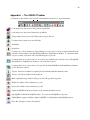
APPENDIX I -- THE SQUID-2 TOOLBAR ..........................................................................................................36
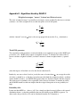
APPENDIX II: ALGORITHMS USED BY SQUID-2...........................................................................................37
WEIGHTED AVERAGES, “MEANS”, INTERNAL AND EXTERNAL ERRORS ....................................................................37
The MSWD parameter .......................................................................................................................................37
Probability of fit .................................................................................................................................................37
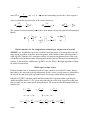
External errors and Weighted Averages assuming the presence of external errors ..........................................38
OUTLIER REJECTION FOR THE INTEGRATIONS COMPRISING A SINGLE SCAN OF A PEAK ............................................39
WITHIN-SPOT ISOTOPE RATIOS .................................................................................................................................39
OUTLIERS OF WITHIN-SPOT INTERPOLATED RATIOS .................................................................................................41
THE TUKEY’S BIWEIGHT ALGORITHM......................................................................................................................42
WITHIN-SPOT, NUMERICALLY-EVALUATED TASK EQUATIONS ................................................................................43
OVERCOUNTS ON 204PB ............................................................................................................................................43
OUTLIER-RESISTANT LINEAR REGRESSION .............................................................................................................43
CONCORDIA AGES ...................................................................................................................................................43
CONVERTING TERA-WASSERBURG TO CONVENTIONAL-CONCORDIA SLOPE-INTERCEPT ........................................44
207
PB/206PB AGE-ERROR INCLUDING ERRORS IN DECAY CONSTANTS: .......................................................................44
208-CORRECTED AGES AND RATIOS .......................................................................................................................45
207-CORRECTED AGES AND RATIOS .......................................................................................................................46
APPENDIX III: THE SQUID-2 PANELS AND CONTROLS ..............................................................................52
PREFERENCES ..........................................................................................................................................................52
Show splash-screen at startup............................................................................................................................52
Retain nonessential rows of PD or XML files (file length permitting) ...............................................................52
Place data-reduction parameters in a separate worksheet ................................................................................53
Place auto-charts in a separate worksheet ........................................................................................................53
Attach Task sheet to reduced-data workbook.....................................................................................................53
Freeze header rows and spot name column .......................................................................................................53
207-corrected 208Pb/232Th ages ......................................................................................................................53
208-corrected Concordia-plot ratios and 207Pb/206Pb ages ..........................................................................53
Create concordia plots for U-Pb Age Standards (U-Pb only) ...........................................................................53
Always construct within-scan isotope ratio sheet ..............................................................................................53
Set Y-axis minimum on isotope-ratio plots to zero.............................................................................................53
Maximum permitted mass-difference between measured and true nuclide masses… ........................................53
Default folder for PD and XML files..................................................................................................................54
Rebuild Task Catalog file...................................................................................................................................54
Isotope Ratios of Common Pb (U/Pb geochron only) ........................................................................................54
Calculation of within-spot, scan-by-scan means................................................................................................56
U/Pb calibration constant ..................................................................................................................................56
CORRECT FOR SECULAR DRIFT..............................................................................................................................56
U-Pb Standards..................................................................................................................................................57
Task ....................................................................................................................................................................58
New PD file ........................................................................................................................................................58
Number of characters to show in Standard names.............................................................................................58
Pb/U or Pb/Th Age.............................................................................................................................................59
Index Isotope for common Pb ............................................................................................................................59
Normalize ion beams to SBM signal ..................................................................................................................59
Spot subsets for user parameters .......................................................................................................................59
Time window ......................................................................................................................................................59
Trim mass charts................................................................................................................................................60
iii
Task Editor.........................................................................................................................................................60
Preferences ........................................................................................................................................................60
Change subsets...................................................................................................................................................60
Change Time-window ........................................................................................................................................60
REDUCE GENERAL ISOTOPE DATA ..........................................................................................................................60
New PD ..............................................................................................................................................................60
Task ....................................................................................................................................................................61
Normalize to SBM signal ...................................................................................................................................61
Make trim-mass charts.......................................................................................................................................61
Spot subsets for user parameters .......................................................................................................................61
Process spots within Time Window?..................................................................................................................61
Change Subsets ..................................................................................................................................................61
Task Editor.........................................................................................................................................................61
Preferences ........................................................................................................................................................61
Change Time-window ........................................................................................................................................61
SAMPLE GROUPING .................................................................................................................................................62
Spot Names.........................................................................................................................................................62
# letters to show in Spot-names dropdown.........................................................................................................62
Disregard Case, Spaces, Dashes, Slashes… ......................................................................................................62
Extract coherent age group................................................................................................................................63
Sort samples by age............................................................................................................................................63
Group all spots together.....................................................................................................................................63
Type of U-Pb Age...............................................................................................................................................63
Grouping Criteria ..............................................................................................................................................63
Construct concordia plot for groups if possible.................................................................................................64
Correction for 204 overcounts on Standard.......................................................................................................64
Common Pb........................................................................................................................................................64
TIME WINDOW ........................................................................................................................................................65
Limits to specify with Standard spots.................................................................................................................65
Starting Name/Time ...........................................................................................................................................65
Ending Name/Time.............................................................................................................................................65
SUBSETS ..................................................................................................................................................................66
COPY OR RENAME A TASK.......................................................................................................................................67
Task name ..........................................................................................................................................................67
Task description .................................................................................................................................................67
Primary mineral.................................................................................................................................................67
TASK EDITOR ..........................................................................................................................................................68
U-Pb Geochronology .........................................................................................................................................68
Isotope Ratio ......................................................................................................................................................68
Existing Tasks ....................................................................................................................................................69
Edit/view a panel for the selected Task ..............................................................................................................69
Refresh Task Catalog .........................................................................................................................................69
OK ......................................................................................................................................................................69
Cancel ................................................................................................................................................................69
Constants............................................................................................................................................................69
Save....................................................................................................................................................................69
RUN TABLE .............................................................................................................................................................70
Ionic species.......................................................................................................................................................70
Clear ..................................................................................................................................................................70
Specify mass station numerically .......................................................................................................................70
bkrd ....................................................................................................................................................................70
ref pk ..................................................................................................................................................................70
cps col ................................................................................................................................................................70
Hide?..................................................................................................................................................................71
Periodic table of the elements ............................................................................................................................71
Next ....................................................................................................................................................................71
iv
Return.................................................................................................................................................................71
Cancel ................................................................................................................................................................71
Insert ..................................................................................................................................................................71
Delete .................................................................................................................................................................71
Clear one............................................................................................................................................................71
Clear all .............................................................................................................................................................71
THE ISOTOPE SELECTION SUB-PANEL ....................................................................................................................72
How many? ........................................................................................................................................................72
Charge................................................................................................................................................................72
Enter...................................................................................................................................................................72
Complete ............................................................................................................................................................72
ISOTOPE RATIOS ......................................................................................................................................................73
Ratios (from mass stations at left)......................................................................................................................73
Next ....................................................................................................................................................................73
Back ...................................................................................................................................................................73
Cancel ................................................................................................................................................................73
U-PB SPECIAL EQUATIONS ......................................................................................................................................74
Equation for 206Pb/238Uconst..........................................................................................................................75
Equation for 208Pb/232Th const. ......................................................................................................................75
232Th/238U equation ........................................................................................................................................75
Equation for ppm U............................................................................................................................................75
Next ....................................................................................................................................................................75
Back ...................................................................................................................................................................75
Return.................................................................................................................................................................75
Cancel ................................................................................................................................................................75
Help....................................................................................................................................................................75
Append constant.................................................................................................................................................75
Append LITERAL ratios.....................................................................................................................................75
Append INDEX of ratios ....................................................................................................................................75
GENERAL EQUATIONS .............................................................................................................................................76
Next/previous equation (spinner) .......................................................................................................................76
ST, SA, SC, LA, FO, NU, HI, AR........................................................................................................................76
AR #rows #cols...................................................................................................................................................76
Constants............................................................................................................................................................76
Append column-header reference ......................................................................................................................76
Append LITERAL equations/ratios ....................................................................................................................76
Next ....................................................................................................................................................................76
Back ...................................................................................................................................................................77
Return.................................................................................................................................................................77
Cancel ................................................................................................................................................................77
Delete (active equation) .....................................................................................................................................77
Insert (active equation) ......................................................................................................................................77
Clear Active .......................................................................................................................................................77
Clear All.............................................................................................................................................................77
Help....................................................................................................................................................................77
Column headers .................................................................................................................................................77
Axis scaling ........................................................................................................................................................77
Calculations .......................................................................................................................................................78
Back ...................................................................................................................................................................78
Return.................................................................................................................................................................78
Cancel ................................................................................................................................................................78
CONSTANTS .............................................................................................................................................................79
Edit.....................................................................................................................................................................79
Add new..............................................................................................................................................................79
Delete .................................................................................................................................................................79
Exit .....................................................................................................................................................................79
v
Append to Eqn 1.................................................................................................................................................79
EXAMPLE TASKS .....................................................................................................................................................80
Zircon.................................................................................................................................................................80
230
Th ages, insignificant 232Th ............................................................................................................................82
230
Th ages, insignificant 232Th ............................................................................................................................83
Simple Monazite.................................................................................................................................................84
APPENDIX IV: WEIGHTED AVERAGE ALGORITHM FOR U/PB AGE STANDARDS............................85
APPENDIX V: SOME USEFUL EXCEL AND ISOPLOT FUNCTIONS ..........................................................86
NATIVE EXCEL FUNCTIONS .....................................................................................................................................86
AVERAGE ..........................................................................................................................................................86
MEDIAN ............................................................................................................................................................86
STDEV................................................................................................................................................................86
LINEST...............................................................................................................................................................86
INTERCEPT.......................................................................................................................................................86
SLOPE................................................................................................................................................................86
MAX, MIN .........................................................................................................................................................87
ISOPLOT AND SQUID FUNCTIONS ...........................................................................................................................88
sqBiWeight .........................................................................................................................................................88
ChiSquare ..........................................................................................................................................................88
Concordia ..........................................................................................................................................................88
ConcordiaTW .....................................................................................................................................................88
DisEq68Age .......................................................................................................................................................89
DisEq75Age .......................................................................................................................................................89
DisEq75Ratio .....................................................................................................................................................89
DisEq76Ratio .....................................................................................................................................................89
DisEqPbPbAge...................................................................................................................................................89
Drnd ...................................................................................................................................................................89
ExternalSigma....................................................................................................................................................89
HalfLife ..............................................................................................................................................................90
InitU234U238 ....................................................................................................................................................90
La230, La232, La234, La235, La238.................................................................................................................90
Lambda ..............................................................................................................................................................90
Log10 .................................................................................................................................................................90
Mad ....................................................................................................................................................................90
MSWD ................................................................................................................................................................90
NukeMass ...........................................................................................................................................................90
Pb76 ...................................................................................................................................................................90
ProbFit...............................................................................................................................................................91
RobReg...............................................................................................................................................................91
SingleStagePbT ..................................................................................................................................................91
SingleStagePbR..................................................................................................................................................91
sqWtdAv .............................................................................................................................................................91
StudentsT............................................................................................................................................................91
Th230Age ...........................................................................................................................................................92
Th230AgeAndInitial ...........................................................................................................................................92
Th230U238AR ...................................................................................................................................................92
ThUfromPb86 ....................................................................................................................................................92
U234age.............................................................................................................................................................92
U234ageAndErr .................................................................................................................................................92
U234U238AR ....................................................................................................................................................92
Output:
The present-day 234U/238U activity ratio..........................................................................................92
YorkInter ............................................................................................................................................................92
YorkInterErr95...................................................................................................................................................93
vi
YorkMSWD ........................................................................................................................................................93
YorkProb ............................................................................................................................................................93
YorkSlope ...........................................................................................................................................................93
YorkSlopeErr95..................................................................................................................................................93
APPENDIX VI: USEFUL ISOPLOT TOOLS FOR SQUID .................................................................................94
APPENDIX VII: DEFINITIONS OF TERMS .......................................................................................................95
204 corrected .....................................................................................................................................................95
207 corrected .....................................................................................................................................................95
208 corrected .....................................................................................................................................................95
Array function or formula ..................................................................................................................................95
Common Pb........................................................................................................................................................95
Concordance ......................................................................................................................................................95
Concordia ..........................................................................................................................................................95
Concordia age....................................................................................................................................................95
Constants............................................................................................................................................................95
Discordance .......................................................................................................................................................95
Dropdown ..........................................................................................................................................................96
Error correlation................................................................................................................................................96
External error ....................................................................................................................................................96
Grouping ............................................................................................................................................................96
Internal error .....................................................................................................................................................96
Ionic species.......................................................................................................................................................96
Isoplot ................................................................................................................................................................96
m/e......................................................................................................................................................................96
MSWD ................................................................................................................................................................96
Normalizing equation.........................................................................................................................................97
Panel ..................................................................................................................................................................97
PD file ................................................................................................................................................................97
Probability of fit .................................................................................................................................................97
Radiogenic Pb ....................................................................................................................................................97
Range .................................................................................................................................................................97
Resistant (mean, regression…) ..........................................................................................................................97
Robust (mean, regression…) ..............................................................................................................................97
Sample sheet.......................................................................................................................................................97
SBM....................................................................................................................................................................97
Scan order..........................................................................................................................................................97
Single cell formula .............................................................................................................................................97
Spot ....................................................................................................................................................................98
Stacey-Kramers..................................................................................................................................................98
Standard sheet....................................................................................................................................................98
Trim mass reference...........................................................................................................................................98
REFERENCES ..........................................................................................................................................................99
INDEX ......................................................................................................................................................................100
INDEX ......................................................................................................................................................................100
2
Introduction
Purpose of SQUID-2
SQUID-2.5 processes PD and XML files produced by a SHRIMP (Sensitive High Resolution Ion
Microprobe) into a variety of parameters, including raw isotope ratios, radiogenic Pb isotope ratios, ages for the U-Th-Pb system. The processed data can be applied to a broad range of run tables and applications, ranging from U-Th-Pb geochronology, 230Th/U geochronology, light stable-isotope geochemistry, and cosmochemistry. Processed data is placed in an Excel workbook
that, for most output parameters, makes the formulae used in each data processing step explicitly
available to the user.
Requirements
Software
SQUID-2 was developed using Excel 2003 (service pack 3) and Windows XP (service pack 2).
Earlier versions of Excel and other versions of Windows are probably compatible, but have not
been tested. SQUID-2 requires the Isoplot add-in (ver. 3.7 or later). Only English versions of
Windows and Excel are compatible with SQUID-2 and Isoplot.
ISOPLOT is BGC’s Visual Basic Add-in for Microsoft’s Excel® for data analysis and graphical presentation of geochronology, earth science and other radiogenic isotope data only.
BGC’s ISOPLOT is not the Isoplot® for analysis of any measuring system as described at
(http://www.shainin.com/ ). BGC is not affiliated with Red X Holdings, LC. Isoplot® is a
registered trademark of Red X Holdings, and is licensed to Shainin LLC.
At present, SQUID is not compatible with Excel 2007.
Hardware
WINDOWS
A mid- or high-range CPU (>1 Ghz non-Celeron, dual-core preferred) and 2 Gb or more RAM
is recommended. The screen resolution should be at least 1280x800.
EMULATED WINDOWS UNDER MACINTOSH OS-X
At least two of the several programs enabling running of Windows on an Intel Mac, at least two
– Parallels and Fusion – seem to work very well, with virtually no speed penalty compared to
Windows. Crossover cannot run Isoplot or SQUID.
Before installing SQUID on your Mac, please ensure that your screen resolution is adequate. For
wide-screen desktops, set your screen resolution from Windows (right-click anywhere on the
desktop, select Properties/Settings) to about 1920x1200. For laptops or smaller desktop screens,
use 1440x830 if possible.
3
Printer Setup
Upon first installation of Excel, a printer must be selected (via Page/Setup) before running
SQUID-2 or Isoplot, and the page size must be set to Letter or A4.
Input Data Files
SQUID-2.5 only processes PD or XML files for a single ion-counting collector.
Installation
1. If you’re running Windows from an Intel Mac under Fusion (Parallels is incompatible), you
must set Windows screen resolution to somewhat higher than the default setting. Right-click
anywhere on the Windows desktop (not the Parallels or Fusion desktop) and select Properties, then Settings . If possible, set the resolution to either 1440 x 830 or 1920 x 1200 pixels
2. Remove or rename all existing SQUID and Isoplot add-in file on
your computer. Excel tends to copy add-in files to its own folders,
so you must to a complete search of your hard disks (including
Hidden and System files) to make sure that Excel will not screw
everything up by having multiple, incompatible copies of Isoplot
and SQUID loaded at the same time.
3. Start Excel 2003. If you find that Excel has automatically loaded
either Isoplot or SQUID, close Excel and go back to step 2.
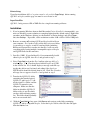
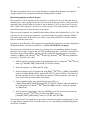
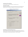
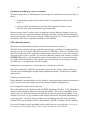
4. Select Tools/Add-ins from the Excel toolbar at the top of Excel’s
window (Figs. 1, 2). Check any boxes labeled Isoplot or SQUID
in the Add-ins list. Excel should display a message each time saying that the add-in can’t be found, and asking if the Isoplot or
SQUID add-in should be deleted from its list. Click Yes. If such a
message does not appear. close Excel and go back to step 2.
5. Transfer the SQUID-2.5 folder
containing the matched pair of
SQUID-2.5 and Isoplot 3.7 addins the SquidUser folder, and the
SQUID-2.5 manual to your
computer. Make sure that the
folder in which the SQUID-2.5
folder resides is one for which
you have full read/write permission. This folder should probably
not be on a network drive.
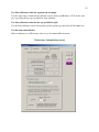
6.
Figure 1
Figure 2
With the Tools/Add-ins box open, click Browse and navigate to the folder containing
SQUID-2.5 and its compatible Isoplot. Select the Isoplot add-in, click OK, then OK again
from the Add-ins box.
4
7. Repeat Step 6, but this time select the SQUID-2.5 add-in. SQUID-2.5’s splash screen
should appear if installation was successful.
8. Before trying out SQUID-2, close, then re-open Excel. The compatible pair of SQUID-2.5
and Isoplot should now load automatically whenever Excel is opened.
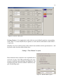
Data Reduction for U-Pb Geochronology
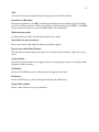
Click
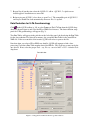
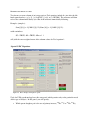
in the SQUID toolbar (p. 36) or select Process a Pb-U-Th Run from the SQUID dropdown list, then navigate to and select the PD or XML file of interest. The data-reduction setup
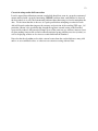
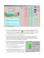
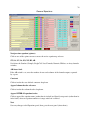
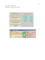
panel for U-Pb geochronology will appear (Fig. 3).
Two Run Tables will appear in the pink box at the left of the panel, the first being the Run Table
for the data-reduction Task already in memory, the second the Run Table for the actual PD or
XML file. If the two run tables don’t match, SQUID will refuse to process the file.
Note that when you select a PD or XML raw-datafile, SQUID will attempt to find a dataprocessing Task whose Run Table matches that of the PD file. This Task may or may not be the
one desired. If not, select the proper Task – say, Zircon, canonical ANU +UO2 – from the Task
dropdown.
Run table box
Figure 3: Setup panel for U-Pb Geochronology data reduction.
5
U-Pb/Th-Pb Standards
Specifying standards when starting data reduction
SQUID requires a 206Pb/238U or 208Pb/232Th standard to be among the analyzed spots in the PD
file. A standard for U or Th concentration is optional, and can be either the same or different
from the age standard. To specify a standard from the U-Pb data-reduction panel,
1. Select the number of initial characters to characterize the age–standard spots (e.g. 4 for
Standard spots with names such as SL13-1.1, SL13-2.1, SL13-3.1…), then select the
name of the age standard from the spot-name fragment dropdown.
2. Enter the 206Pb/238U (or 208Pb/232Th) age of the Age Standard. Enter the Age Standard’s
(apparent) 207Pb/206Pb age only if different from its Pb/U or Th/U age.
3. Select the U or Th concentration standard (if any) and enter its U or Th concentration.
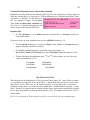
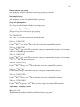
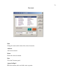
The Common U-Pb Standards List
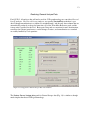
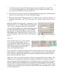
You can specify up to 50 common U-Pb age and/or concentration standards from the Preferences
panel (p. 57). When the U-Pb data-reduction panel is being filled out, SQUID will look for spot
names whose first few characters match those of an age standard. If a match is found, that standard’s name, Pb/U age (if defined), Pb/Pb age (if defined), and U or Th concentration (if defined) will entered into the appropriate boxes.
Figure 4: The U-Pb Standards page of the Preferences panel.
6
Specifying the common-Pb index isotope (U-Pb geochron panel)
204
Select Pb, 207Pb, or 208Pb from the Index isotope… dropdown (common-Pb isotope ratios are
specified in the Preferences panel; p. 52). The use of common Pb index isotopes is discussed in
pages 46, 63, 44, and 95)
Figure 5: Selecting the index isotope for
correction of common Pb.
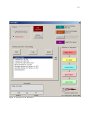
SBM Normalization
Indicate whether or not the secondary ion beam (pp. 34 , 59, 61, 96, 97) is to be normalized to
the SBM (secondary beam-monitor).
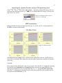
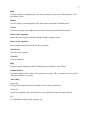
Trim Mass Charts
Figure 6: Trim-mass charts.
If the Make trim-mass graphics box is checked when starting data reduction, SQUID will contruct scan-by-scan charts of the trim masses for each of the centered mass stations (for Standard
spots only).
Click OK.
Data reduction will typically take a few tens of seconds, and yield an Excel workbook containing
not only the usual StandardData and SampleData sheets, but also the original PD data, condensed and reformatted for ease of examination (Fig. 8, p. 7). An optional Within-Spot Ratios
sheet (Fig. 7), containing the calculated scan-by-scan isotope ratios for each spot-burn can also
be requested (from Preferences; p. 52).
7
Figure 7: Fragment of an optional within-spot isotope ratios/sheet.
Condensed raw-data sheets produced by SQUID
When accessing a SHRIMP raw-data file SQUID first parses the PD or XML file, then converts
it into a formatted, space-efficient and user-friendly format.
XML files:
•
Can take as much as a minute to load and parse,
•
Can only yield a “Short” condensed raw-data sheet (see below) If the XML file
contains more than about 65,000 lines,
•
Contain extra information such as primary beam current, stage position, and
Qt1y-Qt1z settings, all of which can be plotted versus time as Autocharts (p. 30).
•
Can easily accommodate future additions to existing data parameters.
PD files:
•
Load and parse rapidly,
•
Can always produce “Long” (see below) condensed raw-data sheets if desired.
From the Preferences panel (p. 52), you can specify whether or not the condensed sheet should
retain the unformatted raw data in the first column of the condensed sheet (hidden by default),
thus automatically archiving the original PD or XML file. Such auto-archiving slows down dataprocessing slightly, so if these files are normally archived elsewhere, is not recommended.
Auto-archived condensed sheets are identified as PD file, Long rather than PD file, Short (for a
PD file) in the top row of the condensed sheet (Fig. 8).
Figure 8: PD file after condensation and reformatting by SQUID.
8
Reduced-data sheets produced by SQUID
The StandardData Sheet
The Standard sheet contains processed data for only the
Age Standard spots. Among the changes from SQUID-1
are:
•
Additional data-columns containing the results for
any Task equations (e.g. the Log UO/U and Log
Pb/U columns in the example at right; p. 20).
•
Up to eight user-specified, Task-linked plot insets,
(e.g. Log UO/U versus Log Pb/U) each linked to
one or two of the data columns (p. 30).
•
A minimum Pb/U external error can be assigned to
the Age Standard in the Preferences panel (p. 52).1
•
Automatically-generated Concordia plots for
the Age-Standard data can be requested (p.
53).
•
A correction can be applied for obvious secular drift of the Standard calibration-constant
(p.10).
Figure 9: Portion of StandardData worksheet showing
the U/Pb calibration columns.
CORRECTION FOR OVERCOUNTS ON 204PB
SQUID will attempt to quantitatively assess the presence of nonPb counts at the 204Pb mass position by 1) assuming precise concordance of the 206Pb/238U-207Pb/235U ages, and also 2) assuming
precise concordance of the 206Pb/238U-208Pb/232Th ages. The (resistant) mean value of the calculated 204-overcounts on the age-
204
Figure 10: Column headers for
204 overcounts on the U-Pb age
standard.
1
Assigning a reasonable external error, based on an experienced operator’s judgment from past data-sets, is important if the age standard has low enough count-rates that the counting statistics errors mask a (smaller) external variance. In such a case, if the sample spots have a significantly higher count rate, so that the external error is comparable to or greater than their counting-statistics errors, the errors assigned by SQUID to the sample spots will be underestimated, so that even well-behaved, age-equivalent spots will not yield a statistically coherent Group.
9
standard spots can then, if desired, be used to correct 204Pb measurements for all of the Sample
spots when the samples are Grouped (p.9). The output-columns related to calculation or 204
overcounts are shown in Fig. 10.
The SampleData Sheet
As in SQUID-1, the Sample sheet contains the basic raw and processed data for all spots but
those of the Age Standard. For U-Pb geochronology, the Sample Sheet is to be used only as an
intermediate step in producing the final, Grouped Sample worksheets.
Sample Grouping and Age Extraction
`Data reduction for U-Pb geochronology is not complete until the sample–spot data has been
grouped by spot name. Group names are selected from one or more of six drop-down lists containing all Spot names, trimmed to the number of initial characters shown in # of characters
spinner-box (red arrow, fig. 11). The dropdown lists will not show spot-name fragments unless
at least 2 spots are thus defined.
To Group samples,
Figure 11: The Sample Grouping panel.
10
•
Click
in the SQUID toolbar, or press the Group Me button at the top of the SampleData sheet.
•
Select the number of initial spot-name characters to define a Group (red arrow, below),
•
Indicate whether case is significant in the name fragments, and whether or not to ignore
spaces, dashes, slashes … when identifying name-fragment matches,
•
Specify from 1 to 6 spot-name groups,
•
Indicate if a statistically-coherent age group is to be extracted from each spot-name
group.
•
If age grouping is requested, then
•
Indicate whether the data-rows in each grouped-sample worksheet should be
sorted by spot age,
•
Specify the type of age to use for age grouping, the criteria that define an age
group, and whether to construct a concordia-plot inset for the spot group,
•
Specify the method of correction, if any, for 204Pb overcounts (No correction is
recommended unless you have a good understanding of the concept),
•
Define the common-Pb ratios for the groups.
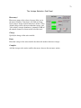
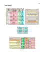
Correcting U-Pb Geochronology data for Secular Drift of Age-Standard Spots
Normally, the calibration constant (e.g.
Pb+/U+ ÷ UO+/O+) measured for the different Pb/U or Pb/Th age-standard is expected
to remain, within some statistical scatter,
constant during the length of the analytical
session, so that extracting the true Pb/U or
Pb/Th ratios of samples is a simple matter
of normalizing the sample calibration constant to the average value of the Standard
spots. If, however, the analyst can plainly
Figure 12: Setting parameters for correction of secular
see a trend in the Standard calibration condrift of the U/Pb calibration constant. (Preferences panel).
stants (whether monotonic or cyclic), it is
possible that the Sample spots will have been similarly affected. SQUID-2 provides a very flexible, tuneable, assumption-independent method for dealing with such cases, enabled by checking
the secular drift box (right) in the Preferences/Interpolation panel (p. 52).
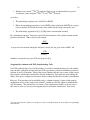
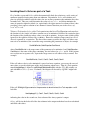
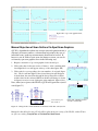
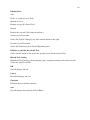
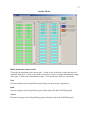
If the user has selected Specified, the secular drift correction algorithm starts by fitting an outlier-resistant smoothed-spline curve (a LOWESS fit; Cleveland, 1979) to the Standard calibration
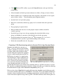
constants, using a moving window for smoothing comprising the specified number of spots. Instead of the usual weighted-average chart, SQUID-2 will then construct a chart showing the rela-
11
tive change of the calibration constant versus spot-time, and the corresponding smoothedspline curve.
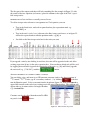
8 0.00%
12 0.78%
16 0.79%
36 0.81%
Figure 13: Showing the effect of different smoothing-window widths (yellow boxes, in number of spots)
on the secular drift curve of the Age Standard calibration constant relative to its median value (red line).
Estimated external (non-counting statistics) error is shown in the blue boxes. Small red circles indicate the
Age standard calibration constant, black vertical lines their 2σ internal errors.
If, however, the user has selected Automatic for the smoothing window, SQUID-2 will automatically find the largest smoothing-window that yields an external scatter no greater than the assigned Minimum acceptable external error for the age Standard.(p. 57). The Min. spots parameter (p.
12) sets the lower bound on the automatic smoothing-window.
The secular drift of Age Standard’s calibration constant (relative to the median value) is then
used to correct the calibration constants of the Standard spots (i.e. to remove the presumed effects of the Standard’s drift).
Note that secular-drift correction will only be applied for Tasks with a single parent-daughter
system (Pb/U or Pb/Th) specifically calculated (that is, where calculation of the non-Primary
parent-daughter ratio is specified as Indirectly in the U-Pb Special Equations panel (p. 27).
12
Caveats in using secular drift correction
It can be argued that calibration-constant secular drift should not occur in a properly constructed
mount analyzed with a properly functioning SHRIMP, and that when such behavior is observed
the best remedy is to solve the instrumental problem rather than trying to cleverly manipulate the
data. To the extent that this is the case, it is quite possible that attempting to correct for such
drift will degrade rather than improve the accuracy and precision of the resulting U/Pb ages. Of
particular concern is the possibility that, though the apparent external scatter of the Standard
spots mad be reduced, drift-corrected Sample spots of the same true age will have increased scatter (thus making it impossible to find a coherent statistical group without excessive rejection), as
well as displaying an more-or-less inverse secular drift from the Standard.
Note also that the algorithm used to infer external scatter from the secular-drift curve may yield
under- or over-estimated values, as it has not seen extensive testing with real data.
13
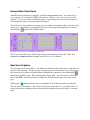
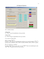
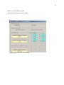
Reducing General Isotope Data
For SQUID-2, all analyses that will not be used for U-Pb geochronology are considered General
Isotope analyses. For General Isotope analyses, no separate StandardData worksheet is produced (though normalization to a standard is straightforward), and the only data columns that are
automatically produced are those for burn time, cps of the Trim-Mass Reference peak, and the
isotope ratios specified for the Task. Basic processing such as correction for mass fractionation,
correction for isobaric interferences, secular changes in ratios, and normalization to a standard
are readily handled by Task equations.
PD file (click to change)
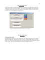
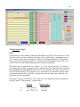
Figure 14: Setup panel for General Isotope Ratio data reduction.
The Reduce General Isotope data panel for General Isotope data (Fig. 14) is similar to, though
much simpler than that of U/Pb geochronology.
14
Tasks
Introduction
Tasks are the templates used by SQUID-2 to process the raw PD files. Each Task contains the
algorithms by which the data is processed into final isotope ratios, ages, element concentrations,
and any other parameter of interest to the user.
The gateway into defining, viewing, and editing Tasks is the Task Editor panel (Fig. 13 – press
on the SQUID-2 toolbar). There are two classes of Tasks: U-Pb Geochronology and Isotope Ratio. The former is specifically constructed for processing analyses on minerals such as
zircon into a complete set of relevant total and radiogenic isotope ratios, together with their associated ages. The latter is for any other type of analysis.
Each SQUID-2 Task is defined by an Excel workbook (*.xls) file contained by the SquidUser
folder, located in the same folder as the SQUID-2 add-in file. Names of Task files always begin
with SquidTask_ , followed by the name of the Task and name or initials of the Task’s creator.
Existing Tasks defined in the default SquidTasks file are shown in the scrollbox at the lower left
of the panel. After you create any additional Tasks of your own, all of your interactions with the
Task editor will be to modify existing Tasks via one or more of the Edit/view buttons.
Task definition is a four or five step process (General Isotope and U-Pb geochron data, respectively), in which you will:
1. Define mass stations for the PD file’s Run Table,
2. Specify isotope ratios to be calculated from the Run Table,
3. Define equations for calculation of U/Pb (or Th/Pb) and 232Th/238U ratios and for U (or
Th) concentration (U-Pb geochron only),
4. Define equations for any additional data-processing, and
5. Specify chart insets for x-y plots, means, or secular trends of any of the final data columns.
The best way of to get an idea of what a Task consists of is to go through the process of creating
one from scratch, using, for example, the canonical (ANU-RSES) run table and equations.
15
Figure 15: First panel of the Task Editor.
16
The Task Name Panel
Each Task is assigned a unique name (Figure 16) – preferably a reasonably pithy one that fits
within the Task list-box of the Task Editor. The Task Description should contain additional information about the purpose of the Task and type of data required. The Primary Mineral and
Creator name of initials fields are self explanatory.
CanonicalZirconPlus270
UO2 peak included to test for odd spatial effects, as well as alternate U/Pb calculation
zircon and baddelyite
Alistair Schnuckf III
Figure 16: The Task name, description, mineral, and creator panel.
The Run Table Panel
Defining the Run Table
From the Existing Tasks list of the Task Editor (Fig. 15), click the New button, thus invoking a
blank Run Table panel. For illustration, figure 17 shows a completed Run Table panel (for UPb/zircon) , but of course when defining a new Task, all of the entries in the right-hand scrollbox
will be empty. The steps for definition of the canonical zircon Run Table are:
17
Figure 17: The Run Table panel.
1. Set the active Ionic Species or numeric mass box (the one in the right half of the panel) to
control. The active Ionic Species… box is tan
Scan Order 1, using either the mouse or the
rather than pink, as for the Ionic species box for scan order 10 in the example panel (figure
17). We now wish to enter 90Zr216O+ for the first mass position in the run table.
2. Click on the zirconium (Zr) box in the periodic table.
The resulting isotope selection dropdown (figure 18) will show all of the stable and longlived isotopes of the element, with the most abundant selected by default (relative abundances are shown to the left of the isotopes). In this case, the default of 90Zr is fine (to select
any other Zr isotope click on one of the black isotope boxes).
3. Select the number of atoms of this isotope in the ionic species (using the How Many spin-box), then click
OK. 90Zr2 + will appear in the active Ionic Species
box in the right half of the panel.
4. We know that the final nuclide will have a charge of
+1, so we can leave the Charge box as it is.
5. Click the Enter button, which will dismiss the Select
Isotope panel, then click on the yellow O(xygen) box
in the periodic table. Select 16O, quantity 1, charge
Figure 18: The Select isotope box.
18
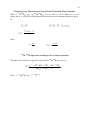
1. Click the Complete button. The nuclide (ionic species) box should now contain 90Zr2
16
O + ref in the Ionic species box, with 195.804 as its mass to charge ratio, and the active
ionic species box should move down one in the list.
6. Check the small ref pk box to the left of the Ionic species box (figure 20) so that this nuclide
will be used as the reference mass for any Trim Mass graphics
7. Enter the singly-charged 204Pb ion as the next (scan order 2) ionic species/mass station by selecting Pb as the element, and 204Pb as the isotope. Click Complete again to move to scan order 3.
In PD files that this Task will process, scan number 3 is the
background mass of, say, 204.09. Because the background
“mass” doesn’t correspond to that of any actual nuclide,
you must click the Specify mass station numerically button
(just above the periodic table; figure 17), type in 204.09,
then click OK. Now check the Bkrd box to the left of the
Ionic species box to indicate that this mass station is to be
used for background. Move on to the next mass station as
before.
Specify mass station numerically
Figure 19: The Specify mass numerically
box.
And so on.
Note that if the ionic species you are defining
is, say, doubly or triply charged, you can
specify the charge with the spin-button to the
right of the box you used to enter the numeric
mass. The mass/charge ratio of the ionic
species will automatically adjust.
Figure 20: Completed entry for scan order #1.
If you want to have a column containing the (total) counts/second of a mass station placed on the
output worksheets, check the corresponding cps col box to the left of the ref pk box (figure 20).
Cps col boxes are automatically checked for reference and background mass-stations, and also
for the 204Pb and 206Pb mass stations.
When you’re done, look at the Nominal mass column to the right of the True mass column. The
Nominal masses are usually (but not always) an integer, but SQUID-2, if necessary, will have
added just enough additional decimal places to distinguish the masses of each mass station from
the other. Thus true mass of 204.09 that you entered for the background mass-position will be
shown as 204.1 to distinguish it from the nominal 204 assigned to the 204Pb+ mass station. When
referring to the isotope ratios or mass positions of the Run Table in the Equations panels, always
use these nominal masses.
19
Specifying Isotope Ratios
The next step is to specify which isotope ratios should be calculated. The order of the ratios will
be preserved in the output worksheets, but otherwise is unimportant. To enter a ratio,
•
Click on a blue ratio-box (figure 21) to activate it (its color will change from blue to orange
when activated),
•
Click on one of the nominal masses in the green boxes to the left (say 204) to use as the numerator of the ratio,
•
Click on another of the green boxes to select the denominator isotope (say 206), giving
204/206 in the ratio box, whose color will have changed back to blue.
•
To clear the ratio box and start over, click it a third time.
•
The ratio boxes don’t have to be all filled in sequence – empty boxes are ignored.
Figure 21: The Isotope Ratios panel.
20
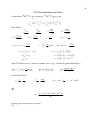
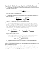
Figure 22: The General Equations Task panel.
The Equation Panels
Basics
Task equations are the backbone of the built-in flexibility of SQUID-2. The variables in a Task
Equation can be any of the worksheet cells in the processed-data sheet(s), including isotope ratios, and the results of other Task equations. There are two Equation panels for U-Pb geochronology, and one for General Isotope data. I will discuss the General Equations panel first, as it
exists in Tasks for both U-Pb/geochronology and General Isotope Ratios.
The simplest type of equation have no “switches” (p. 23) set, and use only the Tas’s isotope ratios and numeric constants as arguments for the algebraic functions. Equation results are placed
in the SampleData or StandardData output sheets, in data columns to the right of all of the isotope-ratio output columns. If no switches are set, uncertainties for each of the equation results
are calculated numerically by SQUID-2, with all of the relevant isotope-ratio errors and error
correlations correctly propagated.
For example, consider a U-Pb/zircon Task that has two User Equations defined (in addition to
the four “special” U-Pb equations), as shown above.
Equation
Equation Name
(1)
Ln([“254/238”])
Log UO/U
(2)
Ln([“206Pb/238U”])
Log Pb/U
21
The first part of the output worksheet will look something like the example in Figure 23, with
the results of the two equations (red arrows) placed in columns to the right of the Task’s specified isotope ratios.
REFERENCING AN ISOTOPE RATIO IN THE EQUATIONS PANEL:
To add an isotope-ratio reference as an argument in a Task equation, you can:
•
Type in the literal ratio, enclosed in square brackets plus a quotation mark, e.g.
[“207/206”], or
•
Type in the ratio’s index letter (adjacent to the blue isotope-ratio boxes, as in figure 22,
enclosed in square brackets without quotation marks, e.g. [b], or
•
Just click on the blue isotope-ratio box for the ratio you want.
Figure 23 A reduced zircon SampleData worksheet for a Task having two user-defined equations (red arrows).
If you append a ratio by just clicking its ratio box, the ratio will be appended to the end of the
existing expression (if any) in the active equation-box. You can choose which style will be used
by toggling between Index (appends the letter-index of the ratio, e.g. [h]) and Literal (appends
the ratio itself, e.g. [“238/196”]) with the
button.
ADDING A REFERENCE TO A NAMED NUMERIC CONSTANT:
You can define, view, and insert up to 250 constants constants (such as the decay constant of
U, natural 238U/235U ratio, age of a secondary standard…) by clicking
at the bottom the Equation panel. Select a constant from the dropdown (figure 24), then click Append to
append the constant to the end of any existing text in the active Equation box. The constant will
appear either as its name enclosed in angled brackets,
e.g. <Lambda238>.
238
Constants can also be edited from the main Task Editor panel, via the
button..
Figure 24: The Constants dropdown.
22
Named numeric constants are stored both in the User Preferences workbook and with the Task
itself. If a conflict in the values stored for a named Task is detected when the Task is loaded, you
will be prompted to resolve the conflict, and the selected value will be made consistent in both of
the stored locations.
ADDING A REFERENCE TO OTHER TASK EQUATIONS:
Any equation can use the results of any other equation as an argument. To do this, you can
1. Type in the name of the equation (see below), enclosed in square brackets plus a quotation mark, e.g. [“Log UO/U”]. Case, spaces, and slashes (/) are ignored by SQUID, so
you don’t have to type them in when defining an equation.
2. Type in the equation’s index number (in the orange equation# box to the left of the equation box itself), enclosed in square brackets without quotation marks, e.g. [13], or
3. Just click the equation-number box to the left of the equation box.
Unless you use the FO switch (see below), you should make only forward references to other
equations – that is, to higher-numbered equations – so that the results of the equation referred to
will have been calculated when needed.
EQUATION NAMES:
Each Task equation must be assigned a name in the corresponding Equation Name box (figure
20). The equation name will be used as the column header for the equation’s output column the
SampleData or StandardData worksheet and, if the equation’s SC switch is set, as an Excel
range name2. To avoid overly-wide columns for the equation results, you can use the | character
to indicate a linefeed. Thus an equation name entered as
Mean rad.|ppm Pb|(uncorr.)
would appear in the equation’s column header as:
For Array Equations (see p. 25) whose output occupies more than a single column, you can specify names for each of the output columns using a double vertical-line (||) as the columndelimiter. Thus the output for a name such as
2
SQUID will ignore non-alphanumeric characters (underscore excepted) in SC equation names, as only alphanumeric characters are permitted in Excel range names. Initial number-characters are also forbidden.
23
Th230|raw age|(ka)||err||Init|234/238||err
assigned to the array equation
Th230AgeAndInitial([3],[±e],[1],[±f], ,true)
with the ARrc switch marked as 14 (output occupies 1 row, 4 columns) would be something like:
EQUATION Switches
To provide more control over how and when the Task Equations are evaluated, SQUID-2 provides up to 7 “switches” that can be turned on or off for each equation. The Switches and their
abbreviations are (shown in blue font if restricted to U-Pb/geochron):
Switch
Function
Standard
The equation is placed only in the Standard output sheet (default is both).
SAmple
The equation is placed only in the Sample output sheet (default is both).
Single Cell
The equation results occupy a Single Cell rather than a column, and operates on whole columns of data rather than the data in just one row.
LAst
The equation is to be calculated last, after all of the other equations without the LA switch, and after all of the columns produced automatically
(e.g. radiogenic isotope ratios, U concentration, apparent ages…) by
SQUID-2.
The column-order of calculation for U-Pb geochronology is:
•
Isotope ratios as specified in the Task.
•
Task equations for which neither the SC nor LA switches are
set.
•
Automatically calculated columns (radiogenic isotope ratios, U
concentration, apparent ages…).
•
Task equations whose SC, but not LA switch is set.
• Task equations with the LA switch set.
The order of calculation within each category follows the equation
index-number.
24
FOrmula
The Formula for the Excel equation is to be placed in the output cell(s),
rather than its numeric result.
NUmeric
The Numeric value of the Excel formula for the equation is to be placed in
the output cell(s), rather than its Excel formula.
HIdden
The worksheet column containing the Equation results will be hidden.
ARray formula The equation is an Excel Array Formula whose output can occupy more
than one row and/or column.
ARrc
The number of rows and columns occupied by the output of the array formula (two numbers separated by a space).
The ST and SA switches (U-Pb/geochron): When examining and calculating data that is relevant
to, say, just the age-standard spots, the output of user equations that have been created for this
purpose (say to examine the Log(Pb/U) vs. Log(UO/U) slope) would only clutter up the Sample
output sheet. With the ST switch on, the column headers and output for such equations will be
calculated and placed only on the Standard sheet. Conversely, the SA switch restricts the equation to the Sample worksheet. If neither of these switches is on, the equation is placed on both
sheets.
The SC switch (U-Pb/geochron): This switch specifies an equation that operates on whole columns of data, using Excel functions such as Average, Median, STDEV…, and Isoplot or SQUID
functions such as BiWt, RobReg, AgePb76, Th230age, InitU234238….. An SC-switched equation is placed in only one cell (rather than each cell in a data column). Thus if interested in, say,
the median of the measured 204/206 ratios, one would create an equation with the formula
Median([“204/206”]
The LA switch (U-Pb/geochron): If a cell reference in a (numerically evaluated) User Equation
hasn’t been calculated and placed on the output sheet, the output cell of the equation will either
incorrect or an Excel error. Unless the Equation’s SC switch is on, data for isotope ratios and
lower-numbered equations will always exist. However, the radiogenic-isotope and age-columns
created by SQUID-2 are placed on the output sheet after all equations, except for those equations whose LA switch is on.
The FO and NU switches: SQUID puts the results of its calculations in the output-sheets cells as
either the numeric value of the calculation (e.g. 1.234) or as an Excel formula (e.g.
=$C13/$F13-SQRT($AE13-$AF13)*[“ppmu”] ). Advantages of a NUmeric result are:
•
Quickest start-to-finish data- processing,
•
Least “fragile” output sheets, in that the equation-result cells are invulnerable to changes
or errors in the source cells arising from later changes to the worksheet,
•
Automatically-calculated errors are (if the equation references only isotope-ratio columns) rigorously accurate, and placed in the column to the right of the equation column.
25
Advantages of a FOrmulaic result are:
•
The equation’s output cells are updated automatically when changes are made to
cells referenced by the equation,
•
Other equations on whose results are referenced by an FO equation need not have
been calculated before the FO equation.
•
The user can check the contents of the equation cells to make sure that the equation actually implements the user’s intent.
The H switch: If set, this switch causes the column containing the Equation’s results to
be hidden (useful if the output worksheet is too cluttered with non-essential information).
To unhide a hidden column, select the two columns flanking the hidden column, then unhide with Format/Column/Unhide. To unhide all hidden columns in a worksheet, select
all cells by clicking on the blank rectangle at the interestion of the Row and Column indices.
The AR switch: This switch, which requires some knowledge of Excel’s Array functions, adds
another level of flexibility in data processing. You will have to use the Excel documentation to
learn the general ins and outs of Array Functions, but an important feature is that the output of
these functions can occupy not just one cell, but any group of contiguous cells with an arbitrary
number of rows and columns. For example, the complete output of the Isoplot array function,
230ThAgeAndError()
occupies (up to) 5 contiguous cells in the same row, comprising
Age, age±, initial 234U/238UAR, initial±, age-initial error correlation
Other array functions may occupy, say, a 2-column by 5-row range. You must therefore specify
the number of rows and columns in the output sheets that SQUID-2 will need to reserve. To do
this, enter first the number of rows (1 to 9), then the number of columns(1 to 9) in one of the
Equation panel’s AR #rows #cols boxes, without spaces or commas – for example, as 24 to indicate a 2 row by 4 column output range.
If the array function’s output range occupies both multiple rows and multiple columns, the output cells can be referred to by other equations by their assigned name plus the characters for the
#rows and #columns. For example, the second row, first column of a 3-row by 2-column arrayfunction output named “ThAge” would be named “ThAge21”. See p. 22 regarding other naming conventions for Array equations.
If, for an Array equation, you specify fewer rows or columns than the maximum possible for the
equation (e.g. 2 rows, 1 column instead of the 3 rows by 2 columns that the Array function in the
equation’s can populate), only the that number of rows/columns will be occupied in SQUID-2’s
reduced-data worksheet.
26
The above description of how to use Array Functions is admittedly inadequate, but should be
enough to allow you to experiment until better documentation is written.
Restricting equations to subsets of spots
The operation of a Task equation can be restricted to a specific suite of spots that, like the Age
Standard spots, can be grouped by the first few characters of their spot names. Subset-restricted
equations can be defined either at the time of data reduction (p. 29) or as part of the Task equations. When a Task equation is restricted to a subset of spots, cells in the equation’s output column will be empty for all spots but those in the subset.
Subset-restricted equations are normally defined along with the data-reduction Task (p. 26). You
can, however, also restrict any equation to a spot subset at the time of data reduction, which is
convenient if the names of the subset spots tends to vary from one PD file to another. Instructions are within the panel itself.
Spot subsets are defined for a Task equation by appending the appropriate spot-name fragment to
the Equation Name, enclosed in curly braces, e.g. Mean 207Pb/206Pb rad. {qgng}.
Spot subsets are useful when you want to use certain spots as a normalizing standard for some
parameter. For example, suppose that, for U-Pb geochronology data, you wish to correct Pb isotope ratios for mass fractionation, and that you have included in the grain mount a secondary
standard, say RRhy, with a known 207Pb*/206Pb*(the Age Standard 207Pb/206Pb being insufficiently precise). To do this, one could:
1. Add an equation consisting simply of the SampleData sheet’s radiogenic 207Pb/206Pb column, e.g. [“4corr207*/206*”] with the SA, FO, and LA switches,
2. Name the equation, e.g. RRrhy rad 7/6 {rrhy} ,
3. Add an equation for the resistant mean of the RRhy 207Pb/206Pb, e.g. BiWt( [“rrhyrad7/6"] ,
named, say, Mean RRrhy rad7/6 , with the SA, SC, FO, and LA switches. Note that neither this equation nor the two that follow are marked as Subset equations, since they operate on all of the spot-data within each column.
4. Add an equation for the mass-fractionation factor for Pb, e.g.
[“Mean RRrhy rad7/6”]/0.10736 with the SA, FO, and LA switches, where the number in
the denominator is the known 207Pb/206Pb for the RRrhy standard. Name the equation,
say, MassFract ,
5. Add an equation (approximate, since the 204/206 is to be left uncorrected) for the fractionation-corrected 207Pb/206Pb of all of the non-RRrhy spots, e.g.
[“4corr207*/206*”]*[“MassFract”], named, say, Fract. corr. 207*/206* .
You can also restrict Task equations to spot subsets via the data-reduction startup panels (p. 26),
to avoid defining separate Tasks if only the names of, say, a normalizing standard change from
one PD file to another.
27
REFERENCING ERROR COLUMNS
To reference an error column of an isotope ratio or Task equation, include +– just after the lefthand square bracket, e.g. [+-3], [+-LogUO/U], [+ -b], or [+-207/206]. The reference will then
refer to the column immediately after that of the reference immediately following.
Example (complex):
Sum([1]/([+ -1]/100*[1])^2)/Sum(1/([+ -1]/100*[1])^2)
with switches
SC = TRUE, AR = TRUE, ARrc = 1 1
will yield the error-weighted mean of the column-values for Task equation 1.
“Special U-Pb” Equations
Figure 25: The U-Pb Special Equations panel.
Tasks for U-Pb geochronology have this extra panel, which pertains only to the particular needs
of this type of analysis. In this panel, you will specify:
•
Which parent-daughter pair is the one of primary interest (206Pb-238U or 208Pb-232Th),
28
•
Whether you want the 232Th/238U calculated directly, by an equation that you specify,
or indirectly, from calculated 206Pb/238U and 208Pb/232Th ratios,
As well as:
•
The normalizing equation to use for Pb/U (or Pb/Th),
•
Either the normalizing equation to use for Pb/Th (direct calculation of Pb/Th) or an equation to calculate Th/U from the isotope ratios defined in the isotope ratio panel, and
•
The normalizing equation for [U] (or [Th]) from a concentration standard.
By “normalizing equation” I mean an expression whose numeric value remains constant for the
parameter of interest. Thus in the present example,
Pb/U
(UO/U )2
is expected to be constant (during the analytical session) for any given value of Pb/U, and
U/Zr
(UO/U )0.66
should be constant for any given U/Zr (the proxy for [U]).
Swapping data columns with U-Pb Geochronology Tasks
For U-Pb geochronology data, SQUID produces several data-columns having to do with calibration constants, radiogenic-isotope ratios and U-Pb ages that are produced in addition to and independent of any Task equations. Most of these data columns reference one or more of the isotoperatio columns, which cannot normally be directly modified by Task equations, thus limiting the
ability of the user to compensate for factors such as isobaric interferences and mass fractionation.
However, Task equations can be modified using a “column swapping” feature, which permits
modification of any of the isotope ratio columns3, and thus most of the otherwise-unmodifiable
SQUID columns. The general idea is to create a Task equation that modifies (corrects) an isotope ratio in some way (say by correcting the ratio for an isobaric interference), then to add
3
The four “Special U-Pb” equations are exceptions, as they are calculated directly from the within-scan peak-height
measurements.
29
“<=>” to the equation directing SQUID to exchange the modified value with the original result.
For example, suppose there is an interference on 204Pb that is roughly proportional (say about
double) to the counts on mass 203. The correction can be made as follows:
1. Add the Task equation [“204/206”] – 2*[“203/206”] <=> [“204/206”],
2. Name the equation.
When done, the 204/206 column of output-data sheet will contain the raw (measured) 204/206
minus double the measured 203/206, and retain the original 204/206 column header, and the
Task equation’s column will contain the original (measured) 204/206, with the header RAW
204/206.
Referencing data in other workbooks or worksheets
For U-Pb Tasks, the same column header can exist in both the SampleData and StandardData
worksheets. SQUID will first look for the referenced column-header in the worksheet doing the
referencing, then (if not found) in the other (StandardData or \SampleData) worksheet.
To reference data in either another workbook or to override the above procedure, you must include the workbook and worksheet name using Excel’s syntax (required characters in red), e.g.
To refer to cell A1 in another workbook:
′[WorkbookName]SheetName′!RowColAddress
or
′[WorkbookName]SheetName′! RangeName
for example:
′[MonaziteStdData]CorrectionFactors′!B23
to reference cell B23 in the worksheet “CorrectionFactors”, contained in the workbook
“MonaziteStdData”.
To refer to cell A1 in another worksheet in the same workbook as the PD file being processed:
′SampleData′!A1
30
Viewing Task Equations in the reduced-data workbook
Equations associated with the data-reduction Task used for data reduction are always shown in
either the StandardSpots or SampleSpots (U-Pb geochronology or General Isotope Ratio Tasks,
respectively) worksheets via the Equations
Box (see example at right). If the Attach
Task sheet to reduced-data workbook box
in Preferences is checked, the equations will
also be shown in the attached Task sheet.
Equation Tips
•
Use the sqBiWeight (p. 88) or Median functions instead of Excel’s Average to avoid worrying about outliers.
If you need to use an error-weighted mean, use the sqWtdAv function (p. 91).
•
Use the RobReg function (p. 91) instead of Slope, Linest, Yorkfit, or Yorkslope functions,
again to eliminate sensitivity to outliers.
•
Use the Min and Max functions to restrict the range of an output, e.g.
Min(3, Max(1, Median([“CalibrSlope”])) to force CalibrSlope within the range of 1 and 3.
•
To deal with initial disequilibrium in the 238U or 235U decay chains, use one of the relevant Isoplot functions (p. 89),
DisEq68Age
DisEq68Ratio
DisEq75Age
DisEq75Ratio
DisEqPbPbAge
DisEq76Ratio
The Autocharts Panel
The final panel in the definition of a Task is for Auto Charts (figure 26). Auto Charts are simple
x-y or weighted average plots of any of SQUID-2 ’s output sheets that are placed as insets in the
these sheets. Up to 8 Autocharts (p. 30) can be requested. You can choose the x and (if not a
weighted average plot) y axes from any of the output sheet’s column-headers using the x-y dropdown. You may also request that an (outlier resistant) linear regression be calculated and plotted
for x-y data, or an (outlier resistant) mean for just the y data. If Y mean is selected, the x axis is
always Hours.
For U-Pb geochronology Tasks, Autocharts will be created only for the age-standard spots.
31
Figure 26: The Auto Charts panel.
In figure 26 (above), for example, the results of the two (user-defined) equations corresponding
to Ln(206Pb/238U) versus Ln(254/238) are plotted, as well as the line and numeric results of the xy regression.
Normally, Autocharts will be placed on the reduced-data worksheet of the spots themselves. will
be placed on the Standards reduced-data sheet
Setting a “Time Window” for spots
Data reduction can be restricted to any sequentially-measured series of spots. For U-Pb geochronology, the series
of spots is defined by the bracketing Age-Standards. For
General Isotope data, the time window is defined by any
pair of bracketing spots.
Figure 27: The Time Window panel.
32
Specifying Subset-restricted equations at the time of Data Reduction
A “subset-restricted equation” is a user-defined Task equation that will operate only on a subset
of the spots in the PD file, where the subset is defined by the initial characters of the spot names.
This can be very useful, for example if one wishes to know the mean U concentration of just
those spots whose names start with “MG”.
Subsets can be assigned either by the data-reduction Task (p. 37) or at the time of data reduction
by clicking the Subsets button on the data-reduction panel.
Figure 28: The Subset panel for specifying subset equations at the time of data
reduction.
33
Invoking Excel’s Solver as part of a Task
Excel includes a powerful Solver add-in that numerically finds the solution to a wide variety of
nonlinear equations having more than one unknown. In particular, Solver will calculate and
place in specified worksheet cells the values for one or more parameters that minimize the value
in another cell. Thus one could determine the values of, say, a, b, c, and d that minimize the
sums of squared weighted residuals (or, equivalently, the sigma-mean of a column of data), thus
providing a least-squares solution to an column of scattered data that you wish to fit to, say,
y=ax3+bx2+cx+d.
To have a Task invoke Solver, add a Task equation into the list of Task Equations and enter first
the location of the (single) cell whose contents are to be minimized, followed by semicolon, then
the location of the parameters whose values you wish to optimize. Assign a name (which will be
ignored) to the equation, followed by <<solve>>. Enter two worksheet range-names(or cell addresses) separated by a semicolon. The first of these names specifies the single cell whose contents are to be minimized, the second the range containing the parameters to adjust, for example
SumWtdResids;CubicEquationCoefficients
where SumWtdResids is the range-name of the parameter to be minimized, and CubicEquationCoefficients is the name of the range containing, the trial values for a, b, c, and d. If the parameters to adjust are in separate cells, separate the range names or cell addressed by a comma. For
example
SumWtdResids; Coef1, Coef2, Coef3, Coef3, Coef4
If the cell whose value is to be minimized is part of an Array equation, you can use the row-column values to specify which parts of the Array-function output to use. Thus if a Task equation
named biwtthpbage is defined as sqBiWeight(WeightedResids) with the .FO, .AR switches set
and with ARrc = 3 2 i.e. (3 rows, 2 columns), the output cells created by SQUID-2 might look
like:
If the cell BiWeight Sigma contains the parameter to be minimized, the Task equation would
look like
biwtthpbage(2,1); Coef1, Coef2, Coef3, Coef3, Coef4
indicating the value in the second row, first column of the Array equation’s output.
Solver will be invoked after all of the data columns in the output worksheet have been calculated
and filled with values.
34
Isotope-Ratio Chart-Insets
After PD-file data reduction is complete, and if the Construct within-scan… box in the Preferences panel (p. 52) is checked, SQUID will construct a Within-scan isotope ratios/eqns sheet
(figures 7, 29) as part of the data reduction process, so that chart insets of any of the isotope ratios or Equation results can be constructed on demand.
To invoke one or more within-scan isotope-ratio (or within-scan equation) chart, select the cell(s)
whose row (s)and column(s) correspond to the spot(s) and isotope ratio/equation(s) of interest,
then click the
button in the SQUID toolbar.
Figure 29: Some isotope ratio and Equation result charts
The Y-axis of the chart-insets will be auto-scaled to the data plotted, unless the “Set Y-axis
minimum on isotope-ratio charts to zero” box in Preferences is checked.
Spot Scan-Graphics
You can request spot-scan graphics – by which I mean charts of the total counts at each mass station for each peak jump – for any spot, by selecting one or more cells whose rows correspond to
the desired spots (in either the StandardData or SampleData worksheets), then clicking the
button in the SQUID toolbar. The resulting charts (figure 30a) – one for each mass station plus
one for the SBM – will all be placed on a single new worksheet having the same name as the
spot.
button produces spot-scan graphics for all of the spots in the raw-data file.
Clicking the
This can take several minutes. For extremely large files or run-tables, it is possible for Excel to
run out of memory, resulting in some obscure and misleading error message such as “too many
fonts”.
35
Figure 30a: A spot-scan graphics sheet.
Manual Rejection of Scan Outliers Via Spot Scan-Graphics
SQUID’s algorithm for within-scan isotope-ratio and equation means is
extremely resistant to outliers, so that manual rejection by the user of
individual scans (peak-top measurements) should not be needed. If,
however, you do wish to reject scans for whatever reason, you can do
so from any spot-scan graphics sheet in the following way:
1. Request construction of spot-scan graphics for the desired spot.
2. Click on the chart for the mass station of interest. A bar containing numbered light-blue boxes will appear at the top of the chart (figure 30b).
3. Click on the box corresponding to the scan number to be rejected (figure
28c). The box will turn light red, the rejected data-point will disappear
from the chart, the curved line through the data points will be redrawn,
and the values in the condensed PD file worksheet will change as shown
in figure(to un-reject a scan, click again on the numbered, light-red box).
Now, when you re-process the PD file, SQUID will ignore the rejected
scan (figure 31).
Source data for plot
after rejection.
3
Figure 30b: Manual rejection
of scan 3 of mass 207.
Figure 31: Change in the condensed PD file for the chart in 28b after scan rejection.
Remember that deleted scans will only affect subsequent processing of the PD file, and will have
no effect on existing SampleData or StandardData worksheets.
36
Appendix I -- The SQUID-2 Toolbar
(to make the toolbar visible, select View/Toolbars/Squid2 from the Excel dropdown menus)
Load and process data from a U-Pb geochronology PD file.
Load and process data from a General Isotope PD file.
Group samples from a processed U-Pb geochronology workbook.
Condense and reformat one or more PD files.
Task Editor
Preferences
Construct one or more chart insets of the within-spot isotope ratios for the spot and ratio defined by the
selected row and column of the SQUID StandardData or SampleData worksheet. To obtain more than
one plot at a time, select more cells, each indicating an isotope ratio.
Construct charts of cps versus time for one or more spots defined by the selected row(s) of the SQUID
StandardData or SampleData worksheet, for all of the mass stations.
Construct charts of cps versus time for all spots in both the StandardData and SampleData worksheets,
for all of the mass stations.
“Freeze” the active worksheet by replacing all cell-formulae with their numeric results.
“Freeze” all of the worksheets in the workbook.
Make a publication-type table from the processed U-Pb geochronology data.
Widen all columns of the worksheet by 1 point.
Narrow all columns of the worksheet by 1 point.
Update all SQUID and Isoplot references to the currently-installed versions.
Quit SQUID 2 (uninstall the SQUID add-in). You can re-install SQUID 2 at any time
Unhide/Rehide toggle for hidden columns in SQUID 2’s SampleData and StandardData sheets.
Show this description of the toolbar buttons.
37
Appendix II: Algorithms Used by SQUID-2
Weighted averages, “means”, Internal and External errors
The term “weighted average” is generally used to imply a mean weighted by the inverse variance
(variance = σ2) of the assigned errors to each data point, so for N data points,
N
x=
xi
∑σ
N
2
xi
1
∑σ
2
xi
with the “internal” error on x (that is, the error propagated from just the N σ xi ) calculated as
σ x2 =
1
1
∑σ
2
xi
The MSWD parameter
Two extremely useful parameters associated with the error-weighted average are the MSWD and
probability of fit. MSWD (mean square of weighted deviates)5 is defined as the mean of the N
inverse-variance weighted residuals, (residual = measured x minus weighted-mean x), squared.
So
x −x
∑  σi 
 xi 
N −1
2
(note that degrees of freedom is used as the divisor rather than N).
Intuitively, one can see that, if each σi is truly the cause of scatter from x , on average the residuals for the xi should be σi, so that the expected mean of the both the weighted residuals, and their
square should be about 1. An MSWD much greater than one, therefore, implies that the assigned
data-point errors are unlikely to be responsible for the observed residuals (or amount of scatter),
and an MSWD much less than one implies that the assigned data-point errors are probably too
high.
Probability of fit
It turns out that MSWD × υ , where υ (=N-1 for a simple weighted average) follows a chi-squared
distribution about υ, so that the probability that one will obtain a given MSWD or greater – in
other words, the probability of fit, can be calculated from the Excel function as
38
= CHIDIST(MSWD * υ, υ).
External errors and Weighted Averages assuming the presence of external errors
If the probability of fit is low – say less than 0.05 – it is likely that some other source of error in
addition to the assigned data-point errors is present. If one assumes that this external error is the
same from data point to data point, so that for each data point the true variance is
total
σ x2 =
int ernal
i
σ x2 +
external
i
σ2
where σ int ernal is the data point’s assigned error and that this external error has a Gaussian distribution (both of which seem to be the case for SHRIMP analyses), its (likely) magnitude can be
calculated. For U-Pb geochronology SHRIMP analyses, if the age standard analyses indicate
that an external error for the U/Pb calibration constant (likely) exists, as indicated by a low probability of fit, the additional variance should be added to the internal variance of the sample (nonstandard) spots before taking a weighted average.
To solve for the external error, we first set up the Maximum Likelihood Error (MLE) equation,
L (x , σ 2E ) = constant −
1
1 (x − x )
log σ 2xi + σ 2E − ∑ 2i
∑
2
2 σ xi + σ2E
(
2
)
where x is the MLE estimate of the true (mean) x and σ E2 is the constant, external variance. We
then set up the first-derivative constraints which, when solved (numerically) yield the desired
MLE x and σ E2 .
∂L
∂ (σ E2 )
= −
1
1
∑
2
2 σ xi + σ E2
(xi − x )
1
∑
2
σ x2i + σ E2
2
+
(
2
= 0
2
xi
1
+ σ E2
)
∂L
x −x
= + ∑ 2i
= 0
∂x
σ xi + σ 2E
So
x =
xi
+ σ E2
1
∑σ 2 +σ 2
xi
E
∑σ
2
xi
and
∑
( xi − x )
(σ
2
xi
+σ
2
2 2
E
)
=
∑σ
Uncertainties of the two parameters are given by inversion of the negative values of the second
derivatives of L , which are
∂ 2L
∂ (σ
2
E
)
2
=+
1
∑ Wi 2 − ∑ Wi 3ri2
2
∂ 2L
= − ∑ Wi
∂x 2
∂ 2L
= −
∂x ∂ (σ E2 )
∑W
3
i
ri
39
where Wi =
1
and ri = xi − x , and then substituting zero for the ri (their expected
σ 2x + σ 2E
i
value) to obtain the expected value of the second derivatives,
−E
∂ 2L
= −
∂ (σ E2 )
2
1
Wi 2
∑
2
−E
∂ 2L
= 0
∂x ∂ (σ E2 )
−E
∂ 2L
= + ∑ Wi
∂x 2
The variance-covariance matrix of x and σ E2 is then obtained by inverting the Fisher Information
Matrix,
F
 1
− ∑Wi 2

=
2

0

 
σ x2
cov ( x ,σ E2 ) 
 =

2
  cov ( x ,σ 2 )

σ
E
+ ∑Wi  
σ E2

0
Outlier rejection for the integrations comprising a single scan of a peak
SHRIMP’s raw-data PD file reports the secondary ion-beam counts as ten integrations for each
mass station, regardless of the time of the integration. If the median of these ten integrations is
<100, SQUID-2 identifies 95%-confidence outliers as being any integration whose value is outside the Poisson distribution for the 10-integration median, and uses the mean of remaining integrations. If the median is ≥100 counts, SQUID-2 uses the Tukey’s Biweight algorithm to obtain
an outlier-resistant mean.
Within-spot isotope ratios
If either the numerator or denominator peak of a ratio comprises fewer than 32 counts during a
burn (that is, the sum of the peak-top integrations for the n scans), isotope ratios are calculated as
the ratio of the sum of the peak-top counts for the two isotopes rather than by interpolation.
Otherwise, SQUID-2 calculates ratios and NU-switched Task equations either regressing the
double-interpolated ratios (, 1978) versus time and takes the value of the regression at mid-burn
time to cancel out any secular trends during the burn. The errors of individual interpolations are
calculated by
T=
1+ f
2
Ai = f1ai + f 2 ai +1
f1 =
1− f
2
f2 =
1+ f
2
Bi = f 2 bi + f1bi +1
2
σ a2i +1  Ai2  2 2 σ b2i
σ b2i +1 
1  2 2 σ ai
2 2
2 2
σ = 2  f1 ai 2 + f 2 ai +1 2  + 4  f 2 bi 2 + f1 bi +1 2 
Bi 
ai
ai +1  Bi 
bi
bi +1 
2
ri
where
40
a and b are the two peaks comprising the ratio r = a/b ,
T is the time of interpolation,
f is the fraction of the time interval between successive integrations of peaks a or b,
i is the scan-number index,
σa and σb are the counting-statistic errors of peaks a and b, and
A and B are the interpolated values of a and b.
Because each pair of time-adjacent interpolated ratios shares two of the four peaks used to calculate each ratio, the errors of such ratio pairs of necessarily correlated, which must be taken into
account when calculating the error and MSWD of the mean ratios for a spot, using
ρ r ,r =
i i +1
1 1− f 2
4 Bi Bi +1S ri Sri +1
 σ a2i +1

+ σ b2i +1 


 ri ri +1

Good approximations, which assume the absence of major changes in the size of the peaks during the spot burn, are
S r2i
1+ f 2 2
≈
Sa + Sb2 )
(
2
ri
2
and
ρ r ,r
i i +1
2
1 (1 − f )
≈
2 (1 + f 2 )
For non-negligible error correlations, the general formula for the weighted mean and error must
be used,
and
σ r2 =
1
∑ Ω ij
i, j
matrix for the interpolated ratios ri , and Ωij
where Ω-1 is the variance-covariance
indicates the element in the ith row, jth column of Ω. If the ri are uncorrelated, Ω- 1 is simply
the diagonal matrix for the inverse variances of the ri. For doubly-interpolated ratios, however,
the near-diagonal terms are nonzero, so the variance-covariance matrix is:
ri Ω i j
∑
i, j
 σr12

L
0
rcov
= (r2 , r1 ) i j


Ω
∑ cov(r , r )
 cov(r1, r2 )

σr22 i , j
L
3 2

−1 
Ω =
0
cov(r2 , r3 )
K
L

 L
K
L
cov(rN −1 , rN )


2


0
L
cov
(
r
σ
N , rN −1 )
r
N


41
If user Preferences specify that isotope ratios be calculated as the estimated value at mid-burn
time via a linear regression versus time, the error-weighted linear regression must again take into
account the error correlations between time-adjacent ratios, so that, for
ri = mti + b
where ri are the doubly-interpolated isotope ratios and ti are the corresponding times of interpolation, and m, t is the time-slope and intercept of the linear regression. The best-fit slope and intercept are given by
m=
2WPtr − PP
t r
4WM t − Pt 2
b=
Pr − mPt
2W
where
Ptr = ∑∑ ( ti rj + t j ri ) Ωij
Pt = ∑∑ ( ti + t j ) Ωij
M t = ∑∑ ti t j Ωij
Pr = ∑∑ ( ri + rj ) Ωij
W = ∑∑ Ωij
and Ω is defined in p. 40.
Error for the slope and intercept are obtained from inversion of
 M Pt 
F= t

 Pt W 
which gives
 σ m2
cov ( m,b ) 
F =

σ b2 
 cov ( m,b )
−1
The error in r at any time t is then obtained from
σ r2 = t 2σ m2 + σ b2 + 2 cov ( m,b )
Outliers of within-spot interpolated ratios
For calculation of isotope-ratio means by either a simple weighted average or error-weighted linear regression at mid-burn time, the following algorithm is used:
42
1. the effect on the MSWD (of the error-weighted average) of removing each of the n-1
ratios is calculated (n = # scans), and the ratio whose rejection results in the greatest reduction in MSWD is determined.
2. If this lowest MSWD is lower than the no-rejection MSWD by a selected factor6, the point
is rejected. A second rejection pass is permitted if there are more than 8 or 9 (weighted
average and linear regression, respectively) ratios.
3. If the probability-of-fit of the weighted average or linear regression is ≤0.05, the internal
sigma-mean of the weighted average is accepted as the 1-sigma error. If not, a √ MSWD
multiplier is applied.
The regression is error-weighted (by counting statistics), and removes outliers by sequentially
deleting each data point (the isotope ratio or equation result). If any single deletion drops the
MSWD of the regression by a factor of 3 or more, the point is rejected and the process repeated.
The maximum permitted number of rejections is 1 for fewer than 9 ratios or equations, 2 if more.
Or,
•
Calculates the error-weighted mean of the interpolated ratios. If the probability of fit
(calculated from the MSWD of the weighted mean) is greater than 0.05, this mean and
standard error (propagated from the counting statistics errors of the individual scans) is
accepted.
•
Otherwise, the mean and standard error of the outlier-resistant Tukey’s Biweight algorithm (Hoaglin et al, 1983) is used.
The Tukey’s Biweight algorithm
The initial estimate of mean ( x ) is the median; and of σ is MAD (the median absolute deviation
from the median). Schematically, the algorithm is:
T= tuning const. × σ . The tuning constant is either 6 or 9; SQUID-2 uses 6.
∆ = xi – x j where xi is the ith point of the data-set, and x j is the jth iteration for x .
Do:
For each data-point (i=1 to n),
If |∆| < T then:
6
0.15, 0.2, 0.2, 0.25 for 3, 4, 5, 6, and 7 d.f. (=degrees of freedom; n-1 for weighted average, n-2 for linear regression), respectively, 0.3 for 8 or more d.f. Outlier rejection is forbidden for <3 d.f.
43
∆i = xi − x j
ui = ∆i / T
End If
SA = ∑  ∆i (1 − ui2 )
2
i
SB = ∑ (1 − ui2 )(1 − 5ui2 )
i
SC = ∑ ui (1 − ui2 )
2
i
σ = n × SA / SB
x j +1 = x j + T × SC / SB
Loop until σj = σj-1 and x j = x j-1
Within-spot, numerically-evaluated Task equations
Same as for isotope ratios, but instead the equation itself is calculated N times (N = #scans -1) at
the mean time of all of the mass-stations involved in the equation. Errors of each scan’s equation
are calculated numerically by perturbing all of the peaks involved in the equation.
Overcounts on 204Pb
Apparent overcounts on 204Pb are calculated in two ways: 1) assuming that the true 206Pb*/238U
and 207Pb*/235U ages are concordant, and 2) assuming that the true 206Pb*/238U and 208Pb*/232Th
ages are concordant. The 204Pb/206Pb ratio required to achieve concordance is calculated, and
thus the number of non-204Pb counts that must be present to explain the apparent discordance.
Outlier-Resistant Linear Regression
This outlier-resistant linear regression algorithm is used by SQUID-2 for Task Autocharts, and
when invoked by the user in a Task equation. The regression-line slope/intercept is the median
of all pairwise slopes/intercepts, with errors based on code in Rock & Duffy (1986), derived
from Vugrinovich (1981).
Concordia Ages
See Ludwig (1998) for a detailed explanation of the definition and algorithm for the Concordia
Age.
44
Converting Tera-Wasserburg to Conventional-Concordia Slope-Intercept
With x = 238U/206Pbrad. and y = (207Pb/206Pb)rad., m = u / b ′ and b = − m′ / b ′ , where m, b, u are as
before and m ′, b′ are the Tera-Wasserburg slope and intercept, the transformed errors are given
by
Sm = Sb′
2
S
ρ
m, b
=
S b = S m ′ + S b′ − 2Sm ′ S b′ ρ m ′b′
2
2
ρ
m′ m′, b′
S
b
2
2
−S
b′
where
σ
S m = mm
ρ
m, b
=
cov ( m, b )
σ mσ b
207
Pb/206Pb age-error including errors in decay constants:
The simple (first-derivative expansion) expression for 207Pb/206Pb age-errors is:
σ
2
t
=
(e
λ 238 t
− 1)
where r = 207 Pb`` 206 Pb and u =
2
σ 2 + (ute t )2 σλ2 + (rte
(uλ 235 e t −rλ 238 e t )2
λ 235
r
235
λ 235
235
U
238
U
λ 238
)σ
λ 238 t 2
2
λ 238
45
208-Corrected Ages and Ratios
Constrain the 206Pb*/238U age to equal the 208Pb*/232Th age, so that
Then define
PbT
238
U

207
Pb
206
 Pb
ϕ T = 
PbT
235
U
s=


T

207
Pb
206
 Pb
Pb0
206
PbT
Pb0
PbT
F=
207
238


0
u=
U
235
U
p = 1− f =
r*
r
206
Pb*
238
U
 φ 
s* =  1 − 0 f  φT ur
 φT 
= (φT − f φ0 ) ur
m2 = λ235 1+(1− F) s = λ235 1+(φT −φ0 f ) ur
m1 = λ238 1 + (1 − f ) r 
= λ235 (1+ s* )
= λ238 (1 + r ) = λ238 e
*
207
Pb*
= 235
U
(φT − φ0 f ) u =
f =
ϕ 0 = 
r* = (1 − f )r = pr =
207
206
207
206
r=
s*
r
j1 =
λ238 t
= λ235 eλ235t
 r urϕ 0

j2 =  −
m2 
 m1
p
s*
−
m1 rm 2
−1
where T indicates total, 0 indicates common, and t = age. Find the partial differentials
dt =
p dr − r df
m1
dr* = p dr − r df
So that
2

 ur 
2 2
σ = j  j1 σ r +   σ φ2T + f 2 σ φ20

 m2 
2
f
2
2
(

)

cov( r, f ) = j1 j2σ r2
σ r2 = m12σ t2
*
and
σ t2 =
=
p 2σ r2 + r 2σ 2f − 2 pr cov( r, f )
m12
( p − 2rj1 j2 ) pσ r2 + r 2σ 2f
m12
ignoring any covariance among the measured or common Pb-isotope ratios.
46
207-Corrected Ages and Ratios
Constrain the 206Pb*/238U age to equal the 207Pb*/235U age, so that
Then define

PbT
238
U
Pb 

206
 Pb T
207

φ0 = 

φT = 
PbT
235
U
s=
207
206
207
206
r=
f =
Pb 

206
Pb  0
207
Pb0
206
PbT
F =
207
Pb0
PbT
238
U
u = 235
U
p = 1− f =
r*
r
 φ 
s* =  1 − 0 f  φT ur = (φT − f φ0 ) ur =
 φT 
206
Pb*
r = (1 − f ) r = pr = 238
U
*
207
Pb*
235
U
m 2 = λ 235 [1 + (1 − F )s ]
m1 = λ238 1 + (1 − f ) r 
= λ 235 [1 + (ϕ T − ϕ 0 f )u r ]
= λ238 (1 + r* )
= λ 235 (1 + s* ) = λ 235 e λ 235 t
= λ238 e λ238 t
where T indicates total, 0 indicates common, and t = age, and find the partial differentials


ur
df = j2  j1 dr −
d φT 
m2


dr* = p dr − r df
dt =
p dr − r df
m1
from which follows
p
s*
j1 =
−
m1
rm 2
 r
urφ0 
−
j2 = 

m2 
 m1
−1
(φT − φ0 f ) u =
and
2
t
σ =
2
( p − j1 j2r ) σ r2 + ( uj2r 2
ignoring any uncertainty in φ0 and any
cov
m12
2
m2 ) σ 2f
s*
r
σ r2 = m12σ t2
*
47
Equations for Isotope Geochronology
Simple Daughter/Parent ages ( r =
eλt − 1):
σr2
σ2 =
t
2
λ
+ t2
(1 + r )2
σλ2
λ2
.
 r
 σ r2 σ λ2
=
+
t 2  λt (1 + r )  r 2 λ2
σ t2
207
Pb/206Pb age-error as a function of 207Pb/206Pb ratio and of errors in decay constants:
σ 2t
eλ
(
=
t
238
2
)
(uλ
r=
207
Pb
206
Pb
)
λ235t
e
235
where
2
(
− 1 σ2r + ut eλ 235t σ2λ
235
λ238
− r λ238e
u = 235 U
238
2
(
t
)
)
+ r teλ238t σ2λ
238
2
U
Y-error in conventional concordia curve at a specified X:


λ 2

2
238
2
 σ λ235  teλ 238t
σ = σ λ238 + 
λ
 235 


)
X-error in conventional concordia curve at a specified Y:


 λ 2

2
235
2
 σ λ 238  teλ235t
σ = σ λ 235 + 
λ
 238 


)
(
2
Y
(
2
X
2
σ X = teλ 235tσ λ235
σ Y = teλ238tσ λ 238
X- and Y-error in conventional concordia curve at a specified t:
Y-error in Tera-Wasserburg concordia curve at a specified X:
2
Y
2
(
λ 235t
σ = uXte
2
)



2
σ 2 +  λ 235  σ 2 
 λ 235  λ  λ 238 
238


48
Equations for errors of common-Pb isotope ratios in zircon, sphene…
a = common 206Pb, b = common 207Pb, w = 204Pb, b = blank, t = total, i = initial
α = common 206Pb/204Pb, β = common 206Pb/204Pb.
at =
α b wb + α i wi
wt
dα t =
α b wb + α i (wt − wb )
=
wt
σα
t
wb
w
αb + αi − b αi
wt
wt
α
α w
α
αw
wb
w
dα b + b dwb − b 2 b dwt + (1 − b )dα i − i dwb + i 2 b dwt
wt
wt
wt
wt
wt
wt
2
2
=
2
2
2
 α − αi  2 
w 
 w 
w 
 σ wb + (α i − α b ) b2  σ w2t +  b  σ a2b + 1 − b  σ a2i
=  b
wt 
wt 
 wt 

 wt 

 α − αi 

+  b
 wt 
cov(α t , β t ) =
2
2
2
2
2

 wb  2   wb   2 
wt  2 
2
σ wb +   σ wt  +   σ ab + 1 −  σ ai 

  wt  

 wt 
 wb 
(α b − α i )(β b − β i )
w
+ 2 b
 wt
wt2
2
σ
2
wb
+
(α i − α b )(β i − β b )  wb 

 w
 cov(α b , β b ) + 1 − b
wt


wt2
2
2
2
 w  σ wt
 t

 cov(α i , β i )

49
Equations for Isotope Geochronology
Simple Daughter/Parent ages ( r =
eλt − 1):
σr2
σ2 =
t
2
λ
(1 + r )2
+ t2
σλ2
λ2
.
 r
 σ r2 σ λ2
=
+
t 2  λt (1 + r )  r 2 λ2
σ t2
207
Pb/206Pb age-error as a function of 207Pb/206Pb ratio and of errors in decay constants:
σ t2 =
where
r=
(e
λ 238 t
207
− 1) σ r2 + (u t e λ 235 t ) σλ2 235 + (r t e λ 238 t ) σλ2 238
2
2
(uλ
Pb
206
Pb
235e
λ 235 t
u=
2
−rλ 238e
235
U
)
λ 238 t 2
238
Y-error in conventional concordia curve at a specified X:
U
σ 2Y
2

 λ 238  2  λ 238 t 2
2
 σ λ 235  (te
)
= σ λ 238 + 


 λ 235 
2

 λ 235  2  λ 235t 2
2
 σ λ 238  (te
)
σ = σ λ 235 + 


 λ 238 
X-error in conventional concordia curve at a specified Y:
2
X
σ X = te λ 235t σ λ 235
X- and Y-error in conventional concordia curve at a specified t:
σ Y = te λ 238t σ λ 238
Y-error in Tera-Wasserburg concordia curve at a specified X:
σ = (uXte
2
Y
)
λ 235 t 2
2

 λ 235  2 
2
 σ λ 238 
σ λ 235 + 


 λ 238 
50
Miscellaneous Equations for Isotope Geochronology
207
Pb/206Pb age-error as a function of 207Pb/206Pb ratio and of errors in decay constants:
σ 2t
eλ
(
=
t
238
2
)
(
2
)
(uλ
eλ235t − r λ238eλ238
235
where
r=
207
Pb
2
(
t
)
)
− 1 σ2r + ut eλ 235t σ2λ235 + r teλ238t σ2λ 238
206
u = 235 U
Pb
238
2
U
Y-error in conventional concordia curve at a specified X:


λ 2

2
238
2
 σ λ235  teλ 238t
σ = σ λ238 + 
 λ 235 


)
X-error in conventional concordia curve at a specified Y:


 λ 2

2
235 
2

σ = σ λ 235 + 
σ λ 238  teλ235t

 λ238 


)
(
2
Y
(
2
X
2
2
σ X = teλ 235tσ λ235
σ Y = teλ238tσ λ 238
X- and Y-error in conventional concordia curve at a specified t:
Y-error in Tera-Wasserburg concordia curve at a specified X:
(
2
Y
λ 235t
σ = uXte
2
)



2
σ 2 +  λ 235  σ 2 
 λ 235  λ  λ 238 
238


X-error in Tera-Wasserburg concordia curve at a specified Y:


(
2
)
(
2
)


(
σ 2X =  uXteλ235t σ 2λ235 + 1 + XYλ 238eλ 238t σ λ2238  X 2teλ 238t
2
)
51
7
Equations for Isotope Geochronology
Simple Daughter/Parent ages ( r =
e λt
σ2
− 1):
t
=
σr2
2
λ (1 + r
)2
+
σλ2
2
t 2
.
λ
 r
 σ r2 σ λ2
=
+
t 2  λt (1 + r )  r 2 λ2
σ t2
207
Pb/206Pb age-error as a function of 207Pb/206Pb ratio and of errors in decay constants:
σ t2 =
where
r=
(e
λ 238 t
207
− 1) σ 2r + (u t e λ 235 t ) σλ2 235 + (r t e λ 238 t ) σλ2 238
2
2
(uλ 235e
Pb
206
Pb
λ 235 t
u=
2
−rλ 238e
235
U
Y-error in conventional concordia curve at a specified X:
)
λ 238 t 2
238
U
2

 λ 238  2  λ 238 t 2
2
 σ λ 235  (te
)
σ = σ λ 238 + 


 λ 235 
X-error in conventional concordia curve at a specified Y:
2
Y
2

 λ 235  2  λ 235t 2
2
 σ λ 238  (te
)
σ = σ λ 235 + 


 λ 238 
2
X
X- and Y-error in conventional concordia curve at a specified t:
σ X = te λ 235t σ λ 235
σ Y = te λ 238t σ λ 238
Y-error in Tera-Wasserburg concordia curve at a specified X:
ariance among the measured or common Pb-isotope ratios.
52
Appendix III: The SQUID-2 Panels and Controls
Preferences (General panel)
Show splash-screen at startup
Display the SQUID-2 splash screen when the SQUID-2 add-in is installed.
Retain nonessential rows of PD or XML files (file length permitting)
If this box is checked, the entire original PD or XML file will be retained in the (hidden) columns A of the condensed raw-data worksheet. Because this will slow construction of the condensed sheet somewhat, and slightly increase the possibility of out-of-memory problems under
some conditions, do this only if you do not intent to archive the original PD or XML files.
Even if the box checked, however, SQUID-2 will be unable to retain the original lines of some
large XML files, simply because the number of lines of these files exceeds the 65,336-row limit
of Excel 2003.
53
Place data-reduction parameters in a separate worksheet
Put data-reduction parameters specified in the PD file and Preferences on a separate worksheet
attached to the reduced-data workbook.
Place auto-charts in a separate worksheet
Put auto-charts in a separate worksheet rather than in the reduced-data worksheet.
Attach Task sheet to reduced-data workbook
Attach a copy of the Task sheet to the reduced-data workbook.
Freeze header rows and spot name column
Forces the first column (spot names) and the column-header row to always be visible when the
output worksheets are scrolled.
207-corrected 208Pb/232Th ages
Check this box if you require an output-sheet column containing 208Pb/232Th ages corrected for
common Pb with the assumption that the 206Pb/235U - 207Pb/235U ages are concordant.
208-corrected Concordia-plot ratios and 207Pb/206Pb ages
Check this box if you require output-sheet columns containing the 206Pb/235U - 207Pb/235U ages ,
errors, and error correlation where the common-Pb correction assumes concordance of the
206
Pb/235U - 208Pb/232UTh ages. Checking this box also enables the calculation of 207-corrected
207
Pb/206Pb ages.
Create concordia plots for U-Pb Age Standards (U-Pb only)
If checked, a small conventional concordia plot for the Standard spots will be placed within the
Standard worksheet.
Always construct within-scan isotope ratio sheet
A within-scan isotope ratio sheet contains the within-spot (i.e. scan-by-scan) isotope ratio and
Task equation results for each spot, formatted for clarity of viewing. This worksheet is required
by SQUID for construction of chart insets of isotope ratios/Task equationsError! Bookmark not
defined. versus time.
Set Y-axis minimum on isotope-ratio plots to zero
If unchecked, the Y-axis (the ratio values) for isotope-ratio chart-insets will be auto-scaled to the
plotted data.
Maximum permitted mass-difference between measured and true nuclide masses…
If the apparent (PD file value) and true masses of a mass station are within this difference,
SQUID-2 will accept the measurement. Otherwise, SQUID-2 will not recognize the mass station
as simply a measurement error on the true mass, so that the Setup panel will refuse to reduced
that PD file.
54
Default folder for PD and XML files
The folder SQUID-2 opens when asking for a raw-data file to process.
Rebuild Task Catalog file
Reconstruct the TaskCatalog file (contains basic information about each valid Task file in the
SquidUser folder, used to determine compatibiity for data reduction with a raw-data file.
Preferences (Common Pb panel)
Isotope Ratios of Common Pb (U/Pb geochron only)
Refers to the Pb subtracted from the total Pb to obtain the isotopic abundances of the spot’s radiogenic Pb. These corrections will be applied in the StandardData and SampleData worksheets.
The common Pb used for Grouped-sample worksheets is assigned separately.
55
Use Stacey-Kramers ratios for apparent age of sample
Use the single-stage evolution Stacey-Kramers ratios (Stacey and Kramers, 1975) for the sample’s age using the age-type specified for data-reduction..
Use Stacey-Kramers ratios for the age specified at right
Use the Stacey-Kramers ratios corresponding to the specific age entered in the S-K Age= box.
Use the ratios entered below
Enter an arbitrary set of Pb-isotope ratios to use for common-Pb correction.
Preferences (Interpolation panel)
56
Calculation of within-spot, scan-by-scan means
The mean isotope ratios or Task Equation values assigned to each analyzed spot can be done either by
1. Calculating the outlier-resistant mean of the N-1 interpolations for the N peakscans, or
2. Using an outlier-resistant linear regression of the interpolated values to determine the value of the interpolations atg mid-burn time,
Because in many (most?) analyses ratios or equations involving different elements seem to increase or decrease in a pseuo-linear manner during the spot burn, selecting the Linear Interpolation option generally results in better “internal” (within spot) precision. It can be argued that for
consistency, other ratios or equations should be treated similarly.
U/Pb calibration constant
MINIMUM ACCEPTABLE EXTERNAL ERROR IN U/PB AND TH/PB RATIOS (1-SIGMA%)
SQUID-2 always calculates the most-probable external (that is, in addition to counting-statistics
error) spot-to-spot error for the calibration constants of a U/Pb Task. If the Age Standard yields
rather low count-rates for Pb, statistical resolution of any external error is poor, so that an apparent external error of zero is possible. If you believe that some external error is always present in
SHRIMP U/Pb analyses, you may wish to specify a lower bound for the external error, regardless of the statistical calculation. The external error is included in the error assigned to samplespot U/Pb ages, so is important to consider carefully.
INHIBIT INITIAL AUTO-REJECTION OF STANDARD-SPOT CALIBRATION CONSTANTS
If this box is unchecked, SQUID-2 will attempt to reject obvious outliers (subject to later user
revision) before calculating the weighted-mean calibration constant. Check the box to inhibit
such rejection.
CORRECT FOR SECULAR DRIFT
If the calibration constant displays an obvious drift or variation with time (whether monotonic of
cyclic), you can correct the sample spots for the observed drift by clicking this box.
SECULAR DRIFT SMOOTHING WINDOW (#SPOTS)
The secular-drift curve is calculated via the LOWESS algorithm (Cleveland, 1979), which fits an
outlier-resistant smoothing-spline for a moving spot-window. The degree of smoothing is controlled by the size of the spot-window: the larger the window the greater the smoothing. Large
windows are best for, say, a pseudolinear drift, smaller windows for drifts with abrupt changes or
cyclic appearance. SQUID-2 offers two choices for determining the width of the smoothing
window: fixed (you specify the window) and automatic (SQUID-2 determines the best window).
If you select Fixed, the initial smoothing window will be the one you specify here. You can always change the smoothing window, however, after the data have been reduced.
57
If you select Automatic, SQUID-2 will find the largest smoothing window whose resulting external error is not less than the specified Minimum acceptable external error.
This Secular Drift Correction algorithm is experimental, should be used with care and trusted
only after considerable comparison with conventional SQUID-2 data reduction.
Preferences (U-Pb Standards panel)
You can specify up to 50 common U-Pb age and/or concentration standards from this panel.
When the U-Pb data-reduction panel is being filled out, SQUID will look for spot names whose
first few characters match those of an age standard. If a match is found, that standard’s name,
Pb/U age (if defined), Pb/Pb age (if defined), and U or Th concentration (if defined) will entered
into the appropriate boxes.
When adding Standards to the U-Pb Standards panel, keep in mind that SQUID will search the
spot names for a Standard in the order that they appear in the \panel.
58
Reduce Data for U-Pb Geochronology
Run table box
Task
Select any of the existing Tasks to use for data reduction.
New PD file
Load another PD file without leaving this panel.
Number of characters to show in Standard names
The number of initial spot-name characters that will be shown in the Name dropdowns, and that
will be used to categorize a spot as a Standard.
59
Pb/U or Pb/Th Age
NAME
The initial spot-name characters that define a spot as a Standard.
PB/U OR PB/TH AGE
The apparent age of the Standard. Though this is generally the same as the true age, it can be
different if the Standard is known, say, to have a consistent amount of Pb loses.
207PB/206PB AGE
By default (i.e. left blank), this is the same as the Pb/U or Pb/Th age. However, if, say, the Standard’s Pb/U or Pb/Th age is discordant with its 207Pb/206Pb age, a different value can be entered
here. The Standard 207Pb/206Pb age is used only for 204-overcount calculation.
U OR TH CONCENTRATION
The average concentration of either U or Th in the concentration standard
NAME
Select the initial characters of the U (or Th) concentration standard names. If no such standard
was present in the mount, leave blank (the first item in the dropdown list).
PPM U (OR TH)
Enter the average concentration of U (or Th) for the concentration standard. Leave blank if there
is no concentration standard
Index Isotope for common Pb
The common-Pb correction for radiogenic U-Pb isotope ratios can be corrected using any of
204
Pb (corrects assuming the default common Pb specified in Preferences),207Pb (corrects using
the assumption of 206Pb/238U-207Pb/206Pb age-concordance) , or 208Pb (corrects using the assumption of 206Pb/238U-208Pb/232Th age-concordance).
Normalize ion beams to SBM signal
Ion beams normalized to the signal of a perfectly reliable SBM (secondary beam monitor) should
be unaffected by any instability in the secondary ion beam. If there are doubts as to the functioning of the SBM (i.e. the SBM is not constant over the mass range of the Run Table), leave unchecked.
Spot subsets for user parameters
Shows those spots for which one or more Task equations are specifically applied.
Time window
Shows the time window within which spot analyses are selected for data reduction. Other spots
are ignored.
60
Trim mass charts
Construct trim-mass charts for each peak-centered mass station.
Task Editor
Invokes the Task Editor panels, returning to this Setup panel when done.
Preferences
Invokes the Preferences panel, returning to this Setup panel when done.
Change subsets
Specify Task equation that are to be applied only to a selected group of spots, based in the initial
characters of the spot names.
Change Time-window
Define a time window within which spot analyses are selected for data reduction. Other spots
are ignored.
Reduce General Isotope Data
PD file (click to change)
New PD
Load another PD file, then return to this panel.
61
Task
Select the Task for data reduction from the dropdown list of all defined Tasks.
Normalize to SBM signal
Ion beams normalized to the SBM (secondary beam monitor may be unaffected by any instability in the secondary ion beam. If there are doubts as to the functioning of the SBM (i.e. the SBM
is not constant over the mass range of the Run Table), leave unchecked.
Make trim-mass charts
Construct trim-mass charts for each peak-centered mass station.
Spot subsets for user parameters
Shows spots having Task equations that are specifically applied.
Process spots within Time Window?
The time window within which spot analyses are selected for data reduction. Other spots are ignored.
Change Subsets
Specify Task equation that are to be applied only to a selected group of spots, based in the initial
characters of the spot names.
Task Editor
Invokes the Task Editor panels, returning to this Setup panel when done.
Preferences
Invokes the Preferences panel, returning to this Setup panel when done.
Change Time-window
Define a time window for spot data reduction.
62
Sample Grouping
Spot Names
From any of the 6 spot-name dropdowns, select from 1 to 6 spot name fragments to use as a selection criterion for each group. Only the initial number of characters shown in the dropdown
will be used.
# letters to show in Spot-names dropdown
Select how many of the initial spot-name characters will appear in the Spot Names dropdowns.
Disregard Case, Spaces, Dashes, Slashes…
Select characters that SQUID is to ignore when grouping the spot names.
63
Extract coherent age group
After grouping, extract a statistically coherent age grouping, if possible.
Sort samples by age
After grouping, sort the data alphabetically by spot name.
Group all spots together
Treat all spots in the Sample worksheet as a single group.
Age Groups: Type of U-Pb Age
The type of age to be used for spot age-grouping.
Total 206Pb/238U
The 206Pb/238U age, with no correction for common Pb.
204-corr. 206Pb/238U
Use the 206Pb/238U age, using 204Pb as the index isotope for common-Pb correction.
207-corr. 206Pb/238U
Use the 206Pb/238U age, with 207Pb as the index isotope for common-Pb correction, and assuming
206
Pb/238U-207Pb/206Pb age-concordance.
208-corr. 206Pb/238U
Use the 206Pb/238U age, with 208Pb as the index isotope for common-Pb correction, and assuming
206
Pb/238U-208Pb/232Th age-concordance.
204-corr. 208Pb/232Th
Use the 208Pb/232UTh age, with 204Pb as the index isotope for common-Pb correction.
204-corr. 207Pb/206Pb
Use the 207Pb/206Pb age, with 204Pb as the index isotope for common-Pb correction.
207-corr. 208Pb/232Th
Use the 208Pb/232UTh age, with 207Pb as the index isotope for common-Pb correction.
208-corr. 207Pb/206Pb
Use the 207Pb/206Pb age age, with 207Pb as the index isotope for common-Pb correction.
Age Groups: Grouping Criteria
Min. prob. of fit
The minimum acceptable probability-of-fit that defines an age group.
64
Min. fract. of spots
The minimum fraction of spots in the group that defines an age group.
Correction for 204 overcounts on Standard
How to correct for apparent overcounts at the 204Pb mass position, using calculations from the
Standard spots as a guide.
No correction – use measured 204Pb
Assume that there are no 204 overcounts
Force concordance of 207Pb/235U - 206Pb/238U ages
Subtract the mean 204 overcts/sec. (from 207) calculated in the Standard worksheet from each of
the Sample spot 204Pb measurements.
Force concordance of 208Pb/232Th - 206Pb/238U ages
Subtract the mean 204 overcts/sec. (from 208) calculated in the Standard worksheet from each of
the Sample spot 204Pb measurements.
Common Pb
Use Stacey-Kramers ratios for the age type specified at left
Correct each spot’s U-Pb, Pb-Pb, and Th-Pb age assuming common-Pb isotope ratios calculated
using the (single stage evolution) Stacey-Kramers method (Stacey and Kramers, 1975), for the
age-type specified in the Type of age” box.
Enter specific ratios
Correct each spot’s U-Pb, Pb-Pb, and Th-Pb age with the common-Pb isotope ratios specified in
Preferences
Construct concordia plot for groups if possible
If an age group is requested and found, construct a concordia plot inset with the grouped worksheet.
Compare UO/U (or UO2/U or UO2/UO) of Grouped spots sith std
Construct a chart-inset in each Grouped Spots sheet showing the UOn / UOm ratio for the Standard and (in a different color) the Grouped spots. Values of n and m can range from 0 to 2, and
depend on what was measured for the spots.
65
Time Window
Limits to specify with Standard spots
Lower (first) only
Ignore spot-analyses acquired before the Starting spot, process all spots after.
Upper (last) only
Ignore spot-analyses acquired after the Ending spot, process all spots before.
Both lower and upper
Ignore spot-analyses acquired before the Starting spot and after the ending spot.
No window (reduce all spots)
Cancel the Time Window.
Starting Name/Time
The first spot to process. For U-Pb geochronology, restricted to age standards.
Ending Name/Time
The last spot to process. For U-Pb geochronology, restricted to age standards.
Figure 29: The Time Window panel.
66
Subsets
See instructions in the blue box at the top-left of the form (below).
67
Copy or Rename a Task
Task name
Enter a name for the Task that distinguishes it from other Tasks.
Task description
Enter a brief description of the Task.
Primary mineral
The mineral that to which the Task will most-commonly be assigned.
68
Task Editor
U-Pb Geochronology
Edit/view the U/Pb geochronology Tasks.
Isotope Ratio
Edit/view the General isotope ratio Tasks.
69
Existing Tasks
NEW
Define a completely new Task.
RENAME OR COPY
Rename or copy the selected Task.
DELETE
Remove the selected Task (cannot be undone!).
SINGLE CLICK A TASK NAME
Selects the Task for editing by any of the colored buttons to the right.
DOUBLE CLICK A TASK NAME
Selects the Task and opens its General Equations panel.
Edit/view a panel for the selected Task
Click a colored button to edit or view the specified panel for the selected Task.
Refresh Task Catalog
Rebuild the Task Catalog by abstracting the name, description, mineral, and creator for each
Task in the SquidUser folder.
OK
Save all changes and exit
Cancel
Discard all changes and exit.
Constants
Edit/view the user-defined constants.
Save
Save all changes but remain in the Task Editor.
70
Run Table
Ionic species
Shows the ionic species (or numeric m/e) of the Active nuclide. The Active nuclide is shown in
a tan box, the other nuclides in pink boxes.
Clear
Clear the Ionic Species box.
Specify mass station numerically
Type in the numeric value of the mass position for the active nuclide.
bkrd
Is the mass station to be used for background subtraction of the secondary ion beam?
ref pk
Is the mass station to be used as a trim mass reference (a trim mass reference is relevant only to
the construction of optional charts of centered-peak trim masses versus time).
cps col
Construct a column in the processed-data worksheet for counts/second at this mass station?
71
Hide?
Hide the CPS column in the reduced-data workshet.
Periodic table of the elements
Commonly-used elements for geochronology are shown in bold font, short-lived elements (not
selectable) in gray background, and rare earth elements in green boxes.
Next
Save any changes to the Run Table panel, then go to the next (isotope ratios) Task Editor panel.
Return
Save any changes to the Run Table panel, then return to the main Task Editor panel.
Cancel
Discard any changes to the Run Table panel, then return to the main Task Editor panel.
Insert
Insert a row of blank boxes (nuclide, true mass, nominal mass) before the Active Nuclide.
Delete
Delete the Active Nuclide and associated true- and nominal-mass boxes.
Clear one
Clear the Active Nuclide and associated true- and nominal-mass boxes.
Clear all
Clear all of the nuclide, true mass, and nominal mass boxes.
72
The Isotope Selection Sub-Panel
How many?
How many atoms of the selected isotope (blue) are in
the Active Nuclide? Note that 1) all stable and longlived isotopes of the selected element are shown, 2) the
default isotope will be the most-abundant isotope, and
3) the relative isotopic abundances (summed to 100) of
the natural element are shown at the left of the inset.
Charge
Specify the charge of the active nuclide.
Enter
Enter this isotope in the active nuclide box then add another element or isotope.
Complete
Add this isotope to the active nuclide, then move down to the next mass station.
73
Isotope Ratios
Ratios (from mass stations at left)
To specify the calculation of an isotope ratio, 1) click on one of the blue isotope-ratio boxes to
activate it (turns tan), 2) click on one of the green boxes (to left) to specify the numerator isotope
of the ratio, 3) click on the denominator isotope. To clear ratio box, click it a second time.
Next
Save any changes to the Isotope Ratios panel, then go to the next panel (equations).
Back
Save any changes to the Isotope Ratios panel, then return to the main Task Editor panel.
Cancel
Discard any changes to the Isotope Ratios panel and return to the main Task Editor panel.
74
U-Pb Special Equations
AGE OF PRIMARY INTEREST
206Pb/238U
Use 206Pb/238U ages for normalization to the age standard.
208Pb/232Th
Use 208Pb/232Th ages for normalization to the age standard.
CALCULATION OF 208PB/232TH
Indirectly, from 232Th/238U
Determine 208Pb/232Th ratios by multiplying the calculated (age-standard normalized) 206Pb/238U
by the measured 208Pb/206Pb and the 232Th/238U calculated from the defined 232Th/238U equation.
Directly, from the age standard
Determine 208Pb/232Th ratios in the same way as the 206Pb/238U ratios (by normalizing the results
of the 208Pb/232Th equation to that of the age standard).
75
Equation for 206Pb/238Uconst.
An expression derived from the measured isotope ratios that is (ideally) constant for a given
206
Pb/238U.
Equation for 208Pb/232Th const.
An expression derived from the measured isotope ratios that is (ideally) constant for a given
208
Pb/232Th.
232Th/238U equation
An expression derived from the measured isotope ratios that yields the true 232Th/238U.
Equation for ppm U
An expression derived from the measured isotope ratios that is (ideally) constant for a given uranium concentration.
Next
Save any changes to the U-Pb equations panel, then go to the next panel (equations).
Back
Save any changes to the U-Pb equations panel, then go back to the previous (Isotope Ratios)
panel.
Return
Save any changes to the U-Pb equations panel, then return to the main Task Editor panel.
Cancel
Discard any changes to the U-Pb equations panel and return to the main Task Editor panel.
Help
Display detailed information about Task Equations and Switches.
Append constant
Select (and/or edit) a constant from the dropdown list of defined User Constants and append to
the active equation.
Append LITERAL ratios
When an isotope-ratio box is clicked, append the literal ratio to the active equation rather than its
number.
Append INDEX of ratios
When an isotope-ratio box is clicked, append its index letter to the active equation rather than the
literal ratio.
76
General Equations
Next/previous equation (spinner)
Click on one of the spinner arrows to move the active equation up or down.
ST, SA, SC, LA, FO, NU, HI, AR
Sets/clears the Standard, Sample, SingleCell, Last, Formula, Numeric, Hidden, or Array formula
switches.
AR #rows #cols
If the AR switch is set, enter the number of rows and columns of the formula output, separated
by a space.
Constants
Click to invoke the user-defined constants dropdown.
Append column-header reference
Click to invoke the column-headers dropdown.
Append LITERAL equations/ratios
Click to append the equation name (rather than its index#) and literal isotope-ratio (rather than its
index letter) when an equation-number or isotope-ratio box is clicked.
Next
Save any changes to the Equations panel, then go to the next panel (Auto charts).
77
Back
Save any changes to the Equations panel, then go back to the previous (U-Pb equations or Isotope Ratios) panel.
Return
Save any changes to the Equations panel, then return to the main Task Editor panel.
Cancel
Discard any changes to the Equations panel and return to the main Task Editor panel.
Delete (active equation)
Delete the active equation and shift all higher-number equations down.
Insert (active equation)
Insert a blank equation box before the active equation.
Clear Active
Clear the active equation.
Clear All
Clear all equations.
Help
Display detailed information about Task Equations and Switches. Auto Charts
Column headers
Select the column headers of the x and y parameters to chart. The x parameter is not needed if a
Y-mean calculation is specified.
Axis scaling
Autoscale
Let SQUID determine the bounds and tick intervals of the specified axis.
Starts at 0
Set the lower bounds of the specified axis at zero (SQUID determines the upper bound).
Log
Use logarithmic scaling for the specified axis.
78
Calculations
X-Y REGRESSION
Determine and plot an outlier-resistant best-fit line to the data.
None
Don’t perform any calculations.
Y mean
Calculate and plot the outlier-resistant mean of the y values and make hours the x axis.
Back
Save any changes to the Auto Charts panel, then go back to the previous (Equations) panel.
Return
Save any changes to the Auto Charts panel, then return to the main Task Editor panel.
Cancel
Discard any changes to the Auto Charts panel and return to the main Task Editor panel.
79
Constants
Edit
Change the name and/or value of the selected constant.
Add new
Add a new constant.
Delete
Delete the selected constant.
Exit
Close the Constants panel.
Append to Eqn 1
Place the constant at the end of the active equation .
80
Example Tasks
Zircon
CANONICAL ANU, 9 PEAKS
Run Table
Task Equations
Auto Charts
81
`
ZIRCON U-PB WITH DIRECT PB/TH
(other panels as Canonical Zircon U-Pb)
Isotope Ratios and Special U-Pb Equations
82
ZIRCON WITH “FLOATING SLOPE”
(other panels as Canonical Zircon U-Pb)
Isotope Ratios and Special U-Pb Equations
[d]/[f]^[“Expo”]
[g]*(0.0345+0.868*[f])
83
230
Th ages, insignificant 232Th
84
Simple Monazite
85
Appendix IV: Weighted Average Algorithm for U/Pb Age Standards
•
Reject points whose difference (Ri) between the internal error and median internal error is
greater than 5 × Nmad, where
Nmad = 1.4826 1 +

5 
Median( R )
N − 2 
and N is the number of Age Standard spots.
•
Calculate the weighted average of the remaining points in the usual way (weighted by internal errors only), e.g.
∑(x
x=
∑1
σx
int
i
where
•
•
•
i
int
σ
2
)
2
, σx = 1
∑
1
,
σ2
int
xi
xi
σ x is the "internal" error of the spot calibration constant.
int
i
If the probability-of-fit of the above weighted average is less than 0.05 (as calculated
from the χ2 distribution of the MSWD about N-2), calculate another weighted average, but
this time assuming that a constant (but unknown) “external” error also exists for each datapoint. The Maximum Likelihood Estimator of both the mean calibration constant and the
“external” error, σ ext . , are determined by simultaneously solving
∑ x (σ + σ )
x =
∑ (σ + σ )
2
xi
i
2
xi
2
ext .
2
ext .
−1
−1
and
∑
( xi − x )
(σ
2
xi
2
2
+ σext
.
)
2
=
∑σ
2
xi
1
2
+ σext
.
Apparent outliers are then rejected if:
The wtd residual of the point is less than Toler, where p is the number of the rejection
“pass”, and E x is the 95%-conf. error of x as determined via (3), above, and
p −1

2
2
2
Toler =  1 +
 4 (σint + σ ext ) + E x ,
4


o The number of un-rejected points is no fewer than 85% of the original number, and
o The data point is nonzero.
Steps 3-4 are repeated until no rejections occur. Note that with each “pass” through steps 3-4 the
bar for rejection (Toler) is raised.
Note that the rejection algorithm is not at all rigorous. Its intent is merely to offer the user an
example of possible true outliers, and that the user should only accept the results of the above rejection algorithm if he or she would select the same rejections independently, preferably on the
basis of objective criteria such as 204Pb/206Pb, U or Th concentration, et cetera.
86
Appendix V: Some Useful Excel and Isoplot Functions
Native Excel Functions
AVERAGE
Argument:
Values range
Output:
The simple average of the numbers.
MEDIAN
Argument:
Values range
Output:
The median of the numbers.
STDEV
Argument:
Values range
Output:
The standard deviation of the population. Divide by
the mean.
n for the standard error of
LINEST
Arguments: Y-range, X-range [, include stats]
The x- and y-ranges are usually 2 columns of numbers; add the optional IncludeStats if slopeand intercept-errors are desired in the output.
Output: Parameters for a simple y on x linear regression. Typically, from a 1 × 1 up to
3 × 2 row/column output-range containing
Slope
Intercept
±slope
±inter
Rho
where the errors (±) are 1 standard error, and rho is the x-y correlation coefficient.
INTERCEPT
Arguments:
Y-range, X-range
Output: The intercept of a simple y on x linear regression.
SLOPE
Arguments:
Y-range, X-range
Output: The slope of a simple y on x linear regression.
87
MAX, MIN
Arguments:
Values range
Output: The maximum or minimum value of the range.
88
Isoplot and SQUID Functions
sqBiWeight
Arguments:
RangeIn, [, Tuning], [, Mean only = False], [, All comers = False]
RangeIn contains the input values in a single column;
Tuning (optional) must be 6 or 9, controls the degree of outlier resistance, 6 being
more outlier-resistant than 9;
Mean only (optional) If False (default) returns the mean and standard error in two
(1 × 2 row/column) cells; If True, returns the mean only, in one cell.
All comers (optional) If False (default), accepts only non-blank cells with numeric
contents without the strikethrough font attribute; if True, accepts all non-blank,
numeric cells in the input range.
Output:
The Tukey’s biweight (Hoaglin et al, 1973) outlier-resistant mean. More efficient
than the median for distributions that are fundamentally Gaussian. For SHRIMP
data, BiWt is almost always preferable to the simple average.
ChiSquare
Arguments:
MSWD, Degrees of freedom
MSWD is the mean square of weighted deviates of a weighted mean or regression
(see p. 37);
Degrees of freedom the degrees of freedom for the calculation (=
N-1 for a
weighted average, N-2 for a linear regression).
Output:
The probability of fit (probability that the specified MSWD or greater will occur
for the specified degrees of freedom).
Concordia
Arguments:
207
Pb/235U, 207Pb/235U err, 206Pb/238U, 206Pb/238U err [,207Pb/235U - 206Pb/238U err.
corr.] [, with decay-const errs = False] [, %errors = False] [, σ-level of errors]
Output:
The Concordia Age (Ludwig, 1998) for the specified U/Pb ratios and errors.
ConcordiaTW
Arguments:
238
U/206Pb, 238U/206Pb err, 207Pb/206Pb, 207Pb/206Pb error [, 238U/206Pb - 207Pb/206Pb
err. corr.]
Output:
The Concordia Age (Ludwig, 1998) for the specified U/Pb ratios and errors.
89
DisEq68Age
Arguments:
206
Pb/238U, initial 234U/238U activity ratio, initial 230Th/238U activity ratio
Output: The corresponding 206Pb/238U age.
DisEq68Ratio
Arguments: Age (ma), initial 234U/238U activity ratio, initial 230Th/238U activity ratio
Output: The corresponding 206Pb/238U ratio.
DisEq75Age
Arguments:
207
Pb/235U, initial 231Pa/235U activity ratio
Output: The corresponding 207Pb/235U age.
DisEq75Ratio
Arguments: Age (ma), 207Pb/235U, initial 231Pa/235U activity ratio
Output: The corresponding 207Pb/235U ratio.
DisEq76Ratio
Arguments:
Age (ma), initial 234U/238U activity ratio, initial 230Th/238U activity ratio, initial
231
Pa/235U activity ratio
Output: The corresponding 207Pb/206Pb ratio.
DisEqPbPbAge
Arguments:
207
Pb/206Pb ratio , initial 234U/238U activity ratio, initial 230Th/238U activity ratio,
initial 231Pa/235U activity ratio.
Output:
The corresponding 207Pb/235U age.
Drnd
Arguments: Number The number to be rounded;
SigFigs The number of significant figures to return.
Output: The number rounded to the specified number of significant figures
ExternalSigma
Arguments: ValuesAndErrors (2-column range), [PercentErrs = False], [SigmaLevel = 1]
Output: The external 1-sigma error required to account for the presence of extra scatter (that is,
not accounted for by the assigned errors) of the Values.
90
HalfLife
Arguments: IntegralNuclideMass [, InMyr]
Output: The half life of the nuclide in years (default) or millions of years.
InitU234U238
Arguments: Age (Ka), meas. 234U/238U activity ratio
Output: The corresponding initial 234U/238U activity ratio.
La230, La232, La234, La235, La238
Arguments: None
Output: The decay constant, in years-1, of 230Th, 232Th, 234U, 235U, or 238U, respectively
Lambda
Argument:
Integral nuclide mass
Output: The decay constant, in years-1, of the indicated nuclide.
Log10
Argument:
Value
Output: The corresponding base-10 logarithm.
Mad
Argument:
Numeric range
Output: The median absolute deviation from the median of the range.
MSWD
Arguments: ValuesAndErrors (2-column range), [PercentErrs = False], [SigmaLevel = 1]
Output: The MSWD (mean square of weighted deviates) parameter for the weighted average of
ValuesAndErrors.
NukeMass
Arguments: Nuclide [, significant figures]
Output: Mass of the nuclide (12C=12.000)
Pb76
Argument:
Age (ma)
91
Output: The radiogenic 207Pb/206Pb for that age
ProbFit
Arguments: ValuesAndErrors (range), [PercentErrs = False], [SigmaLevel = 1]
Output: The probability that the assigned errors will yield at least the amount of observed scatter
of the Values.
RobReg
Arguments: x-range, y-range [, with y-intercept = False] [, include errors = False]
Output:
The results of a robust (resistant) linear regression of a suite of x-y points as a
1 × 2 to 1 × 4 cell range containing the line’s Slope, (optional) Slope error (95%conf.), (optional) Y-intercept, (optional) Y-intercept error. Output of the optional
parameters depends on the values of with y-intercept and include errors.
SingleStagePbT
Arguments:
Output:
206
Pb/204Pb, 207Pb/204Pb
The Stacey-Kramers single-stage Pb-growth curve age corresponding to the input
values
SingleStagePbR
Arguments: Age (Ma), Which ratio
Output:
The Stacey-Kramers single-stage Pb-growth curve isotope ratio corresponding to
the input values. The isotope ratio returned is 206Pb/204Pb , 207Pb/204Pb, or
208
Pb/204Pb for Which ratio = 0, 1, or 2, respectively.
sqWtdAv
Arguments:
Values range, Errors range [, PercentErrsIn=False] [, PercentErrsOut=False] [,
CanReject=False]
Output:
Up to a 7 × 2 cell range where the first column contains the weighted mean, 1σ
(prob. fit >0.05) or 68.3%-confidence (prob. fit <=0.05) error in the weighted
mean, external error for the data points (if prob. fit <=0.05), probability of fit,
number of data-points rejected, index-numbers of rejected data-points (if nonzero). The second column contains explanatory labels for the values in the first
column.
StudentsT
Arguments: Degrees of freedom [, confidence limit = 95]
Output:
The Students’s-t value for the specified (or default) confidence limit.
92
Th230Age
Arguments:
230
Output:
Th238U activity ratio, 234U/238U activity ratio
The 230Th/U age (Ka) for the specified activity ratios.
Th230AgeAndInitial
Arguments:
230
Th238U, 230Th/238U err, 234U/238U, 234U/238U err [, 230Th/238U -234U/238U errcorrel] [, errors as %] [, σ-level] [, with decay-const errs,] [as atomic ratios])
Output:
A 1 × 5 cell range containing the 230Th/U age (Ka), age error, initial 234U/238U activity ratio, error in (234U/238U)0 , error correlation between age and initial ratio.
Th230U238AR
Arguments: Age (ka), initial 234U/238U activity ratio
Output: The 230Th/238U activity ratio for the specified age and initial (234U/238U).
ThUfromPb86
Arguments:
Age (ma), meas. 208Pb/206Pb, meas. 206Pb/204Pb, initial 206Pb/204Pb, initial
208
Pb/204Pb
Output:
The 232Th/238U corresponding to the input ratios, calculated assuming that the
system’s 206Pb/238U and 208Pb/232Th ages are concordant.
U234age
Arguments: Present-day 234U/238U activity ratio , Initial 234U/238U activity ratio
Output: The 234U/238U age, in Ka, for the input ratios
U234ageAndErr
Arguments:
234
U/238U activity ratio, 234U/238U err, Initial 234U/238U activity ratio, error [, as
%errors]
Output:
The 234U/238U age (Ka ) and error, in a 1 × 2 cell-range.
U234U238AR
Arguments: Age (ka), initial 234U/238U activity ratio
Output: The present-day 234U/238U activity ratio
YorkInter
Arguments:
xyValues&Errors range [, errors in as %] [, σ-level]
93
Output:
The Y-intercept of a 2-error linear regression. The xyValues&Errors range
must comprise a 4- or 5-column range, where the columns contain x, x-error, y, yerror, x-y error correlation (the last column is optional, and assumed to be zero if
missing).
YorkInterErr95
Arguments:
xyValues&Errors range [, errors in as %] [, σ-level]
Output:
The 95%-conf. Y-intercept of a 2-error linear regression. The xyValues&Errors
range must comprise a 4- or 5-column range, where the columns contain x, xerror, y, y-error, x-y error correlation (the last column is optional, and assumed to
be zero if missing).
YorkMSWD
Arguments:
xyValues&Errors range [, errors in as %] [, σ-level]
Output:
The MSWD of a 2-error linear regression. The xyValues&Errors range must
comprise a 4- or 5-column range, where the columns contain x, x-error, y, y-error,
x-y error correlation (the last column is optional, and assumed to be zero if missing).
YorkProb
Arguments: xyValues&Errors range [, errors in as %] [, σ-level]
Output:
The probability of fit of a 2-error linear regression. The xyValues&Errors range
must comprise a 4- or 5-column range, where the columns contain x, x-error, y, yerror, x-y error correlation (the last column is optional, and assumed to be zero if
missing).
YorkSlope
Arguments:
xyValues&Errors range [, errors in as %] [, σ-level]
Output:
The slope of a 2-error linear regression. The xyValues&Errors range must comprise a 4- or 5-column range, where the columns contain x, x-error, y, y-error, x-y
error correlation (the last column is optional, and assumed to be zero if missing).
YorkSlopeErr95
Arguments: xyValues&Errors range [, errors in as %] [, σ-level]
Output:
The 95%-conf. slope-error of a 2-error linear regression. The xyValues&Errors
range must comprise a 4- or 5-column range, where the columns contain x, xerror, y, y-error, x-y error correlation (the last column is optional, and assumed to
be zero if missing).
94
Appendix VI: Useful Isoplot Tools for SQUID
•
Concordia plots
•
X-Y plots
•
Cumulative Gaussian plots
•
Histograms
•
Linearized Gaussian plots
•
Multicomponent deconvolution (Sambridge & Compston’s MIX)
•
Weighted averages, Tukey’s Biweight means, Medians
•
(230Th/238U) – (234U/238U) plots, including evolution curves and isochrons.
•
Ages of stacked beds (Bayesian constraints).
•
Youngest detrital zircon
95
Appendix VII: Definitions of Terms
204 corrected
The amount of common Pb to subtract is calculated assuming the isotope ratios assigned in Preferences, using 204 as the index isotope.
207 corrected
The true 206Pb/204Pb is calculated by assuming that the true radiogenic-Pb isotope ratios yield
concordant 206Pb/238U – 207Pb/235U ages, determining the 206Pb/204Pb that produces this result,
then subtracting common-Pb using 204 as the index isotope and the isotope ratios assigned in
Preferences.
208 corrected
The true 206Pb/204Pb is calculated by assuming that the true radiogenic-Pb isotope ratios yield
concordant 206Pb/238U – 208Pb/232Th ages, determining the 206Pb/204Pb that produces this result,
then subtracting common-Pb using 204 as the index isotope and the isotope ratios assigned in
Preferences.
Array function or formula
See p. 25.
Common Pb
For the purposes of SQUID, the Pb present at the time the mineral to be dated formed. Also
comprises environmental Pb has contaminated the grain.
Concordance
The state of having equivalent 206Pb/238U – 207Pb/235U – 207Pb/206Pb apparent ages.
Concordia
The locus of concordant ages on the 206Pbrad/238U – 207Pbrad/235U or 238U/206Pb – 207Pb/206Pb diagram.
Concordia age
The most probable age of a system having a arguably concordant U-Pb ages.
Constants
Constants defined and named by the SQUID user and available for use in Task equations.
Discordance
The absence of equivalent 206Pb/238U – 207Pb/235U – 207Pb/206Pb apparent ages for a U/Pb system.
96
Dropdown
An Excel or SQUID menu of items from which the user can choose.
Error correlation
A statistical measure of how much two parameters covary. An error correlation of 1 implies a
precisely proportional straight-line relationship between two parameters, zero implies complete
independence of one parameter with the other, -1 implies a precisely proportional negative variation of one parameter with respect to another.
The formula for the error correlation is:
∑ (x − x )( y − y )
∑ (x − x ) ∑ ( y − y )
i
i
2
i
2
i
When referring to errors, the error correlation reflects the likelihood that the error in one parameter’s measurement is in the same direction (too high or too low) as that of the other parameter.
External error
A component of measurement error that is constant from sample to sample but not comprised by
the assigned analytical error.
Grouping
to be added
Internal error
The analytical error assigned to a measurement.
Ionic species
A particular molecular combination of elements and isotopes with a particular charge.
Isoplot
to be added
m/e
Mass/charge of an ionic species, often loosely substituted by “mass”.
MSWD
Mean Square of Weighted Deviates (see p. 37).
97
Normalizing equation
An equation that yields a constant value when a parameter of interest (Pb/U, [U], …) is constant,
so that the ratio of normalizing equations for an unknown sample to a standard equals the ratio of
the unknown’s parameter value to the standard parameter value.
Panel
A Excel dialog box that allows the user to make one or more choices.
PD file
Probability of fit
The probability that the observed weighted-mean or weighted-regression MSWD will be exceeded if the assigned data-point errors are entirely responsible for the observed scatter. See p.
37.
Radiogenic Pb
Pb produced in situ by the decay of U and Th in a mineral or rock.
Range
A suite of worksheet cells (usually contiguous) in an Excel worksheet.
Resistant (mean, regression…)
A mean or regression calculated using an algorithm that is insensitive to outliers in the data.
Robust (mean, regression…)
See above.
Sample sheet
The worksheet containing the reduced SHRIMP data for all spots but the U-Pb age standard, and
named “SampleData”.
SBM
Stands for Secondary Beam Monitor, a collector that measures the secondary ion beam at a point
in the flight tube and ion optics such that, in favorable cases, essentially the entire secondary ion
beam is meas..
Scan order
The order of a mass station in the peak-jump (mass-jump) sequence of a SHRIMP analysis.
Single cell formula
A Task equation that operates on a columnar range of data, whose output occupies a single cell,
rather than a data column.
98
Spot
A single spot on a mineral grain, used for one SHRIMP analysis and assigned a unique name as
part of the analysis.
Stacey-Kramers
Refers to the single-stage Pb isotope growth curve presented by Stacey and Kramers (1975).
Predicts the average crustal Pb-isotope ratios at a specified age.
Standard sheet
The worksheet containing the reduced SHRIMP data for the U-Pb age standard, and named
“StandardData”.
Trim mass reference
The mass station to be used as a reference when constructing charts for the trim masses used for
each spot.
99
References
Dodson M. H., 1978, A linear method for second-degree interpolation in cyclical data collection:
J. Phys. E: Sci. Instrum. 11 296.
Cleveland, W.S., 1979, Robust, locally weighted regression and smoothing scatterplots: J.
Amer. Statist. Assn. 74, 829-836.
Hoaglin, D.C., Mosteller, F., and Tukey, J.W., 1983, Understanding Robust and Exploratory
Data Analysis: John Wiley and Sons, 345-349.
Ludwig, K.R., 1998, On the treatment of concordant uranium-lead ages: Geochim. Cosmochim.
Acta 62, 665-676.
Ludwig, K.R., 2001, SQUID 1.02: A User’s Manual, Berkeley Geochr. Ctr. Spec. Pub. 2.
Ludwig, K.R., 2003, Isoplot 3: A Geochronological Toolkit for Microsoft Excel (rev. August 27,
2003), Berkeley Geochr. Ctr. Spec. Pub. 4.
McIntyre, G.A., Brooks, C., Compston, W., and Turek, A., 1966, The statistical assessment of
Rb-Sr isochrons: J. Geophys. Res. 71, 5459-5468
Stacey, J.S., and Kramers, J.D., 1975, Approximation of terrestrial lead isotope evolution by a
two-stage model: Earth Planet. Sci. Lett. 26, 207-221.
Titterington, D.M., and Halliday, A.N., 1979, On the fitting of parallel isochrons and the method
of maximum likelihood: Chem. Geol. 26 183-195.
Vugrinovich, R.G., 1981, J. Math. Geol. 13, 443-454.
100
Index
204-corr. 206Pb/238U............................... 63
207-corr. 206Pb/238U............................... 63
207
Pb/206Pb age ................................ 5, 59, 63
208-corr. 206Pb/238U............................... 63
Age Standard................................. 5, 8, 9, 31
AR switch...................................... 25, 27, 76
HI switch ................................................... 25
ARrc switch .................................. 23, 24, 27
Auto Charts ................................... 30, 77, 78
background box......................................... 18
Calibration constant, U/Pb, correcting for
drift of ................................................... 10
Celeron........................................................ 2
charge........................................................ 72
charge, nuclide, specifying ....................... 18
chart insets .......................................... 14, 53
coherent age group ................................ 9, 63
column swapping in U-Pb Tasks .............. 28
common Pb ............................................... 63
Common Pb .............................................. 95
concordance .................................. 59, 63, 64
Concordance ............................................. 95
Concordia.............................................. 8, 88
counts/second columns, specifiying.......... 18
CPS column .............................................. 18
CPS columns, hide.................................... 71
CPS column .............................................. 18
Crossover .................................................... 2
decay constants ......................................... 21
Drift of U/Pb calibration constant, correcting
for.......................................................... 10
Equation panels................................... 21, 25
Equation switches ......................... 23, 75, 77
Equation switches ..................................... 23
Equations, Task......................................... 20
Excel 2, 6, 14, 22, 24, 25, 29, 30, 34, 36, 37,
86, 96, 97, 99
external error......................................... 8, 11
FO switch ................................ 22, 24, 25, 26
Fusion (Windows emulator for Macintosh) 2
Fusion program ........................................... 2
General Isotope data ........................... 13, 20
Group .................................................... 9, 63
grouping ...................................................... 9
grouping spots by sample name.......... 62, 63
Hidden CPS columns ................................ 71
ionic species box ....................................... 18
ionic dpecies ........................................... 17
index isotope for common-Pb correction.. 63
Input Data Files........................................... 2
ionic species box ................................. 17, 18
Ionic Species box ...................................... 70
Isoplot ............... 2, 24, 25, 30, 88, 94, 96, 99
isotope ratios ............................................. 23
isotope ratios panel ................................... 19
Isotope ratio/equation charts ..................... 34
Isotope Ratios................................ 73, 75, 77
LA.............................................................. 24
LA switch ................................ 23, 24, 26, 76
Literal references to ratios or equations.... 21
Macintosh.................................................... 2
mass stations ................................. 14, 18, 73
nominal mass ............................................ 18
Nonlinear equations .................................. 33
normalizing equation ................................ 28
NU switch ................................................. 24
numeric mass ...................................... 17, 18
overcounts ............................................. 9, 64
page size...................................................... 2
Parallels (Windows emulator for Macintosh)
................................................................ 2
Parallels program ........................................ 2
PD files...................................................... 18
PD file ....................................................... 53
PD files.............................................. 2, 7, 14
plot insets .................................................... 8
Preferences 5, 6, 8, 34, 52, 59, 60, 61, 64, 95
Printer Setup................................................ 2
RAM ........................................................... 2
Raw data files.............................................. 7
Reference peak.......................................... 13
Reference peak, trim mass ........................ 13
regression ...................................... 30, 31, 78
rejection, manual....................................... 35
Run Editor ................................................. 14
Run Table.... 4, 14, 16, 18, 59, 60, 70, 71, 72
Sample sheet ..................................... 6, 9, 97
SampleData sheet.... 9, 20, 22, 26, 29, 34, 97
SBM ...................................................... 6, 60
SBM (secondary beam monitor)6, 34, 59, 97
101
SC switch.................... 22, 23, 24, 26, 27, 76
scan order .................................................. 18
scan order .................................................. 17
Secular drift, correction for....................... 10
smoothing window for secular-drift
correction .............................................. 11
Solver ........................................................ 33
sorting by sample age................................ 63
Spot names .................................................. 9
spot-scan graphics............................... 34, 35
SQUID toolbar ............................................ 4
SQUID-1 ................................................. 8, 9
ST switch ............................................ 24, 76
Stacey-Kramers......................................... 64
Standard sheet ................................. 8, 24, 98
Standard spots ................. 5, 8, 31, 53, 64, 65
standard, age, U-Pb ................................... 24
standard, U-Pb......... 5, 13, 21, 26, 28, 59, 74
StandardData sheet.............................. 20, 22
subsets ....................................................... 61
Subsets ................................................ 26, 66
Switches .................................................... 23
Switches, for Task equations............... 75, 77
Task............................................... 53, 68, 69
Task constant ............................................ 21
Task Editor.......................................... 60, 61
Task Equations.......................................... 60
Task Equation panels ................................ 20
Task equations .............................. 13, 26, 59
Task Equations.................................... 20, 21
Task Equations .......................................... 22
Task, equations ......................................... 20
time window.................................. 59, 60, 61
Time Window ..................................... 31, 65
Toolbar, SQUID.................................... 4, 34
trim mass................................................... 60
Trim mass............................................ 60, 98
Trim-Mass................................................. 13
trim-mass charts ........................................ 60
true mass ................................................... 18
U-Pb geochronology 4, 9, 13, 20, 23, 26, 27,
28, 30, 31, 38, 65
weighted average plots.............................. 30
Windows ..................................................... 2
within-scan isotope ratio......................... 53
within-scan ratios/equations...................... 34
XML files.................................................... 7
204-corr. 206Pb/238U............................... 63
207-corr. 206Pb/238U............................... 63
207
Pb/206Pb age ................................ 5, 59, 63
208-corr. 206Pb/238U............................... 63
Age Standard................................. 5, 8, 9, 31
AR switch...................................... 25, 27, 76
HI switch ................................................... 25
ARrc switch .................................. 23, 24, 27
Auto Charts ................................... 30, 77, 78
background box......................................... 18
Calibration constant, U/Pb, correcting for
drift of ................................................... 10
Celeron........................................................ 2
charge........................................................ 72
charge, nuclide, specifying ....................... 18
chart insets .......................................... 14, 53
coherent age group ................................ 9, 63
column swapping in U-Pb Tasks .............. 28
common Pb ............................................... 63
Common Pb .............................................. 95
concordance .................................. 59, 63, 64
Concordance ............................................. 95
Concordia.............................................. 8, 88
counts/second columns, specifiying.......... 18
CPS column .............................................. 18
CPS columns, hide.................................... 71
CPS column .............................................. 18
Crossover .................................................... 2
decay constants ......................................... 21
Drift of U/Pb calibration constant, correcting
for.......................................................... 10
Equation panels................................... 21, 25
Equation switches ......................... 23, 75, 77
Equation switches ..................................... 23
Equations, Task......................................... 20
Excel 2, 6, 14, 22, 24, 25, 29, 30, 34, 36, 37,
86, 96, 97, 99
external error......................................... 8, 11
FO switch ................................ 22, 24, 25, 26
Fusion (Windows emulator for Macintosh) 2
Fusion program ........................................... 2
General Isotope data ........................... 13, 20
102
Group .................................................... 9, 63
grouping ...................................................... 9
grouping spots by sample name.......... 62, 63
Hidden CPS columns ................................ 71
ionic species box ....................................... 18
ionic dpecies ........................................... 17
index isotope for common-Pb correction.. 63
Input Data Files........................................... 2
ionic species box ................................. 17, 18
Ionic Species box ...................................... 70
Isoplot ............... 2, 24, 25, 30, 88, 94, 96, 99
isotope ratios ............................................. 23
isotope ratios panel ................................... 19
Isotope ratio/equation charts ..................... 34
Isotope Ratios................................ 73, 75, 77
LA.............................................................. 24
LA switch ................................ 23, 24, 26, 76
Literal references to ratios or equations.... 21
Macintosh.................................................... 2
mass stations ................................. 14, 18, 73
nominal mass ............................................ 18
Nonlinear equations .................................. 33
normalizing equation ................................ 28
NU switch ................................................. 24
numeric mass ...................................... 17, 18
overcounts ............................................. 9, 64
page size...................................................... 2
Parallels (Windows emulator for Macintosh)
................................................................ 2
Parallels program ........................................ 2
PD files...................................................... 18
PD file ....................................................... 53
PD files.............................................. 2, 7, 14
plot insets .................................................... 8
Preferences 5, 6, 8, 34, 52, 59, 60, 61, 64, 95
Printer Setup................................................ 2
RAM ........................................................... 2
Raw data files.............................................. 7
Reference peak.......................................... 13
Reference peak, trim mass ........................ 13
regression ...................................... 30, 31, 78
rejection, manual....................................... 35
Run Editor ................................................. 14
Run Table.... 4, 14, 16, 18, 59, 60, 70, 71, 72
Sample sheet ..................................... 6, 9, 97
SampleData sheet.... 9, 20, 22, 26, 29, 34, 97
SBM ...................................................... 6, 60
SBM (secondary beam monitor)6, 34, 59, 97
SC switch.................... 22, 23, 24, 26, 27, 76
scan order .................................................. 18
scan order .................................................. 17
Secular drift, correction for....................... 10
smoothing window for secular-drift
correction .............................................. 11
Solver ........................................................ 33
sorting by sample age................................ 63
Spot names .................................................. 9
spot-scan graphics............................... 34, 35
SQUID toolbar ............................................ 4
SQUID-1 ................................................. 8, 9
ST switch ............................................ 24, 76
Stacey-Kramers......................................... 64
Standard sheet ................................. 8, 24, 98
Standard spots ................. 5, 8, 31, 53, 64, 65
standard, age, U-Pb ................................... 24
standard, U-Pb......... 5, 13, 21, 26, 28, 59, 74
StandardData sheet.............................. 20, 22
subsets ....................................................... 61
Subsets ................................................ 26, 66
Switches .................................................... 23
Switches, for Task equations............... 75, 77
Task............................................... 53, 68, 69
Task constant ............................................ 21
Task Editor.......................................... 60, 61
Task Equations.......................................... 60
Task Equation panels ................................ 20
Task equations .............................. 13, 26, 59
Task Equations.................................... 20, 21
Task Equations .......................................... 22
Task, equations ......................................... 20
time window.................................. 59, 60, 61
Time Window ..................................... 31, 65
Toolbar, SQUID.................................... 4, 34
trim mass................................................... 60
Trim mass............................................ 60, 98
Trim-Mass................................................. 13
trim-mass charts ........................................ 60
true mass ................................................... 18
U-Pb geochronology 4, 9, 13, 20, 23, 26, 27,
28, 30, 31, 38, 65
weighted average plots.............................. 30
Windows ..................................................... 2
103
within-scan isotope ratio......................... 53
within-scan ratios/equations...................... 34
XML files.................................................... 7
204-corr. 206Pb/238U............................... 63
207-corr. 206Pb/238U............................... 63
207
Pb/206Pb age ................................ 5, 59, 63
208-corr. 206Pb/238U............................... 63
Age Standard................................. 5, 8, 9, 31
AR switch...................................... 25, 27, 76
HI switch ................................................... 25
ARrc switch .................................. 23, 24, 27
Auto Charts ................................... 30, 77, 78
background box......................................... 18
Calibration constant, U/Pb, correcting for
drift of ................................................... 10
Celeron........................................................ 2
charge........................................................ 72
charge, nuclide, specifying ....................... 18
chart insets .......................................... 14, 53
coherent age group ................................ 9, 63
column swapping in U-Pb Tasks .............. 28
common Pb ............................................... 63
Common Pb .............................................. 95
concordance .................................. 59, 63, 64
Concordance ............................................. 95
Concordia.............................................. 8, 88
counts/second columns, specifiying.......... 18
CPS column .............................................. 18
CPS columns, hide.................................... 71
CPS column .............................................. 18
Crossover .................................................... 2
decay constants ......................................... 21
Drift of U/Pb calibration constant, correcting
for.......................................................... 10
Equation panels................................... 21, 25
Equation switches ......................... 23, 75, 77
Equation switches ..................................... 23
Equations, Task......................................... 20
Excel 2, 6, 14, 22, 24, 25, 29, 30, 34, 36, 37,
86, 96, 97, 99
external error......................................... 8, 11
FO switch ................................ 22, 24, 25, 26
Fusion (Windows emulator for Macintosh) 2
Fusion program ........................................... 2
General Isotope data ........................... 13, 20
Group .................................................... 9, 63
grouping ...................................................... 9
grouping spots by sample name.......... 62, 63
Hidden CPS columns ................................ 71
ionic species box ....................................... 18
ionic dpecies ........................................... 17
index isotope for common-Pb correction.. 63
Input Data Files........................................... 2
ionic species box ................................. 17, 18
Ionic Species box ...................................... 70
Isoplot ............... 2, 24, 25, 30, 88, 94, 96, 99
isotope ratios ............................................. 23
isotope ratios panel ................................... 19
Isotope ratio/equation charts ..................... 34
Isotope Ratios................................ 73, 75, 77
LA.............................................................. 24
LA switch ................................ 23, 24, 26, 76
Literal references to ratios or equations.... 21
Macintosh.................................................... 2
mass stations ................................. 14, 18, 73
nominal mass ............................................ 18
Nonlinear equations .................................. 33
normalizing equation ................................ 28
NU switch ................................................. 24
numeric mass ...................................... 17, 18
overcounts ............................................. 9, 64
page size...................................................... 2
Parallels (Windows emulator for Macintosh)
................................................................ 2
Parallels program ........................................ 2
PD files...................................................... 18
PD file ....................................................... 53
PD files.............................................. 2, 7, 14
plot insets .................................................... 8
Preferences 5, 6, 8, 34, 52, 59, 60, 61, 64, 95
Printer Setup................................................ 2
RAM ........................................................... 2
Raw data files.............................................. 7
Reference peak.......................................... 13
Reference peak, trim mass ........................ 13
regression ...................................... 30, 31, 78
rejection, manual....................................... 35
Run Editor ................................................. 14
Run Table.... 4, 14, 16, 18, 59, 60, 70, 71, 72
104
Sample sheet ..................................... 6, 9, 97
SampleData sheet.... 9, 20, 22, 26, 29, 34, 97
SBM ...................................................... 6, 60
SBM (secondary beam monitor)6, 34, 59, 97
SC switch.................... 22, 23, 24, 26, 27, 76
scan order .................................................. 18
scan order .................................................. 17
Secular drift, correction for....................... 10
smoothing window for secular-drift
correction .............................................. 11
Solver ........................................................ 33
sorting by sample age................................ 63
Spot names .................................................. 9
spot-scan graphics............................... 34, 35
SQUID toolbar ............................................ 4
SQUID-1 ................................................. 8, 9
ST switch ............................................ 24, 76
Stacey-Kramers......................................... 64
Standard sheet ................................. 8, 24, 98
Standard spots ................. 5, 8, 31, 53, 64, 65
standard, age, U-Pb ................................... 24
standard, U-Pb......... 5, 13, 21, 26, 28, 59, 74
StandardData sheet.............................. 20, 22
subsets ....................................................... 61
Subsets ................................................ 26, 66
Switches .................................................... 23
bb
Switches, for Task equations............... 75, 77
Task............................................... 53, 68, 69
Task constant ............................................ 21
Task Editor.......................................... 60, 61
Task Equations.......................................... 60
Task Equation panels ................................ 20
Task equations .............................. 13, 26, 59
Task Equations.................................... 20, 21
Task Equations .......................................... 22
Task, equations ......................................... 20
time window.................................. 59, 60, 61
Time Window ..................................... 31, 65
Toolbar, SQUID.................................... 4, 34
trim mass................................................... 60
Trim mass............................................ 60, 98
Trim-Mass................................................. 13
trim-mass charts ........................................ 60
true mass ................................................... 18
U-Pb geochronology 4, 9, 13, 20, 23, 26, 27,
28, 30, 31, 38, 65
weighted average plots.............................. 30
Windows ..................................................... 2
within-scan isotope ratio......................... 53
within-scan ratios/equations...................... 34
XML files.................................................... 7