Download Developement Of An Instrument Landing Simulation Using MATLAB

Development of an Instrument Landing Simulation
for Cal Poly’s Flight Simulator using MATLAB/Simulink
Presented to:
The Faculty and Representatives of
California Polytechnic State University, San Luis Obispo
Aerospace Engineering Department
In Fulfillment of:
Master of Science in Aerospace Engineering
Submitted by:
Robert A. Barger
6/7/00
Authorization Page
I grant permission for the republication of this thesis in its entity, or any of its
parts, without any further authorization by me.
______________________
Signature
______________________
Date
i
Approval Page
TITLE: Development of an Instrument Landing Simulation
for Cal Poly’s Flight Simulator using MATLAB/Simulink
AUTHOR: Robert A. Barger
DATE: Friday, May 26th, 2000
__________________________________
__________________________________
Dr. Daniel J. Biezad – Advisor
Signature
__________________________________
__________________________________
Dr. Jin Tso – Committee Member
Signature
__________________________________
__________________________________
Dr. Jordi Puig Suari – Committee Member
__________________________________
Signature
__________________________________
Edward Burnett – Committee Member
Signature
ii
Abstract
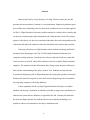
Most people learn by seeing, hearing, or feeling. Of these senses, the one that
generates the most productive learning is visual stimulation. Engineering students spend
most of their time calculating values for theoretical variables but never see them applied.
Cal Poly’s Flight Simulation Laboratory enables students to visualize these variables and
see them in action through cockpit instruments and 3-Dimensional visuals. The primary
purpose of this thesis is to develop a simulation laboratory that can be integrated into the
classrooms and enable the students to learn the simulation in the shortest time possible.
Not many schools have a flight simulator where students can design and build a
simulation from beginning to end. The Cal Poly Flight Simulation Laboratory has
computers, analog hardware, a simulator cab, software, and state-of-the art visuals that
create an entire set of tools, which allow students to become complete flight simulation
engineers. The students learn the information that is being sent to the pilot, which gives
them a better understanding of the pilot’s point of view. Students not only learn the
Aeronautical Engineering side of flight simulation (developing the equations of motion),
but they also learn the Computer Science and Electrical Engineering side of simulation
by integrating computers with analog hardware.
Future capabilities for the Cal Poly Flight Simulation Laboratory are endless.
Students can develop a simulation as detailed as possible as long as new simulations are
added to the system and new hardware is upgraded to the lab. Currently the laboratory
has only one flight simulator, but with the advent of new dynamic technology, it is
possible to add several simulators to develop a simulation arena.
iii
Acknowledgements
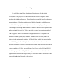
I would like to thank Doug Hiranaka and Fritz Anderson for their initial
development of this project. Fritz Anderson created the hardware integration of the
simulator cab with the software code. Doug Hiranaka developed the interface of the nonlinear, six-degree-of-freedom simulation using Matlab’s Simulink. I would like to also
thank the following people for their help on the simulator during the past few years.
Aaron Munger’s knowledge on the simulator’s hardware aided in the development of the
analog section of this thesis. Jon Tonkyro provided expertise in networking and helped
with the graphics. Edwin Casco and Paul Patangui assisted in the development of an
Instrument Landing System (ILS) Simulation. Members from the Spring AERO 320
helped with the engine model simulation. Jeff Nadel helped with the lab networking for
the ATL building. Dan Powell helped with moving the simulator and electrical
assistance. Dr. Daniel J. Biezad’s continued efforts to make flight simulation and controls
a strong emphasis at Cal Poly, San Luis Obispo. David Lowe and the F-18 and UH-1N
simulation groups at Manned Flight Simulator gave me experience and insight on how
flight simulators should be developed. Finally, I would like to thank Linda Jarrard for her
support during the time I invested on this project.
iv
Table of Contents
1. Introduction ................................................................................................................... 1
1.1 Computers and Hardware.................................................................................. 1
1.2 Software ............................................................................................................ 1
1.3 Pheagle Archive ................................................................................................ 2
1.4 Research Objectives .......................................................................................... 3
Figure 1: Advanced Technologies Laboratories (ATL) .............................. 3
1.5 Continuing Research ......................................................................................... 4
2. Simulation Flow............................................................................................................. 5
Figure 2: Simulation Flow Schematic..................................................................... 5
2.1 Analog Input...................................................................................................... 6
Figure 3: Analog Input Schematic .............................................................. 6
2.1.1 Stick.................................................................................................... 7
Figure 4: F-15 Stick ........................................................................ 7
Figure 5: Stick Torque Motor ......................................................... 8
2.1.2 Rudder ................................................................................................ 8
Figure 6: Rudder Torque Motor ..................................................... 8
2.1.3 Throttles ............................................................................................. 9
Figure 7: Throttles .......................................................................... 9
2.1.4 Consoles ............................................................................................. 9
Figure 8: Left Console Card ........................................................... 9
2.1.5 Stick Computer................................................................................. 10
v
Figure 9: Stick Computer.............................................................. 10
2.1.6 Siblinc .............................................................................................. 11
Figure 10: Siblinc.......................................................................... 11
2.1.7 Trace Card ........................................................................................ 11
Figure 11: Trace Card .................................................................. 11
2.2 Computer Hardware ........................................................................................ 13
Figure 12: Instructor Operating Station (IOS) ......................................... 13
2.3 Computer Software ......................................................................................... 14
2.3.1 Simulink and Real-Time Work shop................................................ 14
2.3.2 S-Functions....................................................................................... 15
2.3.3 C-Code ............................................................................................. 15
2.3.4 TCP-IP/UDP..................................................................................... 15
2.3.5 OpenGVS ......................................................................................... 16
2.3.6 D/A A/D Channel............................................................................. 17
2.4 Analog Output ................................................................................................. 19
Figure 13: Analog Output Schematic........................................................ 19
2.4.1 Stick and Rudder Signals ................................................................. 20
2.4.2 Instrument and Console Signals....................................................... 20
Figure 14: IJ1 & IJ2 ..................................................................... 20
Figure 15: Instrument Connections .............................................. 20
2.5 Visual Output .................................................................................................. 21
2.5.1 Front Cockpit Visuals....................................................................... 21
Figure 16: Front Cockpit Visuals ................................................. 21
vi
Figure 17: Front Cockpit IOS....................................................... 22
2.5.2 Rear Cockpit Visuals........................................................................ 22
Figure 18: Rear Cockpit Visuals................................................... 22
Figure 19: Rear Cockpit IOS ........................................................ 22
3. Simulation Operations Procedures............................................................................ 24
3.1 PhEagle Operations Manual............................................................................ 24
3.2 PhEagle Virtual Library .................................................................................. 24
3.2.1 Models.............................................................................................. 25
3.2.1.1 Stick Model ....................................................................... 25
Figure 20: Stick Model...................................................... 25
3.2.1.2 Engine Model .................................................................... 26
Figure 21: Engine Model .................................................. 26
3.2.1.3 Standard Atmosphere Model............................................. 27
Figure 22: Standard Atmosphere Model........................... 27
3.2.1.4 SixDOF Model .................................................................. 27
Figure 23: SixDOF............................................................ 27
3.2.1.5 Instrument Model .............................................................. 28
Figure 24: Instrument Model ............................................ 28
3.2.1.6 Graphics Model ................................................................. 28
Figure 25: Graphics Model............................................... 28
3.2.1.7 ILS Model ......................................................................... 29
Figure 26: ILS Model........................................................ 29
3.2.2 Tutorials ........................................................................................... 29
vii
3.2.2.1 Times Two Tutorial........................................................... 30
3.2.2.2 Speed of Sound Tutorial.................................................... 30
3.2.3 Documentation ................................................................................. 30
4. Simulation Development............................................................................................. 31
4.1 Graphics .......................................................................................................... 31
Figure 27: Pilot Verification..................................................................... 31
4.1.1 Terrain Database .............................................................................. 32
Figure 28: Korean Database ........................................................ 32
Figure 29: Monterey Database ..................................................... 32
4.1.2 Instrument Landing Simulation........................................................ 32
Figure 30: Takeoff / Landing Scenario ......................................... 33
Figure 31: CDI & ILS ................................................................... 34
4.2 Rear Cockpit.................................................................................................... 34
4.3 Heads-Up Display ........................................................................................... 35
4.4 Combat Simulator ........................................................................................... 35
4.5 Combat Simulation Arena............................................................................... 35
4.6 Projectors......................................................................................................... 36
Figure 32: Projector Setup ....................................................................... 36
Figure 33: Three-Projector Display ......................................................... 37
4.7 Calibration....................................................................................................... 37
4.7.1 Instrument Calibration...................................................................... 37
Table 1: Instrument Checklist ....................................................... 38
viii
4.7.2 Throttle Calibration .......................................................................... 38
Figure 34: Initial Throttle Readings ............................................. 39
Figure 35: Throttle Analog Output ............................................... 40
Figure 36: Corrected Throttle Output .......................................... 40
4.8 Graphical User Interface (GUI)....................................................................... 41
5. Simulator Implementation ......................................................................................... 42
5.1 Stability Derivatives........................................................................................ 42
5.2 Flight Control System Design ......................................................................... 43
Figure 37: Glide Slope Simulation............................................................ 43
5.3 VFR & IFR Landing Simulation..................................................................... 43
5.4 Guidance & Control ........................................................................................ 44
6. Conclusion.................................................................................................................... 45
ix
1. Introduction:
Flight simulations take years to develop. In industry, a team of 50 or more
engineers work on the simulation for a simulator, which allows it to become as real as
possible. Industry simulation labs contain several networked simulators to create a
simulation arena. The goal of Cal Poly’s Flight Simulation Laboratory is to develop a
multi-role simulator within a simulation arena. This will enable the simulator to model
any aircraft and will allow several aircraft to fly within the same three-dimensional
world. To accomplish this goal, years must be invested to develop the code to run the
simulation.
Simulations are quite complex. Flight simulation engineers must not only know
basic aircraft dynamics and controls, but they must also understand programming,
networking knowledge, hardware, standards, etc. This thesis develops a baseline for
achieving the simulation arena goal and sets a standard for training a flight simulation
engineer.
1.1 Computers and Hardware
The flight simulator consists of the Pheagle cab and two analog computers, which
complete the link between the digital computers. The simulation is affordable because it
uses four Pentium 166 computers and common software. This also allows the
communication from the analog realm to be accessed from the digital realm with the use
of A/D and D/A cards. Since the digital realm is split into multiple computers, the
computing power is endless. As processors and graphic cards become faster and better,
1
the simulation is transportable to any platform. More digital and analog hardware can be
implemented in the simulation allowing further research into futuristic cockpit displays or
imbedded avionics. Due to the networking capability of the simulation, simulators can be
added as long as there is enough bandwidth. Desktop simulators or other analog
simulators can be added to the simulation to develop a simulation arena.
1.2 Software
The simulation integrates C-code with Matlab’s Simulink S-Function Applied
Programmer’s Interface (API). Simulink’s Graphical User Interface (GUI) allows the
user to see the variables flow through the simulation. At any time, the user can monitor or
graphically display one of the variables and plot it as a function of time. This is far better
than debugging in most common compilers since Simulink allows the programmer to see
the variables in real-time. Simulink also allows the simulation to be broken down into
subsystems and individual simulation models. These models can be individually tested or
added to a completely different simulation.
Simulink’s S-Function API allows any C-Code to be integrated into the
simulation. This allows the implementation of other API’s into the simulation. OpenGVS
is another API that uses OpenGL code to generate a Realtime Scene Management for
Three-Dimensional Visuals. OpenGVS has specific functions that enable the threedimensional environment to be changed such as camera position, lighting, and visibility.
1.3 PhEagle Archive
2
The simulation laboratory needs to continue its ongoing development. This means
that running and developing the simulator needs to become easy to learn in the shortest
time possible. The development of the PhEagle Virtual Library enables senior projects,
thesis work, research, and simulation models to be well documented, stored, and easily
accessible, so students can begin where the last student finished. This will allow the
simulator’s development to be ongoing and keep up with industry. Included are tutorials
and demos, which teach the students how to create a simulation and learn different
aspects of the simulator. The Pheagle Operations Manual thoroughly describes how to
run the simulator and how to test and calibrate any of the hardware, instruments, or
simulations.
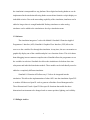
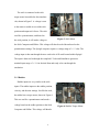
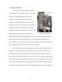
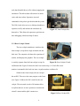
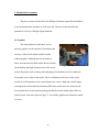
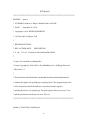
1.4 Research Objectives
The initial goal was to develop a visual system
for the simulator that led to the development of an
Instrument Landing System (ILS) Simulation. Before
this could happen, the simulator had to be moved into
the new Northrop Grumman Aerospace System
Laboratory in the Advanced Technology Laboratories
(ATL) building at Cal Poly, San Luis Obispo, shown
in Figure 1. This led to the development of the new
Figure 1:
Advanced Technologies Laboratories
(ATL)
simulation laboratory.
In order for the ILS simulation to work, an adequate engine model had to be
developed. Also the ILS and CDI instruments were not working at the time of
3
development. These models had to be generated, calibrated, and tested. Once these were
completed, the graphics had to be implemented into the simulation complete with an
airport and terrain database. Once completed, the simulation starts the aircraft at a
distance from the airport where the pilot uses the instruments along with the visuals to
land the aircraft at the airport.
1.5 Continuing Research
The next step is to integrate multiple aircraft into the simulation arena. The
simulator cab is a two-seater, which allows the addition of another cockpit. The rear
cockpit is entirely digital complete with a flat screen display, a gaming joystick, throttle,
and rudder pedals. This will enable the simulator to have “dog fighting” capability. Since
the rear cockpit is entirely digital, it can be copied to create another desktop simulator,
which can be added to the simulation to create a flight simulation arena.
4
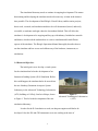
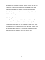
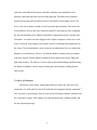
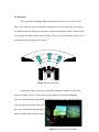
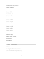
2 Simulation Flow:
The PhEagle Flight Simulator is quite complex due to the interaction between the
digital and analog signals; therefore, it is important to understand the signal flow of the
simulation. This enables the operator to be able to trace a signal to see if it is getting to
and from the simulator cab. Figure 2 gives a simplified description of the input and
output signals to and from the cab, the analog computers, and the digital computers. The
yellow arrows represent inputs to the I/O computer, Spiegel, and the green arrows
represent the outputs. In general the cab sends stick and rudder inputs to the stick
computer, and throttle inputs are sent to Siblinc. The signal then gets mapped to A/D
cards located in Spiegel through the trace card. Spiegel then computes the equations of
motion to generate the states of the aircraft. The position and orientation is sent to each of
the three visual computers, Eagle, Phantom, and Pheagle, which display the center, left,
Instruments & Lights
Phantom
(Left View)
Throttle Inputs
Spiegel
Siblinc
Trace
Card
PhEagle CAB
(EOM)
Stick & Rudder
Inputs
E
T
H
E
R
N
E
T
Eagle
(Center View)
Pheagle
(Right View)
Stick
Computer
Stick & Rudder Forces
Figure 2: Simulation Flow Schematic
5
and right views respectively.
Spiegel also sends out analog signals to the cab. Instrument settings and lights are
sent through Spiegel to Siblinc then to the cockpit. Stick and Rudder forces are sent to the
stick computer and then to the stick and rudder to generate force-feed back. Each of these
sections will be broken down to give a more detailed description of the signal flow.
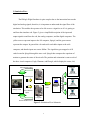
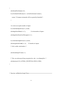
2.1 Analog Input
The incoming analog signal to Spiegel reads the signals from the stick, rudder,
and throttle and the left and right console panels. Figure 3 shows a schematic of the
analog input from the stick, rudder, throttle, and consoles to the I/O computer, Spiegel.
Trace
Card
Stick & Rudder
Motors
Stick
Stick Computer
Bottom Torque
Motor Assembly
Cockpit Junction
Box (CJB)
Spiegel
Rudder
Throttle Card
Trace
Card
Throttles
and
J – Connectors
Left Console
Card
Left Console
Siblinc
Right Console
Card
Right Console
Figure 3: Analog Input Schematic
6
The analog inputs are broken down into control inputs or switches. Control inputs
include the stick, rudder, and throttle inputs. Switches include any of the switches
located on the consoles, the stick, or the throttle. The stick and rudder inputs send signals
to both the Siblinc and the Stick Computer. The throttle is located on the left console and
is connected to the left console card. Both console cards connect to the Cockpit Junction
Box (CJB) located beneath the simulator. Any signals connected to the CJB get sent to
Siblinc.
Control inputs send voltage signals to Siblinc and/or the Stick Computer based on
the control device. These inputs then get scaled to a range of +/- 5 volts. This voltage is
then sent to the trace card where the signals are broken down to the desired pin
arrangement for the corresponding A/D card, located within Spiegel.
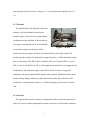
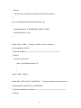
2.1.1 Stick
Stick inputs can be the stick position,
velocity, and stick trim settings as well as the
buttons located on the stick such as the trigger
and the hat switch. Originally the simulator cab
was an F-4 Phantom simulator. The stick is an
F-15 Eagle stick, shown in Figure 4, which was
added to the simulator for handling qualities
research at NASA Dryden. Hence, with the
Figure 4: F-15 Stick
combination of the two, the simulator received
its name PhEagle.
7
The stick is connected to the stick
torque motor located below the simulator
cab, shown in Figure 5. A voltage is sent
to the motor to enable it to read the stick
position and output stick forces. The stick
acts like a potentiometer, and based on
Figure 5: Stick Motor
the stick position, it will send a voltage to
the Stick Computer and Siblinc. This voltage will then be scaled down based on the
potentiometer settings. The Spiegel computer requires a voltage range of +/- 5 volts. The
voltage input is then ran through the trace card to the A/D cards located within Spiegel.
The input is then read in through the compiled C-Code and Simulink to generate a
nominal input range of +/- 1.0 in decimal form and ready to be run through the
simulation.
2.1.2 Rudder
Rudder inputs are very similar to the stick
inputs. The rudder inputs are the rudder position,
velocity, and the trim settings. Just like the stick,
the rudder has a torque motor, shown in Figure 6.
This too acts like a potentiometer and sends a
voltage based on the rudder position to the Stick
Figure 6: Rudder Torque Motor
Computer and Siblinc. This voltage will then be
8
scaled down just like the stick to a range of +/- 5 volts and generate a digital value of +/1.0.
2.1.3 Throttles
The throttle input is the right and left throttle
setting as well as the buttons located on the
throttles. Figure 7 shows the two-engine throttle
configuration in the simulator. If the aircraft has
two engines, each throttle can be set individually
Figure 7: Throttles
to control the output of each engine. If the
aircraft has only one engine, the thrust is divided in half by each engine setting. The
throttle generates an input of a nominal percentage from 0 to 1. Within the throttle region
there are four stops: OFF, IDLE, MIL, and MAX. OFF is at 0% thrust, IDLE is at 10 %,
MIL is at 62 %, and MAX is at 100 %. If the engine being modeled is a jet equipped with
an afterburner, the afterburner range is from MIL to MAX. In order to engage the
afterburners, the grasps underneath the throttle must be pulled. Additional buttons on the
throttle are flap settings, rudder trim, and buttons and switches that could be used for
speed brakes, communication buttons, etc. All throttle inputs get fed to the left console
card.
2.1.4 Consoles
The right and left console each have an independent card to read in the input such as
pitch, roll, and yaw control augmentation switches, stick force on/off switches, and more.
9
Currently, the only console card integrated
into the simulation is the left console card,
shown in Figure 8. There are additional
cards for both the left and right console. To
receive inputs from the right console, the
right console card would have to be
Figure 8: Left Console Card
mounted and connected into the simulator.
2.1.5 Stick Computer
The stick computer controls the inputs and
outputs to and from the stick and rudder
motors. The most important feature of the
stick computer is that it can generate excellent
stick and rudder feel since its main purpose
was for handling qualities research. The stick
computer is broken into three sections: pitch,
roll, and yaw. The three axial forces can be
modified for force gradients, damping,
breakout, and stop locations. Figure 9 shows
Figure 9: Stick Computer
the stick computer with the different potentiometers located on the front panels. Other
important features on the analog computer are trim settings, surface position, and amount
of force generated by the motors. Each motor has the capability of generating 50 pounds
of force.
10
2.1.6 Siblinc
Siblinc is the other analog computer that
controls the channels being sent to and from the
cab. 1 Figure 10 shows Siblinc with its many
channels located on the front panel. Each channel
has three potentiometers. These set the NULL,
BIAS, and SCALE for each channel. The middle
section of Siblinc contains a patch voltmeter that
allows each signal to be monitor coming into
Siblinc and going out of Siblinc. The bottom
Figure 10: Siblinc
section contains additional channels for switches and lights. The main purpose of Siblinc
is to modify the signal going to and from the cab so that the output or input voltage of the
cab is scaled to +/- 5 volts for the I/O computer, Spiegel.
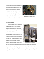
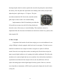
2.1.7 Trace Card
The trace card is the key to break the gap from
the analog realm to the digital realm. 2 Figure 11
shows the green trace card located on the back of
cabinet of the instructor operating station. This card
allows each channel to be split up into either an
input or and output. If the signal is an input signal, it
goes to one of the A/D PC lab cards. If the signal is
Figure 11: Trace Card
11
an output, it is sent from either the 16 bit D/A card, or the 12 bit D/A card. The trace
card receives three connectors from Siblinc. An additional connector is also sent from
Siblinc, however, the channels within this connector are not known. To add these
channels to the simulation another trace card would need to be added as well as some
additional A/D and D/A cards. Luckily, additional cards are located within the hardware
cabinet.
12
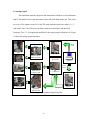
2.2 Computer Hardware
The computers integrated into the simulation
are four Pentium 166 computers. Figure 12 shows the
Instructor Operating Station (IOS) where each
computer is mounted within the cabinet. Each
computer serves a distinct purpose. This allows the
simulation to be run in real-time since each computer
is designated for a specific task. The I/O Computer
contains four data acquisition cards: a 16 and a 12 bit
Digital-to-Analog (D/A) card, a 12 bit Analog-to-
Figure 12: Instructor
Operating Station (IOS)
Digital (A/D) card, and a 48 bit digital input/output card. The I/O computer handles the
analog inputs and outputs to the simulation as well as computing the Equations Of
Motion (EOM) to solve for the aircraft’s position, orientation, and state, which are sent to
the two analog computers as well as the three visual computers.
Each of the four digital computers contains a network card and can communicate
through a network hub, which creates a Local Area Network (LAN), or Intranet. The
I/O computer acts as a server and sends the aircraft’s position, orientation, and state, to
each of the visual computers, which act as clients. Each visual computer is equipped with
an Obsidian 2 Quantum 3D graphics card, which is basically a modified 3Dfx Voodoo 2
card. Each of these cards is set to run the glide hardware. Additional hardware is sound
cards located within Eagle and Pheagle, and additional data acquisition cards in Phantom.
13
2.3 Computer Software
The four computers each run Windows 95 as their operating system. This allows
any windows applications to be implemented in the simulation. Older simulation
laboratories use VAX or VMS machines to run the simulation. With the advent of faster,
low cost PC’s, the Windows platform allows students to work in a familiar environment.
This also allows the portability of adding new software to the simulation.
Currently, the computers are equipped with MATLAB, Simulink, and the Real
Time Workshop to run the simulation. 3 These computers use Visual C++ 6.0 to compile
the simulation code, and the visual software is generated using OpenGVS.
2.3.1 Simulink and the Real-Time Workshop
The PhEagle simulation runs in Simulink by MATLAB. If the simulation was left
entirely as code, the programmer would be lost not knowing which variables were being
sent, which variable names are being used, and the file order. Simulink allows this
process to become simple. Simulink allows the students to visually map the variables as
the simulation computes them. Simulink also allows the users to easily grab a variable
and monitor it or link it to a subsystem within the simulation. Variable names don’t have
to match for the code to run. The file order is easy to see as the programmer can follow
the flow of the simulation and visually see the order that files get called within the
simulation.
The Real-Time Workshop allows the simulation time-differential to be changed. 4
This allows a more accurate integration to keep the simulation running in real time. This
14
also allows the entire simulation to be compiled into one executable. Programs can be
generated, distributed, then tested in the classrooms, or students can use them at home.
2.3.2 S-Functions
The Real-Time Workshop in conjunction with Simulink requires the code to be
written in a special S-Function format. 5 This allows different sections of the code to be
run at different times during the simulation.6 For instance, the S-Function requires the
code to have a start, initialize, sample time, output, and termination sections. The start
section is only called the first time the simulation runs. The initialize section initializes
the size of the input and output arrays. The sample time section determines the time
differential for the simulation. The output section computes the output variables. The
termination section allows conditions to be set to terminate the simulation. Various other
sections can be added to make the code behave how and when the programmer wants it
to.
2.3.3 C-Code
The C-Code for the simulation is written in the S-Function format.7 If the code is
in the correct format, the compiler will generate a dynamic linked library (dll). This is
compiled C-Code much like an executable. Simulink searches for this dll based on the SFunction name that was assigned to it. To generate the dll, the compiler must be set up
correctly so Matlab knows where to find it. The code cannot be written in C++, it must
only be written in C. The entire code for the simulation was written by students.
15
2.3.4 TCP-IP/UDP
Since the computers are networked together, code had to be written to
communicate between the two. The goal was to have the I/O computer, Spiegel, compute
the aircraft’s position and orientation and send that information to the other three visual
computers to generate the graphics. A sample program was written in C++ for a UNIX
platform to test the functionality of sending information across the Internet. 8 One side of
the program acted as the server and the other program played the client. This program
then had to be modified to work under Windows using winsockets. Once the program
proved to work, it had to be modified again to work using UDP. UDP is similar to TCP
except that it allows the communication to be connectionless. Once the program was
working, the code had to be converted to C then added to a test bed simulation within
Simulink. The program was tested, and it worked perfectly with little lag in the frame
rate. The final step was to have the test bed simulation work with the graphics since the
communication barrier had been breached; the next step was to have the model work with
the graphics.
2.3.5 OpenGVS
OpenGVS offers excellent 3-D rendering scene software that is already set up for
flight simulation.9 OpenGVS already has imbedded functions that allow terrain databases,
camera views, vehicles, lighting, etc. to be simply added to the simulation. Included
within OpenGVS are demo programs that give a programmer an idea of how to create
visuals. The demos include a Heads-Up-Display (HUD) demo that has an aircraft fly
through a database of Korea in a Mig-29 armed with missiles. Other demos include a
16
tank demo with different helicopters and tanks within the same battlefield, and a
Monterey demo that starts the aircraft in final approach. The demos also included a
master/slave program that would be perfect as a baseline for networking visuals. The
server code was created to send the aircraft’s position and orientation. The client code
was modified to work as the slave within the OpenGVS environment. Once completed,
the aircraft simulation ran in Matlab’s Simulink to compute the aircraft’s position and
orientation. It was then sent from Spiegel to the Graphic computers via the server code,
where a client on each computer received the aircraft’s information and displayed it on
the screen. The terrain database can be chosen by an initialization file as to whether the
database is to be Monterey or Korea. The Korean database contains snowy mountains
with deep canyons, and the Monterey database has an airport with runway lights and
glide slope markers. The objective is to develop an instrument landing simulation using
the Monterey database with the airport and integrate an Instrument Landing System
(ILS) model.
2.3.6 D/A A/D Channel
Besides the visual output, analog output had to be sent to the cab to drive the
instruments. To do this the D/A and A/D cards had to be integrated into the simulation 10.
This was done by developing a class for each card and creating a channel within the class
for each input or output. Each channel is set and initialized with a channel number and
the max input/output range.
17
2.4 Analog Output
The simulation sends the outputs to the instruments with the use of an instrument
model. This model receives the instrument values and sends them to the cab. The values
are set to a D/A channel on the D/A card. The card sends the signal on a range of +/- 5
volts to the Trace Card. The trace card then connects to the Siblinc and the Stick
Computer. The +/-5 volt signal gets modified for the analog target within the cab. Figure
13 shows the analog output schematic.
Trace
Card
Stick & Rudder
Motors
Stick
Stick Computer
Bottom Torque
Motor Assembly
Cockpit Junction
Box (CJB)
Spiegel
Rudder
Trace
Card
L & R Console
and
J – Connectors
Right & Left
Console Cards
Instruments
Siblinc
Instrument
Motherboard
Figure 13: Analog Output Schematic
18
2.4.1 Stick and Rudder Signals
The stick and rudder can receive stick force commands from the simulation based
on the amount of g’s being generated by the aircraft maneuvers. This force is sent to the
stick computer, which sends the signal to the stick and rudder torque motors to generate
the force. These forces can generate up to 50 pounds of force.
2.4.2 Instrument and Console Signals
From Siblinc, several connectors split the signal
from Siblinc to the instruments and consoles. Initially, the
signal gets sent to the cockpit junction box (CJB) where it
then gets sent to the instrument panel motherboard
assembly. Two connectors attach the signals to the
motherboard, these are known as IJ1 & IJ2. Figure14
shows these connectors mounted to the motherboard. The
signal finally reaches its destination target by a connection
Figure 14: IJ1 &IJ2
to one of the instruments from the motherboard.
Figure 15 shows the back of the
instruments with their connections linking them to
the motherboard assembly. A tag on each
instrument describes the channel number of the
instrument. This is the same channel as on Siblinc.
19
Figure 15: Instrument Connections
This channel also is etched into the motherboard. The Model II Cockpit, Book IV 11
describes the electrical connections in detail with schematics and tables for each wiring
connection.
2.5 Visual Output
The visual output is split up into two sections, the front cockpit visuals and the
rear cockpit visuals. Each displays the pilot’s visuals and the Instructor Operating Station
(IOS) visuals.
2.5.1 Front Cockpit Visuals
The Spiegel computer also sends information about the aircraft to the visual
computers. Figure 16 shows the front cockpit
visuals. The visuals are setup to generate three
views. Eagle is designated as the center visual
computer. Eagle will display the center view as
well as the HUD. Phantom and Pheagle will
display the left and right views respectively.
Figure 16: Front Cockpit Visuals
The visuals can be either a Monterey database with an airport, or a Korean database with
mountains.
The pilot and the IOS have a set of visuals. Figure 17 shows the IOS visuals. The
IOS visuals are the same as the pilot’s visuals. This allows the operator to see where the
aircraft is flying and still be able to monitor the state of the aircraft within the Simulink
simulation window. Also the operator can generate charts in real time or use any other
20
tools that Simulink has to offer without stopping the
simulation. This allows data collection to be much
easier and more robust. Operators can send
commands to the pilot to get the data that they want.
The IOS visuals also serve as a desktop simulator so
operators can fly and monitor the simulation by
Figure 17: Front Cockpit IOS
themselves. This allows the operator to perform run
time debugging without the help of others.
2.5.1 Rear Cockpit Visuals
The rear cockpit simulation is similar to the
front cockpit, except that a single machine runs the
back seat. The computer calculates the equations of
motion, and displays the graphics. The rear cockpit
is entirely separate from the front cockpit except for
Figure 18: Rear Cockpit Visuals
an Ethernet link. Figure 18 shows the back seat visual setup. A 15-inch flat screen
monitor is mounted in the back seat since a regular monitor would not fit.
Similar to the front cockpit, the rear cockpit
has an IOS. This serves the same purpose as the front
seat. Figure 19 Shows the IOS visuals for the rear
cockpit. The increased visuals of all stations allow
two pilots and two or more operators to monitor the
aircraft’s states and the pilot’s maneuvers.
Figure 19: Rear Cockpit IOS
21
3. Simulation Operations Procedures:
The hardest task for students working on this simulator is trying to understand
how it works. Due to its initial development there are little resources that explain how the
simulator works. In order for the learning curve to decrease, adequate documentation and
resources need to be made available for the next student working on this project. The
PhEagle Operations Manual, and the PhEagle Virtual Library contain descriptions and
procedures of how to run the simulator, where to store back-up files, model descriptions,
tutorials, and documentation. Each student working on the simulator will update the
PhEagle Operations Manual, and the PhEagle Virtual Library.
3.1 PhEagle Operations Manual
The PhEagle Operations Manual contains operations and procedures of how to
run the simulator.12 Also included are references of student work such as previous
operation manuals, student senior projects, and theses. Software, hardware, and API
implementation are included such as Matlab GUI documentation, TCP/IP and UDP
documentation, A/D and D/A card information. Most importantly, the source code is
printed out and located in its appropriate section describing the model.
3.2 PhEagle Virtual Library
The PhEagle Virtual Library is much like the PhEagle Operations Manual except
that it is Web based. This allows a tree structure library to store documentation, code, and
any other pertinent information into subsequent directories. Within the library is a
22
description of each model, the corresponding code, model file, executable, and
documentation. Also included are tutorials in HTML format. This describes a step by step
format on how to compile code, generate models, and repeat any process that has been
done before. The last aspect of the PhEagle Virtual Library is its documentation database.
This will include any thesis work, senior projects, student work, or pertinent information.
3.2.1 Models
Within the PhEagle Virtual Library are model sections describing each model in
detail. Included in each section are the Simulink model, source code, executable (dll) and
any documentation. Any updates to the source code or models is to be updated to the
directory for that model so that all models and code is current. The following are the
models entered so far in the simulation.
3.2.1.1 Stick Model
The stick model in Figure 20 reads the inputs
from the stick, rudder, and throttles. The input is on
a range of +/-5 volts and outputs +/- 1.0 in digital
form to be run in Simulink for the stick and rudder
pedals. For the throttle inputs the output is in
percent of maximum thrust. This will base the
Figure 20: Stick Model
throttle setting from 0 to 1.
23
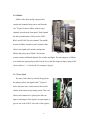
3.2.1.2 Engine Model
The engine model in Figure 21 computes the thrust generated by the aircraft’s
engine(s) based on the throttle setting, altitude, and static seal level thrust.13 The engine
can either be a propeller, turboprop, high by-pass ratio engine, or jet engine with
afterburner or without.14 Other necessary inputs are left and right engine fuel capacity,
propeller efficiency (if a propeller driven engine), TSFC, and afterburner TSFC. It then
computes the thrust generated based on these inputs and calculates the engine RPM,
temperature, fuel flow, and nozzle position.
Figure 21: Engine Model
24
3.2.1.3 Standard Atmosphere Model
The Standard Atmosphere Model
is shown in Figure 22. This model
computes the speed of sound, density,
pressure, and temperature, based on
altitude. This model also takes into
account the different altitude regimes that
Figure 22: Standard Atmosphere Model
the aircraft is flying in and applies the
appropriate equations.
3.2.1.4 SixDOF Model
This model computes the
aircraft’s position and orientation
along with velocity, angular rates,
angle of attack, sideslip, and
translational accelerations. The
SixDOF model in Figure 23 treats
the aircraft like a point mass. It
Figure 23: SixDOF Model
converts the forces, moments,
and control inputs generated by the aircraft to compute the above states. The term six
degrees of freedom refers to the translational and rotational positions: X, Y, Z, and Psi,
Theta, Phi. The model also reads in a Standard Aircraft Data (SAD) file, which contains
the aircraft’s stability derivatives and initial conditions.
25
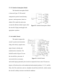
3.2.1.5 Instrument Model
The instrument model in Figure 24
receives the inputs from the SixDOF model. This
model initializes the instruments and sets the
range of the instruments. The model then sends
the values to the D/A cards, which convert it to a
range of +/- 5 volts. This communication is done
through the use of the DA Channel class. This is
an excellent model for testing and calibrating the
Figure 24: Instrument Model
instruments and channels.
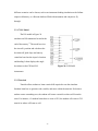
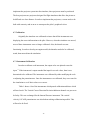
3.2.1.6 Graphics Model
The graphics model receives the position and
rotation from the SixDOF model as well. It sends the
information over the Ethernet to the three graphics
computers using UDP. The model waits for the graphics
to initialize before it starts the simulation. It also does a
conversion from aircraft axis to world axis. Figure 25
shows the graphics model with the three outgoing
Figure 25: Graphics Model
signals to each computer that send the aircraft’s position
and orientation as well as whether to keep the graphics running. On the client side,
26
different scenarios can be chosen, such as an instrument landing simulation to the Salinas
airport in Monterey, or a Korean database filled with mountains and canyons to fly
through.
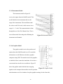
3.2.1.7 ILS Model
The ILS model in Figure 26
simulates an ILS transmitter located at the
end of the runway.15 The model receives
the aircraft’s position and calculates the
deviation off glide-slope and runway
centerline based on the airport’s location
and heading. It then displays the angle
Figure 26: ILS Model
deviations on the CDI and ILS
instruments.
3.2.2 Tutorials
Tutorials allow students to learn certain skills required to run the simulator.
Students learn how to generate code, models, and more within the tutorials. Each time a
student creates something new, the student will create a tutorial so others will learn the
same. For instance, if a student learns how to create a GUI, the student will create a GUI
tutorial so others will learn as well.
27
3.2.2.1 Times Two Tutorial
This is a simple tutorial that teaches the students how to compile code in Matlab.
Although this is a simple model, since it computes the input by two, the code is quite
complex. To do this simple model will require two pages of code.
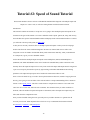
3.2.2.2 Speed of Sound Tutorial
This is a more complex tutorial where the student has to create the code and
model from scratch. Students here learn the basic S-Function format. The model receives
the gamma, gas constant, temperature, and velocity, and computes the speed of sound and
Mach number.
3.2.3 Documentation
Any documentation written for the simulator or that pertains to the simulator is to
be stored in the documentation directory. This primarily includes student work such as
theses, senior projects, class or project work, etc. Additional documentation are helpful
references that pertain to the simulator development such as military standards, FAA
guidelines, software documentation that pertains to Matlab, Simulink, OpenGVS,
TCP/IP, UDP, etc.
28
4. Simulation Development:
The prior sections described how the PhEagle Simulator signals flowed and how
to run and maintain the simulator as well as the lab. The next section describes the
potential of Cal Poly’s PhEagle Flight Simulator.
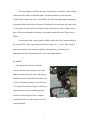
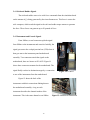
4.1 Graphics
The main emphasis of this thesis was to
generate graphics for the simulator. Determining the
accuracy of the aircraft model would be harder
without graphics. Although the aircraft model is
linear, the non-linear SixDOF model did an excellent
Figure 27: Pilot Verification
job mimicking the flight characteristics of the actual
aircraft. Responses such as short period and phugoid oscillations as well as dutch roll
movements were evident in the model. These oscillations would occur in the actual
aircraft as well. Responses to the control inputs were correct. High gain control inputs
would generate a Pilot Induced Oscillation (PIO) that would cause loss of the aircraft.
Several pilots flew in the simulator and agreed that the aircraft model behaved like an
actual aircraft, such as the pilot in Figure 27. Overall the graphics proved that the model
is correct.
29
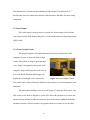
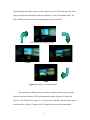
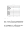
4.1.1 Terrain Database
Further development of the graphics lead to the ease of the capability of
OpenGVS. Different terrain models could be chosen to allow the pilot to fly in a Korean
database, shown in Figure 28, filled with mountains, or a Monterey Database equipped
with an airport, shown in Figure 29. Additional terrain databases can be added to the
simulation as long as they are in the correct format.
Figure 28: Korean Database
Figure 29: Monterey Database
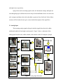
4.1.2. Instrument Landing Simulation
The objective of this thesis was to develop an Instrument Landing Simulation
complete with an airport and an ILS simulation. To make the OpenGVS database
compatible with our simulation, a coordinate transformation had to be performed. The
OpenGVS world axis were –Z, Y, X in relation to the aircraft axis X, Y, Z. A simple
modification generated the correct output to make the two worlds compatible. Finally, the
bridge between OpenGVS and Simulink had been crossed.
The Instrument Landing Simulation forces the student pilot to become familiar
with the ILS. Figure 30 shows a typical takeoff / landing scenario for a student pilot’s
training mission. The aircraft can either start two miles away from the airport on the
30
downward approach of the runway or on the airport’s taxiway. If the aircraft starts at the
airport, the pilot will takeoff and climb to an altitude of 1,000 feet heading North. The
pilot will then proceed to enter the landing pattern as they turn South.
Turn to Intercept Landing Pattern
Runway Approach
Takeoff
Land
Figure 30: Takeoff / Landing Scenario
The pilot needs to align the aircraft with the centerline of the runway using the
Course Directional Indicator (CDI) and Instrument Landing System (ILS) shown in
Figure 31. The CDI shows a range of +/- 10 degrees off centerline. Once the pilot centers
in on the runway within 2.5 degrees, the ILS begins to move across the instrument
31
showing the pilot where he needs to position the aircraft to keep the plane centered down
the runway. Once the plane has acquired the same heading as the runway, the pilot must
adjust the plane’s glide-slope to –2.5 degrees. The pilot
must then maintain the ILS fixed on the centerline and the
glide-slope in order to make a nice smooth landing.
Implementation of the ILS simulation proved that the
ILS model was accurate since the ILS led the pilot directly
Figure 31: CDI & ILS
down the center of the runway to a smooth landing. This simulation can now be
implemented into the classrooms and students can learn how to takeoff, fly a pattern, then
land using the ILS.
4.2 Rear Cockpit
Completion of the baseline for the front cockpit gives rise to the addition of a rear
cockpit. PhEagle is already equipped with a back seat for a navigator. The back seat was
modified to enable the rear cockpit to be either a navigator or a pilot of a different
aircraft. Since the rear cockpit does not have an analog stick, like the front cockpit, the
input is purely digital with the use of a gaming stick, rudder, and throttle. This allows the
simulation to be entirely digital and run on one machine. Once the baseline simulation is
copied and created from the front cockpit to the rear, the only difference will be to
replace the analog input with the digital inputs from the joysticks. However, since the
rear cockpit has no instruments, a HUD must be generated to display the aircraft’s states
to the pilot.
32
4.3 Heads-Up Display
OpenGVS already has a demo model that creates a Heads-Up Display (HUD).
Implementing this demo into the simulation will allow the aircraft’s states to be displayed
on the center view for both the front and rear cockpits. The model already computes the
states needed, so all that needs to be done is to integrate the HUD into the simulation.
This can be done by sending a struct containing the aircraft states across the Ethernet to
the center computer.
4.4 Combat Simulator
Combat simulators require at least two or more vehicles. With the completion of
the rear cockpit baseline with a HUD, both simulations are ready for “dog fighting”.
Another model within OpenGVS uses a generic missile simulation that allows a missile
to be fired when a key is pressed. Implementing this model into the simulation will allow
the simulation to be “dog fight” capable. OpenGVS already has the demos set up to allow
the number of vehicles to change. Changing this variable to two allows the aircraft to fly
within the same three-dimensional world and see each other.
4.5 Combat Simulation Arena
A combat simulation arena is when more than two aircraft are fighting against
each other in the same world. Since the rear cockpit is entirely digital, adding another
desktop simulator to the simulation can be accomplished by repeating what was done for
the rear cockpit. This allows not only combat scenarios but also formation flying.
As many simulators can be added to the system as long as there is adequate bandwidth.
33
4.6 Projectors
The Visuals for the PhEagle flight simulator have been proven to work for all
three views. The next step is to determine what type of visual system to use. The choices
are either monitors or projectors. Projector screens can be aligned to offer a wider field of
view and give the pilot a better sense of flying. Figure 32 gives an example of how to set
up the projectors with the use of a screen.16
Figure 32: Projector Setup
A projector setup was tested to see how the simulator would look with a threeprojector system. Figure 33 shows the projector displays of the Korean database.
This was far better than having the three monitors display the views. The 120O field of
view gave the pilot a better sense of flying. The projectors were situated so that each of
the views would blend into the other. When the monitors were used, the pilot’s visual
display would consist of breaks causing discontinuity in the graphics. In order to
34
Figure 33: Three-Projector Display
implement the projector system into the simulator, three projectors must be purchased.
The best projectors are projectors designed for flight simulators that allow the picture to
be diffused at a close distance. In order to implement the projectors, a screen needs to be
built with concavity and at an arc to encompass the pilot’s peripheral vision.
4.7 Calibration
Originally the simulator was calibrated to insure that all the instruments were
displaying the correct information to the pilot. However, when the simulator was moved,
most of these instruments were no longer calibrated. Also, the throttle was not
functioning. In order to develop an engine model, the throttles needed to be calibrated,
tested, then entered into the simulation.
4.7.1 Instrument Calibration
In order to calibrate each instrument, the output value was plotted versus the
input. 17 If the instrument’s output matched the input for several values, then it was
determined to be calibrated. The instrument was calibrated by either modifying the code
or adjusting the potentiometers. Once the instruments were calibrated, they were tested in
the simulation to see if their values were correct.
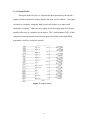
Table 1 shows a list of the instruments which passed calibration and those which
still need work. The Vertical Course Direction Deviation Indicator channel was proven to
be faulty. This was exchanged for the Internal Pressure instrument. The vertical
velocity’s SCALE potentiometer was also broken making calibration impossible. This
will need to be fixed.
35
Table 1: Instrument Calibration Checklist
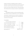
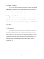
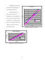
4.7.2 Throttle Calibration
In order to develop an engine model simulation the throttles needed to be
calibrated. This required the code to be modified as well as adjusting the potentiometers
on Siblinc. The goal was to have the throttles read the same output at the same location.
This is crucial since any error results in the loss or gain of thrust. Since the throttles are
based on a percentage, an error of 2% on a 10,000-pound engine results in a thrust error
of 200 pounds. This is sufficient and can cause the model to be inaccurate.
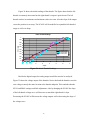
36
Figure 34 shows the initial readings of the throttle. The figure shows that the left
throttle is extremely inaccurate but the right throttle’s output is quite decent. The left
throttle reaches its maximums and minimum values too soon. Also the slope of the output
versus the position is too steep. The SCALE will be modified to expand the left throttle’s
range as well as its slope.
Initial Throttle Settings
1
0.9
0.8
% Throttle
0.7
0.6
0.5
R-Throttle (Fwd)
L-Throttle (Fwd)
R-Throttle (Rev)
L-Throttle (Rev)
0.4
0.3
0.2
0.1
0
0
1
2
3
4
5
6
7
X pos
Figure 34: Initial Throttle Readings
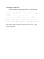
Besides the digital output, the analog output would also need to be analyzed.
Figure 35 shows the voltage output of the throttles. Notice that both the throttles cross the
zero voltage at nearly the same location at the throttle midpoint. This concludes that the
NULL and BIAS settings need little adjustment. Also by changing the SCALE the slope
of the left throttle voltage curve will decrease to match the right throttle’s slope.
Decreasing the SCALE will decrease the voltage outputs well as decreasing the slope of
the voltage curve.
37
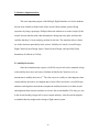
By adjusting the potentiometer
Analog Signals
settings, the final graph displays the
8
corrected output in Figure 36.
6
Both throttles follow each
4
other’s output with little error.
Voltage (V)
2
Originally the error in the throttle was
up to 16%. After calibration, this error
0
0
2
4
6
-2
R-Throttle TNK
was reduced 1-2%. A slight amount of
-4
backlash was found in the throttle due
-6
to hysteresis. This will need to be
-8
L-Throttle TNK
X-pos
assessed in the future.
Figure 35: Throttle Analog Output
Throttle Calibration
1
Output
0.8
0.6
0.4
R-Throttle
L-Throttle
0.2
0
0
2
4
Position
6
8
Figure 36: Corrected Throttle Output
38
8
4.8 Graphical User Interface (GUI)
A graphical user interface will allow different options to be changed easily within
the simulation. Matlab already has a Graphical User Interface Design Environment
(GUIDE) that would allow GUI implementation to be easy to add into the simulation. 18
This GUI will allow the user to input different initial conditions such as airport or
database location, wind and atmospheric conditions, aircraft, time of day, visibility, etc.
Modification of the GUI could incorporate graphics such as graphs, a display of the
ownship’s attitude with a 3-D model, stick position, etc. 19 Additional GUIs can be added
to the simulation with the use of Microsoft Foundation Classes (MFC), which are useful
in Windows applications. 20
39
5. Simulator Implementation:
The most important purpose of the PhEagle Flight Simulator is to let the students
become more familiar with the inside of the aircraft. Most students get their flying
experience by being a passenger. PhEagle allows the students to sit in the cockpit, fly the
aircraft, become familiar with what information is being sent to the pilot, and learn the
variables that they’ve been studying, perform in real time. The simulator allows a direct
use in the classroom particularly in the courses: Stability & Controls, Aircraft Design,
Flight Control System Design, Space Control System Design, and especially Flight
Simulation; all offered at Cal Poly.
5.1 Stability Derivatives
Since the simulation only requires a SAD file, any aircraft can be modeled as long
as the stability derivatives are known. Students in Stability & Controls receive an
introduction to stability derivatives.21 The class can now visually see what happens when
certain stability derivatives are changed and see their effect in real time. Aircraft Design
students can design their aircraft then compute the stability derivatives for their aircraft
and implement them into the simulator to see how the aircraft handles. This may give rise
to the aircraft needing a larger tail for more control authority. Also the aircraft might be
so unstable that they might need to design a flight control system.
40
5.2 Flight Control System Design
If the aircraft’s stability derivatives are known, a flight control system can be
designed for that aircraft. 22 Glide slope couplers can be designed an implemented into
the Instrument Landing Simulation to see if the aircraft can land on its own. Figure 29 is
a simulation that implements this design. Development of an aircraft autopilot would
allow students to become more familiar with flight control system design within a six
degree of freedom world.
Figure 37: Glide Slope Simulation
5.3 VFR and IFR Landing Simulations
The simulator is now set up to perform either Visual Flight Rules (VFR) or
Instrument Flight Rules (IFR) Landing Simulations.23 The simulation is already set to run
for VFR conditions. To fly in IFR conditions, the canopy hood can be lowered, and the
visibility and cloud layer can be set within the OpenGVS environment to simulate IFR
conditions. The time of day can be set to perform night landings. Also with the ILS
simulation the pilot should be able to fly with no graphics to the airport’s runway.
41
5.4 Guidance and Controls
The simulator can now incorporate Guidance and Control theory design into the
simulations.24 Students in Guidance and Control can experience the use of PID
controllers, compare closed loop design with open loop design, and study classical
control techniques for an entire simulation with six degrees-of-freedom. These students
will get an early exposure to the simulator and realize the importance that this simulator
holds to control system design. Hopefully this will lead to the development of an Inertial
Navigation System (INS) which will eventually lead to an Aided INS (AINS) with the
use of a Global Positioning System (GPS) simulation.
42
6. Conclusion:
With the completion of the graphics, the PhEagle Flight Simulator is now a
complete simulator. The simulator cab has a stick, rudder, and throttles complete with
force feedback. Accurate models complete with a SixDOF non-linear model, an engine
model, an ILS model, stick inputs and instrument outputs model, atmospheric model, and
finally a graphics model that displays all three views, create an accurate aircraft
simulation. Real Time Workshop running the model in Simulink keeps the simulation
running in real time. All these aspects of PhEagle make Aeronautical Engineering at Cal
Poly unique when compared to other universities.
The baseline of the simulator is set. Further development of the simulator will
allow Cal Poly to keep up with industry in the simulation world. Further improvements of
the simulator are inevitable as students interest has increased due to the advent of
graphics. The addition of more models is simple with tutorials to teach the students how
to generate different types of models. The PhEagle Virtual Library will enable the
students to document code and models to keep the simulation backed up and updated.
With the onset of new graphics the visuals will be able to improve to eventually contain a
HUD. Copying the baseline simulation from the front cockpit to the rear cockpit will
bring forth the development of a combat simulator. Since the back seat is entirely digital,
copying the back seat and adding a desktop simulator will finally develop a Combat
Simulation Arena where any number and any type of aircraft can be modeled within the
same 3-Dimensional world. Also, now that the simulation is complete, the simulator can
be implemented into the classrooms to teach the students information about the cockpit
43
and visually see how an aircraft performs. Most importantly, the simulator will lead to the
complete design of flight control systems for the non-linear world.
Teamwork is the key. A simulator is extremely hard to handle by yourself. As the
simulation grows and becomes more complex, the workload will need to be split off in
teams. This will cause the simulator to grow exponentially and Cal Poly’s strength in
flight simulation as well.
44
References:
1. Almond, Munger, and Van Duren, Introduction to PhEagle Flight Simulator,
California Polytechnic State University, San Luis Obispo, 1997
2. Gan, Ricky, PhEagle Flight Simulator: Computer and Interface Connections,
California Polytechnic State University, San Luis Obispo, 1997
3. MATLAB : Application Program Interface Guide, The Math Works Inc., 1997
4. SIMULINK: Real-Time Workshop. The Math Works Inc., User’s Guide, 1997
5. Hiranaka, Douglas, An Integrated, Modular Simulation System for Education and
Research, California Polytechnic State University, San Luis Obispo, 1999
6. SIMULINK: Dynamic System Simulation for Matlab, The Math Works Inc., Writing
S-Functions, 1997
7. Dale, Weems, and Headington, Programming and Problem Solving with C++, Jones
and Bartlett, 1997
8. Frost, Jim, Windows Sockets: A Quick and Dirty Primer, 1999
9. OpenGVS: Programming Guide Version 4.2, Quantum 3D, 1998
10. Cyber Research Inc., Digital I/O boards, User’s Manual, 1994
11. NASA: Model II Cockpit, Book IV, 1979
12. Barger, Robert A., PhEagle Operations Manual, California Polytechnic State
University, San Luis Obispo, 2000
13. Ortner, Doll, Huston, Pestal, Salluce, Stewart, Development of an Engine Model
Simulation, California Polytechnic State University, San Luis Obispo, 2000
45
14. Hill and Peterson, Mechanics and Thermodynamics of Propulsion, Addison-Wesley,
1992
15. Casco and Patangui, Development of an Instrument Landing Simulation, California
Polytechnic State University, San Luis Obispo, 2000
16. Rolfe and Staples, Flight Simulation, Cambridge, 1986
17. Barger, Robert A., PhEagle Work Packet, California Polytechnic State University,
San Luis Obispo, 1999
18. MATLAB: Building GUIs with Matlab, The Math Works Inc., 1997
19. Marchand, Graphics and GUIs with Matlab, CRC Press, 1996
20. Horton, Beginning MFC Programming, Wrox, 1997
21. Nelson, Flight Stability and Automatic Control, Mc Graw Hill, 1998
22. Biezad, Flight Control Systems, California Polytechnic State University, San Luis
Obispo, 1999
23. Jeppesen, Private Pilot Manual, 1997
24. Nise, Control Systems Engineering, Addison-Wesley, 1995
46
Appendix
A.1 PhEagle Virtual Library
Pheagle Virtual Library
Simulation:
The Pheagle Flight Simulator: A description of the Pheagle Flight Simulation. How to run the simulation
and a basic overview of what it does
Simulation Models:
Stick Model: Retrieves the Stick, Rudder and Throttle inputs and converts the Analog signals to digital.
Instrument Model: Receives the digital values for the instruments, then convert the digital values to an
analog signal that drives the instruments.
SixDOF Model: Receives the Forces, Moments, and control inputs generated by the aircraft and computes
the aircraft's position and orientation.
Standard Atmosphere Model: Receives the Altitude, then computes the density, pressure, temperature, and
speed of sound.
Engine Model: Receives the throttle inputs and calculates thrust as well as engine temperature, pressure,
and nozzle position.
Tutorials:
Times Two Tutorial: Introduces User to Matlab's S-Function and demonstrates how to link simulink
models with C-source code. Model multiplies input by 2 and returns it's value.
Speed of Sound Tutorial: Similiar to the Times Two tutorial except now user learns to handle several inputs
and outputs. The model reads 4 inputs (gamma, R, Temp, and velocity) then calculates and returns 2
outputs (Speed of Sound, Mach Number).
47
Documentation:
Introduction to Pheagle Flight Simulator: Download Manual
Bob Barger's Senior Project: Instrument Calibration Download Report
Doug Hiranka's Thesis: An Integrated Modular Simulation System for Education and Research. A thesis
describing the initial development of the PhEagle simulator. Download PDF
Get Acrobat Reader
For more information or questions about the system contact:
Aaron Munger Grad student - Flexible structures
Bob Barger Grad Student - Flight Simulation
Doug Hiranaka Alumni - Controls, Flight Simulation
Last updated 6/6/00
48
The PhEagle Flight Simulation
The PhEagle Simulation is a Six-Degree-Of-Freedom (6-DOF) Non-Linear Simulation. The Simulation is
run within Matlab using compiled C-code. It reads in a standard data file which contains an aircraft's
stability derivatives. Imbedded in the simulation is a stick model to read in the inputs. An eninge model
simulates a basic engine by calculating thrust and engine attributes. A standard atmosphere model
determines the pressure, temperature, and density based on a specific altitude. A 6-Dof model calculates the
aircraft's new position and orientation. Finally, an instrument model displays the information to the pilot on
the instrument panel.
49
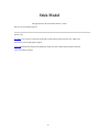
Stick Model
This page describes the stick model and how it works.
Below is the Stick Model Diagram,
Source Code:
ph_stick.cC file written in S-Function format that reads the analog signals from the stick, rudder, and
throttle then converts that signal to digital.
stick.mdlSimulink block diagram that graphically displays the pilot's input and the produced output in
terms of nominal percentage.
50
Instrument Model
This page describes the instrument model and how it works.
Below is the Instrument Model Diagram,
Source Code:
alinst.cC file written in S-Function format that receives the digital inputs from the simulation then converts
the value to an Analog signal to drive the instruments.
stick.mdlSimulink block diagram that graphically displays the instrument output for each of the instruments
based on the digital input.
51
SixDOF Model
This page describes the SixDOF model and how it works.
The SixDOF Model treats the aircraft like a point mass. It converts the Forces and Moments and Control
Inputs generated by the aircraft to compute the aircraft's position and orientation. The term 6 Degress of
Freedom refers to the aircrafts translational and rotational positions, x,y,z, and Psi, Theta, Phi.
Source Code:
sixdof1.c C file written in S-Function format that computes the SIXDOF position.
SIXDOF.mdl Simulink block diagram that graphically displays the inputs and outputs to the C-code.
navion.tsf A standard data file, SAD file, that contains the aircraft stability derivitives.
52
Standard Atmosphere Model
This page describes the Standard Atmosphere model and how it works.
The Standard Atmoshere Model receives the aircraft's current altitude and computes the density, pressure,
temperature, and speed of sound at that altitude.
Source Code:
std_atm.c C file written in S-Function format that computes the pressure, density, temperature, and speed of
sound for any given altitude.
Atmosphere.mdl Simulink block diagram that graphically displays the inputs and outputs to the C-code.
53
Standard Atmosphere Model
This page describes the Standard Atmosphere model and how it works.
The Standard Atmoshere Model receives the aircraft's current altitude and computes the density, pressure,
temperature, and speed of sound at that altitude.
Source Code:
std_atm.c C file written in S-Function format that computes the pressure, density, temperature, and speed of
sound for any given altitude.
Atmosphere.mdl Simulink block diagram that graphically displays the inputs and outputs to the C-code.
54
Engine Model
This page describes the Engine model and how it works. The Engine Model calculates the thrust generated
by each engine based on the engine type, static sea level thrust, and the density ratio. The 5 engines that are
modeled are a propeller piston engine, turboprop, hi-bypass, and a turbojet with and without afterburner
capability.
The Engine Model consists of a Spool Up / Spool Down Model which gives the engine a realistic feel by
adding a .25 second time delay on spool up and a .5 second time delay when spooling down.
Included is the work performed by the Spring 2000 Aero 320 class who developed the Engine Model,
Tested it, Calibrated the Throttle as well as the Instruments. Engine Model Simulation
Below is the Engine Model Diagram,
Source Code:
Spring AERO 320 class Engine Model Simulation
engine_mod.cC file written in S-Function format that receives the throttle inputs from the stick model, then
calculates the engine model variables.
engine.mdlSimulink block diagram that graphically displays the engine model outputs based on throttle
position. Embedded is the spooling model.
spool.cC file written in S-Function format that computes the time delay for the throttles based on whether
they are spooling up or spooling down.
spooltst.mdlSimulink block diagram that graphically displays the spool model outputs based on throttle
position.
55
Tutorial #1: Times Two Tutorial
This tutorial introduces the user on how to link Matlab Simulink block diagrams with C-source code.
Introduction:
Matlab links source code to simulink diagrams using the S-Function. The S-Function is found in the
simulink library under the non-linear toolbox. Refer to the simulink model below (xtwo.mdl) to see how
the S-Function is used within a Simulink block diagram. Notice that the input goes into the S-Function and
the output comes out of the S-Function (simple right).
The diagram is simple however the code is not. Look at the C-File source code shown below (timestwo.c).
For a simple program that reads in one value, multiplies that value by two, then returns it becomes quite
complex. For now, don't get too discouraged about figuring out the code. The objective of this tutorial is to
learn how to link simulink block diagrams with C-Source code. The next tutorial is to actually understand
the code.
Steps:
When performing these steps, don't just copy the model but actually draw the simulink diagrams.
Remember this is a tutorial for your own benefit.
1. Create a directory for you to practice your tutorials in.
2. Create a simulink block diagram similiar to xtwo.mdl.
3. Name the S-Function. Right click on the S-function to get the parameters window. NOTE: Make sure the
S-Function has a different name then the simulink model.
4. Copy the timestwo.c to your tutorial directory. Look over the code and become familiar with it's
structure. Find where the S-Function is defined. Make sure that this name is the same as the one that you
used earlier in step 3. Find where the input is multiplied by two then returned.
56
5. Create the .dll. dll's stand for dynamic linked libraries. You'll find them everywhere on any computer.
Basically, a .dll links code to other files. For our case we need to link the simulink diagram to the source
code. Here's how to create a dll.
5a. Open Matlab. Go to directory in Step 1. NOTE: Model and source code do not have to be in the same
directory, but for this case it's better to have them in the same directory. Type "pwd" at the command
prompt to make sure the path is set to your working directory.
5b. At the command prompt type: mex -setup. This will bring up the DOS window.
5c. Select Watcom C/C++ compiler, version 10.6, location c:/watcom, [y] or return.
5d. Type "cmex" and the name of the C-source file that you wish to create the dll from. Make sure that the
directory shown at the command prompt is where the source code file is located. Then type exit to close the
DOS window.
ie. D:\Projects\Test> cmex timestwo.c
6. Now you've linked the simulink block diagram to the source file and your ready to run the simulation.
Source Code:
timestwo.c C file written in S-Function format that multiplies the input by 2. (Pretty hefty file for a simple
function)
xtwo.mdl Simulink block diagram that graphically displays the user's input and the produced output.
57
Tutorial #2: Speed of Sound Tutorial
This tutorial introduces the user on how to link Matlab Simulink block diagrams with multiple inputs and
outputs to C-source code, as well as becoming familiar with the S-Function format.
Introduction:
This tutorial is similiar to Tutorial #1 except now we are going to have multiple inputs and outputs for the
S-Function. The goal of this tutorial is to create a model that reads 4 inputs: gamma, R, Temp, and velocity;
then calculates the speed of sound and Mach number and displays them in the Simulink window. To do this
you will need to develop a subsystem (seeMach.mdl).
A subsystem is necessary whenever there are multiple inputs and outputs or when you are developing a
model. This allows the entire simulation diagram to become less cluttered and easier to follow. The
subsystem icon can be found in the Simulink library under connections. Basically, when you doubleclick
on a subsystem, it gives you a new Simulink window.
An S-Function that has multiple outputs and inputs needs a Multiplexer (MUX) and DeMultiplexer
(DEMUX). The MUX and DEMUX icons can be found in the simulink library under connections. This
basically allows the input and output to be in array form. Each of the inputs and outputs must be assigned to
a port. You can specify the number of ports by right clicking on the MUX and DEMUX and selecting
parameters. The input and output ports can be found in the connections toolbox as well.
Once we have the model set up, we need to develop the S-Function. This time, instead of copying the code
directly, you're going to write each line of the code and achieve a simple understanding of the S-Function
format. Look at speed_sound.c. This file is a little cleaner in comparison to timestwo.c but is still of the
same form. Go over the code, and look at the comments. The comments show you where variables are
declared, where the number of inputs and outputs are determined, where the inputs and output arrays are
filled, and where the computation occurs.
Once you have finished writing the code, repeat the process you did in tutorial #1 to generate the dll
necessary for run time. Other important files to look over to try to understand the S-Function format
are:simstruc.h , simulink.c , and sfuntmpl.doc .
58
Source Code:
speed_sound.cC file written in S-Function format that reads in 4 inputs (Gamma, R, Temp, Velocity) and
computes 2 outputs (Speed of Sound and Mach Number).
Mach.mdlSimulink block diagram that graphically displays the user's input and the produced output. This
model is more complex then the XTwo model since a subsystem is required for multiple inputs and outputs.
simstruc.hSimulink header file that describes the included file necessary for the S-Function. Good reference
to see what functions could be added, and the structure necessary for those functions. Look at the
comments and the structure.
simulink.cAnother inprotant Simulink header file that describes another included file necessary for the
MEX Function. Good reference to see what is required for the MEX function. Again, look at the comments
and the structure.
sfuntmpl.docExcellent source of documentation for understanding the S-Function format. Notice that it is
referred to in all the source code files.
59
B.1 Engine_Mod.c
/* S-function engine_mod
* MODULE: engine_mod.c
* AUTHOR(S): Robert A. Barger, Dieter Pestal, Dan Salluce
* DATE:
May 11, 2000
* Copyright (c) ALL RIGHTS RESERVED
*
* REVISION HISTORY:
* REV AUTHOR DATE
DESCRIPTION
* 0 rab 5-11-00 Creation of code and Simulink Model
*
* This C-file S-function simulates the engine model based on the current throttle
*position as well as the current state that the engine is in. This engine model allows *four
different types of engines to be modeled: (1) - Propeller piston engine, (2) - *Turboprop,
(3) - Hi Bypass, (4) - Turbojet with Afterburner or without. The thrust
* based on altitude, fuel flow, nozzle position, RPM, and engine temp are calculated.
*
* Inputs:
*
RFuelCap
*
LFuelCap
*
EngType
*
Np - Prop Efficiency
*
RThrottle, %
60
*
LThrottle, %
*
Tsl, lbs
*
TSFCslNAB, (non-Afterburning TSFC - Sea Level)
*
TSFCslAB, (Afterburning TSFC - Sea Level)
*
rho,
*
a, (acoustic speed at altitude)
*
Vtrue, knots
*
* Outputs:
*
RFuelFlo, lbs of fuel/hr
*
LFuelFlo, lbs of fuelhr
*
RThrust, lbf
*
LThrust, lbf
*
RNoz, %
*
LNoz, %
*
RRPM, %
*
LRPM, %
*
RTemp, 0C
*
LTemp, 0C
*
* Cal Poly San Luis Obispo
* San Luis Obispo, CA
* See simulink/src/sfuntmpl.doc
61
* Also see Pheagle_HTML
*
* Copyright (c) 1990-1998 by The MathWorks, Inc. All Rights Reserved.
* $Revision: 1.3 $
*/
//Define the S-Function Name the same as in Simulink model.
#define S_FUNCTION_NAME engine_mod
//Define the S-Function Level to be 2 for Models
#define S_FUNCTION_LEVEL 2
//This header file is necessary for Simulink data structure. It is highly
//suggested to look at this file to see the structure of the S-Function.
#include "simstruc.h"
//Include any C++ header files or other files needed for syntax or class definition.
#include <stdio.h>
#include <math.h>
//Declare local input and output varaible names.
//Inputs:
float RFuelCap, LFuelCap, Np, RThrottle, LThrottle, Tsl;
62
float TSFCslNAB, TSFCslAB, rho, a, Vtrue;
int EngType, NumEng;
//Outputs:
float RFuelFlo, LFuelFlo, RThrust, LThrust, RRPM, LRPM, RNoz, LNoz, RTemp,
LTemp;
void Calculate( );
/* Function: mdlInitializeSizes ======================================
* Abstract:
* Setup sizes of the various vectors.
*/
static void mdlInitializeSizes(SimStruct *S)
{
ssSetNumSFcnParams(S, 0);
if (ssGetNumSFcnParams(S) != ssGetSFcnParamsCount(S)) {
return; /* Parameter mismatch will be reported by Simulink */
}
//This section sets up the number of inputs.
if (!ssSetNumInputPorts(S, 1)) return;
63
ssSetInputPortWidth(S, 0, 13);
//12 is the number of inputs.
ssSetInputPortDirectFeedThrough(S, 0, 1);
if (!ssSetNumOutputPorts(S,1)) return;
ssSetOutputPortWidth(S, 0, 10);
//10 is the number of outputs
ssSetNumSampleTimes(S, 1);
/* Take care when specifying exception free code - see sfuntmpl.doc */
ssSetOptions(S, SS_OPTION_EXCEPTION_FREE_CODE);
}
/* Function: mdlInitializeSampleTimes ================================
* Abstract:
*
Specifiy that we inherit our sample time from the driving block.
*/
static void mdlInitializeSampleTimes(SimStruct *S)
{
ssSetSampleTime(S, 0, INHERITED_SAMPLE_TIME);
ssSetOffsetTime(S, 0, 0.0);}
#define MDL_START
#if defined(MDL_START)
/* Function: mdlstart
64
* Initialize the state variables
*/
static void mdlStart(SimStruct *S)
{
//This is where you add code for the first time the simulation starts.
//For this simple file there is no need for any code in this section.
}
#endif /* MDL_START */
/* Function: mdlOutputs ===========================================
* Abstract: This section assigns the input variables to pointers in the u array,
*
and assigns the outputs to the y array. The speed of sound and Mach
*
Number is calculated in the Calculate() function.
*
* Inputs:
*
RFuelCap=*uPtrs[0];
*
LFuelCap=*uPtrs[1];
*
EngType=*uPtrs[2];
*
Np=*uPtrs[3];
*
RThrottle=*uPtrs[4];
*
LThrottle=*uPtrs[5];
*
Tsl=*uPtrs[6];
*
TSFCslNAB=*uPtrs[7];
65
*
TSFCslAB=*uPtrs[8];
*
rho=*uPtrs[9];
*
a=*uPtrs[10];
*
Vtrue=*uPtrs[11];
* Outputs:
*
y[0]=RFuelFlo;
*
y[1]=LFuelFlo;
*
y[2]=RThrust;
*
y[3]=LThrust;
*
y[4]=RNoz;
*
y[5]=LNoz;
*
y[6]=RRPM;
*
y[7]=LRPM;
*
y[8]=RTemp;
*
y[9]=LTemp;
*/
static void mdlOutputs(SimStruct *S, int_T tid)
{
InputRealPtrsType uPtrs = ssGetInputPortRealSignalPtrs(S,0);
real_T
*y = ssGetOutputPortRealSignal(S,0);
//Read in the Inputs:
RFuelCap=*uPtrs[0];
66
LFuelCap=*uPtrs[1];
EngType=*uPtrs[2];
Np=*uPtrs[3];
RThrottle=*uPtrs[4];
LThrottle=*uPtrs[5];
Tsl=*uPtrs[6];
TSFCslNAB=*uPtrs[7];
TSFCslAB=*uPtrs[8];
rho=*uPtrs[9];
a=*uPtrs[10];
Vtrue=*uPtrs[11];
NumEng=*uPtrs[12];
//Calculate the Engine States:
Calculate();
//Assign the Outputs:
y[0]=RFuelFlo;
y[1]=LFuelFlo;
y[2]=RThrust;
y[3]=LThrust;
y[4]=RNoz;
y[5]=LNoz;
67
y[6]=RRPM;
y[7]=LRPM;
y[8]=RTemp;
y[9]=LTemp;
}// end model outputs
void Calculate( ){
const float rhosl = 0.002377; // - slug/ft3
float asl=1116.2;
//-ft/s
float Thrust;
float TSFC;
float FuelFlow;
//Propeller Engine: Engine Type = 1
if (EngType == 1){
Thrust=(Tsl*550)*(rho/rhosl)*(Np/(Vtrue*1.69)); //Tsl - shp
if (NumEng == 1){
RThrust=0.5*RThrottle*Thrust;
LThrust=0.5*LThrottle*Thrust;
//printf("RThrust1-1: %i\n",RThrust);
//printf("LThrust1-1: %i\n",LThrust);
}
else if (NumEng == 2){
68
RThrust=RThrottle*Thrust;
LThrust=LThrottle*Thrust;
//printf("RThrust1-2: %i\n",RThrust);
//printf("LThrust1-2: %i\n",LThrust);
}
}
//Turboprop Engine: Engine Type = 2
if (EngType == 2){
Thrust=(Tsl*550)*(rho/rhosl)*(Np/(Vtrue*1.69)); //Tsl - eshp
if (NumEng == 1){
RThrust=0.5*RThrottle*Thrust;
LThrust=0.5*RThrottle*Thrust;
//printf("RThrust2-1: %i\n",RThrust);
//printf("LThrust2-1: %i\n",LThrust);
}
else{
RThrust=RThrottle*Thrust;
LThrust=LThrottle*Thrust;
//printf("RThrust2-2: %i\n",RThrust);
//printf("LThrust2-2: %i\n",LThrust);
}
}
69
//High By-pass Engine: Engine Type = 3
if (EngType == 3){
Thrust=(0.1/(Vtrue*1.69/a))*Tsl*(rho/rhosl); //Tsl - lbs
if (NumEng == 1){
RThrust=0.5*RThrottle*Thrust;
LThrust=0.5*LThrottle*Thrust;
//printf("RThrust3-1: %i\n",RThrust);
//printf("LThrust3-1: %i\n",LThrust);
}
else{
RThrust=RThrottle*Thrust;
LThrust=LThrottle*Thrust;
//printf("RThrust3-2: %i\n",RThrust);
//printf("LThrust3-2: %i\n",LThrust);
}
}
//Non - Afterburning Jet Engine: Engine Type = 4
if (EngType == 4){
Thrust=Tsl*(rho/rhosl); //Tsl - lbs
if (NumEng == 1){
RThrust=0.5*RThrottle*Thrust;
70
LThrust=0.5*LThrottle*Thrust;
//printf("RThrust4-1: %i\n",RThrust);
//printf("LThrust4-1: %i\n",LThrust);
}
else{
RThrust=RThrottle*Thrust;
LThrust=LThrottle*Thrust;
//printf("RThrust4-2: %i\n",RThrust);
//printf("LThrust4-2: %i\n",LThrust);
}
}
//Afterburning Jet Engine: Engine Type = 5
if (EngType == 5){
Thrust=Tsl*(rho/rhosl)*(1+0.7*(Vtrue*1.69/a)); //Tsl - lbs
if (NumEng == 1){
RThrust=0.5*RThrottle*Thrust;
LThrust=0.5*LThrottle*Thrust;
//printf("RThrust5-1: %i\n",RThrust);
//printf("LThrust5-1: %i\n",LThrust);
}
else{
RThrust=RThrottle*Thrust;
71
LThrust=LThrottle*Thrust;
//printf("RThrust5-2: %i\n",RThrust);
//printf("LThrust5-2: %i\n",LThrust);
}
}//End Thrust Calculation
//Calculate fuel flow
if (EngType == 5){
//Afterburning engine
if (RThrottle > 0.65){ //Afterburner engaged
TSFC = TSFCslAB*(a/asl);
FuelFlow = TSFC*(RThrust);
RFuelFlo = FuelFlow;}
else{
TSFC = TSFCslNAB*(a/asl);
FuelFlow = TSFC*(RThrust);
RFuelFlo = FuelFlow;}
if (LThrottle >0.65){ //Afterburner engaged
TSFC = TSFCslAB*(a/asl);
FuelFlow = TSFC*(LThrust);
LFuelFlo = FuelFlow;}
else{
72
TSFC = TSFCslNAB*(a/asl);
FuelFlow = TSFC*(LThrust);
LFuelFlo = FuelFlow;}
} //non afterburning engine
else{
TSFC = TSFCslNAB*(a/asl);
FuelFlow = TSFC*(RThrust);
RFuelFlo = FuelFlow;
TSFC = TSFCslNAB*(a/asl);
FuelFlow = TSFC*(LThrust);
LFuelFlo = FuelFlow;
} //end TSFC calc
//Calculate the Right Engine RPM.
RRPM=RThrottle*100;
//Calculate the Left Engine RPM.
LRPM=LThrottle*100;
//Calculate the Right Engine Nozzle Position.
RNoz=RThrottle*100;
73
//Calculate the Left Engine Nozzle Position.
LNoz=LThrottle*100;
//Calculate the Right Engine Temp.
RTemp=(RThrottle*1400);
//Calculate the Left Engine Temp.
LTemp=(LThrottle*1400);
return;
} //end calculate
/* Function: mdlTerminate =========================================
* Abstract:
* No termination needed, but we are required to have this routine. */
static void mdlTerminate(SimStruct *S)
{
}
#ifdef MATLAB_MEX_FILE
#include "simulink.c"
/* Is this file being compiled as a MEX-file? */
/* MEX-file interface mechanism */
#else
74
#include "cg_sfun.h"
/* Code generation registration function */
#endif
75
B.2 Spool.c
/*********************************************************************
MODULE:
spool.c
* AUTHOR(S): Robert A. Barger, Michael Ortner, Jeff Doll
* DATE:
September 25, 1998
* Copyright (c) ALL RIGHTS RESERVED
* Cal Poly San Luis Obispo 1998
*
* REVISION HISTORY:
* REV AUTHOR DATE
DESCRIPTION
* 0 rab 5-11-oo Creation of code and Simulink Model
*
* S-mex: See simulink/src/sfuntmpl.doc
* S-mex Copyright (c) 1990-1998 by The MathWorks, Inc. All Rights Reserved.
* $Revision: 1.3
*
* This S-function block Reads the commanded throttle position and determines
* whether the engines are spooling up or spooling down. The program keeps track
* of the last position and if the difference is positive then the engine is
* spooling down else it is spooling up. The spool up time delay was set to 0.5 sec
* and the spool down time delay was set to 0.25 sec.
********************************************************************/
#define S_FUNCTION_NAME spool
76
#define S_FUNCTION_LEVEL 2
#include "simstruc.h"
#include <dos.h>
//#include <bios.h>
#include <math.h>
#include <stdlib.h>
#include <string.h>
#include <conio.h>
#include <math.h>
#include <stdio.h>
double oldVals[2];
double LThrottle, RThrottle;
int LTauDN=0;
int RTauDN=0;
/* Function: mdlInitializeSizes=======================================
* Abstract:
* Setup sizes of the various vectors. */
static void mdlInitializeSizes(SimStruct *S)
77
{
ssSetNumSFcnParams(S, 0);
if (ssGetNumSFcnParams(S) != ssGetSFcnParamsCount(S)) {
return; /* Parameter mismatch will be reported by Simulink */
}
//is section sets up the number of inputs.
if (!ssSetNumInputPorts(S, 1)) return;
ssSetInputPortWidth(S, 0, 2);
//4 is the number of inputs.
ssSetInputPortDirectFeedThrough(S, 0, 1);
if (!ssSetNumOutputPorts(S,1)) return;
ssSetOutputPortWidth(S, 0, 4);
//2 Number of outputs
/* Stick, rudder, and throttles */
ssSetNumSampleTimes(S, 1);
/* Take care when specifying exception free code - see sfuntmpl.doc */
ssSetOptions(S, SS_OPTION_EXCEPTION_FREE_CODE);
}
/* Function: mdlInitializeSampleTimes ================================
78
* Abstract:
*
Specifiy that we inherit our sample time from the driving block.
*/
static void mdlInitializeSampleTimes(SimStruct *S)
{
ssSetSampleTime(S, 0, INHERITED_SAMPLE_TIME);
ssSetOffsetTime(S, 0, 0.0);
}
#define MDL_START /* Change to #undef to remove function */
#if defined(MDL_START)
/* Function: mdlStart ======================================
* Abstract:
*
Initialize the da cards.*/
static void mdlStart(SimStruct *S)
{
}
#endif /* MDL_START */
#define MDL_INITIALIZE_CONDITIONS /* Change to #undef to remove function */
#if defined(MDL_INITIALIZE_CONDITIONS)
/* Function: mdlInitializeConditions ==================================
* Abstract:
79
*
Initialize the state. Note, that if this S-function is placed
*
with in an enabled subsystem which is configured to reset states,
*
this routine will be called during the reset of the states.*/
static void mdlInitializeConditions(SimStruct *S)
{
}
#endif /* MDL_INITIALIZE_CONDITIONS */
/* Function: mdlOutputs===========================================
* Abstract:
*
simply passes states y[n] = x[n]
*/
static void mdlOutputs(SimStruct *S, int_T tid)
{
InputRealPtrsType uPtrs = ssGetInputPortRealSignalPtrs(S,0);
real_T
*y = ssGetOutputPortRealSignal(S,0);
//read in inputs
LThrottle=*uPtrs[0];
RThrottle=*uPtrs[1];
if ((oldVals[0]-LThrottle)>0)
LTauDN = 1; //.25 second time delay on spool down
80
else
LTauDN = 0;
//.50 second time delay on spool up
if ((oldVals[1]-RThrottle)>0)
RTauDN = 1; //.25 second time delay on spool down
else
RTauDN = 0;
//.50 second time delay on spool up
y[0] = LThrottle;
y[1] = RThrottle;
y[2] = LTauDN;
y[3] = RTauDN;
oldVals[0]=LThrottle;
oldVals[1]=RThrottle;
}
#define MDL_UPDATE /* Change to #undef to remove function */
#if defined(MDL_UPDATE)
/* Function: mdlUpdate ===========================================
* Abstract:
*
This function is called once for every major integration time step.
* Discrete states are typically updated here, but this function is useful
81
* for performing any tasks that should only take place once per
*
integration step.
*/
static void mdlUpdate(SimStruct *S, int_T tid)
{
}
#endif /* MDL_UPDATE */
#define MDL_DERIVATIVES /* Change to #undef to remove function */
#if defined(MDL_DERIVATIVES)
/* Function: mdlDerivatives =======================================
*/
static void mdlDerivatives(SimStruct *S)
{
}
#endif /* MDL_DERIVATIVES */
/* Function: mdlTerminate==========================================
* Abstract:
* No termination needed, but we are required to have this routine.
*/
static void mdlTerminate(SimStruct *S)
{
82
}
#ifdef MATLAB_MEX_FILE
#include "simulink.c"
/* Is this file being compiled as a MEX-file? */
/* MEX-file interface mechanism */
#else
#include "cg_sfun.h"
/* Code generation registration function */
#endif
83
B.3 ILS_Model.c
/* S-function ils_model
* MODULE:
ils_model.c
* AUTHOR(S): Robert A. Barger, Edwin Casco, Paul Patangui
* DATE:
May 18, 2000
*
* Copyright (c) ALL RIGHTS RESERVED
*
* REVISION HISTORY:
* REV AUTHOR DATE
DESCRIPTION
* 0 rab 5-18-00 Creation of code and Simulink Model
*
* This C-file S-function simulates an ILS beacon located at the end
* of the runway. The required inputs are the aircraft's position as
* well as the airport's location and runway heading. The CDI and CDVert
* are the angles off the runway centerline. They are the same angle just
* at different scales. The CdHor angle is the approach glide slope angle.
* In order to be on Glideslope, this angle must be -2.5 degrees.
*
* Inputs:
*
ACX - Aircraft X position,ft
*
ACY - Aircraft Y position,ft
*
ACZ - Aircraft Z position,ft
*
ACU - Aircraft U, ft
84
*
ACV - Aircraft Y position,ft
*
ACW - Aircraft Z position,ft
*
APX - Airport X position, ft
*
APY - Airport Y position, ft
*
APZ - Airport Z position, ft
*
APpsi - Airport Heading, degrees
*
* Outputs:
*
CDI - Course Deviation Indicator, deg +/-10 scale
*
CDVert - Course Deviation Vertical Indicator, deg +/-2.5 scale
*
CDHor - Course Deviation Horizontal Indicator, deg +/-2.5 scale
*
* Edwin Casco
* Paul Patangui
* Robert Barger
* Cal Poly San Luis Obispo
* San Luis Obispo, CA
*
* See simulink/src/sfuntmpl.doc
* Also see Pheagle_HTML
*
* Copyright (c) 1990-1998 by The MathWorks, Inc. All Rights Reserved.
* Revision: 1.3*/
//Define the S-Function Name the same as in Simulink model.
85
#define S_FUNCTION_NAME ils_model
//Define the S-Function Level to be 2 for Models
#define S_FUNCTION_LEVEL 2
//This header file is necessary for Simulink data structure. It is highly
//suggested to look at this file to see the structure of the S-Function.
#include "simstruc.h"
//Include any C++ header files or other files needed for syntax or class definition.
#include <stdio.h>
#include <math.h>
//Declare local input and output varaible names.
//Inputs:
double ACX, ACY, ACZ, ACU, ACV, ACW, APX, APY, APZ, APpsi;
//Outputs:
double CDI, CDVert, CDHor;
void Calculate( );
/* Function: mdlInitializeSizes ======================================
86
* Abstract:
* Setup sizes of the various vectors.
*/
static void mdlInitializeSizes(SimStruct *S)
{
ssSetNumSFcnParams(S, 0);
if (ssGetNumSFcnParams(S) != ssGetSFcnParamsCount(S)) {
return; /* Parameter mismatch will be reported by Simulink */
}
//This section sets up the number of inputs.
if (!ssSetNumInputPorts(S, 1)) return;
ssSetInputPortWidth(S, 0, 10);
//10 is the number of inputs.
ssSetInputPortDirectFeedThrough(S, 0, 1);
if (!ssSetNumOutputPorts(S,1)) return;
ssSetOutputPortWidth(S, 0, 3);
//3 is the number of outputs
ssSetNumSampleTimes(S, 1);
/* Take care when specifying exception free code - see sfuntmpl.doc */
ssSetOptions(S, SS_OPTION_EXCEPTION_FREE_CODE);
}
87
/* Function: mdlInitializeSampleTimes ================================
* Abstract:
*
Specifiy that we inherit our sample time from the driving block.
*/
static void mdlInitializeSampleTimes(SimStruct *S)
{
ssSetSampleTime(S, 0, INHERITED_SAMPLE_TIME);
ssSetOffsetTime(S, 0, 0.0);
}
#define MDL_START
#if defined(MDL_START)
/* Function: mdlstart
* Initialize the state variables
*/
static void mdlStart(SimStruct *S)
{
//This is where you add code for the first time the simulation starts.
//For this simple file there is no need for any code in this section.
}
#endif /* MDL_START */
88
/* Function: mdlOutputs==========================================
* Abstract: This section assigns the input variables to pointers in the u array,
*
and assigns the outputs to the y array. The deviation angles are
*
calculated in the Calculate() function.
*
* Inputs:
*
ACX=*uPtrs[0];
*
ACY=*uPtrs[1];
*
ACZ=*uPtrs[2];
*
ACU=*uPtrs[3];
*
ACV=*uPtrs[4];
*
ACW=*uPtrs[5];
*
APX=*uPtrs[6];
*
APY=*uPtrs[7];
*
APZ=*uPtrs[8];
*
APpsi=*uPtrs[9];
*
* Outputs:
*
y[0]=CDI;
*
y[1]=CDVert;
*
y[2]=CDHor;
*/
static void mdlOutputs(SimStruct *S, int_T tid)
89
{
InputRealPtrsType uPtrs = ssGetInputPortRealSignalPtrs(S,0);
real_T
*y = ssGetOutputPortRealSignal(S,0);
//Read in the Inputs:
ACX=*uPtrs[0];
ACY=*uPtrs[1];
ACZ=*uPtrs[2];
ACU=*uPtrs[3];
ACV=*uPtrs[4];
ACW=*uPtrs[5];
APX=*uPtrs[6];
APY=*uPtrs[7];
APZ=*uPtrs[8];
APpsi=*uPtrs[9];
//Calculate the Deviation Angles:
Calculate();
//Assign the Outputs:
y[0]=CDI;
y[1]=CDVert;
y[2]=CDHor;
90
}
void Calculate( ){
const double GlideSlope=-2.5; //Define the Glide Slope Angle
const float pi = 3.14159;
double Theta1=0; //Angle from Horizontal.
double Theta2=0; //Supplement of Theta1.
double Theta3=0; //From Horizontal to runway centerline.
double Theta4=0; //Angle from Horizontal to airport.
double x=0;
//X distance between aircraft and airport.
double y=0;
//Y distance between aircraft and airport.
double z=0;
//Z distance between aircraft and airport.
double a=0;
//Arc Length of CDVert
double r=0;
//Radial distance from airport to aircraft.
double lambda=0;
//Calculate Theta for CDI and CDVert
x = -(ACX-APX);
y = ACY-APY;
z = ACZ-APZ;
r = sqrt(x*x+y*y);
Theta1 = atan(y/x);
91
Theta2 = pi+Theta1;
Theta3 = -((2*pi)-(APpsi*pi/180));
Theta4 = atan(z/x);
lambda = (90*pi/180)-(Theta1-Theta3);
a=cos(lambda)*r;
CDVert= 57.3*(sin(a/r));
CDI=CDVert;
//Same angle, different scale
//Calculate CDHor
CDHor = 57.3*(Theta4-(GlideSlope*pi/180));
return;
}
/* Function: mdlTerminate =========================================
* Abstract:
* No termination needed, but we are required to have this routine.
*/
static void mdlTerminate(SimStruct *S)
{
}
92
#ifdef MATLAB_MEX_FILE
#include "simulink.c"
/* Is this file being compiled as a MEX-file? */
/* MEX-file interface mechanism */
#else
#include "cg_sfun.h"
/* Code generation registration function */
#endif
93
B.4 Server.c
/********************************************************************
* MODULE: server.c
* AUTHOR(S): Robert A. Barger/ Jon Tonkyro
* DATE:
May 8, 2000
*
* Copyright (c) ALL RIGHTS RESERVED
*
* REVISION HISTORY:
* REV AUTHOR
* 0 JT
* 1 RAB
DATE
DESCRIPTION
5-05-00 Creation into C++ Format & Tested
5-08-00 Creation into S-Function Format
*
* S-mex: See simulink/src/sfuntmpl.doc
*
* Copyright (c) 1990-1998 by The MathWorks, Inc. All Rights Reserved.
* $Revision: 1.3
*
* This S-function block sends the position and orientation of the aircraft to
* the graphics client computers Eagle, Pheagle, and Phantom. This module acts
* as a server (Spiegel) to the other 3 clients. Slave.exe must be run on the
* other 3 clients as well as their batch files. The server sends a struct to
* the clients which can be modified to send more additional information. Different
94
* command line arguments can be added to Slave.exe to run different terrain
* databases, set the cloud layer, etc.
********************************************************************/
#define S_FUNCTION_NAME server
#define S_FUNCTION_LEVEL 2
#include "simstruc.h"
#include <dos.h>
#include <math.h>
#include <stdlib.h>
#include <string.h>
#include <conio.h>
#include <stdio.h>
//for Winsockets
#include <winsock2.h>
#include "server.h"
#define Service_Port 5001
#define BUFFER_SIZE 56
//declare variables
95
struct sockaddr_in you;
// the outgoing socket struct
SOCKET server_socket = 0;
// socket descriptor for the server socket
SOCKET client_socket = 0;
// socket descriptor for the client socket
int message_len = 0;
// length of the received message
struct Host_data host_data;
float x=1, y=2, z=3, psi=4, theta=5, phi=6;
char buf[BUFFER_SIZE];
// buffer for receiving from remote
int len=0;
/* Function: mdlInitializeSizes =====================================
* Abstract:
* Setup sizes of the various vectors.
*/
static void mdlInitializeSizes(SimStruct *S)
{
ssSetNumSFcnParams(S, 0);
if (ssGetNumSFcnParams(S) != ssGetSFcnParamsCount(S)) {
return; /* Parameter mismatch will be reported by Simulink */
}
if (!ssSetNumInputPorts(S, 1)) return;
ssSetInputPortWidth(S, 0, 6);
//x,y,z,psi,theta,phi
ssSetInputPortDirectFeedThrough(S, 0, 1);
96
if (!ssSetNumOutputPorts(S,0)) return;
/*
ssSetOutputPortWidth(S, 0, 1); */ //no outputs
ssSetNumSampleTimes(S, 1);
/* Take care when specifying exception free code - see sfuntmpl.doc */
ssSetOptions(S, SS_OPTION_EXCEPTION_FREE_CODE);
len=sizeof( struct sockaddr_in );
}
/* Function: mdlInitializeSampleTimes ================================
* Abstract:
*
Specifiy that we inherit our sample time from the driving block.
*/
static void mdlInitializeSampleTimes(SimStruct *S)
{
ssSetSampleTime(S, 0, INHERITED_SAMPLE_TIME);
ssSetOffsetTime(S, 0, 0.0);
}
97
#define MDL_START
#if defined(MDL_START)
/* Function: mdlstart ========
*/
static void mdlStart(SimStruct *S)
{
int temp;
//setup winsock
WSADATA info;
WSAStartup(MAKEWORD(1,1), &info);
// create the server socket
server_socket = tcp_recv_setup();
//wait for the client to say something..get his address
temp = recvfrom(server_socket, buf, sizeof(buf), 0, (struct sockaddr *)&you, &len);
printf("received hello from center client\n");
}
#endif /* MDL_START */
/* Function: mdlOutputs======================================= */
98
static void mdlOutputs(SimStruct *S, int_T tid)
{
int n;
InputRealPtrsType uPtrs = ssGetInputPortRealSignalPtrs(S,0);
//set host_data, Open_GVS coordinate system is different than Simulation
host_data.ownpos.x = *uPtrs[1];
//aircrafts y position
host_data.ownpos.y = *uPtrs[2];
//aircrafts altitude
host_data.ownpos.z = *uPtrs[0];
//aircrafts x position
host_data.ownrot.x = *uPtrs[4];
//pitch
host_data.ownrot.y = *uPtrs[5];
//yaw
host_data.ownrot.z = *uPtrs[3];
//bank
host_data.quit=0;
//send host_data to client
memcpy(buf, &host_data, sizeof(host_data));
n = sendto(server_socket, buf, sizeof(host_data), 0, (struct sockaddr*)&you,
sizeof(struct sockaddr_in));
}
SOCKET tcp_recv_setup()
99
{
// This function sets the server socket. It lets the system
// determine the port number. The function returns the server
// socket number.
SOCKET srv_socket = 0;
struct sockaddr_in local;
int len = sizeof(local);
// socket address for local side
/* length of local address */
// create the socket
srv_socket=socket(AF_INET,SOCK_DGRAM,0);
// bind the socket to a port, let the system decide the number
local.sin_family = AF_INET;
/* internet family */
local.sin_addr.s_addr = INADDR_ANY; /* wild card machine address */
local.sin_port = Service_Port;
/* choose the port */
bind(srv_socket, (struct sockaddr *) &local, sizeof(local));
//bind the name (address)
to a port
return srv_socket;
}
/* Function: mdlTerminate =========================================
100
* Abstract:
* No termination needed, but we are required to have this routine.
*/
static void mdlTerminate(SimStruct *S)
{
}
#ifdef MATLAB_MEX_FILE
#include "simulink.c"
/* Is this file being compiled as a MEX-file? */
/* MEX-file interface mechanism */
#else
#include "cg_sfun.h"
/* Code generation registration function */
#endif
101
B.5 Server.h
/********************************************************************
* MODULE: server.h
* AUTHOR(S): Robert A. Barger/ Jon Tonkyro
* DATE:
May 8, 2000
*
* Copyright (c) ALL RIGHTS RESERVED
*
* REVISION HISTORY:
* REV AUTHOR
* 0 JT
DATE
DESCRIPTION
5-05-00 Creation into C++ Format & Tested
* 1 RAB
5-08-00 Creation into S-Function Format
********************************************************************/
typedef float G_Gfloat;
/* Double precision */
typedef int G_Boolean ;
typedef struct {
G_Gfloat x;
G_Gfloat y;
G_Gfloat z;
} G_Vector3;
/* General 3D vector */
102
#define G_Position G_Vector3
#define G_Rotation G_Vector3
struct Host_data{
/* --------- Continous data from host (sent every frame) -------------- */
G_Position
ownpos;
/* Ownship vehicle position */
G_Rotation ownrot;
/* Ownship vehicle rotation angles */
int quit;
/* 1 to QUIT now */
};
SOCKET tcp_recv_setup();
SOCKET tcp_listen(int server_socket, int back_log);
SOCKET tcp_send_setup(char * host_name, char * port);
103
B.6 Slave.c
/********************************************************************
* MODULE: slave.c
* AUTHOR(S): Robert A. Barger/ Jon Tonkyro
* DATE:
May 20, 2000
*
* Copyright (c) ALL RIGHTS RESERVED
*
* REVISION HISTORY:
*
* REV AUTHOR
DATE
DESCRIPTION
* 0 JT&RAB 5-20-00 Creation & Tested
*
* Description:
*
Communications software for opening a UDP connection
*
between the master process (running equations of motion, Spiegel)
*
and a slave process (running graphics, Phantom, Eagle, and Pheagle).
*
Additional command line arguments can be implemented to porduce cloud
*
layer effects, change database, etc.
*
********************************************************************/
#include <g_sys.h>
#include <g_consts.h>
104
#include <gv.h>
#include <gvu_isg.h>
#include <tmfbf.h>
#include "modhostdata.h"
/* External host control data */
#include "slave.h"
/* Slave side stuff */
#define SERVER "129.65.180.41" //Spiegel's IP Address
#define Service_Port 5001
//Pipe-Line Port
#define BUFSIZE 56
//Size of the struct we're sending
#define NUM_VEHICLES 2
/* Global */
struct Host_data host_data;
/* Data from the master */
/* Global through this module only */
static GV_Obi vobi[NUM_VEHICLES];
static struct sockaddr_in remote;
static char * buf;
static int bufsize;
static int len=0;
static SOCKET socket_num;
105
/********************************************************************
* path_init -*
Dummy module -- not needed by slave
********************************************************************/
void path_init( void )
{
}
/********************************************************************
* eom_init -*
Dummy module -- not needed by slave
********************************************************************/
int eom_init( GV_Geometry geoset, GV_Obi inst, GV_Obi terrain,
G_Position *pos_init, G_Rotation *rot_init, float speed_init )
{
(void) geoset ;
(void) inst ;
(void) terrain ;
(void) pos_init ;
(void) rot_init ;
(void) speed_init ;
return G_FAILURE;
106
}
/********************************************************************
* slave_init -*
Initialize the communications interface -- called once
*
by the slave to establish communications with the host
********************************************************************/
int slave_init( void )
{
int status = G_SUCCESS;
static char * sktNameServer = "slave" ;
static char * sktHostPeer = NULL ;
/* anybody */
GV_Obi cursor;
GV_Scene scene;
int temp;
float x=-1, y=-2, z=-3, psi=-4, theta=-5, phi=-6;
WSADATA info;
if(WSAStartup(MAKEWORD(1,1), &info)==SOCKET_ERROR)
{
fprintf( stdout, "slave_get_data: error reading from socket\n" );
return (G_FAILURE);
}
107
//create the socket
socket_num=socket(AF_INET,SOCK_DGRAM,0);
fprintf( stdout, "created socket: %i\n",socket_num);
remote.sin_family=AF_INET;
remote.sin_addr.s_addr=inet_addr(SERVER);
remote.sin_port = Service_Port;
if(socket_num<0)
{
exit(-1);
}
GV_obi_inq_by_name( "CURSOR", &cursor );
if( cursor )
GV_obi_set_state( cursor, G_OFF );
GV_chn_inq_scene( channel[0], &scene );
if( scene )
{
int vehicle;
for( vehicle=0; vehicle<NUM_VEHICLES; vehicle++)
{
/* By master-slave conventions, vehicles are named "P1", "P2", ... */
108
G_Name name;
sprintf( name, "P%d", vehicle+1 );
GV_obi_instance_by_name( name, &vobi[vehicle] );
GV_scn_add_object( scene, vobi[vehicle] );
if( vobi[vehicle] )
fprintf( stdout, "slave_init: instanced vehicle named %s\n", name );
}
}
fprintf( stdout, "slave_init: Sending hello to server\n");
temp=sendto(socket_num, "hello", 4, 0, (struct sockaddr*)&remote, sizeof(struct
sockaddr_in));
fprintf( stdout, "slave_init: Sent hello to server\n");
if(temp<0)
{
perror("didn't work");
exit(-1);
}
//init host_data struct
//set host_data
host_data.ownpos.x = x;
host_data.ownpos.y = y;
host_data.ownpos.z = z;
109
host_data.ownrot.x = psi;
host_data.ownrot.y = theta;
host_data.ownrot.z = phi;
bufsize = sizeof(host_data);
buf = (char *)malloc( sizeof(host_data));
fprintf( stdout, "bufsize: %i, ",bufsize );
return status;
}
/********************************************************************
* slave_get_data -*
Called once per frame by the slave to read the host data
*
and update its graphics as commanded
********************************************************************/
int slave_get_data( GV_Obi ownship )
{
int status = G_SUCCESS;
GV_Camera camera;
int message_len=0;
char cameraname[5];
110
/* Get the latest packet that has been broadcast from the master
(more than one could be backed up in the Ethernet queue) */
len=sizeof(struct sockaddr_in);
message_len=recvfrom(socket_num, buf, bufsize,0 ,(struct sockaddr *)&remote,
&len);
memcpy(&host_data, buf, sizeof(host_data));
if( message_len < 0 )
{
fprintf( stdout, "slave_get_data: error reading from socket\n" );
return (G_FAILURE);
}
strcpy( cameraname, "PILOT" );
GV_obi_set_position( ownship, &host_data.ownpos );
GV_obi_set_rotation( ownship, &host_data.ownrot );
GV_cam_inq_by_name( cameraname, &camera );
GV_chn_set_camera( channel[1], camera );
return status;
}
111
B.7 ModHostData.h
/********************************************************************
* MODULE: modhostdata.h
* AUTHOR(S): Robert A. Barger/ Jon Tonkyro
* DATE:
May 20, 2000
*
* Copyright (c) ALL RIGHTS RESERVED
*
* REVISION HISTORY:
* REV AUTHOR
DATE
DESCRIPTION
* 0 JT&RAB 5-20-00 Creation & Tested
********************************************************************/
#include <gv_types.h>
struct Host_data{
/* --------- Continous data from host (sent every frame) -------------- */
G_Position
ownpos; .................. /* Ownship vehicle position
*/
G_Rotation ownrot;
...................... /* Ownship vehicle rotation angles */
int quit;
.................................... /* 1 to QUIT now
};
112
*/
113