Download EMX User`s Manual

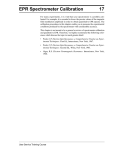
EPR Spectrometer Calibration
8
For many experiments, it is vital that your spectrometer is carefully calibrated. For example, it is essential to know the precise
values of the magnetic field modulation amplitude in order to
obtain quantitative EPR spectra. The calibration procedures in
this chapter enable you to measure the experimental conditions
produced by the spectrometer with considerable accuracy.
This chapter is not meant to be a general overview of spectrometer calibration and quantitative EPR. Therefore, we highly recommend the following references which discuss the topic in
much greater detail:
• Poole, C.P. Electron Spin Resonance, a Comprehensive Treatise on Experimental Techniques: First Ed., Interscience,
New York, 1967.
• Poole, C.P. Electron Spin Resonance, a Comprehensive Treatise on Experimental Techniques: Second Ed., Wiley, New
York, 1983.
• Alger, R.S. Electron Paramagnetic Resonance: Interscience,
New York, 1968.
EMX User’s Manual
Standard Samples
Standard Samples
8.1
Standard samples are useful for system performance tests, spectrometer calibration, and quantitative concentration measurements. Ideally the standard sample should contain stable, long
lived paramagnetic species, be easily prepared under consistent
and controlled methods, and should be fully characterized with
respect to all spectroscopic parameters such as relaxation times
and hyperfine and fine structure splittings. In addition, the resonance line should be narrow and preferably homogeneous.
Unfortunately, the universal standard sample has not been found.
Many standards have been suggested and each has its own particular merit. The standard samples supplied with every Bruker
spectrometer are discussed below.
DPPH (α, α‘ - diphenyl-ß-picryl hydrazyl)
8.1.1
DPPH serves as a reference both in the solid state and in the liquid state when dissolved in benzene or toluene/mineral oil. The
line width measured from the solid is subject to exchange narrowing and thus, varies from under 1 gauss to over 4 gauss,
depending on the solvent that was used for recrystallization. It
has a g factor of 2.0036 ± 0.0003. When dissolved in solution, a
quintet with unresolved hyperfine couplings is observed as the
spin exchange narrowing is reduced as the sample is diluted. A
small single crystal of DPPH is an ideal sample for calibrating
the phase and the field modulation amplitude of the signal channel of an EPR spectrometer. DPPH has been studied extensively
by:
• Möbius, K. and R. Biehl. Multiple Electron Resonance Spectroscopy: Plenum Press, 1979.
• Dalal, N.S., D.E. Kennedy, and C.A. McDowell. J. Chem.
Phys.: 59, 3403 (1979).
8-2
Standard Samples
• Hyde, H.S., R.C. Sweed, Jr., and G.H. Rist. J. Chem. Phys.:
51, 1404 (1969).
• Dalal, N.S., D.E. Kennedy, and C.A. McDowell. J. Chem.
Phys.: 61, 1989 (1974).
• Dalal, N.S., D.E.Kennedy, and C.A. McDowell. Chem. Phys.
Lett.: 30, 186 (1975).
Weak and Strong Pitch Samples
8.1.2
Pitch in KCl has emerged as a standard because of its long-lived
paramagnetic radicals and low dielectric loss. Because of the
long life of the radicals, it is unsurpassed as a test of spectrometer sensitivity. The pitch is added to a powder of KCl and the
mixture is carefully mechanically mixed to obtain a homogeneous sample. After mixing, the sample is heated, pumped and
sealed under vacuum. Pitch is generally prepared in two concentrations: strong pitch which is 0.11% pitch in KCl, and weak
pitch which is 0.0003% pitch in KCl.
To correct for variations in spin concentration, each weak pitch
sample is compared to a “standard” and assigned a correction
factor. The peak to peak line width is typically 1.7 G with a
g-factor of 2.0028. The size (very weak) of the signal renders
pitch ill suited for modulation amplitude calibration. The weak
pitch samples from Bruker Instruments have a nominal concentration of 1013 spins per centimeter. The samples are calibrated
and the correction factor is printed on the side of the tube. This
sample is prepared for the purpose of measuring instrument performance owing to its high stability, however, it is not meant as a
quantitative spin-counting standard.
EMX User’s Manual
8-3
Calibration of the Signal Channel
Calibration of the Signal Channel
8.2
You need to carefully calibrate your spectrometer’s signal channel reference phase and modulation amplitude in order to obtain
maximum sensitivity, minimum distortion, and quantitatively
reproducible measurements. The EMX027 in conjunction with
the WIN-EPR Acquisition software make this calibration easy to
perform. The results of the calibration are saved on disk for
future use. We recommend recalibration at least once a year to
ensure quantitative and reproducible results. Each cavity or resonator has its own individual calibration file, therefore, this procedure must be followed for each cavity.
Basic Theory
8.2.1
Calibration of the signal channel involves two separate yet interdependent procedures. The first procedure is to calibrate the
peak to peak modulation amplitude. For the sake of brevity,
modulation amplitude will be used in place of peak to peak modulation amplitude. The second procedure is to calibrate the phase
difference between the reference signal and the modulated EPR
signal. Because the calibration and adjustment of the modulation
amplitude can affect the phase difference, the first procedure is
performed first.
You calibrate the modulation amplitude by overmodulating a
narrow EPR signal. A crystal of DPPH, with a line width of
approximately 1 G, is a very good sample to use. When the modulation amplitude is large compared to the line width, the magnetic field modulation brings the sample into resonance before
and after the magnet has reached the field for resonance. This
results in a broadening and distortion of the EPR signal. (See
Figure 8-1.) In the limit of an infinitesimally narrow EPR signal, the peak to peak width of the first derivative EPR signal will
be approximately equal to the peak to peak modulation amplitude.
8-4
Calibration of the Signal Channel
Figure 8-1
The signal shape of the DPPH EPR signal as a function of the field
modulation amplitude.
The first step of calibrating the modulation amplitude involves
choosing the correct tuning capacitors. The modulation amplifier needs a bit of help to obtain large modulation amplitudes at
modulation frequencies greater than 50 kHz. This is a consequence of the decreasing skin depth with increasing frequency.
The modulation coils on the cavity are tuned, or made resonant,
by adding a tuning capacitor in series with the modulation coil.
Tuning
Capacitor
Figure 8-2
EMX User’s Manual
Modulation
Coil
The LC resonant circuit for high frequencies.
8-5
Calibration of the Signal Channel
The calibration routine switches various tuning capacitors in and
out of the circuit until the modulation amplitude is maximized.
The optimal capacitor for that particular frequency as well as the
modulation amplitude for full gain of the modulation amplifier
are recorded and saved with the calibration file. Once this data is
available, the signal channel will then vary the input signal to the
modulation amplifier to produce the modulation amplitude that
you have selected.
Once the modulation amplitude has been calibrated, the reference phase is easily calibrated by studying the phase angle
dependence of the signal intensity. The intensity of the output
signal is proportional to the cosine of the phase difference
between the reference signal and the modulated EPR signal.
(See Figure 8-3.) It is most convenient to determine where the
90° phase difference occurs because first, the absence of a signal
(cos(90°) = 0) is easy to detect and second, the cosine function
(and hence the intensity) changes rapidly with respect to the
phase angle at 90°. In the calibration routine, spectra are
acquired at several different values of the reference phase and
the 90° phase difference is extrapolated from the signal intensities. The phase angle resulting in maximum signal intensity for
that particular frequency is recorded and saved with the calibration file.
The phase difference between the modulated EPR signal and the
reference signal depends on several experimental conditions.
The length of the cable leading to the modulation coils, the
inductance of the coils in the particular cavity, the gain setting of
the modulation amplifier, the tuning capacitors, and the signal
channel used can all change the phase difference. However, the
reference phase calibration is performed automatically during
the routine described in this section.
The two editions of the book by C.P. Poole that are mentioned at
the beginning of this chapter are very good references for the
details on the theory of phase sensitive detection and the calibra-
8-6
Calibration of the Signal Channel
tion of signal channels. We encourage you to explore this topic
further to learn more about calibration.
Figure 8-3
Signal intensity as a function of the reference phase angle.
EMX User’s Manual
8-7
Calibration of the Signal Channel
Preparing for Signal Channel Calibration
1.
Do not attempt to calibrate a cavity with an
E R 4 11 2 H V o r E R
4113HV helium cryostat
installed in the cavity.
8.2.2
Follow the instructions of Sections 3.2 through
3.5 of this manual. You should have the spectrometer
turned on, the cavity properly installed with a Bruker standard DPPH sample in it, and the microwave bridge and
cavity tuned. Remove cryostats from the cavity because it
is easier to position the DPPH sample properly in the cavity. (Except for the FlexLine resonators: it is necessary to
use the ER 4118CF cryostat when calibrating FlexLine
r e s o n a t o r s . ) I n p a r t i c u l a r, t h e E R 4 11 2 H V a n d
ER 4113HV helium cryostats prevent the correct positioning of the sample. Another advantage is that the resonant
Collet
Nut
Fiduciary
Mark
Irradiation
Grid
Cover
Pedestal
Figure 8-4
Proper positioning of the DPPH sample.
frequency of the cavity will be approximately 9.8 GHz
without the helium cryostat and the field for the DPPH
signal will be known (approximately 3480 Gauss). The
8-8
Calibration of the Signal Channel
DPPH sample is a small point sample and therefore has a
fiduciary mark that indicates the position of the DPPH
crystal in the sample tube. Center the DPPH sample vertically in the cavity. The center of the black irradiation grid
cover corresponds approximately to the vertical center of
the cavity.
I t i s n o t p o s s ib l e t o
change the actual
Sweep Width while the
Set Up Scan is
enabled. Change the
Sweep Width before
the Set U p Sc an is
enabled.
EMX User’s Manual
2.
Open the Interactive Spectrometer Control dialog box. Click the Interactive Spectrometer Control
button in the tool bar and the dialog box will appear. (See
Figure 8-5.) We can now optimize some of the parameters and adjustments for the calibration routine.
3.
Set some parameters. Set the Microwave Attenuator
to approximately 25 dB. The Time Constant needs to be
set to a low value (less than about 0.16 ms). A Modulation Amplitude of 1 Gauss is usually sufficient. Set the
Sweep Width to 100 Gauss. A Receiver Gain of
approximately 1 x 103 works well.
4.
Click the Enable button for the Set Up Scan.
When this option is enabled, the magnetic field is swept
rapidly (up to 50 Gauss) to provide a “real time” display
of the EPR spectrum on the screen.
5.
Center your DPPH spectrum in the display. Adjust
the Field slider bar until the signal appears centered in the
Setup Scan window. For a microwave frequency of
about 9.78 GHz, DPPH resonates at 3480 Gauss. Adjust
the Receiver Gain so that the signal fills approximately
half of the vertical display range. Make sure that the signal channel is set to 100 kHz modulation and first harmonic detection.
8-9
Calibration of the Signal Channel
Magnetic
Field
Enable
Button
Figure 8-5
6.
8-10
The Interactive Spectrometer Control dialog box.
Optimize the DPPH sample position. Move the
sample tube up and down until the maximum signal intensity is attained. (See Figure 8-4.) Avoid moving the sample from side to side. Perhaps the best technique is to
loosen the collet nuts for the pedestal and sample tube and
move the sample too low. Then use the pedestal to slowly
push the sample up. Sometimes the process of moving the
sample tube in the cavity can cause the AFC to lose lock.
Retune the frequency if this happens. If the signal is
clipped, decrease the Receiver Gain. When you have
centered the DPPH sample, secure the sample tube by
tightening the collet nuts.
Calibration of the Signal Channel
7.
If there is no spectrum
available, click on the
New Experiment button in the tool bar to
create a new spectrum.
(See Figure 8-6.)
Transfer the parameters. To set the parameter values
to a spectrum, click on the Set parameters to spectrum
button. The cursor will turn into the letter P (for Parameter). Place the cursor on a spectrum window and click the
left mouse button to copy the parameters to that spectrum.
Click the Interactive Spectrometer Control button in
the tool bar to close the dialog box.
New Experiment
Button
Figure 8-6
8.
The New Experiment button.
Check the AFC Trap and High Pass Filters. Click
on the Signal Channel Options command in the
Parameter drop-down menu. The Signal Channel
Options dialog box will appear.
Figure 8-7
The Signal Channel Options dialog box.
The AFC trap filter blocks any frequency signal components at the AFC modulation frequency that may contribute to noise in the EPR signal. The high pass filter
suppresses low frequency signal components that may
EMX User’s Manual
8-11
Calibration of the Signal Channel
also contribute to added noise in the EPR signal. These
two filters influence the calibration values of the signal
channel. By default they are both selected. Ensure that
both options are checked. Only under very rare circumstances would you acquire spectra without these filters.
9.
You do not need to edit
the Static Field parameter for a signal channel
calibration.
Adjust some parameters. After centering the DPPH
sample, most of the parameters should be fairly close to
what is needed for the calibration routine. Check the values in the Standard Acquisition Parameter dialog box
and modify them so that they correspond to the values in
Figure 8-8. The Center Field value may be somewhat
different from what is displayed in Figure 8-8, but the
Sweep Width must be 100 Gauss.
Figure 8-8
10.
8-12
Parameters for a signal channel calibration.
Acquire a spectrum. Click the RUN button in the tool
bar.
Calibration of the Signal Channel
11.
Adjust the Receiver Gain. Monitor the Receiver
Level while the scan is running. (See Figure 8-9.) If
the needle deflects more than 1/4 of the display,
lower the Receiver Gain. Reacquire the spectrum and
lower the Receiver Gain until the needle does not
deflect more than 1/4 of the display. You may have
to repeat this last step a few times.
Receiver
Level
Figure 8-9
The Receiver Level display.
12.
Set the center field. To interactively set the center
field, click the Interactive Change of Center Field
Parameter button in the tool bar.(See Figure 8-10.)
Interactive
Change
Button
Figure 8-10
The Interactive Change of Center Field
Parameter button in the Tool Bar.
Clicking this button creates a marker (vertical line) in the
spectrum window that moves with the cursor. Place the
cursor where you would like the center field to be and
click with the right mouse button. (See Figure 4-13.) This
EMX User’s Manual
8-13
Calibration of the Signal Channel
action replaces the center field value with the magnetic
field position of the marker. For further details on this
operation consult Section 4.3.2 of this manual.
Figure 8-11
The center field marker.
Acquire the spectrum once more. The DPPH signal
should now be nicely centered in the spectrum.
8-14
Calibration of the Signal Channel
Calibrating the Signal Channel
1.
Open the Calibrate Signal Channel dialog box.
Click the Calibrate Signal Channel command in the
Acquisition drop-down menu. A new dialog box will
appear.
Figure 8-12
2.
EMX User’s Manual
8.2.3
The Calibrate Signal Channel dialog box.
Enter the filename for the calibration file. The calibration file name usually consists of two or three letters
that identify the type of cavity (ST for ER 4102ST or TM
for ER 4103TM) followed by the serial number of the
cavity. This number is found on the back or front of the
cavity. Click on the Change File button to open the
Open Calibration File dialog box. Signal channel calibration files are normally stored in the tpu subdirectory
along with field controller and other calibration files.
Enter a filename and click OK.
8-15
Calibration of the Signal Channel
Figure 8-13
Better safe than sorry. It
is a good idea to calibrate the phase of the
second harmonic when
running the calibration
routine.
8-16
The Calibrate Signal Channel dialog box.
3.
Set the frequency limits. A calibration is required for
each modulation frequency that you intend to use. The
standard signal channel, the EMX 027 SCT-H, has a
range of 100 kHz to 6 kHz in 0.1 kHz steps. Most people
will normally run all their spectra using 100 kHz modulation, but under some special circumstances, other frequencies may be desirable. A good approach to take is to
calibrate the signal channel every 10 kHz from 100 kHz to
10 kHz. A sufficiently large range of frequencies is then
covered for most EPR experiments.
4.
Choose the harmonics. The signal channel can produce either a first harmonic (first derivative) or a second
harmonic (second derivative) spectrum. If you have no
need for second harmonic spectra and wish to save a bit of
time in the calibration routine, you may deselect the
option to calibrate the phase for the second harmonic by
clicking the 2nd Harmonic box. A cross in the box indicates that the option is selected. However, the time-savings are minimal and you never know when you may need
a second harmonic display: it is probably best to always
calibrate the second harmonic phase.
Calibration of the Signal Channel
The ER 4105DR dual
cavity is different from
the ER 4116DM dual
m o d e c a v i t y. T h e
ER 4116DM has only
one set of modulation
coils.
5.
Select the resonator. In almost all cases, the 1st Resonator should be selected. The ER 4105DR dual cavity
has two sets of modulation coils. By selecting 1st Resonator or 2nd Resonator, you are selecting the set of
modulation coils that are to be calibrated.
6.
Start the calibration routine. Click the Start button.
A new dialog box will appear. (See Figure 8-14.) The
spectrometer will then automatically calibrate the signal
channel at each of the specified modulation frequencies.
Figure 8-14
The Calibration routine
The calibration file consists of a table of parameter values
and settings for each modulation frequency. The first
parameter is the modulation frequency. The second column indicates the resonator that was selected in Step 5.
For modulation frequencies greater than or equal to 50
kHz, the optimal tuning capacitor value is listed in the
third column. The fourth column contains the value of
Mod Amp [% max]. Mod Amp [G] in the fifth column is
EMX User’s Manual
8-17
Calibration of the Signal Channel
the measured maximum modulation amplitude when the
corresponding Mod Amp [% max] is used. Phase #1
and Phase #2, in columns six and seven respectively, are
the phases at which the first and second harmonic signals
are nulled.
7.
8-18
Check Mod. Amp [G] at 100 kHz. The calibration
routine performs its task sequentially, starting with the
highest modulation frequency and continuing for each
selected modulation frequency. As each parameter is
determined, it is displayed in the table. (See Figure 8-14.)
Wait until the 100 kHz calibration is completed and note
the value in the fifth column of the table, Mod Amp [G].
This value can allow excessive current to flow through the
modulation coils of the cavity at the maximum modulation amplitude, resulting in damaged modulation coils.
Compare the Mod Amp [G] at 100 kHz with the values
listed for your cavity in Table 8-1. If the value obtained by
the calibration routine exceeds the values listed in Table
8-1, first record the values for Mod Amp [G] and Mod
Amp [%max] because you will need them for the next
step. Then stop the calibration routine by clicking the
STOP button in the Tool Bar twice. If the value is less
than or equal to the value listed in Table 8-1, allow the
calibration routine to continue its task and proceed to
Step 9.
Calibration of the Signal Channel
Cavity
ER 4102ST
32
ER 4105DR
32
ER 4104OR
32
ER 4116DM
10
ER 4103TM
16
ER 4108TMH
16
ER 4106ZRC
10
ER 4106ZRAC
10
ER 4107WZC
10
ER 4107WZAC
10
ER 4115ODC
10
ER 4115ODAC
10
ER 4122SHQ
15
ER 4114HT
10
ER 4117D-MVT
10
ER 4117D-R
10
ER 4109EF
10
Table 8-1
EMX User’s Manual
Maximum Mod. / Gauss
at 100 kHz
Maximum modulation amplitude for EPR cavities.
8-19
Calibration of the Signal Channel
8.
Set the Mod. Amplitude Limit. The Mod. Amplitude
Limit parameter in the Calibrate Signal Channel dialog
box allows you to limit the size of the signal sent to the
modulation amplifier to prevent any danger of burning out
the coils. To calculate a safer value for Mod. Amplitude
Limit use the following formula:
Max Mod
Actual Mod
Mod Amplitude Limit = Mod Amp[%max] ---------------------------where Mod Amp[%max] is the value determined by the
calibration routine, Actual Mod is the value for
Mod. Amp [G] determined by the calibration routine, and
Max Mod is the maximum modulation amplitude listed
for your cavity in Table 8-1. Return to Step 1. (e.g. start
the calibration routine again) and enter this new value for
Mod. Amplitude Limit. Continue from Step 2. through
Step 7. as before.
9.
8-20
Finish the Calibration. When the routine is finished
the message Acquisition Done! will appear in the info
line. Double click the control menu box in the upper left
hand corner of the window to close the window. The signal channel is now calibrated for your cavity and the data
saved in the calibration file. The next time that you start
the WIN-EPR Acquisition software, this calibration file
will be the default calibration file.
System Performance Tests
9
This chapter describes procedures for testing the performance of
your Bruker EPR spectrometer. The first test measures the spectrometer's sensitivity. The procedure is especially designed to
test as many of the components of the spectrometer as possible
with one simple test. It therefore gives you a good indication of
the overall health of your spectrometer. It is also an excellent criterion for comparing the sensitivity of different spectrometers.
The second test measures the background signal of the cavity.
Should your spectrometer or cavity not meet specifications, first
consult Chapter 7 on troubleshooting. If none of the hints solve
the problem, contact your local Bruker EPR service representative.
EMX User’s Manual
Signal to Noise Ratio Test
Signal to Noise Ratio Test
9.1
The signal to noise ratio test is an important part in maintaining
your spectrometer. It is also helpful in diagnosing possible problems you may encounter especially when you deal with very
weak signals or quantify your EPR signals. A standard signal to
noise ratio test uses the ER 4102ST standard cavity and the
weak pitch sample that was shipped with your spectrometer. The
test measures the EPR signal intensity (peak-to-peak height) of
the weak pitch sample at low microwave power (12 db) and then
measures the noise level under the same conditions except
higher microwave power (0 db) and higher receiver gain to characterize the noise better. The formula for calculation of signal to
noise ratio is:
G
PN
S A
2.5
---- = ------S- × ------N- × ------ × ----------------- ,
N AN GS
PS
T×C
[9-1]
where AS and AN are the peak to peak height of the weak pitch
and amplitude of the noise respectively. G S and G N are the
receiver gains used in signal and noise measurements respectively. We use their ratio to correct for the gain difference. PS
and PN are the powers used in two measurements and we use the
square root of the ratio of powers to correct for the power difference. The factor of 2.5 translates the peak-to-peak noise level to
a RMS (Root Mean Square) noise level. T is the time constant
(in seconds) and we use the square root of the time constant to
normalize the S/N to a one second time constant. C is the weak
pitch correction factor that is printed on the label of the weak
pitch sample. The standard instrument settings for signal and
noise measurements are listed in Table 9-1. There is a built-in
subroutine to measure the signal to noise ratio which has the
default values of standard settings. If you want to measure the
amplitudes of the signal and noise on a print out by hand, make
sure that you use the same scale for both signal and noise spec-
9-2
Signal to Noise Ratio Test
tra. Otherwise you need to multiply the result by the ratio of the
scales.
Parameter
Noise
Measurement
Modulation
Amplitude
8.0 G
8.0 G
Modulation
Frequency
100 kHz
100 kHz
Receiver Gain
2.0 x 105
5.0 x 105
0
0
1310.72 ms
1310.72 ms
163.84 ms
163.84 ms
3480 G
3300 G
Field Sweep
Time Scan
50 G
--
1024 points
1024 points
12 dB
0 dB
Phase
Time Constant
Conversion Time
Center Field
X Axis Setting
Sweep Width
Resolution
of X Axis
Microwave
Attenuation
Table 9-1
EMX User’s Manual
Signal
Measurement
Parameters for Signal/Noise Measurements.
9-3
Signal to Noise Ratio Test
Preparing for the S/N Test
1.
Install an ER 4102ST standard cavity. (See
Section 5.2 for instructions.) The specification for the
signal to noise ratio is based on an ER 4102ST standard
cavity and using the weak pitch sample. We strongly suggest using the standard cavity for this standard test and
keep a record and verify the specification periodically. If
you use other types of cavities to do the signal to noise
ratio test the results and the settings will be different due
to different Q values and the microwave field distributions of the cavities.
2.
Insert the weak pitch sample. Copy down the calibration factor posted on the label of the weak pitch before
you insert it. The weak pitch sample should be inserted in
the cavity until the bottom of the label and tape on the
sample tube is flush with the collet. You also should use
the pedestal to hold the weak pitch rigidly.
3.
Turn on the instrument and tune. Turn on the instrument if it is not on yet. Tune the microwave bridge and the
cavity. It is best to wait several hours, because the spectrometer is most sensitive and stable after it has achieved
thermal equilibrium.
4.
Set the AFC depth. You can find the AFC depth adjustment knob on the back of the microwave bridge. (See
Figure 9-1.) Full scale is ten. Set the AFC depth (or
amplitude) at around 2.
5.
Check the signal channel options settings. Open
the Signal Channel Options dialog box. Make sure you
have the right calibration file for the standard cavity you
are using. High Pass Filter and AFC Trap Filter (See
Figure 9-2.) are checked in the default settings. In case
the default settings have been changed, set them back.
The calibration factor
is found on the weak
pitch sample’s label. It
is listed as:
C = C0 x
factor
calibration
It is usually approximately equal to one and
corrects for variations
in the sample concentration.
9-4
9.1.1
Signal to Noise Ratio Test
AFC
MOD
LEVEL
Figure 9-1
Location of the AFC MOD LEVEL potentiometer
Figure 9-2
EMX User’s Manual
Signal Channel Options.
9-5
Signal to Noise Ratio Test
Measuring the Signal to Noise Ratio
1.
Figure 9-3
Open the Signal/Noise Ratio Test window. Open
the Signal/Noise Ratio Test window under the Acquisition drop-down menu. (See Figure 9-3.) The window has
two empty spectra and each one contains a set of default
parameters for signal or noise measurement. Click either
one of the windows with the left mouse button to activate
that window. The parameters shown on the right will be
assigned to that measurement.
Open Signal/Noise Measurement window.
2.
9-6
9.1.2
Input the calibration factor for the weak pitch
sample. Enter the calibration factor you copied in
Signal to Noise Ratio Test
Step 2. of the previous section into the Weak Pitch factor box. (See Figure 9-4.)
Signal
Measurement
Parameters
Indicator of
the Active
Window
Signal
Measurement
Window
Noise
Measurement
Parameters
Weak Pitch
Calibration
Factor
Noise
Measurement
Window
Figure 9-4
Signal/Noise Measurement Window.
3.
EMX User’s Manual
Activate the signal measurement. Click the signal
window (the upper one). A blue bar will appear on the
right upper corner. Check the parameter settings by opening the Standard Parameter dialog box. The parameters
should look like those in Figure 9-5.
9-7
Signal to Noise Ratio Test
Figure 9-5
Parameters for signal measurement.
4.
9-8
Set a time delay. Since a very long time constant is
used, set a delay time of 2-5 seconds to avoid overshoots
or undershoots in the first few data points when you
acquire the spectrum. Open the Experimental Options
dialog box (found in the Parameter drop-down menu)
and set the Delay before each sweep option and a delay
of two to five seconds. (See Figure 9-6.) We also advise
you to select MW Fine Tune before each sweep option
to ensure the acquisition is made under proper coupling
conditions.
Signal to Noise Ratio Test
Fine
Tune
Option
Sweep
Sweep
Delay
Delay
Option
Option
Sweep
Delay
Value
Figure 9-6
5.
See Section 4.3.2 for
help in setting center
fields and Section 4.5
for help with interactive spectrometer control.
EMX User’s Manual
Set Experimental Options.
Acquire a signal spectrum. Click the RUN button in
the tool bar to acquire a weak pitch spectrum. (See
Figure 9-7.) If the spectrum is off center you can use the
center field tool to set the correct field center. If there is a
large offset you can open the Interactive Spectrometer
Control dialog box to adjust the offset to the proper position where the indicator of the Receiver Level is in the
middle. Do not forget to click the Set Parameters to the
Spectrum button and move the pointer to the signal measurement window and click the left mouse button again.
9-9
Signal to Noise Ratio Test
Figure 9-7
9-10
Signal measurement.
6.
Activate the noise measurement. Click the lower
window to activate the noise measurement window.
7.
Check the parameters. Open the parameter dialog
box. Make sure the X axis is set to Time Scan, the power
is 200 mW, gain is 5 x 105 and the field center at 3300 G.
The other parameters should be similar to that in signal
measurement. (See Figure 9-8.)
Signal to Noise Ratio Test
Figure 9-8
Parameters for noise measurement.
8.
See Section 4.5 for
help with interactive
spectrometer control.
EMX User’s Manual
Get ready to acquire a noise spectrum. Click the
RUN button in the tool bar to acquire the noise spectrum.
Frequently the baseline will drift since 200 mW microwave power is going to heat up the cavity and the sample.
Wait a few minutes to achieve thermal equilibrium. Check
the tuning and coupling of the system. Retune the system
if necessary. You may also have a rather large offset due
to the excessive power and high gain. Use the interactive
box to make the offset adjustment so that the indicator of
the receiver level is in the middle. Click the left mouse
button on Set Parameters to Spectrum, move the
pointer to the noise measurement window, and click
again. If you experience overshoots or undershoots, you
can set a 2-5 second delay time in the Experimental
Options box as in Step 4.
9-11
Signal to Noise Ratio Test
9.
Figure 9-9
9-12
Acquire a noise spectrum. Click the RUN button in
the tool bar and acquire the noise spectrum again. Two
horizontal lines will automatically emerge indicating the
noise level. If the baseline still drifts you can click the linear baseline correction button to compensate for linear
drifts.
Noise measurement and the final result.
Signal to Noise Ratio Test
10.
EMX User’s Manual
Check the S/N ratio. On the right panel the results of
the signal intensity and noise level measurements will
automatically appear. At the bottom of the panel, the automatically calculated signal to noise ratio will be displayed
in the box. (See Figure 9-9.) The signal to noise ratio
should be higher than 330 to meet the specifications of the
Bruker EPR instrument. If the result is lower than this
value, consult Chapter 6 and Chapter 7. Sometimes a
large cavity background signal can significantly decrease
the test result. Refer to the next section (Section 9.2) and
run a cavity background signal test to verify this. If those
hints do not help, contact your local Bruker service representatives.
9-13
Cavity Background Signal Test
Cavity Background Signal Test
9.2
Cavity background signals can sometimes be disturbing, particularly when they overlap with your EPR signals or with the area
you need to integrate. They can distort the EPR signals of your
sample and make quantification difficult. The best way to avoid
these problems is to keep your cavity clean. Here we provide a
standard procedure to test your cavity background signal. The
standard cavity background signal test compares the weak pitch
signal with the spectrum acquired with an empty cavity over a
wide scan range. The parameter setting for a standard test is
shown in Table 9-2. The ratio of the cavity background signal
over the peak-to-peak height of the weak pitch signal should be
less than 1/4 to meet the specifications.
Preparing for the Background Signal Test
9-14
9.2.1
1.
Install an ER 4102ST standard cavity. (See
Section 5.2 for instructions.) The specification for the
background signal is based on an ER 4102ST standard
cavity and using the weak pitch sample. We strongly suggest that you keep a record and verify the specification
periodically.
2.
Insert the weak pitch sample. The weak pitch sample
should be inserted in the cavity until the bottom of the
label and tape on the sample tube is flush with the collet.
You also should use the pedestal to hold the weak pitch
rigidly.
3.
Turn on the instrument and tune. Turn on the instrument if it is not on yet. Tune the microwave bridge and the
cavity. It is best to wait several hours, because the spectrometer is most sensitive and stable after it has achieved
thermal equilibrium.
Cavity Background Signal Test
4.
Create a new spectrum window, if needed. If there
is no empty spectrum window, create one by clicking on
the Create New Spectrum button in the tool bar.
Performing the Background Signal Test
1.
Open the parameter option dialog box. Set the
parameters for Weak Pitch Measurement as indicated in
Table 9-2. (See Figure 9-10.)
Parameter
Weak Pitch
Measurement
Background
Measurement
Modulation
Amplitude
8.0 G
8.0 G
Modulation
Frequency
100 kHz
100 kHz
adjust
adjust
0
0
1310.72 ms
1310.72 ms
163.84 ms
163.84 ms
3480 G
2600 G
Sweep Width
50 G
5000 G
Resolution of
Field Axis
1024 points
1024 points
3 dB
3 dB
Receiver Gain
Phase
Time Constant
Conversion Time
Center Field
Microwave
Attenuation
Table 9-2
EMX User’s Manual
9.2.2
Parameters for Background Signal Measurement.
9-15
Cavity Background Signal Test
Figure 9-10
9-16
Set the parameters for weak pitch sample.
2.
Set receiver gain properly. Since the microwave
power (3 db) is higher than in the signal/noise ratio test,
you may need to adjust the receiver gain accordingly. The
suggested receiver gain is 1 x 105.
3.
Set a time delay. Since a very long time constant is
used, set a delay time of 2-5 seconds to avoid overshoots
or undershoots in the first few data points when you
acquire the spectrum. Open the Experimental Options
dialog box (found in the Parameter drop-down menu)
and set the Delay before each sweep option and a delay
of two to five seconds. (See Figure 9-11.)
Cavity Background Signal Test
Sweep
Sweep
Delay
Delay
Option
Option
Sweep
Delay
Value
Figure 9-11
See Section 4.5 for
help with interactive
spectrometer control.
EMX User’s Manual
Set Experimental Options.
4.
Acquire a weak pitch spectrum. Click the RUN button in the tool bar to acquire a weak pitch spectrum. (See
Figure 9-12.)
5.
Adjust Receiver Gain, if needed. If the weak pitch
signal clipped, return back to Step 2. and reacquire the
spectrum.
6.
Adjust the offset, if needed. If there is a large offset
you can open the Interactive Spectrometer Control dialog box to adjust the offset to the proper position where
the indicator of the Receiver Level is in the middle. Do
not forget to click the Set Parameters to the Spectrum
button and move the pointer to the signal measurement
window and click the left mouse button again. Reacquire
the spectrum
9-17
Cavity Background Signal Test
7.
Figure 9-12
9-18
Save the spectrum. Save the spectrum on the hard disk
for future reference.
Acquire a weak pitch signal.
8.
Open Microwave Control dialog box and set to
Stand by.
9.
Remove the weak pitch sample and retune the
bridge and cavity.
Cavity Background Signal Test
10.
Figure 9-13
Duplicate the weak pitch spectrum window. Click
the Duplicate button in the tool bar.
Duplicate weak pitch spectrum.
11.
EMX User’s Manual
Change the Center Field and Sweep Width. Open
the Experiment parameter dialog box. Change the Center Field to 2600 G and the Sweep Width to 5000 G.
9-19
Cavity Background Signal Test
Other parameters should be the same as that for the weak
pitch measurement. (See Figure 9-14 and Table 9-2.)
Figure 9-14
9-20
Parameters for cavity background signal measurement.
12.
Set a time delay. Set a 2-5 seconds time delay in the
Experiment Options box as in Section 9.2.2., Step 3.
13.
Acquire a cavity background spectrum. Click the
RUN button in the tool bar to acquire the cavity background signal. (See Figure 9-15.)
Cavity Background Signal Test
14.
Figure 9-15
Save the spectrum. Save the spectrum on the hard disk
for future reference.
Acquire the cavity background signal.
15.
EMX User’s Manual
Transfer the spectra to WinEPR. Transfer the two
spectra you acquired to WinEPR. You can either open the
WinEPR program and then load the data files you just
saved or you can click the Transfer to WinEPR button in
the tool bar which will automatically launch the WinEPR
program and transfer the spectrum of the active window.
To transfer the other spectrum you need to activate that
spectrum window in Acquisition program by clicking the
9-21
Cavity Background Signal Test
spectrum window and then click the Transfer to
WinEPR button in the tool bar again. The WinEPR application will appear. (See Figure 9-16.)
Figure 9-16
9-22
Transfer to the WinEPR for data processing.
16.
Click 1D processing under WINEPR System.
Select the cavity background spectrum.
17.
Measure the cavity background signal. Click
Expand under Display. A box contains Expand Display
Values will appear. On the right side of the box there are
low val and high val of the Y-Scale. The difference
between these two values is the signal height of the cavity
background signal. (See Figure 9-17.)
Cavity Background Signal Test
Figure 9-17
Measure the signal height of the cavity background signal.
18.
EMX User’s Manual
Measure the weak pitch signal. Click the weak pitch
spectrum and repeat the same procedure to get the signal
height of the weak pitch signal.
9-23
Cavity Background Signal Test
19.
Calculate the result. The ratio of the cavity background signal over the weak pitch signal is the test result.
cavity background signal (high val - low val) 1
------------------------------------------------------------------------------------------------------------ < --weak pitch signal (high val - low val)
4
The ratio must be less than 1/4 to meet the specifications.
If the ratio is greater than 1/4 contact your local Bruker
EPR service representative.
9-24