1
MathSoft
S+SPATIALSTATS
Version 1.5 Supplement
March 2000
Data Analysis Products Division
MathSoft, Inc.
Seattle, Washington
Proprietary
Notice
MathSoft, Inc. owns both this software program and its
documentation. Both the program and documentation are
copyrighted with all rights reserved by MathSoft.
The correct bibliographical reference for this document is as follows:
S+SPATIALSTATS Version 1.5 Supplement, Data Analysis Products
Division, MathSoft, Seattle, WA.
Printed in the United States.
Copyright
Notice
ii
Copyright © 2000, MathSoft, Inc. All rights reserved.
CONTENTS
Chapter 1
Introduction
Spatial Data
Geostatistical Data
Lattice Data
Spatial Point Patterns
Chapter 2
Getting Started
1
2
2
2
3
5
Loading the Module
6
The Spatial Menu
7
Getting Help
8
Chapter 3
Geostatistical Data
Exploratory Data Analysis
Example: The Coal Ash Data
9
10
10
Variogram Cloud
13
Geometric Anisotropy
15
Empirical Variogram
17
Model Variogram
19
Ordinary and Universal Kriging
21
Block Kriging
Chapter 4
Lattice Data
27
31
Exploratory Analysis
32
Spatial Neighbors
35
Spatial Correlations
38
Spatial Regression
40
iii
Contents
Chapter 5
Spatial Point Patterns
Exploratory Analysis
44
Spatial Randomness
48
Intensity
52
Appendix A: Data and Function Reference
iv
43
55
WELCOME TO S+SPATIALSTATS 1.5
Congratulations on acquiring Version 1.5 of the S+SPATIALSTATS
module of S-PLUS. This new version features a Graphical User
Interface to the functions already introduced in S+SPATIALSTATS 1.0,
plus exciting new functionality.
New features in version 1.5 include:
•
Block Kriging
•
Variogram Fitting
•
Summary and plot methods for spatial neighbor objects
•
Simulation of Nonhomogenous Poisson Point Patterns
•
New data set: Glasgow.SMR
•
Numerous Bug fixes: find.neighbor, quad.tree, sids
dataset names
The Graphical User Interface, that is, the menus and dialogs in
S+SPATIALSTATS 1.5, has been designed with your convenience in
mind. It also delivers the accuracy and high-quality you expect from
our product.
Use this supplemental guide to:
•
Get started using the dialogs in the Graphical User Interface
of S+SPATIALSTATS 1.5 to facilitate your spatial data analyses.
•
Learn to use other menus, dialogs, and graphical interface
features in the general S-PLUS environment to perform
analysis of spatial data.
v
vi
INTRODUCTION
1
This guide describes how to use the S+SPATIALSTATS 1.5 Graphical
User Interface (GUI). It is a companion to the S+SPATIALSTATS
User’s Manual. That manual provides extensive detail regarding the
various techniques available for spatial data analysis, as well as
information on how to perform such analyses using S-P LUS
commands.
In this guide you will also find descriptions of the features in
S+SPATIALSTATS that are new to version 1.5, specifically how to fit
variograms, perform block kriging, simulate non-homogeneous
Poisson processes, and how to create summaries and plots of spatial
neighbor objects. You will also learn to use the new GUI to access the
analytical tools available in previous versions and receive guidance
on conducting an analysis of spatial data using the full functionality of
the S-PLUS for Windows interface.
This supplemental guide has been organized according to the new
menus and dialogs in the GUI of version 1.5, which are in turn
organized according to the types of spatial data that can be analyzed
using S+SPATIALSTATS: Geostatistical, Lattice, and Point Pattern
Data.
This chapter provides an introduction to these three types of spatial
data. The S+SPATIALSTATS User’s Manual contains detailed
discussions of each type including mathematical descriptions and
assumptions of the diverse methodologies used for their analysis and
consequent statistical inference.
1
Chapter 1 Introduction
SPATIAL DATA
Spatial data consist of measurements or observations taken at specific
locations or within specific regions. In addition to values for various
attributes of interest, spatial data sets also include the locations or
relative positions of the data values. Locations may be point or areal
referenced. For example, point referenced data are observations
recorded at specific fixed locations and might be referenced by
latitude and longitude. Areal referenced data are observations specific
to a region; for example, the number of burglaries occurring in census
tracts, where each census tract is a region. In both cases, spatial
locations may be regular or irregular: point locations may fall on a
regularly spaced grid, or may be irregular with varying distances
between points; areal locations can comprise equally sized contiguous
blocks that might occur in an agriculture field study, or may be of
variable size and shape such as the city limits within a county. Spatial
data may be continuous, such as the measurements of ore content
from a core sample, or discrete, such as the number of measles cases
reported by county. Further, the locations may come from a spatial
continuum such as the point locations within a mining field, or a
discrete set, such as the counties within a state.
S+SPATIALSTATS provides tools for analyzing three specific classes of
spatial data: geostatistical data, lattice data, and spatial point patterns.
Geostatistical
Data
Geostatistical data, also termed random field data, are measurements
taken at fixed locations. The locations are generally spatially
continuous. Examples of continuous geostatistical data include
mineral concentrations measured at test sites within a mine, rainfall
recorded at weather stations, concentrations of pollutants at
monitoring stations, and soil permeabilities at sampling locations
within a watershed. An example of discrete geostatistical data is count
data, such as the number of scallops at a series of fixed sampling sites
along the coast.
Lattice Data
Lattice data are observations associated with spatial regions, where the
regions can be regularly or irregularly spaced. The spatial regions can
be any spatial collection, and are not limited to a grid. Generally,
neighborhood information for the spatial regions is available. An
example of regular lattice data is information obtained by remote
2
Spatial Data
sensing from satellites. The earth's surface is divided into a series of
small rectangles (pixels) and the data are received as a regular lattice
in R2. An example of irregular lattice data is cancer rates
corresponding to each county in a state.
Mathematically, a lattice is defined by a set of vertices and edges. The
sites form the vertices, which are then connected to neighboring sites
by edges. Since lattice data are defined for spatial regions, a method
of referencing sites must be determined; sites are often referenced by
the centroids of the regions. A lattice is composed of an index set of
sites with an associated set of neighbors.
Spatial Point
Patterns
Point pattern data arise when locations themselves are the variable of
interest. Spatial point patterns consist of a finite number of locations
observed in a spatial region. Identification of spatial randomness,
clustering, or regularity is often the first analysis performed when
looking at point patterns. Examples of point pattern data include
locations of a species of tree in a forested region and locations of
earthquake epicenters.
A marked spatial point pattern includes values of additional related
variables at each location. The additional variables are often called
mark variables and may be used to further refine the analysis of point
patterns. The Lansing Woods data set, introduced in the
S+SPATIALSTATS User’s manual, contains a marked spatial point
pattern; in addition to the locations, the tree species were also
recorded.
3
Chapter 1 Introduction
4
GETTING STARTED
2
This chapter describes how to get started with the S+SPATIALSTATS
graphical user interface:
1. Load the module.
2. Examine the Spatial menu.
3. Find help on S+SPATIALSTATS.
5
Chapter 2 Getting Started
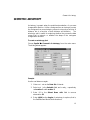
LOADING THE MODULE
The first step in using S+SPATIALSTATS 1.5 is to load the module.
Loading the module will make the spatial analysis functions available,
create the Spatial menu, and load the S+SPATIALSTATS 1.5 dialogs.
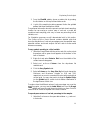
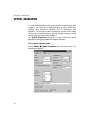
To load the module:
Choose File c Load Module from the main menu. The dialog
below appears:
To load the S+SPATIALSTATS 1.5 module, select spatial as the
Module and press OK.
A new menu selection, Spatial, will appear on the main S-PLUS menu
bar. Select this menu item to access the dialogs to analyze your spatial
data.
6
The Spatial Menu
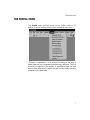
THE SPATIAL MENU
The Spatial menu provides access to the S+SPATIALSTATS 1.5
dialogs. To launch a dialog, simply select the desired menu item.
The menu is separated in three sections according to the type of
spatial data that the corresponding methodology applies to. The first
six items correspond to the analysis of geostatistical data, the next
three to data observed on a lattice, and the final two apply primarily
to spatial point pattern data.
7
Chapter 2 Getting Started
GETTING HELP
Help is available in a variety of ways:
8
•
Use the Help c S+SPATIALSTATS Help menu item to open
the S+SPATIALSTATS help file.
•
The Help button on a dialog will display help for that dialog.
•
The command line function help will provide help on a
specified function.
•
This supplement is also available online in a PDF file
viewable using Adobe Acrobat. Use the Help c Online
Manuals menu item to access it.
GEOSTATISTICAL DATA
3
Geostatistical data, also termed random field data, consist of
measurements taken at fixed locations. Variogram estimation and
kriging are commonly used with geostatistical data. These methods
were originally introduced as geostatistical methods for use in mining
applications. In recent years, these methods have been applied to
many disciplines including meteorology, forestry, agriculture,
cartography, climatology, and fisheries.
This section describes the following dialogs:
•
Variogram Cloud
•
Geometric Anisotropy
•
Empirical Variogram
•
Model Variogram
•
Ordinary Kriging
•
Universal Kriging
9
Chapter 3 Geostatistical Data
EXPLORATORY DATA ANALYSIS
In this section, we will give specific examples of EDA for geostatistical
data—data collected on a continuous spatial surface (see chapter 1 of
the S+SPATIALSTATS User’s Manual for a more precise definition).
The coal.ash data frame is used in an example of EDA for data
collected on an equally spaced grid of locations.
The coal.ash data will then be used to illustrate the use of the
S+SPATIALSTATS 1.5 dialogs to analyze geostatistical spatial data.
Example: The
Coal Ash Data
The coal.ash data come from the Pittsburgh coal seam on the
Robena Mine Property in Greene County, Pennsylvania (Cressie,
1993)1.
The data frame contains 208 coal ash core samples collected on a grid
given by x and y planar coordinates.
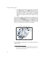
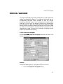
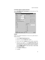
To plot the grid locations:
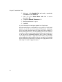
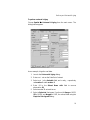
1. Open a view of the data on a Data Window. You can do this
by selecting Data c Select Data from the main menu and
then entering coal.ash as the Name of the existing data set
desired. The resulting dialog follows:
You could also use the command line directive:
> guiOpenView(Name=coal.ash, classname="data.frame")
2. Proceed by selecting the first 2 columns of the data frame in
the window.
1. Cressie, Noel A. C. (1993). Statistics for Spatial Data, Revised Edition.
John Wiley and Sons, New York.
10
Exploratory Data Analysis
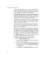
3. From the Plots2D palette, choose a scatter plot by pressing
the first button on the top left-hand side corner.
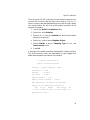
4. A plot of the sampling locations appears. Notice the gridded
pattern that these observations follow.
To superpose information about the percent coal ash at each sampling
location we can overlay a contour map of coal ash, or make the
symbols at each sampling point vary in some way according to that
variable, coal.
For illustration purposes, we will demonstrate both in this section.
The S+S PATIALSTATS User’s Manual contains detailed plots that
show the distribution of coal ash percentages over the sampled area,
potential outliers, and trend analysis. We will refer to those results
whenever necessary.
To vary symbols according to a third variable:
1. Select the Graph Sheet with the points, and click on the points
themselves until a green knob appears at the bottom of the
bulk of the data.
2. Right-click and select Data to Plot from the middle of the
context menu that appears.
3. Select coal as the z Column from the drop-down list
available and
4. Click the Vary Symbols tab.
5. Select z Column on the Vary Size By field, and change the
Minimum and Maximum Heights to 0.05 and 0.20,
respectively so as not to overwhelm the plot with symbols that
are too large. You may also want to change the Symbol Style
(on the Symbol tab) to a solid circle for better visualization of
the significance of their size.
To explore how the different values of coal percentage vary over the
sampling region, you may use the Label Point tool from the Graph
Tools palette and move through the points clicking on them. Point 50
seems to be an outlier as exposed in the User’s Manual.
To superimpose contours of coal ash percentage in the samples:
1. Select the 3 columns on the open data window: x, y, and coal
in that order.
11
Chapter 3 Geostatistical Data
2. Then select the graph region in the plot above and Shift-click
the Contours button on the Plots2D palette. Contour lines
varying with percentage of coal will be added to the plot of
the sampling locations. These contours are calculated
internally in S-PLUS using Akima’s fitting method (Akima,
1978)1. See the help file for the S-PLUS interp for more
detail.
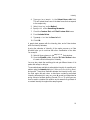
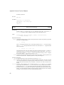
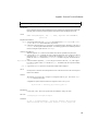
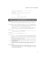
A few cosmetic changes can be made to the resulting plot. For
example, use the Gridding/Hist tab of the Contour Plot properties
dialog to clear the Extrapolation option and the Labels tab to add
labels to the contours (set Label Frequency to 1) and perhaps change
the font to make them more prominent. In the figure below, the
number of contours was also increased and a title inserted.
Coal Measurements and Sample Locations
22
17
y
12
7
2
2
6
10
14
x
The outlier, 17.6, is quite apparent and it is driving the shape of the
resulting contours.
1. Akima, H. (1978). A Method of Bivariate Interpolation and Smooth Surface Fitting for Irregularly Distributed Data Points. ACM Transactions on
Mathematical Software, 4, 148-164.
12
Variogram Cloud
VARIOGRAM CLOUD
The variogram cloud is a diagnostic tool that can be used to look for
potential outliers or trends, and to assess variability with increasing
distance. Anomalies and non-homogeneous areas can be detected by
looking at short distances that yield high dissimilarities.
To plot a variogram cloud:
Choose Spatial c Variogram Cloud from the main menu. The
dialog below appears:
Example:
Use the coal.ash data in the S+SPATIALSTATS data sets. From the
analysis in the User’s Manual, we know that these data exhibit a
strong East-West trend. The variogram values in the East-West
direction are likely influenced by the trend (the stationarity
13
Chapter 3 Geostatistical Data
assumption is violated in the presence of trend). We will restrict the
variogram cloud computations to points in a North-South direction by
manipulating the azimuth and its tolerance, as follows.
1. Launch the Variogram Cloud dialog.
2. Enter coal.ash as the Data Set to be analyzed.
3. Select coal as the Variable to be analyzed and select x, and
y, as Location 1 and Location2, respectively.
4. Change the Azimuth Tolerance from the omnidirectional
value of 90 degrees to a narrow .01.
5. Save the resulting object as coal.vgcloud.
6. Press OK.
A two-page Graph sheet appears containing a box plot and a scatter
plot of the variogram cloud. The variogram cloud shows a scatter of
high value points for the full range of distance values.
There is a method in S+SPATIALSTATS that can be used to identify
points in a variogram cloud; to invoke this method enter the
following command in the Commands Window while the Variogram
Cloud is the current active plot (this is required):
> identify(coal.vgcloud)
Identifying the high values in the variogram cloud shows that they all
are paired with observation 50, which was determined to be an
outlier indeed. We will remove observation 50 from further
variogram modeling.
The variogram cloud provides a diagnostic tool to look for potential
outliers or trends and to assess variability with increasing distance. It
provides the distribution of the variance between all pairs of points at
all possible distances and, as a consequence, it may yield extremely
dense point clouds that may be difficult to interpret. To reach a point
when we can model the variability in the data, a smoother version of
the variogram is available through the Empirical Variogram dialog.
14
Geometric Anisotropy
GEOMETRIC ANISOTROPY
Anisotropy is present when the spatial autocorrelation of a process
changes with direction. Unlike a variogram from an isotropic process,
the variogram from an anisotropic process is not purely a function of
distance, but is a function of both distance and direction.
The
anisotropy plot is useful for exploring whether the process the data
comes from is isotropic or whether the shape of the variogram
changes with direction.
To create an anisotropy plot:
Choose Spatial c Geometric Anisotropy from the main menu.
The dialog below appears:
Example:
Use the coal data once again:
1. Enter coal.ash as the Data Set of interest.
2. Select coal in the Variable field, and x and y, respectively
as Location 1 and Location 2.
3. Enter -50 in the Subset Rows with field to remove
observation 50.
4. Enter c(0,90) as the Angles of anisotropy to explore, that is,
the East-West and North-South directions.
15
Chapter 3 Geostatistical Data
5. Press OK.
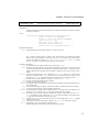
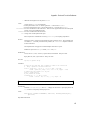
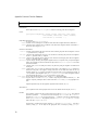
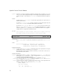
A multipanel plot appears in a Graph sheet, with several directional
variograms for all combinations of four ratio values for each of the 2
directions entered. The plot follows
2
0
2
90
2.2
2.0
1.8
1.6
1.4
1.2
1.0
5
10
15
20
0
10
20
1.75
0
30
40
1.75
90
2.2
2.0
1.8
1.6
1.4
1.2
gamma
1.0
5
10
15
20
0
10
20
1.5
0
30
40
1.5
90
2.2
2.0
1.8
1.6
1.4
1.2
1.0
5
10
15
20
5
10
15
1.25
0
20
25
30
1.25
90
2.2
2.0
1.8
1.6
1.4
1.2
1.0
5
10
15
20
5
10
15
20
25
distance
There are no apparent changes for differing ratio values (between
rows) but the variograms on the left do look different from those on
the right.
The Geometric Anisotropy dialog also provides an Options tab
where the user can specify parameters to control the estimation of the
variogram values for each combination of angle and ratio values. See
the dialog’s help file for detailed information or section 4.1.4 of the
S+SPATIALSTATS User’s Manual.
16
Empirical Variogram
EMPIRICAL VARIOGRAM
The empirical variogram provides a description of how the data are
related (correlated) with distance. The distances are binned and the
corresponding variogram values averaged for each bin thereby
producing a smoother version of the variogram which leads to easier
modeling. You can control the degree of smoothing by adjusting the
size of the “bins” or “lags”, the number of points in each bin, and the
distance of reliability (half the maximum distance over the field of data
by default) for the variogram. Several directional variograms can be
returned and as usual, a correction for Geometric Anisotropy can be
made to the data before processing.
To plot an empirical variogram:
Choose Spatial c Empirical Variogram from the main menu. The
dialog below appears:
Example:
Continue analyzing the coal.ash data in S+SPATIALSTATS.
1. Launch the Empirical Variogram dialog.
17
Chapter 3 Geostatistical Data
2. Select coal in the Variable field, and x and y, respectively
as Location 1 and Location 2.
3. Enter -50 in the Subset Rows with field to remove
observation 50.
4. Change the Azimuth Tolerance to .01.
5. Save the result as coal.vg.ns.
6. Press OK.
A plot of the empirical variogram appears in a Graph sheet.
Note that restricting our computation to only points in a North-South
direction is not the same as Correcting for Geometric Anisotropy.
When using the variogram values for those pairs that are related in a
North-South direction only, we are assessing one way the variancecovariance of the process changes without making any corrections to
it. We are trying to understand variability only in the N-S direction.
This makes some sense in applications that relate to physical data
where gradients are quite possible. Later on, we apply our knowledge
about this directional variation to the fitting of a kriging surface to the
data using Universal Kriging techniques.
18
Model Variogram
MODEL VARIOGRAM
In order to perform kriging, it is necessary to specify a theoretical
variogram function for the process. The Model Variogram dialog is
useful for examining the goodness-of-fit of various theoretical
variograms to the observed empirical variogram. Typically this dialog
will be used repeatedly to determine an appropriate variogram
function and parameter values.
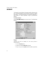
To fit a theoretical variogram:
Choose Spatial c Model Variogram from the main menu. The
dialog below appears:
Example:
Use the coal.ash data in S+SPATIALSTATS. Note that for the
purposes of this example we will fit a theoretical variogram to the
North-South empirical variogram we estimated above. In practice, we
want to first remove trend and explore the data further as is done in
the User’s Manual.
1. Launch the Model Variogram dialog.
2. Select the name of a fitted empirical variogram object from
the drop-down list in the Variogram Object field. Enter the
object saved after using the Empirical Variogram dialog,
coal.vg.ns.
19
Chapter 3 Geostatistical Data
3. Select a function to fit to the variogram, say a Spherical.
4. At this point you may check Fit Parameters and have the
variogram parameters fitted automatically using the
S+SPATIALSTATS function variogram.fit, or enter your
own. Check the Fit Parameters check box.
5. The parameters values are filled in automatically. Enter a
name in the Save As field to save the resulting variogram
model. Enter coal.vgmdl.
6. Press Apply.
You could also fit the variogram by trying different values of the
parameters and looking at the Objective Function. When doing this,
make sure that the Fit Parameters box is not checked.
1. The empirical variogram plot suggests that a Nugget of
around 0.7 and a Sill of around 1.1 are appropriate. Enter
these parameter values.
2. Now try various values of Range by entering them one at a
time and pressing Apply after each input. Look at the
resulting plot each time along with the objective value printed
on the plot to assess how well the specified theoretical
variogram matches the empirical variogram.
3. A Range of 6 gives a local minima in the objective value.
After we have selected this Range, we may wish to try other
values of Sill and Nugget to further reduce the objective
value.
4. Trying various values suggests that an empirical variance
function with range of 6.5, sill of 1.9, and nugget of 1.1
matches the empirical variogram pretty well. Enter these
values and press Apply.
5. Press OK or Cancel to dismiss the dialog.
Try fitting the variogram without removing observation 50 and see
how much influence this value has on the final variogram model. You
will need to fit an empirical variogram first and then proceed to the
Model Variogram dialog.
The results, saved in the object named as stated in the Save As field,
can be given to one of the kriging dialogs to fit a kriging surface to the
spatial process of interest.
20
Ordinary and Universal Kriging
ORDINARY AND UNIVERSAL KRIGING
Kriging is a linear interpolation method that allows predictions of
unknown values of a random field from observations at known
locations. Kriging incorporates a model of the covariance of the
random function when calculating predictions of the unknown values.
S+SPATIALSTATS provides two Kriging dialogs to support both
ordinary and universal kriging.
Ordinary kriging uses a random function model of spatial correlation to
calculate a weighted linear combination of available samples, for
prediction of a nearby unsampled location. Weights are chosen to
ensure that the average error for the model is zero and that the
modeled error variance is minimized.
Universal kriging is an adaptation of ordinary kriging that
accommodates trend. The trend is modeled as a polynomial function
of spatial location. Universal kriging can be used to both produce
local estimates in the presence of trend, and to estimate the
underlying trend itself. Universal kriging with a constant mean is
equivalent to ordinary kriging.
The Ordinary and Universal Kriging dialogs provide several
options for prediction. Block Kriging predictions (the average over a
rectangular area) are possible using the dialogs as well as Point
predictions either on a grid or at new sampling points.
Several different plots can be requested to help visualize both the
predictions and their standard errors.
21
Chapter 3 Geostatistical Data
To perform ordinary kriging:
Choose Spatial c Ordinary Kriging from the main menu. The
dialog below appears:
Example:
Let us krige the coal data.
1. Launch the Ordinary Kriging dialog.
2. Enter coal.ash as the Data Set of interest.
3. Select coal in the Variable field, and x and y, respectively
as Location 1 and Location 2.
4. Enter -50 in the Subset Rows with field to remove
observation 50.
5. Check the Use Values from a Variogram Fit box.
22
Ordinary and Universal Kriging
6. Select coal.vgmdl from the drop-down list in the
Variogram Fit field. This is the variogram.fit object that
we obtained using the Model Variogram dialog. The fields
for the Variogram parameters automatically fill.
7.
Save to an object named coal.ordKrige.
8. Move to the Plot tab. Specify Surface Plots for both the
predictions and their standard errors.
9. Press OK.
You see a summary of the fitted object, coal.ordKrige, in a Report
window, and the plot on different pages of a Graph sheet.
The exploratory plots of the data presented in the S+S PATIALSTATS
User’s Manual indicated the presence of a strong gradient in these
data. This gradient might be apparent if we plot the observations
against location.
To plot the coal observations against location:
1. Create a new data set by removing observation 50 from the
coal.ash data frame by entering these commands in the
Commands Window:
> coal.no50 <- coal.ash[-50,]
# Remove 50th row
2. Choose Data c Select Data from the main menu and open
the coal.no50 data frame.
3. Select columns x and coal.
4. From the Plots2D palette, choose a scatter plot with a loess
fit through it by pressing the corresponding button (a scatter
plot with an L on it).
5. Click on the graphsheet and choose Insert c Annotation c
Reference Line c Horizontal and add a horizontal dashed
line at the mean of the observations, that is set Position at
9.740725, to the plot of the observations against x.
6. Go back to the Data Window and select y and coal this time.
7.
Click on the graphsheet with the observations vs. x plot and
on the scatter plot with a loess fit on the Plots2D
palette. The plot of coal against y will be superimposed on
the other plot.
SHIFT-click
23
Chapter 3 Geostatistical Data
8. Separate the plots by clicking on the plot region (not on a data
point) and selecting Multipanel from the resulting menu.
9. Select By Plot as the Panel Type and set the Layout to be a 1
column by 2 rows plot arrangement.
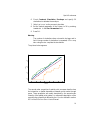
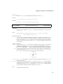
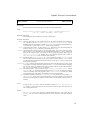
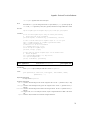
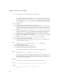
After inserting a title, you see the figure below:
Coal Ash % against Location
coal by y
13
coal
9
coal by x
13
9
0
5
10
15
20
25
The trend is apparent from the bottom plot. We will try to model this
trend as a second order polynomial in x as part of a Universal Kriging
fit in the following section.
24
Ordinary and Universal Kriging
To perform universal kriging:
Choose Spatial c Universal Kriging from the main menu. The
dialog below appears:
As an example, krige the coal data.
1. Launch the Universal Kriging dialog.
2. Enter coal.ash as the Data Set of interest.
3. Select coal in the Variable field, and x and y, respectively
as Location 1 and Location 2.
4. Enter -50 in the Subset Rows with field to remove
observation 50.
5. Select x and x^2 as trend terms.
6. Select a Spherical Variogram Function with Range of 6.570,
Sill of 0.109, and Nugget of 0.917, the values fitted using the
Empirical Variogram dialog.
25
Chapter 3 Geostatistical Data
7.
Save to an object named coal.krige.
8. Move to the Predict tab and check the boxes specifying that
the Predictions and Standard Errors should be saved. Enter
coal.kgpred in the Save In field.
9. Leave the Locations Type set to its default value of Grid.
The predicted values will be on a grid.
10. Move to the Plot tab. Specify Surface Plots for both the
predictions and their standard errors.
11. Press OK.
You see a summary of the fitted object, coal.krige, in a Report
window, and the plot on different pages of a Graph sheet, and a Data
window with the predictions.
A plot of both the predictions and their standard errors follows:
Kriging Predictions
Kriging Std. Errors
Compare this with Figure 4.25 of the S+SPATIALSTATS User’s
Manual. Other plots can be generated by having the prediction object
coal.kgpred open. Select 3 columns x, y, and fit, and try different
displays but pushing buttons on the Plots2D and Plots3D palettes.
You may want to rotate different graphs to look at the predictions
from several different angles.
26
Ordinary and Universal Kriging
Plotting the residuals from this fit produces a tighter fit about the 0
reference lines though there are still a few high values.
Residuals from Universal Kriging Fit
uniResid by y
3
uniResid
-1
uniResid by x
3
-1
0
Block Kriging
5
10
15
20
25
Block kriging is the general term used for the prediction of the average
value of a random field over a segment, surface, or volume. The term
Point kriging refers to prediction of the field at a point.
In S+SPATIALSTATS, block kriging is computed by the predict
method for objects of call "krige", predict.krige, and is
implemented on the Predict tab of both Kriging dialogs.
Block kriging is restricted to prediction of the average value over a
rectangular area. The integral over the block rectangular is
approximated by the average of the point predictions within the
block. You may control the number of points to be considered in the
average as well as the block size.
27
Chapter 3 Geostatistical Data
To perform block kriging on the coal data:
1. Choose Spatial c Universal Kriging from the main menu.
2. Use the rollback button at the bottom of the dialog to recover
the settings used in performing Universal Kriging on the coal
data.
3. Move to the Predict tab. The dialog below appears:
4. Enter coal.BKpred as the name of the object to save the
predictions in.
5. Check both Predictions and Standard Errors to be saved.
6. Choose Block as the Prediction Type.
7.
28
Specify a 1 x 1 block by entering 1 as the Block Length(X)
and the same as the Block Width (Y) (or leaving the default
values in).
Ordinary and Universal Kriging
8. Specify 5 as the number of points in the X direction to be
averaged for each block.
9. Specify also 5 points in the Y direction.
10. Click OK.
The predictions are calculated with the supplied prediction locations
in the center of the block. The block prediction will be the average of
point predictions at 25 locations within each block.
The predicted values are very similar to those obtain with the default
Point kriging when performing Universal Kriging. That is to be
expected.
The standard errors are much smaller for the block kriging since the
predictions are averages.
Kriging Std. Errors
29
Chapter 3 Geostatistical Data
30
LATTICE DATA
4
Lattice data are observations from a random process observed over a
countable collection of spatial regions, and supplemented by a
neighborhood structure. The observation locations can be regular
(equally spaced grid) or irregular, and data at a particular location
typically represent the entire region. The data observed at each site
may be continuous or discrete.
Before modeling the spatial component of lattice data in
S+SPATIALSTATS, we assume stationarity and multivariate normality
of the small-scale variation in the data, that is, of the error term. This
means that trend must be removed, and transformations may be
required to stabilize the variance and/or to approximate normality.
The primary tools available for examining lattice data are Spatial
Correlations and Spatial Regression. These dialogs require a data
set containing the observations at each location, and a spatial
neighbor object describing the spatial relationship between the
observations. The Spatial Neighbors dialog creates a spatial
neighbor object.
This section describes the following dialogs:
•
Spatial Neighbors
•
Spatial Correlations
•
Spatial Regression
31
Chapter 4 Lattice Data
EXPLORATORY ANALYSIS
The sample data frame sids contains spatial data collected on a
lattice. The collection points are counties in the state of North
Carolina, and the data are the rates of death from Sudden Infant
Death Syndrome (SIDS) for the years 1974-1978 (Cressie, 1993)1. The
components of the SIDS data frame are:
> names(sids)
[1] "id"
[5] "births"
[8] "sid.ft"
>
"easting"
"northing"
"nwbirths"
"group"
"nwbirths.ft"
"sid"
Data for the years 1979-1984 are also available in sids2. See the sids
help file for explanations of the individual variables.
To form a spatial lattice, you must have data locations and
neighborhood information. The locations for the SIDS data are stored
in easting and northing. Neighborhood information is typically
stored in a neighbor matrix, where two regions i and j are neighbors if
the ij-th element of the neighbor matrix is non-zero. In
S+SPATIALSTATS, neighbor information is stored in an object of class
“spatial.neighbor”, a sparse matrix representation of the neighbor
matrix. The S-PLUS object sids.neighbor already contains the
neighbor information for the SIDS data.
To summarize a spatial neighbor:
We can summarize the neighborhood information calling the
summary method for a spatial neighbor as follows:
> summary(sids.neighbor)
Matrix was NOT defined as symmetric
Number of Regions: 100
Average Number of Connections: 4.020408
Average Weight: 0.1306507
Least Number of Connections: 1 for Regions with Indices:
[1] 10 16 67
Maximum Number of Connections: 8 for Regions with Indices:
1. Cressie, Noel A. C. (1993). Statistics for Spatial Data, Revised Edition.
John Wiley and Sons, New York.
32
Exploratory Analysis
[1] 21
Missing Row Indices:
[1] 28 48
Missing Column Indices:
[1] 28 48
Indices of Regions with No Connections (islands):
[1] 28 48
>
The resulting summary describes the neighborhood as being defined
for 100 regions with varying neighbor weights. Each county has about
4 neighbors on the average with one county having 8 neighbors and 2
having none. The latter are known as “islands” in S+SPATIALSTATS.
We can use the row names of the data frame to determine which
neighbors are special.
> row.names(sids)[21]
[1] "Chowan"
> row.names(sids)[c(28,48)]
[1] "Dare" "Hyde"
>
Chowan has the most neighbors while Dare and Hyde counties are
isolated.
To plot a spatial neighbor object:
A neighbor object can be plotted from the Command line in version
1.5 of S+SPATIALSTATS by issuing a command such as
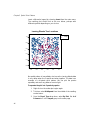
> plot(sids.neighbor, xc=sids$easting, yc=sids$northing,
+ scaled=T)
33
Chapter 4 Lattice Data
y
-200
-100
0
100
200
300
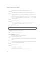
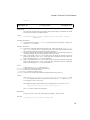
The following figure is produced:
100
200
300
400
x
We see, roughly, the shape of the state of North Carolina, as the
county seats are joined by line segments to indicate their neighbor
relationship.
34
Spatial Neighbors
SPATIAL NEIGHBORS
Lattice modeling is the spatial analogue to time series modeling. A
time series is modeled by predicting the outcome for each time based
on its dependence on the preceding observation or set of
observations. A spatial process is modeled by predicting the outcome
for each region based partially on its dependence on nearby or
neighboring regions. Choosing a neighborhood structure is the first
step in the analysis of lattice data. The result determines the
covariance structure used for the spatial component of a more general
linear regression model.
Neighbors may be defined as regions which border each other, or as
regions within a certain distance of each other. The neighbor
relationship is not necessarily symmetric. For example, the
underlying process may flow in only one direction, or a region that is
very large might exhibit influence on, but not be influenced by, a
smaller region. Since the neighborhood structure is the basic structure
for the covariance model for lattice data, the careful definition of
spatial neighbors is a crucial analysis step.
The Spatial Neighbors dialog provides a variety of ways to create a
spatial neighbor object.
35
Chapter 4 Lattice Data
To create a spatial neighbor object:
Choose Spatial c Spatial Neighbors from the main menu. The
dialog below appears:
Example:
Model the spatial neighborhood structure for the sids dataset in
S+SPATIALSTATS.
1. Launch Spatial Neighbors dialog.
2. Select Nearest Nhbrs as the source of neighborhood
information. This implies that the neighbors will be defined
by distances between point locations and so the location
variables will need to be provided.
3. Enter sids as the Data Set of interest.
4. Select easting and northing as Variables 1 and 2
respectively.
5. Specify Max Dist of 30, keeping Euclidean as the metric and
1 as the number of neighbors to consider.
6. Enter sids.nhbr30 in the Save In field.
36
Spatial Neighbors
7.
Press OK.
A Data Window opens containing the spatial neighbor object. We can
use this object to compute spatial correlations and perform spatial
regression.
Several sources are considered when using the Spatial Neighbors
dialog depending on how the neighborhood information is stored in
S-PLUS or on an ascii file to be read in. These are:
•
Nearest Nhbrs, to be used when you have point locations.
•
Row and Col ID, to enter data that is already paired up by
neighbors with row and column identifiers for each neighbor
pair.
•
Weight Matrix, if the square matrix containing the neighbor
weights is available for input.
•
Create Grid, to generate regular lattices.
•
Read File, to browse an ASCII file of varying record length
and a set of neighbors per row.
Click the Help button on the dialog for more specifics on each of
these options and the corresponding S+SPATIALSTATS function.
After using this dialog for your data, make sure that the results are
saved and then explore their structure with both the summary and
plot
methods illustrated above for objects of class
“spatial.neighbor”.
37
Chapter 4 Lattice Data
SPATIAL CORRELATIONS
If a process is spatially autocorrelated, there may be a need for spatial
modeling. A test for spatial autocorrelation can be performed as an
exploratory technique to decide whether spatial modeling should be
used. The null hypothesis is of no correlation, and the alternative
hypothesis is specifically defined by a weighted neighbor matrix. The
result is therefore sensitive to the choice of neighbors and weights, so
it may be desirable to run the autocorrelation under several different
scenarios. The calculation of spatial autocorrelation assumes constant
mean and variance. If the process contains trend or non-constant
variance, the results should be used with caution.
The Spatial Correlations dialog computes spatial autocorrelation
and related estimates of variation.
To compute spatial correlations:
Choose Spatial c Spatial Correlations from the main menu. The
dialog below appears:
Example:
Calculate Spatial Correlations for the sids data. If you haven’t
already used the data to create the spatial neighbor object
sids.nhbr30, follow the steps in the previous section before
proceeding.
38
Spatial Correlations
The occurrence of SIDS is not likely to have constant variance, since
counties with low birth rates will have more variance. The sid.ft
column contains rates standardized using the Freeman-Tukey square
root transformation. We will look at the spatial correlation of the
transformed variable.
1. Launch the Spatial Correlations dialog.
2. Select sids as the Data Set.
3. Select sids.ft from the Variables list. Notice that multiple
selections are allowed.
4. Select sids.nhbr30 as the Neighbor Object.
5. Specify Statistic of moran, Sampling Type of free, and
Num Permute of 100.
6. Press OK.
A summary of the spatial correlation is displayed in a Report window.
The small Normal p-value and permutation p-value suggest that
spatial autocorrelation is present for this variable.
*** Spatial Correlations **
Spatial Correlation Estimat
Statistic = "moran" Sampling = "free
Correlation =
Variance
=
Std. Error =
0.259
0.00478
0.0691
Normal statistic = 3.89
Normal p-value (2-sided) =
Null Hypothesis:
9.927e-
No spatial autocorrelati
Summary of the permutation-correlations
Min. 1st Qu.
Median
Mean 3rd Qu.
Ma
-0.1432 -0.08002 -0.01972 -0.01936 0.03252 0.15
permutation p-value =
39
Chapter 4 Lattice Data
SPATIAL REGRESSION
To model spatial lattices, we look at two levels of variation—large-scale
change in the mean due to spatial location or other explanatory
variables, and small-scale variation due to interactions with
neighbors. The change in mean is modeled as a linear model, taking
into account an autoregressive or moving average covariance model
reflecting the interactions with neighbors.
The Spatial Regression dialog fits a linear model with spatial
dependence using generalized least squares regression.
To fit a spatial regression model:
Choose Spatial c Spatial Regression from the main menu. The
dialog below appears:
40
Spatial Regression
Example:
Fit a Spatial Regression model to the sids data frame. See the
S+SPATIALSTATS User’s Manual for a detailed explanation on the
choice of regression variables and Covariance Model. This example is
equivalent to the example run on page 131 of the Manual.
1. Launch the Spatial Regression dialog.
2. Enter sids as the Data Set to be modeled.
3. Select the sid.ft and nwbirths.ft columns as Dependent
and Independent variables, respectively.
4. Enter -4 in the Subset Rows with field to remove
observation 4 as it was identified as an outlier in section 3.3 of
the User’s Manual.
5. Set the Cov Type to CAR.
6. Enter sids.neighbor as the Neighbor Object.
7.
To enter spatial weights, consult the help file for the
S+SPATIALSTATS function slm and enter the argument
weights=1/sids$births in the Parameters text box.
8. Enter sids.slm1 in the Save As field.
9. Press OK.
A summary of the spatial regression is displayed in a Report window.
It includes the actual call to the S+SPATIALSTATS function slm, the
coefficients of the regression, their variance-covariance matrix, and
other parameters of the spatial relationships and covariance matrix
structure. In particular, the coefficients for this model indicate a
highly significant effect of non-white births on rates of SIDS in North
Carolina.
Coefficients
Value Std. Error t value Pr(>|t
(Intercept) 1.6456 0.2385
6.8990 0.00
nwbirths.ft 0.0345 0.0066
5.2068 0.00
41
Chapter 4 Lattice Data
Diagnostic plots on the residuals should follow this analysis to assess
the adequacy of the model fitted. You can save the residuals by
indicating so in the Results tab of the Spatial Regression dialog.
Alternatively, you may extract them from the fitted model using the
residuals method as follows:
> sids.slm1.resid <- residuals(sids.slm1)
> summary(sids.slm1.resid)
Min. 1st Qu. Median Mean 3rd Qu. Max.
-106 -18.79
7.01 3.61
26.27 77.8
> qqnorm(sids.slm1.resid)
For example, the sequence of commands above would yield a
quantile-quantile normal plot of the residuals to assess the normality
assumption.
42
SPATIAL POINT PATTERNS
5
A mapped spatial point pattern is a collection of points located within
a bounded region of space. The points can denote locations of
naturally occurring phenomena such as earthquakes or plants, or
social events such as the locations of small towns or the occurrences
of a particular disease.
The data locations or points might be randomly located, tending to
cluster in groups, or follow a regular and predictable pattern. A
typical data analysis of a point pattern focuses on the question of
whether the point locations are completely spatially random (CSR) or
whether we should make an attempt to model an apparent lack of
spatial randomness.
Formal checks for CSR and modeling techniques for spatial point
patterns are described in chapter 6 of the S+SPATIALSTATS User’s
Manual. In this section, we describe ways to use the GUI of S-PLUS
and S+SPATIALSTATS to visualize spatial point patterns and to assess
the hypothesis of CSR.
A data set containing the mapped locations of maple and hickory
trees in a 19.6 acre square plot in Lansing Woods, Clinton County,
Michigan, will be used for the examples in this section (Diggle,
1983)1. The data have been scaled so that they reside on the unit
square, although this is not necessary for their analysis. See the User’s
Manual for a more complete description of the data set.
This section describes the following dialogs:
•
Spatial Randomness
•
Intensity
1. Diggle, Peter J. (1983). Statistical Analysis of Spatial Point Patterns. Academic Press Inc., New York.
43
Chapter 5 Spatial Point Patterns
EXPLORATORY ANALYSIS
The exploratory analysis of a spatial point pattern begins with a map
of the observations.
To view a spatial point pattern:
1. First open a view of the data on a Data Window. You can do
this by selecting Data c Select Data from the main menu
and then entering lansing as the Name of the existing data
set desired. The resulting dialog follows:
You could also use the command line directive:
> guiOpenView(Name=lansing, classname="data.frame")
2. Proceed by selecting all 3 columns of the data frame in the
window, starting with the first column, column x.
3. From the Plots2D palette, choose a scatter plot by pressing
the first button on the top left-hand side corner. A scatter plot
of the tree locations appears. In this scatter plot the points will
be plotted with a different symbol for each species.
You may change the symbol color and shape independently for each
species to suit your taste and help you differentiate the 2 species
better.
4. Position the cursor on a data point and right-click.
5. Select Symbol from the middle of the resulting context menu.
6. Change the symbol’s Style and Color as preferred, pressing
Apply to assess each change.
7.
Press OK, when satisfied.
8. Repeat steps 4-7 for the other symbol.
44
Exploratory Analysis
9. Chose Insert c Legend from the main menu and insert a
legend. Move the legend by dragging it and position as
desired on or outside the plot.
10. Chose Insert c Titles c Main from the main menu and
insert a title on top of the plot.
When plotting spatial data such as these, it is preferable to have both
axis scaled the same way for geometric accuracy, that is, a scale that
conforms to the actual observation locations.
To scale the axis:
1. Right-click on the plot region of the scatter plot (not on a data
point).
2. Select Position/Size from the middle of the resulting context
menu.
3. Change the Aspect Ratio from Auto to 1 (or set to
Proportional Units).
4. Click OK.
45
Chapter 5 Spatial Point Patterns
Insert a title and a legend by choosing Insert from the main menu.
The resulting plot would look as the one below, perhaps with
different symbols depending on your choice:
Lansing Woods Tree Locations
hickory
maple
1.0
0.8
y
0.6
0.4
0.2
0.0
0.0
0.2
0.4
0.6
0.8
1.0
x
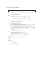
No spatial pattern is immediately obvious as the Lansing Woods data
is very dense when the 2 species are taken together. The data is an
example of a bivariate point pattern. We can plot the species
separately and see if any patterns come to light.
To separate the plot into 2 panels by species:
1. Right-click on the scatter plot region again.
2. This time, select Multipanel from the middle of the resulting
context menu.
3. From the Panel Type drop-down, select By Plot. Set # of
Columns to 2 in the Layout group on the same page.
46
Exploratory Analysis
4. Click OK.
The figure below appears. Reposition the legend to uncover the axes..
L a n s in g W o o d s T re e L o c a tio n s
h ic k o ry
m a p le
0 .2
h ic k o ry
0 .5
0 .8
m a p le
.8
.5
.2
0 .2
0 .5
0 .8
x
These plots show that there may be interaction between the two tree
species. It may be that the presence of one species inhibits the
presence of the other.
47
Chapter 5 Spatial Point Patterns
SPATIAL RANDOMNESS
Typical assumptions of interest for point pattern data are:
1. The intensity of the point pattern does not vary over the
boundary region.
2. There are no interactions among the points—points neither
inhibit nor encourage each other.
A spatial point pattern with these properties is said to be Completely
Spatially Random. See Chapter 6 of the S+SPATIALSTATS user’s
Manual for a more rigorous definition and further examples.
The Fhat and Ghat statistics are useful for assessing the first
assumption (constant intensity). The Khat and Lhat statistics are
useful for assessing the second assumption (second-order intensity
which does not depend on absolute location).
The Spatial Randomness dialog provides plots and saved values for
Fhat, Ghat, Khat, and Lhat.
48
Spatial Randomness
To calculate measures of spatial randomness:
Choose Spatial c Spatial Randomness from the main menu. The
dialog below appears:
Example:
Explore the Spatial Randomness of the lansing data frame in
S+SPATIALSTATS:
1. Launch Spatial Randomness dialog.
2. Enter lansing as the Data Set of interest.
3. Select x and y as the Location 1 and 2 variables, respectively.
4. Type species==”maple” in the Subset Rows with field.
This will subset those rows of the data frame that correspond
to the maples only. (Note that another approach would be to
choose Data c Subset from the main menu, to create a data
set of just the maples.)
5. Check Fhat and Ghat plots.
6. Press OK.
49
Chapter 5 Spatial Point Patterns
A Graph sheet opens displaying the Fhat and Ghat plots for the
maples. These are plots of the Empirical Distribution Function (EDF)
of the origin-to-point (Fhat) and the point-to-point (Ghat) nearest
neighbor distances for the maples in the Lansing Woods.
Values of Ghat are computed for every neighbor distance in the point
process by default. The grid of origins in the Fhat calculation is
determined by the square root of the total number of points in the
given point process. For more specifics on the calculations, consult
the individual S+SPATIALSTATS help files for Fhat and Ghat.
Visual judgement of Ghat is based on the fact that if there is clustering
in the data, we would expect to see an excess of short distance
neighbors, while if there is regularity in the data, then there would be
an excess of long distance neighbors.
The interpretation of the Fhat plot is opposite that of the Ghat plot.
An excess of high distance values is interpreted as clustering. As
before, we could compare this statistic to simulations from a CSR
process for a visual interpretation.
When edge effects need to be considered, we can assess the
hypothesis of CSR using Monte Carlo techniques. For example, we
can simulate the EDF of nearest neighbor distances from several
realizations of a CSR process on A, the region containing the original
point pattern. The average of the simulations provides a reference
line, and the maximum and minimum provide a simulation envelope.
The Spatial Randomness dialog provides the ability to draw
simulation envelopes for both the Khat and Lhat statistics.
To compute a simulation envelope for an estimate of Lhat:
1. Launch Spatial Randomness dialog.
2. Enter lansing as the Data Set of interest (or press the Roll
Back button and skip to step 5).
3. Select x and y as the Location 1 and 2 variables, respectively.
4. Type species=="maple" in the Subset Rows with field.
This will subset those rows of the data frame that correspond
to the maples only.
5. Check Lhat plot. The Khat/Lhat Options group is enabled.
50
Spatial Randomness
6. Check Construct Simulation Envelope and specify 50
simulations to estimate the envelope.
7.
Select "poisson" as the process to simulate.
8. Set the lambda parameter of the Poisson to 10 by entering
lambda=10 in the Sim. Parameters field.
9. Press OK.
Warning:
The number of simulations does not need to be large, and in
fact if a large number of simulations is requested, S-PLUS may
take a long time to complete the simulations.
The picture below appears:
Lhat
0.6
0.4
0.2
0.0
0.0
0.1
0.2
0.3
0.4
0.5
0.6
0.7
Distance
The second-order properties of spatial point processes describe how
the interaction or spatial dependence between points varies through
space. These properties are usually described by the second-order
intensity of the spatial point pattern. An alternative description of the
second order properties is defined by the K-function defined in section
6.3.2 of the S+SPATIALSTATS User’s Manual.
51
Chapter 5 Spatial Point Patterns
INTENSITY
The intensity of a point pattern is the mean number of points per unit
area. Intensity plots display a smooth estimate of intensity for a spatial
point pattern. The intensity estimate may be saved and displayed in a
Data window for further exploration using the point-and-click
graphics.
To calculate intensity:
Choose Spatial c Intensity from the main menu. The dialog below
appears:
Example:
Calculate and plot the intensity for the lansing data in
S+SPATIALSTATS
1. Launch Intensity dialog.
2. Enter lansing as the Data Set of interest.
3. Select x and y as the Location 1 and 2 variables, respectively.
52
Intensity
4. Type species=="maple" in the Subset Rows with field.
This will subset those rows of the data frame that correspond
to the maples only.
5. Select "binning" as the Method.
6. Specify 0.25 as the Smoothing Parameter.
7.
Check the Contour Plot, and Filled Contour Plot boxes.
8. Check Include Points.
9. Type maple.int into the Save In field.
10. Click OK.
A graph sheet appears with the intensity plots, and a Data window
with the intensity estimates.
Having the estimates of intensity of the maple process on a Data
Window helps you to continue with other visualization of the data.
For example:
11. Select all three columns in the maple.int Data window.
12. Open the Plots3D palette. Press the 32 Color Surface button
to create a filled surface plot of intensity.
You may also rotate the resulting plot and get different views of its
peaks and valleys in doing so.
Three methods are available to estimate the intensity of a spatial point
pattern using the Intensity dialog in S+SPATIALSTATS: binning, kernel,
and gauss2d. These three methods estimate the intensity locally over
the total region A, and return a data frame containing smoothed
intensity estimates which may vary over A, as well as interpolated x
and y values to facilitate plotting. Several S-PLUS 3D plot types can
then be used to visualize this variation and to assess the hypothesis of
a constant intensity throughout the sampling area.
53
Chapter 5 Spatial Point Patterns
The binning method uses a two-dimensional histogram to form
rectangular bins. The counts in these bins are smoothed using a loess
smoothing algorithm. Using the binning method for the maple data as
explained in the sequence above yielded the following plot:
0 .2
0.
0.8
1
0.
0 .4
2
0 .4
0.6
0.2
0.2
y
0.0
0 .3
0.
1
0.4
0 .2
0.
0.2
4
0.
0.
3
0.
3
4
0 .4
0 0.
0 . .1 2
0
0.0
0.1
0.3
0.5
x
0.7
0.9
All of the intensity estimation and other visualization techniques used
in this section show that the intensity of the maple trees in the Lansing
Woods appears to vary more than would be expected by random
fluctuations. This might be due to the deficit of maple trees in the
north corners of the plot, which might be explained by interaction
with hickory trees.
54
Appendix: Data and Function Reference
APPENDIX A: DATA AND
FUNCTION REFERENCE
A
The functions and data sets described in this appendix are included
with S+SPATIALSTATS. The information in this appendix is also found
in the online help. For more information on accessing the online help,
see Chapter 2, Getting Started.
55
Appendix: Data and Function Reference
56
Appendix: Data and Function Reference
anisotropy.plot
Explore Corrections For Geometric Anisotropy
anisotropy.plot
DESCRIPTION
Computes corrections for geometric anisotropy for two dimensional spatial data and plots variograms
based on the corrections.
USAGE
anisotropy.plot(formula=formula(data), data=sys.parent(),
subset, na.action, lag=<<see below>>,
nlag=20, tol.lag=lag/2, maxdist=<<see below>>,
angle=c(0, 45, 90, 135),
ratio=seq(1.25, 2, length = 4),
minpairs=6, method="classical",
smooth=T, plot.it=T, panel=panel.xyplot, ...)
REQUIRED ARGUMENTS
formula formula defining the response and the predictors. In general, its form is:
z ˜ x + y
The z variable is a numeric response. Variables x and y are the locations. All variables in the formula
must be vectors of equal length with no missing values (NAs). The formula may also contain expressions for the variables, for example, sqrt(count), log(age+1) or I(2*x). (The I() is required
since the * operator has a special meaning on the right side of a formula.)
OPTIONAL ARGUMENTS
data an optional data frame in which to find the objects mentioned in formula.
subset expression saying which subset of the rows of the data should be used in the fit. This can be a logical
na.action
lag
nlag
tol.lag
maxdist
angle
ratio
minpairs
method
smooth
panel
plot.it
...
vector (which is replicated to have length equal to the number of observations), or a numeric vector indicating which observation numbers are to be included, or a character vector of the row names to be included.
a function to filter missing data. This is applied to the model.frame after any subset argument has
been used. The default (with na.fail) is to create an error if any missing values are found. A possible alternative is na.omit, which deletes observations that contain one or more missing values.
a numeric value, the width of the lags. If missing, lag is set to maxdist / nlag.
an integer, the maximum number of lags to calculate.
a numeric value, the distance tolerance.
the maximum distance to include in the returned output. The default is half the maximum distance in
the transformed data.
a vector of direction angles (in degrees, clockwise from North) to consider as directions of anisotropy.
a vector of ratios of anisotropy. These should all be greater than 1.
the minimum number of pairs of points (minimum value for np) that must be used in calculating a variogram value. If np is less than minpairs, that value is dropped from the variogram.
a character string to select the method for estimating the variogram. The possible values are "classical" for Matheron’s (1963) estimate and "robust" for Cressie and Hawkins (1980) robust estimator. Only the first character of the string needs to be given.
a logical flag, if TRUE, a loess smooth line is drawn for each variogram panel. If panel is supplied
then this value is ignored.
a panel function to be used in plotting the variograms. If plot.it=FALSE, this value is ignored.
a logical flag, if TRUE, a plot of all the variogram is drawn.
additional arguments to be passed down to the panel function for plotting.
57
Appendix: Data and Function Reference
VALUE
distance
gamma
np
angle
ratio
a data frame with columns:
the average distance for pairs in the lag.
the variogram estimate.
the number of pairs in each lag.
a factor denoting the angle for the geometric anisotropy.
a factor with levels denoting the ratio for the geometric anisotropy.
SIDE EFFECTS
If plot.it=TRUE (the default) the variogram for each combination of angle and ratio is plotted.
The plot is drawn using xyplot.
DETAILS
For each combination of angle and ratio the locations are corrected for geometric anisotropy. The
correction consists of multipling each location pair (x[i],y[i]) by the symmetric 2 x 2 matrix A
where A[1,1]=cos(angle)ˆ2+ratio*sin(angle)ˆ2, A[1,2]=(1- ratio) * sin(angle) *
cos(angle) and A[2,2]=sin(angle)ˆ2+ratio*cos(angle)ˆ2. See Journel and Huijbregts
(1978, pp 179-181). The variogram is then estimated using these corrected locations.
REFERENCES
Cressie, N. and Hawkins, D. M. (1980). Robust estimation of the variogram. Mathematical Geology
12, 115-125.
Journel, A. G. and Huijbregts, Ch. J. (1978). Mining Geostatistics. Academic Press, New York.
Matheron, G. (1963). Principles of geostatistics. Economic Geology 58, 1246-1266.
SEE ALSO
loc, variogram, xyplot.
EXAMPLES
anisotropy.plot(log(tcatch+1) ˜ long + lat, data=scallops, lag=.075)
check.islands
Detect Isolated Spatial Regions
check.islands
DESCRIPTION
Given an object of class "spatial.neighbor" detects spatial units that have no neighbors (islands).
USAGE
check.islands(x, remap=F)
REQUIRED ARGUMENTS
x an object of class "spatial.neighbor".
OPTIONAL ARGUMENTS
remap logical flag: if there is an island, should we recode the indexing of the spatial contiguity matrix to eliminate the rows and columns with all zeroes? That is, should we renumber components row.id and
col.id of the spatial neighbor object?
VALUE
if remap=FALSE the list of existing islands is returned. Otherwise, an object of class "spatial.neighbor" with remapped row.id and col.id.
58
Appendix: Data and Function Reference
SIDE EFFECTS
the attribute "nregion" of the output may differ from that of x whenremap=T.
SEE ALSO
spatial.neighbor, spatial.subset, spatial.weights
EXAMPLES
sids.nhbr2 <- check.islands(sids.neighbor,remap=T)
find.neighbor
Find the Nearest Neighbors of a Point
find.neighbor
DESCRIPTION
Find the k nearest neighbors of a vector x in a matrix of data contained in an object of class
"quad.tree".
USAGE
find.neighbor(x, quadtree=quad.tree(x), k=1, metric="euclidean",
max.dist=NULL, drop.self=F)
REQUIRED ARGUMENTS
x a vector (or matrix) containing the multidimensional point(s) at which the nearest neighbors are de-
sired. The vector must have the same number of elements as the number of columns in the numeric
matrix used to construct quadtree. If a matrix is used, the matrix must have the same number of
columns as the numeric matrix used to construct quadtree, and nearest neighbors are found for each
row in the matrix.
OPTIONAL ARGUMENTS
quadtree an object of class "quad.tree" containing the sorted matrix of data for which a nearest neighbor
search is desired. Defaults to quad.tree(x) if x is a matrix but it is required when x is a vector.
k the number of nearest neighbors to be found. If the data x is the same data that was used to construct
the "quad.tree" object, then k = 1 results in each element having itself as its own nearest neighbor.
metric a character string giving the metric to be used when finding "nearest" neighbors. Partial matching is allowed. Possible values are: "euclidean", "city block", and "maximum absolute value" for
the l 2 , l 1 , and l ∞ norm, respectively. For two vectors x and y, these are defined as:
l 1 = Σ |x i − y i |,
i
l2 =
Σ(x − y )
√
i
i
2) ,
i
l ∞ = max |x i − y i |
i
max.dist if max.dist is given, argument k is ignored, and all of the neighbors within distance max.dist of
each row in x are found.
drop.self a logical value, if TRUE then rows with distances equal to 0 and index1 == index2 (self neighbors)
are dropped from the returned object. This definition retains coincident points as neighbors although
their distance apart is zero. If quadtree is not supplied, k=1, and drop.self=T, a warning is printed
(since this results in nothing being returned) and the value of k is set to 2.
VALUE
a matrix with three named columns:
59
Appendix: Data and Function Reference
index1 if x is a matrix, the row in x for this nearest neighbor. If x is not a matrix, the value 1.
index2 the row in the matrix from which the quad tree was formed for this nearest neighbor. If the quad tree
was formed from a matrix y, then x[index1[i],] and y[index2[i],] are neighbors.
distances the corresponding nearest neighbor distances.
DETAILS
An efficient recursive algorithm is used to find all nearest neighbors. First the quad tree is traversed to
find the leaf with medians nearest the point for which neighbors are desired. Then all observations in
the leaf are searched to find nearest neighbors. Finally, if necessary, adjoining leaves are searched for
nearest neighbors.
REFERENCES
Friedman, J., Bentley, J. L., and Finkel, R. A. (1977). An algorithm for finding best matches in logarithmic expected time. ACM Transactions on Mathematical Software 3, 209-226.
SEE ALSO
quad.tree.
EXAMPLES
x <- cbind(sids$easting, sids$northing)
sids.nhbr <- find.neighbor(x, max.dist = 30)
# Find the nearest neighbors for the Lansing hickories
hickory <- lansing[lansing[,3] == "hickory", 1:2]
hickory.nhbr1 <- find.neighbor(hickory, k=2, drop.self=T)
# Now find the closest maple for each hickory
maple <- lansing[lansing[,3] == "maple", 1:2]
hmn <- find.neighbor(hickory, quad.tree(maple))
# and plot the tree locations with lines joing the neighbors
par(pty=’s’)
plot(maple[,1], maple[,2], pch=16)
points(hickory[,1], hickory[,2], pch=1, col=2)
segments(hickory[hmn[,1],1], hickory[hmn[,1],2],
maple[hmn[,2],1], maple[hmn[,2],2])
Glasgow.neighbor
Neighbors for Glasgow Mortality Rate Data
Glasgow.neighbor
SUMMARY
An object of class "spatial.neighbor" containing the neighbor specification among the 87 community medicine areas in Glasgow, Scotland. The standardized mortality rate (SMR) values for this
data are contained in Glasgow.SMR.
DATA DESCRIPTION
Four hundred and fifty neighbor relationships are specified. The neighbor relationships are not symmetric. See spatial.neighbor.object for a description of the data within an object of class
"spatial.neighbor".
SOURCE
The data are presented and analyzed in Haining (1990).
60
Appendix: Data and Function Reference
REFERENCES
Haining, R. (1990). Spatial Data Analysis in the Social and Environmental Sciences. Cambridge University Press. Cambridge.
SEE ALSO
Glasgow.SMR.
Glasgow.SMR
Standardized Mortality Rates for Glasgow
Glasgow.SMR
SUMMARY
The Glasgow.SMR data frame contains standardized mortality rates for 87 community medicine areas
in Glasgow, Scotland for 1980-1982.
DATA DESCRIPTION
This data frame contains the following columns:
the standardized mortality rate (SMR) for all deaths.
the SMR for death by accidents.
the SMR for deaths due to cancer.
the SMR for deaths due to respiratory disease accidents.
the SMR for deaths due to ischaemic heart disease.
the SMR for deaths due to cerebrovascular disease.
the population (in 1000’s).
the x coordinate of the community medicine area (CMA) relative to an arbitrary origin, where the x-axis is parallel to the latitude.
Northing the y coordinate of the CMA relative to an arbitrary origin, where the y-axis is parallel to the longitude.
AllDeaths
Accidents
Cancer
Respiratory
Heart
Cerebrovascular
Population
Easting
DETAILS
The standardized mortality rate for a community medicine area is the observed deaths due to that cause
divided by the expected number of deaths given the age and sex combination in that area multiplied by
100.
SOURCE
The data are presented and analyzed in Haining (1990).
REFERENCES
Haining, R. (1990). Spatial Data Analysis in the Social and Environmental Sciences. Cambridge University Press. Cambridge.
SEE ALSO
Glasgow.neighbor.
61
Appendix: Data and Function Reference
Kenv
Compute Simulations of Khat
Kenv
DESCRIPTION
Computes Khat (Lhat) for simulations of point processes. Returns upper and lower bounds, as well
as the average of all simulated values.
USAGE
Kenv(object, nsims=100, maxdist=<<see below>>, ndist=100,
process="binomial", boundary=bbox(object), add=T, ...)
Lenv(object, nsims=100, maxdist=<<see below>>, ndist=100,
process="binomial", boundary=bbox(object), add=T, ...)
REQUIRED ARGUMENTS
object an object of class "spp" representing a spatial point pattern, or a data frame or matrix with first two
columns containing locations of a point pattern.
OPTIONAL ARGUMENTS
nsims integer. Number of desired simulations.
maxdist numeric value indicating the maximum distance at which Khat (or Lhat) should be estimated. De-
faults to half the length of a diagonal of the sample’s bounding box.
ndist desired number of default distances at which to compute Khat (or Lhat). Default is 100.
process a character string with one of five possible processes for the spatial arrangement of the resulting pattern. This must be one of "binomial", "poisson", "cluster", "Strauss", or "SSI". See the
help file for make.pattern for information on parameters for each process.
add logical flag: should the envelope be added to an already existing plot of Khat (or Lhat for Lenv)? Defaults to TRUE.
... other parameters as needed by the requested process.
VALUE
dist
lower
upper
average
invisibly returns a list with 4 numeric vectors each representing:
the distances at which all values were computed.
the minimum of all resulting Khat (or Lhat for Lenv) for the simulations.
the maximum of all resulting Khat (or Lhat for Lenv) for the simulations.
the average of all resulting Khat (or Lhat for Lenv) for the simulations.
SIDE EFFECTS
if add=TRUE an envelope is added to an existing plot of Khat.
SEE ALSO
Khat, Lhat, make.pattern.
EXAMPLES
Khat(bramble)
Kenv(bramble,nsims=50)
Lhat(lansing)
Lenv(lansing,nsims=50)
62
Appendix: Data and Function Reference
Khat
Ripley’s K Function for a Spatial Point Pattern Object
Khat
DESCRIPTION
Calculates K(t), Ripley’s K function for a spatial point pattern.
USAGE
Khat(object, maxdist=<<see below>>, ndist=100, boundary=bbox(object),
plot.it=T)
REQUIRED ARGUMENTS
object an object of class "spp" representing a spatial point pattern, or a data frame or matrix with first two
columns containing locations of a point pattern.
OPTIONAL ARGUMENTS
maxdist numeric value indicating the maximum distance at which Khat should be estimated. Defaults to half
the length of a diagonal of the sample’s bounding box.
ndist desired number of default distances at which to compute Khat. Default is 100. The distances for
which Khat will be estimated are calculated as seq(0,maxdist,ndist), both maxdist and ndist
will change if not reasonable for the given object.
boundary points defining the boundary polygon for the spatial point pattern. This version accepts only rectangles, for which boundary should be given as a list with named components "x" and "y" denoting the
corners of the rectangular region. For example, for the unit square the boundary could be given as
bbox(x=c(0,1),y=c(0,1)), the bounding box of two diagonally opposed points. Defaults to a
rectangle covering the range of points.
plot.it logical flag: should the resulting K-estimates be plotted? Default is TRUE.
VALUE
a list containing components :
values a two column matrix. The first column, named dist, contains the distances at which Khat was computed, and the second column, named Khat, contains the values of K(dist).
ndist number of distances returned. This could be smaller than its input value if the extent of the distances is
too large.
mindist minimum distance between any pair of points.
maxdev maximum deviation from K(t)=t. See DETAILS.
SIDE EFFECTS
if plot.it=TRUE, a plot of the value of K(t) against distance will be produced on the current graphics device.
DETAILS
Khat computes Ripley’s (1976) estimate of K(t) for a spatial point pattern:
K (t) = λ −1 E[number of events ≤ distance t of an arbitrary event].
where λ is the intensity of the spatial point pattern.
The theoretical K-function for a Poisson (completely spatially random) process is K (t) = π t 2 , so
L(t) = √
K (t)/π is equal to t, the distances. The default plots K(t) versus t. See function Lhat for
estimation of L(t).
REFERENCES
Ripley, Brian D. (1976). The second-order analysis of stationary point processes. Journal of Applied
63
Appendix: Data and Function Reference
Probability, 13,255-266.
SEE ALSO
Kenv, Lhat.
EXAMPLES
lansing.spp <- as.spp(lansing)
lansing.khat <- Khat(lansing.spp)
Khat(wheat)
abline(0,1)
krige
Ordinary and Universal Kriging
krige
DESCRIPTION
Performs ordinary or universal kriging for two dimensional spatial data. The function predict.krige can then be called to compute interpolation surfaces and prediction errors.
USAGE
krige(formula, data=sys.parent(), subset, na.action=na.fail,
covfun, nc=10000, ...)
REQUIRED ARGUMENTS
formula a formula describing the kriging variable and the spatial location variables and optionally a polynomial
trend surface. Its simplest form is:
z ˜ loc(x,y)
where z is the kriging variable and x and y are the spatial locations, that is, z[i] is observed at the location (x[i],y[i]). The right hand side must contain a call to the function loc. A polynomial trend
surface is of the form:
z ˜ loc(x,y) + x + y + xˆ2 + yˆ2
The polynomial must be in the same variables as the first two arguments used in the loc function. A
constant term is always fit. All terms on the right hand side must be entered with a + sign. The loc
call can include arguments angle and ratio to correct for geometric anisotropy; see the loc help file.
Note that an evaluated loc object cannot be used in formula.
covfun a function that returns the distanced based covariance between two points. The first argument to the
function must be the distance. Additional parameters will be passed through the ....
OPTIONAL ARGUMENTS
data an optional data frame in which to find the objects mentioned in formula.
subset expression saying which subset of the rows of the data should be used in the fit. This can be a logical
vector (which is replicated to have length equal to the number of observations), or a numeric vector indicating which observation numbers are to be included, or a character vector of the row names to be included.
na.action a function to filter missing data. This is applied to the data in formula after any subset argument
has been used. The default (with na.fail) is to create an error if any missing values are found. A
possible alternative is na.omit, which deletes observations that contain one or more missing values.
nc the number of points to use internally by the algorithm in approximating the distance-based covariance
function. Note: this argument has nothing to do with the number of observed points used in computing
the kriging. All observed points are used in computing kriging predictions.
64
Appendix: Data and Function Reference
... additional named arguments can be passed to covfun.
VALUE
an object of class "krige" with components:
x the first spatial location vector i.e. the first argument in loc function call in formula.
y the second spatial location vector i.e. the second argument in loc function call in formula.
coefficients the vector of coefficients for the trend surface. These are for the polynomial based on the scaled spatial
location vectors (see the DETAILS section).
residuals the vector of residuals from the trend surface.
call an image of the call that produced the object.
Other components are included that are used by predict.krige for computing interpolations.
DETAILS
The kriging system is solved using generalized least squares (see Ripley, 1981). The polynomial terms
are scaled to (-1, 1) internally to avoid numeric problems; the coefficients component returned is
for these scaled terms.
This implementation of kriging does not handle multiple observations at a point.
Methods for objects of class "krige" include predict and print.
REFERENCES
Cressie, Noel A. C. (1993). Statistics for Spatial Data, Revised Edition. Wiley, New York.
Ripley, Brian D. (1981). Spatial Statistics. Wiley, New York
SEE ALSO
exp.cov, loc, predict.krige.
EXAMPLES
# krige the Coal Ash data with a quadratic trend in the x direction
#
using a spherical covariance function:
kcoal <- krige(coal ˜ loc(x, y) + x + xˆ2, data = coal.ash,
covfun = spher.cov, range = 4.31, sill = 0.14, nugget = 0.89)
# predictions over default 30 x 30 grid
pcoal <- predict(kcoal)
# plot prediction surface
wireframe(fit ˜ x * y, data = pcoal,
screen = list(z = 300, x = -60, y = 0), drape = T)
Lhat
Ripley’s K Function for a Spatial Point Pattern Object
Lhat
DESCRIPTION
Calculates L(t)=sqrt(K(t)/pi), where K(t) is Ripley’s K function for a spatial point pattern and
L(t) is linear for a completely random point process.
USAGE
Lhat(object, maxdist=<<see below>>, ndist=100, boundary=bbox(object),
plot.it=T)
REQUIRED ARGUMENTS
65
Appendix: Data and Function Reference
object an object of class "spp" representing a spatial point pattern, or a data frame or matrix with first two
columns containing locations of a point pattern.
OPTIONAL ARGUMENTS
maxdist numeric value indicating the maximum distance at which Lhat should be estimated. Defaults to half
the length of a diagonal of the sample’s bounding box.
ndist desired number of default distances at which to compute Lhat. Default is 100. The distances for
which Lhat will be estimated are calculated as seq(0,maxdist,ndist), both maxdist and ndist
will change if not reasonable for the given object.
boundary points defining the boundary polygon for the spatial point pattern. This version accepts only rectangles, for which boundary should be given as a list with named components "x" and "y" denoting the
corners of the rectangular region. For example, for the unit square the boundary could be given as
bbox(x=c(0,1),y=c(0,1)), the bounding box of two diagonally opposed points. Defaults to a
rectangle covering the range of points.
plot.it logical flag: should the resulting K-estimates be plotted? Default is TRUE.
VALUE
a list containing components :
values a two column matrix. The first column, called dist, contains the distances at which Lhat was computed, and the second column, called Lhat, contains the values of L(dist).
ndist number of distances returned. This could be smaller than its input value if the extent of the distances is
too large.
mindist minimum distance between any pair of points.
maxdev maximum deviation from L(t)=t. See DETAILS.
SIDE EFFECTS
if plot.it=TRUE, a plot of the value of L(t) against distance will be produced on the current graphics device.
DETAILS
Khat computes Ripley’s (1976) estimate of K(t) for a spatial point pattern:
K (t) = λ −1 E[number of events ≤ distance t of an arbitrary event].
where λ is the intensity of the spatial point pattern.
The theoretical K-function for a Poisson (completely spatially random) process is K (t) = π t 2 , so
L(t) = √
K (t)/π is equal to t, the distances. The default plots L(t) versus t which should approximate
a straight line for a homogeneous process with no spatial dependence. See function Khat for estimation of K(t).
REFERENCES
Ripley, Brian D. (1976). The second-order analysis of stationary point processes. Journal of Applied
Probability 13,255-266.
SEE ALSO
Lenv, Khat.
EXAMPLES
lansing.spp <- as.spp(lansing)
lansing.khat <- Lhat(lansing.spp)
Lhat(wheat)
abline(0,1)
66
Appendix: Data and Function Reference
make.pattern
Generate a Spatial Point Process
make.pattern
DESCRIPTION
Generates points in two-dimensional space given their desired spatial distribution.
USAGE
make.pattern(n, process="binomial", object, boundary=bbox(x=c(0,1),
y=c(0,1)), lambda, maxlambda, radius, cpar)
REQUIRED ARGUMENTS
n integer denoting the desired number of points in the resulting object.
OPTIONAL ARGUMENTS
process a character string with one of five possible processes for the spatial arrangement of the resulting pattern. This must be one of "binomial", "poisson", "cluster", "Strauss", or "SSI". See the
DETAILS section for each definition. Defaults to "binomial" for a completely spatially random process conditioned to n points within boundary. Partial matching is allowed.
object a spatial point pattern object. An object of class "spp". When this is given, the resulting pattern has
the same n and its boundary is that same as the bounding box of object.
boundary points defining the boundary polygon for the spatial point pattern. This version accepts only rectangles, for which boundary should be given as a list with named components "x" and "y" denoting the
corners of the rectangular region. For example, for the unit square the boundary could be given as
bbox(x=c(0,1),y=c(0,1)), the bounding box of two diagonally opposed points. Defaults to
bbox(object) if object is given or to the unit square otherwise.
lambda the intensity when process="poisson". If lambda is a numerical value then make.pattern simulates a two dimensional homogeneous Poisson process with that constant intensity. lambda can also
be a function with two arguments that defines the intensity over the region. n, if given, will be ignored
if this argument is provided.
maxlambda if lambda is a function then this should be the maximum value of the function over the region. If this
is not supplied, a nonlinear optimization will be run (using nlminb) to find the maximum. Supplying
this value will speed up the simulation and avoid any possible problems with the nonlinear optimization. maxlambda is used only if lambda is a function.
radius the inhibition distance. This is needed for process "Strauss", "SSI" and "cluster". Options
"Strauss" and "SSI" will NOT generate points closer than radius. For this reason, this parameter
needs to be reasonably small. The exception is when process="cluster" in which case it should
contain the desired size of the clusters. See DETAILS section for more information.
cpar the inhibition parameter needed when process="Strauss". This parameter is also required if process="cluster". In that case, it represents the intensity of the "parent" Poisson process which will
determine the random placement of clusters and their number. See the DETAILS section for more information.
VALUE
an object of class "spp" whose n points are distributed according to process. If process="poisson" results on a process with zero points, the returned value will be a classless matrix with zero rows
and a warning will be issued.
DETAILS
The "binomial" process option generates a spatially random pattern of n points within the given
boundary. This is in essence a homogeneous Poisson process conditional on the given number of
points n.
67
Appendix: Data and Function Reference
The "poisson" process option generates a Poisson process with intensity lambda. This argument is
required for this option. If lambda is a function the Poisson process is generated by a rejection sampling algorithm (Diggle, 1983): a homogeneous Poisson process with intensity maxlambda is generated over the region and then points are retained with probability lambda(x, y)/maxlambda.
The "SSI" process generates a random pattern where no two points are within the inhibition distance
determined by its parameter radius. This process is equivalent to sequentially laying down discs of
radius radius which will not overlap.
The "Strauss" process accepts each randomly generated point with probability cparˆs where s is
the number of existing points within radius radius of the potential new point. The parameter cpar
must be in [0,1] for this process, where cpar=0 corresponds to complete inhibition at distances up to
radius.
The user should exercise caution when determining the value of radius, for if it is too big in relation
to the area defined by boundary, the algorithm will run out of possible area to place the subsequent
disc and the generation of the desired process may be impossible or very slow.
The option "cluster" generates a Poisson cluster process. This is defined by generating a "parent"
Poisson process with intensity cpar and a "daughter" process of clusters with radii determined by the
value of radius.
WARNING
If radius is too large, it may be impossible or nearly impossible to generate the number of requested
points. The call may "hang" in some extreme cases.
REFERENCES
Diggle, Peter J. (1983). Statistical Analysis of Spatial Point Patterns. Academic Press, London.
Ripley, Brian D. (1981). Spatial Statistics. John Wiley & Sons, New York.
Ripley, Brian D. (1976). The second-order analysis of stationary point processes. Journal of Applied
Probability 13,255-266.
SEE ALSO
runif, rnorm, rpois, rbinom.
EXAMPLES
# A completely random process in the unit square
rand <- make.pattern(100)
plot(make.pattern(100, process="Strauss", rad=0.1, c=0.5))
plot(make.pattern(500, proc="cluster", rad=20, c=10,
boundary=list(x=c(0,200), y=c(0,200))))
# A nonhomogeneous Poisson pattern with a linear trend in x
# over a 10 x 10 square
lxy <- function(x, y) 1.5*x
xy <- make.pattern(proc="poisson", boundary=bbox(x=c(0,10),
y=c(0,10)), lambda=lxy)
plot(xy)
68
Appendix: Data and Function Reference
model.variogram
Display a Variogram Object and Theoretical Model
model.variogram
DESCRIPTION
Plots an empirical variogram object and displays the fit of a theoretical variogram model on that plot.
Optionally allows interactive parameter updates to the theoretical model and displays the new fit.
USAGE
model.variogram(object, fun, ..., ask=T, objective.fun=<<see below>>,
plot.it=T)
REQUIRED ARGUMENTS
object an object that inherits from class "variogram" (this includes classes "covariogram" and "correlogram"). The azimuth column should have only one level.
fun a theoretical variogram function (or covariogram or correlogram function, depending on the class of
"object"). Its first argument should be distance. Its remaining arguments are considered parameters
that can be changed to update the fit of fun to object.
OPTIONAL ARGUMENTS
... additional arguments to fun that do not have default values must be specified here by full name.
ask a logical value, if TRUE, a command line menu is displayed allowing the user to change the values of
the parameters to fun. After changing a value the plot is updated. If FALSE, the data in object is
plotted, the value of fun evaluated at object$distance is added to the graph, and the function re-
turns.
objective.fun a function with three arguments, y, yf, and n that gives a measure of the fit of yf to y with weights n.
It is used as a measure of fit of fun to the data in object. The default is the sum of squared residuals,
sum((y-yf)ˆ2).
plot.it a logical value, if TRUE, a plot of the variogram and its fitted model is displayed.
VALUE
invisibly returns a named list of the final parameters used. This list has the last value of the objective
function as an attribute.
DETAILS
This function can be used to fit a variogram or covariogram model "by eye". The value of objective.fun is displayed on the plot.
A weighted least squares objective function for variograms (Cressie, 1993, p. 97) is:
objective.fun <- function(y,yh,n) sum(n*(y/yh-1)ˆ2)
REFERENCES
Cressie, Noel. (1993). Statistics For Spatial Data, Revised Edition. Wiley, New York.
SEE ALSO
correlogram, plot.variogram, variogram.
EXAMPLES
vg.iron <- variogram(residuals ˜ loc(easting, northing), data=iron.ore)
model.variogram(vg.iron, spher.vgram, range=8.7, sill=3.5, nugget=4.8)
69
Appendix: Data and Function Reference
plot.spatial.neighbor
Plot a spatial.neighbor Object
plot.spatial.neighbor
DESCRIPTION
Plot an object of class "spatial.neighbor" with lines connecting points that are neighbors.
USAGE
plot.spatial.neighbor(x, xcoord, ycoord, line.col=1, line.type=1,
line.width=1, matrix.id=1, add=F, arrows=F,
size.arrow=0.1, scaled=T, ...)
REQUIRED ARGUMENTS
x an object of class "spatial.neighbor".
xcoord a numeric vector containing the x-coordinates of the data whose neighbor relations are defined in x.
ycoord a numeric vector containing the y-coordinates of the data whose neighbor relations are defined in x.
Must be the same length as xcoord.
OPTIONAL ARGUMENTS
line.col a numeric value indicating the color to draw the lines connecting the points that are neighbors. See the
col parameter in the par help file.
line.type a numeric value indicating the line type to use for the lines connecting the points that are neighbors.
See the lty parameter in the par help file.
line.width a numeric value indicating the line width to use for the lines connecting the points that are neighbors.
See the lwd parameter in the par help file.
matrix.id a positive integer indicating which spatial neighbor matrix is to be plotted. Only one spatial neighbor
matrix can be plotted per call to the function but objects of class "spatial.neightbor" can contain
more than one matrix.
add a logical value, if TRUE no initial plot is drawn, only the lines joining the neighbors are added to the
current plot.
arrows a logical value, if TRUE, arrows are drawn from each point to its neighbor, if FALSE, segments are
drawn from each point to its neighbor. Plotting with arrows can be useful when there are one way
neighbor relations in x i.e. point B is a neighbor of point A but point A is not a neighbor of point B. If
x is a symmetric spatial neighbor object, (attr(x,symmetric) is TRUE) then all neighbor relations
are bi-directional and setting arrows=TRUE just results in a messy graph.
size.arrows the size of the arrowhead width in inches. See the arrows help file for details.
scaled a logical value, if TRUE then scaled.plot is used to set up the plot coordinates instead of plot. This
produces an equally scaled plot which is often useful when xcoord and ycoord are geographic locations.
Graphical parameters may also be supplied as arguments to this function (see par).
SIDE EFFECTS
a plot is produced on the current graphics device or lines are added to the current plot (if add=T).
DETAILS
The coordinate system for the plot is drawn based on the values in xcoord, ycoord. The graphical
parameters specified in ... are used to draw this initial graph. If scaled=TRUE the scale.ratio
parameter to scaled.plot can also be passed in the ... arguments. The lines are added through a
call to segments or arrows. The graphical parameters line.col, line.type and line.width are
used in the call to segments or arrows.
This function is a method for the generic function plot for class spatial.neighbor . It can be invoked by calling plot for an object of the appropriate class, or directly by calling plot.spa-
70
Appendix: Data and Function Reference
tial.neighbor regardless of the class of the object.
BUGS
With S-PLUS 5.1, if you are calling this function as a plot method (i.e. plot) you must specify the
xcoord and ycoord arguments by name (not by position) otherwise the wrong method will be called.
SEE ALSO
spatial.neighbor, spatial.neighbor.object, plot, scaled.plot, par, segments.
EXAMPLES
# Plot the sids.neighbor object using the easting and northing
#
values from sids as the coordinates
plot(sids.neighbor, xc=sids$easting, yc=sids$northing, scaled=T)
# Create a second order spatial neighbor object on a 10 x 10 grid
ng10 <- neighbor.grid(10, 10, neighbor.type="second.order")
sn10 <- spatial.neighbor(ng10)
# Generate a 10 x 10 set of coordinates
xy <- expand.grid(x=1:10, y=1:10)
# Plot the spatial neighbor object
plot(sn10, xc=xy$x, yc=xy$y)
# Create and plot spatial neighbor object for the bramble canes
#
nearest neighbors
nb <- find.neighbor(bramble, k=2, drop.self=T)
sn <- spatial.neighbor(nb)
plot(sn, xc=bramble$x, yc=bramble$y)
plot.vgram.fit
Plot Results from variogram.fit
plot.vgram.fit
DESCRIPTION
Plot a vgram.fit object, ustually the result from a call to variogram.fit.
USAGE
plot.vgram.fit(x, line.col=1, line.type=1, line.width=1, add=T,
npoints=100, ...)
REQUIRED ARGUMENTS
x an object of class "vgram.fit".
OPTIONAL ARGUMENTS
line.col a numeric value indicating the color for the variogram fit line. See the col parameter in the par help
file.
line.type a numeric value indicating the line type for the variogram fit line. See the lty parameter in the par
help file.
line.width a numeric value indicating the line width for the variogram fit line. See the lwd parameter in the par
help file.
add a logical value, if TRUE no initial plot is drawn, only the variogram fitted line is added to the current
plot.
npoints a numeric value, the number of to evalute the variogram function at.
71
Appendix: Data and Function Reference
Graphical parameters may also be supplied as arguments to this function (see par).
SIDE EFFECTS
a plot is produced on the current graphics device or lines are added to the current plot (if add=T).
DETAILS
The function specified by x$funName must exist. It is evaluated at npoints between 0 and x$distRange[2].
This function is a method for the generic function plot for class vgram.fit . It can be invoked by
calling plot for an object of the appropriate class, or directly by calling plot.vgram.fit regardless
of the class of the object.
SEE ALSO
variogram.fit, variogram.
EXAMPLES
vg.iron <- variogram(residuals ˜ loc(easting, northing), data=iron.ore)
vfit.iron <- variogram.fit(vg.iron, param=c(range=8.7, sill=3.5,
nugget=4.8), fun=spher.vgram)
plot(vg.iron)
plot(vfit.iron, add=T)
points.in.poly
Find Points Inside a Given Polygon
points.in.poly
DESCRIPTION
Determine whether points are inside a polygon.
USAGE
points.in.poly(x, y, polygon)
REQUIRED ARGUMENTS
x the X-coordinates of the points
y the Y-coordinates of the points. Must be the same length as x.
polygon a list with named components "x" and "y".
VALUE
a logical vector the same length as x. If TRUE then the corresponding point is inside the given polygon
and so on.
BUG
if a ray from a point to an edge intersects a horizontal edge, i.e. is collinear with it, the C program will
return TRUE even if such point is not in the polygon.
SEE ALSO
poly.grid, poly.area.
EXAMPLES
# 100 points on a unit square
x <- runif(100); y <- runif(100)
# A square polygon in the center:
pcenter <- list(x=c(.25,.25,.75,.75), y=c(.25,.75,.75,.25))
72
Appendix: Data and Function Reference
pin <- points.in.poly(x, y, pcenter)
# Plot the unit square and the center square:
plot(x, y, type=’n’); polygon(pcenter, density=0, col=2)
# Plot only the points in the center square:
points(x[pin], y[pin], col=3)
poly.grid
Generate a Grid Inside a Given Polygonal Boundary
poly.grid
DESCRIPTION
Generates a grid of points and then clips them to lie within a given boundary.
USAGE
poly.grid(boundary, nx, ny, size)
REQUIRED ARGUMENTS
boundary a list with components named "x" and "y" or a matrix with 2 columns representing the vertices of a
convex polygon. Endpoint need not be repeated.
nx integer representing the number of cells in the horizontal direction.
ny integer representing the number of cells in the vertical direction.
OPTIONAL ARGUMENTS
size numeric vector containing the size of each cell. If it has length one then the cells will be squared with
the same side sizes. If it has length two then the cells will have width size[1] and height size[2].
VALUE
a two-column matrix containing the coordinates of the resulting grid.
DETAILS
A rectangular nx by ny grid is overlaid on the polygon defined by boundary and then those points that
fall outside are dropped. If size is given then the values nx and ny are redundant and if given will be
ignored.
SEE ALSO
points.in.poly
EXAMPLES
plot(as.spp(bramble))
bramble.chull <- bramble[chull(bramble),]
polygon(bramble.chull, den=0)
points(poly.grid(bramble.chull, size=c(.1,.1)), col=2)
73
Appendix: Data and Function Reference
predict.krige
Point and Block Kriging Prediction
predict.krige
DESCRIPTION
Computes point or block kriging predictions and standard errors at locations in newdata using an object returned by krige.
USAGE
predict.krige(object, newdata, se.fit=T, grid=<<see below>>,
blocksize=c(1, 1), nxy=c(1, 1))
REQUIRED ARGUMENTS
object an object of class "krige" as returned by the function krige.
OPTIONAL ARGUMENTS
newdata a data frame or list containing the spatial locations for the predictions. The names must match the
names of the locations used in the call to krige (see attr(object,"call")).
se.fit a logical value, if TRUE, the standard errors of the predictions are returned. Currently the standard errors are always computed internally. This se.fit only determines if the returned data frame includes
the se column.
grid a list containing two vectors, the names of the vectors must match the names of the locations used in
the call to krige. The vectors are each of length 3 and specify the minimum, maximum and number
of locations in that spatial coordinate, respectively. A grid is then computing using expand.grid.
The default value is to use the range of the original location data for the minimum and maximum, and
30 points. This argument is ignored if newdata is supplied.
blocksize for block kriging, a numeric vector of length 2 specifying the size of the block in x (first value) and y
(second value) direction. The locations specified by newdata or grid are at the center of the blocks.
nxy for block kriging, a numeric vector of length 2 specifying the number of discretization points inside the
block. If both values are set to 1 (the default) then point kriging predictions are computed.
VALUE
a data frame where the first two columns are the locations of the prediction along with:
fit the predicted values.
se.fit the standard error of the prediction. Only included if se.fit = TRUE.
DETAILS
This function is a method for the generic function predict for class krige . It can be invoked by
calling predict for an object of the appropriate class, or directly by calling predict.krige regardless of the class of the object.
REFERENCES
Ripley, Brian D. (1981). Spatial Statistics. Wiley, New York.
SEE ALSO
krige, loc.
EXAMPLES
# krige the Coal Ash data
kcoal <- krige(coal ˜ loc(x, y) + x + xˆ2, data = coal.ash,
covfun = spher.cov, range = 4.31, sill = 0.14, nugget = 0.89)
# predictions over default 30 x 30 grid
pcoal <- predict(kcoal)
74
Appendix: Data and Function Reference
# plot prediction surface
wireframe(fit ˜ x * y, data = pcoal,
screen = list(z = 300, x = -60, y = 0), drape = T)
# block kriging predictions with block of size 2 x 2 at 4 locations
predict(kcoal, data.frame(x=c(4,5,9,11), y=c(7,13,9,18)),
blocksize=c(2,2), nxy=c(5,5))
spatial.neighbor
Create a "spatial.neighbor" Object
spatial.neighbor
DESCRIPTION
Function used to create an object of class "spatial.neighbor" given its component parts.
USAGE
spatial.neighbor(row.id, col.id, weights=rep(1, length(row.id)),
neighbor.matrix, nregion=max(c(row.id,col.id)),
symmetric=F, matrix.id=<<see below>>)
REQUIRED ARGUMENTS
row.id an integer vector containing the row indices of the non-zero elements of the neighbor weight matrix.
The i-th element of row.id and the i-th element of col.id specify two regions which are spatial
neighbors. Two regions are spatial neighbors if observations from the two regions have a non-zero spatial weight and vice-versa. row.id can also be a two column matrix containing the row indices (the
first column) and the column indices (the second column). This argument is ignored if neighbor.matrix is given.
col.id integer vector (of the same length as row.id) with the column indices of the non-zero elements of the
neighbor weight matrix. This is ignored if neighbor.matrix is given or if row.id is a matrix.
It is important to note that even if a pair of regions c(row.id[i],col.id[i]) are spatial neighbors,
the permuted pair c(col.id[i],row.id[i]) does not have to define spatial neighbors (corresponding contiguity matrix element can be zero). For example, consider two regions on a river, and suppose
that a region corresponding to row.id[i] is downstream from the region in col.id[i] and neighbors. By this definition, "downstream of" the transpose pairing need not satisfy a neighbor relationship. See argument symmetric below.
neighbor.matrix a matrix of neighbor weights (where all weights are often 1) from which the object of class "spatial.neighbor" is to be constructed. This must be a square matrix such that if element [i,j] is
non-zero, then spatial regions i and j are considered neighbors, and its value is used as a weight in
measures of correlation or in further model-fitting. This is also known as the contiguity matrix.
OPTIONAL ARGUMENTS
weights numeric vector of the same length as row.id and col.id. weights[i] gives a weight for the corresponding neighbor pair relationship, given in c(row.id[i],col.id[i]). If weights is not specified (and argument neighbor.matrix is not used), then the spatial weights are all set equal to 1.
Each spatial weight defines the strength of the association between two neighbors. This argument is
ignored if neighbor.matrix is given as each of the matrix elements are then considered to be neighbor weights.
nregion integer stating the total number of regions or spatial units. If not given, this value is computed from the
number of unique elements in row.id and col.id as the maximum of all the regions given therein
max(c(row.id,col.id)).
symmetric logical flag: should the neighbor matrix be considered symmetric?. If TRUE, the spatial weights matrix
is computed by assuming that if the i-th neighbor pair c(row.id[i],col.id[i]) has neighbor
weight given by w=weights[i] then so does the matrix element c(col.id[i],row.id[i]). Only
half of the weights need be specified in this case. If TRUE, routine spatial.condense is called to re-
75
Appendix: Data and Function Reference
move redundant values. When neighbor.matrix is given, its symmetry is determined within the
function, otherwise, it defaults to FALSE.
matrix.id integer vector of length equal to the total number of spatial neighbors. This can be used to differentiate
various types of neighbors. For example, spatial regression models may differentiate between northsouth neighbors as compared to east-west neighbors. The values of vector matrix.id should then indicate the neighbor types. If missing, a single neighbor type is assumed (with one neighbor matrix).
VALUE
an object of class "spatial.neighbor". This object inherits from class "data.frame" and describes the relationship among spatial regions using a sparse representation of the Weight or Contiguity
matrix (or matrices). It has columns row.id, col.id, weights and matrix (determined by matrix.id).
DETAILS
Objects of class "spatial.neighbor" are required by the spatial regression, spatial correlation, and
other functions in S+SPATIALSTATS. Two methods for constructing a spatial neighbor object are
available. A matrix of weights (where all weights are often 1) can be given as input, and the "spatial.neighbor" object is constructed from its non-negative elements. In this case argument neighbor.matrix must be a square matrix such that if element c(i,j) of the matrix is non-zero, then spatial regions i and j are neighbors, with weight given by the value of the element (usually a 1).
Another method for constructing an object of class "spatial.neighbor" is by directly specifying
the row and column numbers (and the weight value) of the non-zero elements of the contiguity matrix
which is usually a sparse matrix. A sparse representation is usually preferred in practice. In this case,
row.id[i] gives the row of the i-th non-negative element of the neighbor matrix, and the corresponding element col.id[i] gives its column index. Thus, each pair c(row.id[i],col.id[i]) represents a pair of neighboring spatial units. The strength of their association can then be given by
weights[i].
Notice that row.id and col.id contain INDICES of the contiguity matrix and NOT the region identifiers which could be character strings or some such. These are used to expand the full contiguity matrix, so we should have representation for all indices 1 through nregion, though it is possible to have
islands in between. Use the function check.islands to check for these islands, and remap their indexing if that is desirable.
It is possible to specify two or more types of neighbor relationships. For example, the user may want
to model a spatial relationship depending upon the angle of the line connecting neighbor centers i.e.
considering directional relationships. For this example, let Type-1 neighbors be north-south neighbors,
and let Type-2 neighbors be east-west neighbors; neighbors along a diagonal could be modeled with
weights proportional to .707 (the sine of 45 degrees), for instance.
Consider the elements of row.id, col.id, and weights corresponding to a distinct value, k, of the
vector matrix.id. The spatial neighbor matrix can be expressed as a matrix A[k] such that
A[k][row.id,col.id]=weights, and all other elements are zero. Consider a parameter vector rho
of length g, many spatial covariance matrices used in spatial regression models can be expressed as a
weighted linear combination of the contiguity matrices A[k], rho[k]*A[k], for values of k varying
in 1:g.
SEE ALSO
check.islands, plot.spatial.neighbor, summary.spatial.neighbor.
EXAMPLES
row.index <- c(1,1,2,2,3)
col.index <- c(2,3,1,3,4)
76
Appendix: Data and Function Reference
# Assume we have no information about the strength of the spatial
# association. All weights are 1.
nghb <- spatial.neighbor(row.id=row.index, col.id=col.index)
summary(nghb)
# Another way to create the same spatial.neighbor object:
nmat <- matrix(c(0, 1, 1, 0,
1, 0, 1, 0,
0, 0, 0, 1,
0, 0, 0, 0), ncol=4, byrow=T)
nghb2 <- spatial.neighbor(neighbor.matrix=nmat)
spatial.neighbor.object
Class "spatial.neighbor"
spatial.neighbor.object
DESCRIPTION
Class of objects used to define neighbor relationships for spatial data on a regular or irregular lattice.
GENERATION
This class of objects is constructed using the function spatial.neighbor. Alternatively, the functions read.neighbor, or neighbor.grid may be used. In general, the user must construct these objects whenever estimates of spatial correlation and spatial regression are desired.
An object of class "spatial.neighbor" contains all the information required to determine which
spatial units on a region of interest are neighbors, as well as the strength of their relationship.
METHODS
The class "spatial.neighbor" has associated methods, print.spatial.neighbor, plot.spatial.neighbor, and summary.spatial.neighbor.
INHERITANCE
Class "spatial.neighbor" inherits from class "data.frame".
STRUCTURE
row.id
col.id
weights
matrix
The "spatial.neighbor" object is in essence a data frame with additional attributes. Each row of
the data frame denotes a pair of neighboring spatial units. The data frame contains the following
columns:
the row index in the neighbor matrix that corresponds to a region or spatial unit. This implies a numbering of regions from 1 to the total number of regions.
the column index in the neighbor matrix that corresponds to the neighbor of the region defined by the
corresponding element of row.id.
a numeric value giving the relative strength of the neighbor relationship. The larger the value, the
stronger the relationship.
if multiple types of neighbor matrices are possible, this column contains the type of the neighbor this
weight represents - it gives a numeric identifier for each spatial neighbor [contiguity] matrix.
SPECIAL ATTRIBUTES
nregion the number of total regions in the study. The row and column identifiers given in row.id and col.id
might not include ALL the spatial units in the area of interest. This happens when units are isolated,
i.e. have no neighboring regions. In this case, nregion must be used to determine the total number of
rows and columns in the contiguity matrix.
77
Appendix: Data and Function Reference
symmetric logical flag. It provides an indication of whether the contiguity matrix is symmetric (TRUE) or not
(FALSE). If TRUE, only the weights for the upper (or lower) triangle of the contiguity matrix need to be
specified in the object. Use the function spatial.weights to expand the full symmetric weights ma-
trix.
DETAILS
An object of class "spatial.neighbor" is a sparse matrix representation of a square matrix (or a
number of square matrices).
The function plot.spatial.neighbor will show a graphical view of the spatial.neighbor object and
summary.spatial.neighbor will compute summary statistics on the object.
The functions spatial.multiply, and spatial.cg.solve can be used to form products of the
form rho[i]*N[i]*x and (rho[i]*N[i])ˆ(-1)*x, for neighbor weight matrices N[i], vector of
constants or parameters, rho[i], and arbitrary vectors x, should that be needed to form a neighbor or
contiguity matrix as a weighted linear combination of others.
SEE ALSO
spatial.neighbor plot.spatial.neighbor, summary.spatial.neighbor, read.neighbor, neighbor.grid, spatial.multiply, spatial.cg.solve, spatial.weights.
spatial.solve
Solve Sb=x
spatial.solve
DESCRIPTION
Solves Sb=x for b, where S is a sparse matrix obtained from an object of class "spatial.neighbor".
USAGE
spatial.solve(neighbor, x, transpose=F, rho=0, product=F,
weights=NULL, region.id=NULL, absThreshold=0,
relThreshold=0, diagPivoting=0, shareMemory=F)
REQUIRED ARGUMENTS
neighbor an object of class "spatial.neighbor" containing the sparse matrix representation of the spatial
neighbor matrix (or matrices, see function spatial.neighbor).
x the right hand side for which a solution is desired. Alternatively, x can be a matrix. In this case, a solution is obtained for each column in x.
OPTIONAL ARGUMENTS
transpose with the default arguments, S is taken as I minus the sum over i of rho[i] * A[i]. Here I is an
identity matrix, rho[i] is a scalar, and A[i] is the i-th weight matrix in neighbor. If transpose is
TRUE, then the transpose of this matrix is used for A.
rho a scalar (or vector) of constants used in defining the matrix S (see argument transpose).
product let B=I minus the sum of rho[i]*A[i] as described in argument transpose. When product is
FALSE, S=B. When product is TRUE, S is t(B)%*%B.
weights if provided, the inverse weights are included along the diagonal matrix W and incorporated into the
model for S as follows: Let R be I minus the sum of rho[i]*A[i]. Then
product | transpose |
S
---------------------------------F |
F
| R %*% W
F |
T
| t(R) %*% W
T |
F
| t(R) %*% W %*% R
78
Appendix: Data and Function Reference
T |
T
| R %*% W %*% t(R)
region.id a vector with length equal to the number of regions in the spatial lattice. If variables row.id and
col.id of argument neighbor are not integer valued variables with sequential values from 1 to the
number or regions in the lattice, then argument region.id must be specified and is used to obtain a
sequential coding of the lattice regions.
absThreshold the pivot threshold (between zero and 1). Values near 1 result in complete pivoting, while values near
zero result in a strict Markowitz solution. In general, you should choose a value as close to zero as
roundoff error will permit. A value of 0.001 has been recommended by Kundert (1988) in some cases.
relThreshold the absolute magnitude an element must have to be considered as a pivot candidate, except as a last resort. This should be set to a small fraction of the smallest (absolute) diagonal element.
diagPivoting if TRUE, pivot selection should be confined to the diagonal if possible.
shareMemory if TRUE, the in-memory representation of the sparse matrix will be shared by other routines. If memory is shared, it needs to be released later. One way to release the memory is to call .C("destroy_sparse_matrix") after the in-memory representation of the matrix is no long needed. Most
users should use the default value, FALSE.
VALUE
a matrix (or vector), b, solving the linear system Sb=x.
DETAILS
This routine uses the sparse matrix code of Kenneth Kundert and Alberto Sangiovanni-Vincentelli
(1988). The University of California, Berkeley, holds the copyright for these routines.
REFERENCES
Kundert, Kenneth S. and Sangiovanni-Vincentelli, Alberto (1988). A Sparse Linear Equation Solver.
Department of EE and CS, University of California, Berkeley.
SEE ALSO
spatial.cg.solve, spatial.multiply, spatial.neighbor, spatial.neighbor.object.
EXAMPLES
x <- 1:4
row.id <- c(1,1,2,2,3)
col.id <- c(1,3,1,3,4)
alpha <- 0.3
neighbor <- spatial.neighbor(row.id=row.id, col.id=col.id, symmetric=T)
a <- solve(diag(attr(neighbor, "nregion"))-alpha*
spatial.weights(neighbor), x)
b <- spatial.solve(neighbor, x, rho=alpha)$result
print(max(abs(a-b)) < 1e-14)
summary.spatial.neighbor
Summary Method
summary.spatial.neighbor
DESCRIPTION
Returns a summary list for objects of class "spatial.neighbor".
USAGE
summary.spatial.neighbor(object)
REQUIRED ARGUMENTS
79
Appendix: Data and Function Reference
object an object that inherits from class "spatial.neighbor".
VALUE
an object of class "summary.spatial.neighbor" which is a list of lists, one list for each unique
value of matrix in object. The sublists each contain the components that summarize the particular
spatial neighbor matrix:
nregion an integer indicating the number of regions object covers. This is the same as attr(object,"nregion")
symmetric a logical value, if TRUE the object is assumed to be symmetric. This is the same as attr(object,"symmetric")
minConnected a named vector of the least connected regions. The names are the row indices that have the smallest
number of connections for the i-th matrix in object. The values (all the same) are the minimum num-
ber of neighbors.
maxConnected a named vector of the most connected regions. The names are the row indices that have the largest
number of connections for the i-th matrix in object. The values (all the same) are the maximum
number of neighbors.
aveNumLinks a single value giving the mean number of neighbors each region has.
aveWeight a single value giving the mean weight value for this matrix.
rowMissing a vector of indices that are not present in object$row.id for the i-th matrix. This will be printed as
"none" by the print method if there are no missing row indices and it is not printed at all if object is
a symmetric spatial neighbor matrix since all missing row indices will be islands (see below).
colMissing a vector of indices that are not present in object$col.id for the i-th matrix. This will be printed as
"none" by the print method if there are no missing column indices and it is not printed at all if object is a symmetric spatial neighbor matrix since all missing column indices will be islands (see be-
low).
islands the indices for regions that have no neighbors. These indices do not appear in either the object$col.id or object$row.id for the i-th matrix. This will be printed as "none" by the print
method if there are no islands.
DETAILS
This function is a method for the generic function summary for class spatial.neighbor . It can be
invoked by calling summary for an object of the appropriate class, or directly by calling summary.spatial.neighbor regardless of the class of the object.
SEE ALSO
spatial.neighbor, check.islands.
EXAMPLES
summary(sids.neighbor)
# Create two symmetric spatial neighbor matrices with one island
#
in the second matrix:
ri <- c(1,1,2,3,4,5,1,1,2,5,5)
ci <- c(2,3,3,4,5,6,2,3,3,3,6)
mat <- c(1,1,1,1,1,1,2,2,2,2,2)
sn <- spatial.neighbor(ri, ci, symm=T, matrix=mat)
summary(sn)
80
Appendix: Data and Function Reference
triangulate
triangulate
Delaunay’s Triangulation
DESCRIPTION
Calculate Delaunay’s triangulation for points with given coordinates x and y.
USAGE
triangulate(x, y, plot.it=T, shrink=0.1)
REQUIRED ARGUMENTS
x a list with components "x" and "y", a 2-column matrix, or a vector containing the horizontal coordi-
nates of the vertices that form the polygon of interest.
OPTIONAL ARGUMENTS
y if x is a vector of X-coordinates then y must contain the corresponding vertical or Y-coordinates.
plot.it logical flag: should the resulting triangulation be plotted? Default is TRUE.
shrink fraction by which the triangles will be shrunken for better discrimination of the individual triangles in
the plot, no edges overlap if shrink > 0.
VALUE
invisibly returns a list with 2 components:
ipt a matrix with 3 rows, for each column the 3 row-values can be used to index x and y and extract corre-
sponding triangle vertices. This provides an ordering of the triangles as well.
ipl another integer matrix with 3 rows. These are the point numbers of the end points of the border line
segments and their corresponding triangle number.
SIDE EFFECTS
if plot.it = TRUE a colorful representation of the triangulation is produced.
DETAILS
A Delaunay triangulation of a point set is a triangulation whose vertices are the point set, with the
property that no point in the point set falls in the interior of the circumcircle (circle that passes through
all three vertices) of any triangle in the triangulation.
EXAMPLES
triangulate(scallops[,c("lat","long")])
variogram.cloud
Calculate Variogram Cloud
variogram.cloud
DESCRIPTION
Calculates all pairwise differences in a random field data set.
USAGE
variogram.cloud(formula, data=<<see below>>, subset=<<see below>>,
na.action=<<see below>>, azimuth=0, tol.azimuth=90,
maxdist=<<see below>>, bandwidth=1e+307,
FUN=function(zi, zj) (zi - zj)ˆ2/2))
REQUIRED ARGUMENTS
81
Appendix: Data and Function Reference
formula formula defining the response and the predictors. In general, its form is:
z ˜ x + y
The z variable is a numeric response. Variables x and y are the locations. All variables in the formula
must be vectors of equal length with no missing values (NAs). The formula may also contain expressions for the variables, e.g. sqrt(count) or log(age+1). The right hand side may also be a call to
the loc function e.g. loc(x,y). The loc function can be used to correct for geometric anisotropy,
see the loc help file.
OPTIONAL ARGUMENTS
data an optional data frame in which to find the objects mentioned in formula.
subset expression saying which subset of the rows of the data should be used in the fit. This can be a logical
na.action
azimuth
tol.azimuth
maxdist
bandwidth
FUN
vector (which is replicated to have length equal to the number of observations), or a numeric vector indicating which observation numbers are to be included, or a character vector of the row names to be included.
a function to filter missing data. This is applied to the model.frame after any subset argument has
been used. The default (with na.fail) is to create an error if any missing values are found. A possible alternative is na.omit, which deletes observations that contain one or more missing values.
the clockwise direction angle in degrees from North-South. Only pairs of points in this direction plus
or minus tol.azimuth will be included in the output.
the tolerance angle, in degrees. tol.azimuth greater than or equal to 90 implies the of use all directions.
the maximum distance to consider. The default is half the maximum observed distance.
the maximum perpendicular distance to consider.
a function of two variables that is to be computed. The default function is the contribution to the classical empirical variogram for the pair z[i], z[j].
VALUE
distance
gamma
iindex
jindex
an object of class "vgram.cloud" that inherits from "data.frame". The columns are:
the distance between the two points.
the value of FUN for the z[iindex], z[jindex].
the index into the original data for the first value of the pair.
the index into the original data for the second value of the pair.
The return object has an attribute call with an image of the call that produced the object.
DETAILS
Methods for class "vgram.cloud" include boxplot, plot and identify.
If all directions and distances are included the return object will have n*(n-1)/2 rows where n is the
number of observations. This can get very large, even for relatively small n. The argument maxdist
can be used to limit the size. Typically values beyond half the maximum distance in the data are not
used in estimating the variogram function.
REFERENCES
Cressie, Noel. (1993). Statistics For Spatial Data, Revised Edition. Wiley, New York.
SEE ALSO
boxplot.vgram.cloud, identify.vgram.cloud, plot.vgram.cloud, variogram.
EXAMPLES
v1 <- variogram.cloud(coal ˜ x + y, data=coal.ash)
plot(v1)
82
Appendix: Data and Function Reference
boxplot(v1)
variogram.fit
Fit a Variogram Model
variogram.fit
DESCRIPTION
Fits a theoretical variogram model to an empirical variogram object using a local minimizer for smooth
non-linear functions subject to bounded parameters.
USAGE
variogram.fit(vobj, param, fun=spher.vgram, lower=rep(0, n.param),
upper=Inf)
REQUIRED ARGUMENTS
vobj an object that inherits from class "variogram" representing an empirical variogram. Usually, the result of the variogram function.
OPTIONAL ARGUMENTS
param a named vector with initial values for the parameters to fit. Usually, these are the "nugget", "sill",
and "range" or a subset of these. If missing, the function will try to determine the parameter names
and initial values based on the arguments to the function specified in fun.
fun a theoretical variogram function The first argument should be distance. The remaining arguments are
considered parameters that can be changed to update the fit of fun to object.
lower either a single numeric value or a vector of length equal to the number of parameters giving lower
bounds for the parameter values. If it is a single value then all parameters have that as their lower
bound. See the help page for nlminb for more information.
upper either a single numeric value or a vector of length equal to the number of parameters giving upper
bounds for the parameter values. If it is a single value then all parameters have that as their upper
bound. See the help page for nlminb for more information.
VALUE
parameters
objective
funName
distRange
an object of class "vgram.fit" with components:
a named vector with the fitted values for the parameters.
the final value of the objective function.
the fun argument as a character string.
a numeric vector containing the minimum and maximum distance values from vobj.
DETAILS
If fun is one of exp.vgram, gauss.vgram, linear.vgram, power.vgram or spher.vgram and
param is not supplied the function sets special initial starting values for param. Otherwise, if param
is not supplied it is set to a vector of ones.
The weighted least squares objective function used in the fitting process (Cressie, 1993, p. 97) is:
objective.fun <- function(y,yh,n) sum(n*(y/yh-1)ˆ2)
The nlminb function is used for the optimization.
REFERENCES
Cressie, Noel. (1993). Statistics For Spatial Data, Revised Edition. Wiley, New York.
SEE ALSO
variogram, plot.vgram.fit, model.variogram, nlminb.
83
Appendix: Data and Function Reference
EXAMPLES
vg.iron <- variogram(residuals ˜ loc(easting, northing), data=iron.ore)
vfit.iron <- variogram.fit(vg.iron, param=c(range=8.7, sill=3.5,
nugget=4.8), fun=spher.vgram)
plot(vg.iron)
plot(vfit.iron, add=T)
84