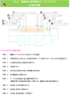
1
METRONAMICA
DOCUMENTATION
Content:
RIKS BV
Layout:
RIKS BV
Illustrations:
RIKS BV
Published by:
RIKS BV
© RIKS BV
This is a publication of the Research Institute for Knowledge Systems (RIKS BV),
Maastrichter Pastoorstraat 14, P.O. Box 463, 6200 AL Maastricht, The Netherlands,
http://www.riks.nl, e-mail: [email protected], Tel. +31(0)433501750, Fax. +31(0)433501751.
Product information
METRONAMICA is a spatial decision support system for urban and regional planning applications. METRONAMICA is
developed in the GEONAMICA software environment. It comes as a stand-alone software application with a user
friendly interface.
METRONAMICA and GEONAMICA are developed by the Research Institute for Knowledge Systems, Maastricht, The
Netherlands. For more information you are kindly requested to contact RIKS BV or visit www.metronamica.nl.
Metronamica documentation
© RIKS BV
Research Institute for Knowledge Systems BV
P. O. Box 463
6200 AL Maastricht
The Netherlands
www.riks.nl
Contents
1. INTRODUCTION....................................................................................................1
2. USER MANUAL......................................................................................................3
2.1
Getting started....................................................................................................3
2.1.1 Computer requirements..............................................................................3
2.1.2 Installing METRONAMICA and accompanying tools..................................4
2.1.3 METRONAMICA directory structure ...........................................................4
2.1.4 MAP COMPARISON KIT directory structure ..............................................5
2.1.5 Starting METRONAMICA ............................................................................5
2.1.6 Screen layout............................................................................................31
2.1.7 System information..................................................................................32
2.1.8 Closing METRONAMICA ..........................................................................33
2.1.9 If you experience problems......................................................................33
2.2
Running the simulation ....................................................................................35
2.2.1 Project file, integrated scenario and sub-scenario....................................35
2.2.2 Opening a project file...............................................................................36
2.2.3 Editing input and displaying output.........................................................38
2.2.4 Saving changes.........................................................................................49
2.2.5 Running a scenario...................................................................................54
2.2.6 Saving results ...........................................................................................57
2.2.7 Tools for analysing results .......................................................................59
2.3
Policy interface ................................................................................................68
2.3.1 Overview of the policy interface..............................................................68
2.3.2 Setting up the drivers ...............................................................................70
2.3.3 Visualising indicators...............................................................................88
2.3.4 Analysing results......................................................................................94
2.4
Modeller interface............................................................................................97
2.4.1 Overview of the system diagram .............................................................97
2.4.2 Model Building Blocks (MBBs)..............................................................98
2.4.3 Connectors and connections ....................................................................98
2.4.4 Dialog windows .......................................................................................99
2.4.5 Individual model components..................................................................99
2.5
The Metronamica menu system .....................................................................159
2.5.1 File menu ...............................................................................................159
2.5.2 Simulation menu ....................................................................................160
2.5.3 Maps menu.............................................................................................160
I
2.5.4 Options menu .........................................................................................162
2.5.5 Windows menu ......................................................................................164
2.5.6 Help menu..............................................................................................164
3. MODEL DESCRIPTION....................................................................................165
3.1
MBB Land Use ..............................................................................................165
3.1.1 Description MBB Land use ...................................................................165
3.1.2 Cellular Automata..................................................................................170
3.1.3 Neighbourhood potential .......................................................................174
3.1.4 Accessibility...........................................................................................175
3.1.5 Suitability...............................................................................................180
3.1.6 Zoning ....................................................................................................182
3.1.7 Transition potential ................................................................................187
3.1.8 Land use .................................................................................................188
3.2
MBB Spatial indicators..................................................................................190
3.2.1 Description MBB Spatial indicators ......................................................190
3.2.2 Cluster indicator.....................................................................................194
3.2.3 Neighbourhood indicator .......................................................................195
3.2.4 Distance indicator ..................................................................................196
3.2.5 Distance to map indicator ......................................................................197
3.2.6 Mask/mapping indicator ........................................................................199
3.2.7 Habitat fragmentation (KOV) indicator.................................................199
3.2.8 Land use change indicator .....................................................................201
3.2.9 Spatial metric indicator ..........................................................................201
3.3
MBB Regional interaction .............................................................................202
3.3.1 Description MBB Regional interaction .................................................202
3.3.2 Activity ..................................................................................................206
3.3.3 National growth .....................................................................................207
3.3.4 Migration................................................................................................208
3.3.5 Attractivity for activity in all sectors .....................................................209
3.3.6 Productivity............................................................................................216
3.3.7 Cell demands per sector .........................................................................218
3.3.8 The sector to land use conversion model block .....................................219
3.4
MBB Transport ..............................................................................................221
3.4.1 Description MBB Transport ..................................................................221
3.4.2 Regional activities to transport zonal activities .....................................224
3.4.3 Local activities to transport zonal activities...........................................225
3.4.4 Urbanization level..................................................................................227
3.4.5 Production and attraction .......................................................................228
3.4.6 Distribution and modal split...................................................................231
3.4.7 Transport assignment .............................................................................233
3.4.8 Transport indicators ...............................................................................242
II
3.4.9 Transport annex 1: Bootstrapping distribution ......................................248
3.4.10
Transport annex 2: Furness Iteration .................................................250
4. METRONAMICA DATA REQUIREMENT....................................................253
4.1
Model specification........................................................................................253
4.1.1 Definition of the region modelled..........................................................253
4.1.2 Base years for which data can be collected ...........................................253
4.1.3 Resolution of the land use model...........................................................254
4.1.4 Length of typical simulation runs ..........................................................254
4.1.5 Land use types modelled at the local level ............................................254
4.1.6 Sectors modelled at the regional level ...................................................254
4.2
Required data and configuration of Metronamica .........................................254
4.3
GIS data for the land use model.....................................................................254
4.3.1 D1 Land use maps..................................................................................255
4.3.2 D2 Base maps required for suitability calculation.................................255
4.3.3 D3 Suitability maps generated with external tool..................................256
4.3.4 D4 Base maps required for zoning calculation ......................................256
4.3.5 D5 Zoning maps generated with external tools .....................................257
4.3.6 D6 Networks ..........................................................................................258
4.3.7 D7 Borders of regions............................................................................258
4.4
Census and other statistical data for the regional model................................258
4.4.1 D8 Population data.................................................................................259
4.4.2 D9 Employment .....................................................................................259
4.5
Additional data for the transport model .........................................................259
4.5.1 Decision for setup ..................................................................................259
4.5.2 Overview data for the transport model ..................................................261
4.5.3 D10 Transport zone map........................................................................261
4.5.4 D11 Roads network maps ......................................................................261
4.5.5 D12 Roads network changes maps ........................................................263
4.5.6 D13 initial trip distribution for car transport and for public transport...263
4.5.7 D14 Other data for public transport .......................................................263
4.5.8 D15 Data for calibrating the transport model ........................................264
APPENDIX A: METRONAMICA RELEASE HISTORY..................................265
III
1. Introduction
Metronamica is RIKS’ Spatial Decision Support System (SDSS) for urban and regional
planning applications. METRONAMICA consists of a dynamic, spatial land use change
model and can optionally include a regional migration model and a transport model for
modelling congestion and traffic pressure on the transport network.
Land use changes are simulated based on a number of different drivers. First there are
external factors such as population growth or the decrease of natural area that determine
the demand for different land uses. Population and jobs are divided over the regions,
based on how attractive these regions are to people and businesses. This attractiveness
depends again on a number of factors such as the existing activity and local
characteristics such as the accessibility. Finally, within each region, the land uses for
every location are determined based on socio-economic factors (e.g., will a business
flourish in this location?), policy options (e.g., are there policy rules in effect that
restrict new housing development in this location?) and biophysical factors (e.g., is the
soil suited for agriculture here?).
METRONAMICA is calibrated on historic land use changes, which is extrapolated to
simulate land use developments into the future. After that, planners can experiment with
scenarios, policy options and external influences such as spatial zoning plans, expansion
of the road network or population growth scenarios, and assess the effect compared to
the baseline scenario. This enables planners to gain insights in possible future land use
developments and the influence of alternative policy measures.
METRONAMICA is developed in the GEONAMICA software environment. It comes as a
stand-alone software application with a user friendly interface. The system includes the
MAP COMPARISON KIT for analysis of model results. Both tools use data formats that
are compatible with standard GIS packages such as ArcGIS.
The METRONAMICA documentation contains four chapters:
Chapter 1 Introduction explains the structure of the METRONAMICA documentation.
Chapter 2 User Manual describes how to use the software of METRONAMICA.
Chapter 3 Model description gives the detailed description for each model used in the
system.
Chapter 4 Metronamica data requirement describes input data and their format required by
METRONAMICA.
Chapter Appendix A: Metronamica release history describes the METRONAMICA release
history.
1
2. User Manual
This chapter describes the user manual of METRONAMICA, a spatial decision support
system built with the GEONAMICA framework. The METRONAMICA is developed to
model, explore and visualize land-use change effects of the different scenarios for urban
and regional planning applications.
This manual contains five the sections:
Section 2.1 “Getting started” explains how to install METRONAMICA on your computer
and how to start the program. It also describes the main features of the graphical user
interface.
Section 2.2 “Running the simulation” contains a step-by-step description of how to run the
simulation in METRONAMICA.
Section 2.3 “Policy interface” describes the steps that a policy user should follow to carry
out an integrated impact assessment with the METRONAMICA system.
Section 2.4 “Modeller interface” describes the interface for a modeller to access the
underlying models and to update data and parameter settings through the system
diagram in METRONAMICA.
Section 2.5 “The Metronamica menu system” offers a systematic description of each
option in the menu system.
Through this documentation, for the convenience of the user, a special arrow symbol
is used in a step-by-step description of how to complete the action that you can follow
along at your computer. For example:
¾ Click Open project on the File menu.
2.1
Getting started
This chapter explains how to install METRONAMICA and its accompanying tools on
your computer and how to start the program. It also describes the main features of the
graphical user interface.
2.1.1
Computer requirements
METRONAMICA runs on personal computers running Microsoft Windows XP and
equipped with modern Intel or Intel compatible processors. It may also run on Windows
Vista and Windows 7, but has only been fully tested on Windows XP. To use
METRONAMICA, your computer should have the following hardware components:
• At least 512 MB of RAM
• A hard disk with at least 1GB free space
3
To use METRONAMICA, you should have the following software packages installed on
your computer:
• Microsoft® Excel (version 2003 or later) (required)
• Microsoft® Picture and fax viewer or Internet explorer (optional)
METRONAMICA is developed for Windows XP. If you experience problems when
installing the METRONAMICA on Windows Vista and Windows 7, please contact us (see
the section If you experience problems).
2.1.2
Installing METRONAMICA and accompanying tools
The following is a step-by-step description of the installation of METRONAMICA. The
installation/uninstallation of METRONAMICA follows standard Windows procedures.
If you have a previous version of the METRONAMICA software installed on your
machine, you will be asked whether you want to uninstall it first. We recommend
uninstalling it. If you want to keep it, make sure to put the latest version of
METRONAMICA in a separate folder. During the installation you may encounter a
message asking whether you want to keep or replace certain files. We recommend
replacing those files for use with METRONAMICA. Keeping the old files may cause the
software to malfunction.
To install Metronamica
¾ Step 1. Start Microsoft Windows XP.
¾ Step 2. Download or copy the Metronamica setup.
¾ Step 3. Double-click on the Metronamica_#.#.#_setup.exe. The #.#.# refers to
the version number of the software installation.
¾ Step 4. Follow the steps on the screen to install the software and data.
¾ Step 5. (Optional) Download the MAP COMPARISON KIT from
http://www.riks.nl/mck. Install it by double-clicking the downloaded file and
follow the steps on the screen.
To uninstall Metronamica
¾ Step 1. Open the Control Panel (this is normally available in the Windows Start
menu). Open ‘Add or Remove Programs’ in the Control Panel. Next click the
‘Change or remove programs’ button in the ‘Add’ or ‘Remove Programs Properties’
dialog window.
¾ Step 2. Select Metronamica from the list of applications and press the
‘Change/Remove’ button.
¾ Step 3. The Confirm File Deletion dialog window will open. Press the ‘OK’ button
to confirm that you want to remove Metronamica and all its files from your hard
disk.
¾ Step 4. Repeat the steps 1 to 3 to uninstall the MAP COMPARISON KIT.
2.1.3
METRONAMICA directory structure
By default METRONAMICA is installed in the directory C:\Program Files\Geonamica.
Two sub-directories are created: Metronamica and Map Comparison Kit.
4
By default example data for METRONAMICA is installed in C:\Documents and
Settings\My Documents \User\Metronamica. The example data in the current version
Metronamica is Randstad (SL).
• Randstad (SL): an example case for Metronamica SL, which includes only the
land use model.
The directories for each METRONAMICA project contain typically the following subdirectories and files.
• Animations: animation maps generated during a simulation
• Data: base maps required to run a simulation and the intermediate output maps
for the current simulation year
• Legends: map legends
• Log: logged maps generated during a simulation
• *.geoproj: the project file of METRONAMICA created for the specific case. The
project file Randstad.geoproj is made for the purpose of demonstration. The
project file Randstad_exercises.geoproj is made for the purpose of exercises. For
more information about exercises, we refer to the document
Metronamica_Introduction_Exercise.pdf under C:\Documents and Settings\My
Documents \User\Metronamica.
2.1.4
MAP COMPARISON KIT directory structure
By default the MAP COMPARISON KIT is installed in the directory C:\Program
Files\Geonamica.
By default the additional data for the MAP COMPARISON KIT are installed in
C:\Documents and Settings\User\My Documents\Geonamica\MCK. There are four subdirectories in this folder:
• Examples: examples developed for the MAP COMPARISON KIT
• Palettes: palettes legends for the MAP COMPARISON KIT
2.1.5
Starting METRONAMICA
Once installed, you can start the METRONAMICA application as follows:
¾ Click the ‘Start’ button on the Windows taskbar.
¾ Go to All Programs → Geonamica → Metronamica.
¾ Click on METRONAMICA.
Importing the licence file
The first time you start METRONAMICA a dialog window will appear asking you to
install a licence file for METRONAMICA. Once a license is installed, the software will
skip this step, unless the installed license has expired.
¾ Click the OK button on the message window.
A dialog window will open allowing you to navigate to the folder where you put the
licence file for METRONAMICA that you have received.
¾ Open the licence file with the extension .lic.
Each time you start METRONAMICA, the About window appears (see the section About).
5
¾ Click the OK button on the About window.
Creating a new project file for Metronamica SL
Selecting the project configuration
METRONAMICA consists of a dynamic, spatial land use change model and can
optionally include a regional migration model and a transport model for modelling
congestion and traffic pressure on the transport network. The availability of the versions
depends on the licence file that you are using.
• Metronamica SL: containing only the land use model as a single layer
• Metronamica ML: containing the land use model and the regional model as
multiple layers
• Metronamica LUT: containing the land use model, the regional model and the
transport model
After you click the OK button on the About window, the ‘Open project file’ dialog window
opens. You are going to create a new project file.
¾ Click the ‘Cancel’ button on the ‘Open project file’ dialog window.
¾ Click the ‘New project’ command on the File menu. The ‘New Metronamica project
wizard’ window opens.
6
¾ Click the Next button. The ‘Project configuration’ dialog window opens to ask you
for which type of Metronamica you want to create a new project file.
¾ Click the radio button next to Metronamica SL.
¾ Determine if you want to include the zoning tool in the new project file. For
more information about the zoning tool, see the section Policy measures - zoning.
• The zoning tool will be included in the new project file if you select the check
box in front of ‘Use zoning tool’. In two steps of this step, a new dialog window
named ‘Enter the zoning tool parameters’ will appear to ask you to set the zoning
tool parameters. For more information, see the section Entering the zoning tool
parameters.
• The zoning tool will be excluded in the new project file if you unselect the check
box in front of Use zoning tool. The ‘Enter the zoning tool parameters ‘dialog
window mentioned above will not appear and the step of setting the zoning tool
parameters will be skipped.
¾ Determine if you want to include the suitability tool in the new project file. For
more information about the suitability tool, see the section Suitability.
¾ Click the ‘Next’ button. Another dialog window opens to ask you enter the basic
project parameters.
7
Entering the basic project parameters
¾ In the text boxes next to Simulation start year, fill in the start year of the
simulation in the project file that you want to create. You can not change the
start year of simulation via the user interface after you create the project file.
¾ In the text boxes next to Simulation end year, fill in the end year of the simulation
in the project file that you want to create.
Note that the end year of simulation should be after the start year of the simulation.
Otherwise, an error message as depicted below will appear when you click the Next
button.
You can change the end year of the simulation via the user interface after the project is
created. For more information, see the section Simulation menu.
¾ Click the browse button next to ‘Region boundaries map’. The ‘Open’ dialog
window opens.
¾ Navigate the region map that you want to import and double-click on it.
Note that the region map that you import from here should be a raster map. The outside
of modelling area should have value 0.
8
After you import the raster region map, all the values on this map are listed in the table
with the default region names.
If you do not have a licence which allows you to create a new METRONAMICA project
for the specific region, you will get an error message. If you still want to set up a new
project file for this region, please contact RIKS for more information (see the section If
you experience problems).
You can edit the region name by clicking on the cell of interesting and entering a new
name.
Press the Next button. A new wizard dialog window opens to ask you entering the basic
land use model parameters.
9
Entering the basic land use model parameter
The map size and cell size are displayed on the top of this window for your information,
which are generated from the region map that you imported in the previous step.
Note that in Metronamica, all raster maps such as land use maps, region maps, suitability
maps, zoning maps should be strictly comparable: they must be of identical map size
(i.e. cover the same area), resolution (cell size), and origin (the lower-left x-coordinate
and the lower-left y-coordinate).
¾ Click on the browse button next to ‘Initial land use map’. The ‘Open’ dialog
window opens.
¾ Navigate the initial land use map that you want to import and double-click on it.
You have been imported the initial land use map to the new project.
Once the initial land use map is imported, the path of the map is displayed in the text
box next to Initial land use map. At the same time, the information on the initial land use
map appears in the table under Land use classes in a default way.
10
¾ You need to edit names for each land use class by clicking on the text box of
interesting in the ‘Class name’ column and entering a new name.
¾ You can edit the legend for each land use class by clicking on the cell of interest
in the ‘Legend colour’ column. The ‘Colors’ dialog window opens. Select the
colour of interest and press the OK button in the Colors dialog window. The new
selected colour is displayed for the land use of interest.
You can also edit the legends for the land use map via the user interface after setting up
the METRONAMICA project. For more information, see the section Legend editor.
In Metronamica, the land use is classified in types or categories, some of which are
modelled dynamically while others remain static.
• Vacant states are classes that are only changing as a result of other land use
dynamics.
• Functions are land use classes that are actively modelled.
• Features are land use classes that are not supposed to change in the simulation.
For more information about the land use states, see the section Land use classes.
¾ You need to determine the land use type for each land use in this step. Click on
the dropdown list in the Type column for the land use of interest. Select one of
the types from the list.
¾ You need to determine the land use group for each land use for creating the
environmental indicators. Click on the dropdown list in the ‘Environmental group’
column for the land use of interest. Select one of the groups from the list: urban,
forest, natural (non-forest) and other.
¾ You need to determine the land use group for each land use for creating the
social-economic indicators. Click on the dropdown list in the ‘Social-economic
group’ column for the land use of interest. Select one of the groups from the list:
work, residential, recreation and other.
For more information about the indicators, see the section Visualising indicators.
11
The number of land use classes is taken from the initial land use map you imported. In
order to facilitate the scenario study, METRONAMICA allows you to add additional land
use classes as land use feature. To do so,
¾ Go to the last empty line of the ‘Land use classes’ table.
¾ Click the cell in the ‘Class name’ column and a name for the land use feature that
you want to add.
¾ Press the Enter key on your key board. The Type of the newly added land use
will be set automatically as Feature. You could not add additional land use
classes for vacant or function.
A new empty line appears at the bottom of the ‘Land use classes’’. You could add
another new land use feature by repeating the steps described above.
¾ Click on the ‘Next’ button on the ‘Enter the basic land use model parameters’ dialog
window.
Entering the zoning tool parameters
If you have not selected the check box in front of Use zoning tool’, this step will be
skipped and a new dialog window opens to ask you entering the infrastructure networks.
For more information, see the section Entering the infrastructure networks.
If you have selected the check box in front of Use zoning tool, the dialog window ‘Enter
the zoning tool parameters’ depicted as below appears. Four default zoning states are
listed in the table with their default numerical value.
In this wizard step, it is very important to define the number of zoning states and their
names. You could not change these via the user interface after setting up the application.
Once the number of zoning states and their names are set in this step, you can also
modify their numerical values after setting up the application. For more information
about how to reset the numerical values, see the section Zoning.
¾ You can edit the name of the zoning states and their numerical value by clicking
in the cell of interest and entering a new name and/or a new value.
¾ You can add a new zoning state and its numerical value in the last empty line.
¾ You can delete a zoning state and its numerical value by selecting the
correspondent line and press the Delete key on your key board.
12
¾ Press the ‘Next’ button on the ‘Enter the zoning tool parameters’ dialog window. A
new dialog window opens to ask you entering the infrastructure networks.
Entering the infrastructure networks
You can import the infrastructure networks from this step and you can also add or
remove any infrastructure networks via the user interface after setting up the project
(see the section Accessibility for more information).
To import the infrastructure networks in this step
¾ Click on the ‘Add’ button. The ‘Add new map’ dialog window opens.
¾ Enter the name of the infrastructure network in the text box next to ‘Map name’.
¾ Click the browse button next to ‘Filename’. The Open dialog window opens.
Navigate the infrastructure network map stored that you want to import and
double-click on it.
Note that the infrastructure network should be in *.shp or *.bin format and contain a
field named “Acctype”. For the network shape file in point format, you need to convert
it to polyline format before you import it as an infrastructure layer.
¾ Press the OK button in the ‘Add new map’ dialog window. The newly added
infrastructure network appears on the list.
13
If you have multiple network layers (e.g. roads network, railway network or stations),
repeat the steps above to add more layers to the list.
¾ Select one of the infrastructure networks. The ‘Edit’ button and ‘Remove’ button
on the right side of the window become available.
¾ You can edit the map name and change the file via ‘Edit’ button and you can
delete the selected map by clicking the Remove button.
¾ Click the ‘Next’ button on the button. The ‘Configure accessibility settings’ dialog
window opens, where the values of Acctype in all the networks that you
imported are listed in the table.
14
¾ You need to enter the accessibility type name for each value in the text boxes of
‘Accessibility type name’ column.
¾ Click the ‘Next’ button at the bottom. A new dialog window opens asking you to
fill in the name and the path for the new project file.
Finalizing the setup of project
This is the last step of the new project wizard.
¾ Specify the name of your project in the Project name box.
¾ Specify the location where it should be stored. Metronamica will automatically
create a new sub-folder with your project name in the folder selected by you. All
the data you have imported in the new project wizard will be copied there. You
can select any location on a hard dist, USB stick or network drive.
¾ You can selecte the ‘Support large maps’ check box if you want to create a
project that contains large maps.
For projects where the option ‘Support large maps’ is enabled, METRONAMICA will
cache map data on the hard disk, causing it to run slower. Therefore, the option is not
advised unless you experience problems without it. The new project wizard will
automatically select the check box, if the expected memory usage based on the
information you have entered exceeds a certain threshold. If the check box is
automatically selected and you clear it, there is a risk that METRONAMICA may crash
while using the new project. If you select the check box, you may want to change the
cache folder for map data – see section Raster map cache folder.
¾ Click the ‘Finish’ button when you are ready to save your new project to the
specified location. Your new project will be opened automatically.
15
The METRONAMICA will be started and you will see the METRONAMICA - ###
application window on your screen, where “###” is the project name that you entered in
the last step.
After the project is set up, all the maps that are used during setting up the project file
will be copied in folder Data.
Creating a new project file for Metronamica ML
Selecting the project configuration
METRONAMICA consists of a dynamic, spatial land use change model and can
optionally include a regional migration model and a transport model for modelling
congestion and traffic pressure on the transport network. The availability of the versions
depends on the licence file that you are using.
• Metronamica SL: containing the land use model as a single layer
• Metronamica ML: containing the land use model and the regional model as
multiple layers
• Metronamica LUT: containing the land use model, the regional model and the
transport model
After you click the OK button on the About window, the ‘Open project file’ dialog window
opens. You are going to create a new project file.
16
¾ Click the ‘Cancel’ button on the ‘Open project file’ dialog window.
¾ Click the ‘New project’ command on the ‘File’ menu. The ‘New Metronamica project
wizard’ window opens.
¾ Click the Next button. The ‘Project configuration’ dialog window opens to ask you
for which type of Metronamica you want to create a new project file.
¾ Click the radio button next to Metronamica ML.
¾ Determine if you want to include the zoning tool in the new project file. For
more information about the zoning tool, see the section Policy measures - zoning.
• The zoning tool will be included in the new project file if you select the check
box in front of Use zoning tool. In two steps of this step, a new dialog window
named Enter the zoning tool parameters will appear to ask you to set the zoning
tool parameters. For more information, see the section Entering the zoning tool
parameters.
• The zoning tool will be excluded in the new project file if you do not select the
check box in front of ‘Use zoning tool’. The ‘Enter the zoning tool parameters’
17
dialog window mentioned above will not appear and the step of setting the
zoning tool parameters will be skipped.
¾ Determine if you want to include the suitability tool in the new project file. For
more information about the suitability tool, see the section Suitability.
¾ Click the Next button. Another dialog window opens to ask you enter the basic
project parameters.
Entering the basic project parameters
¾ In the text boxes next to Simulation start year, fill in the start year of the
simulation in the project file that you want to create. You can not change the
start year of simulation via the user interface after you create the project file.
¾ In the text boxes next to Simulation end year, fill in the end year of the simulation
in the project file that you want to create.
Note that the end year of simulation should be after the start year of the simulation.
Otherwise, an error message as depicted below will appear when you click the Next
button.
18
You can change the end year of the simulation via the user interface after the project is
created. For more information, see the section Simulation menu.
¾ Click the browse button next to ‘Region boundaries map’. The ‘Open’ dialog
window opens.
¾ Navigate the region map that you want to import and double-click on it.
Note that the region map that you import from here should be a raster map. The outside
of modelling area should have value 0.
After you import the raster region map, all the values on this map are listed in the table
with the default region names.
If you do not have a licence which allows you to create a new METRONAMICA project
for the specific region, you will get an error message. If you still want to set up a new
project file for this region, please contact RIKS for more information (see the section If
you experience problems).
19
You can edit the region name by clicking on the cell of interesting and entering a new
name.
Press the Next button. A new wizard dialog window opens to ask you entering the basic
land use model parameters.
Entering the basic land use model parameter
The map size and cell size are displayed on the top of this window for your information,
which are generated from the region map that you imported in the previous step.
Note that in Metronamica, all raster maps such as land use maps, region maps, suitability
maps, zoning maps should be strictly comparable: they must be of identical map size
(i.e. cover the same area), resolution (cell size), and origin (the lower-left x-coordinate
and the lower-left y-coordinate).
¾ Click on the browse button next to Initial land use map. The ‘Open’ dialog
window opens.
¾ Navigate the initial land use map that you want to import and double-click on it.
You have been imported the initial land use map to the new project.
20
Once the initial land use map is imported, the path of the map is displayed in the text
box next to Initial land use map. At the same time, the information on the initial land use
map appears in the table under Land use classes in a default way.
¾ You need to edit names for each land use class by clicking on the text box of
interesting in the ‘Class name’ column and entering a new name.
¾ You can edit the legend for each land use class by clicking on the cell of interest
in the ‘Legend colour’ column. The ‘Colors’ dialog window opens. Select the
colour of interest and press the OK button in the Colors dialog window. The new
selected colour is displayed for the land use of interest.
You can also edit the legends for the land use map via the user interface after setting up
the METRONAMICA project. For more information, see the section Legend editor.
In Metronamica, the land use is classified in types or categories, some of which are
modelled dynamically while others remain static.
21
•
Vacant states are classes that are only changing as a result of other land use
dynamics.
• Functions are land use classes that are actively modelled.
• Features are land use classes that are not supposed to change in the simulation.
For more information about the land use states, see the section Land use classes.
¾ You need to determine the land use type for each land use in this step. Click on
the dropdown list in the Type column for the land use of interest. Select one of
the types from the list.
¾ You need to determine the land use group for each land use for creating the
environmental indicators. Click on the dropdown list in the ‘Environmental group’
column for the land use of interest. Select one of the groups from the list: urban,
forest, natural (non-forest) and other.
¾ You need to determine the land use group for each land use for creating the
social-economic indicators. Click on the dropdown list in the ‘Social-economic
group’ column for the land use of interest. Select one of the groups from the list:
work, residential, recreation and other.
For more information about the indicators, see the section Visualising indicators.
The number of land use classes is taken from the initial land use map you imported. In
order to facilitate the scenario study, METRONAMICA allows you to add additional land
use classes as land use feature. To do so,
¾ Go to the last empty line of the ‘Land use classes’ table.
¾ Click the cell in the ‘Class name’ column and a name for the land use feature that
you want to add.
¾ Press the Enter key on your key board. The Type of the newly added land use
will be set automatically as Feature. You could not add additional land use
classes for vacant or function.
A new empty line appears at the bottom of the ‘Land use classes’ table. You could add
another new land use feature by repeating the steps described above.
¾ Click on the Next button on the ‘Enter the basic land use model parameters’ dialog
window.
22
Entering the zoning tool parameters
If you have not selected the check box in front of Use zoning tool, this step will be
skipped and a new dialog window opens to ask you entering the infrastructure networks.
For more information, see the section Entering the infrastructure networks.
If you have selected the check box in front of ‘Use zoning tool’, the dialog window ‘Enter
the zoning tool parameters’ depicted as below appears. Four default zoning states are
listed in the table with their default numerical value.
In this wizard step, it is very important to define the number of zoning states and their
names. You could not change these via the user interface after setting up the application.
Once the number of zoning states and their names are set in this step, you can also
modify their numerical values after setting up the application. For more information
about how to reset the numerical values, see the section Zoning.
¾ You can edit the name of the zoning states and their numerical value by clicking
in the cell of interest and entering a new name and/or a new value.
¾ You can add a new zoning state and its numerical value in the last empty line.
¾ You can delete a zoning state and its numerical value by selecting the
correspondent line and press the Delete key on your key board.
¾ Press the ‘Next’ button on the ‘Enter the zoning tool parameters’ dialog window. A
new dialog window opens to ask you entering the infrastructure networks.
Entering the infrastructure networks
You can import the infrastructure networks from this step and you can also add or
remove any infrastructure networks via the user interface after setting up the project
(see the section Accessibility for more information).
23
To import the infrastructure networks in this step
¾ Click on the ‘Add’ button. The ‘Add new map’ dialog window opens.
¾ Enter the name of the infrastructure network in the text box next to ‘Map name’.
¾ Click the browse button next to Filename. The ‘Open’ dialog window opens.
Navigate the infrastructure network map stored that you want to import and
double-click on it.
Note that the infrastructure network should be in *.shp or *.bin format and contain a
field named “Acctype”. For the network shape file in point format, you need to convert
it to polyline format before you import it as an infrastructure layer.
¾ Press the OK button in the ‘Add new map’ dialog window. The newly added
infrastructure network appears on the list.
If you have multiple network layers (e.g. roads network, railway network or stations),
repeat the steps above to add more layers to the list.
24
¾ Select one of the infrastructure networks. The ‘Edit’ button and ‘Remove’ button
on the right side of the window become available.
¾ You can edit the map name and change the file via ‘Edit’ button and you can
delete the selected map by clicking the ‘Remove’ button.
¾ Click the ‘Next’ button on the button. The ‘Configure accessibility settings’ dialog
window opens, where the values of Acctype in all the networks that you
imported are listed in the table.
¾ You need to enter the accessibility type name for each value in the text boxes of
‘Accessibility type name’ column.
¾ Click the ‘Next’ button at the bottom. A new dialog window opens to you
continuing the configuration of the regional model.
Specifying the sectors of the regional model
The first step in setting up the regional interaction model is to list the sectors that will be
modelled. There are three types of sectors: population sectors model the number of
people in each region; economic sectors model the number of jobs in each region; and
area sectors simply specify a land use demand for each region. When you enter the
25
name of a sector in the first column of the table, a list will be shown in the second
column in which you can select the sector type. A new row will be inserted at the
bottom of the table where you can enter the next sector.
The setup of the regional model starts from this step
¾ Enter the sector name in the text box in the ‘Sector name’ column.
¾ Press Enter on your keyboard. A dropdown list arrow appears in the column of
‘Sector type’.
¾ Select the sector type from the dropdown list in the ‘Sector type’ column for the
newly entered sector.
¾ Repeat the steps above till specifying all the sectors.
26
¾ Click the Next button. A new wizard dialog window opens to ask you linking the
land use functions to sectors.
Linking land use functions to sectors
The second step in setting up the regional interaction model is to link the sectors to the
land use functions. Area sectors must be linked one-to-one to a land use function.
Population and economic sectors can be linked to land use function with a many-tomany relation.
The available land use functions are listed in the ‘Land use functions’ column of this
dialog window, which were determined in step Entering the basic land use model parameter.
In the ‘Corresponding sector’ column, all the sectors available are listed on the dropdown
list, which were the sector names determined in step Specifying the sectors of the regional
model. By default, the wizard shows a table in which sectors and land use functions can
be linked one-to-one.
¾ Click the dropdown list in the ‘Corresponding sector’ column.
¾ Select the corresponding sector from the list next to each land use function.
If you would like to create a more complex links than only one-to-one,
27
¾ Click the ‘Show advanced settings’ button. The table will transform to show a
matrix of values between 0 and 1.
¾ Change the values to specify the function to sector correspondence, thereby
adhering to the following requirements:
• All values must be larger than or equal to 0 and smaller than or equal to 1.
• The values for each land use function must sum to 1 (with 12 digits precision).
• Each area sector must be linked to exactly one land use function with the value 1,
and 0 for all other land use functions.
• The values for each sector must sum to a value larger than 0.
You can still specify the matrix for the links via the user interface after the project is set
up.
¾ Click the Next button. A new wizard dialog window opens to ask you entering
initial data for the regional model.
Entering initial jobs or population per sector
The third and last step in setting up the regional interaction model is to specify the
number of people or jobs in the simulation start year for each population and economic
sector, respectively. The values you enter can be decimal numbers – that is, they do not
need be integral. However, you cannot enter negative numbers.
All the regions available are listed in this dialog window, which were determined in step
Entering the basic project parameters. The default values for initial jobs or population per
sector per region are set to zero.
¾ Give the initial jobs and population per sector per region by double-clicking the
cell of interest and entering a new value. You can copy and past these data from
Excel sheet that you prepared.
It is easier to enter the initial from the wizard. However, if your data is not ready, you
can skip this step by pressing the Next button. Then you can still specify the initial data
for the regional model via the user interface.
¾ Click the Next button. The last new wizard dialog window opens.
28
Finalizing the setup of project
This is the last step of the new project wizard.
¾ Specify the name of your project in the Project name box.
¾ Specify the location where it should be stored. Metronamica will automatically
create a new sub-folder with your project name in the folder selected by you. All
the data you have imported in the new project wizard will be copied there. You
can select any location on a hard dist, USB stick or network drive.
¾ You can selecte the ‘Support large maps’ check box if you want to create a
project that contains large maps.
For projects where the option ‘Support large maps’ is enabled, METRONAMICA will
cache map data on the hard disk, causing it to run slower. Therefore, the option is not
advised unless you experience problems without it. The new project wizard will
automatically select the check box, if the expected memory usage based on the
information you have entered exceeds a certain threshold. If the check box is
automatically selected and you clear it, there is a risk that METRONAMICA may crash
while using the new project. If you select the check box, you may want to change the
cache folder for map data – see section Raster map cache folder.
¾ Click the ‘Finish’ button when you are ready to save your new project to the
specified location. Your new project will be opened automatically.
29
The METRONAMICA will be started and you will see the METRONAMICA - ###
application window on your screen, where “###” is the project name that you entered in
the last step.
After the project is set up, all the maps that are used during setting up the project file
will be copied in folder Data.
Opening the project file
If you have already had your project file *.geoproj on your computer and you have
imported your licence file for METRONAMICA, you can open your project file as
following steps. For more information about how to import the licence file, see the
section Importing the licence file. For more information about how to create a new project,
see the section Creating a new project file for Metronamica SL or see the section Creating a
new project file for Metronamica ML.
¾ Go to Start → All programs → Geonamica → Metronamica.
¾ Click the Metronamica icon.
Each time you start Metronamica, the About window appears (see the section About).
¾ Click the OK button on the About window. The ‘Open project file’ dialog window
opens.
¾ Navigate to the project file that you want to open and double-click on it.
If the project file you want to open is created with an older version of Metronamica, a
message window will appear to ask you whether to upgrade the project file to the
current version of software.
¾ Click the ‘No’ button if you still want to be able to open the project with an
earlier version of the software.
¾ Click the ‘Yes’ button to upgrade the project file automatically. Then you can
open it with the current version of Metronamica. You will no longer be able to
open the project with an earlier version of the software.
METRONAMICA will be started and you will see the METRONAMICA - ### application
window on your screen, where “###” is the project file name that you selected.
30
2.1.6
Screen layout
When you start METRONAMICA, the application window opens immediately. This is the
window in which you will run your simulations. You can arrange windows as you like
in the application window. Before a project file has been opened, the window is empty
except for its Status bar, Toolbar and Menu bar. The different components of this
window will be described in the next paragraphs.
Menu bar
Toolbar
Status bar
Application Window
Menu bar
The Menu bar provides access to various functions in METRONAMICA. The menus are
summarised in the table below. Each menu item is described in detail in the section The
Metronamica menu system.
Use this menu
File
Simulation
Maps
Options
Window
Help
To …
Manage your project files
Control the simulation
Select and view maps
Customise the workspace and select types of output
Manage your windows on the screen
Look up the system information and find help documentation
Toolbar
The Toolbar gives faster access to some of the more frequently used functionality. Each
item on the toolbar is described in the table below.
Item
Function
Open a project file from the disk.
Save the opened project file to disk.
31
Item
Function
Displays the active integrated scenario. The dropdown list shows all the
available integrated scenarios. You can load an integrated scenario by
selecting it from the dropdown list.
Advance the simulation with one simulation step.
Advance the simulation till the next pause is reached.
Stop the simulation after the current step is finished.
Reset the simulation to the initial year.
Displays the current simulation time whenever a project is open.
Status bar
The Status bar is displayed at the bottom of the application window. It contains
different sections that provide different kinds of information:
• The leftmost section provides general information. When you navigate through
the menu, it describes the selected menu item.
• The second section from the left provides local information when you move the
mouse over a map. For a raster map, it lists the cell index and the value in that
cell. For network maps, it lists the x and y coordinates of the location.
• The third section from the left displays a progress bar while the model is
calculating.
• The rightmost sections of the Status bar indicate which of the following keys are
latched down: the Caps Lock key (CAP), the Num Lock key (NUM), or the
Scroll Lock key (SCRL).
2.1.7
System information
The different commands in the Help menu allow you to look up the system information
about METRONAMICA. For more information see the section Help menu.
Help
Click Index on the Help menu (or press the F1 key) to open the on-line help file of
Metronamica. Use the Contents tab on the left side of the Metronamica documentation
window to navigate to the topic that you want help on. You can also use the Search tab
to find the relevant section in the user manual. If these tabs are not displayed, click the
‘Show’ button at the top of the Metronamica documentation window.
Licence
Click Licence on the Help menu to get the licence information in the Installed licenses
window. All licences for the Geonamica-based software installed on your computer will
be listed in the table. You can import a licence file (with extension .lic) by clicking the
‘Read a licence file’ button. To remove a license, click the ‘Open license folder’ button and
remove the files with the license name you want to remove from the folder. You need to
restart the application for the changes to take effect. There is no need to remove existing
licenses before installing a new one.
32
Checking for updates
Click ‘Check for updates’ on the Help menu to check if you are using the latest version of
Metronamica. If a newer version is available, the system will tell you how to get it.
About
Click on About on the Help menu to open the About window. Here, you can find the
copyright notice and version number of METRONAMICA. The latter is important if you
need assistance with the software (see the section If you experience problems) or when
you request an update of the software.
Version number
2.1.8
Closing METRONAMICA
You can close METRONAMICA by clicking Exit on the File menu. If you have a project
file open, the application may ask whether you want to save your changes before
closing.
Click the ‘Yes’ button to save your changes, click the ‘No’ button to discard your
changes and close METRONAMICA or click the ‘Cancel’ button to keep METRONAMICA
open. More information on saving changes is available in the section Saving changes.
2.1.9
If you experience problems
If you experience problems installing or running METRONAMICA, please contact RIKS
with the version number of the application (see the section About):
Research Institute for Knowledge Systems bv.
To the attention of Hedwig van Delden
P.O. Box 463, 6200 AL Maastricht, The Netherlands
Tel: +31 (43) 3501750
33
Fax: +31 (43) 3501751
E-mail: [email protected]
Website: www.riks.nl
34
2.2
Running the simulation
This section describes the primary steps of running a simulation with METRONAMICA:
Opening a project file, editing input and displaying output, saving changes, running a
scenario, saving results and analysing results.
2.2.1
Project file, integrated scenario and sub-scenario
It is important to understand how the input data/files and parameters that are required to
run models in the system are organized in METRONAMICA. We use the terms project
file, integrated scenario and sub-scenario to describe the different levels of data and file
management and parameter value settings.
In the context of this document a scenario is considered to be a set of values for each
driver in METRONAMICA (for more information on drivers in Metronamica, see the
section Setting up the drivers). In particular, you can make scenarios for each of the
drivers that are accessible through the main window. For example in the external factors
you can define increased trend for area of forest and call this scenario increased forest.
When you want to run a simulation in order to investigate the effects of a scenario, you
will have to select exactly one scenario for each of the drivers in METRONAMICA. This
combination would also be named a scenario according to the definition of the term
given above, but of course that is a recipe for confusion. To avoid such confusion we
will qualify the term scenario to mean one of two things:
• A sub-scenario is a set of values for one of the drivers in METRONAMICA that
defines a possible future development of that driver.
• An integrated scenario is a combination of one sub-scenario for each driver in
METRONAMICA that together define a possible overall future development.
This means that the increased forest scenario mentioned above is a sub-scenario and that
an integrated scenario defines all the values for all the drivers that are needed in order to
perform a simulation run. The selected integrated scenario on the toolbar is called the
active integrated scenario.
It should be noted that only sub-scenarios store values for each driver; integrated
scenarios do not store values themselves as they are just a collection of sub-scenarios.
Also, sub-scenarios can exist outside of integrated scenarios – e.g. several predefined
sub-scenarios for area demands, though initially only one of them is selected in an
integrated scenario.
A project file is used to configure various parts of the simulation and it contains
references to all the files that are required to run models in the system. The project file
used in METRONAMICA has the extension *.geoproj. A project file contains at least one
integrated scenario. The locations of input data and files and parameter values of all
integrated scenarios can be stored in a single project file. A project file must have at
least one sub-scenario specified for each driver. At most one sub-scenario per driver can
be indicated as the baseline scenario. All sub-scenarios created in METRONAMICA are
editable. See the section Saving changes for more information on how to save a subscenario, integrated scenario or project file.
For Metronamica SL, a sub-scenario is composed of:
35
•
Land use demand scenario: related to the total land use demand that you can
access via Drivers → External factors → Total demand.
• Infrastructure scenario: related input data/files for infrastructure networks that
you can access via Drivers → Policy measures → Driver: Infrastructure.
• Zoning scenario: related input data/files and parameters for zoning regulation
that you can access via Drivers → Policy measures → Driver: Zoning.
For Metronamica ML, a sub-scenario is known as:
• Area-demand scenario: related to the demand for each area sector per region that
you can access via Drivers → External factors → Trend → Area of ###, where ###
is the name of area sector.
• Socio-economic trend scenario: related to the trend of number of people and jobs
for population sector and for economic sector per region that you can access via
Drivers → External factors → Trend → Population in ### or Jobs in ***, where ### is
the name of population sector and *** is the name of economic sector.
• Infrastructure scenario: related input data/files for infrastructure networks that
you can access via Drivers → Policy measures → Driver: Infrastructure.
• Zoning scenario: related input data/files and parameters for zoning regulation
that you can access via Drivers → Policy measures → Driver: Zoning.
For Metronamica LUT, a sub-scenario is known as:
• Area-demand scenario: related to the demand for each area sector per region that
you can access via Drivers → External factors → Trend → Area of ###, where ###
is the name of area sector.
• Socio-economic trend scenario: related to the trend of number of people and jobs
for population sector and for economic sector per region that you can access via
Drivers → External factors → Trend → Population in ### or Jobs in ***, where ### is
the name of population sector and *** is the name of economic sector.
• Zoning scenario: related input data/files and parameters for zoning regulation
that you can access via Drivers → Policy measures → Driver: Zoning.
• Mobility growth scenario: related parameters for the mobility growth that you
can access via Drivers → External factors → Trend → Transport.
• Private transport scenario: related input data/files and parameters for the private
transport that you can access via Drivers → Policy measures → Driver: Transport
→ Car transport costs and Transport network changes.
• Public transport scenario: related input data and parameters for the public
transport that you can access via Drivers → Policy measures → Driver: Transport
→ Show/Edit public transport data button.
2.2.2
Opening a project file
In the section Getting started we explained how to install and start METRONAMICA. We
assume from now on that you have read this information, that you have successfully
installed METRONAMICA on your computer and you have knowledge of the different
terms introduced.
36
Opening an existing project file
¾ Open Metronamica if it is not already open – see the section Starting Metronamica.
¾ Click the ‘Open’ button on the toolbar if the ‘Open project file’ window is not
already open.
¾ Navigate to the folder where you installed the Metronamica data and project
files. By default, this is the folder Geonamica\Metronamica inside My
Documents.
¾ Select the geo project file and click the Open button.
Once all files have been loaded, two windows appear in the application window: the
Main window and the Land use map. As you will need to use these windows most of the
time, you cannot close these windows to prevent doing so accidentally. If they are in
your way, click the ‘Minimize’ button on the window and it will move to the bottom of
the application window.
Main window
The Main window is organised in tabs and pages, which are displayed on the left side of
the window. The Main window has 4 tabs: Drivers, Scenarios, Indicators and Analysis.
Each tab has one ore more pages, which are displayed as icons when you click on a tab.
Click on an icon to display a page in the right side of the window, called the content
pane.
Page
Content pane
Tabs
The Main window provides access to the policy user interface and the modeller interface.
The section 2.3 Policy interface and the section 2.4 Modeller interface provide detailed
descriptions of interface for these two types of users.
37
2.2.3
Editing input and displaying output
The models incorporated in METRONAMICA use and compute various forms of input
and output data: spatial, temporal and tabular. These are represented in the graphical
user interface in different ways to best fit the nature of the data. You will be able to find
the following elements in the user interface: maps, graphs, time series, single values and
tables. The following sub-sections describe how to edit input and display output for
each of these elements.
Map window
Since all map windows in METRONAMICA work the same way, we will use the Land use
map window that is opened when you open a project in METRONAMICA as an example. A
Map window is split into 5 areas, called panes as depicted below. Panes are separated
from each other by means of splitter bars. You can move the splitter bars to change the
size of a pane.
Beware: opened maps windows are updated while a scenario runs. This consumes
processing time and will slow down the overall program.
Legend pane
Overview pane
Layer visibility button
Map pane
Layer manager pane
Tools pane
Overview pane
The overview pane displays the entire modelled region. When the map is zoomed in, a
rectangle is displayed that indicates the area displayed in the map pane. You can drag
this rectangle to move the view of the map.
38
Map pane
The map pane in the Land use map window displays the land use map for the current
simulation year. This is a raster map that displays the predominant land use for each cell.
When a simulation is running, the Land use map window will be updated after each time
step.
Right-clicking inside the map pane will display a context menu. Click ‘Cell information’
on this menu to list the land use and district in the exact cell you right-clicked on. You
can also access the same information by using the Inspect tool – see the section Grid
tools.
Double-clicking on the map pane of the Land use map window (this does not work for
other map windows) opens the ‘Contingency table Land use map and Regions map’
window that shows the surface area of each land use in each region – see the image
below. You can select the unit for the surface area from the ‘Display values in’ list. If you
select the ‘Include cells outside modelling area’ checkbox, the land use outside the
modelling area will be displayed in the first column. Otherwise, these values will be
zero. The last row and column in the table display the totals.
Legend pane
The legend pane is displayed in the upper-left portion of the Map window. It shows the
legend of the map selected in the layer Manager pane (explained below). For example, if
you select a land use map, the legend pane shows the land use legend. Double-click in
the legend pane to change the legend that is displayed – see the section Legend editor.
Land uses are subdivided into 3 types: Vacant, Function, Feature. In the land use
legend, the Vacant land uses appear at the top of the list, the Function land uses appear
in the middle of the list and are underlined, and the Feature land uses appear at the
bottom of the list. The 3 different land use types are explained in the section Land use
classes.
39
Layer manager pane
The layer manager pane is displayed in the upper-right portion of a map window. You
can select a layer by clicking on its name. This will display the legend for the layer and
allow you to edit the layer (if possible) – see the section Grid tools and Network tools.
You can show or hide a layer by clicking on the layer visibility button in the layer
manager pane.
Button
Function
Layer is visible
Layer is hidden
Tools pane
The tools pane is displayed in the lower-right portion of the Map window. It shows the
tools for viewing and editing maps and includes the Zoom tools, Grid tools, and Network
tools. Click on the corresponding name to expand or collapse the section for either of
these three.
Zoom tools
Use the Zoom tools when you would like to see a location in more detail.
Button
Function
Click in the map pane to zoom in
Click in the map pane to zoom out
Drag in the map pane to change the viewed area
Select an area in the map pane to zoom in on
Zoom in/out to fit the entire map in the window
Grid tools
Use Grid tools to edit and view the information of the editable raster or grid maps that
you have selected.
Button
Function
Click in the map pane to change the value of a cell to the item selected
in the legend pane. This button will be disabled for non-editable maps.
Click in the map pane to change the value of a patch to the item
selected in the legend pane. This button will be disabled for noneditable maps.
Click in the map pane to list the information in a cell.
Copy the shape and colour information in the selected area from
another grid layer to the current grid layer. This option is not available
in Metronamica.
Copy the colour information on the selected area from another grid
layer to the current grid layer. This option is not available in
Metronamica.
Save the map to a file on disk.
If you have changed an editable map using the pen or flood tool, you will be asked if
you want to save or discard your changes when you close the map window. Your
changes will not be processed in the model until you close the map window and choose
to save your change. If you choose to save your changes, make sure you save them in a
40
new file and do not overwrite an existing file or, otherwise, the system may not process
your changes correctly.
From the current land use map, accessible via Drivers → Parameters → Land use→ Land
use tab → ‘Show current land use map’ button, you can derive more information by using
the Inspect tool. In the ‘Potential figures’ dialog window that will open, the numbers
displayed in the title represent the location in row and in column of the cell that you
selected. The table lists the values for total potential, neighbourhood potential,
suitability, numerical zoning and accessibility for each land use function for the selected
location. The row and column index of the location are displayed in the caption of the
window. This functionality is very useful during calibration.
Network tools
The Network tools become enabled only when a network layer is selected in the layer
manager pane. In METRONAMICA, there are several ways to open a network map
window: through the Maps menu, through the policy user interface or through the
modeller user interface. For more details, we refer to the section Creating network
changes and the section Network map window opened via the modeller user interface,
respectively.
You can use the Network tools to view or edit the infrastructure network.
Button
Function
Left-click on a node or link in the map pane to select it; Doubleclick on a node or link to edit the properties; Change the location
of a node by dragging it to a new location.
Drag in the map pane to draw a new link; the link will be drawn as
a straight line from the start point to the end point. This button will
be disabled for the non-editable maps.
Left-click in the map pane to add a new node. This button will be
disabled for the non-editable maps.
Select this check box to display nodes of a network in the map
pane; Clear this check box to not show nodes on the network map.
Select this check box to display links of a network in the map
pane; Clear this check box to not show links on the network map.
41
If you have changed an editable map, you will be asked if you want to save or discard
your changes when you close the map window. Your changes will not be processed in
the model until you close the map window and choose to save your change. If you
choose to save your changes, make sure you save them in a new file and do not
overwrite an existing file or, otherwise, the system may not process your changes
correctly.
You can use one of the link properties to present the link colour for the network map.
To do so, select the link property of interest from the dropdown list next to Color master
field. In other words, the categories of the selected property of a link will be used as the
colour legend of the network displayed in the map pane. Similarly, you can use a link
properties selected in the Line width master field to present the link width for the network
map. For maps that display infrastructure elements, the Acctype is used by default to
display the network map. The colour legend and width legend are predefined in the
system (see the section Network legends). You don’t need to change them.
Network legends
For Metronamica SL and Metronamica ML, the categories of Acctype are used as the
legend for all network layers.
For Metronamica LUT, both the categories of Acctype and Road type are used as the
legend for all network layers:
• If the roads network layer is selected, the categories of Road type are used as the
legend in the legend pane for both the link color and the link width.
• If one of the other network layers (e.g. station, railway, ramps, and waterways)
is selected, the categories of Acctype are used as the legend in the legend pane
for both the link color and the link width.
The table below gives an example of the values and categories of the road type used to
display the roads network layers in the system.
Road type category
Roads outside modelling area
Special links
Road type 1
Road type 2
Road type 3
Road type 4
Road type 5
Road type 6
Road type 7
Road type value
-1
0
1
2
3
4
5
6
7
Legend
The table below gives an example of the values and categories of the acctype used to
display the non-roads network layers (e.g. station, railway, ramps, waterways) in the
system.
Acctype category
Virtual roads
Intercity stations
Stations
Ordinary roads
Ramps
Waterways
42
Acctype value
-1
0
1
2
3
4
Legend
Legend editor
A legend assigns a label and a colour (and possibly other characteristics, such as line
thickness) to each value in a map. Depending on what the values in a map represent, we
can either use a categorical or a numerical legend. In a categorical legend, the values in
the map are assumed to represent category indices, starting with the value 0 for the first
category. An example of a categorical map is the land use map, where the land use
classes form the categories. The values in a numerical map can, in principle, take any
value. To limit the amount of entries in a numerical legend, we associate each entry
with a certain range of values. An example of a numerical map is the accessibility map.
Double-click inside the legend pane of a map window to open the legend editor. Here
you can change the properties of the legend to control how the map is displayed. Each
distinct legend in METRONAMICA is stored as a file on disk; the file name is displayed
at the top of the Legend editor window. You can click the ‘Import’ button to copy the
properties of another legend into the legend you are editing. Note that this does not
change the file name of the legend you are editing.
You can choose whether a legend represents categorical or numerical data by selecting
the appropriate entry from the ‘Legend type’ list. The other controls in the window will
update accordingly. The following sections explain how to use them.
Categorical legends
When the Legend type in the legend editor is set to Categorical, the window will look
similar to the image depicted below. You can set the number of classes manually or
click the ‘Derive from map’ button to set the number of classes to the highest value found
in the map plus one. Note that this button is disabled for the legends of a network layer.
The table displays the categories in the order they will appear in the legend pane.
Double-click on a label to change it. You can also copy-paste the labels from a text
editor or Excel.
Click on an entry in the Colour column to change the colour of a category. A dialog will
pop up where you can select the desired colour. You can also set the colour of all the
categories by clicking the ‘Generate colours’ button – see the section Generate colours.
43
Numerical legends
When the Legend type in the legend editor is set to Numerical, the window will look
similar to the image depicted below. You can set the number of classes by typing the
desired number or by clicking the up/down arrow buttons.
The table displays the classes in the order they will appear in the legend pane. You can
change the lower and upper bound of each legend class by double clicking on the
number in the table. When you set the lower bound higher than the upper bound of a
class, the values will be given a red background to indicate the error. You have to adjust
the values before you will be able to save the legend by clicking the OK button. Click
the ‘Generate class bounds’ button to set the lower and upper bounds of each class
according to some scale – see the section Generate class bounds.
Double-click on a label to change it. You can also copy-paste the labels from a text
editor or Excel. Click the ‘Generate labels’ button to set the labels according to the
values in the lower and upper bound columns – see the section Generate labels.
Click on an entry in the ‘Colour’ column to change the colour of a category. A dialog
will pop up where you can select the desired colour. You can also set the colour of all
the categories by clicking the ‘Generate colours’ button – see the section Generate colours.
44
Generate class bounds
¾ Click the ‘Generate class bounds’ button in the legend editor to open the Generate
class bounds window – see the image above.
¾ Click on the Order list to choose the order of legend entries.
¾ Enter a Minimum value and a Maximum value or select Choose automatically to set
these values to the minimum and maximum value in the map. The lower bound
of the lowest class will be set to the Minimum value. The upper bound of the
highest class will be set to the Maximum value.
¾ Select a scaling method from the Scale list or click the ‘Find best scale’ button to
select the scaling method that yields the highest Estimated effectiveness – this is a
value between 0% and 100% that indicates how well the classification will be
able to distinguish the variety of values that occur in the map. The available
scaling methods are described in the table below.
¾ Click the OK button to update the lower and upper bounds in the legend editor
window. Note that the labels in the table will not be updated.
Scaling method
Linear
Arithmetic
Geometric
Over-geometric
Harmonic
Quantiles
Standardised discretisation
Method of Bertin
Fifth-order polynomial
Description
Each class will have the same width (i.e. difference between lower
and upper bound).
The width of the second lowest class will be twice the width of the
lowest class. The width of the third lowest class will be three times
the width of the lowest class. Etc.
The ratio of upper bound divided by lower bound will be the same
for each class.
The ratio of upper bound divided by lower bound for the second
lowest class will be twice that of the lowest class; for the third
lowest class three times that of the lowest class; etc.
This scale is useful for data that follows a factorial distribution.
Each class will cover an approximately equal amount of values.
The width of each class is set according to the standard deviation
of the values in the map, centred around the average value in the
map.
This scale applies two linear scales centred around the average
value in the map.
A fifth-order polynomial is fitted through the sorted values of the
map using a least squares regression. Class bounds are then set to
the value of the polynomial at equally sized intervals.
Generate labels
¾ Click on the ‘Generate labels’ button in the legend editor to open the ‘Generate
labels’ window – see the image below.
¾ Select the desired format from the Format list.
45
¾ Enter the number of decimals with which values should be displayed in the
labels.
¾ If you want to display a unit in the label, select ‘Add unit to labels’ and enter the
unit in the text box.
¾ Press the OK button to update the labels in the legend editor.
Generate colours
¾ Click on the ‘Generate colours’ button in the legend editor to open the Generate
colours dialog window – see the image below.
¾ Select an option from the dropdown list just below the Predefined option. The
Top and Bottom labels indicate how the colours will be arranged in the table.
¾ Press the OK button to update the colours in the legend editor.
You can also set the colours in the legend according to a custom gradient. The Custom
part of the Generate colours window allows you to easily make a smooth palette that
blends from one colour to the next.
¾ Click on one of the boxes just below the gradient bar to select it. The dropdown
list under Edit colour will display the colour of the selected box.
¾ You can change the colour of the selected box using the dropdown list under Edit
colour.
¾ You can add extra boxes by clicking anywhere on the gradient bar.
¾ You can delete an intermediate box by right-clicking on it and selecting Delete
from the context menu.
¾ Press the OK button update the colours in the legend editor.
46
Edit width of links or nodes for network layers
You can edit the width of links or nodes for the network layer map. The road network
map is used as an example of working with legend editor for the network layer map.
¾ Go to Drivers → Policy measures → Drivers Infrastructure.
¾ Click the Roads network from the dropdown list next to Network.
¾ Click the ‘Show/Edit network at time’ button and select the year of interest and
click OK button. The roads network for the selected year appears in the opened
map window.
¾ Click on the ‘Link width’ tab in the legend pane.
¾ Click on one of the classes to open the ‘Legend editor’ dialog window.
¾ Click on the cell in the ‘Width’ column for the class of interest to open the
‘Choose line width’ dialog window.
¾ Click on the up/down spin buttons to select the line width of interest for the
selected class.
¾ Press the OK button to confirm the change you made on the width for the
selected class.
¾ Press the OK button in the ‘Legend editor’ dialog window to confirm and save
changes you made for the legend.
Graph
The graph editor is used extensively in METRONAMICA to define two-dimensional
relations: time series and distance decay functions. The left part of the window displays
a graph in which you can edit the values by moving, adding or deleting points. The right
side of the window displays a list of the values in the graph. You cannot edit this list,
but it is updated as you edit the graph. Values between points in the graph are always
linearly interpolated. Values before the first point or after the last point are kept constant.
47
Graph display area
Value list
¾ You can add points to the graph by double-clicking on a location in the white
part of the graph.
¾ You can remove points by double-clicking on the point you want to remove.
¾ You can move a point by dragging it. You cannot move a point beyond its left or
right neighbour.
¾ You can precisely edit the value of a point by right-clicking on it. This will open
a dialog where you can enter exact values.
¾ You can change the display range of the graph by clicking the Options button.
Single value
Single values in METRONAMICA are displayed in text boxes. Normally, the displayed
value is rounded. However, when you click on the text box, the exact value will be
displayed. You can change the value directly in the text box; press the Tab key to
commit your change.
¾ Go to Main window → Drivers → Parameters → Land use → Land use tab →
Parameters part.
¾ Move the mouse point on the text box next to Random coefficient that you want to
edit. The text box becomes editable.
¾ Enter a new numerical value in the editable text box.
Text box
Time series
Some time series are displayed as graphs in Metronamica. Others – for example, time
series of maps – are displayed as a list of time-value pairs in a table. In this case, you
can add or remove values for specific times in the time series by clicking the ‘Add time’
or ‘Remove time’ buttons next to the table.
¾ Go to Main window → Drivers → Parameters → Land use → Land use tab.
¾ Click the ‘Add time’ button. A window will pop up where you can enter the time
you want to add to the time series.
48
Times are displayed and entered in METRONAMICA in the format “yyyy-mmm-dd
hh:mm:ss”. Months are represented by the first three letters of the month’s name. Note
that everything after the first part is optional. For example, if you enter “2015” in the
‘Enter date and time” window and click the OK button, the time 2015-Jan-01 00:00:00
will be added to the time series.
Table
The table editor enables you to enter a series of numerical values. You can select cells
by clicking or dragging in the table. Click a row or column heading to select an entire
row or column. Click the top-left header to select the entire table. Press Ctrl+C to copy
the contents of the table or press Ctrl+V to paste copied values into the table. This way,
you can easily exchange data between METRONAMICA and Excel or a text editor. Note
that the values are copied as text, so if you copy data from Excel to Metronamica, you
will loose precision if the number of displayed decimals in Excel is not set to a high
enough value.
Input maps
Input maps are represented in the user interface by their file name. There is also a button
that you can click to display the map. You can import a different map by simply
changing the file name. You may have to reset the simulation for the map to be actually
loaded and verified in the model. It is also possible to edit input maps in
METRONAMICA by displaying them and using the Grid tools to change the map – see the
section Grid tools.
¾ Go to Main window → Drivers → Parameters → Land use → Land use tab.
¾ Click the browse button inside the ‘Initial land use map’ box. A dialog will open
that allows you to select a different file to import.
¾ Click the ‘Cancel’ button in the ‘Select initial land use map’ window.
¾ Click the ‘Show / Edit’ button for the initial land use map. A map window will
open where you can edit the initial land use map – see the section Grid tools.
The changes you make in a map window will not be stored until you close the map
window. At that time, you will be asked to save your changes. If you click the Yes
button, you can select a file name where you want to store the altered map. It is
important that you do not overwrite any existing files, as it could cause METRONAMICA
to malfunction. When you have selected a new file name, the map will be saved and the
new file name will be set in the ‘Initial land use map’ box.
2.2.4
Saving changes
The previous section Editing input and displaying output describes how to edit the input in
METRONAMICA. This section describes how to save changes that you made in
METRONAMICA.
Saving sub-scenarios
Sub-scenarios can be defined for each driver in the Main window. The name of the active
sub-scenario is displayed at the top of the driver – see the image below for an example.
When you hover the mouse cursor over this name, a description of the sub-scenario will
be displayed as well. The values that are displayed for the driver are the values that
belong to the active sub-scenario. Whenever you change a value, the name of the active
49
sub-scenario will change to “(modified)” to indicate that the currently displayed value
does not belong to any existing sub-scenario.
¾ Go to the zoning driver in the Main window.
¾ Change the zoning status for one of the categories. The name of the active subscenario will change to “(modified)”.
Active sub-scenario
You can load an existing sub-scenario by clicking the ‘Load sub-scenario’ button. A
dialog will pop up listing the available sub-scenarios. When you select one and click the
OK button, the values for the driver will be updated.
You can save the changes you have made to a driver in a new sub-scenario by clicking
the ‘Save sub-scenario’ button. Provide a name and description in the dialog that will
pop up and click the OK button. You will see that the name of the active sub-scenario
will change to the name you just entered.
Integrated scenarios
Sub-scenarios can be defined for each driver in the Main window. The combination of
one sub-scenario for each driver is called an integrated scenario. The active integrated
scenario is always displayed in the toolbar. Here you can also load a different integrated
scenario by selecting it from the dropdown list. When you do this, the according subscenarios will be loaded for each driver.
As is explained in the previous section, you can change the active sub-scenario for a
driver in the Main window by clicking the ‘Load sub-scenario’ or ‘Save sub-scenario’
button. When you do this, the active integrated scenario displayed in the toolbar will be
updated automatically. If an integrated scenario already exists for the set of active subscenarios, it will be selected. Otherwise, the active integrated scenario will be displayed
as “(modified)”. Also, when you change the value of a driver, the active integrated
scenario will change to “(modified)” just like the active sub-scenario for the driver you
have changed.
You can create new integrated scenarios by going to the ‘Scenario manager’ page in the
Main window (under the Scenario tab). Click the ‘New’ button and enter the requested
information in the dialog that will pop up. Note that the new integrated scenario will not
50
be activated automatically. To do so, select it from the ‘Integrated scenario’ list. You can
also load sub-scenarios on this page; the effect will be the same as loading them on the
page for the respective driver.
You can delete the active integrated scenario by clicking the ‘Delete’ button on the
‘Scenario manager’ page in the Main window. This will not affect which sub-scenarios are
loaded for each driver. Hence, the active integrated scenario will change to “(modified)”,
as no integrated scenario exists anymore for the current set of active sub-scenarios.
Managing sub-scenarios
You can get an overview of all the available sub-scenarios and which integrated
scenarios they are used in by clicking the ‘Manage sub-scenarios’ button on the ‘Scenario
manager’ page in the Main window (under the Scenario tab). This will open a dialog
similar to the one depicted below.
¾ Select one of the drivers from the list. The Sub-scenario list will be updated with
the sub-scenarios that are available for the selected driver.
¾ Select a sub-scenario from the list to view its description. The Description and the
list of ‘Integrated scenarios that use this sub-scenario’ will be updated.
¾ Click the ‘Rename’ button to rename a sub-scenario. Your change will not be
committed until you click the OK button.
¾ Click the ‘Delete’ button to delete a sub-scenario. You cannot delete a subscenario that is used in one or more integrated scenarios. You will first have to
remove these integrated scenarios. The sub-scenario will not be deleted until you
click the OK button.
Saving a project
When you open a project file, all the drivers, scenarios and model parameters will be
loaded as they were last saved. This means that it is important to save your project
before you close it, if you want to retain the changes you have made. METRONAMICA
will help to remind you if you try to close a project that was modified, but not saved.
¾ Click the ‘Save’ button on the toolbar or select ‘Save project’ from the File menu
in order to save all the changes you have made thus far in the opened project.
When you save a project, you have to save any changes you made to a driver (or discard
the changes) and save the set of active sub-scenarios in an integrated scenario. Any
changes made to other parameters (accessible from the Parameters page in the Main
window) are also saved. You cannot discard these changes and you cannot create
scenarios for them.
51
¾ Re-open the existing project, e.g Randstad.geoproj. Do not save changes you
have made on the open project.
¾ Select the Baseline on the dropdown list next to Integrated scenario on the toolbar.
¾ Go to Main window → Drivers → External factors.
¾ Click the graph icon next to the land use of interest. The corresponding Demand
for ### window opens, where ### is the land use of interest.
¾ Increase the value for the last year of the simulation by right-clicking on the
point for the last year and enter the new value in the text box next to Y. Press OK.
The active sub-scenario will change to “(modified)”.
¾ Click the ‘Save’ button on the toolbar. The ‘Save project’ dialog will pop up. It
looks similar to the image depicted below.
The top part of this dialog provides settings for each driver. If a driver has been changed,
you can select one of three options from the list next to the driver name – see table
below.
Option
(No changes)
Discard changes
Save in active sub-scenario
Save as new sub-scenario
Description
The driver has not been changed since it was last saved.
The driver will be reverted to the last loaded or saved sub-scenario. Your
changes will be lost.
The active sub-scenario will be overwritten with the changes you have
made. Click the More button to update the description of the sub-scenario.
This option is not available if the active sub-scenario is read-only.
The value for the driver will be saved as a new sub-scenario, for which you
need to provide a name. The active sub-scenario (before you made the
changes) will remain as it was. Click to More button to specify the name
and description of the new sub-scenario.
If a driver has not been changed since the last time it was saved, the (disabled) list will
show “(No changes)”. Otherwise, the list will provide the option to discard the changes
or to save them in the active or a new sub-scenario. By default, the settings in the ‘Save
project’ window will be set to overwrite the last active sub-scenario (i.e. the one that was
active before you made changes), unless that sub-scenario is read-only.
¾ Select the option ‘Save as new sub-scenario’ for the land use demand driver. Note
that the ‘Save as active integrated scenario’ option will become disabled. This
prevents you from accidentally overwriting an integrated scenario.
¾ Click the ‘More’ button to enter a name and description for the new sub-scenario.
¾ Enter the integrated scenario name and update the description.
52
¾ Click the ‘Save’ button to save the project.
Exporting a project
When you save a project – as explained in the section Saving a project – you overwrite
the project file. This is no problem for the drivers, since you can save different values in
different sub-scenarios. But for all the other parameters (accessible from the Parameters
page in the Main window), you can only save one value in a project. Therefore, to save
different values for these drivers (e.g. while calibrating) you need to save different
project files. This is possible when you select ‘Save project as’ from the File menu to
save the project. However, caution is advised when using this option, because different
project files will share the same data stored in external files (e.g. maps). A good
guideline to follow in this situation is to always reset the simulation before saving the
project.
METRONAMICA also provides the option to save a project together with all required
external data files (e.g. maps). This option is convenient when you want to copy your
project to a different computer.
¾ Select ‘Export project’ from the File menu.
If you have made any changes since the last save, the ‘Save project’ dialog will pop up
asking you to save your changes. This works the same as explained in the section Saving
a project, only when you click the Save button, your project will not be saved
immediately, but first the ‘Export project’ dialog will pop up. If you did not make any
changes, the ‘Export project’ dialog will pop up immediately when you export a project.
It looks similar to the image depicted below.
The table on the dialog lists the file names of all external data files that are used by the
project. Each file name can be changed individually or you can copy-paste the last
column to a text editor or Excel to easily change all the files.
¾ Select the last column in the table by clicking on the ‘File name’ column header.
¾ Copy the contents of the last column by pressing Ctrl+C on the keyboard.
¾ Paste the copied text to a new Excel workbook (or your preferred text editor).
¾ Select ‘Replace’ from the ‘Edit’ menu and replace the folder of the project file
with a different folder – e.g. you can replace “C:\...\Randstad (SL)\” with “C:\...\
Randstad (SL) copy\”. Click the ‘Replace All’ button.
¾ Copy the changed text from Excel (Ctrl+C).
53
¾
¾
¾
¾
¾
Click on the ‘File name’ column header in the ‘Export project’ window.
Press Ctrl+V to paste the changed file names into the table.
Check that all the file names in the table now refer to the same folder.
Change the ‘Project file’ to the correct folder.
Change the ‘Legend file folder’ to be a subfolder of the folder where you will save
the project file. All the files in the legend folder will be copied.
¾ Click the ‘Save’ button to export the project.
2.2.5
Running a scenario
Once the Main window and the Land use map window have been opened, the program has
read the default values for all the parameters as well as the initial values for all the state
variables of models. The program is ready to run a scenario. You can run a scenario
with the control buttons on the toolbar or with the commands on the Simulation menu.
Active integrated scenario
Simulation clock
On the toolbar as depicted in the figure above, the left-most box displays the active
integrated scenario. The right-most box displays the Simulation clock, which indicates the
current simulation time. The initial year is defined when you create the project file in
METRONAMICA.
Active integrated scenario
Before you start running the simulation, check which integrated scenario is active. This
determines which scenario will be calculated.
¾ Expand the ‘Integrated scenario’ dropdown list on the toolbar by clicking on the
downward arrow. The available integrated scenarios will be displayed on the list.
¾ Select an integrated scenario from the list, for example, the Baseline integrated
scenario.
When collapsed, the list box shows the name of the active integrated scenario. When
you select a different integrated scenario, it will be loaded and become the active
integrated scenario. However, if the previously active integrated scenario was
“(modified)”, a message box will pop asking if you want to save your changes. If you
click the No button, your changes will be discarded and the selected integrated scenario
will be loaded. If you click the Yes button, the project will be saved as if you pressed the
‘Save’ button on the toolbar – see the section Saving a project. Afterwards the selected
integrated scenario will be loaded.
Note that loading an integrated scenario means loading the associated input data and
parameter values to the user interface. The results that are calculated by the model are
not updated for the newly loaded scenario immediately. You can use the Update, Step,
Run and Reset commands to calculate the models.
54
Reset
You can reset the simulation clock to the start year of the simulation by clicking the
‘Reset’ button on the toolbar or by clicking ‘Reset’ on the ‘Simulation’ menu. While the
model is calculating, a progress bar will be displayed in the status bar. The progress bar
will disappear when the calculations are finished.
Whenever you change the initial values or initial maps for the start year in Metronamica,
you need to reset to complete the changes.
Update
Click Update on the ‘Simulation’ menu to recompute the model without changing the
current simulation time. Changes to initial values, parameters that do not affect the
current simulation time or time-dependent variables in the model (such as the land use
map) will not be recalculated when you update the simulation. For this reason, updating
a simulation is mostly much quicker that resetting or running the simulation. While the
model is calculating, a progress bar will be displayed in the status bar. The progress bar
will disappear when the calculations are finished.
Step
Click Step on the ‘Simulation’ menu or click the ‘Step’ button on the toolbar to advance
the simulation clock by one time-step (mostly one year). This option is useful to view
the effect of the changes you have made on time-dependent variables calculated by the
model. While the model is calculating, a progress bar will be displayed in the status bar.
The progress bar will disappear when the calculations are finished.
Run
Click Run on the ‘Simulation’ menu or click the ‘Run’ button on the toolbar to
progressively advance the simulation clock till the end of the simulation period (or the
next simulation pause). The simulation clock and the displayed results will be updated
after each time-step of the model. While the model is calculating, a progress bar will be
displayed in the status bar. The progress bar will disappear when the calculations are
finished.
Stop
Click Stop on the ‘Simulation’ menu or click the ‘Stop’ button on the toolbar while
running a simulation to stop the simulation. The simulation may not stop immediately,
because the calculations for the current simulation step are completed first in order to
avoid corrupting the system. Some functions in the user interface require you to stop the
simulation first. In this case, click the ‘Stop’ button on the toolbar and wait till the
calculations are completed – the progress bar in the status bar will disappear.
Pauses
To set the pauses in the simulation, you can use the ‘Pauses’ command on the
‘Simulation’ menu. When ‘Pauses’ is selected, the ‘Pause Settings’ dialog window opens.
You can use the ‘Run’ command on the ‘Simulation’ menu or press the ‘Run’ button on
the toolbar to advance the simulation again until the next pause is reached.
55
Display format
In the ‘Display format’ pane of the ‘Pause settings’ window, you can define the display
format of pause tabs by clicking the radio button in front of the format that you want to
display. When you switch the format, the list of pauses is displayed accordingly.
Be aware that the Display format that you defined in the ‘Pause settings’ dialog window
will be used for the integrated time in the system, such as the time format in the ‘Log
maps’ on the ‘Options’ menu and Simulation clock on the toolbar.
Add
You can add a new pause by clicking the Add button on the top-right of the ‘Pause
Settings’ dialog window. Enter the year in which you want to halt the simulation in the
text box next to Time and then press OK. The pause at this year will be added to the
‘Pauses’ list.
Generate
You can predefine pause instances by using the ‘Generate’ command. The ‘Generate
pauses’ dialog window opens when you press the ‘Generate’ button of the ‘Pause
settings’ window. You can enter the interval start time, the interval end time and the
interval step length in the ‘Generate pauses’ dialog window and press OK button. The
pauses are generated and displayed on the pauses list of the ‘Pause Settings’ dialog
window.
56
Remove
You can remove a pause by selecting the one that you want to remove and clicking the
‘Remove’ button on the right hand side of the ‘Pause settings’ window.
End year
To set the duration of the simulation in years, use the ‘End year’ command to set the
duration of the simulation in years.
2.2.6
Saving results
While you run a simulation, you can store the calculated results in order to display or
analyse them later. Tabular data can be written to Excel and maps can be logged or
animated.
Write to Excel
Click ‘Write to Excel’ on the ‘Options’ menu to open or close a link between
METRONAMICA and a Microsoft Excel workbook. The window that will appear, will
display a list of model blocks that allow their results to be written to Excel. Enter a
unique sheet name for each model block that you want to write to Excel – you can copypaste the model block names. Then enter a list of simulation times at which the model
results should be written. When you click the ‘Start writing’ button, a new Excel
workbook is opened in the background and the model results will be written as you run
the simulation. While the link between METRONAMICA and the Excel workbook is open,
you can see that ‘Write to Excel’ on the Options menu is checked. Come back to the ‘Write
to Excel settings’ window and click the ‘Open Excel workbook’ button to stop writing to
Excel and display the created workbook.
¾ Click ‘Write to Excel’ on the Options menu. The ‘Write to Excel settings’ window
will appear.
¾ Select all of the model block names and press Ctrl+C to copy the names.
¾ Select the cell just below the ‘Excel sheet name’ column heading and press
Ctrl+V to paste the copied names. The values in the ‘Excel sheet name’ column
should now match the values in the ‘Model block name’ column.
57
¾ Click the Generate button. The ‘Generate moments’ window will appear. The
default settings in this window will generate a list of moments for each year of
the simulation period.
¾ Click the OK button. The list of Writing moments in the ‘Write to Excel settings’
window will be filled.
¾ Click the ‘Start writing’ button. Metronamica will open a new Excel workbook in
the background.
¾ Take one or more simulation steps by clicking the ‘Step’ button on the toolbar.
¾ Click ‘Write to Excel’ on the ‘Options’ menu again.
¾ Click the ‘Open Excel workbook’ button. The Excel workbook that Metronamica
has written the model results to will open.
Model results are written to Excel in a format that is suitable for making pivot tables.
This way you can easily arrange the values in Excel in the way you want to present
them. For more information, advice the Excel help function.
Log maps
Click ‘Log maps’ on the Options menu to save maps that are calculated by
METRONAMICA to disk for further analysis. The logged maps are automatically added
to a log file that can be opened with the MAP COMPARISON KIT – see the section
Analysing results. The maps themselves are saved in subfolders of the log file. You can
store the maps for different simulation runs in different subfolders. This way you can
easily log the maps for different scenarios and then compare the scenario results in the
Map Comparison Kit. Note that network maps can be logged, but are not added to the
MCK log file and cannot be displayed in the MCK.
¾ Make sure the Baseline integrated scenario is active by selecting it from the
‘Integrated scenario’ list on the toolbar.
¾ Click ‘Log maps’ on the Options menu. The ‘Log settings’ window will appear.
¾ In the ‘Maps to log’, select the land use map (Entire model → Land use model →
Land use → Land use map).
¾ Change the ‘MCK log file’ if you want to store the maps in a different folder.
¾ Enter a ‘Simulation name’ that is equal to the active integrated scenario (Baseline).
¾ Click the ‘Generate’ button and change the settings to generate log moments.
¾ Click the OK button in the ‘Generate log moments’ window.
¾ Make sure the ‘Turn logging off after last log moment’ option is selected. If it is not,
you risk overwriting previously logged maps. By automatically turning off the
logging at the end of a simulation run, you will have to manually turn it back on
when you run e.g. a different integrated scenario. At that time, all you need to
change in the ‘Log settings’ window is the ‘Simulation name’. By choosing a
unique name, you will prevent overwriting previously logged maps.
¾ Click the ‘Turn logging on’ button. ‘Log maps’ on the Options menu will now be
checked to indicate that maps will be logged when you run a simulation.
¾ Click the ‘Reset’ button on the toolbar. When the simulation is reset, click the
‘Run’ button to run the simulation till the end year.
¾ Go to Main window → Analysis → Map Comparison.
¾ Click the ‘Start MCK’ button. The Map Comparison Kit will open with the log
file that you selected before in the ‘Log settings’ window. In the MCK you can
58
compare the different maps that have been logged. See the MCK user manual for
more information.
Animate maps
Click ‘Animate maps’ on the Options menu to create animated images of maps that are
calculated by METRONAMICA for use in a presentation or on a website. Animations are
stored as animated GIF files. Each simulation step will be one frame in the file.
¾ Click ‘Animate maps’ on the Options menu. The ‘Animation settings’ window will
appear.
¾ In the ‘Maps to animate’, select the land use map (Entire model → Land use model
→ Land use → Land use map).
¾ Change the animation folder if you want to save the animated GIF files in a
different folder. For example, you can use the name of the active integrated
scenario as the last subfolder.
¾ Under ‘Animation size’, select the option ‘Screen (800 x 600)’ if you want to
generate an animation for a presentation or website. Select the option ‘Actual
size’ if you want to assure that each pixel in the land use map corresponds to one
pixel in the animated image.
Note that the exact size of the generated images can differ from the selected size,
because the aspect ratio of a map is preserved. The selected option will limit the
maximum size of the image, so if you selected ‘Screen (800 x 600)’ the generated image
will be no wider than 800 pixels and no higher than 600 pixels.
¾ Click the OK button in the ‘Animation settings’ window. ‘Animate maps’ on the
Options menu will now be checked to indicate that maps are animated when you
run a simulation.
¾ Click the ‘Reset’ button on the toolbar. When the simulation is reset, click the
‘Run’ button to run the simulation till the end year.
¾ The animated GIF files are stored in the folder you have selected. You can view
them with any descent browser or image viewer. Note that the simulation time is
printed in the top-left corner of the image.
¾ To turn map animations off, click ‘Animate maps’ on the Options menu again.
Then deselect all ‘Maps to animate’ and click the OK button. You will see that
‘Animate maps’ on the Options menu is no longer checked.
2.2.7
Tools for analysing results
The METRONAMICA system provides you several tools to analysis your results. They
are Contingency table tool, Monte Carlo tool and Map comparison tool.
Contingency table tool
You can use the Contingency table tool to produce a contingency table of two selected
maps from the system. Contingency table details the cross-distribution of categories on
the two maps. The table is expressed in number of cells.
You can access the Contingency table tool from METRONAMICA as follows.
¾ Go to Main window → Analysis → Contingency table.
59
Two trees of maps display in the content pane on the right side of the Main window.
Maps displayed on the trees of maps at here are raster maps in the system including
essential input raster maps for running a simulation, output raster maps and ancillary
maps. You can access all these maps via the Maps menu (see the section Maps menu for
more information).
For instance, you want to compare the initial land use map and the current land use map.
¾ Go to Select map on vertical axis pane → Regions → Regions map. Click on the
Regions map.
¾ Go to Select map on horizontal axis pane → Land use model → Land use → Initial
land use map. Click on the Initial land use map.
Selected map on vertical axis
Selected map on horizontal axis
¾ Click on the ‘Show contingency table’ button at the bottom of the content pane.
The ‘Contingency table Regions map and Initial land use map’ dialog window opens.
In the contingency table as depicted above, the regions map is on the vertical axis and
the initial land use map is on the horizontal axis. It is applied only to the modelling area.
If you want to include the cells outside modelling area, you need to select the checkbox
next to Include cells outside modelling area on the top of the window.
• You can only use the Contingency table tool to compare the maps which have
the same sizes (same rows and same columns).
60
•
If the two selected maps do not have the same size, you will get one message on
the contingency table dialog window without showing any results.
For the calibration purpose, sometimes you need to use the information on the land use
map for the end of the calibration period. For instance, the start year of your project file
is 2000 and the end yea of your calibration is 2006. Moreover, the real land use map for
2006 is available. You can add the land use map for 2006 as one ancillary map and
produce a contingency table of it with one of other available maps in the system. For
more information about how to work with ancillary maps, see the section Managing
ancillary maps.
For the project file created with an older version of METRONAMICA (versions before
4.2), when you open it with the latest version of METRONAMICA, the system will ask
you whether to upgrade this project file (see the section Opening the project file for more
information). The target file you imported in the older version METRONAMICA will be
converted automatically as an ancillary map after upgrading.
For the calibration purpose, you can fill in the land use demand under ‘External factors’
by using total number of land use demand for each land use function in this contingency
table. For more information about working with the land use demand, see the section
External factors.
Monte Carlo tool
The way to analyse a series of possible analysis is a Monte Carlo analysis. This analysis
involves the generation of a multitude of outcomes with small differences that are
eventually aggregated. In METRONAMICA terms this means that you will generate a
61
series of land use maps that are a little different since they are computed using a
stochastic (random) term. From these maps the chance is computed that a cell will take
a specific land use. Hence if a cell will become residential in 23 out of 50 runs, it will
get a value for residential of 0.46 (23 / 50).
You can use the Monte Carlo tool to carry out the Monte Carlo analysis. You can access
the Monte Carlo tool from the METRONAMICA as follows.
¾ Go to Main window → Analysis → Monte Carlo.
The content of Monte Carlo tool displays on the left side of the Main window as
depicted in figure below.
¾ Select the checkbox next to Calculate in the Setting part of the content pane. The
‘Start’ button becomes active immediately.
¾ Set the number of simulation runs that you want in the text box next to Number of
simulation runs to perform, for instance 5.
¾ Press the Start button. The system starts running the simulation from 2000 to
2050 for 5 times.
62
After the ‘Start’ button is pressed, the button becomes Stop button.
It should be noted that for the Monte Carlo analysis you just started, METRONAMICA
needs to run 5 times. Depending on the data size of your METRONAMICA application,
the time that you need to finish running the Monte Carlo analysis is different.
In the Results part, the number of simulation runs has been performed displays in the
text box next to Number of simulation runs performed. After one run is performed, the
‘Show probability map for land use’ button and the ‘Export probability maps’ button become
available.
When your simulation is finished, you can analysis the probability maps generated by
the Monte Carlo analysis.
¾ Click the Show probability maps for land use button. The context menu with all
vacant and function land uses appear.
¾ Click the land use of your interest. For instance, click Industry. The Probability of
Industry map window opens.
63
The map that appears has numerical values between 0 and 1. These values represent the
fraction of times (from all simulation runs) that a cell had a specific land use 2030.
Hence, cells with a value of 1 are industry in all of the 5 runs that were used to generate
the result, whereas a cell with value 0.4 was only industry in 2 out of 5 runs. A closer
investigation shows that most cells actually have a value of either 0 or 1; this indicates
that they are either always or never developed as agricultural areas. Of course the main
interest of the Monte Carlo Analysis is in the cells for which their development is less
certain.
It should be noted that for proper analysis a multitude of runs is required. The number
of runs will thus be much higher than the 5 used in this example. However, it would
take some time to generate these runs.
You can export these probability maps to the hard disk of your computer.
¾ Click the ‘Export probability maps’ button in the ‘Results’ part. The ‘Browser For
Folder’ dialog window opens.
¾ Create a new folder ‘Probability maps’ by clicking the ‘Make New Folder’ button.
¾ Press the OK button in the ‘Browse For Folder’ dialog window.
Now you export all the probability maps produced by the Monte Carlo analysis for all
vacant and function land uses to Probability maps folder on your hard disk.
When the Monte Carlo option is used, the logged maps in the Log folder are only for the
current simulation run. These maps will be overwritten after another run. In this
example, after 5 simulation runs, the logged land use maps are the result land use maps
in all 5 runs of the Monte Carlo analysis. It should be noticed that logging maps while
running the Monte Carlo analysis will take longer time to finish running than only
running the Monte Carlo analysis.
When all runs are finished, the ‘Reset’ button in the ‘Results’ part becomes available.
You can reset the setting of the Monte Carlo analysis by using the Reset function in the
Monte Carlo tool.
¾ Click on the ‘Reset’ button in the ‘Results’ part.
¾ A message window opens ask you whether or not to erase the previous results.
64
¾ Click the Yes button in the message window. The number of simulation runs
performed becomes zero and you can carry out a new Monte Carlo analysis.
According to the aspects of your interests, with the help of GIS tool, you can generate a
specific map representing the probability for development of certain land use(s) by post
processing the probability maps obtained from the Monte Carlo analysis. The figures
below show the examples of probability for development of high density residential
with and without a land use plan from 2003 to 2030, respectively.
65
Figure 2-1 Example source Xplorah
Map comparison tool
The MAP COMPARISON KIT (MCK) is a stand alone software tool that includes a
number of algorithms that you can use to analyse your results. METRONAMICA can open
the MCK to analyse results as follows
¾ Go to Main window → Analysis → Map Comparison.
¾ Click the ‘Start MCK’ button in the content pane of the ‘Main window’. The ‘Open’
dialog window opens in the MAP COMPARISON KIT. If you do not have the
MCK installed on you computer. You can click on the links to download it for
free.
In the Open dialog window, the ###.log file generated in METRONAMICA is the default
log file. For more information, see the section Log maps.
66
The MCK comes with its own dedicated manual which is delivered as an integral part
of the METRONAMICA package. It explains the use of the MCK and describes in detail
how you can analyse and compare logged maps generated by METRONAMICA in an
interactive manner. All logged maps generated by METRONAMICA can be read into the
MCK in a straightforward manner.
An example of how to use the Map Comparison Kit to compare scenarios is given in the
section 2.3.4 Analysing results.
67
2.3
Policy interface
The user interface of the METRONAMICA system provides access for two types of users:
policy users who carry out impact assessment studies related to the impact of certain
policies under a range of external conditions and the modeller, who is responsible for
the underlying (scientific) information of the system and needs to adapt underlying data
and parameters when more information becomes available over time.
The Main window of METRONAMICA provides access for both types of users. The
structure of the Main window is available in the section Map window. This chapter
explains how the policy user can use the system and the next chapter explains how the
modeller can access the models.
The policy user finds access to all policy-relevant information in the Main window. This
information is organised in such a way that the user can carry out a structured analysis.
It follows the steps Drivers, Scenarios, Indicators and Analysis, each of which is
explained in more detail below.
2.3.1
Overview of the policy interface
This section gives a brief overview of the steps you can take to carry out a policy impact
assessment with METRONAMICA. In the following sections each step will be explained
in detail.
When clicking on the Drivers tab in the Main window you get access to the different types
of drivers: External factors, Policy measures and Parameters. The first two are part of the
policy interface of the system; the last provides access to the details of the underlying
models for scientists or modellers. Clicking on each of the icons opens the settings for
this driver or set of drivers in the content pane on the right.
Depending on the project configuration of your project file (Metronamica SL,
Metronamica ML or Metronamica LUT with options of using zoning tool or not using
zoning tool) the contents under each driver mentioned above could be different. For
more information about the project configuration, see the section Selecting the project
configuration. In this chapter, the Metronamica SL is used as an example.
68
Step 1: Setting up the drivers
Drivers incorporated in the system are organised in two groups: External factors and Policy
measures. When you click on one of these, you get access to the underlying information.
This is also the entry point for adapting drivers and entering new data.
The result of this step is a set of sub-scenarios for each of the drivers. When developing
a sub-scenario you can build on existing sub-scenarios. For example, you can load the
baseline sub-scenario, change it and then save the changes as a new sub-scenario. Then
you can load the baseline scenario again and made different changes.
Drivers for policy user that are included in METRONAMICA are the following:
• External factors
• Policy measures
The steps required to view or to change driver settings are described in the section 2.3.2
Setting up the drivers.
Step 2: Creating integrated scenarios
In the second step, integrated scenarios can be assembled from a selection of existing
sub-scenarios. For each of the drivers or drivers you need to select one sub-scenario.
When clicking on the Scenario manager icon in the navigation pane of the main window
you gain access to that part of the interface where you can construct your integrated
scenarios or upload an existing integrated scenario. The steps required to create
integrated scenarios are described in the section Integrated scenarios.
Step 3: Running the simulation
In order to investigate the impact of certain scenarios, you need to run the simulation for
each integrated scenario of interest. While you run simulations, there are several ways
to export intermediate and final results of the model for later use in step 5.
• You can log maps which can be analysed afterwards in the Map Comparison Kit
(part of the Metronamica package) or GIS packages – see the section Log maps.
• You can make an animation of a map that shows how the map changes over time
– see the section Animate maps. You can open the animation in a viewer, but can
also incorporate them in presentations or on a website.
• You can create a link to Excel through which all selected model results are
directly written to Excel – see the section Write to Excel. This can be used for
analyses and post-processing afterwards.
Before running the simulation you can decide which results you would like to save to
disk. For details about running the simulation and saving results, please refer to the
section Running a scenario and the section Saving results.
Step 4: Visualising indicators
After a simulation is finished, METRONAMICA offers several options to analyse results.
The first option is to visualise indicators. The indicators are organised in four groups:
• Environmental indicators (Metronamica SL, Metronamica ML and Metronamica
LUT)
• Social-economic indicators (Metronamica SL, Metronamica ML and
Metronamica LUT)
69
• Transport indicators (Metronamica LUT)
Each of these indicators is calculated on a yearly basis. Depending on the type of
indicator, it is calculated at one or more spatial levels (regional, transport analysis zone
and local). You gain access to the indicators by clicking the Indicators tab in the Main
window. Steps to take in visualising indicators are described in the section Visualising
indicators.
Step 5: Analysing results
The final step of an impact assessment study is to analyse results within an integrated
scenario (e.g. the temporal evolution of an indicator) or to compare a set of integrated
scenarios. In step 3 of the assessment you have selected which information you want to
save for analysis. In this step you carry out the analysis thereof. Excel files that have
been created can be analysed with Excel; animations can be shown in a viewer; and
logged maps that have been saved in log-files that can be compared in the MAP
COMPARISON KIT, which is accessible from the Analysis tab in the Main Window.
2.3.2
Setting up the drivers
In this section you will become familiar with the different drivers in the system and
learn how to enter and change information related to these drivers. There are 3 the
sections under the Drivers tab: External factors, Policy measures and Parameters. Among
them, the Parameters the section is relevant only to a modeller. The detailed description
about the Parameters the section will be found in the section 2.4 Modeller interface.
We use the project file Randstad.geoproj as example and select the Baseline integrated
scenario as the active integrated scenario. All values in the Baseline integrated scenario
are loaded into the system. In the following the sections you will learn how to view and
change values in this integrated scenario step by step for each of the drivers in the
system.
External factors
The external factors are accessible on the ‘External factors’ page in the Main window
(under the Drivers tab). The External factors included in the system are different
depending on the configuration of Metronamica:
For Metronamica SL,
• Total land use demand per land use function
For Metronamica ML,
• Trend of area per region per area sector
• Trend of population per region per population sector
• Trend of jobs per region per economic sector
For Metronamica LUT,
• Trend of area per region per area sector
• Trend of population per region per population sector
• Trend of jobs per region per economic sector
• Trend of Mobility growth
70
The figure above is an example of the Metronamica SL.
When you have the External factors in front of you, you can carry out the following
actions:
• View historic data and projections
• Adapt historic data and projections
• Load an existing sub-scenario
• Make changes to an existing sub-scenario and save it as a new sub-scenario
Since the steps are very similar for all land use functions we take Industry as an example
to explain how you can work with the external factors.
How to view data and projections for the Baseline sub-scenario?
¾ Select the Baseline integrated scenario as the active integrated scenario from the
dropdown list on the toolbar.
¾ Go to the Drivers tab in the Main window.
¾ Click the External factors icon.
For Metronamica SL,
¾ Click the graphic icon next to the land use of interest, industry. The Demand for
Industry graph window opens. This graph shows the land use demand for
industry on the y-axis and the year on the x-axis.
¾ You can press Cancel to go back to the Main window.
For Metronamica ML and LUT,
¾ Select the variable of interest (e.g. an area sector) from the dropdown list next to
Trend.
¾ Click the graphic icon next to the region of interest. The Area demand ### - ***
graph window opens. This graph shows the area demand of area sector ### for
region *** on the y-axis and the year on the x-axis.
¾ You can press Cancel to go back to the Main window.
71
How to define trends for jobs and population in Metronamica ML and Metronamica
LUT?
The Metronamica ML and Metronamica LUT include not only the total trend and
regional trend for jobs and population but also allow you to define whether the level of
activity is restricted or not. The trends of jobs and population work in the same way. We
use the trend of jobs in employment as an example.
¾ Go to the Drivers tab of the Main window and click the External factors icon.
¾ Select Economic trend on the drop down next to Driver.
¾ Select Jobs in Employment on the drop down next to Trend.
To adapt the total trend,
¾ Click the graphic icon in the row of Total on the first line.
¾ Adapt the figures on the graph for the total trend for the selected variable, e.g.
Jobs in Employment. For more information, see the section How to adapt values
for external factors?.
¾ This total trend will be distributed over all regions.
For each region, two options are available: Automatic and Manual.
• If Automatic option is selected: the system assigns the value distributed
automatically from the total trend to the selected region for the selected variable.
The graph is not editable. The level of activity for the selected region is not
restricted.
• If Manual option is selected: the system will take the value defined by the user
for the selected variable for the selected region. The graph is editable. The level
of activity for the selected region is restricted. You can edit the minimum and
maximum activity for the selected region and for the selected variable.
To adapt the restricted level of activity for a specific region, e.g. jobs in industry,
¾ Select the Jobs in employment on the drop down next to Trend.
¾ Select the radio button in the Manual column next to the region of interest.
¾ Click the graphic icon on the left side to open the graphic window for the
minimum jobs in employment for the selected region.
¾ Click the graphic icon on the right side to open the graphic window for jobs in
employment for the selected region.
72
¾ Adapt the figures on the graphs.
You have now adapted the level of activity for a certain sector and a certain region for
which the level of activity is restricted between bounds.
How to adapt values for external factors?
¾ Go to the Drivers tab of the Main window.
¾ Click the External factors icon.
For Metronamica SL,
¾ Click the graphic icon next to the land use of interest, e.g. Industry. The
corresponding graph window opens.
For Metronamica ML or Metronamica LUT,
¾ Select the Driver of interest from the list, e.g. Economic trend.
¾ Select the variable of interest from the dropdown list next to Trend. Click the
graphic icon for the region of interest. The corresponding graph window opens.
There are several ways to enter new figures in the graph window. The first way is to
drag the bubbles in the graph to the desired value. You can also enter the precise values
by right-clicking on a bubble. More bubbles can be added to the graph by double
clicking with the mouse in the graph and bubbles can be removed by double clicking
with the left mouse button on a bubble.
¾ Remove all points (bubbles) for which you do not want to provide scenario
information.
Be aware not to remove the bubble for the last year on the graph. If you accidently
delete the last bubble by double-clicking on it, press the ‘Cancel’ button instead of the
OK button in the graph window.
¾ Add a point for years you would like to provide scenario information for.
Once you add a point on the graph for a specific year for a specific variable, a point for
this year will be added on all the graphs for all variables available on the dropdown list.
¾ Drag the bubble(s) of the year(s) you would like to change to the desired
location.
¾ Or right-click the bubble to enter the exact values for the year of interest.
¾ Press the OK button to save your results and close the graph.
You have now adapted the scenario for the specific variable in the external factors page.
The active sub-scenario at the top of the driver reflects this by showing the name
“(modified)”. You can create a new sub-scenario with the values you just entered by
clicking the ‘Save sub-scenario’ button.
¾ Click the ‘Save sub-scenario’ button. The ‘Save land use demand sub-scenario’
window will pop up.
¾ Enter the name “Test demand” (without quotes) after the ‘Save in new subscenario’ option.
¾ Enter a description and click the OK button.
You have now created a new sub-scenario Test demand for the land use demand subscenario.
How to load an existing sub-scenario for external factors?
¾ Go to the Drivers tab of the Main window.
¾ Click the External factors icon.
73
For Metronamica ML or Metronamica LUT,
¾ Select the Driver of interest from the list, e.g. Economic trend.
¾ Click the ‘Load sub-scenario’ button. A dialog will pop up listing the available
sub-scenarios.
¾ Select one and click the OK button, the values for the driver will be updated.
Policy measures - zoning
When you click the Policy measures icon in the navigation pane on the left hand side of
the Main window you will see that the content pane on the right hand side of this window.
The Policy measures included in the system depends on the configuration of
Metronamica:
For Metronamica SL and Metronamica ML,
• Driver: Zoning
• Driver: Infrastructure
For Metronamica LUT,
• Driver: Zoning
• Driver: Transport
Zoning maps
Zoning maps represent the policy part of the land use model. Different locations have
different restrictions for particular land uses. For any particular area, the development of
one set of land uses can be allowed, while the development of another set of land uses
can be prohibited. Areas that can be facilitating for one land use, like forest reserves for
the land use forest, can be restrictive for other land use functions like residential or
industry & commerce. For this reason there is a specific zoning map for each main land
use function incorporated in the system. The vacant land uses do not have a specific
zoning map since we assume that this kind of land use is allowed everywhere, but that
there are no areas where it is specifically planned. In general, vacant land uses are the
land uses that appear when (agricultural) land is abandoned and also the land use that
can easily be taken over when socio-economic functions expand.
There are two ways to generate the zoning maps used in METRONAMICA:
74
1. Choose the option of using zoning tool when you create a new project file. You
can use the zoning tool to create the zoning maps via the policy user interface in
METRONAMICA after you set up the project file. For more information about
how to work on the zoning regulation with the zoning tool, see the following
sub-sections whose title is started with ‘With the zoning tool’.
2. Not choose the option of using zoning tool when you create a new project file or
when you use the project file created with the version before 4.2 of
METRONAMICA. You need to create the zoning maps in an external tool than
METRONAMICA, such as a GIS package. For more information about how to
work on the zoning regulation without the zoning tool, see the following subsections whose title is started with ‘Without the zoning tool’.
The OVERLAY-TOOL is a special tool coming with METRONAMICA which is
specifically designed to create zoning maps based on a number of spatial zoning
regulations. The zoning maps could be pre-processed by a combination and
interpretation of different zoning plans. For more information about the OVERLAYTOOL please contact RIKS ([email protected]).
In the following steps you will learn how to display and change the zoning maps.
Zoning tool
In the version later than 4.2 (including) of METRONAMICA, the Zoning tool developed
by RIKS is incorporated in the system that allows you to incorporate your spatial
planning in the land use model. With the Zoning tool, you can enter spatial zoning plans
In the zoning tool and interpret their meaning for different land use classes in a
comprehensible way. Plans can be ordered hierarchically, such that one overrules the
other in case of conflict. When more information or new zoning plans become available,
this can be incorporated in the zoning tool, either by the project team, or by the users
themselves.
Before we will start to use the zoning tool, let’s go over the most important terminology
that will be used in the explanation.
Plan – A plan is a map that represents any spatial zoning plan. It contains source data
which is not interpreted in terms of its effect on land use yet. A plan can contain one or
more categories, such as “protected forests”, “flood prone areas” or “residential”. Any
number of plans can be entered in the zoning tool, for example, the spatial plans of each
district as well as regional plans can all be incorporated as separate zoning plans.
Category – A plan can have one or more categories, each of which is represented by a
category in the map. For example, a plan that outlines the protected areas can have the
categories protected forests, protected natural area and non-protected nature. No data
values in the map will not be interpreted in the zoning tool – that is, they cannot be
assigned a zoning status
Zoning status – Each category in a plan needs to be interpreted in terms of their zoning
status for each land use function separately. In METRONAMICA, the default zoning
statuses are: Actively stimulated, Allowed, Weakly restricted and Strictly restricted.
Moreover, a category can be interpreted as ”Unspecified”, meaning that the specific
category does not influence a specific land use function or that no information for that
category is available.
Start time / End time – A category in a plan can start and stop at any given time in the
simulation. By default a plan is valid from the start year of the simulation until the end
75
year of the simulation. However the start year, the end year or both can be set per
category. This time setting per category is assumed to be equal for all land use functions.
Zoning map – The zoning map is the result of the interpretation and combination of all
categories in all spatial plans. It indicates the zoning status in each cell for a particular
time span. Zoning maps are specific for each land use function and have a timestamp,
since zoning regulations can change over time.
Numerical zoning map – The numerical zoning maps are used to calculate the total
potential maps. They are derived from the (categorical) zoning maps for the current
simulation time and the current land use map. Strictly, numerical zoning maps do not
exist in the zoning tool itself, since the conversion to numerical values takes place when
computing the total potential. For more information, see the section Zoning.
Because multiple zoning plans can be introduced in the zoning tool, it is possible that
two plans will provide conflicting zoning information – e.g. according to one plan
residential development is allowed, whereas it is prohibited in another plan. To resolve
such conflicts, the set of all categories in all zoning plans is ordered hierarchically in the
zoning tool. Higher ordered categories overrule lower ordered categories. This hierarchy
among categories is assumed to be the same for all land use functions.
Since some plans only start after the initial year of the simulation, each year the zoning
status is corrected for the De Facto land use. Hence, if a location has a certain land use,
it will not be removed because of newly introduced zoning plans. To disable this option,
uncheck all the check box in the De Facto zoning table through the modeller user
interface. For more information, see the section Zoning.
With the zoning tool: importing or editing zoning plans
Zoning plans are represented as raster maps with categorical data. You can import a
new zoning plan, if the map that represents that plan fulfils the following criteria:
• The projection, extents and cell size of the raster map match those of the land
use map.
• The values in the map are subsequent integers starting from 0 (first category) up
to but excluding the number of categories. A maximum of 250 categories per
zoning plan is allowed.
• The ‘no data’ value in the map should be set to 255.
Maps can be preprocessed in a GIS to fulfil these criteria.
To import a new zoning plan:
¾ Go to Main window → Drivers → Zoning → Plans and categories.
¾ Click the ‘Import plan’ button.
¾ Enter a Name.
¾ Click the browse button inside the Map box to open the zoning plan to import.
¾ Select an existing legend or create a new one. Click the ‘Edit legend’ button to
preview or change the legend – see the section Legend editor.
¾ Click the OK button. The zoning plan will be added to the list in the ‘Plans and
categories’ tab of the zoning tool. The categories in the zoning plan will be added
to the bottom of the table on the ‘Category precedence’ tab. The default settings
of these categories will be such that they have no influence on the zoning maps
that are calculated by the system. If you later change the legend of the zoning
plan, the settings for these categories will be reset to their defaults, so make sure
the legend you enter is correct before you click the OK button.
76
¾ You can view the imported zoning plan by selecting it on the ‘Plans and
categories’ tab and clicking the Show button.
To edit an existing zoning plan:
¾ Go to Main window → Drivers → Zoning → Plans and categories.
¾ Select the zoning plan you would like to edit.
¾ Click the ‘Edit’ button. Change the settings in the window that pops up and click
the OK button to confirm.
The information in the zoning tool will be updated. If you have changed the legend of
the zoning plan or if you have selected a different legend, the settings on the ‘Category
precedence’ tab of the zoning tool will be reset to the default values for the categories on
the edited zoning plan. You will find the categories at the bottom of the table.
With the zoning tool: interpreting zoning plans
After you have imported all zoning plans, you can interpret them to indicate the effect
for each land use function. On the ‘Category precedence’ tab of the zoning tool, the
interpretation of all zoning plans is displayed in a table. The order of the categories in
the table indicates the precedence; categories at the top overrule lower-placed categories.
You can change the order by selecting a category (i.e. a row in the table) and clicking
the buttons to the left of the table. The order is the same for all land use functions.
The start and end time of each category can be set in the last two columns. These
settings are the same for all land use functions. Double-click the browser button ( )
inside the cell to change the start or end time. The displayed icons indicate the start of
the simulation period ( ) or the end of the simulation period ( ). When the start time
of a category is set to 1-1-2010, that category will not influence the land use change
model before that date. This means that the category first has an effect on zoning on the
first day of 2010, which is only considered in the land use allocation on the first day of
2011. The end time indicates the simulation time from which a category no longer has
an influence. If this is set to 1-1-2020, the category will not influence zoning on the first
day of 2020, which is used for the land use allocation on the first day of 2021. But the
category will still have an influence on zoning on the first day of 2019, which is used
for the land use allocation on the first day of 2020.
In contrast to the other settings, the zoning status of a category is specified for each land
use function individually. You can view or change the zoning status for a particular land
use by selecting it from the ‘Land use type’ list above the table. You can change the
zoning status of a category by double-clicking in the table and selecting a different
zoning status from the dropdown list. When the zoning status is set to “Unspecified”, the
category will not be considered in calculating the zoning map for the selected land use
function.
77
With the zoning tool: viewing zoning maps
You can view how all the settings in the zoning tool are combined into a zoning map for
each land use by clicking the ‘Preview zoning map’ button on the ‘Category precedence’
tab in the zoning tool. This will open a map window that displays the zoning map for
the selected land use. In the layer manager pane on the top-right of the opened map
window, you can see a list of times. These are the simulation times at which the zoning
map for the selected land use will change. Click on a time to display that zoning map.
You can change the settings on the ‘Category precedence’ tab in the zoning tool while
the ‘Preview zoning map’ window is open. The map will be updated interactively as you
make changes to the settings. This way you can immediately observe the influence of
your changes on the zoning map. Note though that the system needs to recalculate the
zoning map after every change you make in the ‘Category precedence’ tab, so the system
may become somewhat slower to respond. You can close the ‘Preview zoning map’
window at any time and open it again later.
It is not possible to preview zoning maps for multiple land uses at the same time. As
soon as you change the selected ‘Land use type’ in the ‘Category precedence’ tab, the
‘Preview zoning map’ window will be closed automatically.
For more information about working with a map window, see the section Map window.
Without the zoning tool: importing all zoning maps at once generated by OVERLAY
TOOL
It is important to keep the default names of the zoning maps which are assigned by the
OVERLAY-TOOL. You can import all zoning maps at once by selecting as location the
folder where you just stored all zoning maps generated by OVERLAY-TOOL.
¾ Go to the Drivers tab in the Main window and click the Policy measures icon in the
navigation pane.
¾ Select Zoning from the dropdown list next to Driver.
¾ Click the ‘Import from Overlay-Tool’ button. The ‘Import Overlay Tool maps’ dialog
window opens.
¾ Click the ‘Browse’ button next to Folder.
¾ Select the folder where you stored all the zoning maps generated by OVERLAY
TOOL and click OK.
¾ Check the check box next to ‘Vacant land uses are included in Overlay-Tool project’
if you have included the vacant land uses and function land uses in the zoning
overlay project; unselect the check box for the contrary case.
You need to verify if the zoning maps in the ‘File’ column are corresponding to the land
uses in the ‘Land use’ column by switching on or off the check box mentioned above.
All the zoning maps for all land use functions should be displayed in the table.
¾ Select the zoning maps that you want to import by selecting the check box next
to the land use. By default, all the zoning maps are selected.
¾ Click OK.
78
¾ Select the land use of interest from the dropdown list next to ‘Land use’.
¾ Click the ‘Show\Edit’ button to verify the newly imported zoning map for the
selected land use.
Without the zoning tool: importing a new zoning map generated by ArcGIS package
¾ Go to the ‘Drivers’ tab in the ‘Main window’ and click the ‘Policy measures’ icon in
the navigation pane.
¾ Select ‘Zoning’ from the dropdown list next to ‘Driver’.
¾ Select the land use of interest from the dropdown list next to Land use.
¾ Click the browse button next to ‘Zoning map’. The ‘Import zoning map’ dialog
window opens.
¾ Navigate the zoning map that you want to import for the selected land use and
double click on it.
Note: Make sure the map you import from here has the same size, resolution, projection,
lower-left x-coordinate and y-coordinates and categories as the land use maps and that it
has file extension *.rst, *.img or *.asc.
Now you have imported the zoning map for the selected land. Its path and file name are
displayed in the text box next to Zoning map.
¾ Now press the ‘Show/Edit’ button to verify that you have uploaded a new zoning
map.
¾ Close the ‘Zoning Map’ window.
¾ Adapt the first start date of zoning by selecting the date on the dropdown lists
next to ‘Enactment date phase 1’.
¾ Adapt the second start date of zoning by selecting the date on the dropdown lists
next to ‘Enactment date phase 2’.
The enactment date phase 1 at here is corresponding to the Allowed from t1 on the
zoning map. The enactment date phase 2 at here is corresponding to the Allowed from
t2 on the zoning map.
• If there are classes of Allowed from t1 and Allowed from t2 on the zoning map
for the selected land use function, you need adapt both dates.
• If there is only the class of Allowed from t1 on the zoning map for the selected
land use function, you need adapt the date on the dropdown list next to
‘Enactment date phase 1’. It is unimportant to select which date on the dropdown
list next to ‘Enactment date phase 2’ as long as the date is after the date for the
‘Enactment date phase 1’.
79
Without the zoning tool: viewing and editing a zoning map
¾ Go to the Drivers tab in the ‘Main window’ and click the ‘Policy measures’ icon in
the navigation pane.
¾ Select ‘Zoning’ from the dropdown list next to ‘Driver’.
¾ Select the land use of interest from the dropdown list next to Land use.
If there is no zoning map for the selected land use, the “-“ is displayed in the text box
next to ‘Zoning map’. You can only view and edit a zoning map which has been already
imported in the system.
¾ Click the ‘Show/Edit’ button on the right side of the path text box. The ‘Zoning
Map’ for the selected land use function and for the selected region opens.
In the zoning map you will find four different classes: Allowed, Allowed from t1,
Allowed from t2 and Prohibited. As you can see from these classes, restrictions can be
relieved over time. The classes Allowed from t1 and Allowed from t2 are especially
useful for urban expansion plans.
To edit the zoning map you have just opened:
¾ Open the zoning Map for your land use of interest by selecting this land use and
clicking the ‘Show/Edit’ button.
¾ Enlarge the ‘Zoning Map’ until you can see the individual cells.
¾ Select the ‘Pen’ or the ‘Flood’ option to draw the desired zoning plans. You can
select the category you want to draw by clicking on the radio buttons in front of
the legend items.
¾ Close the ‘Zoning Map’. One message window appears to ask you whether or not
to save changes you made.
¾ Press the No button to cancel saving the changes you made.
¾ Press the Yes button to save the changes you made. The ‘Save map ‘Zoning
map’…’’ dialog window opens where you can save the changed map under a new
name. It is strongly recommend entering a new name for the changed map so
80
that you can always find the original map that comes with the software; else, it
will be overwritten.
Since the manually editing cells are often inaccurate, it is advisable to prepare your new
map in OVERLAY-TOOL or in a GIS package before you import it in METRONAMICA.
For the sake of the exercise however, we let you edit the zoning maps in
METRONAMICA.
In the next the sections, you are going to learn the policy measures related to the
infrastructure networks.
Without the zoning tool: deleting an imported zoning map
¾ Go to the Drivers tab in the Main window and click the Policy measures icon in the
navigation pane.
¾ Select Zoning from the dropdown list next to Driver.
¾ Select the land use of interest from the dropdown list next to Land use.
¾ Select the path and file name of the zoning map for the selected land use in the
text box next to Zoning map.
¾ Press the Delete on your key board. The “-“ is displayed in the text box next to
Zoning map.
Now you have deleted the zoning map for the selected land use.
Policy measures - Infrastructure
The relationship between land use and infrastructure systems (e.g., road network) is
generally recognized, by planning professionals as well as scientists. Also, and
importantly, it is recognized that the relationship is reciprocal, which means that
developments in land use are in part a consequence of the transport system and, at the
same time, developments in the transport system are by large the effect of land use
changes.
The Metronamica SL and Metronamica ML only incorporate a one-way influence of
transport on land use. In the Metronamica LUT, a transport model is incorporated with
which the impact of land use on transport can also be simulated. In METRONAMICA
infrastructure is represented as a network layer.
Land use is influence by the infrastructure driver through accessibility, which is a
function of the distance to different types of infrastructure elements (e.g. local roads or
highways). Policy decisions that influence accessibility are mainly the construction of
roads, railways or (possibly) irrigation networks. In the following the sections, you will
learn how to adapt the road network.
81
The figure above shows the policy user interface in Metronamica SL and Metronamica
ML for the Infrastructure drive. The changes to the network are listed in the table with
time and descriptive names. It is allowed to have several changes in the same year. You
can use the button ‘Show / Edit network at time’ to open a window with a single network
map displaying the network at the chosen time (incorporating all specified network
changes up to that time). You can add or remove elements from this network or change
the accessibility type of an element. You can store the changes you made as a new
network change and give a descriptive name. You can view and edit each network
change in isolation in the modeller user interface via Main window → Drivers →
Parameters → Land use → Accessibility → ‘Go to infrastructure layers’ button →
Infrastructure layers window (for more information see the section Accessibility).
Editing values of costs for the private transport for Metronamica LUT
In Metronamica LUT, you can adapt the car cost per hour at a specific time.
¾ Go to Main window → Drivers → Policy measures.
¾ Select Infrustrucutre driver from the list.
¾ Go to the Car transport costs part on the top-left part of the content pane.
¾ Click the graph icon next to Per hour. The Car costs per hour window opens.
82
¾
¾
¾
¾
¾
Double-click on the graph. A new point is added on the graph.
Right-click on the newly added point. The ‘Edit point’ dialog window opens.
Add the car cost for the year of interest.
Click the OK button in the ‘Edit point’ dialog window.
Click the OK button in the ‘Car costs’ per hour window to save changes that you
made.
You have adapted the value of car costs per hour. Next, you are going to adapt the fixed
car cost for a specific transport zone.
¾ Go to the ‘Fixed car costs per zone’ on the top-right part of the content pane.
¾ Click on the cell for the zone of interest and in the column Cost.
¾ Enter a new value the fixed car cost for the selected zone.
You have now adapted the scenario for the Infrustructure driver in the ‘Policy measures’
page. The active sub-scenario at the top of the driver reflects this by showing the name
(modified). You can create a new sub-scenario with the values you just entered by
clicking the ‘Save sub-scenario’ button.
¾ Click the ‘Save sub-scenario’ button. The ‘Save infrastructure sub-scenario’
window will pop up.
¾ Enter the name “Test cost per hour” (without quotes) after the ‘Save in new subscenario’ option.
¾ Enter a description and click the OK button.
You have now created a new sub-scenario Test cost per hour for the infrustructure subscenario.
Editing values of variables for the public transport for Metronamica LUT
You are going to adapt the extra cost of the public transport for certain time period.
¾ Go to Main window → Drivers → Policy measures.
¾ Select Infrustrucutre driver from the list.
¾ Click the ‘Show/Edit exogenous mode data’ button. The ‘Exogenous mode data’
dialog window opens.
¾ Select the ‘Extra costs’ from the dropdown list next to ‘Variable’.
83
¾ Select your time period of interest. The corresponding values of Extra costs for
the selected time period appear in the table.
¾ Click on your cell of interest in the table.
¾ Enter a new value for the selected cell.
¾ Press the OK button on the right-bottom of the ‘Exogenous mode data’ dialog
window. The ‘Save exogenous extra cost matrix’ dialog window opens.
¾ Enter a new name with extension *.h5 to save the changes under a new name.
You have adapted the extra costs of the public transport.
You have now adapted the scenario for the Infrustructure driver in the ‘Policy measures’
page. The active sub-scenario at the top of the driver reflects this by showing the name
(modified). You can create a new sub-scenario with the values you just entered by
clicking the ‘Save sub-scenario’ button.
¾ Click the ‘Save sub-scenario’ button. The ‘Save infrastructure sub-scenario’
window will pop up.
¾ Enter the name “Test exogenous extra cost” (without quotes) after the ‘Save in
new sub-scenario’ option.
¾ Enter a description and click the OK button.
You have now created a new sub-scenario Test exogenous extra cost for the
infrustructure sub-scenario.
Displaying an infrastructure network
¾ Go to Main window → Drivers → Policy measures → Infrastructure.
¾ Select an infrastructure layer from the Network list.
¾ Click the ‘Show / Edit network at time’ button at the bottom of the window. A
window will open where you can select the simulation time for which you want
to display the network.
¾ Select a time from the list and click the OK button. A map window will open
displaying the selected infrastructure network at the selected time. You can draw
84
links in this network, remove links or change the type of a link. Therefore, the
nodes of each link are displayed as small circles. You can hide these by clicking
on the ‘Network tools’ button in the tools pane in the bottom-right of the map
window and deselecting ‘Show nodes’. For more information, see the section
Network tools.
Creating network changes
¾ Go to Main window → Drivers → Policy measures → Infrastructure.
¾ Select an infrastructure layer from the Network list.
¾ Click the ‘Show / Edit network at time’ button at the bottom of the window. A
window will open where you can select the simulation time for which you want
to display the network.
¾ Select a time from the list and click the OK button. A map window will open
displaying the selected infrastructure network at the selected time.
¾ To add a link, select which type of link to add from the ‘Link color’ legend, then
click the ‘Add link’ button on the Network tools and draw the link in the map by
dragging the mouse from the start point to the end point. You may first want to
zoom in on the area of interest. Note that you can only draw straight lines.
¾ To remove a link, zoom in on it, right-click on it and select Delete from the
context menu that will pop up.
¾ To change the type of a link, zoom in on it, right-click on it and select Properties
from the context menu that will pop up. A window will open where you can
select the infrastructure type.
¾ Close the map window to save your changes as a new network change. You will
be asked to enter a name for the change and a file name where the map will be
saved. It’s best to save this in a subfolder of the project file. Note that the system
always creates incremental network change maps, meaning only the nodes and
links that have been added, removed or changed are saved.
The figure below is an example of the Metronamica ML. The title of the network map
window indicates the descriptive name of the selected network and the selected year. As
depicted in the figure above, besides the Region boundaries layer and the Hide outside
modelling area layer, there is only one layer Roads_network 2010-Jan-01 visible in the
layer manager pane, which shows the high-level overview of the network changes for
the selected time in the map pane. The legend pane consists of 4 legend tabs which are
used for editing the legend of network map. The Link color and Link width tab are the most
useful tabs. For more information about how to edit legend, see the section Legend editor.
• In Metronamica SL and Metronamica ML, for all infrastructure network layers,
the categories of Acctype are used as the legend. For more information, see the
section Network legends.
• In Metronamica LUT, for the roads network, the categories of road type are used
as the legend; for other network layers (e.g. Stations, Ramps and Waterways).
The categories of Acctype are used as the legend. For more information, see the
section Network legends.
85
The ratio buttons in the legend pane indicate that this network map is editable. You can
view and edit the link properties or add new links on the network map.
For the road network layer in Metronamica LUT, the features in the network map
window as follow:
¾ Double-click on the link of interest on the roads network map. The ‘Edit link
properties’ dialog window opens. All the link properties used in the transport
model are displayed in the ‘Edit link properties’ dialog window. You can edit the
link properties for the selected link from here.
¾ Click Cancel to close the ‘Edit link properties’ dialog window.
For all the Infrastructure network layers in Metronamica SL and Metronamica ML, or
for the non-roads network in Metronamica LUT, the features in the network map
window as follow:
86
¾ Double-click on the link of interest on other network layers, for instance, the
urban train layer. The ‘Edit accessibility type’ dialog window opens. This is the
link property used in the land use model. You can edit the accessibility type for
the selected link from here.
¾ Click Cancel to close the ‘Edit accessibility type’ dialog window.
¾ Or click OK to confirm the change that you made. A message window appears to
ask you whether or not to save the changes you have made.
¾ Specify the name and path of the file that you want to save changes to.
¾ Press OK.
Importing a network
When data on infrastructure developments is available or can be prepared in a GIS (as
an ESRI shape file), you can import these directly in Metronamica. You can either
import a complete network that replaces the previous network in a simulation run, or
you can import a network that only indicates which network elements should be added
or removed. In the latter case, the network needs to have a property (column) called
“DeltaType” (case insensitive) with value 1 for all elements that should be deleted. If
the property is missing, all elements in the file will be added to the network.
¾ Go to Main window → Drivers → Policy measures → Infrastructure.
¾ Select type of infrastructure network that you want to import from the Network
list.
¾ Click the ‘Import network change’ button. A window will open where you can
enter the information required to import a network.
87
¾ Click on the browse button inside the File box to open the file to import.
¾ Select the ‘Incremental’ check box if the network to import only contains the
elements to be added or removed. Clear the check box if the network should
replace the existing network at the specified simulation time.
Click the OK button when you have entered all information. The network change will be
added to the in the Main window.
2.3.3
Visualising indicators
The integrated model in METRONAMICA contains several components that calculate
policy-relevant indicators. In order to calculate these, the model also calculates various
other results, which are not useful for scenario-analysis, but can be used by modellers to
calibrate or validate the models. The Indicators tab in the Main window provides organised
access to all policy-relevant output calculated by the integrated model.
Structure of indicators
In METRONAMICA, the basic output produces are maps. However, these maps are not
always easy to interpret at first instance. For that reason, METRONAMICA offers you the
opportunity to compute indicators as well. An indicator in this context is a measure to
make a particular phenomenon perceptible that is not –at least not immediately–
detectable.
You can access the indicators via the Indicators tab in the Main window.
Default indicators incorporated in the system are different depending on the
configuration of Metronamica. The figure above is an example of the Metronamica ML.
For Metronamica SL:
• Environmental indicators
• Social-economic indicators
For Metronamica ML:
• Environmental indicators
• Social-economic including the choropleth maps
For Metronamica LUT:
• Environmental indicators
88
• Social-economic indicators including the choropleth maps
• Transport indicator
Some of these indicators describe a state or a condition and others show a change over
time. The first set of indicators for the start year is already available when starting up
the simulation; for the second set the simulation requires a step first; otherwise no
change can be calculated. While the Forested areas shows both the condition and the
change.
Indicators describe a state or a condition:
• Soil sealing
• Forested areas (category: Forest)
• Habitat fragmentation
• Urban clusters
• Distance from residential to work
• Distance from residential to recreation
• Population
• Jobs
• Transport indicators
Indicators show a change over time:
• Expansion of urban areas
• Abandoned land
• Forested areas (category: Deforestation)
• Forested areas (category: Afforestation)
As mentioned earlier, to view the maps of the indicators which show a change over time,
you should first press the ‘Step’ button or the ‘Run’ button on the toolbar.
• In the start year of the simulation, the maps of the indicators which show a
change over time are displayed as blank.
• If the calculations for these indicators are disabled, the maps of the indicators
which show a change over time are displayed as blank.
• If the calculations for these indicators are disabled, the maps of the indicators
which show a state or a condition are displayed as the maps calculated from the
last time.
Calculating the spatial indicators
Except for spatial indicators (all environmental indicators and 3 social indicators), all
the other indicators in METRONAMICA are calculated by default for each year of the
simulation. The METRONAMICA system allows you to configure which Spatial
indicator should be calculated during the simulation via the modeller’s user interface.
For more information, see the section Spatial indicator models. Note that calculating more
indicators may increase the computation time of a simulation.
89
¾ Go to the Main window → Drivers → Parameters → Spatial indicators.
¾ Click on the tab of indicator of interest.
¾ Select the check box next to Calculate to compute this indicator during the
simulation.
¾ Or unselect the check box next to Calculate not to compute this indicator during
the simulation.
• If you select the check box next to Calculate for one environmental indicator
before you run the simulation, the selected environmental indicator will be
calculated for each year of the simulation.
• If you select the check box next to Calculate for one environmental indicator
during the simulation is running, the selected environmental indicator will be
calculated from the next year of the simulation.
Visualising indicators
You can visualise indicators at any point in time (any year) during the simulation. To
visualise an indicator, take the following steps:
¾ Go to the Indicators tab of the Main window.
¾ Select the sections in the navigation pane on the left hand side of the Main
window the type of indicator you are interested in.
To visualise the regional average numerical values in the table,
¾ Go to the Environmental or Socio-economic section of the Indicators tab.
¾ Go to the Regional values part.
¾ Select your indicator of interest on the dropdown list next to Indicator. The
regional average values of the selected indicator are displayed for each region on
the screen.
90
To visualise indicator maps,
¾ Go to the Environmental or Socio-economic section of the Indicators tab.
¾ Click on the ‘Show map’ button next to the indicator of interest. A map window
opens where the name of the indicator is displayed in the title of the map
window.
To visualise choropleth maps in Metronamica ML and Metronamica LUT,
¾ Go to the Socio-economic section of the Indicators tab.
¾ Go to the Regional values part.
¾ Select the indicator of interest from the dropdown list next to Indicator.
¾ Click on the ‘Show map’ button next to the indicator of interest. The choropleth
map window for the selected indicator opens which shows the regional
difference of this indicator.
Normally, you could manually adjust the legend for the choropleth map. To do so,
¾ Click the Generate class bounds button. The Generate class bounds window opens.
¾ Click on the dropdown list next to Order to choose the order of legend entries.
¾ Check the Choose automatically box to fill these values with the lowest and
highest values in the map.
91
¾ If the ‘Find best scale’ button is clicked, the legend editor will iterate over all
available scaling methods and select the one with the highest estimated
effectiveness.
¾ Click the OK button.
¾ Click on the Generate labels button. The Generate labels window opens.
¾ Select the desired format from the dropdown list next to Format.
¾ Define the number of decimals for the label in the text box next to Decimals.
¾ If you want to display a unit in the label, select the check box in front of Add unit
to labels and enter the unit in the text box.
¾ Press the OK button to confirm update the labels displayed in the table.
The legend will be updated by using the automatic setting. For more information, see
the section Legend editor.
To visualise network congestion map and zonal accessibility maps in Metronamica LUT,
¾ Go to the Transport section of the Indicators tab.
¾ Click the ‘Show map’ button next to ‘Network congestion’ to view the congestion
map.
¾ Select the land use of interest from the dropdown list next to Accessibility for land
use.
¾ Click the ‘Show map’ button next to ‘Accessibility for land use’. You can view the
accessibility per transport zone for selected land use in the opened map window.
92
All spatial indicators can be stored in log maps and as animations. All other indicator
results can be written to Excel. Please refer to the section Saving results to for more
information about how to writing information to Excel and how to create log maps and
animations. How to compare indicators over time and between scenarios is described in
the section Analysing results.
For the algorithms of spatial indicators, see the section 3.2 MBB Spatial indicators.
93
2.3.4
Analysing results
The final step of the impact assessment study is to analyse results within an integrated
scenario (e.g. the temporal evolution of an integrated scenario) or to compare a set of
integrated scenarios.
In order to analyse spatial results (maps) more carefully it is often helpful to analyse
them pixel by pixel or to compare only the land use type you are interested in.
You have run the simulation with different integrated scenarios and saved result maps
using Log maps command on the Options menu. To investigate these maps you will use
the MAP COMPARISON KIT (MCK). This is a tool that contains a multitude of
algorithms to compare maps on a pixel by pixel basis. For more information, we refer to
the user manual that comes with the MCK.
Short overview of the MCK
The MCK looks as depicted below. The MAP COMPARISON KIT application window
consists of the Menu bar, the Toolbar and the Work pane. You can simultaneously open
different windows for maps and statistics. Furthermore, it is possible to keep the
‘Comparison Settings’ dialog window opened while working with the tool:
• The 1st Map window contains the first map to compare/analyse. You can open it
by clicking the ‘1’ icon on the toolbar ( ). The list next to the toolbar displays
which map is selected. You can select a different map from the dropdown list
and the map displayed in the 1st map window, as well as the result map and
results statistics will be updated immediately.
• The 2nd Map window contains the second map to compare/analyse. It works the
same way as the 1st map window.
• The Result map window contains the result map. It can be opened by clicking
the ‘1 /2’ icon on the toolbar ( ). This map shows the spatial result of the last
performed map comparison. Depending on the selected comparison method the
results are presented in a continuous scale or a nominal scale.
• The Result statistics window contains the numerical (non-spatial) results of the
last performed map comparison. It can be opened by clicking the table icon on
the toolbar ( ).
• The Comparison settings dialog window allows you to change the settings of the
current comparison algorithm. It can be opened by clicking the ‘+-‘ button on
the toolbar ( ).
94
Menu bar
Toolbar
Work pane
Result statistics
1st Map
Comparison settings
2nd Map
Result map
Comparing maps in the MCK
First we will analyse how the maps of the Baseline integrated scenario changes over
time:
¾ Go to the Analysis tab in the navigation pane on the left hand side of the Main
window of Metronamica.
¾ Click the ‘Start MCK’ button. The Open window of the MCK opens. The MCK
log file that has been generated by the ‘Log maps’ functionality in Metronamica
will be preselected in the Open window.
¾ Click the Open button. The MCK log file will be loaded.
¾ Select which type of maps you want to compare from the left-most list on the
toolbar. The lists for the first and second map will be updated according to your
selection.
¾ Select the first and second map to compare. Click the 1 or 2 icons on the toolbar
to display these maps. The maps in the list are ordered by simulation name (as
entered in the ‘Log settings’ window in Metronamica) and by year.
¾ Select a comparison algorithm by clicking the balance icon on the toolbar ( ).
For categorical maps, such as land use or zoning, the ‘Per category’ or Kappa
algorithms will be most useful. For numerical maps, the ‘b – a’ or ‘b divided by a’
algorithms will be most useful.
95
¾ Click the ‘1/2’ icon on the toolbar ( ) to display the comparison map and click
the table icon ( ) to display overall comparison statistics.
¾ Some comparison algorithms can be further refined with special settings. For
example, the ‘Per category’ comparison algorithm can be refined by selecting
which category to compare. Click the ‘+-‘ icon on the toolbar ( ) to adjust
these settings. If a comparison algorithm has no settings, this icon will be greyed
out. You can click the ‘Apply’ button in the ‘Algorithm settings’ window to update
the comparison results directly.
96
2.4
Modeller interface
This section deals primarily with the interaction between the Modeller and the
software. The modeller can have more detailed access to the underlying models of the
system diagram to update data and parameters and to check the output. For details
about the models, we refer to the chapter 3 Model description of METRONAMICA.
Only a global overview of the model itself and the features which are not directly
linked to the model description will be described in this user manual.
2.4.1
Overview of the system diagram
To access the modeller user interface
¾ Go to the Drivers tab of the Main window.
¾ Click the Parameters icon in the navigation pane. The system diagram of the
integrated models becomes visible in the content pane on the right hand side
of the Main window.
The system diagrams for Metronamica SL, ML and LUT are different depending on
the configuration. The figure above is an example of the system diagram for
Metronamica SL.
The system diagram in the content pane is the most essential feature of the user
interface for the modeller. It shows an overview of the structure of the integrated
models at the most abstract level and enables access to the details of the model at this
level but also at lower levels. You should learn to use it as a graphical explorer of the
model. You can change neither the model structure, nor its graphical representation.
The METRONAMICA system has been implemented by means of the software
framework GEONAMICA. GEONAMICA models consist of Model Building Blocks
(MBBs) that contain the code and/or data required to calculate and execute
mathematical operations varying from a single operation, such as the sum of two
numbers, to a complex set of interlinked operations (set of mathematical equations).
Model building blocks are graphically represented in the user interface by means of a
97
rectangle with the name of the MBB in it. They are connected to one another by
means of MBB-connectors.
The representation of the system diagram in the Main window has been created with
the help of the following basic elements: MBBs, MBB-connectors, connections, and
MBB-dialog windows.
The Metronamica SL MBBs is structured by one spatial level: Local level. The MBBs
incorporated in METRONAMICA are:
For Metronamica SL, MBBs is structured by one spatial level – local level. The
MBBs incorporated are:
• Local level: Land use (land use model)
• Local level: Spatial indicators (spatial indicator models)
For Metronamica ML, MBBs is structured by two spatial levels – local level and
regional level. The MBBs incorporated are:
• Regional level: Regional interaction (regional interaction model)
• Local level: Land use (land use model)
• Local level: Spatial indicators (spatial indicator models)
For Metronamica LUT, MBBs is structured by two spatial levels – local level and
regional level. The MBBs incorporated are:
• Regional level: Transport (transport model)
• Regional level: Regional interaction (regional interaction model)
• Local level: Land use (land use model)
• Local level: Spatial indicators (spatial indicators model)
2.4.2
Model Building Blocks (MBBs)
Model Building Blocks are represented in the system diagrams by means of a
rectangle with the name of the MBB displayed in it.
An active MBB is represented in black. When you move the mouse pointer over such
a block its colours becomes inverted. Next, if you click on it, a dialog window opens.
This dialog window is the graphic user interface of the MBB. It has the function to
receive the user input and to display the model output.
2.4.3
Connectors and connections
Variables and parameter values can be passed from one MBB to the other via
Connections, or Pipes. MBBs will dispense variable or parameter values with the rest
of the models via Out-connectors, and will take-in information from other MBBs via
In-connectors.
The actual data exchange between MBBs is possible via a Connection between an
Out-connector of the issuing block and the In-connector of the receiving block. Once
there is a variable or parameter value that is exchanged, a connection is displayed in
the diagram.
98
Symbols
Connector
In-Connector
Out-Connector
2.4.4
Dialog windows
Each MBB has a dialog window associated with it. It is the vehicle that permits the
interactive exchange of information between the user and the Model Building Block:
the MBB communicates the results (output) of its numerical operations to the user and
it takes in the data entered (input and parameter) by the user that are required for the
execution of the MBB. It concerns data that are internal to the MBB which it does not
get from other MBBs via its In-Connectors.
Clicking on one of the model names gives you access to the underlying model. In
general, the dialog window that pops-up is organised in such a way that the (external)
input, parameters, and output part are displayed from top to bottom. For some MBBs,
the structure of the dialog window might be different according to the features of the
MBBs, such as the Transport model.
In METRONAMICA system, the input and output are organised by map, map file,
graph, single value and table. The user can find the detailed description about how to
edit input and display output by the categories of map, map file, graph, single value
and table in the section 2.2.3 Editing input and displaying output.
Information on all of the underlying models and their data and parameters can be
found in Chapter 3 Model description. the section 2.4.5 Individual model components
describes the user interface of each individual model components.
2.4.5
Individual model components
Land use model
To access the modeller user interface for the Land use model
¾ Go to the Drivers tab of the Main window.
¾ Click the Parameters icon in the navigation pane on the left side of the window.
The system diagram is displayed in the content pane on the right side of the
window.
¾ Click the Land use MBB box at the Local level in the system diagram. The
‘Land use model’ dialog window opens.
Land use classes
Land use is classified in categories, some of which are modelled dynamically while
others remain static. Dynamic land uses are called Functions or Vacant land uses.
• Vacant states are classes that are only changing as a result of other land use
dynamics. Computationally at least one vacant state is required. Typically
abandoned land or natural land use types are modelled as vacant state, since
they are literally vacant for other land uses or the result of the disappearance
of other land use functions.
99
•
Functions are land use classes that are actively modelled, like residential or
industry. Functions change dynamically as the result of the local and the
regional dynamics.
The non-dynamic land uses are called Features. Features are land use classes that are
not supposed to change in the simulation, like water bodies or airports. However, they
do influence the dynamics of the Function land uses, and thus influence their location.
For example a Function ‘Tourism’ would be influenced (expressed by a spatial
interaction rule) by the occurrence of the Feature ‘Beach’, due to the simple fact that
tourist tend to recreate near the sea at the beach.
Overview
The ‘Land use model’ dialog window has been grouped in so-called Control pane and
Content pane which are indicated in the red and in the blue frame respectively in the
figure depicted below.
Control pane
Content pane
In the control pane, you can select a land use class of interest in the land use model
from the dropdown list next to Land use. The selected land use type is displayed on
the right side of the control pane.
The content pane is structured by tabs. Each tab has its own dialog window allowing
you to set parameter values and view results. The content of these dialog windows for
the same tab can differ per land use type.
The content pane is structured by Land use tab, Neighbourhood tab, Accessibility tab,
Suitability tab and Zoning tab.
Most of the contents in the content pane are related to the selected land use in the
control pane except that the Input and Parameters parts on the Land use tab,
Neighbourhood tab and Zoning tab are for all the land uses.
Land use
Click the Land use tab to access the contents depicted as the figure above.
Initial land use map
100
The Input part is on the top of the Land use tab. The system allows you to view or edit
the initial land use map here. You can change the initial land use map by clicking on
the browse button next to Initial land use map and selecting the file that you want to
import.
A map window of Initial land use map opens after pressing the ‘Show/Edit’ button on the
left side of the text box. You can view or edit the initial land use map via the map
window.
Land use change
Land use changes after the start year of the simulation can be incorporated as land use
deltas. These can be used to change the presence or location of the incorporated
feature classes. Since vacant and function classes are allocated by the model, changes
in these can not be made explicitly in the system. It is recommended to prepare your
land use deltas map in a GIS package before you import it into METRONAMICA. The
land use delta map should only include the information on the land use feature classes.
For instance, if you have a new land use map for 2006, you can extract the location of
the land use feature classes in a GIS package into a new land use delta map. This new
extracted map will be used as one land use delta for 2006.
You can use the ‘Add time or Remove time’ button to add or delete the land use changes.
When you move the mouse over a land use change on the map file list and click on it,
this land use change is highlighted with blue background. Then press the ‘Show current
land use map and selected changes’ button at the bottom of Input the section, and a
‘Land use changes map’ window opens which is an overlay of the land use map for the
current simulation and the selected land use changes.
Random coefficient
The Parameters part is in the middle of the dialog window. You can edit and view the
general parameters for the land use model here: Random coefficient, Random seed
and Total potential formula. These parameters work for all the land uses. In this
version of software, the total potential formula is not editable.
The random coefficient controls the stochastic perturbation effect to simulate the
effect of unpredictable occurrences. The system enables you to enter the Random
101
coefficient in the Parameters part on the Land use tab. The value of this parameter must
be not less than 0. According to our experience, range of (0, 2) is recommended. A
value of 0 means no random effects.
You can determine the Random seed to run the simulation.
• Select the radio button next to Variable to run the simulation in full random
mode.
• Select the radio button next to Fixed to run the simulation in a pseudo-random
mode. You can enter the number of random seed in the text box next to Fixed
to.
Total potential formula
The total potential for function states combines the effect of the neighbourhood,
suitability, zoning and accessibility. The total potential for vacant states is a function
of its suitability and inertia only. The default total potential algorithm is displayed in
the text box under Total potential formula. The model is very sensitive to the total
potential algorithms. Hence, changing them may have drastic effects on the land use
change dynamics. It is better not to tinker with the total algorithms unless you have
gained experience with the model.
Normally, the equation used to compute the total potential in METRONAMICA is fixed.
However, in some situations it may be desirable to use a different formula, e.g. to
easily investigate the influence of zoning, suitability or accessibility. This is now
made possible by the introduction of the user defined total potential, where the
equation used to compute the total potential can be entered through the graphical user
interface (GUI).
To change the total potential formula
¾ Go to Drivers → Parameters → Land use model→ Land use tab → Parameter
part.
102
¾ Click on the ‘Edit’ button next to ‘Functions’. The ‘Total potential formula’ dialog
window opens.
¾ Click on the radio box in front of Predefined to use the predefined total
potential. Or click on the radio box in front of ‘User defined’ to use a user
defined formula to compute the total potential.
The predefined formula will compute faster, the user defined formula gives you the
ability to change the way in which the total potential is composed of the different
factors: neighbourhood effect, accessibility, suitability, zoning and a stochastic factor.
¾ Click the OK button to confirm the changes you made.
For more information about how to composite a user defined formula, see the
following sub-section Functional form. If the formula is not composited correctly, a
message will appear to indicate the error.
Functional form
The syntax of the user defined formula is checked when you click the OK button in the
‘Total potential formula’ dialog window. The equation must start with “TP = “. The
right hand side can contain (decimal) numbers, the variables listed in table 2-1 and the
expressions listed in table 2-2. Note that the variable names are case insensitive, so no
distinction is made between small and capital letters.
Variable
year
Full name
Simulation year
random
Stochastic factor
alpha
Random coefficient
N
A
S
Neighbourhood effect
Accessibility
Suitability
103
Description
The year in the simulation for which the total potential is
computed.
A random variable drawn from a Uniform(0, 1) distribution for
each cell and for each land use function. The range of this
variable is [0, 1). When random is used multiple times in a
formula, each is independent.
Random coefficient as entered in the Land use model window.
This value cannot be negative.
Neighbourhood effect as computed by the land use model.
Accessibility as computed by the land use model.
Suitability as computed by the land use model.
Variable
Full name
Description
Z
Zoning
Zoning as computed by the land use model.
Table 2-1 Variables allowed in the user defined formula
The following table lists the allowed expressions. Expressions with a higher
precedence will be evaluated before expressions with a lower precedence.
Precedence
9
Name
Format
Example(s)
Description
Encapsulation
(…)
2 * (S + 1)
8
Logarithm
log(…)
log(S + Z)
Exponent
exp(…)
exp(0.5 * log(N))
Minimum
min(…;…)
min(A; 1)
Maximum
max(…;…)
max(0; min(1; A))
If-else
if(…;…;…)
if(S > 0; N / S; 0)
if(N > 0; 1; if(N < 0;
-1; 0))
7
Power
…^…
N^S
2.3^(1 + Z)
6
Negation
-…
-0.5^2, i.e. -(0.5^2)
-2 * N + -1
Logical not
!...
!S
!(N > 0)
Multiplication
…*…
S*Z*A
2 * log(N + 0.5 / A)
Division
…/…
1+N/S
Addition
…+…
-1 + 2 * N + S
Subtraction
…-…
N-S
1 - a - 3.1415 + S *
Z
Less than
…<…
N<S+1
The expression between brackets is
processed before the rest of the
equation.
Take the natural logarithm of the
expression between brackets.
Take the exponent of the expression
between brackets.
Take the minimum of the two
expressions.
Take the maximum of the two
expressions.
If the first expression evaluates to
true (or something other than 0),
takes the value of the second
expression. Else, take the value of
the third expression. Note that either
the second or third expression is
evaluated.
The expression to the left of the
caret is raised to the power of the
expression to the right of the caret.
The expression to the right of the
minus sign is negated. Note that
power has higher precedence than
negation, so the result of the second
example is -0.25.
If the expression to the right of the
exclamation mark is 0, this
evaluates to 1. Else, this evaluates
to 0.
Multiplies the expression on the left
and right side of the asterisk. Note
that the multiplication sign is
explicit, meaning the expression
‘2x’ is invalid and should be written
as ‘2*x’.
Divides the expression to the left
side of the slash with the expression
to the right side. Division by 0 will
cause an error that will stop the
model from calculating.
Adds the expressions on the left and
right of the plus sign.
Subtracts the expression on the right
of the minus sign from the
expression on the left of the minus
sign.
If the value of the expression to the
left of the sign is strictly less than
that of the expression to the right,
this is 1. Else, this is 0.
5
4
3
104
Precedence
Name
Format
Example(s)
Description
Greater than
…>…
2*3+1>7
Less than or
equal
…<=…
S <= Z
Greater than
or equal
…>=…
S >= Z
Equal
…==…
S == Z
Unequal
…!=…
S != Z + 1
2
Logical AND
…&&…
N >= 0 && S < 1
1
Logical OR
…||…
N < 0 || S >= 1
If the value of the expression to the
left of the sign is strictly greater
than that of the expression to the
right, this is 1. Else, this is 0.
If the value of the expression to the
left of the sign is less than or equal
to that of the expression to the right,
this is 1. Else, this is 0.
If the value of the expression to the
left of the sign is greater than or
equal to that of the expression to the
right, this is 1. Else, this is 0.
If the value of the expression to the
left of the sign is equal to that of the
expression to the right, this is 1.
Else, this is 0.
If the value of the expression to the
left of the sign is unequal to that of
the expression to the right, this is 1.
Else, this is 0.
If the value of both expressions is
unequal to 0, this is 1. Else, this is 0.
If the value of either expression is
unequal to 0, this is 1. Else, this is 0.
Table 2-2
Allowed expressions in the user defined formula ordered from high to low
precedence.
Output maps
There are two kinds of output maps on the Land use tab: the total potential map and
the current land use map.
You can view the total potential map of the current simulation year for the selected
vacant or function land use by pressing the ‘Show total potential map’ button in the
Output part. A potential map displays the transition potential of a cell to allocate to the
land use specified. On the basis of the transition potentials the model decides which
land use will be allocated to each cell in the next simulation step. Colours in the total
potential map range from red to green. Cells in red are not attractive for the indicated
land use. In contrast, the green cells are. In the legend of the potential map you find
next to the colour symbol two numbers. The figure to the right is the upper limit of the
category. The figure to the left is the lower limit. Since the total potential map is only
calculated for each vacant and function land use, the ‘Show total potential map’ button
in the ‘Output’ part is not available for feature land uses.
105
You can view the land use map of the current simulation year by pressing the ‘Show
current land use map’ button in the ‘Output’ part.
Neighbourhood
The neighbourhood rules table displays the influence land uses have on each other.
For example, people do not like to live close to an industrial area, so industry will
have a negative influence on housing that decays as the distance between the two
places increases.
The influence that a certain land use has on another land use (or itself) is described as
a function of the distance between two cells, which is represented as a piecewise
linear function. An example of such a function is shown in the figure below, where
the points are connected by linear interpolation. In this graph, the distance runs along
the horizontal axis and the vertical axis displays the influence that land use A has on
land use B.
Click the ‘Neighbourhood’ tab on the ‘Land use change model’ window to access the
neighbourhood rules. The top table in this window displays the ‘Intertia/convertion
effect for vacant land uses’. This can be altered to change how vacant land uses are
allocated, which only happens after all land use functions have been allocated.
106
The ‘Neighbourhood effect for function land uses’ table displays the neighbourhood rules.
Click on a cell in this table to open a window in which you can change the influence
rule.
¾ You can drag one of the bubbles to change its value.
¾ You can double-click on a bubble to edit the value precisely.
¾ You can right-click on a bubble to remove it from the graph.
¾ You can right-click outside any bubbles to add a new bubble to the graph.
¾ You can click the ‘Display options’ button to change how the graph is displayed.
Here, you can also switch the distance unit between meters and cells.
The system provides a table with the coordinate pairs for all discrete cell distances on
the right hand side of the window. Influence values with a grey background represent
interpolated values and cannot be changed. Influence values with a white background
correspond to bubbles in the graph. These values can be edited in the table as well as
in the graph.
The neighbourhood influence rules describe the effect of one land use on another at
each distance in the neighbourhood. These influences are accumulated to produce the
neighbourhood potential in each cell for each land use function. Click the ‘Show
neighbourhood potential map’ button to display the neighbourhood potential map for the
land use selected in the ‘Land use’ list at the top of the ‘Land use change model’
window.
Accessibility
Click the Accessibility tab to access the contents depicted in the figure below.
107
The accessibility for each function land use is calculated as a function of the distance
to the nearest infrastructure network and the weight of this particular network. It
represents how easy a location can fulfil its needs for transportation for a particular
land use.
Managing infrastructure layers
The input of the Accessibility component of the land use model is the Infrastructure
layers. You can access the detailed infrastructure information by clicking the ‘Go to
infrastructure layers’ button in the Input part. Depending on the METRONAMICA
configuration, different dialog window will open where the infrastructure layers and
the changes work in a similar way for both cases.
• For Metronamica LUT, clicking this button opens the Networks tab in the
‘Transport model’ dialog window. For more information, see the section
Networks.
• For Metronamica SL and Metronamica ML, clicking this button opens the
‘Infrastructure layers’ dialog window.
In this section, we use the ‘Infrastructure layers’ dialog window as an example to
explain how to work with the infrastructure / network layers.
108
Initial network layers
On the top of the dialog window, the default file names and file paths for the initial
network layers are listed in the table by 'Network layer name. You can adapt an initial
network layer for the specific layer by clicking on the browse button next of the
specific layer and selecting the file that you want to upload. You can also view and
edit the selected initial network map by clicking the Show / Edit selected button.
Adding or removing infrastructure layers
Clicking the ‘Add / remove infrastructure layers’ button to open the Add / remove
infrastructure layers window. You can change the name of the network layers by
entering a new name in the text box in the Network layer column. You can adapt the
initial network layer by clicking on the browse button and uploading a new file.
You can add a new network layer by clicking the ‘Add’ button on the upper-right side
of the ‘Add / remove infrastructure layers’ window. After entering a name and loading
the map for the new network layer, press the OK button. The newly added network
layer ,e.g. airport, will be displayed on the list of the Infrastructure layers. You can
remove one existing network layer by selecting it and press the ‘Remove’ button on the
upper-right side of the window.
109
You can also add a new accessibility type by clicking the ‘Add’ button on the lowerright side. The ‘Add accessibility type’ window opens. Enter the value and name for the
accessibility type in the text boxes ‘AccType value’ and ‘Accessibility type name’,
respectively. The newly added accessibility type will be displayed on the list of
‘Accessibility types’. Click the OK button at the bottom to confirm the changes and close
the ‘Add accessibility type’ window.
At the same time, the newly added accessibility type will be displayed on the
parameters list on the Accessibility tab.
110
Network changes
Go back to the Parameters part of the Infrastructure layers window. You can select your
network of interest on the dropdown list next to Network layer. The detailed
information for all the network changes for the selected layer is displayed in the table.
¾ Click the ‘Add’ button to import a network change at a specific time for the
selected network.
¾ Click the ‘Remove’ button to delete a network change at a specific time for the
selected network.
¾ You can view and edit each network change in isolation by selected the
change of interest from the table and clicking the ‘Show / Edit selected’ button.
For more information about the network map window opened by pressing the
Show/Edit selected button, see the section Network map window opened via the modeller
user interface.
You can view the entire network at a specific simulation time via the policy user
interface. For more information, see the section Displaying an infrastructure network.
The settings for network changes in the ‘Infrastructure layers’ window links directly to
the setting on the Policy measures page in the Main window.
Accessibility parameters
Go to the Accessibility tab of the Land use model window.
111
Accessibility parameters, which describe the influence of certain land uses to be close
to elements of the infrastructure network play an important role in the allocation of
the land use functions. In the Parameters part, the system allows you to specify the
parameters used for the accessibility maps for each function land use by following
steps:
¾ Select the land use of interest in the dropdown list Land use in the control pane.
¾ Select the check box in front of Land use is build up if the selected land use in
the model is contained in the set of urbanised land uses (for example
residential land use). You need to determine whether a land use is build up or
not for all land uses.
¾ Select the check box in front of Land use is impassable if the selected land use
is impassable (for example water). You need to determine whether a land use
is impassable or not for all land uses.
¾ Set the implicit accessibility parameters for each land use function. The
Implicit accessibility values range from 0 to 1. Enter the Implicit accessibility
parameter for the selected land use function on a build-up area in the text box
next to Implicit accessibility for build-up areas. Enter the Implicit accessibility
parameter for the selected land use function on a non build-up area in the text
box next to Implicit accessibility for non-build-up areas. The text boxes of Implicit
accessibility parameters are only available when one of the land use functions
in the model is currently selected on the dropdown list.
¾ Specify the distance decay and weight parameters per land use function. The
parameter table allows you to set the Distance decay for the effect of each
Infrastructure type of the network on the selected land use function and it’s
Weight. The distance decay is the number of cells after which the effect is
halved (for positive decays) or doubled (for negative decays). The weight
determines the relative importance of the infrastructure element for the
particular land use function. The distance decay can be positive – for example,
industries like to be near highways – or negative – for example, natural areas
are preferably not located close to highways. With positive decays this is then
the maximum value and with negative decays the minimum value. To turn off
the accessibility effect of a specific land use function, you can set its weight to
zero.
112
In order to visualize the accessibility map of a function land use, it is imperative that
the simulation has been initialised (see the section Reset) or the accessibility has been
computed (see the section Step). Use the Step command to compute the new
accessibility maps after the network has been changed or when accessibility
parameters have been changed.
Output map
You can view the accessibility map of the selected land use function for the current
simulation year by pressing the Show accessibility map button. The Accessibility for the
selected land use function map window opens. Accessibility is expressed in the range
0 to 1 and is displayed in colours varying from red to green: red meaning low
accessibility (0) and green meaning high accessibility (1). All the network layers
incorporated in the system are displayed as well in this map window.
Since the accessibility map is only calculated for function land uses, the contents in
the ‘Parameters’ part and the ‘Show accessibility map’ button in the ‘Output’ part are not
available if the selected land use is vacant or feature.
Network map window opened via the modeller user interface
The user interface of the network map window opened via the policy user interface is
different from the one opened via the modeller user interface. In this section, we focus
the one opened via the modeller user interface. For the other one, we refer to the
section Policy measures - Infrastructure.
• You can view and edit the exact network changes for the selected network and
for the specific year in the section Network map window opened via the modeller
user interface.
• You can view the high-level overview of network layer for the selected
network and for the specific year in the section Creating network changes.
For instance, the figure below shows the network map window opened via the policy
user interface. All the roads on the Roads network layer for 2010 are displayed.
113
The figure below shows the network change map window opened via the modeller
user interface. Only the expansion roads added for 2010 are displayed.
114
The title of the network map window indicates the descriptive name of the selected
network and the selected year. As depicted in the figure above, besides the Region
boundaries layer, there is only one layer Road expansion 2010 visible in the layer
manager pane, which shows the exact network changes for the selected time in the
map pane.
The legend pane consists of 4 legend tabs which are used for editing the legend of
network map. The Link color and Link width tab are the most useful tabs . For more
information about how to edit legend, see the section Legend editor. For the roads
network, the categories of road type are used as the legend; for other network layers
(e.g. station, railway, waterway, ramps), the categories of Acctype are used as the
legend. For more information, see the section Network legends.
The ratio buttons in the legend pane indicate that this network map is editable. You
can view, edit the link properties or add new links on the network map.
¾ Select the network of interest from the dropdown list next to Network layer.
¾ Select the network change for the time of interest to open the network change
map window.
¾ Double-click on the link of interest on the network changes map window. The
‘Properties’ dialog window opens. All the available link properties of the
selected network are displayed in the ‘Properties’ dialog window. You can edit
the link properties for the selected link from here.
• If you want to add the selected link, enter value 0 in the cell for DeltaType.
115
•
¾
¾
¾
If you want to delete the selected link, enter value 1 in the cell for DeltaType.
Click Cancel to close the Properties dialog window.
Click Cancel to close the Properties dialog window.
Or click OK to confirm the change that you made. A message window appears
to ask you whether you want to save the changes you have made or not. F
¾ If you want to save the changes you made, specify the name and path of the
file that you want to save changes to and press the ‘Save’ button in the ‘Save
network change layer’ dialog window. Press OK in the ‘Save network change’
dialog window.
Suitability
Suitability is represented in the land use model by a map for each vacant or function
land use. Values on the suitability map quantify the effect that physical characteristics
of the land have on the possible future occurrence of land uses.
In the version later than 4.3 (including) of METRONAMICA, the Suitability tool is an
integrated part of the system. It helps to derive suitability layers for each land use
function and vacant state from suitability base maps (relevant input layers for
suitability).
As described in the sections Creating a new project file for Metronamica SL and Creating
a new project file for Metronamica ML, you can choose to use the suitability tool or not
to use the suitability in your new project file. With the Suitbiality tool, you can
generate directly the suibaiblity maps in METRONAMICA based on the suibability base
maps. Without the Suitbiality tool, you need to prepare the suitability maps outside of
METRONAMICA (e.g. with the help of the OVERLAY-TOOL or GIS software) before
you introduce them in the system. Depending on the configuration of your project file,
the modeller’s user interface of the Suitability tab is different.
• For more information about how to work on the suitability parameters with the
suitability tool, see the following sub-sections whose title is started with ‘With
the suitability tool’.
116
•
For more information about how to work on the suitability parameters without
the suitability tool, see the following sub-sections whose title is started with
‘Without the suitability tool’.
Suitability tool
If the suitability tool is included in the geoproject, suitability scores depended on all
three considerations: selected factors, characterisation of relationships (transformation
rules), weight (optional) and combining factors. There is no definitive method for
defining and characterising suitability. Instead different combinations of attributes,
weightings, combinations and methods can be explored to evaluate the impact of
different representations of suitability within Metronamica. Normally, suitability is
evaluated on a scale from 0.0 (= completely unsuitable) to 1.0 (= most suitable) in
increments of 0.1.
¾ Click the Suitability tab to access the contents depicted as the figure below.
With the suitability tool, adding a new suitability factor
¾ Go to Main window → Drivers → Parameters → Land use → Suitability.
¾ In the dropdown list titled Land use select a land use vacant or function.
¾ Click the Factors and base maps tab.
¾ Click the ‘Add factor’ button. The ‘Add suitability factor’ dialog window opens.
¾ Give an appropriate name in the text box next to Name which you can
recognize the map in the system.
¾ Click the browse button inside the Map box to open the suitability base map to
import.
¾ Select an existing legend or create a new one. Click the ‘Edit legend’ button to
preview or change the legend – see the section Legend editor.
¾ Click the OK button. The name will be added to the ‘Suitability factor’ list in the
‘Factors and base maps’ tab. The suitability base map will be added on the
‘Interpretation’ tab.
117
¾ You can view the imported suitability base map by selecting it on the ‘Factors
and base maps’ tab and clicking the Show/Edit button.
¾ After importing the suitability base map, you can click the ‘Edit’ button in the
Legend row to change the legend.
To allow the suitability maps to change over the course of the simulation, it is
possible to introduce the suitability base map for different time point. The generated
suitability layers will be fed into the Land use model automatically. You can use the
‘Add time’ button and ‘Remove time’ button to organize the base maps at multiple time
points.
With the suitability tool, removing a suitability factor
¾ Go to Main window → Drivers → Parameters → Land use → Suitability.
¾ In the dropdown list titled Land use select a land use vacant or function.
¾ Click the Factors and base maps tab.
¾ Click the Suitability factor from the list.
¾ Click the ‘Remove factor’ button. The sutability base maps under this factor
will be removed both from the ‘Factors and base maps’ tab and the
‘Interpretation’ tab.
With the suitability tool, interpreting a new suitability factor
The new suitability map is now introduced into the system; however it is not
interpreted yet, so it has no effect yet on future land use changes. The interpretation
can be done in the Interpretation tab. Here you can subsequently set if the suitability
factor effect the suitability of the selected land use and you can also set the
transformation rule of this factor for the selected land use vacant or function.
The transformation rule consists of a set of bars for categorical maps or a 2D graph
for numerical maps. For the numerical maps, the values in the base map are always
depicted horizontally, while the vertical axis ranges from 0 to 1 and represents
118
suitability values. You can define the mapping from input values to suitability values
as a set of points that are linearly interpolated. For categorical maps, you can enter the
suitability value per category directly.
¾ Select the land use in the ‘Land use model’ dialog window from the dropdown
list.
¾ Click the ‘Interpretation’ tab.
¾ Click the check box in the row of the newly imported suitability base map to
include this map to generate the suitability map for the selected land use.
¾ Click on the cell in the column of Transformation and in the row of the
suitability base map.
¾ If the suitability base map is a categorical map, the ‘Edit transformation’ dialog
window opens. Set the suitability weight by entering directly the value per
category.
¾ If the suitability base map is a numerical map, e.g. slope in percentage map,
the ‘Transformation *** for ###’ graph window opens, where *** is the name of
the suitability base map and ### is the selected land use. Set the suitability
weight in the graph window. Press the OK button in the ‘Transformation’ graph
window to apply the changes you made.
• You can drag one of the bubbles to change its value.
• You can right-click on a bubble to edit the value precisely.
• You can double-click on a bubble to remove it from the graph.
• You can double-click outside any bubbles to add a new bubble to the graph.
• You can click the ‘Options’ button to change how the graph is displayed.
119
Conceptually the transformation function rules are applied to each cell in a base map.
This mapping produces a suitability factor map where all cells that are located inside
modelling area and have a valid value in the base map have a value in the interval [0,
1] and all other cells have the value NODATA. You can view the suitability factor
map by clicking on the ‘Show’ button in the row of the sutiability base map/factor.
With the suitability tool, combining method
After interpreting all the suitability factors for the selected land use, you can select the
method from the ‘Combination method’ list to combine the different intermediate result
maps (suitability factor maps) into a single suitability map for the selected land use.
The following options are available: Minimum, Maximum, Arithmetic mean,
Weighted arithmetic mean, Geometric mean, Weighted geometric mean. For more
information about the algorithm, see section Suitability.
¾ You can view the final suitability map for the selected land use by clicking the
‘Preview suitability map’ button.
Now you should save the changes you made on the suitability. Since the suitability
parameters are not part of the policy drivers, you cannot save the new setting in a new
scenario. In this case, you need to save the new setting in a new project file. For more
information, see description about ‘Save project as’ in the section Saving a project.
Without the Suitability tool
Click the Suitability tab to access the contents depicted as the figure below.
120
It is important to keep the default names of these suitability maps which are assigned
by the OVERLAY-TOOL in the case you can import one or all suitability maps
generated by OVERLAY-TOOL by clicking the Import from Overlay-Tool button. In the
‘Import Overlay-Tool maps’ dialog window, enter the time for which you want to import
the suitability maps; select the location where you stored all suitability maps
generated by OVERLAY-TOOL; check the check box next to Vacant land uses are
included in Overlay-Tool project. You need to verify if the suitability maps in the File
column are corresponding to the land uses in the ‘Land use’ column by switching on
or off the check box mentioned above. Check the check boxes for each land use in the
Import column to import the suitability maps for the checked land uses. It works
similarly as importing the zoning maps generated by OVERLAY-TOOL (see Without the
zoning tool: importing all zoning maps at once generated by Overlay Tool).
If you generated suitability maps using other tools, for example the ArcGIS package,
you need to import the suitability map one by one for the selected land use by clicking
the browse button in the path edit box
121
The system provides you the opportunity to set up the maximum suitability (for all
land uses) by entering a value in the range of (0, 255) in the text box next to Maximum
suitability on the top of the Suitability tab. This maximum suitability value should be the
highest value on any suitability map in the METRONAMICA system. In general, if the
suitability map is created in OVERLAY-TOOL with a maximum suitability value of 10,
it can be used directly in the METRONAMICA system by setting the value for
maximum suitability as 10.
The path of the suitability map file for the function land use for the first date is
displayed by default when you open the system. The system allows you to add or
delete the suitability map for a selected land use at a specific time by clicking on the
Add and Delete button.
You can view or edit the suitability map for the selected vacant or function land use
and for the selected time by clicking on the ‘Show/Edit’ button at the bottom of the
Suitability tab.
With the opened Suitability map window, it is possible to change the suitability value
of individual cells. A higher value indicates a higher suitability. Suitability is
displayed in the map in colours varying from red to green, representing values
between 0 (not suitable) and 10 (perfectly suitable). Before you add the suitability
map to the system, you have to ensure that the values on the map are integer values.
Zoning
The zoning or institutional suitability is characterized by one map for each land use
function. It is a composite measure based planning documents available from the
national or regional planning authorities and can contains information from among
others ecologically valuable and protected natural areas, protected cultural landscapes,
buffer areas, etc.
As described in the sections Creating a new project file for Metronamica SL and Creating
a new project file for Metronamica ML, you can choose to use zoning tool or not to use
122
zoning tool in your new project file. Depending on the configuration of your project
file, the modeller’s user interface of the Zoning tab is different.
• For more information about how to work on the zoning parameters with the
zoning tool, see the following sub-sections whose title is started with ‘With
the zoning tool’.
• For more information about how to work on the zoning parameters without the
zoning tool, see the following sub-sections whose title is started with ‘Without
the zoning tool’.
With the zoning tool: zoning tab
If the zoning tool is included in the project file that you are working on, you can
access the contents depicted as the figure below by clicking the Zoning tab. The Output
part is related to the selected land use in the control pane.
The input to the Zoning part of the land use model is the Zoning maps which are
generated with the help of the zoning tool in METRONAMICA. A zoning map is a
categorical map with the zoning state values. No data values are depicted on the map
as white.
You can access the zoning tool via the user interface of the land use model by clicking
the ‘Go to zoning tool’ button on the Zoning tab. For more information about the zoning
tool, see the section Policy measures - zoning.
The categorical zoning maps need to be converted into numerical zoning maps which
have numerical values to be used in the computation of the total potential. You can set
the parameters to interpret the categories in the Parameters part of the Zoning tab. The
conversion takes into account the De Facto zoning and the zoning state value for each
land use function.
• If a check box in the ‘De Facto zoning’ table is selected for certain land use and
for certain function, each year the zoning status will be corrected for the De
123
Facto land use. For instance, the check box for Agriculture land use and for
the Agriculture function is checked, if a location has agriculture on the
calculated land use map, you introduce a new zoning plan where the
agriculture is not allowed to develop on this location. The zoning status for
agriculture function will still be allowed at this location.
• If a check box in the ‘De Facto zoning’ table is unselected for certain land use
and for certain function, each year the zoning status will not be corrected for
the De Facto land use. For instance, the check box for Agriculture land use
and for the Agriculture function is unchecked, if a location has agriculture on
the calculated land use map, you introduce a new zoning plan where the
agriculture is not allowed to develop on this location. The zoning status for
agriculture function will be not allowed at this location.
The table under ‘Zoning state values’ part shows the numeric relationship between land
use functions and zoning states. The number of zoning states and their names are set
within the wizard step of creating the project file (see the section Entering the zoning
tool parameters for more information). You could not change these via the user
interface after setting up the application.
You can set the zoning state values for each land use function and each available
zoning state category in the ‘Zoning state value’ table. The zoning state values will be
used to calculate the numerical zoning map. You can view the numerical zoning map
by clicking the ‘Show numerical zoning map’ button on the Zoning tab.
124
Without the zoning tool: zoning tab
If the zoning tool is excluded in the project file that you are working on, you can
access the contents depicted as the figure below by clicking the Zoning tab. The Output
part is related to the selected land use in the control pane.
The input to the Zoning part of the land use model are the Zoning maps which are
prepared with the help of the OVERLAY-TOOL A zoning map is a categorical map
with the zoning state values. Four zoning states are possible.
•
Allowed (value 0): the activity is already present in the cell and / or is allowed
from the beginning of the simulation onwards (green cell);
• Allowed from t1 (value 1): the activity is allowed in the cell from the first
planning period onwards (yellow cell);
• Allowed from t2 (value 2): the activity is allowed in the cell from the second
planning period onwards (orange cell);
• Prohibited (value 2): the activity is never allowed in the cell.
You can view and edit the zoning map for the selected function land use by clicking
the Show/Edit button. A Map window showing the Zoning map ### opens, where ###
represents the selected land use function. With the Grid tools in this Map window, it is
possible to assign specific zoning statuses to individual cells.
You can import a zoning map by clicking the browse button next to the text box. The
‘Import zoning map’ dialog window opens. Navigate to the file that you want to import
and double-click on it.
125
For more information, see the section ‘Without the zoning tool: viewing and editing a
zoning map’.
In the Parameters part, you can adapt the start dates of the zoning plans for the
selected land use function. The enactment date phase 1 corresponds to the allowed
from t1 on the zoning map. The enactment date phase 2 corresponds to the allowed
from t2 on the zoning map.
• If there are the classes of allowed from t1 and allowed from t2 on the zoning
map for the selected land use function, you need set both dates.
• If there is only the class of allowed from t1 on the zoning map for the selected
land use function, you need set the date on the dropdown list next to Enactment
date phase 1. It is not important which date on the dropdown list is selected as
Enactment date phase 2 as long as the date is after the date for Enactment date
phase 1.
In the Zoning anticipations (for all land uses) part, the system allows you to configure the
anticipation to changes in the zoning status.
• You can specify the type of anticipation on the drop-down list next to Type.
The type of anticipation includes linear (by default) and S-shape.
• You can specify the size of this effect of anticipation in the text box next to
Coefficient. A value of the size of effect smaller than 1, but larger than 0, will
cause a more delayed transition and a value larger than 1 will cause an earlier
transition.
• This zoning anticipation acknowledges that before zoning measures are
released; already the first developments can start.
You can view the numerical zoning map by clicking the ‘Show numerical zoning map’
button at the bottom of ‘Zoning’ tab. The ‘Numerical zoning map’ for the selected land
use map window opens as depicted in the figure below.
Spatial indicator models
Indicators are instruments that are able to transform the output of the models in the
system to measure and represent specifiable spatial characteristics. You can use the
indicators to get more insight in the results of a simulation or to analyse the adherence
to preset guidelines. In METRONAMICA indicators are thus calculated on a yearly
basis and are available in the model in the form of dynamic maps and numeric outputs.
To access the modeller user interface for the Spatial indicators model
¾ Go to Main window → Drivers → Parameters → Spatial indicators. The ‘Spatial
indicators’ dialog window opens.
METRONAMICA comes with nine predefined spatial indicators: urban clusters,
distance from residential to work, distance from residential to recreation, soil sealing,
urban expansion, forested areas, deforested land, abandoned land, and habitat
fragmentation. The spatial indicators represent by means of tabs in the ‘Spatial
indicators’ dialog window. In general, each tab is structured by the Input, or /and
Parameters, Output parts displaying from top to bottom.
You can select your indicator of interest by clicking the corresponding tab on the top
of the dialog window. The active sector is highlighted with a whiter background.
126
The tool pane is located the right top part of the dialog window. Two scroll buttons
are positioned that enable you to arrange the tabs of the dialog window in an easier
way to work when tabs are not all displayed in the Spatial indicator dialog window.
Option
Function
It represents the most left side tab
Move tabs to left
Move tabs to right
It represents the most right side tab
Alternatively, for each indicator, you can switch the compute option on or off by
selecting or unselecting the check the Calculate box on the top of dialog window of
each indicator tab. All indicators that are switched on are updated after every time
step. They are presented in dynamic maps that you can open and close during the
simulation and numerical values that are calculated over all cells of the map, a sum,
weighted sum or average of all cells (depending on the algorithm of each indicator).
All the numeric and map output will be updated over time during the simulation. Be
aware that it will take longer computation time if more spatial indicators are
calculated. If you are only interested in an indicator for a specific year, you can stop
the simulation to that specific year without calculating this indicator. Then you can
check the Calculate box and update the indicator results (maps/values) by going to
Simulation menu → Update.
Each indicator has its own dedicated dialogue window allowing you to set the
parameter values and view the results. The content of these dialog windows differs
per type of indicator. The indicator type is displayed on the top of each tab.
Urban clusters
This indicator is a predefined cluster indicator. The urban clusters indicator can be
used to pinpoint clusters consisting of a group of urban land uses.
The Urban clusters tab is structured by the Parameters part and the Output part.
127
In the Parameters part, you can define the minimum size of a cluster in the text box
next to Minimum cluster radius in terms of number of cells. This means that the
indicator will work within a neighbourhood of the cell being analysed that has a
radius equal to the value of this parameter.
You can determine whether an infrastructure type is obstacle to an urban cluster or not
by selecting or unselecting the check box next to that type in the table on the left top
part of the dialog window.
When you created the project with the wizard, you had defined which land use was
urban group for the environmental indicator. For more information, see the section
Entering the basic land use model parameter. You can still set whether a land use
contributes to the urban cluster size or not by selecting or unselecting the check box
next to that land use in the table on the right top part of the dialog window.
In the Output part, the urban cluster sizes and the number of clusters are displayed in
the table which are calculated on the basis of the land use map for the current
simulation year. You can open the Urban clusters map by clicking the Show maps button.
Distance from residential to work
The indicator is a predefined distance indicator. The distance from residential to work
indicator approximates the straight line distance from a cell with residential land use
to the nearest target cell, specified with land uses related to work.
The Distance from residential to work tab is structured by the Parameters and Output parts.
128
In the Parameters part, you can set the minimum size of a work cluster in the text box
next to Minimum target cluster radius in terms of number of cells.
You can determine whether an infrastructure type is obstacle to the distance from
residential to work or not by selecting or unselecting the check box next to that type in
the table on the left top part of the dialog window.
When you created the project with the wizard, you had defined which land uses were
residential group and work group for the socio-economic indicator. For more
information, see the section Entering the basic land use model parameter. In the table on
the right top part of the dialog window, you can still set a land use as a residential
land use by selecting Source on the dropdown list next to that land use. You can set
that a land use is related to work by selecting Target on the dropdown list next to that
land use. A land use is neither a residential land use nor a land use related to work
should be marked with ‘-‘ on the dropdown list next to that land use.
In the Output part, the average distances from residential to work per region are
displayed in the table which are calculated on the basis of the land use map for the
current simulation year. You can open the Distance from residential to work map by
clicking the Show maps button.
Distance from residential to recreation
The indicator is a predefined distance indicator. The distance from residential to
recreation indicator approximates the straight line distance from a cell with residential
land use to the nearest target cell, specified with land uses related to recreation.
The Distance from residential to recreation tab is structured by the Parameters and Output
parts.
129
In the Parameters part, you can set the minimum size of a recreation cluster in the text
box next to Minimum target cluster radius in terms of number of cells.
You can determine whether an infrastructure type is obstacle to the distance from
residential to recreation or not by selecting or unselecting the check box next to that
type in the table on the left top part of the dialog window.
When you created the project with the wizard, you had defined which land uses were
residential group and recreation group for the socio-economic indicator. For more
information, see the section Entering the basic land use model parameter. In the table on
the right top part of the dialog window, you can still set a land use as a residential
land use by selecting Source on the dropdown list next to that land use. You can set
that a land use is related to recreation by selecting Target on the dropdown list next to
that land use. A land use is neither a residential land use nor a land use related to
recreation should be marked with ‘-’ on the dropdown list next to that land use.
In the Output part, the average distances from residential to recreation per region are
displayed in the table which are calculated on the basis of the land use map for the
current simulation year. You can open the Distance from residential to recreation map by
clicking the Show maps button.
Soil sealing
This indicator is a predefined mask/mapping indicator. The soil sealing indicator
indicates the soil sealing areas on the current land use map.
The Soil sealing tab is structured by the Input, Parameters and Output parts.
The Input map is the Current land use map that is not changeable.
130
Under the Input map, you can configure which kind of cells on the land map will be
counted by selecting on the dropdown list next to Only count cells with value and giving
a specific value in the text box.
When you created the project with the wizard, you had defined which land uses were
urban group for the environmental indicator. For more information, see the section
Entering the basic land use model parameter. In the Parameters part, you can still set
whether a land use contributes to the soil sealing area or not and set the weight of
each land use. The value 0 represents the non-soil sealing area. The non zero values
represents the soil sealing area. The value in each cell on the land use map is set to the
weight of the land use that currently occupies the cell.
In the Output part, you can observe the value of soil sealing per region in the table.
You can also open the Soil sealing map by clicking the Show map button.
Urban expansion
The indicator is a predefined land use change indicator. The urban expansion
indicator shows where urban areas have appeared and disappeared since the start of
the simulation. It shows a change over time.
The Urban expansion tab is structured by the Parameters and Output parts.
131
When you created the project with the wizard, you had defined which land uses were
urban group for the environmental indicator. For more information, see the section
Entering the basic land use model parameter. In the Parameters part, you can still set
whether a land use contributes to the urban area or not and set the weight of each land
use.
• The value 0 represents from non urban change to non urban.
• The value 1 represents urban disappeared from urban change to non urban.
• The value 2 represents urban appeared from non-urban change to urban.
In the Output part, you can observe the cell counts of urban disappeared and appeared
per region in the table. You can also open the Urban expansion map by clicking the
Show map button. If this indicator has not been calculated, the map will be blank in the
Urban expansion map window.
Forested areas
The indicator is a predefined land use change indicator. The forested areas indicator
shows where forest has disappeared and has appeared since the start of the simulation
and which cells are forest for the current year of the simulation. It shows both a
change over time and a state.
The Forested areas tab is structured by the Parameters and Output parts.
132
When you created the project with the wizard, you had defined which land uses were
forest group for the environmental indicator. For more information, see the section
Entering the basic land use model parameter. In the Parameters part, you can still set
whether a land use contributes to the forest or not and set the weight of each land use.
• The value 0 represents from non forest change to non forest.
• The value 1 represents from forest change to forest.
• The value 2 represents forest disappeared from forest change to non-forest.
• The value 3 represents forest appeared from non-forest change to forest.
In the Output part, you can observe the cell counts of forest, deforestation and
afforestation region in the table. You can also open the ‘Deforested land map’ by
clicking the ‘Show map’ button. If this indicator has not been calculated, the map will
be blank in the ‘Deforested land map’ window.
Abandoned land
The indicator is a predefined land use change indicator. The abandoned land indicator
shows where land use functions have changed into a vacant land use. It shows a
change over time.
The ‘Abandoned land’ tab is structured by the Parameters and Output parts.
133
When you created the project with the wizard, you had defined which land uses were
land use function and which were land use vacant. For more information, see the
section Entering the basic land use model parameter. In the Parameters part, you can still
set whether a land use contributes to the abandoned or not and set the weight of each
land use.
• The value 0 represents the case neither the occupied land nor the abandoned
land.
• The value 1 represents occupied land from land use vacant to land use
function.
• The value 2 represents abandoned land from land use function to land use
vacant.
In the Output part, you can observe the cell counts of occupied land and abandoned
land per region in the table. You can also open the ‘Abandoned land map’ by clicking
the ‘Show map’ button. If this indicator has not been calculated, the map will be blank
in the ‘Abandoned land map’ window.
Habitat fragmentation
The habitat fragmentation indicator is a predefined biodiversity indicator. It gives an
indication of biodiversity according to the ‘Probability of Occurrence’ and is based on
the degree of fragmentation and shows the fragmentation or contiguity of
combinations of natural area. A high probability corresponds to high potential
biodiversity.
The ‘Habitat fragmentation’ tab is structured by the Parameters and Output parts.
134
In the Parameters part, you can set the minimum size of a cluster in the text box next
to ‘Minimum cluster radius’ in terms of number of cells. You can also set the Power Z
and Road resistance at here. For more information, see the section 3.2.7 Habitat
fragmentation (KOV) indicator.
You can determine whether an infrastructure type is obstacle to habitat to traverse by
selecting or unselecting the check box next to that type in the table on the left top part
of the dialog window.
In the table on the right side, you can set the fraction for each land use.
• The value 1 represents that the land use belongs to the habitat.
• The value 0 represents that the land use does not belong to the habitat.
In the table on the right side, you can set the resistance for each land use depending on
whether it is easy, neutral or difficult for the habitat to traverse.
• Easy traversable land uses are all natural areas. The default resistance is 1.
• Neutral traversable land uses are extensive agricultural areas. The default
resistance is 10.
• Difficult traversable land uses are sparsely build areas and areas of intensive
agriculture. The default resistance is 100.
• Very difficult traversable land uses are industrial and dense urban areas. The
default resistance is 1000.
When you created the project with the wizard, you had defined which land uses were
urban group and natural group (forest and non-forest natural) for the environmental
indicator. For more information, see the section Entering the basic land use model
parameter.
135
In the Output part, the average values of probability of occurrence per region are
displayed in the table. You can open the ‘Habitat fragmentation map’ by clicking the
Show maps button. A high probability corresponds to high potential biodiversity.
Creating a new indicator
In METRONAMICA, except for the predefined indicators, the available spatial indicator
types are:
• Cluster indicator
• Distance indicator
• Distance to map indicator
• Habitat fragmentation indicator
• Land use change indicator
• Mask/mapping indicator
• Neighborhood indicator
• Spatial metric indicator
You can add a new indicator by clicking the ‘Add new indicator’ button at the left-top of
the ‘Spatial indicators’ dialog window. The ‘Create new indicator’ dialog window opens.
¾ Select the type of indicator that you want to create from the dropdown list next
to ‘Indicator type’.
¾ Enter the name of the new indicator in the text box next to Indicator name.
136
¾ Click the OK button. The new user defined indicator is displayed on the
‘Spatial indicators’ dialog window.
¾ Configure the parameters for the new added indicator.
Removing an user-defined indicator
When the use defined indicator is selected, the ‘Remove selected indicator’ button
becomes available. You can remove the selected user defined indicator by clicking the
‘Remove selected indicator’ button on the top of the dialog window. One message
window appears. Click the Yes button to remove the selected user defined indicator.
Renaming an user-defined indicator
When the use defined indicator is selected, the ‘Rename selected indicator’ button
becomes available. You can rename the selected user defined indicator by clicking the
‘Rename selected indicator’ button on the top of the dialog window. The ‘Rename
indicator’ dialog window opens. Enter the new name in the text box next to ‘New
indicator name’. Click the OK button to close the ‘Rename indicator’ dialog window. The
new name is displayed on tab of the ‘Spatial indicator models’ dialog window.
137
138
Regional interaction model
To access the modeller user interface for the Regional interaction model
¾ Go to the Drivers tab of the Main window.
¾ Click the Parameters icon in the navigation pane on the left side of the window.
The system diagram is displayed in the content pane on the right side of the
window.
¾ Click the Regional interaction MBB box at the Regional level in the system
diagram. The ‘Regional interaction model’ dialog window opens.
The ‘Regional interaction model’ dialog window is structured so that the Input,
Parameters and Output parts are displayed from top to bottom.
Control pane
Sectors
In the control pane of the ‘Regional interaction model’ dialog window, you can select
the land use function on the dropdown list next to Sector. The sector type of the
selected land use function is displayed on the right top of the dialog window. The
sector types in METRONAMICA could be Economic, Population and Area. Economic
sectors model the activity in terms of jobs. Population sectors model the activity in
terms of people. Area sector model the activity in terms of land surface and which are
defined as a cell demand.
The values in the input table, parameters table and output table are for the selected
sector. If the area sector type is selected, values are only displayed in the Input part.
Initial value for socio-economic sector
In the Input part of the ‘Regional interaction model’ dialog window, you can view and
edit the values for Initial value, Lower bound and Upper bound for each region.
139
Click Initial value from the dropdown list under Input. The system allows you to edit the
Initial activity (jobs or people) per region for the selected sector in the Input part by
clicking on the cell of interest in the initial activity table and entering a new value. If
you make change on the initial activity or you change the initial land use map in the
land use model, you should press the ‘Derive initial cell counts and productivity’ button
next to ‘Initial value’. Once this button is pressed, the system derives the initial cell
counts from the initial land use map and calculates the productivity for all sectors and
for all regions on the basis of the initial cell counts and the initial activity. In this way,
the regional interaction model uses the consistent information from the initial land use
map and the initial activity.
Lower bound and upper bound for socio-economic sector
If the economic sector or population sector is selected, the Lower bound and Upper
bound on the dropdown list under Input become available. Since the lower bound and
upper bound work in a similar way, we use the lower bound as example at here.
The minimum level of activity restricted for a region means if the actual activity in
this region is smaller than the lower bound, the regional model takes the lower bound
as the activity for this region. The difference between the actual activity in this region
and the lower bound will be compensated by other regions which meet the restricted
condition as well. In this way, the sum of the activities for all regions keeps consistent
with the total activity obtained from the macro-economic model or defined externally.
On the opposite, the maximum level of activity restricted for a region means if the
actual activity in this region is bigger than the upper bound, the regional model takes
the upper bound as the activity for this region.
Change made on the lower bound or upper bound in the regional interaction model
reflects directly to the regional trend under the External factor the section. For more
information, see the section How to adapt values for external factors?.
140
Select the Lower bound from the dropdown list under Input. You can determine if the
level of activity is restricted for each region. Select the check box next to the region of
interest to make it restricted. The system enables you to edit the time for which that
you want to specify the lower bound and upper bound by using the Edit time button.
The ‘Edit time’ button works in a similar way as the ‘Writing moments’ under ‘Write to
Excel’ function.
The specified time series via the ‘Edit time’ button are displayed in the lower bound /
upper bound table. The columns for the newly added years are empty. By default, the
system takes the interpolated values from the two closest years for the newly added
year. You can view the interpolated values by selecting the check box in front of
‘Show interpolated values’. All the interpolated data will be highlighted with the yellow
background while the given values will be displayed normally without the yellow
background.
You can specify values by clicking the cell of interest and entering a new value. Once
you specify a value for one region for a newly added year, the system considered all
the values for all sectors for this year and for all regions are specified values instead
of interpolated values. The highlight background disappears. You can only delete the
specified value by selecting it and press the Delete keyboard. Then the interpolated
value will be displayed on that cell. You can remove a specific year from the table by
using the Delete function via the Edit time button.
141
The specified time set is related to all the sectors. For instance, if you add one year for
Industry sector, this year will be displayed for all the sectors in the regional model. On
the contrary, if you delete one specified time, this year will be removed from all the
sectors.
Area demands for area sectors
When an area sector is selected, you can only view and edit the area demand in terms
of cells in the Input table. The function of the ‘Edit time’ button and the interpolated
values work in the same way as for economic sector or population sector.
Regional distances
You can access the interregional distance by clicking the ‘Go to regional distances’
button in the Input part.
For Metronamica ML, this action opens the ‘Interregional distance’ dialog window
where you can view and edit the distance from region to region. The default value of
interregional distance from region A to region B is the Euclidean distance between the
central nodes of region A and region B.
For Metronamica LUT, this action opens the ‘Indicator’ tab in the ‘Transport model’
dialog window. In this case, the system takes the output interregional costs in the
transport model as input regional distances for the regional model. Therefore, they are
not editable.
Total activity
You can access the total activity per economic and population sector by clicking the
Go to total activity button in the Input part. The ‘Total activity input’ dialog window opens
where you can view and edit the number of jobs and people for each socio-economic
sector. Using the Add time button to edit the time series that you want to display in the
table. The system takes the interpolated values between the two closest years as the
values for the newly added years. Using the Remove time button, you can remove the
time series from the table.
142
Change made on the total activity in the regional interaction model reflects directly to
the regional trend under the External factor the section. For more information, see the
section How to adapt values for external factors?.
Parameters and function-sector correspondence
You can enter or edit the parameters of the regional interaction model for the selected
sector via the parameters table in the Parameters group.
You can open the ‘Function-sector correspondence’ dialog window by clicking the
‘Function-sector correspondence’ button on the right hand side of the ‘Parameters’ group.
It shows the relationship between sectors and land use functions.
On the top of the ‘Function-sector correspondence’ dialog window, it features a default
input table: Function-sector correspondence table which represents the land use
functions of the land use model in the rows and the sectors in the columns in which
we specify the extent to which each land use function contributes to each sector. The
ratio coefficients in the Function-sector correspondence table are used to convert the
cell counts for each function at the local level to the cell counts for each sector at the
regional level.
By means of clicking on the cells of table, you can adjust the ratio coefficient between
the land use functions and the sectors. Note that the values can be fractional between
0 and 1, but each function totals should add up to exactly 1.
Once you made changes on the ratio coefficients, the ‘Apply’ button and the ‘Reset
‘button under the Function-sector correspondence table become active. You can apply
changes that you have made by clicking the ‘Apply’ button. One system message
window appears to remind you to reset the coefficients if the values for each function
don’t sum to 1.
143
The system enables you to undo changes of coefficients you have made to its last state
by clicking the ‘Reset’ button on the right hand side of the ‘Apply’ button.
On the lower part of the ‘Function-sector correspondence’ dialog window, it features the
output table. You can select your region of interest by selecting from the dropdown
list next to Region. The Inverse correspondence table for the selected region
represents the land use functions of the land use model in the rows and the sectors in
the columns, in which the outputs of the extent to which each sector contributes to
each land use function is shown.
The ratio coefficients in the Inverse correspondence table per region will be used to
distribute the cell counts for each sector at the regional level to the cell counts for
each land use function at the local level in this region by dividing the cell counts of
sector over the cell counts of land use function. Each sector totals should add up to
exactly 1.
The values of the Inverse correspondence table are updated over time. If you made
changes in the ratio coefficients, you can observe the change of the Inverse
correspondence table after advancing one step in the simulation.
144
Output
All outputs in the regional interaction model are displayed in the Output group of the
‘Regional interaction model’ dialog window, which is indicated with the green frame in
the figure above. All outputs are updated automatically during the simulation.
• First of all, the table shows the outputs for the selected sector per region for
the current simulation year. You can adjust the view of the table by moving
the scroll bar and slider bar in a vertical or horizontal orientation.
•
145
Second, you can open the ‘Regional migration output’ dialog window by pressing
the ‘Migration’ button at the bottom of the ‘Regional interaction model’ dialog
window. In this window, you can select a population sector or an economic
sector from the dropdown list next to ‘Sector’. The table depicted above
displays the migration from one region to another for the selected sector in
terms of jobs or people for the current simulation year.
•
146
You can open the ‘Regional cell demands output’ window by pressing the ‘Cell
demands per land use function’ button at the bottom of the ‘Regional interaction
model’ dialog window. In this window, the cell demands for all land use
functions per region are shown for the current simulation year.
Transport model
The transport model in METRONAMICA models the transport system at a regional
level and thus provides important feedback to other model components in the system,
in particular accessibility information and relative travel distances are provided for the
regional interaction model and land use model. In parallel, the transport model
receives input from the other model components, in particular the detailed distribution
of inhabitants and jobs over the study area. The reciprocal relation between the
different models makes the METRONAMICA system a high resolution land use
transport interaction model.
In the METRONAMICA transport model, it is possible to have one mode modelled
endogenously – endogenous mode and several modes modelled exogenously –
exogenous mode. Typically, the endogenous mode is the mode car or private transport,
which modelled the assignment to the network; the exogenous mode is the bus, train
or public transport mode. It is important that you have at least one endogenous mode,
usually car, and none to several exogenous modes.
The transport model is a classical four primary steps model: Production-Attraction;
Distribution; Modal split; Assignment. Additionally a fifth step can be recognized as
Indicators.
To access the modeller user interface for the Transport model
¾ Go to the Drivers tab of the Main window.
¾ Click the Parameters icon in the navigation pane on the left side of the window.
The system diagram is displayed in the content pane on the right side of the
window.
¾ Click the Transport MBB box at the Regional level in the system diagram. The
‘Transport model’ dialog window opens.
The ‘Transport model’ dialog window is split into 8 tabs as depicted in the figure below.
The structure of the model is also reflected in the user interface. The different tabs in
the ‘Transport model’ dialog window give access to the parameters and variables of the
model components.
147
Parameters
On the Parameters tab, you can set the general parameters for the entire transport
model.
On the top-left part, you can view or edit the existing time period name and its
duration by clicking the cell in the table and entering a new name or value in the Time
period data part. The duration for all time periods should sum to 24 hours.
But it is not possible to add or delete the number of time periods via the user interface
because the consequence of changing the number of time period will change one of
the dimensions for several matrixes that are used in the transport model.
On the top-right part, you can view and enter the name of transport zone and the x and
y- coordinates for the special node of each zone by clicking the cell in the table and
entering a new name or value in the ‘Zone data’ part.
Each transport zone has one special node (also called central node) and several real
nodes. The special node for each zone is used to find the shortest paths between two
transport zones. The trip from transport zone 1 to transport zone 2 is the trip from the
special node A of transport zone 1 to the special node B of transport zone 2. The use
of special nodes implies that all transport towards that zone will arrive at these nodes
and likewise, all transport outwards from a zone will depart from these nodes.
In the model, the distance from the special node to the real node and the distance from
the real node to the special node are zero. In principle, you can give any unique
coordinate as the coordinate of the special node for each zone. At here, the unique
coordinate differs from the coordinates for other special nodes and for all the real
nodes. However, the coordinates of special nodes in the ‘Zone data’ table are directly
related to the road network shape files where the links linked to the special nodes
have AccType -1 and Road type 0. The coordinates of special nodes in the Zone data
table should be consistent with the information of special nodes on the network shape
files. Otherwise, after you press the ‘Reset’ button on the tool bar, you get an error
message from the system.
148
On the lower-left part, you can view or edit the weight per activity in the Activity weight
part, which will be used to calculate the number of activities for each transport zone.
On the lower-right part of the Parameters tab, you can view or edit the name and lower
bound for each urbanization class by clicking the cell in the table and entering a new
name or a new value. The first urbanization classes should be entered in descending
order of activity. The lower bound of the lowest urbanization class must be 0 in terms
of activity.
Networks
The dialog window is displayed as depicted in the figure below if you click the
‘Networks’ tab of the ‘Transport model’ dialog window.
On the top of the dialog window on the Networks tab, the default file name and path of
the transport zones map display. You can adapt a transport zones map by clicking on
the browse button on the right side and selecting the file that you want to upload. You
can view or edit the transport zone map that is used in the system by clicking on the
‘Show/Edit’ button on the right side.
The default file names and file paths for the initial network layers are listed in the
table by Network layer name. You can adapt an initial network layer for the specific
layer by clicking on the browse button next of the specific layer and selecting the file
that you want to upload. You can also view and edit the selected initial network map
by clicking the Show / Edit selected button.
The Parameters part is on the lower part on the Networks tab. You can select your
network of interest on the dropdown list next to Network layer.
¾ Click the ‘Add’ button to import a network change at a specific time for the
selected network.
¾ Click the ‘Remove’ button to delete a network change at a specific time for the
selected network.
149
¾ Click the ‘Show / Edit selected’ button to a network change at a specific time for
the selected network.
These operations work similarly with the operations described in the section
Importing a network.
Production and attraction
Any activity in the transport zone causes number of origin trips which is so-called
production. Any activity in the transport zone causes number of destination trips
which is so-called attraction.
The dialog window on the Production/attraction tab gives access to the parameters used
in the Production and attractions step and display the output.
The purposes of trips in the transport model from the origins and destinations could be
for example home-work, work-home, social and work-work ect.
On the top-left of the dialog window, you can view or edit the ‘Cargo mode equivalent’
in the text box which specifies how much hindrance a cargo vehicle produces in
comparison to a normal vehicle (car).
In the top-left table, you can view or edit the Origin-destination weight in the O-D weight
row which is used for balancing the number of trip origins with trip destinations for
trips per trip purpose. You can also view or edit the parameters of daily distribution per
time period in the same table, which specifies the prevalence of time period for trips
per trip purpose.
On the top-right of the dialog window in the ‘Timeline parameters’ part, you can select
your parameter of interest from the dropdown list next to Parameter: Mobility growth
factor, Cargo fraction, Persons per car equivalent.
In the transport model, the mobility growth factor controls the development of
transport over time. For instance, if year 2010 has a mobility growth factor of 1.2,
150
every job or person will generate 20% more mobility than in the base year (e.g. 2003).
The Mobility growth factor for the start year should be 1. It is not editable.
The Cargo fraction specifies the fraction of trips per trip purpose that are primarily
meant for transporting cargo. The Person per car equivalent is the average number of
persons travelling per vehicle per trip purpose. These parameters are exogenous trends
and are therefore represented as an editable timelines which change over time.
You can add new time for the selected parameter by clicking the ‘Add time’ button on
the right hand side. The newly add time is displayed immediately on the table with the
default values for the previous time for the selected parameter. Then you can edit the
values for the new time by clicking on the cell and entering a new value. You need to
provide at least the values for start year of simulation per parameter and per purpose
and they are not removable. You can delete a time line for the selected parameter by
selecting your time (non start year) of interest and clicking on the ‘Delete time’ button
on the right side.
Another important parameter for the Production and attraction step is the number of
trips produced by one unit of activity for each trip purpose and urbanisation class in
the start year of the simulation. These parameters are grouped by Origins and
Destinations tables in the middle part of the dialog window and they are only for the
start year of the simulation. You can select your urbanisation class of interest from
the dropdown list next to Urbanisation class. The available urbanisation classes are
determined on the ‘Parameters’ tab of the ‘Transport model’ dialog window. You can
view or edit the trips per activity parameters by clicking on your cell of interest and
entering a new value.
On the lower Output part of the dialog window, the output for the current simulation
year is grouped by Origins and Destinations tables. You can select your time period of
interest. The two tables show the number of trip origins and destinations per hour per
zone per trip purpose for the selected time period. The output will be updated over
time during the simulation.
Distribution and modal split
Links between trip origins and trip destinations are made in the Distribution step. If
people will go to work, the links between home and work are determined for the
home-work purpose. The modal split step is calculated within the same time step of
distribution to decide the transportation mode. People will choose which mode of
transport they want to use.
The dialog window on the Distribution/modal split tab gives access to the parameters
used and displays the output calculated in the Distribution step and Modal split step.
151
The variables and parameters of distribution and modal split are presented in two
separate dialogs. One is used to specify the exogenous public transport travel time.
The other presents the generalized cost parameters.
The most important input on the Distribution/modal split tab is the Initial trip
distribution which specifies the initial number of trips per hour between two transport
zones per mode per time period per trip purpose for the start year of the simulation.
In the top Input part of the dialog window, you can select your time period, trip
purpose and transportation mode of interest. In the table below, you can view or edit
the initial trip distribution per hour for the selected time period, trip purpose and
transportation mode by clicking on your cell of interest and entering a new value. You
can edit your initial distribution from here. All the data of the initial distribution are
saved in an h5 matrix, e.g. TripDistribution.h5.
In the middle Parameters part of the dialog window, you can view or edit the Cost
sensitivity parameter and Distribution inertia parameter per trip purpose by clicking on
your cell of interest and entering a new value. The trip distribution is the combination
of the trip distribution for the previous time step and people’s reaction to the new
situation which is happened at the current time step. The Distribution inertia specifies
the extent to which the newly calculated trip distribution matrix depends on the
previous trip distribution matrix; a high inertia is represented by a heavy dependence
on the previous trip distribution matrix, a low inertia gives more weight to people’s
reaction to the new situation (e.g. the generalised costs) when determining the new
trip distribution matrix.
152
Sensitivity to cost is one of the parameters which cause the new situation on the
transport distribution and which means how sensitive people react to the cost for trips.
The Cost sensitivity specifies the sensitivity to cost for trips per trip purpose per dollar.
On the lower Output part of the dialog window, you can select your time period and
transportation mode of interest. The number of trips per hour between origin zone and
destination zone is displayed in the table for the selected time period and the selected
transportation mode. The output values will be changed over time during the
simulation.
Costs
People will considerate the factors of travel time, distance cost, parking cost and
aversion cost to make their decision to select the transportation mode and the trip link.
All of these factors will be calculated as cost in the transport model.
The dialog window on Cost tab gives the cost parameters that are applied in the trip
Assignment step of the transport model. The cost parameters include Kappa parameter,
Lambda parameter, aversion costs, fixed costs, distance costs (costs per km), time
costs (costs per hour) and additional fixed costs. The last 5 cost parameters are used to
calculate the generalised cost.
On the top of the dialog window, you can view or edit the Kappa and Lambda
parameter in the text boxes. Kappa is the multiplication factor to calculate the
intrazonal distance for a zone from the area of that zone. Lambda is the exponential
factor to calculate the intrazonal distance for a zone from the area of that zone.
In the Mode dependent costs part of the dialog window, you can select your mode of
interest on the dropdown list next to Transportation mode.
The aversion in the transport model is the aversion against transport over this mode.
The aversion costs per mode expresses how much people dislike travelling with this
transport mode in terms of currency. The aversion costs from one zone origin to one
zone destination are determined on the base of the urbanisation of the zone origin and
the urbanisation of the zone destination. You can view or edit the aversion costs for
the selected transportation mode by clicking on your cell of interest in the ‘Aversion
costs’ table and entering a new value.
153
You can view or edit the fixed costs per destination zone in terms of currency by
means of the selected transportation mode in the ‘Fixed costs per zone’ table on the
lower-left part of the dialog window. In general, you can consider the parking costs as
the fixed costs.
The aversion costs and the fixed costs for the selected mode are constant over time.
The distance costs, time costs and additional fixed costs could differ over time during
the simulation. Hence, you can add new time or delete time (non start time) for the
corresponding parameter by clicking the ‘Add time’ button or the ‘Delete time’ button on
the right hand side. For more information about adding time or deleting time, see the
section Production and attraction. Then you can edit the values for the newly added time.
In order to measure the travel distance and travel time in terms of currency, the costs
per km and the costs per hour parameters are used. You can view or edit the
Additional fixed costs in the ‘Additional fixed costs’ table which displays the additional
fixed costs to a destination zone for the selected transportation mode and for the
specific time.
Assignment
Transport network becomes more interesting in the Assignment step. The assignment
of transport to the road network takes place in a number of iterations according to the
cost and congestion. In each of the iterations a fraction of the total number of trips is
assigned.
The external input for the assignment step is the public transport data. Click on the
‘Show/Edit exogenous mode data’ in the Input part on the top of the dialog window.
Once you press the button, the ‘Exogenous mode data’ dialog window opens. You can
view and edit the input for the public transport from here.
154
On the top of the ‘Exogenous mode data’ dialog window, you can select your variable
and time period of interest by clicking on the dropdown list next to ‘Variable’ and
‘Time period’, respectively. The corresponding data from zone origin to zone
destination are displayed in the table. You can edit the data by clicking the cell of
interest and entering a new value.
The available variables for the public transport are trip distance in km, trip duration
in hours and extra cost in currency.
Particularly, the trip duration is time-lined variable. You can add the trip duration for
a specific year by using the Add time button. The newly added year appears
immediately on the dropdown list next to Time with by default values specified for the
previous specific year. You can specify the values for this specific year. For other
years, the system takes the interpolated values on the basis of the values for the two
closest specified years. On the other hand, allows you to delete the existing time
(except for the first time) and its data from the dropdown list next to Time by using the
Remove time button.
As long as you finish the changes on the variable of interest, you press the OK button
in the ‘Exogenous mode data’ dialog window. The ‘Save exogenous ### matrix’ dialog
window opens where you need to give a new file name to save the data for the
variable on which you made changes with the extension *.h5. The symbol ###
represents the name of the variable on which you made changes.
Press the Save button to save the new data file and close the ‘Save exogenous ###
matrix’ dialog window. Note that the new *.h5 file only could be saved on your hard
disk after you save the project file that you are working on.
The parameters on the ‘Assignment’ tab are for the roads network.
On the top of the dialog window, you can view or edit the ‘Maximum slow down factor’
in the text box which is constant over time and is used to calculate the speed for each
link.
155
In the top-left table, you can view and edit the Fraction of trips to assign per iteration
and per time period. The fraction of trips to assign for all the iterations should sum to
1. The numbers of iterations are predefined in the project file which effect the running
time of the transport model. The model with more number of iterations requires more
running time.
The Sensitivity to congestion per road type is used to calculate the speed of one link
which is of this road type. You can give this parameter per road type in the middle-top
of the dialog window in the ‘Sensitivity to congestion’ table. Note that the sensitivity to
congestion for the road type which is connected to the special node should be given as
zero. Otherwise, an error message as depicted in the figure below appears. You can
view the road type of a link in its properties table.
In the computation of the local accessibility in the land use model, the influence of the
road network is adjusted for the intensity on that part of the network. In the
‘Accessibility subtype lower bound’ table on the top-right part of the dialog window, you
can view and edit the transport intensity lower bound of subtype accessibility type
(Acc. subtype) for each Acc type in terms of cars/hour. Each accessibility type has
three subtypes: lower intensity (Acc. subtype 1), medium intensity (Acc. subtype 2)
and High intensity (Acc. subtype 3). The first lower bound (Acc. Subtype 1) should
be zero for all accessibility type. Otherwise, an error message appears as depicted in
the figure below. You can view the accessibility type of a link in its properties table.
For more information about the acctype categories and the road type categories used
in METRONAMICA, see the section Network legends.
The output of the Assignment step is the Generalised costs, Trip distance and Trip
duration per trip to go from the origin zone to the destination zone per time period
and per mode which allocates on the lower Output part of the dialog window. You can
select your output variable, time period and mode of interest from the Variable
dropdown list, ‘Time period’ dropdown list and Mode dropdown list, respectively. The
corresponding output for the selected variable, for the selected time period and for the
selected mode is displayed in the table at bottom of the dialog window.
You can export the values for these variables from departure transport zones to arrival
zones by using the function of Write to Excel. For more information, see the section
156
Write to Excel. Particularly, the generalized costs between regions could be written as
well to Excel which will be used as interregional distances in the regional model.
Zonal accessibility
Zonal accessibility for a zone in the transport model is calculated on the basis of
generalized cost from that zone to another and activities in that zone which expresses
the degree to which each activity type can be reached. The zonal accessibility will be
used to calculate the accessibility in the land use model.
On the top of the dialog window, you can view and edit the Minimum zonal
accessibility which will be used to normalize the zonal accessibility for each land use
function. The range of the minimum zonal accessibility is from 0 to 1. For example, if
the minimum zonal accessibility is 0.75 as depicted in the figure below, that means
the value between [0.75, 1] represents accessible and the value small than 0.75
represents less accessible.
Sensitivity to cost is one of the parameters which cause the new situation on the
transport distribution. Sensitivity to cost represents how sensitive that people react to
the cost for trips.You can view and edit the Sensitivity to costs per activity in the
Parameters part.
The ‘lower Output’ part of the dialog window shows the normalized zonal
accessibility in each transport zone and for each land use function for the current
simulation year.
Indicators
The parameters and variables on the previous tabs are sufficient to describe transport
system and how it evolves through time. For assessment purposes as well as model
integration additional variables are derived. These variables we call indicators. The
indicators summarize the transport system at various spatial levels.
The Indicators tab is on the most-right side of the ‘Transport model’ dialog window.
157
On the top Parameters part, you can view and edit the lower bound of congestion for
the congestion category in the ‘Congestion category class low bound’ table. The number
of congestion categories are defined when you set up the new application. The lower
bound of congestion expresses the fraction of road capacity. The higher value
represents the road is much busier.
The output of the transport indicators includes the daily congestion and the aggregated
transport indicators. In the ‘Daily congestion’ table, you can view the daily congestion
per congestion category in terms of km for the current simulation year. In the table at
the bottom, you can view the aggregated transport indicators, such as total trips,
average trip distance and average trip duration. You can also view the network
congestion map for the current simulation year via the Indicators tab in the Main
window. For more information, see the section Visualising indicators.
158
2.5
The Metronamica menu system
This section explains the different functions that are available from the
METRONAMICA menu system. Some GEONAMICA functions are not available in
METRONAMICA. These are greyed out; they are visible in the menu in a light grey
colour, but they do not result in further actions when invoked. Consequently, these
functions are not described in detail in this section.
Other functions are only accessible when they are relevant. For instance, the Stop
command in the Simulation menu is only accessible when the simulation is running.
The menus are treated as they appear in the Menu bar from left to right and per menu
from the top to the bottom. Most commands in this section have already been
described in other sections. You can find more detailed information for these
commands through the links in the table.
2.5.1
File menu
You can use the File menu to open and save project files, and to exit METRONAMICA.
The METRONAMICA system saves project files with a .geoproj extension attached to
the file name.
Option
New project
Function
Create a new project file with
METRONAMICA
Open project
Open a project file stored on a disk
Save project
Save project as
Export project
Save changes to the current project file
Save a project under a different name
Save a project and all associated data files to
a new location
Close the project
Display the names and the paths of the 4
most recently opened project files. If you
select one of the 4 files, it will be opened
Quit METRONAMICA
Close project
Recent file list
Exit
159
Link
Section Creating a new
project file for
Metronamica SL
or section Creating a new
project file for
Metronamica ML
Section Opening a project
file
Section Saving a project
Section Saving a project
Section Exporting a project
2.5.2
Simulation menu
You can use the Simulation menu to control a simulation. The commands Update, Run,
Stop and Reset can also be invoked when pressing the respective buttons on the
Toolbar.
Option
Update
Step
Run
Stop
Reset
Pause
End year
2.5.3
Function
Recalculate variables that are affected by changes (except
for the initial values and initial maps) via the user
interface for the current simulation year. This command
will not change the simulation time.
Advance the simulation with one time step
Advance the simulation till the next pause moment has
been reached
Stop a simulation run
Recalculate variables that are affected by changes
(including the initial values and initial maps) via the user
interface for the start year of the simulation. Switch the
simulation clock back to the start year of simulation.
Set at which times a simulation run will be stopped
automatically.
Set the end time of the simulation.
Link
Section Update
Section Step
Section Run
Section Stop
Section Reset
Section Pauses
Maps menu
Accessing default input and output maps
You can use the Maps menu to open map windows. All default maps are structured
hierarchically by themes in the menu. There are essentially two types of maps: input
maps and output maps. Input maps are editable and output maps calculated for the
current simulation time by the system are not editable.
160
Managing ancillary maps
Besides the default input and out maps, you can add a large number of other raster
maps to METRONAMICA for calibration or analysis purpose. To do so,
¾ Go to Maps menu.
¾ Click on the ‘Manage ancillary maps’ option. The ‘Ancillary maps’ dialog
window opens. The list of maps is empty before you importing any ancillary
map.
Importing ancillary maps
¾ Click on the Import map button. The Import map dialog window opens.
¾ Enter a Name.
¾ Click the browse button inside the ‘Map’ box. The Open map dialog window
opens.
¾ Navigate to the map that you want to import and click the Open button.
¾ Select an existing legend or create a new one. Click the ‘Edit legend’ button to
preview or change the legend – see the section Legend editor.
¾ Click the OK button in the Import map dialog window. The newly added map
will be displayed immediately on the list of maps.
As long as you added an ancillary map, Ancillary maps group will be displayed on the
Maps menu. At the same time, ancillary maps will be added automatically to the trees
of maps under the contingency table tool (see the section Contingency table tool for
more information).
Viewing ancillary maps
¾ Go to Maps menu → Ancillary maps.
¾ Double-click the map of interest. The map window for the selected map opens.
161
Editing ancillary maps
¾ Go to Maps menu → Manage ancillary maps. The ‘Ancillary maps’ dialog
window opens.
¾ Select the ancillary map of interest from the list of maps.
¾ Click on the Edit map properties button. The ‘Edit map properties’ dialog window
opens.
¾ You can alter the display name for the selected file in the text box next to
Name.
¾ You can change the map file by clicking on the browse button inside of the
‘Map’ box.
¾ Click the OK button to confirm the changes you made. The updated
information for the selected map will be displayed on the list of maps.
Removing ancillary maps
¾ Select the ancillary map of that you want to remove from the list of maps.
¾ Click on the Remove selected maps button. A message window appears to ask
you whether or not to remove the selected map.
¾ Click the Yes button to remove.
2.5.4
Options menu
You can use the Options menu to personalise your workspace or to access the
additional functionalities of METRONAMICA.
Option
Write to Excel
Log maps
Animation maps
162
Function
Establish or interrupt a link between
METRONAMICA and the Microsoft Excel
Workbook
Store maps produced by the system in the form
of .rst files
Store dynamic maps produced by the system in
the form of .gif animations
Link
Section Write to Excel
Section Log maps
Section Animate maps
Option
Preferences
Function
Manage various application settings of
METRONAMICA.
Link
Section Preferences
Preferences
Click Preferences on the Options menu to control various application settings. In the
Preferences window that will open, you can select how to deal with file associations
made by the application, whether to check for newer versions automatically and
where to store temporary files created by the application.
The option ‘Validate Geonamica project files (*.geoproj) before opening them’ is not
supported in this version of Metronamica. The system will let you know if there is a
newer version available if you check the option ‘Automatically check if a newer version is
availble’.
File associations
File associations are a mechanism in Windows using which you can open a file in a
specific program based on the files extension. For example, Microsoft Word files
have an extension .doc or .docx. If you double click on such a file in Windows
Explorer, the file will be opened in Word. You can use the same mechanism for
Geonamica project files. However, if you have multiple versions of METRONAMICA
installed or you have more than one GEONAMICA-based system installed on your
computer, all of them will use the file extension .geoproj for their project files. When
you double-click on such a file, only one of these programs can be opened.
When you open Metronamica, it checks whether Geonamica project files (with file
extension .geoproj) are associated with this application and not another version or
another Geonamica-based application. If this is not the case, METRONAMICA will do
one of three things, controlled by the setting in the Preferences window.
• If the ‘Do nothing’ option is selected, the file association will be left as it is.
• If the ‘Automatically associate’ option is selected, the file association will be
changed to open this application next time you double-click on a Geonamica
project file.
• If the ‘Ask me what to do’ option is selected, a message window similar to the
one depicted below will be displayed to indicate the possibly erroneous file
association. In this window, you can select what to do by clicking one of the
available buttons. If you select the ‘Don’t ask me again’ check box before
clicking one of the buttons, the option in the Preferences window will be
updated to reflect your choice.
163
Raster map cache folder
Some projects use maps that are larger than what can be safely stored in working
memory. This is the case that the projects are setup with the functionality of ‘Support
large maps’. For more information, see section Finalizing the setup of project.
In these cases, the system needs to store calculated maps on the hard drive while a
project is open. You can control where these maps are stored by changing the ‘Raster
map cache folder’ setting on the Preferences window. By default this is set to the
Windows temporary files folder. When you open a project that has support for large
raster maps enabled, you need to make sure that the selected folder is located on a
hard disk with ample free space.
2.5.5
Windows menu
You can use the Window menu to arrange or activate one of the opened windows in
METRONAMICA.
Option
Cascade
Tile horizontal
Tile vertical
Arrange icons
List of Windows
2.5.6
Function
Arrange multiple opened windows in an overlapped fashion
Arrange multiple opened windows one above another in a non-overlapped
fashion
Arrange multiple opened windows side by side in a non-overlapped fashion
Arrange the icons for minimized windows at the bottom of the screen
Active the selected window on the list of opened windows
Help menu
You can use the Help menu to open the integrated help functionality of
METRONAMICA or to access troubleshooting information.
Option
Index
Function
Open the integrated help functionality.
Licence
Check for updates
Open the Licence window
Check if a newer version of METRONAMICA
is available.
Open the About window
About
164
Link
Section HelpError!
Reference source not found.
Section Licence
Section Checking for
updates
Section About
3. Model description
This chapter describes each model building blocks (MBB) included in the system The
variables used in each MBB are listed by the categories parameters, input, output,
internal variables. Parameters refer to variables that are editable and can be
configured by the user. Input refers to variables calculated by other MBB in the
system. Output is those variables calculated by the respective MBB. They can be used
as input for other MBB in the system and/or displayed as results and indicators in the
user interface. Internal variables are only used internally in the respective MBB.
3.1
3.1.1
MBB Land Use
Description MBB Land use
Objective
The land use model allocates the (changes in) demand for land use on the land use
map.
User information
Table 3-1
Drivers and
Impacts
External
influences
Policy options
Other user
options
Policy
indicators
Impacts
165
User information in the Land use model
Links to/from other MBB
(Metronamica SL) Total demand for land use functions;
(Metronamica ML and LUT) MBB Regional interaction: cell demand for land use
functions (number of cells);
(Metronamica LUT) MBB Transport: zonal accessibility.
Zoning regulations.
Adaptations to the infrastructure networks.
Adaptations to the suitability maps for land use functions and land use vacant.
Adaptations to the interaction rules.
Adaptations to the accessibility parameters.
Land use map.
Environmental indicators
Socio-economic indicators.
MBB Spatial indicators: land use map;
(Metronamica ML and LUT) MBB Regional interaction: information on physical
suitability, available space, accessibility and spatial configuration;
(Metronamica LUT) MBB Transport: land use map and information on land use
type configuration.
General information
Table 3-2
Type of information
Type of model
Application
Spatial resolution
Temporal resolution
General information in the Land use model
Description
Constrained cellular automata, simulation.
All cells.
Depending on the application case (from 50 to 1000 meter)
Year.
Process description
In METRONAMICA applications, the whole modelling area is represented as a mosaic
of grid cells, each occupied with a specific land use. All cells together constitute the
land use pattern of the study area.
In principle, it is the relative attractiveness of a cell as viewed by a particular spatial
agent, as well as the local constraints and opportunities that cause cells to change
from one type of land use to another. Changes in land use at the local level are driven
by four important factors (see Figure below):
• Physical suitability, represented by one map per land use vacant and land use
function modelled. The term suitability is used here to describe the degree to
which a cell is fit to support a particular land use function and the associated
economic or residential activity for a particular activity. Suitability maps are
constructed based on physical characteristics of the location. Suitability maps
remain constant during the simulation for land use vacants and land use
functions unless new suitability maps for specific times are imported. The
static suitability maps are described in the Suitability the section of this chapter.
• Zoning or institutional suitability, represented by one map per land use
function modelled. Zoning maps are used for enforcing spatial restrictions on
the allocation of land uses. For each land use there is a time-series of zoning
maps, specifying which cells can and cannot be taken in by the particular land
use allowing changing zoning regulations over periods of time. Zoning maps
remain constant during the simulation unless the user changes them.
• Accessibility, represented by one map per land use function modelled.
Accessibility is an expression of the ease with which an activity can fulfil its
needs for transportation and other infrastructure in a particular cell based on
the infrastructure network. The accessibility is calculated per land use function
and only changes if the user changes the zonal accessibility parameters in the
transport model or the infrastructure network or the accessibility coefficients
(the importance of different land use functions to be close to different
elements of the network) in the land use model.
• Dynamic interaction of land uses in the area immediately surrounding a
location is represented by the Neighbourhood potential. For each land use
function, a set of spatial interaction rules determines the degree to which it is
attracted to, or repelled by, the other functions present in its surroundings; a
196 cell neighbourhood. If the attractiveness is high enough, the function will
try to occupy the location, if not, it will look for more attractive places. New
activities and land uses invading a neighbourhood over time will thus change
its attractiveness for activities already present and others searching for space.
This process constitutes the highly non-linear character of this model.
166
On the basis of these four elements, the model calculates for every simulation step the
transition potential for each cell and function. In the course of time and until regional
demands (provided by the user or calculated in the regional model) are satisfied, cells
will change to the land use function for which they have the highest transition
potential. Consequently, the transition potentials reflect the pressures exerted on the
land and thus constitute important information for those responsible for the design of
sound spatial planning policies.
3. Accessibility
2. Zoning
4. Land use &
CA-rules
&
1. Suitability
&
Time Loop
&
Land use
Transition
potential
=
=>
For land use function transitions take place based on a changing spatial demand from
the different functions as well as internal dynamics in the region. The vacant land
uses have a simplified dynamic calculation. For this function, there is no
neighbourhood potential calculated, nor is zoning or accessibility taken into account.
This causes that its dynamic is only based on the physical characteristics of the cell,
the suitability. As stated above, features do not have their own dynamics. However,
features do influence the allocation of land use functions in the model because they
are can be an attraction or repulsion for certain land use functions and are as such
included in the Neighbourhood potential.
Note: Zoning maps can be produced in METRONAMICA with the zoning tool or
produced with the OVERLAY-TOOL or with another GIS tool. Suitability maps for
land use function and land use vacant can be constructed in METRONAMICA with the
suitability tool or produced with the OVERLAY-TOOL or with another GIS tool . Maps
generated with the OVERLAY-TOOL can be adapted in METRONAMICA. If you would
like to have more information about the OVERLAY-TOOL, please contact RIKS.
Assumptions
•
167
The model is developed on the assumption that all actors (land use functions)
are in competition for space with one another. Actors are in search for
interesting locations and can occupy those when they have the (financial)
power to do so.
Constraints
•
•
It is not possible to allocate more cells than there are available in the model
area of the map.
Land use demands are determined exogenously.
Equation, rules or algorithm
The following figure explains the relations between the different components of the
land use model and its relation to the other models incorporated in METRONAMICA.
Elements in black are included in the land use model; elements in grey represent other
components of the METRONAMICA system. The arrows show the flows of information,
black arrows represent current values and dashed arrows lagged values (values from
the previous time step).
Transport
Regional
interaction or land
Accessibility
Suitability
Total
potential
Zoning
Land use
Neighbourho
od potential
The equations used in the land use model are described in the sub-sections of this
section. Each of the elements in black –Neighbourhood potential, Accessibility,
Suitability, Zoning, Transition potential and Land use– is described in a separate the
section.
Input
Table 3-3
Input used in the Land use model
Name
LUDf
GUI
Cell demand
Description
Demands for land use for
each function f .
Unit
Number
of cells
t
Zonal accessibility
The zonal accessibility at
time t for land use function f
in transport zone z, zc the
transport zone, in which cell
c is located.
-
ZAf,zc
168
Source
(Metronamica SL) User
defined via GUI;
(Metronamica ML and LUT)
MBB Regional interaction
(Metronamica ML and SL) 1;
(Metronamica LUT) MBB
Transport
Parameters
Table 3-4
Name
LUini
Parameters used in the Land use model
GUI
Initial land use
map
Network layer
maps
IN
t
Zf,c
Zoning maps
S’f,c
Suitability maps
MaxS
Maximum
suitability for
all land uses
ti
Enactment date
phase
Zoning
anticipation
zaf
wf , f ′ (d )
Neighbourhood
influence rules
α
Random
coefficient
Built-up area
-
Urbf
Implicit
accessibility of
built-up area
Implicit
accessibility of
non-built-up
area
Impassable
NUrbf
ws,f
Relative
importance
af,e
Weight
Description
The initial land use map containing the
land use that occupies each cell.
The network layers that consist of nodes
and links of different types, representing
the transport network.
The zoning maps for each land use
function prepared in ArcGIS or
OVERLAY TOOL.
The suitability maps for each land use
function and land use vacant prepared in
ArcGIS or OVERLAY TOOL which have
integer values from 0 to 10
Maximum suitability for all land uses
which is used to rescale the integer
values of input suitability maps to the
range from [0,1]
The start of the first and second planning
period for each zoning map.
Parameter controlling the steepness of
the increase in the zoning for land use f
from the last disallowed planning period
to the first allowed planning period.
The spline that determines the influence
of a land use f on another land use f’ for
each distance in the neighbourhood.
Stochastic noise parameter.
169
Source
GUI
Line
segment
GUI
-
GUI
-
GUI
-
User defined
GUI
Calibration
-
Calibration
-
Calibration
True/false parameter per land use,
specifying if the land use is contained in
the set of urbanised land uses LUU or
not.
The implicit accessibility for a land use
on a built-up area.
-
Calibration
-
Calibration
The implicit accessibility for a land use
on a non-built-up area.
-
Calibration
True/false parameter per land use,
specifying if the land use is impassable
for other land uses or not.
The relative weight of the local
accessibility for a certain link type and
land use in the total local accessibility for
that land use.
Accessibility coefficient expressing the
importance for land use f of having good
access to certain elements e of the
infrastructure network.
-
Calibration
-
Calibration
-
Calibration
Output
Table 3-5
Unit
-
Output given in the Land use model
Name
t
LU
Description
Land use of cellx,y. at time t.
Unit
-
Destination
MBB Land Use
MBB Spatial indicators
(Metronamica ML and LUT) MBB
Regional interaction;
(Metronamica LUT) MBB Transport
References
Engelen. G. White. R. Uljee. I. 1997. Integrating Constrained Cellular Automata
Models, GIS and Decision Support Tools for Urban Planning and Policy Making.
In: Decision Support Systems in Urban planning Edited by: H. Timmermans,
Chapman & Hall, Part II.
Engelen. G. White. R. Uljee. I. Drazan. P. 1995. Using Cellular Automata for
Integrated Modelling of Socio-environmental Systems. Environmental monitoring
and Assessment. 30. 203-214.
White. R. Engelen. G. Uljee. I. 1997. The Use of Constrained Cellular Automata for
High-Resolution Modelling of Urban Land Use Dynamics. Environment and
Planning B, Part II. 24. 323-343.
White. R. Engelen. G. 1997. Cellular Automata as the Basis of Integrated Dynamic
Regional Modelling. Environment and Planning B. 24. 235-246.
White. R. Engelen. G. 1993. Cellular Automata and Fractal Urban Form: A Cellular
Modelling Approach to the Evolution of Urban Land Use Patterns. Environment
and Planning A. 25(8). 1175-1199.
White. R. Engelen. G. 1993. Cellular Dynamics and GIS: Modelling Spatial
Complexity. Geographical Systems. 1(2).
3.1.2
Cellular Automata
Cellular automata (CA) get their name from the fact that they consist of cells – like
the cells on a checkerboard – and that cell states may evolve according to a simple
transition rule, the automaton. A conventional cellular automaton consists of:
• a Euclidean space divided into an array of identical cells. For geographical
applications a 2 or 3-dimensional array is most practical;
• a cell neighbourhood. For flow and diffusion processes the 4 (Von Neumann
neighbourhood) or 8 (Moore neighbourhood) adjacent cells are sufficient, but
for most socio-economic processes larger neighbourhoods are required;
• a set of discrete cell states;
• a set of transition rules, which determine the state of a cell as a function of the
states of cells in the neighbourhood;
• discrete time steps, with all cell states updated simultaneously.
Until recently, Cellular Automata models raised only limited interest in the
geographical community despite the fact that Tobler (1979) referred to them as
“geographical models”. Originally, they were developed to provide a computationally
efficient technique for investigating the general nature of dynamical systems. Recent
applications, however, have been directed at representing geographical systems more
realistically, both in terms of the processes modelled and the geographical detail.
These advances have been accompanied by an increase in the complexity of the
170
models and in the effort to build more realistic models (Couclelis, 1997). A concise
overview of the application of CA models in land use modelling and spatial planning
can be found in Engelen, et al. (1999).
Over the past years, we have developed a generic constrained cellular automata model
and applied it to urban (White and Engelen, 1993, 1994, 1997; White, et al. 1997) and
regional (Engelen, et al. 1993, 1995, 1996, 1997, 2000, 2002a) cases. This model is
build up as follows.
Notation
In this chapter, we will consistently use the following notation:
LU
The set of all land uses. An element of this set – a land use – will be
referred to by the letter f.
t
Time index of a variable. All dynamic variables have a time index that
is written in superscript to the left of the variable, for example t Z .
c
A cell on the grid (map). Sets or variables that are defined for each cell
on the map are preceded by a set of brackets within which the specific
cell is indicated – for example f ( c ) is the land use function occupying
cell c.
Other notations will be introduced when appropriate.
The cell space
The cell space consists of a 2-dimensional rectangular grid of square cells each
representing an area ranging from 50 m × 50 m to 1000 m × 1000 m. The grid size
and shape varies according to the requirements of the application, but is typically less
than 1000 by 1000 cells. The grid may be larger, but at the cost of longer run times.
The same applies to the resolution of the model: it is technically possible to increase
the resolution of the CA model, but this requires working on larger neighbourhoods
(in terms of cellular units) as well, which increases the execution time considerably.
Moreover, before increasing the resolution of the CA model, it is essential to analyse
whether this would lead to any better results. It would be wrong to decrease the size
of the cells beyond the typical physical entities, the blocks or plots that are the subject
of the location decisions of the spatial agents determining the use of the land. Very
often also, the basic map material will not be available or it will become unreliable at
high resolutions and the processes modelled are laden with uncertainty. Thus, a higher
spatial resolution might give a false impression of detail and information, but could
result is less realistic spatial dynamics.
The neighbourhood
The cell neighbourhood is defined as the circular region around the cell out to a radius
of eight cells. The neighbourhood thus contains 196 cells – see figure 3-1 – arranged
in 30 discrete distance zones forming concentric circles. We indicate the collection of
cells that form the neighbourhood of a cell c by D ( c ) . The distance between cells a
and b, d ( a, b ) , is given by
X 2 + Y 2 , where X and Y represent the horizontal and
vertical distance between the cells, respectively. The distances between the cells in
each concentric circle and the centre cell in figure 3-1 are listed in table 3-6.
Table 3-6
Concentric circle
Distance (in cells)
171
Distances and distance-numbers in the cell neighbourhood.
1
0
2
1
3
1.41
4
2
5
2.24
6
2.83
7
3
8
3.16
9
3.61
10
4
Concentric circle
Concentric circle
Distance (in cells)
Concentric circle
Distance (in cells)
1
11
4.12
21
6.32
2
12
4.24
22
6.40
3
13
4.47
23
6.71
4
14
5
24
7
5
15
5.10
25
7.07
6
16
5.39
26
7.21
7
17
5.66
27
7.28
8
18
5.83
28
7.62
9
19
6
29
7.81
10
20
6.08
30
8
Figure 3-1 All cells in the neighbourhood are in exactly one concentric circle. The index of
the circle depends on the distance of the circle’s cells to the centre of the
neighbourhood (circle 1).
Depending on the resolution of the grid, the neighbourhood radius represents
distances ranging from 0.4 km to 8 km – for grid resolutions ranging from 50 m to
1000 m, respectively. This distance delimits an area that is similar to what residents
and entrepreneurs commonly perceive to be their neighbourhood. It should thus be
sufficient to allow local-scale spatial processes to be captured by the CA transition
rules.
The cell states
The cell states represent typically the dominant land use in each cell. A distinction is
made between dynamic elements, called land use functions and static elements, called
land use features. Land use features will not change as the result of local-scale
dynamics. They do not change location, but influence the dynamics of the land use
functions and thus affect the general allocation process. For example, a land use
function ‘Beach tourism’ will be strongly influenced by the presence (or absence) of
the land use feature ‘Beach’. Clearly, raising the number of states in the CA will
increase – in theory at the least – the number of possible state transitions of each cell
and defining the transition rules of the model will become more cumbersome. Again,
it requires special attention on behalf of the model developer to keep this complexity
within limits. It is useful to distinguish between land uses if and only if these land
uses behave differently in space. If, however, their spatial dynamic is very similar,
then land uses can just as well be combined into a single land use function.
The neighbourhood effect
The fundamental idea of a CA is that the state of a cell at any time depends on the
states of the cells within its neighbourhood. Thus, a neighbourhood effect must be
calculated for each of the land use function states to which the cell could be converted.
172
In our models, the neighbourhood effect represents the attraction (positive) and
repulsion (negative) effects of the various land uses and land covers within the
neighbourhood – see figure 3-2.
Figure 3-2 For the calculation of the neighbourhood effect, a circular neighbourhood
consisting of 196 cells is applied (left). For each land use function, the transition
rule is a weighted sum of distance functions calculated relative to all other land
use functions and features (right).
In general, cells that are more distant in the neighbourhood will have a smaller effect.
Thus each cell in a neighbourhood will receive a weight according to its state and its
distance from the central cell. Specifically, the neighbourhood effect is calculated as
t
R f ,c =
∑
c′∈D ( c )
w f , t f ( c ′ ) ( d ( c, c ′ ) )
with
t
t
R f ,c
f (c)
d ( a, b )
wf , f ′ ( d )
The neighbourhood effect in cell c for land use f at time t.
The land use occupied by cell c at time t.
The Euclidian distance between cell a and cell b – see table 3-6.
The influence function, expressing the strength of the influence of a
cell with land use f’ on land use f for each distance d in the CA
neighbourhood.
An example of an influence function for the influence of one land use on another land
use is shown in figure 3-3. At every distance in the CA neighbourhood, the influence
function has a value that can be changed. Hence, in total, the influence function is
determined by 30 points. This has the advantage of enabling the definition of very
complex functions. However, its disadvantage is the large number of parameters that
needs to be defined and calibrated, which troubles the automatic calibration routine
greatly. To overcome this difficulty (largely), the influence functions are transformed
to splines defined by only four points. For these splines, the following properties
should hold:
• The inertia value is always given on the vertical axis, that is, at distance 0.
Thus, the first point is (0, inertia).
• The second point must be located at distance 1. This point is indicated by (1,
a).
• The last point of the spline (at distance d) should have value 0, such that for all
distances larger than d, the function value is 0. This point is indicated by (d, 0).
• There is one point (b, c) that can be anywhere between the second and the last
point. Hence, 1 < b < d.
173
An example of a four-point spline is shown in figure 3-3. The vertical lines represent
the distances on the 30 concentric circles. Previously, the influence functions were
defined with a point on each of these lines. In the four-point spline, there are still
values for each concentric circle, but they are linearly interpolated, instead of userdefined.
(1, a)
(b, c)
(d, 0)
(0, inertia)
Figure 3-3 An example of an influence function
The transition rules
The goal of the CA model is to allocate a cell state to each cell on the map, in order to
simulate the dynamic behaviour of land use functions. The allocation is performed on
the basis of a to be specified algorithm that works on a vector of values – one value
for each cell state – for each cell, known as the transition potentials. These transition
potentials are determined on the basis of the neighbourhood effect, but can take other
factors into consideration as well, such as the physical or institutional suitability of the
location, the availability of transport connections or even a stochastic factor to take
into consideration the possible effects of unpredictable occurrences. Together these
transition potentials and the allocation algorithm make up the transition rules of the
CA model.
In the simplest of cases, the transition potential can be taken as the neighbourhood
effect and the allocation algorithm allocates the cell state with the highest potential to
each cell that is occupied by a land use function – as indicated before, land use
features are not modelled by the CA model, but are taken as static elements. In a more
complex model, the factors mentioned above are incorporated into the transition
potentials and the allocation algorithm takes into account the number of cells that
need to be allocated to each cell state, which is exogenous to the CA model.
3.1.3
Neighbourhood potential
Purpose and use
This block calculates the neighbourhood effect as described in the previous section
(Cellular Automata). The neighbourhood effect is used to calculate the Transition
potential values. Clicking this model block will open the influence table dialog
174
window that displays the influence function of each land use on each vacant or
function land use.
Process description
Each land use that occurs in a cell has an effect on the possible future occurrence of
each land use function in all cells within the neighbourhood that is dependent on the
distance between the two cells. The influence functions describe the effect of one land
use on another at each distance in the neighbourhood. These influences are
accumulated to produce the neighbourhood effect in each cell for each land use
function.
Algorithm
The neighbourhood effect in cell c for land use f( t R f ,c ) is calculated based on the land
use occupied by cell c ( t f ( c ) ), the influence function ( w f , f ′ ( d ) ), expressing the
strength of the influence of a cell with land use f’ on land use f for each distance d in
the CA neighbourhood, the neighbourhood of cell c ( D ( c ) ) and the Euclidian
distance between cell a and cell b ( d ( a, b ) ):
t
R f ,c =
∑
c′∈D ( c )
w f , t f ( c ′ ) ( d ( c, c ′ ) )
Parameters, input and output
Table 3-7
Name
t
f(c)
Table 3-8
Name
t
Luc
I v , t Lu
c
wf , f ′ ( d )
3.1.4
Description
The map that contains the land use that occupies each
cell at time t.
Source
Land use model
block
Neighbourhood parameters
GUI
Land use map
Description
The land use that occupies each cell c at time t.
Inertia/conversion
effect for vacant
land uses
Rules - Influence
table
The inertia and conversion effect for land use vacant v at cell c.
Table 3-9
Name
t
Rf,c
Neighbourhood input
GUI
Land use map
The spline that determines the influence of a land use on another land
use for each distance in the neighbourhood.
Description
A map for each land use
function containing the
neighbourhood effect for
that land use for each cell.
Destination
Transition potential;
(Metronamica ML and LUT) MBB Regional
interaction
Accessibility
Purpose and use
Accessibility measures the effect of the nearness and importance of different types of
transport networks – such as local roads, highways or railroads – on the possible
future occurrence of each land use function on a certain location. The accessibility is
used to calculate the Transition potential values.
175
Neighbourhood
block
Neighbourhood output
GUI
Neighbourhood
potential map
Land use mode
Process description
The accessibility for each land use function is a composite measure of four types of
accessibility: zonal accessibility, local accessibility, implicit accessibility and explicit
accessibility.
Zonal accessibility
The zonal accessibility is a measure based upon the generalised cost from a transport
zone to origins and destinations. It is calculated in the transport model. The transport
zones are specified in an additional region map.
Local accessibility
The local accessibility reflects the extent to which the need for the presence or
absence of the transportation network of a land use can be fulfilled. The network
consists of a number of network layers that are made up of nodes – such as stations –
and links – such as roads. The local accessibility is first determined for each node or
link type separately and, thereafter, combined into one value for each land use and
each cell.
For each land use, the local accessibility for a certain link type can be either
decreasing or increasing over distance, indicated by a positive or negative value for
the distance decay parameter, respectively. A positive value indicates that the land use
needs to be located close to that link type, whereas a negative value indicates that the
land use needs to be located away from the link type. The functional form of this
effect is hyperbolic with respect to the distance, where the distance decay parameter
determines the rate of the increase or decrease – see figure 3-4. Note that the local
accessibility per link type lies in the range (0, 1).
Figure 3-4 Effect of proximity to the network as a function of the distance for a value of 1
and -1, respectively, for the distance decay parameter. An increase in the
absolute value of the parameter will multiply the graph with respect to the
vertical axis.
176
When there is a positive value for the distance decay parameter for a particular land
use and link type, the land use prefers to be located close to that link type. When there
is a negative value, the land use prefers to be located away from that link type. To
combine all the local accessibilities per link type, we need to make a distinction
between these positive and negative effects, since they comprise a different concept
and should be combined differently.
For negative effects, the local accessibility per link type can be interpreted as the
extent to which the land use remains unhindered by the presence of the transport
network. If a land use is not hindered by the presence of one link type, it can still be
hindered by the presence of another link type. Hence, the total negative local
accessibility is determined by the product of the local accessibilities per link type with
negative distance decay, where the link types are given a weight expressing their
relative importance. The total negative local accessibility can then be treated the same
as a positive effect.
For positive effects, the local accessibility per link type can be interpreted as the
extent to which the need of a land use for the presence of the transport network can be
fulfilled by that link type. If this need cannot be totally fulfilled by one link type then
the remaining part can be fulfilled by another link type and so on. Hence, the (total)
local accessibility can be interpreted as the extent to which the need for presence of
the transport network of a land use can be fulfilled by any of the link types, where the
link types are given a weight expressing their relative importance.
Note that the order in which we examine the link types in this approach is irrelevant.
This becomes clear if we turn things around. The extent to which the need for
presence of the transport network can be fulfilled by any of the link types is the same
as the complement of the extent to which this need cannot be fulfilled by any of the
link types. Again, ‘cannot be fulfilled’ is the complement of ‘can be fulfilled’. Hence,
we are looking for the complement of the intersection of the complements of the
extent to which this need can be fulfilled by each link type. In set theory, theorem is
known as DeMorgan’s law (Casella & Berger, 1990).
Implicit accessibility
The implicit accessibility reflects the fact that when an area is occupied by an urban
land use, measures will be taken to assure its accessibility. This is the case even if it
does not appear so on the network map. For the land use model, this is especially
significant, because, as the cellular automata model changes the land use map, it does
not change the network map accordingly.
The implied accessibility takes one of two possible values for each land use class; one
for urbanised areas and one for non-urbanised areas. A cell is urbanised if its current
land use class is flagged as a ‘built-up area’. These flags are, therefore, parameters of
the accessibility model block.
Explicit accessibility
When determining the distance from a certain location to the nearest link of a certain
type, we should take into account that areas occupied by some specific land uses –
such as lakes – cannot be crossed. Hence, this distance cannot be measured in a
straight line. To achieve this effect in our distance determining algorithm, we say that
a segment of the network is not reachable from a cell occupied by an impassable land
use.
177
However, while some land uses are impassable for activity generated by other land
uses, they are passable for activity generated by its own land use – think, for example,
of a military land use. Therefore, when a land use is impassable, the explicit
accessibility for the same land use is equal to the implicit accessibility, while the
explicit accessibility for other land uses is 0.
Total accessibility
These four types of accessibility are combined in a single value in the range (0, 1) for
each land use and each cell, expressing the effect that the transportation network has
on the possible future occurrence of that land use in that cell. If the cell is currently
occupied by an impassable land use, the total accessibility is equal to the explicit
accessibility. Otherwise, the total accessibility equals the product of the zonal
accessibility, the local accessibility and the implicit accessibility.
Algorithm
The local accessibility of cell c to link type s for land use f ( t LAs , f ,c ) is calculated:
t
LAs , f ,c
⎧ a
s, f
⎪
⎪ Ds ,c + as , f
⎪
= ⎨0
⎪
as , f
⎪
−
1
⎪ D +a
s ,c
s, f
⎩
if as , f > 0
if as , f = 0
otherwise
In this equation t Ds ,c is the distance (in cells) between cell c and the nearest cell that is
covered by a link type s at time t and as , f the accessibility distance decay parameter,
expressing the importance of good access to an infrastructure element of type s for
land use f. A positive value indicates that land use f is positively influenced by the
nearness of infrastructure of type s and a negative value indicates a negative influence
The local accessibility of all link types with negative distance decays is defined:
t
t
LAneg
f , c = ∏ ws , f ⋅ LAs , f , c
s∈S −f
wneg
= ∏ ws , f
f
s∈S −f
In these equation is t LAneg
f ,c the total negative local accessibility of cell c for land use f
at time t, S −f the set of all link types that have a negative distance decay parameter for
land use f, ws , f the relative weight of the proximity to the different networks on the
total local accessibility -the values of these parameters lie in the range (0, 1)-, t LAs , f ,c
the local accessibility of cell c to link type s for land use f , wneg
the total weight of
f
the local accessibilities with a negative distance decay parameter.
The total local accessibility of cell c for land use f ( t LAf ,c ) is calculated:
178
t
1 − (1 − wneg
⋅ t LAneg
f
f , c ) ⋅ ∏ (1 − ws , f ⋅ LAs , f , c )
t
s∈S +f
LAf ,c =
1 − (1 − wneg
f ) ⋅ ∏ (1 − ws , f )
s∈S +f
In this equation is t LAneg
f ,c the total negative local accessibility of cell c for land use f ,
wneg
the total weight of the local accessibilities with a negative distance decay
f
parameter, S +f the set of all link types that have a positive distance decay parameter
for land use f, ws , f the relative weight of the proximity to the different networks on the
total local accessibility -the values of these parameters lie in the range (0, 1),
t
LAs , f ,c the local accessibility of cell c to link type s for land use f.
The implicit accessibility ( t IAf ,c ) is calculated:
t
⎧⎪Urb f
IAf ,c = ⎨
⎪⎩ NUrb f
if t f ( c ) ∈ LUU
otherwise
In this equation is Urb f the implicit accessibility for land use f of a cell that is
occupied by an urban land use, NUrb f the implicit accessibility for land use f of a
cell that is occupied by a non-urban land use, t f ( c ) the land use occupied by cell c,
LUU the set of urbanised (built-up) land uses.
The explicit accessibility ( t EAf ,c ) is calculated:
t
EAf ,c
t
t
⎪⎧ IAf ,c if f ( c ) = f
=⎨
otherwise
⎪⎩ 0
In this equation ( t IAf ,c ) is the implicit accessibility of cell c for land use f and ( t f ( c ) )
the land use occupied by cell c.
The total accessibility ( t Af ,c ) is defined as:
t
Af ,c
⎧⎪ t EAf ,c
= ⎨t
t
t
⎪⎩ ZAf , zc ⋅ LAf ,c ⋅ IAf ,c
if t f ( c ) ∈ LU I
otherwise
In this equation is ( t EAf ,c ) the explicit accessibility of cell c for land use f , t f ( c ) the
land use occupied by cell c, LU I the set of impassable land uses, t ZAf , z the zonal
accessibility for land use function f in transport zone z, zc the transport zone, in which
cell c is located, t LAf ,c the local accessibility of cell c for land use f and t IAf ,c the
implicit accessibility of cell c for land use f .
Parameters, input and output
Table 3-10 Accessibility input
Name
-
179
GUI
Infrastructure
network maps
Description
The network layers that consist of nodes
and links of different types, representing
the transport network.
Source
(Metronamica SL and ML) GUI;
(Metronamica LUT) MBB
Transport
Name
t
ZAf,zc
GUI
Zonal
accessibility
Description
The zonal accessibility at time for land
use function f in transport zone z, zc the
transport zone, in which cell c is located.
Source
(Metronamica SL and ML) 1;
(Metronamica LUT) MBB
Transport
Table 3-11 Accessibility parameters
Name
-
GUI
Built-up area
Urbf
-
Implicit accessibility of
built-up area
Implicit accessibility of
non-built-up area
Impassable
ws,f
Relative importance
as,f
Distance decay
NUrbf
Description
True/false parameter per land use, specifying if the land use is
contained in the set of urbanised land uses LUU or not.
The implicit accessibility for a land use on a built-up area.
The implicit accessibility for a land use on a non-built-up area.
True/false parameter per land use, specifying if the land use is
impassable for other land uses or not.
The relative weight of the local accessibility for a certain link type
and land use in the total local accessibility for that land use.
The rate at which the local accessibility for a certain link type and
land use decreases – for positive values – or increases – for
negative values – over distance.
Table 3-12 Accessibility output
Name
t
Af,c
GUI
Accessibility
map
Description
The map that contains the
accessibility value for each cell.
Destination
Transition potential;
(Metronamica ML and LUT) MBB
Regional interaction
3.1.5
Suitability
Purpose and use
Suitability quantifies the effect that physical elements of the land have on the possible
future occurrence of land uses on a certain location.
Process description
Suitability is a complicated measure on the basis of ecological, physical, technical or
economical factors that determine the physical appropriateness of a cell to receive the
land use.
As described in the sections Creating a new project file for Metronamica SL and Creating
a new project file for Metronamica ML, you can choose to use the suitability tool or not
to use the suitability in your new project file. With the Suitbiality tool, you can
generate directly the suibaiblity maps in METRONAMICA based on the suibability base
maps. Suitability generated with the suitability tool is expressed as a non-negative.
The value of 0 means not suitable and the highest value means perfectly suitable.
Without the Suitbiality tool, you need to prepare the suitability maps outside of
METRONAMICA (e.g. with the help of the OVERLAY-TOOL or GIS software) before
you introduce them in the system. Suitability generated with the OVERLAY-TOOL is
expressed as an integer value. The value should between 0 (not suitable) and
maximum suitability value (perfectly suitable).
With the suitability tool: Algorithm
Six combination methods are available in the suitability tool which could be used to
combine the different intermediate result maps (suitability factor maps) into a single
180
suitability map for the selected land use. The following options are available:
minimum, maximum, arithmetic mean, weighted arithmetic mean, geometric mean,
weighted geometric mean.
Minimum
m
Slu , c = min( sflu , c )
t
t
i
i
Maximum
m
Slu ,c = max( sflu , c )
t
t
i
i
Arithmetic mean
S lu , c =
t
1
m
∑
m
t
i
sflu , c
i =1
Weighted arithmetic mean
m
S lu , c =
t
∑
t
sflu , c ⋅ wi
i
i
m
∑w
i
i
Geometric mean
⎛ t sf i ⎞
∏ lu ,c ⎟⎠
⎝ i =1
m
Slu , c = ⎜
t
1
m
Weighted geometric mean
t
⎛
⎝
1
(
Slu ,c = ⎜ ∏ t sflui .c
i
)
wi
⎞∑w
⎟
⎠
i
i
With the suitability tool: Parameters, input and output
Table 3-13 Suitability parameters
Name
t
sf
i
lu , c
wi
m
Name
t
Slu ,c
GUI
Factor map
Weight
Description
Suitability factor value for factor i for land use lu and at cell c at
time t
Weight for factor i
Count of all factors
Table 3-14 Suitability output
GUI
Suitability
map
Description
A value for vacant or function land use lu
containing the suitability of cell c at time t
Destination
Transition potential;
(Metronamica ML and LUT)
MBB Regional interaction
181
Without the suitability tool: Algorithm
t
t
Slu ,c = ' Slu ,c ⋅ Smax
Without the suitability tool: Parameters, input and output
Table 3-15 Suitability parameters
Name
t '
Slu ,c
S max
GUI
Suitability map
Maximum
suitability for
all land uses
Description
The suitability map at time t for each land use function or
land use vacant lu prepared in ArcGIS or OVERLAY
TOOL which have integer values from 0 to 10 or higher.
The maximum value of the suitability maps for all land
use vacants and functions.
Source
Imported via
GUI
GUI
Table 3-16 Suitability output
Name
t
Slu ,c
3.1.6
GUI
Suitability
Description
A rescaled value in the range of [0,1] at time
t for vacant or function land use lu
containing the suitability of cell c at time t.
Destination
Transition potential;
(Metronamica ML and LUT)
MBB Regional interaction
Zoning
Zoning without the zoning tool
Purpose and use
Zoning quantifies the effect that planning and legislation has on the possible future
occurrence of each land use function on a certain location.
Process description
The zoning maps specify for each cell and for each land use the moment from which
the specific land use is allowed in that cell. One of four moments can be chosen: the
start year of the simulation, the first planning period, and the second planning period
and never. The start of the first and second planning period can be specified per
zoning map – hence, per land use.
If a land use is allowed in a cell, the zoning for that land use and cell is 1. If it is not
allowed and also not allowed from the next planning period onwards, the zoning will
equal 0. If it is not allowed right now, but it is allowed from the next planning period
onwards, then the value of the zoning will be equal to the fraction of the time from the
current planning period to the next that has passed, raised to the power of the inverse
of the zoning anticipation parameter. Hence, with the zoning anticipation parameter
equal to 1, the zoning will linearly increase from 0 at the start of the last planning
period where the land use is not allowed to 1 at the start of the first planning period
from which onwards the land use is allowed. A higher value for the zoning
anticipation parameter will yield a steeper rise of the zoning at the beginning of this
phase.
182
Figure 3-5 Increase of zoning from the start of the last disallowed planning period (0) to the
start of the first allowed planning period (1) with a value of 0.5 for the zoning
anticipation parameter.
Algorithm
The zoning for land use f in cell c ( t Z f ,c ) is calculated:
t
Z f ,c
⎧1
⎪
1
⎪⎛
za
⎪ t − t p( f ,c )−1 ⎞ f
⎟
= ⎨⎜
⎜
t
t
−
⎪⎝ p( f ,c ) p( f ,c ) −1 ⎠⎟
⎪
⎪0
⎩
if t ≥ t p( f ,c )
if t p( f ,c )−1 < t < t p( f ,c )
if t < t p( f ,c )−1
In this equation is p ( f , c ) the planning period from which onwards land use f will be
allowed in cell c, ti the start of planning period i and za f the zoning anticipation
parameter for land use f.
Parameters, input and output
Table 3-17 Zoning parameters
Name
ti
zaf
GUI
Start of planning
periods
Zoning anticipation
Description
The start of the first and second planning period for each zoning map.
Parameter controlling the steepness of the increase in the zoning for
land use f from the last disallowed planning period to the first allowed
planning period.
Table 3-18 Zoning output
Name
t
Zf,c
GUI
Zoning maps
Description
A numerical map for each function land use
specifying whether that land use is allowed
in each cell (1) or not (0).
Destination
Transition potential;
(Metronamica ML and LUT)
MBB Regional interaction
Zoning with the zoning tool
Purpose and use
Process description
Algorithm to compute categorical zoning maps
Algorithm to compute numerical zoning maps for total potential calculation
Parameters, input and output
183
Purpose and use
The zoning regulations can be incorporated in the system by means of the zoning tool.
A zoning tool allows a user to enter spatial plans directly via the graphical user
interface (GUI) to make their own zoning maps within the system.
Zoning quantifies the effect that planning and legislation has on the possible future
occurrence of each land use function on a certain location.
Process description
The spatial plans can be entered directly via the graphical user interface. The
characteristics of each plan (parameters) can be set and new plans can be added in the
GUI as well in a comprehensible way. Plans can be ordered hierarchically, such that
one overrules the other.
First of all, based on the imported maps (spatial plans) zoning maps can be computed
for each land use function and for each time period. The zoning map is the result of
the interpretation and combination of all categories in all spatial plans. It indicates the
zoning status in each cell for a particular time span. This zoning map is a categorical
map with the values actively stimulated, allowed, weakly restricted and strictly
restricted. ‘No data’ values are depicted on the map as white.
A new period starts whenever a category in a plan becomes active or an active
category becomes inactive – in-between the zoning maps do not change. These plans
are computed with the algorithm presented below, which basically iterates through the
hierarchy of categories to distil the zoning status in each cell for each land use
function. The set of zoning maps is recomputed when the simulation is opened and
every time a change is made in the settings of the zoning tool. It is not recomputed
while running a simulation.
Secondly, zoning maps are converted into numerical values to be used in the
computation of the total potential. The parameters to interpret the categories are given
in the parameters of the land use model, not in the zoning tool. The conversion takes
into account the De Facto land use.
Let
P
the set of all plans,
R
the set of all categories in all plans,
F
the set of all land use functions and
S
the set of zoning status values, where for example the default zoning
status
are
S = {'actively stimulated', 'allowed', 'strictly restricted', 'weakly restricted', 'unspecified'}
Each plan p ∈ P is represented by a zoning map SPp that shows the location of all
categories r within that plan. Each cell c in map SPp can have only one category, i.e.
no overlaps are allowed. Where categories do not apply, cells have the value ‘no
data.’ For each zone in a plan p, a binary map Br is created indicating where that
category occurs in the plan.
Br
A binary map that indicates for each cell c if SPp ,c equals the value that
corresponds to category r ∈ R .
Furthermore, there are some parameters that can be set. Let
184
Trstart
Trend
ZS f ,r ∈ S
the start time of category r ∈ R ,
the end time of category r ∈ R ,
the zoning status for land use function f ∈ F and category r ∈ R and
Or ∈ ⎡⎣1, R ⎤⎦ the order of domination for category r ∈ R , where Or ≠ Os ∀r ≠ s – if
Or < Os category r dominates category s.
The result of the algorithm will be a time series of zoning maps for each land use
function that indicate for each cell the resulting zoning status, as defined above.
Formally, let
t
Z f ,c ∈ S the zoning status of land use function f ∈ F in cell c at time t.
These zoning maps have to be converted to maps with numerical values to be used in
the calculation of the total potential. Therefore, a value needs to be assigned to each
zoning status. These values can differ per land use function, but the value for
‘allowed’ should always be 1 and ‘strictly restricted’ should always be 0. The value
for weakly restricted should be between 0 and 1 (both exclusive) and ‘actively
stimulated’ should have a value (strictly) larger than 1. Furthermore, we need to
account for the ‘De Facto’ land use. For this purpose we define a matrix that shows on
which existing land use a potential land use function is always allowed to develop.
Formally let:
DFZ l , f ∈ {0,1}
the De Facto status of land use function f on land use l,
V f ,s
t
indicating if land use function f is always allowed to develop in areas
where land use l occurs,
the value that needs to be assigned to zoning status s ∈ S for
land use function f ∈ F and
ZV f ,c ∈ [ 0, ∞ )
the value used for zoning in the calculation of the total potential
for land use function f ∈ F in cell c at time t.
Algorithm to compute categorical zoning maps
The algorithm to compute the categorical zoning maps t Z f can be described as follows:
185
For each time t that is either the start time of the simulation or is set as start or end
time for one of the classes
Initialise the zoning maps t Z f for each land use function f ∈ F with
all ‘no data’ values.
For each class r ordered by Or descending
If Trstart ≤ t < Trend
For each f ∈ F
If ZS f , r ≠ 'no data'
For each cell c for which Br ,c = 1
t
Z f ,c = ZS f , r
End for
End if
End for
End if
End for
End for
Algorithm to compute numerical zoning maps for total potential calculation
For each cell c
For each f ∈ F
Let lu indicate the current land use in cell c
If t Z f ,c ≠ 'no data'
t
{
ZV f ,c = max DFZ lu , f ;V f , t Z
f ,c
}
Else
t
ZV f ,c = 1
End if
End for
End for
Parameters, input and output
Table 3-19 Zoning parameters
Name
SPp
GUI
Plan map
Description
A categorical map represents the spation plan p.
Source
GUI
Trstart
Start time
The start time of category r.
Calibration
Trend
ZS f ,r
End time
The end time of category r.
Calibration
Zoning status
Calibration
Or
DFZ l , f
-
The zoning status for land use function f and category
r.
The order of domination for category r.
V f ,s
De Facto zoning
Zoning status
value
The De Facto status of land use function f on land use
l, indicating if land use function f is always allowed to
develop in areas where land use l occurs (value 1) or
not (value 0).
The value that needs to be assigned to zoning status s
for land use function f.
Calibration
Calibration
Calibration
Table 3-20 Zoning input
Name
t
f(c)
186
GUI
Land use
map
Description
The map that contains the land use that
occupies each cell at time t.
Source
Land use model block
Table 3-21 Zoning internal variables
Name
Br
GUI
-
Description
A binary map that indicates for each cell c if Ap ,c equals the value that
corresponds to category r.
Table 3-22 Zoning output
Name
t
t
Z f ,c
ZV f ,c
GUI
Zoning map
Numerical
zoning map
3.1.7
Description
A categorical map specifies the zoning status
in cell c for land use function f at time t.
A numerical map specifies the value used
for zoning in the calculation of the total
potential for land use function f in cell c at
time t.
Destination
Zoning with the zoning tool
model block
Transition potential
MBB Regional interaction
Transition potential
Purpose and use
The transition potentials form the basis, on which the allocation algorithm is to
determine which land use will occur in each cell after a time step has been made.
They can be interpreted as the utility level that a location ascribes to a particular land
use being present and, vice versa, which a land use ascribes to being located on that
location.
Process description
The transition potential combines the effect of the neighbourhood, accessibility,
suitability and zoning on the possible future occurrence of each land use on a
particular location. Moreover, the neighbourhood effect is given a stochastic
perturbation to simulate the effect of unpredictable occurrences. The extent of this
perturbation can be controlled with the α-parameter.
The values for suitability and zoning are weighed and summed to give the combined
effect of physical and institutional suitability on the land use. This is then multiplied
with the accessibility to provide a measurement of the heterogeneity of the modelled
area. If the value of the neighbourhood effect is positive, we multiply it with this
measure to yield the transition potential. If it is negative, we subtract this measure
from its maximum value and multiply the result of that with the neighbourhood effect
to yield the transition potential, since the transition potential should decrease with a
decrease in the measure of heterogeneity.
Algorithm
The transition potential for land use function f in cell c ( t Pf ,c ) is calculated using the
following equations:
t
V f ,c
t
187
Pf ,c
⎧⎪ t R f ,c ⋅ (1 + e )
= ⎨t
⎪⎩ R f ,c
⎧⎪ tV f ,c ⋅ t S f ,c t Z f ,c ⋅ t Af ,c
= ⎨t
t
t
t
⎪⎩ V f ,c ⋅ ( 2 − S f ,c ⋅ Z f ,c ⋅ Af ,c )
if α > 0
else
if tV f ,c ≥ 0
else
The transition potential is a multiplication of the neighbourhood potential ( t R f ,c ), the
suitability ( S f ,c ), the zoning ( t Z f ,c ) and the accessibility ( t Af ,c ). If a stochastic
perturbation is included, two extra factors have to be taken into account: a random
value drawn from a Weibull ( α1 ,1) distribution (e) and a parameter that controls the
extent of the random effect in the potential (α). The value of this last parameter must
be in the range [ 0,1] .
For vacant states the transition potential is simplified to:
t
Pf ,c = t S f ,c ⋅ I f , t Lu
c
Parameters, input and output
Table 3-23 Transition potentials input
Name
t
Rf,c
t
Sf,c
t
Zf,c
GUI
Neighbourhood
potential maps
Suitability
Af,c
Numeric zoning
maps
Accessibility maps
t
Land use map
t
Luc
I v , t Lu
c
Inertia/conversion
effect for vacant
land uses
Description
The neighbourhood effect for each land
use and each cell.
The suitability for each land use and
each cell.
The zoning for each land use and each
cell.
The accessibility for each land use and
each cell.
The land use that occupies each cell c at
time t.
The inertia and conversion effect for
land use vacant v at cell c.
Source
Neighbourhood model
block
Suitability model block
Zoning model block
Accessibility model block
Land use model block
Neighbourhood model
block
Table 3-24 Transition potentials parameters
Name
α
GUI
Random coefficient
Description
Parameter controlling the extend of the stochastic perturbation performed
on the neighbourhood effect. A value of 0 means no perturbation.
Table 3-25 Transition potentials output
Name
t
Pf,c
3.1.8
GUI
Transition potential
maps
Description
The transition potential for each land use
and each cell.
Destination
Land use model block
Land use
Purpose and use
The land use model block holds the land use map, which it updates every time step by
means of the allocation algorithm of the CA model. Clicking the land use block in the
system diagram will open a dialog window from which the land use map can be
opened.
Process description
The land use map is updated with the aid of the transition potential maps for each
vacant and function land use – land use features are not modelled, but taken as static
entities – in accordance with the number of cells that has to be allocated to each land
use function in each region. Note that vacant land uses need not be allocated to a
188
specific number of cells, but will be allocated after the required number of cells has
been allocated to all land use functions.
This procedure can be understood most easily by considering the land use functions as
agents that need to occupy a certain number of cells in each region, such that the
accumulated transition potential in those cells is maximal, and considering the cells in
each region as agents that want to be occupied by a land use that has the highest
transition potential in that cell. In this light, the allocation procedure yields an
equilibrium outcome, in which no land use can find a cell that it can occupy –
meaning the currently allocated land use has a lower transition potential value in that
cell –, while vacating another cell and, thereby, increase its accumulated transition
potential. At the same time, no cell can find a land use that is willing to vacate another
cell and occupy this cell – thus increasing its accumulated transition potential –,
thereby increasing the transition potential in this cell.
The equilibrium state is found by an iterative procedure, in which the land use
function that has the highest transition potential in an unallocated cell in the region is
allocated to that cell, as long as more cells need to be allocated to that land use.
Thereafter, the vacant land use with the highest transition potential is allocated to each
unallocated cell.
It is easy to verify that this procedure yields an outcome that satisfies the conditions
of the equilibrium state. Moreover, if we assume that all transition potential values are
unique, the equilibrium state is unique as well.
Algorithm
for each region
allocate the current land use to all cells occupied by a land use feature
while some cells have to be allocated to some land use function
select the land use function for which we still need to allocate more cells that
has the highest total potential value in an unallocated cell
allocate the land use to that cell
end while
while not all cells have been allocated a land use
select the vacant land use with the highest potential in an unallocated cell
allocate the land use to that cell
end while
end for
Parameters, input and output
Table 3-26 Land use parameters
Name
LUini
GUI
Description
Initial land use
The land use map at the start of the
map
simulation.
Table 3-27 Land use input
Name
t
Pf,c
GUI
Total potential
maps
189
Description
The transition potential for each land use and
each cell c.
Source
GUI
Source
Transition potential
Name
t
Nf,i
GUI
Regional demands
Description
The number of cells that need to be allocated
to each land use function f in each region i.
Source
(Metronamica ML and
LUT) MBB Regional
interaction;
(Metronamica SL) GUI
Table 3-28 Land use output
Name
t
f(c)
GUI
Land use map
Description
The land use that currently occupies
each cell in the map at time t.
Destination
Neighbourhood model block;
MBB Spatial indicators;
(Metronamica ML and LUT)
MBB Regional interaction;
(Metronamica LUT) MBB
Transport.
3.2
3.2.1
MBB Spatial indicators
Description MBB Spatial indicators
Objective
The METRONAMICA system develops comparable databases to derive indicators in
order to understand the evolution of urban areas and impacts on the surrounding
environment. At the basis of its approach lies the idea that without a spatial approach,
any urban indicator set aiming to address sustainability would be incomplete.
The spatial indicators model calculates the spatial indicators dynamically with the
changing land use on a yearly basis and are available in the form of dynamic maps
and numeric outputs.
User information
Table 3-29 User information in the spatial indicators model
Drivers and
Impacts
External influences
Policy options
Other user options
Policy indicators
Impacts
Links to/from other MBB
Land use scenarios (either applied externally or internally from land use
model).
MBB Land Use: land use map
Possibility to construct or adapt land use scenarios.
Parameter sets for each spatial indicator.
Environmental indicators, Social-economic indicators
-
General information
Table 3-30 General information in the spatial indicators model
Type of information
Type of model
Application
Spatial resolution
Temporal resolution
190
Description
Various indicator models
All cells within the modelling area
Depending on the application case
Year
Process description
An indicator in this context is a measure to make a particular phenomenon perceptible
that is not – or at the least not immediately – detectable. On the other hand, indicators
can also be set up to verify legislative guidelines or policy goals. Indicators are in fact
small model blocks that generally simplify in order to make complex phenomena
quantifiable in such a manner that communication is either enabled or promoted.
Clearly, with the system like METRONAMICA, which generates evolving land use
patterns and the associated high resolution land use/land cover maps, the generation
of spatially referenced indicators in a dynamic manner becomes a distinct possibility.
The calculation of indicators can be done as part of a post-processing task on the
spatial output written to file and stored during a simulation. The MAP COMPARISON
KIT and the OVERLAY-TOOL are appropriate instruments to produce indicators based
on land use changes, respectively composite indicators based on the combination and
weighing of land use and ancillary maps. Alternatively, it is possible to incorporate
the calculation of spatial indicators in the system and have them calculated
dynamically with the changing land use. Like the other variables, indicators are thus
calculated on a yearly basis and are available in the model in the form of dynamic
maps, time charts and numeric outputs.
The functionality available in the spatial indicator models has the following
characteristics.
• A set of indicator algorithms has been incorporated to visualise and assess the
effects of urban spatial patterns and the possible effects of this in social,
economic and environmental terms, but also on floods, forest fires, landslides
and other natural hazards. The open architecture of GEONAMICA enables the
straightforward incorporation of additional indicator algorithms at a later stage.
• The algorithms that have been implemented perform mathematical operations
on the land use map and the output of the regional interaction model generated
in the course of a simulation and on external data that can be entered
interactively.
• The algorithms can be configured interactively (via the user interface) by the
end-user of the model on the basis of a number of parameters. In fact, an
indicator consists of a generic algorithm, determining the type of indicator,
and its set of parameter values, determining the interpretation of the indicator.
Within a model, a single algorithm can be employed with different parameter
values as often as desired.
• In a model run, the user can switch an indicator on or off. All indicators that
are switched on are updated after every time step. They are presented in a
dialogue window and an associated map window that the user can open and
close during the run. Like for all other maps in the model, statistical
information relative to the information displayed on the map is available by
clicking the mouse in the map – see the User Manual. Indicator maps can be
exported in IDRISI format. In addition to the map, for every indicator a
synthetic value is calculated over all cells of the map, a sum, weighted sum or
average of all cells (depending on the algorithm). This value is represented as
an index value in a time chart that is also accessible via the dialogue window.
• Finally, the indicator maps can be written to a log file or animated GIF file.
The log files can be opened by means of the MAP COMPARISON KIT enabling
the analysis of changes in the indicator maps generated within a single run or
191
in different runs of the model. The animations are automatically stored on the
hard disk and available after the simulation as animated GIF files that can be
opened and viewed with any graphical viewer or internet browser program.
The system includes the pre-defined spatial indicators. From the above, it will be clear
that the user can also define a set of new indicators based on the algorithms currently
available in the models or he can extend or modify a list of existing indicators. This is
done by means of the Spatial indicators dialogue window (see the section Spatial
indicator models)
Assumptions
Some indicator algorithms use a search radius or target cluster radius defined in terms
of a number of cells. This means that the indicator will work within a neighbourhood
of the cell being analysed that has a radius equal to the value of this parameter. The
neighbourhood is defined analogous to that of the neighbourhood effect in the land
use model. Hence, the resulting area is circular only by approximation as depicted in
figure 3-6.
Figure 3-6 Areas belonging to search radii of 0, 1, 1.42, 2, 2.24, 2.83, and 3, respectively
Constraints
•
Some indicators require an additional map (ancillary map) to be specified as
one of the parameters.
Equation, rules or algorithm
As indicators are model blocks, the outline of each sub-section will follow that of
other model blocks. The equations used in the spatial indicator models are described
in the sub-sections of this section which give a description of the different indicator
algorithms that are currently available in the system. The contents will, however, be
more general, since we are describing categories of indicators and not actual
indicators, which are comprised of the category of indicator and a set of parameter
values for that category of indicator.
Parameters
Table 3-31 Parameters used in the spatial indicators model
Name
Search radius
(cells) for cluster
indicator
Road is obstacle
Target for
cluster indicator
192
Description
The minimum size of a cluster. This can range from 0 to 25. The
default value is 0.
Source
User defined
Determines whether a road can intersect a cluster (checked) or not
(unchecked). By default this is unchecked.
Specifies whether a land use contributes to the cluster size
(checked) or not (unchecked). By default this is unchecked.
User defined
User defined
Name
Search radius
(cells) for
neighbourhood
indicator
Description
The radius in cells within which the algorithm looks for a land use
that will be added to the numerator, denominator, or both. By
default the minimum value for this parameter is 1 and the
maximum is 25. A value of 1 will only count the current cell. The
default value for this parameter is 10.
The weight with which the corresponding land use will be added
to the numerator. These values can range from 0 to 1000 and are
set to 0 by default.
The weight with which the corresponding land use will be added
to the denominator. These values can range from 0 to 1000 and
are set to 0 by default.
This is the minimum size that a cluster of target cells should have
to be considered a target. This value can range from 1 to 25 and is
set to 10 by default.
Source
User defined
Per land use you can specify whether it is a source, a target or
neither (n.a.).
Only count cells with the specific value for distance to map
indicator.
User defined
Sets for each land use whether the distance to the target areas
should be shown or not. By default, all sources are unchecked.
User defined
Specifies the path and filename of a binary map file specifying the
areas to which the distance should be calculated. Unless a proper
file is specified, the indicator cannot be calculated.
The value of the disturbance can range from 0 to 25 and is set to 0
by default.
Only count cells with the specific value for mask/mapping
indicator.
User defined
The search radius around the centre cell. The unit of the search
radius depends on the cell size.
User defined
This comes forth from the empirical relation N = c ⋅ A , where
N is the number of species, c is a constant and A is the surface.
User
defined
The resistance of a road. If a road crosses through a cell, the
resistance of that cell is taken as the maximum of the resistance of
that land use and this value.
Signals per land use whether it belongs to the habitat (1) or not
(0).
User
defined
Resistance
The resistance of the corresponding land use.
User
defined
Land use change
classification
The value that will be displayed in the result map if the cell has
land use from in the base map and to in the current land use map.
A value of -1 will result in a ‘no data’ value.
The measure of spatial patterns to use.
Pre-defined
Numerator
Denominator
Target cluster
radius for
distance
indicator
Role of land use
Range for
counting cells
for distance to
map indicator
Source for
distance to map
indicator
Area file for
distance to map
indicator
Disturbance
value
Range for
counting cells
for
mask/mapping
indicator
Search radius for
habitat
fragmentation
indicator
Power z
Resistance of
road
Fraction
Metric
193
z
User defined
User defined
User defined
User defined
User defined
User defined
User
defined
User
defined
Input
Table 3-32 Input used in the spatial indicators model
Name
Initial land use map
Land use map
Basis map
Description
The land use map for the start year of the simulation.
The current land use map
Depending on the algorithm: e.g. storm intensity map, flood intensity map, low
land map, steep slope map etc.
Output
Table 3-33 Output given in the spatial indicators model
Name
Dynamic maps
Numeric values
Description
Depending on the algorithm
Depending on the algorithm
References
Hagen, A. 2003. Fuzzy set approach to assessing similarity of categorical maps.
International Journal for Geographical Information Science, volume 17, issue 3,
pp.235-249.
Hagen-Zanker, A., Straatman, B. and Uljee, I. 2005. Further developments of a fuzzy
set map comparison approach. International Journal of Geographical Information
Science, volume 19, issue 7, pp.769-785.
Klepper, O. (1997). Stapeling van milieuthema’s in termen van kans op voorkomen.
Bilthoven, RIVM, ECO-notitie 97-01.
Lavalle, C., L. Demicelli, M. Kasanko, N. McCormich, J. Barredo, M. Turchini, M.
da Graça Saraiva, F. Nunes da Silva, I. Loupa Ramos and F. Pinto Monteiro,
(2002). Towards an urban atlas. Environmental issue report no 30, European
Environmental Agency, Copenhagen, Denmark.
Weber J-L. and Hall M., (2001). Towards spatial and territorial indicators using land
cover data. European Environmental Agency, Technical report 59, Copenhagen,
Denmark.
3.2.2
Cluster indicator
Purpose and use
This type of indicator can be used to pinpoint clusters consisting of a certain land use
or a certain group of land uses.
Process description
All cells that are occupied by a land use that has target value 0 will be ignored in the
algorithm, as will all cells outside the modelling area. In the remaining cells, we then
identify clusters of cells and calculate their size.
To identify all clusters, we mark all centre cells – that is, cells that are not ignored and
for which all cells within the search radius are also not ignored – and all cells that are
within the search radius of a centre cell. We then define a cluster to be a group of
horizontally or vertically adjacent cells that are not ignored, where each cluster must
contain at least one marked cell. The value of each cell in a cluster is equal to the size
of the cluster, which is defined as the sum of the target value of the current land use of
each cell in the cluster. The value of all other cells is set to ‘no data’.
194
Algorithm
clear all marks from all cells
for each cell c in the model area
if the current land use in cell c is checked and cell c does not contain a link type
that is an obstacle
assign mark I to cell c
end if
end for
for each cell c that has mark I or mark II
if all cells in the neighbourhood of cell c have mark I or mark II
assign mark II to cell c and all cells in the neighbourhood of cell c
end if
end for
for each cell c that has mark II
remove all marks from cell c
L = {c} , M = ∅
size = 0
while L ≠ ∅
remove the cell d that is first in the list L from L and add it to list M
increment size with area of cell d
for each cell e that is horizontally or vertically adjacent to cell d
if cell e has mark I or mark II
remove all marks from cell e
add cell e to the end of list L
end if
end for
end while
assign the value size to each cell in the list M
end for
Parameters, input and output
Table 3-34 Cluster indicator parameters
Name
Search radius (cells)
Road is obstacle
Target
3.2.3
Description
The minimum size of a cluster. This can range from 0 to 25. The default value
is 0.
Determines whether a road can intersect a cluster (checked) or not (unchecked).
By default this is unchecked.
Specifies whether a land use contributes to the cluster size (checked) or not
(unchecked). By default this is unchecked.
Neighbourhood indicator
Purpose and use
This type of indicator can be used to calculate figures consisting of the ratio of sums
of weights associated with land uses in the vicinity of each cell. This type of indicator
can present an image of the supply of, or demand for, certain land uses by other land
uses within a specified radius.
Process description
Each land use is assigned two weights; one for the numerator and one for the
denominator of the values that will be calculated. For each cell, we then accumulate
195
the weight of the occurring land use in each cell within the neighbourhood of the
current cell – the size of which is defined by the search radius parameter – for both
numerator and denominator. The numerator and denominator are divided to obtain a
single value per cell. If the denominator in a cell equals 0, the value in that cell will be
set to ‘no data’.
Algorithm
for each cell c on the map
initialise numerator and denominator to 0
for each cell c’ in the neighbourhood of cell c
add the weights to the numerator and denominator
end for
set the value of cell c to
numerator
if both are positive or else to ‘no data’
denominator
end for
Parameters, input and output
Table 3-35 Neighbourhood indicator parameters
Name
Search radius (cells)
Numerator
Denominator
3.2.4
Description
The radius in cells within which the algorithm looks for a land use that will be
added to the numerator, denominator, or both. By default the minimum value
for this parameter is 1 and the maximum is 25. A value of 1 will only count the
current cell. The default value for this parameter is 10.
The weight with which the corresponding land use will be added to the
numerator. These values can range from 0 to 1000 and are set to 0 by default.
The weight with which the corresponding land use will be added to the
denominator. These values can range from 0 to 1000 and are set to 0 by default.
Distance indicator
Purpose and use
This type of indicator approximates the smallest distance from each cell occupied by
one of a set of land uses to a cluster of cells that are occupied by a different set of land
uses. The minimum size of a cluster can be specified and the measure of distance can
be adjusted.
Process description
The distance between each pair of cells is approximated by taking paths from one cell
to another that is horizontally, vertically or diagonally adjacent. This approximation
overestimates the actual distance by less than 10%.
We calculate for each source cell the smallest distance to a cell that is in the centre of
a cluster of target cells. A cell is a source cell if it is occupied by a land use marked as
source. Idem for target cells. The centre cells of a cluster are those cells, for which all
cells in the neighbourhood are target cells.
Cells that contain a link type that is indicated to be an obstacle are not target cells,
even if the land use that occupies the cell is marked as a target.
196
Algorithm
let v ( c ) denote the value of cell c.
set all cell values to ‘no data’
for each cell c that is occupied by a land use indicated as ‘target’ and does not
contain a link type that is an obstacle
if all cells in the neighbourhood of cell c are occupied by a land use indicated as
‘target’ and do not contain a link type that is an obstacle
v (c) = 0
end if
end for
put all cells with value 0 in list L
while L ≠ ∅
remove the first cell c from list L
for each cell d that is horizontally or vertically adjacent to cell c
if v ( c ) + cellsize < v ( d )
v ( d ) = v ( c ) + cellsize
add d to the end of list L
end if
end for
for each cell d that is diagonally adjacent to cell c
if v ( c ) + 2 ⋅ cellsize < v ( d )
v ( d ) = v ( c ) + 2 ⋅ cellsize
add d to the end of list L
end if
end for
end while
for each cell c that is occupied by a land use that is not indicated as ‘source’
set the value of cell c to ‘no data’
end for
Parameters, input and output
Table 3-36 Distance indicator parameters
Name
Road is obstacle
Target cluster radius
Role of land use
3.2.5
Description
Determines whether a road can intersect a target cluster (checked) or not
(unchecked). By default this is checked.
This is the minimum size that a cluster of target cells should have to be
considered a target. This value can range from 1 to 25 and is set to 10 by
default.
Per land use you can specify whether it is a source, a target or neither (n.a.).
Distance to map indicator
Purpose and use
This type of indicator approximates the distance from a cell with a certain land use to
the nearest target cell, specified on an ancillary binary map. As in the distance
indicator, one can specify the measure of distance. However, the distance is measured
to the closest target cell, not the closest target cluster.
197
Process description
The distance between each pair of cells is approximated by taking paths from one cell
to another that is horizontally, vertically or diagonally adjacent. This approximation
overestimates the actual distance by less than 10%.
We calculate for each source cell the smallest distance to a cell that has a positive
value in the ancillary map. A cell is a source cell if it is occupied by a land use
marked as source.
Algorithm
let v ( c ) denote the value of cell c.
let Ac denote the value of cell c in the ancillary map.
for each cell c
⎧0
v (c) = ⎨
⎩'no data'
if Ac > 0
otherwise
end for
put all cells with value 0 in list L
while L ≠ ∅
remove the first cell c from list L
for each cell d that is horizontally or vertically adjacent to cell c
if v ( c ) + cellsize < v ( d )
v ( d ) = v ( c ) + cellsize
add d to the end of list L
end if
end for
for each cell d that is diagonally adjacent to cell c
if v ( c ) + 2 ⋅ cellsize < v ( d )
v ( d ) = v ( c ) + 2 ⋅ cellsize
add d to the end of list L
end if
end for
end while
for each cell c that is occupied by a land use that is not indicated as ‘source’
set the value of cell c to ‘no data’
end for
Parameters, input and output
Table 3-37 Distance to map indicator parameters
Name
Range for counting
cells
Source
Area file
198
Description
Only count cells with the specific value.
Sets for each land use whether the distance to the target areas should be shown
or not. By default, all sources are unchecked.
Specifies the path and filename of a binary map file specifying the areas to
which the distance should be calculated. Unless a proper file is specified, the
indicator cannot be calculated.
3.2.6
Mask/mapping indicator
Purpose and use
This type of indicator can be used to analyse whether special areas are coinciding with
(are disturbed by) certain land uses and display in a particular area.
Process description
For each cell that has a positive value in the ancillary map, the value in that cell is set
to the weight of the land use that currently occupies the cell.
Algorithm
let Ac denote the value of cell c in the ancillary map.
for each cell c
if Ac > 0
set the value of cell c to the weight of the land use that occupies cell c
else
set the value of cell c to ‘no data’
end if
end for
Parameters, input and output
Table 3-38 Mask/mapping indicator parameters
Name
Disturbance value
Range for counting
cells
3.2.7
Description
The value of the disturbance can range from 0 to 25 and is set to 0 by default.
Only count cells with the specific value for mask/mapping indicator.
Habitat fragmentation (KOV) indicator
Purpose and use
This type of indicator can be used to analyse the fragmentation or contiguity of
combinations of land uses. This indicator gives an indication of biodiversity according
to the ‘Probability of Occurrence’ and is based on the degree of fragmentation. A high
probability corresponds to high potential biodiversity.
Process description
This indicator is calculated in accordance with the publication “Stapeling van
milieuthema’s in kansen van voorkomen” (Klepper, 1997). The indicator calculates
the degree to which a location in a natural area is connected to other natural areas. It
takes the perspective of an organism and distinguishes land use types that are easy,
neutral or difficult to traverse. Easy traversable are all natural areas, neutral are
extensive agricultural areas and difficult are sparsely build areas and areas of
intensive agriculture, very difficult to traverse are industrial and dense urban areas.
We refer to Klepper (1997) for a description of the method.
199
Algorithm
The computation is based around a grid cell with a certain land use type, say “nature”.
The algorithm will consider the neighbourhood of this grid cell and look for locations
with the same land use type, and account for the equivalent surface. The equivalent
surface is the sum of cell surfaces, but measured using weights 1 (for class 1); 10 (for
class 2) and 1000 (for class 3):
A ' = ∑ wi a0
where wi denotes the weights and a0 the cell surface.
The equivalent radius r ' is calculated by:
A' π
r'=
The cells with nature are weighted according to their distance to the central cell with
weight:
v = exp ( − r '/ r0 )
where r0 is the search radius.
The equivalent radius is now the integral (sum):
∞
s = ∫ vfdr
0
where f denotes the fraction of nature in each cell.
The effect of the exponential weight is that the radius does not indicate a crisp
boundary, but a gradual decay, where nature cells further away is accounted for
increasingly less. When the fraction of nature on the total area is equal to f = 1 , the
integral yields a value for r0 ; for all other values it yields a fraction of r0 equal to the
distance weighted fraction of nature. The KOV (chance of appearance) is now:
KOV = ( s r0 )
z
For the full description of the indicator we refer to (Klepper, 1997). The z parameter
by default is 0.3 and the resistance values for the different degrees of traversibility are
1 (easy), 10 (neutral), 100 (difficult) and 1000 (very difficult).
Parameters, input and output
Table 3-39 Habitat fragmentation indicator parameters
Name
Search radius r0
Fraction f
Description
The search radius around the centre cell. The unit of the search radius depends
on the cell size.
This comes forth from the empirical relation N = c ⋅ A z , where N is the number
of species, c is a constant and A is the surface.
The resistance of a road. If a road crosses through a cell, the resistance of that
cell is taken as the maximum of the resistance of that land use and this value.
Signals per land use whether it belongs to the habitat (1) or not (0).
Resistance wi
The resistance of the corresponding land use.
Power z
Resistance of road
200
3.2.8
Land use change indicator
Purpose and use
This type of indicator can be used to display particular land use changes between a
base year and the current year in particular areas.
Process description
The current land use map is compared to the land use map for a base year, which can
be entered in the indicator. The resulting value can be specified for each possible
combination of a land use in the base year and in the current year. The results can be
limited to a specific area with the use of an ancillary map to indicate the area or with
the use of the suitability map for a particular land use to indicate suitable areas.
Algorithm
for each cell c
mask = 0
if suitability is used as mask
if the value of cell c in the selected suitability map ≥ threshold
mask = 1
end if
else
if the value of cell c in the mask map > 0
mask = 1
end if
end if
if mask = 1
the value in cell c is set to the value in the table for the land use in cell c of
the base map (from) and the current land use in cell c (to)
end if
end for
Parameters, input and output
Table 3-40 Land use change indicator input
Name
Initial land
use map
Description
The land use map for the base year.
Source
MBB Land
Use
Table 3-41 Land use change indicator parameters
Name
Metric
Land use change
classification
3.2.9
Description
The measure of spatial patterns to use.
The value that will be displayed in the result map if the cell has land use from
in the base map and to in the current land use map. A value of -1 will result in a
‘no data’ value.
Spatial metric indicator
Purpose and use
This indicator can be used to derive a number of measures of spatial patterns from the
land use map.
201
Process description
The indicator uses the algorithms of the ‘Moving Window Based Structure’ in the
MAP COMPARISON KIT. The result map is the metric map produced by this method
with the land use map as input. See the MAP COMPARISON KIT user manual for a
more detailed description of the measures of spatial patterns.
Algorithm
See the MAP COMPARISON KIT user manual for a description of the measures of
spatial patterns.
Parameters, input and output
Name
Metric
Description
The measure of spatial patterns to use.
3.3
3.3.1
MBB Regional interaction
Description MBB Regional interaction
Objective
This model divides the total population, jobs in main economic sectors for the whole
study area over the regions based on their relative attractiveness.
User information
Table 3-42 User information in the Regional interaction model
Drivers and
Impacts
External
influences
Policy options
Other user options
Policy indicators
Links to/from other MBB
Social-economic trend: number of jobs in main economic sectors per region;
population per region.
MBB Land Use: information on physical suitability, available space,
accessibility and spatial configuration.
(Metronamica LUT) MBB Transport: generalised costs from the origin region to
the destination region.
Options of restricting the level of activity
Weighing factors for the calculation of the attractivity and the productivity.
Number of people and population density per region
Number of jobs and their density in main economic sector per region
General information
Table 3-43 General information in the Regional interaction model
Type of information
Type of model
Application
Spatial resolution
Temporal resolution
Description
Spatial interaction model, gravity model.
Regions inside of the modelling area
Depending on the application case
Year
Process description
The regional model applied here models the levels of activity in different socioeconomic sectors that in turn form a restriction on the cell allocation algorithm of the
202
CA model. Specifically, the levels of activity are converted to a number of cells that
needs to be allocated to each land use function by the CA model. The level of activity
in a sector and region can be expressed in terms of the number of jobs, if we are
dealing with an economic sector, or in terms of the number of people, if we are
dealing with a population sector.
The approach builds on an existing spatial interaction model (White) that has been
used in previous projects and products (ENVIRONMENT EXPLORER, XPLORAH,
MOLAND). In METRONAMICA it is used to allocate the total population and jobs in
main economic sectors at the national level over the regions and to simulate the
migration between regions.
The allocation of the growth amongst the regions depends to a large extent on the
relative attractiveness of each of the region. In modelling the national socio-economic
growth and migration distance also plays a crucial role. The underlying assumption
for this is that regions can benefit from other attractive regions, as long as the distance
is not too far. Furthermore, people and jobs are reluctant to migrate over greater
distances.
The attractiveness for the socio-economic sectors (population, jobs in main economic
sectors) is based on the existing socio-economic activity in the study area as well as
regional and local characteristics. Local characteristics that can be taken into account
are the suitability for different land use functions, the available space and the local
accessibility.
Assumptions
•
Distance is expressed in generalised costs for Metronamica LUT since a real
transport model is integrated in the system.
Constraints
•
The spatial interaction component of the model is based on the underlying
assumption that the different regions have centres of gravity (cities) that are in
competition with one another. Since the data is organised by administrative
regions rather than by centres of gravity unexpected problems can occur that
have an impact on the results.
Equation, rules or algorithm
Figure 3-7 explains the relations between the different components of the regional
interaction model and its relation to the other models incorporated in METRONAMICA.
Elements in black are included in the regional interaction model; elements in grey
represent components of the METRONAMICA system that provide input to the regional
interaction model. The arrows show the flows of information, black arrows represent
current values and dashed arrows lagged values (values from the previous time step).
203
Local land use
Regional attrac tivity
for activity in all
sectors
Migration
Regional Activity
Cell demands per
land use
National growth
Social-economic trend
Regional productivity
Figure 3-7 The relations between the different components of the regional interaction model
and its relation to the other models incorporated in Metronamica
The equations used in the regional interaction model are described in the sub-sections
of this section. Each of the elements in black –Activity, National growth, Migration,
Attractivity for activity in all sectors, Productivity and Cell demands per – is described in a
separate the section.
Parameters
Table 3-44 Parameters used in the Regional interaction model
Name
ϕk
β1,k
GUI
Inertia in relocating of
activity
Exponent population
potential
β 2,k
Exponent job potential
β3,k
Exponent activity
potential
β 4,k
Exponent density
β5,k
Exponent activity
β 6,k
Exponent neighbourhood
effect
204
Description
The inertia for sector k
Unit
-
Source
Calibration
Influence of the
population potential on
the attractivity of a region
for activity k.
Influence of the job
potential on the
attractivity of a region for
activity k.
Influence of activity in
economic sector k on the
attractivity of a region for
activity k.
Influence of the land
productivity on the
attractivity of a region for
activity k.
Influence of the activity
on the fraction of national
growth for sector k
Influence of
neighbourhood effect on
the attractivity of a region
for activity k.
-
Calibration
-
Calibration
-
Calibration
-
Calibration
-
Calibration
-
Calibration
Name
β 7,k
GUI
Exponent suitability
β8,k
Exponent zoning
β9,k
Exponent immigrationemigration ratio
β10,k
Exponent accessibility
nk
Distance decay for
activity migration, job
potential, population
potential or activity
potential
Function – sector
correspondence
Ff ,k
Wmink
t
δ1,k
Minimum productivity
Constant growth of
productivity
δ 3,k
Exponent activity growth
δ 5,k
Exponent crowding
Description
Influence of suitability on
the attractivity of a region
for activity k.
Influence of zoning on the
attractivity of a region for
activity k.
Influence of the
immigration-emigration
ratio on the fraction of
national growth for sector
k
Influence of accessibility
on the attractivity of a
region for activity k.
The distance decay for
sector k
The fraction of land use
function f that contributes
to sector k.
Minimum guaranteed
level of cell-productivity
in each region for sector
k.
Coefficient that
determines the growth of
the average cellproductivity in a region
for sector k.
Coefficient for the growth
in activity – the ratio of
current activity and
lagged activity – in a
region i for sector k.
Coefficient of the
crowding effect in a
region for sector k.
Unit
-
Source
Calibration
-
Calibration
-
Calibration
-
Calibration
Calibration
-
User
selection
Number
of people
or jobs /
cell
-
Calibration
-
Calibration
-
Calibration
Input
Table 3-45 Input used in the Regional interaction model
Name
GUI
Jobs trends
Population
trends
t
t
t
R f ,c
f (c )
S f ,c
205
Description
Demand for jobs in the main
economic sectors per region
Demand for population per region
Neighbourhood
map
The neighbourhood effect of land
use function f in cell c
Land use map
The current land use map; the land
use that occupies cell c at time t
The suitability effect of land use
function f in cell c at time t
Suitability map
Unit
Number
of jobs
Number
of
people
-
Source
User defined
User defined
MBB Land Use
(Neighbourhood
potential)
-
MBB Land Use
(Land use)
MBB Land
Use(Suitability)
Name
t
t
t
GUI
Numeric zoning
map
Accessibility
map
Interregional
distance
Z f ,c
Af ,c
di, j
Description
The zoning effect of land use
function f in cell c at time t
The accessibility effect of land use
function f in cell c at time t
Distance between region i and
region j at time t
Unit
-
Source
Generalised costs from the origin
region i to the destination region j
at time t
Currency
MBB Land Use
(Zoning)
-
MBB Land Use
Km
(Accessibility)
(Metronamica ML)
Default value or
specified by user
(Metronamica LUT)
MBB Transport
Output
Table 3-46 Output given in the Regional interaction model
Name
t
t
t
X k ,i
N f ,i
M k ,i , j
GUI
Activity
Cell
demands
Migration
Description
The activity in sector k and region i
at time t
Unit
Number of
people or jobs
The cell demand of land use
function f in region i at time t
The migration; The number of
people in sector k that move from
region i to region j at time t
Number of
cells
Number of
people or jobs
Destination
MBB Transport
GUI
Indicators
GUI
MBB Land Use
GUI
References
3.3.2
Activity
Purpose and use
This model block keeps track of the level of activity, i.e. the number of jobs and
people in economic and population sectors, respectively. The initial count is taken
from data.
Process description
The level of activity in a region is composed of the inert activity, the immigrated
activity and a part of the overall (national) growth of activity.
Algorithm
The function, which determines the level of activity, looks as follows:
t
X k ,i = ϕk ⋅ t −1 X k ,i + ∑ t M k , j ,i + t Ek ,i
j
Parameters, input and output
Table 3-47 Parameters used in the activity model block
Name
ϕk
GUI
Inertia in relocating of activity
Description
The inertia for sector k
Table 3-48 Input variables used in the activity model block
206
Unit
-
Source
Calibration
Name
t −1
t
t
GUI
-
X k ,i
M k ,i , j
Migration
Ek , i
-
Description
The activity in sector k and region i at
time t-1 (previous time step)
The migration; The activity in sector k
that move from region i to region j at
time t
The fraction of national growth of
activity in sector k that ends up in
region i at time t
Unit
Number of
people or jobs
Number of
people or jobs
Number of
people or jobs
Source
Activity model
block
Migration model
block
National growth
model block
Table 3-49 Output variables given by the activity model block
Name
t
GUI
Activity
X k ,i
Description
The activity in
sector k and region
i at time t
Unit
Number of
people or jobs
Destination
Migration model block;
The crowding effect model block;
The population potential model
block;
The job potential model block;
The activity potential model block;
National growth model block;
Cell demands per ;
Productivity model block;
Indicators
3.3.3
National growth
Purpose and use
This model block determines the part of the national activity growth, which will end
up in a region. The determination of the size of a part is solely based on the ongoing
migrations.
Process description
The absolute national growth in a sector can be calculated by taking the difference of
the current level of activity and the lagged level of activity. In order to determine the
part of the national growth that will end up in one region, the migrations are taken
into account. Here, the relative size of the immigration over emigration ratio matters.
This is intuitive. A region with many immigrants and few emigrants experiences a
growth of activity, accompanied by a great share of the national growth.
Algorithm
An intermediate variable is the immigration-emigration ratio, which is specific to each
sector k and region i at time t. It is determined by the following formula:
t
MRk ,i
∑
=
∑
t
M k , j ,i
t
M k ,i , j
j
j
The function, which determines the value of the output variable, looks as follows:
t −1
t
Ek ,i =
∑
j
207
X k ,i
t −1
β5,k
X k, j
⋅ t MRk ,i
β5,k
β9,k
⋅ MRk , j
t
β9,k
⋅ (t NAk −t −1 NAk )
Parameters, input and output
Table 3-50 Parameters used in the national growth model block
Name
GUI
Exponent activity
β9,k
Exponent
immigrationemigration ratio
β5,k
Description
Influence of the activity on the
fraction of national growth for
sector k
Influence of the immigrationemigration ratio on the fraction of
national growth for sector k
Unit
-
Source
Calibration
-
Calibration
Table 3-51 Input variables used in the national growth model block
Name
t −1
t
t
X k ,i
GUI
-
M k ,i , j
Migration
NAk
Activity
t −1
NAk
Description
The activity in sector k and region i at
time t-1 (previous time step)
The migration; The number of people
in sector k that move from region i to
region j at time t
The total level of activity in sector k at
time t
The total level of activity in sector k at
time t-1 (previous time step)
-
Unit
Number of
people or jobs
Number of
people or jobs
Number of
people or jobs
Number of
people or jobs
Source
Activity model
block
Migration model
block
Trend
Trend
Table 3-52 Output variables given by the national growth model block
Name
t
Ek ,i
GUI
-
3.3.4
Description
The fraction of national growth of
activity in sector k that ends up in
region i at time t
Unit
Number of
people or jobs
Destination
Activity model
block
Migration
Purpose and use
This model block determines the migration within a sector from one region to another.
This information is primarily used in the activity model block.
Process description
The migration from one region to another is the product of the not inert activity of the
former and the relative attractivity of the latter – relative to the attractivity of the other
regions. The relative attractivity weighs the attractivities of the different regions in
accordance to the interregional distances.
Algorithm
The function, which determines the value of the output variable, looks as follows:
t
M k ,i , j = (1 − ϕ k ) ⋅
t
di , j − nk ⋅ tTk , j
∑d
t
i ,l
− nk
⋅ Tk ,l
t
⋅ t −1 X k ,i
l
Parameters, input and output
Table 3-53 Parameters used in the migration model block
Name
nk
GUI
Distance decay for activity
migration
Description
The distance decay for sector k
Table 3-54 Input variables used in the migration model block
208
Unit
-
Source
Calibration
Name
t
di, j
t −1
X k ,i
GUI
Interregional
distance
-
t
Tk ,i
Attractivity
ϕk
Inertia in
relocating of
activity
Description
The distance between region i
and region j at time t
Unit
km
Source
(Metronamica ML)
default value or
specified by user
(Metronamica LUT)
The generalised cost is expressed
as the distance between region i
and region j at time
The activity in sector k and
region i at time t-1 (previous time
step)
The attractivity of region i on
sector k at time t
Currency
Number of
people or jobs
The inertia for sector k
-
MBB Transport
Activity model
block
-
Attractivity for
activity in all
sectors model
block
Activity model
block
Table 3-55 Output variables given by the migration model block
Name
t
GUI
Migration
M k ,i , j
3.3.5
Description
The migration; The number of
people in sector k that move from
region i to region j at time t
Unit
Number of
people or jobs
Destination
Activity model block;
National growth
model block
Attractivity for activity in all sectors
Description of the attractivity model block
Purpose and use
This model block determines the attractivity of a region on a sector. The dimension of
this variable is irrelevant, as only relative attractivity matters.
Process description
The attractivity captures different factors. One set of factors are the different
potentials, namely population, job and activity. The idea is that the more potential a
region has the more attractive it is. In addition, the productivity plays a role. Lastly,
the local characteristics, namely neighbourhood effect, suitability, zoning and
accessibility, influence the attractivity of a region.
Algorithm
The function, which determines the value of the output variable, looks as follows:
Tk ,i = tVPk ,i
t
β1,k
⋅ tVJ k ,i
β 2,k
⋅ tVk ,i
β3,k
⋅ t −1Wk ,i
β 4,k
⋅ t −1Rk ,i
β 6,k
⋅ t −1S k ,i
β 7 ,k
⋅ t −1Z k ,i
β8,k
⋅ t −1 Ak ,i
β10,k
Parameters, input and output
Table 3-56 Parameters used in the attractivity model block
Name
β1,k
β 2,k
β3,k
209
GUI
Exponent population
potential
Exponent job
potential
Exponent activity
potential
Description
Influence of the population potential
on the attractivity of a region for
activity k.
Influence of the job potential on the
attractivity of a region for activity k.
Influence of activity in economic
sector k on the attractivity of a region
for activity k.
Unit
-
Source
Calibration
-
Calibration
-
Calibration
Name
GUI
Exponent density
β 4,k
Exponent
neighbourhood
effect
Exponent suitability
β 6,k
β 7,k
β8,k
Exponent zoning
β10,k
Exponent
accessibility
Description
Influence of the land productivity on
the attractivity of a region for activity
k.
Influence of neighbourhood effect on
the attractivity of a region for activity
k.
Influence of suitability on the
attractivity of a region for activity k.
Influence of zoning on the
attractivity of a region for activity k.
Influence of accessibility on the
attractivity of a region for activity k.
Unit
-
Source
Calibration
-
Calibration
-
Calibration
-
Calibration
-
Calibration
Table 3-57 Input variables used in the attractivity model block
Name
t
VPk ,i
t
VJ k ,i
t
Vk ,i
t −1
Wk ,i
GUI
Population
potential
Job
potential
Activity
potential
-
Description
Population potential in sector k and
region i at time t
Job potential in sector k and region i
at time t
Activity potential in sector k and
region i at time t
The productivity of sector k in region
i at time t-1 (previous time step)
(unit: # people or jobs / cell)
The average neighbourhood effect of
sector k in region i at time t
Unit
Number
of people
or jobs
-
Rk ,i
-
t −1
S k ,i
-
The average suitability of sector k in
region i at time t
-
t −1
-
The average zoning of sector k in
region i at time t
-
-
The average accessibility of sector k
in region i at time t
-
t −1
Z k ,i
t −1
Ak ,i
Source
The population
potential model block
The job potential
model block
The activity potential
model block
Productivity model
block
The neighbourhood
conversion model
block
The suitability
conversion model
block
The zoning
conversion model
block
The accessibility
conversion model
block
Table 3-58 Output variables given by the attractivity model block
Name
t
Tk ,i
GUI
Attractivity
Description
The attractivity of region i on sector k at
time t
Unit
-
Destination
Migration model block
The population potential model block
Purpose and use
This model block determines the population potential per region per sector.
Process description
The population potential per region and sector is a function of the sums of population
activities, i.e. the number of people, in all regions and the distances between the
regions.
Algorithm
The function, which determines the value of the output variable, looks as follows:
210
VPk ,i = ∑
t
j
( (d
1
2
t
i, j
+ t d j ,i )
)
− nk
⋅ t −1 XPj
, while:
t −1
XPi =
∑
t −1
k∈K P
X k ,i
Here, K p is the set of all population sectors.
Parameters, input and output
Table 3-59 Parameters used in the population potential model block
Name
nk
GUI
Description
Unit
Distance decay for population
The distance decay for sector k potential
Table 3-60 Input variables used in the population potential model block
Name
t
GUI
Interregional
distance
di, j
t −1
-
X k ,i
Description
The distance between region i and region
j at time t
Unit
km
The generalised cost is expressed as the
distance between region i and region j at
time t
The activity in sector k and region i at
time t-1 (previous time step)
Currency
Number
of people
Source
Calibration
Source
(Metronamica
ML) Default value
or specified by
user
(Metronamica
LUT) MBB
Transport
Activity model
block
Table 3-61 Output variables given by the population potential model block
Name
GUI
Population
potential
t
VPk ,i
Description
The population potential in sector k
and region i at time t
Unit
-
Destination
Attractivity for activity in
all sectors model block
The job potential model block
Purpose and use
This model block determines the job potential per region per sector.
Process description
The job potential per region and sector is a function of the sums of job activities, i.e.
the number of jobs, in all regions and the distances between the regions.
Algorithm
The function, which determines the value of the output variable, looks as follows:
VJ k ,i = ∑
t
j
( (d
1
2
t
t −1
X k ,i
i, j
+ t d j ,i )
)
− nk
⋅ t −1 XJ j
, while:
t −1
XJ i =
∑
k∈K e
Here, K e is the set of all economic sectors.
Parameters, input and output
Table 3-62 Parameters used in the job potential model block
211
Name
GUI
Distance decay for job potential
nk
Description
The distance decay for sector k
Unit
-
Source
Calibration
Table 3-63 Input variables used in the job potential model block
Name
t
GUI
Interregional
distance
di, j
t −1
-
X k ,i
Description
The distance between region i
and region j at time t
Unit
km
The generalised cost is
expressed as the distance
between region i and region j
at time t
The activity in sector k and
region i at time t-1 (previous
time step)
Currency
Source
(Metronamica ML)
Default value or
specified by user
(Metronamica LUT)
MBB Transport
Number of jobs
Activity model block
Table 3-64 Output variables given by the job potential model block
Name
GUI
Job
potential
t
VJ k ,i
Description
The job potential in sector k and
region i at time t
Unit
-
Destination
Attractivity for activity in
all sectors model block
The activity potential model block
Purpose and use
This model block determines the activity potential per region per sector.
Process description
The activity potential per region and sector is a function of the level of activities in the
same sector but in different regions in relation to the distances between the regions.
Algorithm
The function, which determines the value of the output variable, looks as follows:
Vk ,i = ∑
t
j
( (d
1
2
t
i, j
+ t d j ,i )
)
− nk
⋅ t −1 X k , j
Parameters, input and output
Table 3-65 Parameters used in the activity potential model block
Name
nk
GUI
Distance decay for activity potential
Description
The distance decay for sector k
Unit
-
Source
Calibration
Table 3-66 Input variables used in the activity potential model block
Name
t
di, j
t −1
X k ,i
GUI
Interregional
distance
Description
The distance between region i and
region j at time t
Unit
km
Interregional
distance
The generalised cost is expressed as
the distance between region i and
region j at time t
The activity in sector k and region i
at time t-1 (previous time step)
Currency
-
Source
(Metronamica ML
and LUT) Default
value or specified
by user
(Metronamica
LUT) MBB
Number of
people or jobs
Transport
Activity model
block
Table 3-67 Output variables given by the activity potential model block
Name
t
Vk ,i
212
GUI
Activity
potential
Description
The activity potential in sector k and
region i at time t
Unit
-
Destination
Attractivity for activity
in all sectors model block
The neighbourhood conversion model block
Purpose and use
This model block determines the neighbourhood effect that is present in a region and
in a sector. As input the neighbourhood effect of a cell on a land use function is given.
Process description
The neighbourhood effect given per cell is aggregated (summed up) for a region and
then transformed from land use function to sector by means of the function – sector
correspondence. In order to rescale the effect appropriately, the aggregated effect is
divided by the number of cells that belongs to the corresponding sector in a particular
region.
Algorithm
The function, which determines the value of the output variable, looks as follows:
⎛
⎞
t
⎜
⎟
⋅
F
R
∑ f ,k ∑
f ,c
⎟
f ∈LU F ⎜
c∈Ci t f ( c ) = f
⎝
⎠
t
Rk ,i =
t
∑ F f , k ⋅ N f ,i
f ∈LU F
Here, LU F is the set of all function land uses, Ci is the set of all cells c in region i.
Parameters, input and output
Table 3-68 Input variables used in the neighbourhood conversion model block
Name
Ff ,k
t
N f ,i
t
R f ,c
t
f (c )
GUI
Function –
sector
correspondence
Cell demands
Land use map
Description
The fraction of land use
function f that contributes to
sector k.
The cell demand of land use
function f in region i at time t
The neighbourhood effect of
land use function f in cell c
The current land use map; the
land use that occupies cell c at
time t
Unit
-
Source
Number
of cells
-
The sector to land use
conversion model block
The neighbourhood
conversion model block
MBB Land Use
-
The sector to land use
conversion model block
Table 3-69 Output variables given by the neighbourhood conversion model block
Name
t
Rk ,i
GUI
Average
neighbourhood
Description
The average neighbourhood
effect of sector k in region i at
time t
Unit
-
Destination
Attractivity for activity
in all sectors model block
The suitability conversion model block
Purpose and use
This model block determines the suitability of a region for a sector. As input the
suitability of a cell for a land use function is given.
Process description
The suitability given per cell is aggregated (summed up) for a region and then
transformed from land use function to sector by means of the function – sector
correspondence. In order to rescale the suitability appropriately, the aggregated
213
suitability is divided by the number of cells that belongs to the corresponding sector in
a particular region.
Algorithm
The function, which determines the value of the output variable, looks as follows:
t
S k ,i
⎛
⎞
⎜
⎟
⋅
F
S
∑ f ,k ∑
f ,c
⎟
t
f ∈LU F ⎜
c∈Ci f ( c ) = f
⎝
⎠
=
t
⋅
F
N
∑ f , k f ,i
f ∈LU F
Here, LU F is the set of all function land uses, Ci is the set of all cells c in region i.
Parameters, input and output
Table 3-70 Input variables used in the suitability conversion model block
Name
Ff ,k
t
N f ,i
t
S f ,c
t
GUI
Function –
sector
correspondence
Cell demands
-
f (c )
Land use map
Description
The fraction of land use
function f that contributes to
sector k.
The cell demand of land use
function f in region i at time t
The suitability effect of land use
function f in cell c
The current land use map; the
land use that occupies cell c at
time t
Unit
-
Source
Number
of cells
-
The sector to land use
conversion model block
Suitability model block
-
MBB Land Use
The sector to land use
conversion model block
Table 3-71 Output variables given by the suitability conversion model block
Name
t
S k ,i
GUI
Average
suitability
Description
The average suitability effect of
sector k in region i at time t
Unit
-
Destination
Attractivity for activity in
all sectors model block
The zoning conversion model block
Purpose and use
This model block determines the zoning of a region for a sector. As input the zoning
of a cell for a land use function is given.
Process description
The zoning given per cell is aggregated (summed up) for a region and then
transformed from land use function to sector by means of the function – sector
correspondence. In order to rescale the zoning appropriately, the aggregated zoning is
divided by the number of cells that belongs to the corresponding sector in a particular
region.
Algorithm
The function, which determines the value of the output variable, looks as follows:
t
Z k ,i
⎛
⎞
t
⎜
⎟
⋅
F
Z
∑ f ,k ∑
f ,c
⎟
f ∈LU F ⎜
c∈Ci t f ( c ) = f
⎝
⎠
=
t
∑ F f , k ⋅ N f ,i
f ∈LU F
214
Here, LU F is the set of all function land uses, Ci is the set of all cells c in region i.
Parameters, input and output
Table 3-72 Input variables used in the zoning conversion model block
Name
GUI
Functionsector
correspondence
Description
The fraction of land use function
f that contributes to sector k.
Unit
-
Source
t
N f ,i
Cell demands
The cell demand of land use
function f in region i at time t
Number
of cells
t
Z f ,c
-
The zoning effect of land use
function f in cell c
The current land use map; the
land use that occupies cell c at
time t
-
The sector to land use
conversion model
block
The sector to land use
conversion model
block
Zoning model block
-
MBB Land Use
Ff ,k
t
f (c )
Land use map
Table 3-73 Output variables given by the zoning conversion model block
Name
t
Z k ,i
GUI
Average
zoning
Description
The average zoning effect of sector k
in region i at time t
Unit
-
Destination
Attractivity for activity in
all sectors model block
The accessibility conversion model block
Purpose and use
This model block determines the accessibility of a region for a sector. As input the
accessibility of a cell for a land use function is given.
Process description
The accessibility given per cell is aggregated (summed up) for a region and then
transformed from land use function to sector by means of the function – sector
correspondence. In order to rescale the accessibility appropriately, the aggregated
accessibility is divided by the number of cells that belongs to the corresponding sector
in a particular region.
Algorithm
The function, which determines the value of the output variable, looks as follows:
⎛
⎞
t
⎜
A f ,c ⎟
∑ Ff ,k ⋅ ∑
⎟
t
f ∈LU F ⎜
c∈Ci f ( c ) = f
⎝
⎠
t
Ak ,i =
t
⋅
F
N
∑ f , k f ,i
f ∈LU F
Here, LU F is the set of all function land uses, Ci is the set of all cells c in region i.
Parameters, input and output
Table 3-74 Input variables used in the accessibility conversion model block
Name
Ff ,k
t
N f ,i
215
GUI
Functionsector
correspondence
Cell demands
Description
The fraction of land use
function f that contributes to
sector k.
The cell demand of land use
function f in region i at time t
Unit
-
Source
Number
of cells
The sector to land use
conversion model block
The sector to land use
conversion model block
Name
t
t
Af ,c
f (c )
GUI
Land use map
Description
The accessibility effect of land
use function f in cell c at time t
The current land use map; the
land use that occupies cell c at
time t
Unit
-
Source
-
MBB Land Use
Accessibility model block
Table 3-75 Output variables given by the accessibility conversion model block
Name
t
Ak ,i
GUI
Average
accessibility
3.3.6
Description
The average accessibility
effect of sector k in region i at
time t
Unit
-
Destination
Attractivity for activity in all
sectors model block
Productivity
The levels of activity form a restriction on the cell allocation in the CA model. To be
more precise, the demand for activity can be converted to a number of cells that needs
to be allocated to a sector by modelling the average activity per cell in a region – this
is known as the productivity. The number of cells allocated to each sector can in turn
be converted to a number of cells that needs to be allocated to each land use class –
note that sectors and land use classes are not necessarily equivalent. This is related to
the allocation algorithm of the MBB Land Use.
Overview productivity model block
Purpose and use
This model block determines the productivity of a sector in a region, i.e. the number
of jobs or people per cell.
Process description
The productivity takes into account the assumption of a continuous growth. Further,
the productivity depends on its own past. For instance, if the productivity was high
last year, it is likely to be high this year as well. Another factor in the determination of
the productivity is the growth of activity. A last factor is the so called crowding effect.
This occurs, if the number of cells in a region is not sufficient anymore to
accommodate the demand for cells.
Algorithm
The function, which determines the value of the output variable, looks as follows:
t
⎧⎪
⎛ t X k ,i
t
t −1
Wk ,i = max ⎨Wmink ; δ1,k ⋅ Wk ,i ⋅ ⎜ t −1
⎜ X
k ,i
⎪⎩
⎝
where 0 Wk ,i =
0
X k ,i
0
N k ,i
δ 3,k
⎞
⎟⎟
⎠
⋅ tQi
δ 5,k
⎫⎪
⎬
⎪⎭
constitutes the initial value.
Parameters, input and output
Table 3-76 Parameters used in the productivity model block
Name
Wmink
216
GUI
Minimum
productivity
Description
Minimum guaranteed level of cellproductivity in each region for sector k.
Unit
Number of
people or
jobs / cell
Source
Calibration
Name
t
GUI
Constant growth
of productivity
δ1,k
δ 3,k
Exponent
activity growth
δ 5,k
Exponent
crowding
Description
Coefficient that determines the growth
of the average cell-productivity in a
region for sector k.
Coefficient for the growth in activity –
the ratio of current activity and lagged
activity – in a region i for sector k.
Coefficient of the crowding effect in a
region for sector k.
Unit
-
Source
Calibration
-
Calibration
-
Calibration
Table 3-77 Input variables used in the productivity model block
Name
t −1
Wk ,i
t
X k ,i
t −1
t
X k ,i
Qi
GUI
-
Description
The productivity of sector k in
region i at time t-1 (previous
time step)
The activity in sector k and
region i at time t
The activity in sector k and
region i at time t-1 (previous
time step)
The crowding effect in region i
at time t
Activity
Crowding
Unit
Number of people
or jobs / cell
Source
Number of people
or jobs
Number of people
or jobs
Activity model block
-
The crowding effect
model block
Productivity model
block
Activity model block
Table 3-78 Output variables given by the productivity model block
Name
t
Wk ,i
GUI
Density
Description
The productivity of sector
k in region i at time t
Unit
Number of people or
jobs / cell
Destination
Cell demands per
Activity model block
Attractivity for activity
in all sectors model block
The crowding effect model block
Purpose and use
This model block calculates the crowding effect. The purpose is to account for the
situation, where demand for cells is actually higher than the number of available cells.
Process description
The crowding effect can occur in a region, if the cell demand of all land use functions,
i.e. economic and population, is larger then the number of cells in a region (that are
not features), i.e. cells that can be occupied by a land use function. The cell demand is
approximated by the ratio of the current activity over the lagged productivity, as the
current productivity is not available. In fact, its computation is using the crowding
effect.
Algorithm
The function, which determines the value of the output variable, looks as follows:
⎧
⎪
⎪
t
Qi = max ⎨1;
⎪
⎪
⎩
X k ,i ⎫
⎪
Wk ,i ⎪
k∈K EP
⎬
t −1
ASi ⎪
⎪
⎭
∑
t
t −1
Here, K EP is the set of all sectors and LUVF is the set of all vacant and function land
uses.
217
Parameters, input and output
Table 3-79 Input variables used in the crowding effect model block
Name
t
X k ,i
GUI
Activity
t −1
-
t −1
-
Wk ,i
ASi
Description
The activity in sector k and region i at
time t
The productivity of sector k in region i
at time t-1 (previous time step)
The available space in region i at time
t-1 (previous time step)
Unit
Number of
people or jobs
Number of
people or jobs
Number of
cells
Source
Activity model
block
Productivity
model block
The available
space model
block
Table 3-80 Output variables given by the crowding effect model block
Name
t
Qi
GUI
Crowding
Description
The crowding effect in region i at time
t
Unit
-
Destination
Productivity model block
The available space model block
Purpose and use
This model block determines the available space, i.e. the number of cells that is not
classified as a feature, in a region.
Process description
It is a matter of counting the cells in a region that are either occupied by a land use
function or vacant.
Algorithm
The function, which determines the value of the output variable, looks as follows:
t
ASi =
∑
1
c∈Ci t f ( c )∈LU F ,V
Here, LU F ,V is the set of all vacant and function land uses, Ci is the set of all cells c
in region i.
Parameters, input and output
Table 3-81 Input variables used in the available space model block
Name
t
GUI
f (c )
Description
The current land use map; the land use that
occupies cell c at time t
Unit
-
Source
MBB Land Use
Table 3-82 Output variables given by the accessibility conversion model block
Name
t
ASi
3.3.7
GUI
Description
The available space in region i at time t
Unit
Number of
cells
Destination
The crowding effect
model block
Cell demands per sector
Purpose and use
This model block calculates the cell demand per sector per region. This cell demand is
important to determine the number of cells, which will eventually be allocated in the
CA-model.
218
Process description
The cell demand is computed as the ratio of activity over productivity, rounded to the
nearest integer. The intuition is clear. If the activity is very high, but the productivity
is low, then a lot of cells are needed in order to accommodate the activity.
Algorithm
The function, which determines the value of the output variable t N k ,i , looks as
follows:
t
N k ,i
⎢ t X k ,i
⎥
=⎢t
+ 0.5⎥
⎣⎢ Wk ,i
⎦⎥
Parameters, input and output
Table 3-83 Input variables used in the cell demand model block
Name
t
X k ,i
t
Wk ,i
GUI
Activity
Density
Description
The activity in sector k and
region i at time t
The productivity of sector k in
region i at time t
Unit
Number of people
or jobs
Number of people
or jobs per cell
Source
Activity model block
Productivity model
block
Table 3-84 Output variables given by the cell demand model block
Name
t
N k ,i
GUI
Cell
demands
3.3.8
Description
The cell demand of sector
k in region i at time t
Unit
Number
of cells
Destination
Activity model block;
The crowding effect model block;
The sector to land use conversion
model block
The sector to land use conversion model block
Purpose and use
This model block calculates the cell demand of a land use function in a region, given
the cell demand of a sector in a region.
Process description
Based on a fixed predetermined function-sector correspondence, the inverse
correspondence from sector to function has to be determined at each time step. It is
not fixed. This is due to the constraint that both cell demands have to be integer
numbers. Thus, at each time step, little variations occur due to rounding. The inverse
correspondence indicates the fraction, for which a sector accounted in a land use
function in the previous time step. Then in accordance to this fraction the newly
determined cell demand of a sector in a region is translated into the cell demand of a
land use function. The sum over all sectors that correspond to this land use function
then gives the total cell demand of the latter.
Algorithm
The function, which determines the value of the output variable, looks as follows:
t
N f ,i = ∑ t N k ,i ⋅ t −1Fi ,invf ,k
k ∈K
219
, while:
t −1
t −1
Fi ,invf ,k =
N f ,i ⋅ F f , k
t −1
N k ,i
Here, K is the set of all sectors.
Parameters, input and output
Table 3-85 Parameters used in the Sector to Land use conversion model block
Name
Ff ,k
Name
t −1
t
N k ,i
N k ,i
GUI
Description
Unit
Source
Function – sector
The fraction of land use function f
User selection
that contributes to sector k.
correspondence
Table 3-86 Input variables used in the Sector to Land use conversion model block
GUI
Cell
demands
Description
The cell demand of sector k in
region i at time t-1 (previous time
step)
The cell demand of sector k in
region i at time t
Unit
Number of
cells
Source
model block
Number of
cells
model block
Cell demands per
Cell demands per
Table 3-87 Output variables given by the Sector to Land use conversion model block
Name
t
N f ,i
220
GUI
Cell
demands
Description
The cell demand of
land use function f in
region i at time t
Unit
Number
of cells
Destination
MBB Land Use;
The neighbourhood conversion model
block;
The suitability conversion model
block
The zoning conversion model block;
The accessibility conversion model
block
3.4
3.4.1
MBB Transport
Description MBB Transport
Objective
The transport model in METRONAMICA is a tool to simulate transport flows and
intensities on the transport network. It is used to simulate the mutual interaction
between the transportation system and the land use system.
The relationship between land use and transport systems is generally recognized, by
planning professionals as well as scientists. Also, and importantly, it is recognized
that the relationship is reciprocal, which means that developments in land use are in
part a consequence of the transport system and, at the same time, developments in the
transport system are by large the effect of land use changes.
In METRONAMICA, the transport system affects the land use in two ways. The first is
via the notion of accessibility, because arguably the most important driver of land use
change is the degree to which services, markets and people can be reached. This is a
fact for highly diverse land use types, from agricultural land use for which
accessibility to the (intermediary) market is important; to natural land for which a low
degree of accessibility by humans may be a condition for undisturbed development;
and to residential land use where the accessibility of services, recreation area and jobs
is crucial.
A second impact of the transport system, which is more often ignored, is the impact of
transport infrastructure and transport intensity on the direct environment
(neighbourhood). Examples of such impacts are loss of biodiversity due to
fragmentation of natural area by busy roads; air and noise pollution that significantly
impact the quality of life of the population in the proximity of a highway. On the
other hand there are also positive effects, such as the benefits for the services sector of
being situated at the intersection of major transport corridors. In fact such impacts
have historically been the foundation of many modern cities.
As stated, the transport – land use relationship is reciprocal: if not for the distribution
of activities over space, there would not even be a need for transport. It is evident that
transport is caused by the spatial discrepancies between origins and destinations.
The reciprocal nature of the relationship between land use and transport has important
consequences for spatial planners. It is well known that many policy interventions in
the transport system are through feedback processes rendered unsuccessful or even
counter-productive. One such paradox is that raising the capacity of a road, e.g. by
adding an extra lane, may initially lead to a reduction in traffic-jams, but in the longer
run –through the land use that it stimulates as well as the collective response in
transport behaviour– give rise to even worse traffic jams than before.
User information
Table 3-88 User information in the Transport model
Drivers and
Impacts
External influences
221
Links to/from other MBB
Growth in mobility
Drivers and
Impacts
Policy options
Other user options
Policy indicators
Impacts
Links to/from other MBB
Car transport costs: cost per hour, cost per km, fixed car costs per zone
Public transport data: extra cost, trip distance, trip duration
Initial road network and road network change
Adapt the future demand for cargo, degree of mode sharing and other
parameters used in the transport model
Transport indicators: congestion, accessibility per land use, trips, trip distance
and trip duration
MBB Land Use: local accessibility
MBB Regional interaction: interregional distances
General information
Table 3-89 General information in the Transport model
Type of information
Type of model
Application
Spatial resolution
Temporal resolution
Description
dynamic transport assignment model
Transport zones
Depending on the application case
Year
Process description
The transport model is based on a classical four step approach. The structure is
reflected in the figure below. The land use model and regional interaction model serve
as input to the transportation model, whereas the transportation model again
influences the land use model by means of a local accessibility term and the regional
model by means of interregional distances. Hence the transport model is a dynamic
model. The transport model calculated every time step (yearly).
Input: zonal
distribution of activities
Production - Attraction
Distribution
Assignment
Modal split
Output: accessibility
and mob ility indicators
Figure 3-8 Graphical representation of the conceptual model of the transport model
Pre-processing: On the regional level, the transport model itself uses information
from the regional model in the form of travel demands. Each activity (people, job or
cell) contributes to the transport model for calculating travel demands. Besides
activities associated with population and jobs, other activities are actively being
modelled as well. Although they are not expressed in terms of people or jobs they still
contribute to the transport model as such. Recreational areas for example will
generate trips for people visiting them.
222
Production and attraction step: The number of activities (population and jobs) per
zone generates trips. The fact that people travelling to a zone creates the trips (origin)
and the fact that people travelling from a zone creates the trips (destination). The
production and attraction model trips (travelling to) and trips (travelling from). People
make trips for different purposes. Trips are divided by trip motivations, such as
shopping, working, visiting, etc.
Distribution and model split step: People choose the destination close-by more often
than far away. With knowing the trip from the start zone to the destination, people
will choose the mode of transportation: by car, by bus or by train? The choice of
mode is made based on the travel costs. They choose cheap modes more often than
expensive ones. It takes time however for people to change their behaviour and
preferences. Therefore, the existing situation in the previous year will be taken into
account.
Assignment step: Trips between zones are made over particular routes. There are costs
associated to these routes, such as the use of fuel, travel time, travel distance and other
factors such as parking costs and tolls. People pick the route with the lowest cost. By
choosing a route, people add the intensity of roads, and thereby affect the travel speed
on these roads. The collective response of people to the changing situation is such that
in the end nobody is able to find an alternative, cheaper, route. In other words, people
choose the shortest path, contingent to the choices of the other people.
Costs are an aggregate measure for distance, travel time and other costs to move from
one region to another. These costs are incorporated into the regional model as
interregional distances and influence the distribution of activities over these regions.
On the local level, the potential for certain land uses is among others determined by
their local accessibility, i.e. their distance to the transport network and the influence of
this. This influence in the local accessibility is depending on the amount of traffic on
that part of the network.
In the following the sections, distribution and modal split are addressed in a joined the
section. Indicators are discussed in a separate the section. The derivation of activities
and urbanization classes from regions to transport zones, which can be considered the
pre-processing steps to the input, are discussed in 2 separate the sections as well. Thus,
this section will proceed with the following sub-sections:
• Regional activities to zonal activities
• Urbanization level
• Production-attraction
• Distribution & Modal split
• Assignment
• Indicators
Assumptions
•
•
It is assumed that different activities cause a number of trips.
Within a region, land use densities are considered uniform in space. The
activity in a transport zone follows from integration over space.
Constraints
•
223
Every cell of every region must be covered by exactly one transport zone and
every cell of every transport zone must be covered by exactly one region.
•
The maximum total number of iteration is 10.
3.4.2
Regional activities to transport zonal activities
Purpose and use
This model block will only be used when the simulation contains a regional model.
For the case exluding a regional model, see section Local activities to transport zonal
activities. The transport model operates at the scale of transport zones. The regional
model, however, operates at the scale of regions. The activities of the regional model
are input to the transport model, therefore the activities are disaggregated.
Process description
The assumption underlying the disaggregation is that, within a region, land use
densities can be considered uniform in space. The activity in a transport zone follows
from integration over space.
For the transport model, the regions of the study area are sometimes too large to
produce realistic results. Therefore the transport zones are normally smaller than the
regions. Especially in densely populated areas the transport zones are kept small, to
provide more accurate results. A transport analysis zone can consist of multiple parts
of multiple regions. Every cell of every region must be covered by exactly one
transport analysis zone. And every cell of every transport analysis zone must be
covered by exactly one region. Every region and every zone must be represented on
the map.
The list of activities in the transport model consists of all activities of the regional
model, supplemented by those land use types that are not associated with an activity
in the regional model (these are the ‘vacant’ and ‘feature’ land use types).
Algorithm
The transport activities in the transport model include the sector activities in the
regional model and also activities associated to the land use vacants and features.
TAct = Sc ∪ V ∪ Ff
A cross-table for the density of transport activity a in region r for each land use type
lu t DLr , a ,lu is calculated as follows: for the sector activitie a the density is weighted by
the function sector correspondence Flu ,a ; as there is no sector activity available for
vacant states and features, for the transport activity vacant states and features are
treated as area sectors, representing the number of cells of that land use on the land
use map in the specified region.
t
DLr , a ,lu
if a = lu ∧ lu ∈ (V ∪ Ff )
⎧1
⎪
= ⎨ tWr , a ⋅ Flu ,a
⎪0
⎩
if a ∈ Sc ∧ lu ∈ Fc
otherwise
The density of transport activity a in transport zone z t DAz , a is calculated based on the
aggregated activities in this zone and the total area of this zone.
TAz ,a =
t
224
∑
c Tazc = z
t
DLR , a , t LU
c
c
t
t
DAz ,a =
TAz ,a
{c Taz
c
= z}
The land use function - transport activity correspondence FAf ,a is calculated:
⎧ Ff ,a
FAf ,a = ⎨
⎩0
if a ∈ Sc
otherwise
Parameters, input and output
Table 3-90 Activity conversion input variables
Name
Description
The region number of the specified cell c
Unit
-
Source
Region map
The Transport Analysis Zone number of the
specified cell c
The land use of the specified cell c at time t
-
Transport zone map
-
Land use map
V
Fc
Ff
Sc
Set of vacant states used in the land use map
Set of functions used in the land use map
Set of features used in the land use map
Set of sectors used in the regional model
-
Land use map
Land use map
Land use map
Ff ,k
When f represents a land use function: the proportion
of a cell with land use function f that is considered in
sector k; otherwise 0
Density of activity a in region r at time t
-
Rc
Tazc
t
LU c
t
Wr ,a
Activi
ty/cell
MBB Regional
interaction
MBB Regional
interaction
MBB Regional
interaction
Table 3-91 Activity conversion output variables
Name
TAct
Description
Set of transport activities
Unit
Activity
t
TAz , a
Level of transport activity a in zone z at time t
Activity
t
Density of transport activity a in zone z at
time t
The proportion of a cell with land use function
f that is considered in activity a
Activity/cell
Urbanization level
Production and
attraction; Transport
indicators
Urbanization level
-
Zonal accessibility
DAz , a
FAf , a
Destination
Table 3-92 Activity conversion intermediate variables
Name
t
DLr , a ,lu
3.4.3
Description
Density of transport activity a in region r for
each cell with land use lu at time t
Unit
Activity
Destination
Urbanization level
Local activities to transport zonal activities
Purpose and use
This model block will only be used when the simulation excludes a regional model.
For the case including a regional model, see section Regional activities to transport zonal
activities. The transport model operates at the scale of transport zones. The land use
225
model, however, operates at the local scale of cell. The activities of the land use
model are input to the transport model, therefore the activities are aggregated.
Process description
The assumption underlying the aggregation is that, within a zone, land use densities
can be considered uniform in space. The activity in a transport zone follows from
integration over space.
The transport activity represents the number of cells of that land use on the land use
map. The list of activities in the transport model consists of activities associated to
each land use type of the land use model: functions, vacants and features.
Algorithm
The transport activities in the transport model include activities associated to the land
use functions, vacants and features.
TAct = Fc ∪ V ∪ Ff
The density of transport activity a in transport zone z t DAz , a is calculated based on the
aggregated activities in this zone and the total area of this zone.
TAz ,a = {c Tazc = z ∧ LUAlu = a}
t
t
t
DAz ,a =
TAz ,a
{c Taz
c
= z}
The land use function - transport activity correspondence FAf , a is calculated:
⎧1
FAf ,a = ⎨
⎩0
if f = a
otherwise
Parameters, input and output
Table 3-93 Activity conversion input variables
Name
Tazc
t
LU c
V
Fc
Ff
Description
The Transport Analysis Zone number of the
specified cell c
The land use of the specified cell (x,y) at time t
Unit
-
Source
Transport zone map
-
Land use map
Set of vacant states used in the land use map
Set of functions used in the land use map
Set of features used in the land use map
-
Land use map
Land use map
Land use map
Table 3-94 Activity conversion output variables
Name
TAct
t
TAz , a
t
DAz , a
FAf , a
Description
Set of transport activities
Level of transport activity a in zone z at time t
Unit
Activity
Activity
Density of transport activity a in zone z at
time t
The proportion of a cell with land use function
f that is considered in activity a
Activity/c
ell
-
Table 3-95 Activity conversion intermediate variables
226
Destination
Urbanization level
Production and
attraction; Transport
indicators
Urbanization level
Zonal accessibility
Name
Description
The associated transport activity belonging to
the specificed land use lu
LUAlu
3.4.4
Unit
Activity
Destination
Urbanization level
Urbanization level
Purpose and use
Urban and rural areas have different characteristics and behaviour regarding transport.
A classification of the urbanization level of the different transport zones is used
throughout the model to make this distinction.
Process description
Density of activities is a good indicator of urbanization level. Different types of
activity contribute to the overall urbanization level.
Algorithm
The classification of urbanization level is based on the weighted sum of activity
densities.
t
DWz = ∑ ( t DAz ,a ⋅WAa )
a
The urbanization level of a zone depends t DWz on the density of people and jobs
t
DAz , a
in this zone and is explained by the figure below. In this figure, urbanization
level 2 is the densest area, while urbanization level 0 is the most rural area.
#jobs/km2
0
1
2
#inh/km2
Figure 3-9 Urbanization levels (0,1 and 2) increase with the density of jobs and population
in a zone
Thresholds DLuc determine the classification for each zone:
UCz = min ( uc | t DWz ≥ DLuc )
t
uc
Parameters, input and output
Table 3-96 Parameters
227
Name
WAa
DLuc
Name
t
DAz , a
GUI
Activity weight
Description
The relative importance of activity of transport
activity a for the urbanization level
Lower bound per
Threshold value for the density (for the weighted
urbanisation class
sum transport activities) for urbanisation class uc.
The lower bound of the last (lowest) urbanisation
class must be 0
Table 3-97 Input variables
Description
Density of transport activity a in zone z at
time t
Unit
activity/cell
Unit
activity-1
1/cell
Source
Regional activities to
transport zonal activities
Local activities to transport
zonal activities
Table 3-98 Output variables
Name
t
UCz
Description
Urbanisation class of zone z at time t
Unit
-
Destination
Production and attraction;
Distribution and modal split;
Transport assignment
Table 3-99 Intermediate variables
Name
t
DWz
Description
Weighted transport activity of zone z at time t
3.4.5
Unit
1/cell
Destination
Urbanization level
Production and attraction
Purpose and use
People make trips for different purposes. Purposes can be defined by the origin and
destination, for instance home-to-work or work-to-work. This model block assumes
that different activities cause a number of trips, either as an origin or a destination.
Furthermore the model takes into account that trips in an urbanisation impact the
transport system differently than others; it takes into account car sharing and cargo
transport.
Process description
The main input to the production-attraction model block is activities that generate
trips, inhabitant and jobs per zone. Every unit of activity (e.g. a job or inhabitant)
serves as the origin or destination of a number of trips.
In the production-attraction step, a number of trips will be assigned to each zone, for
these trips the transport zone will be the origin (production) and/or the destination
(attraction). Production and attraction will be divided into different transport motives
(i.e. trip purposes), such as home-work, work-home, work-work, social visit,
recreation or shopping.
Production and attraction are implemented as a linear function of activities that serve
as trip origins and destinations. Different trip motives may be recognized. Trip
production factors are not constant over time, because it is known that in the last few
decades the number of trips people make have increased. To take this into account
mobility growth is modeled by means of an exogenous trend.
Algorithm
The production of trips is calculated for each zone (z) and each purpose (p).
228
The first assessment of trip origins ( t Oz' p,tp ) is calculated based on the different
activities in a region tTAz , a and the number of trip origins ( t0 N Op, a ,uc ) that each of these
activities generate:
t
(
)
Oz' p,tp = ∑ tTAz ,a ⋅ t0 N Op, a ,uc ⋅ t Multitpp
a
The first assessment of trip destinations ( t Dz' ,ptp ) is calculated based on the different
activities in a region tTAz , a and the number of trip destinations ( t0 N Dp, a ,uc ) that each of
these activities generate:
t
(
)
Dz' p,tp = ∑ tTAz ,a ⋅ t0 N Dp ,a ,uc ⋅ t Multitpp
a
The activities that generate trips are population and jobs. The amount of trip origins
and destinations they generate depends on the type of activity and the urbanization
level (degree) of the transport zone.
To take into account that 1) the production of trips per purpose might change over
time and 2) trucks and cars have a different impact on the production of trips 3)
people might share cars when travelling and on the transport system in general, the
following correction factor is included in both equations:
t
p
Ptpp ⎛ t p
⎞
1 − t Ftruck
Multi = G ⋅
⋅ ⎜ Ftruck ⋅ Etruck + t p ⎟
Ltp ⎝
S
⎠
p
tp
t
p
p
In this correction factor the fraction of trucks per purpose ( t Ftruck
) is multiplied by the
p
car equivalents of a truck ( Etruck ) and the fraction of cars ( 1 − t Ftruck
) is divided by the
degree of car sharing ( t S p ). To change in mobility over time is reflected by the
mobility growth factor ( Etruck ).
To ensure that the total number of origins and destinations are equal, the following
equation is used to calculate the total number of trips per hour per purpose tTTtpp ,
where the parameter α p determines to what extent the first assessment of trip origins
and destinations is dominant in the geration of trips.
TTtpp = α p ⋅ ∑ tOz' p,tp + (1 − α p ) ⋅
t
z
t
∑
t
Dz' p,tp
z
The following two equations are applied to obtain the actual origins per hour t Ozp,tp
and destinations per hour t Dzp,tp that will be used in the remainder of the transport
module.
t
Ozp,tp
229
⎧ t Oz' ,ptp t p
⎪ t ' p ⋅ TTtp
⎪ ∑ Oz ,tp
=⎨ z
⎪ tTTtpp
⎪
⎩ nz
if ∑ t Oz' ,ptp > 0
z
if ∑ t Oz' ,ptp = 0
z
t
Dzp,tp
⎧ t Dz' ,ptp t p
⎪ t ' p ⋅ TTtp
⎪ ∑ Dz ,tp
=⎨ z
⎪ tTTtpp
⎪
⎩ nz
if ∑ t Dz' p,tp > 0
z
if ∑ t Dz' p,tp = 0
z
Parameters, input and output
Table 3-100 Parameters
Name
t0
N Op, a ,uc
GUI
Number of trip
origins
t0
N Dp, a ,uc
Number of trip
destinations
Gp
Mobility growth
factor
Ltp
nz
Ptpp
Duration
t
t
p
Ftruck
Etruck
t
Sp
αp
Daily distribution
of trips
Cargo fraction
Cargo mode
equivalent
Mode sharing
Weight origins and
destinations
Description
Trips produced by one unit of activity a for purpose
p and urbanisation class uc in the start year of the
simulation
Trips produced by one unit of activity a for purpose
p and urbanisation class uc in the start year of the
simulation
Mobility growth factor for purpose p at time t that
introduces to the model the temporal development of
mobility as an exogenous trend (the value for the
start year should be 1)
Duration of time period tp
Total number of transport analysis zones
Specifies the prevalence of time period tp for trips of
purpose p
Fraction of trips of purpose p that are primarily
meant for transporting cargo (with bigger vehicles
like lorries) at time t
Number of car equivalents of a unit of a cargo
vehicle
Average number of persons travelling per vehicle for
trips of purpose p at time t
Weight for balancing the number of trip origins with
trip destinations for trips of purpose p
Unit
trips/activity
trips/activity
-
hour
-
Table 3-101 Input variables
Name
t
TAz , a
t
UCz
Description
Level of transport
activity a in zone z at
time t
Unit
activity
Urbanisation class of
zone z at time t
-
Source
Regional activities to transport zonal
activities
Local activities to transport zonal activities
Urbanization level
Table 3-102 Output variables
Name
t
p
z ,tp
O
t
Dzp,tp
GUI
Trip origins
Trip
destinations
Description
Number of trip origins for zone zo,
purpose p in time period tp per hour at
time t
Number of trip destinations for zone
zd, purpose p in time period tp per
hour at time t
Table 3-103 Intermediate variables
230
Unit
trips/hour
Destination
trips/hour
Distribution and
modal split
Distribution and
modal split
Name
t
p
tp
Multi
t
Oz' p,tp
t
Dz' ,ptp
t
TTtpp
Description
Multiplier to include the effects of mobility growth,
time period prevalence, time period duration,
conversion of cargo trips to normal trips, and mode
sharing, for purpose p during time period tp at time t
Intermediate (unbalanced) value for the number of
trip origins per hour for zone z, purpose p in time
period tp at time t
Intermediate (unbalanced) value for the number of
trip destinations per hour for zone z, purpose p in
time period tp at time t
Total number of trips per hour for purpose p in time
period tp at time t
3.4.6
Unit
hour-1
Destination
trips/hour
Production and
attraction
trips/hour
Production and
attraction
trips
Production and
attraction
Production and
attraction
Distribution and modal split
Purpose and use
Actors select their destinations and their mode of transport as a function of the
associated generalised costs. They choose destinations close-by more often than far
away. They choose cheap modes more often than expensive ones. It takes time
however for actors to change their behaviour and preferences. Therefore a major
factor determining the selection of destinations and modes is the existing transport
pattern. In Metronamica LUT, two modes are taken into account: endogenous mode
(e.g. car or private transport) and exogenous mode (e.g. bus, train or public transport).
Process description
In the distribution step, production and attraction levels in different zones will be
linked together. In other words it is decided which pairs of origins and destinations
form trips. The technique that is applied is a double constraint disaggregation,
whereby the prior distribution is based on the generalized transport cost between
zones. The double constraint disaggregation problem is solved by a Furness iteration
approach (See the section Transport annex 2: Furness Iteration). The result of the
distribution step is an origin-destination matrix (OD-matrix) specifying trips for each
transport motive (or purpose).
In this distribution step a modification is being made to the classical equilibrium
based transport model in favour of a dynamic approach. Over the course of a timestep, only a fraction of the trips will be distributed according to the actual generalised
cost matrix, the remaining trips will follow the distribution of the previous time-step
representing a degree of inertia i.e. reluctance to change.
Algorithm
In the distribution model, there are two parts to take into account. The first is the
responsive part based on the generalized cost of travel between zones. This part is
used for the response to changes. The second is the inert part based on the previous
trip matrix t −1OD . This part reflects the reluctance to change (i.e. the inertia).
Responsive distribution
The model first calculates the trip responsive distribution as if the transport system
fully adjusts to changes in cost. In order to find balancing factors for the responsive
231
part, the following log-sum aggregated cost is calculated based on the sensitivity to
cost per trip purpose γ p and the generalised cost for transport.
t
Czpo,,sum_mod
zd ,tp
⎛
− γ purpose ⋅ t −1Czmo , zd ,tp ⎞
ln ⎜ ∑ e p
⎟
⎠
= ⎝ m
purpose
−γ p
The responsive distribution t QRm,,zpo , zd ,tp for individual modes are found by the Furness
iteration (see the section Transport annex 2: Furness Iteration).
t
(
QRm,,zpo , zd ,tp = Furness t Ozpo ,tp , t Dzpd ,tp , e
_ mod
− γ ppurpose * t C zp ,,sum
z ,tp
o d
)
Inert distribution
Next the model calculates the trip inert distribution as if the transport system remains
unchanged where possible. It finds balancing factors for the inert part on the basis of
aggregated previous trip distributions per purpose t −1ODPzmo ,,zpd ,tp :
t
p ,sum _ mod
ODzo , zd ,tp
= ∑ t −1ODPzmo ,,zpd ,tp
m
The inert distribution t QIm, z, op, zd ,tp for individual modes are found by the Furness
iteration (see the section Transport annex 2: Furness Iteration).
t
(
QRm,,zpo , zd ,tp = Furness t Ozpo ,tp , t Dzpd ,tp , e
_ mod
− γ ppurpose * t Czp ,,sum
z ,tp
o d
)
Trip distribution
The trip matrix t ODPzmo ,,zpd ,tp for the current time t is then generated for all trip purposes
separately based on the responsive distribution t QRm,,zpo , zd ,tp , the inert distribution
QIm, z, op, zd ,tp and the distribution inertia factor ( ρ P ), where the inertia factor ρ p
determines to what extent the responsive or the inert distribution prevail:
t
ODPzmo ,,zpd ,tp = ρ p * t QIm, z, op, zd ,tp + (1 − ρ p ) * t QRm,,zpo , zd ,tp
Trip matrices per mode are aggregated over the purposes:
t
ODzmo , zd ,tp = ∑ t ODPzmo ,,zpd ,tp
p
Parameters, input and output
Table 3-104 Distribution and modal split parameters
Name
GUI
Cost sensitivity
Description
Sensitivity to cost for trips of purpose p.
Unit
€-1
ρp
Distribution inertia
-
t0
Initial trip
distribution
Inertia fraction of the trip distribution matrix for
purpose p.
Initial trip distribution between two zone zo and zd,
by mode m, during time period tp, trip purpose p.
γ
purpose
p
ODPzmo ,,zpd ,tp
(The initial trip distribution values should be ≥ 0 ) .
Table 3-105 Distribution and modal split inputs
232
trips/hour
Name
t
O
t
Dzpd ,tp
t
Czmo , zd ,tp
Description
Number of trip origins for zone zo, purpose p
in time period tp per hour at time t
Number of trip destinations for zone zd,
purpose p in time period tp per hour at time t
Generalised cost per trip to go from the origin
zone zo to the destination zone zd, by mode m
during time period tp at time t
p
zo ,tp
Unit
trips/hour
Source
Production and
attraction
trips/hour Production and
attraction
€
Transport assignment
Table 3-106 Distribution and modal split outputs
Name
t
m
zo , zd ,tp
OD
GUI
Trip
distribution
Description
Number of trips between origin zone
zo and destination zone zd for mode
m in time period tp per hour at time t
Unit
trips/hour
Destination
Transport
assignment
Transport indicators
Table 3-107 Distribution and modal split internal variables
Name
t
t
t
C
p ,sum _ mod
zo , zd ,tp
p ,sum _ mod
ODzo , zd ,tp
Description
Aggregation of the generalized cost over the modes.
Unit
€
Aggregation of trip distribution matrices over the modes.
trips / hour
ODPzmo ,,zpd ,tp Number of trips between origin zone zo and destination zone zd for mode
trips / hour
Number of trips between origin zone zo and destination zone zd for mode
m per purpose p and time period tp per hour at time t if the transport
system would be fully inert.
Number of trips between origin zone zo and destination zone zd for mode
m per purpose p and time period tp per hour at time t if the transport
system would be fully responsive.
trips / hour
m per purpose p and time period tp per hour at time t.
t
QIm, z, op, zd ,tp
t
QRm,,zpo , zd ,tp
3.4.7
trips / hour
Transport assignment
Purpose and use
Trips between zones are made over particular routes. There are costs associated to
these routes, such as the use of fuel and time, parking costs and toll costs. The route
choice of trip makers determines the distances (in transport costs) between zones. The
ultimate purpose of the assignment step is to determine these costs. Moreover, this
procedure results in a detailed assessment of the mobility on the road network; e.g.
transport intensity, travel speed and congestion. This detailed assessment of mobility
on the road network is therefore also considered a purpose of the assignment step.
Actors making trips between zones, pick the route with the lowest cost. They balance
different types of costs, associated with the travel time, travel distance and other
factors such as parking costs and tolls. General aversion for a certain mode is also
considered as cost.
By choosing a route, actors add to the intensity of roads, and thereby affect the travel
speed on these roads. The collective response of actors to the changing situation is
such that in the end nobody is able to find an alternative cheaper route. In other words,
actors choose the shortest path, contingent to the choices of the other actors. Such an
equilibrium situation is called Nash equilibrium. Intrazonal transport is not
represented by this process; therefore it is approximated by a heuristic function of the
area of transport zones.
233
Process description
The assignment step is applied for each mode. In this procedure all trips specified in
the trip matrix (OD-matrix) are assigned to routes, on the road network.
There are two assignment procedures for endogenous mode and exogenous mode. The
endogenous model is a full model that assigns vehicles to the road network (road
segments) and takes into account how their presence influences route choices of other
vehicles. This model is used for private transport calculations (such as cars). The
exogenous mode is a simple model that directly takes transport times and distances
from exogenous data sources. The latter model is used for public transport
calculations.
The assignment of transport to the road network takes place in a number of iterations.
In each of the iterations a percentage of the total number of trips is assigned. The
number of iterations and the percentage of trips assigned in each iteration are
determined via the user interface. The maximum total number of iterations is 10.
Algorithm of assignment for exogenous mode
In the simple model for an exogenous mode, the results of the assignment step are
directly taken as exogenous variables. The variables are: t X zmo , zd ,tp intrazonal trip
distances, tTzmo , zd ,tp trip times and Ezmo , zd ,tp intrazonal trip extra costs.
t
X zmo , zd ,tp = t0 X zmo , zd ,tp
m
Tzmo , zd ,tp = tTExo
, zo , zd ,tp
t
These variables are input to the generalized cost matrix that is also calculated in the
full model for endogenous mode (see the section Algorithm of assignment for
endogenous mode). The generalised costs consist of the cost associated to transport
over one unit of distance, the cost associated to transport over one unit of time, the
extra cost, the fixed cost (such as parking cost), the additional fixed cost caused by the
urbanization level and the cost of modal adversion.
t
C zmo , zd ,tp = t C xm ⋅ t X zmo , zd ,tp + t Ctm ⋅ tTzmo , zd ,tp + Ezmo , zd ,tp + t C mfix , zd + t C mfix+ ,uc + Cavm ,ucz
zd
o
,uczd
Algorithm of assignment for endogenous mode
Principally every trip is assigned to the route with the lowest generalised costs
(function of travel time, travel distance and other costs). It must also take into account
that as trips are assigned to the road network the costs will be impacted. Quite simply,
as the intensity of cars on a road rises, the travel speed will drop as a function of the
road capacity. Thus, an iterative approach is followed that approaches a Nash
equilibrium in which not a single car user can reduce his travel costs by choosing an
alternative route. The assignment step has several outputs that are relevant both
internal to the transport model, as indicators and as input for land use model in an
integrated land use transport interaction model. Primary output is the travel cost
between zones, which is used in the distribution step and may be passed on to
integrated land use models too.
In the assignment procedure the transport network has a central role. The transport
network can be seen as a collection of links (road segments) each of which has a
number of attributes. The input network properties should always obey the following,
for every link l:
234
⎧ t RTl ≥ −1
⎪t
⎪ Ll > 0
⎪ tVLl > 0
⎪t
⎨ IPl ≥ 0
⎪ t CP > 0
⎪ l
⎪ t CExt ,l ≥ 0
⎪t
⎩ ATl ≥ −1
The central node of a zone
When the shortest path operator finds the shortest path between two zones, it in fact
finds the shortest path between the nodes in the network that are designated as the
central nodes, which is also called special nodes. The use of central nodes implies
that all transport towards that zone will arrive at these nodes and likewise, all
transport outwards from a zone will depart from these nodes. This may have the
unwanted effect that the road segments (links) surrounding the central node will
receive disproportional intensities. The model offers a solution for this problem, by
making use of central nodes that are not part of the real (physical) transport network.
These central nodes (or pseudo nodes) are connected to the real network by
connectors. Connectors are links with two special characteristics.
• Connectors can only be traversed as the first or final link in a route (shortest
path).
• Connectors do not contribute to the generalized cost of a route
The effect of using central nodes and connectors is that the incoming and departing
traffic from a zone is distributed over the normal nodes that at the ends of the
connectors. This behaviour is embedded in the model as a set of rules. Therefore for
each zone the central node is specified, as well as the connector links.
Normal node
Central node
Link
Connector
Zone border
Figure 3-10 Zones, nodes and links
For every zone z, there is a special node t N z . All links l attached to that node should
also have the following properties.
235
⎧ t RTl = 0
⎪t
⎪ CExt ,l = 0
⎨t
⎪ IPl = 0
⎪ t AT = −1
l
⎩
Assigning trips to road segments
The intensity relates to generalized costs. Considering that transport participants will
try to minimize their own cost, it is clear that generalized cost also affect intensity.
The model assumes that all traffic participants will make their route choices in such
manner that none of them will be able to reduce costs by selecting an alternate route.
Such an equilibrium situation is in game-theory called a Nash-equilibrium.
The total road length t RLz inside zone z at time t is calculated as follows:
∑
t
RLz =
t
Ll
+
⎫ 1000
⎧
⎧ t
⎨l Taz t SN = z⎬
l
⎩
⎭
∑
t
Ll
⎫ 1000
t
⎨l Taz t EN = z⎬
l
⎩
⎭
2
Then the drainage intensity of zone z during time period tp at time t is caculated:
∑ OD
t
t
IDz ,tp =
zd
where
t
XZ z = Κ ⋅
m
z , zd ,tp
+ ∑ tODzmo , z ,tp
zo
2
( {{x, y} Taz
x, y
}
= z ⋅ CA
⋅
)
t
XZ z
max ( 0.001; t RLz )
Λ
The model applies a heuristic procedure, which iteratively assigns traffic to the
transport network and adjusts the link attributes accordingly. Each iteration it is
associated with a fraction Fit of all traffic. Furthermore the following must also hold:
It
∑F
it =1
it
=1
The following equations are used to get the initial values for the start of iteration
it = 0 .
t it = 0
tp ,l
I
t
⎧ t IP if t RTl > 0l
=⎨
if t RTl = 0
⎩0
CGtpit =,l0 = 0
Vtpit,=l 0 = tVLl
t
In each iteration it, fraction Fit of the number of cars t ODzmo , zd ,tp between zone zo and
zd of time period tp will be allocated. For this the cars are allocated along the cheapest
route from zone zo to zone zd. The cost per link l, during time period tp is calculated as:
t
CSimple,ittp ,l = tC xm ⋅
236
t
t
Ll
Ll
+ t Ctm ⋅
+ tCExt ,l
t it −1
1000
1000 ⋅ Vtp ,l
These costs per link are used in Dijkstra’s algorithm, to generate the shortest path
t
SPzito , zd from zone zo to zone zd. In each iteration, the fraction Fit is assigned to the
network based on the shortest path (smallest generalized cost). During Dijkstra’s
algorithm only links l with the a road type t RTl > 0 are used, except for the first and
the last links with t RTl = 0 . Dijkstra’s algorithm is aware that the network might be
directed or non-directed (Dir).
The intensity on link l during time period tp at interation step it t I tpit ,l is calculated:
t it −1
tp ,l
= I
t it
tp ,l
I
t
⎛
IDt SN ,tp + t IDt EN ,tp
t
m
l
l
+ Fit ⋅ ⎜
ODzo , zd ,tp +
∑
⎜ {z , z } l∈t SPit
2
zo , zd }
⎝{ o d
⎞
⎟
⎟
⎠
Using the intensity, the congestion on link l ( t CGtpit ,l ) can be calculated by dividing the
intensity on the link by the capacity as if all traffic was allocated:
− t IPl
t it
tp ,l
it
I
t
it
tp ,l
CG
∑F
=
+ t IPl
it ′
it ′=1
t
CPl
This slow down factor t SDtpit ,l includes the congestion on the link as well as the
sensitivity towards this congestion SC t R to slow down on this link type t Rl .
t
(
l
SDtpit ,l = min 1 + SC t R ⋅ ( t CGtpit ,l ) ; SDmax
4
l
)
The velocity on the link tVtpit,l is defined as the inverse of the slow down factor
multiplied with the freeflow velocity tVLl (speed limit of link l):
t
it
tp ,l
V
=
t
t
VLl
SDtpit ,l
The iterative process is meant to lead to a Nash equilibrium, when enough iterations
are processed. The attributes of each link are updated by the end of the interation it :
it
t
I tp ,l = t I tp ,l
t
CGtp ,l = t CGtp ,l
it
it
Vtp ,l = tVtp ,l
t
The maximum intensity t I max,l and maximum congestion t CGmax,l , minmum speed
t
Vmin,l over time periods are calcualted.
t
I max,l = max ( t I tp ,l )
tp
t
CGmax,l = max ( t CGtp ,l )
tp
Vmin,l = min ( tVtp ,l )
t
tp
237
Link intensity and accessibility subtype
Both the transport model and the land use model make use of the transport network.
The transport model creates additional information on the use of the network (road
intensities). This information can be used by the local accessibility assessment of the
land use model.
The weight of roads in the network is made dependent on the intensity. For this
purpose road intensities are classified in three classes: Acc. subtype 1(low density),
Acc. subtype 2 (medium density) and Acc. subtype 3 (high density) on the basis of
threshold values.
The accessibility subtype is calculated:
t
⎧0
⎪
SATl = ⎨ 3 t
I max,l ≥ ALt AT , ST
⎪⎩max
l
ST =1
(
if t ATl = −1
)
if t ATl ≥ 0
Aggregation to interzonal transport costs
The average intrazonal speed tVZ z ,tp of zone z during timeperiod tp is calculated as
follows:
t
VZ z ,tp
t
⎧
RLz ⋅ 2
⎪
t
t
Ll
Ll
⎪ ∑
+ ∑
t
⎪ ⎧l t Taz = z⎫ 1000 ⋅ Vtp ,l ⎧l t Taz = z⎫ 1000 ⋅ tVtp ,l
⎨
⎬
⎪ ⎨ t SNl ⎬⎭
t EN
l
⎩
⎭
= ⎨⎩
t
⎪ ∑ VZ z ,tp
⎪ {z t RLz >0}
⎪
t
⎪⎩ { z RLz > 0}
if t RLz > 0
if t RLz = 0
The duration per trip between zones tTzmo , zd ,tp is obtained:
t
t
m
zo , zd ,tp
T
=
t
XZ zo
2 ⋅ VZ zo ,tp
t
+
XZ zd
2 ⋅ VZ zd ,tp
t
∑
+
l∈ t SPz
It +1
∧ t SN l ≠ t N zo ∧ t ENl ≠ t N zd
o , zd
t
Ll
1000 ⋅ tVtp ,l
When a Nash equilibrium is reached, a driver does not care which of the allocated
routes he takes, because all allocated routes would generate the same cost. This is
used to calculate the generalised cost. In the same fashion as before, calculate the
it +1
simple cost t CSimple ,tp ,l and use these as cost along the links t Cz′om, zd ,tp between zones in
Dijkstra’s algorithm.
t
Cz′om, zd ,tp =
l∈ t SPz
It +1
o , zd
∑
t
it +1
CSimple,tp ,l
∧ t SNl ≠ t N zo ∧ t ENl ≠ t N zd
The generalised costs t Czmo , zd ,tp are calculated as the sum of the different costs:
t
t
C
m
zo , zd ,tp
= C′
t
m
zo , zd ,tp
+ C ⋅
t
m
x
XZ zo + t XZ zd
2
+ t C mfix , zd + t C mfix+ , tUC + tCavm , tUC
zd
t
⎛ t XZ zo
XZ z
+ C ⋅⎜ t
+ t d
⎜ 2 ⋅ VZ z ,tp 2 ⋅ VZ z ,tp
o
d
⎝
t
zo
m
t
, t UC zd
where intrazonal distance t XZ z is caculated as follows:
238
⎞
⎟
⎟
⎠
t
XZ z = Κ ⋅
(
{{ x, y} Tazx, y = z} ⋅ CA
)
Λ
On the basis of the assignment distances, the distance per trip between zones
t
X zmo , zd ,tp tTzmo , zd ,tp is obtained:
t
t
X
m
zo , zd ,tp
=
XZ zo + t XZ zd
2
+
l∈ t SPz
It +1
o , zd
∑
∧ t SNl ≠ t N zo ∧ t ENl ≠ t N zd
t
Ll
1000
Parameters, input and output
Table 3-108 Transport assignment parameters
Name
Dir
GUI
Road
network is
directed
Acc. type
Description
Indicates whether the road
network is directed or not
Unit
-
t
ATl
t
Rl
Road type
Accessibility type of link l or the
road network at time t
Road type of link l at time t
t
Ll
Length
Length of link l at time t
m
VLl
Speed Limit
Speed limit of link l at time t
km/h
t
IPl
Preintens
cars/hour
t
CPl
Capacity
Intensity already on link l at time
t
Capacity of link l at time t
cars/hour
t
CExt ,l
Extracost
Extra cost of link l at time t
€
CA
Κ
Kappa
km2
-
Λ
Lambda
t
Cxm
Cost per km
t
Ctm
Cost per
hour
Aversion
cost
The area of one cell
Multiplication factor to calculate
the intrazonal distance for a zone
from the area of that zone
Exponential factor to calculate
the intrazonal distance for a zone
from the area of that zone
Cost per km of distance for mode
m at time t
Cost per hour of time for mode m
at time t
t
Cavm ,ucz
o
,uczd
Aversion cost for mode m,
urbanisation class of the origin
and the destination zone, uczo
respectively
t
C mfix , zd
t
C mfix+ ,uc
it
Fit
239
zd
€/km
€/hour
€
uczd
Fixed cost
Fixed cost for a trip to destination
zone zd by means of mode m
€
Additioanal
fixed cost
Additional fixed cost for a trip to
a destination zone with
urbanisation class ucd by means
of mode m
€
Number of
iterations
Fraction of
trips to
assign
Number of iterations
-
Fraction of traffic allocated in
iteration it
-
Name
SCR
SDmax
ALAT , ST
GUI
Sensitivity to
congestion
Description
Sensitivity to congestion for road
type rt. (The sensitivity to
congestion for road type 0 –
special road type– must be zero)
Unit
-
Maximum
slow down
factor
Accessibility
subtype
lower bound
The maximum slow down factor
used
-
m
TExo
, zo , zd ,tp
Trip duration
t0
Trip distance
t
X zmo , zd ,tp
Ezmo , zd ,tp
Extra cost
t
Nz
Special node
t
SN l
-
t
EN l
-
Tazn
Transport
analysis zone
t
Figure 3-11 Transport
intensity
lower
bound of
subtype
SubAcc of
accessibilit
y type Acc.
(There are
three
subtypes
per
accessibilit
y type; the
first lower
bound
should be
zero)
Trip duration for trips between
zones zo and zd, by exogenous
mode m, during time period tp at
time t (only available for
exogenously modelled modes)
Static trip distance for trips
between zones zo and zd, by
exogenous mode m, during time
period tp (only available for
exogenously modelled modes)
Static extra cost for trips between
zones zo and zd, by exogenous
mode m, during time period tp
(only available for exogenously
modelled modes)
Special node of zone z in the road
network at time t
The node where link l of the road
network originates from at time t
The node where link l of the road
network goes to at time t
The zone where node n is located
in at time t. Specifies zone 0
when node n is located outside
the modelling area
Figure 3-12 cars/hour
hours
km
€
-
Table 3-109 Transport assignment inputs
Name
Tazc
t
UCz
240
Description
The Transport Analysis Zone number of the
specified cell c
Urbanisation class of zone z at time t
Unit
-
Source
Transport Analysis
zone map
-
Urbanization level
Name
t
m
zo , zd ,tp
OD
Description
Number of trips between origin zone zo and
destination zone zd for mode m in time period
tp per hour at time t
Unit
trips/hour
Source
Distribution and
modal split
Table 3-110 Transport assignment outputs
Name
GUI
Speed
t
Vtp ,l
t
I tp ,l
Intens
t
CGtp ,l
Congestion
Vmin,l
SpeedMin
t
I max,l
IntensMax
t
CGmax,l
CongestMax
t
Czmo , zd ,tp
Generalised
cost
t
X zmo , zd ,tp
Trip
distance
Tzmo , zd ,tp
Trip
duration
t
Accessibility
subtype
t
t
SATl
Description
Operating speed of link l of the road
network during time period tp at
time t
Intensity of link l of the road
network during time period tp at
time t
Congestion of link l of the road
network during time period tp at
time t
Minimal operating speed of link l of
the road network during the day at
time t
Maximum intensity of link l of the
road network during the day at time
t
Maximum congestion of link l of the
road network during the day at time
t
Generalised cost per trip to go from
the origin zone zo to the destination
zone zd, by mode m during time
period tp at time t
Generalised distance per trip to go
from the origin zone zo to the
destination zone zd, by mode m
during time period tp at time t
Generalised duration per trip to go
from the origini zone zo to the
destination zone zd, by mode m
during time period tp at time t
Accessibility sub-type of link l on
the road network at time t
Unit
km/h
Destination
cars/hour
Transport
assignment
-
Transport
assignment
km/h
Transport
assignment
cars/hour
Transport
assignment
-
Transport
indicators
€
Distribution and
modal split;
Transport
indicators
MBB Regional
interaction
Transport
indicators
km
Transport
assignment
hours
Transport
indicators
-
Local
accessibility
Table 3-111 Transport assignment internal variables
Name
t
it
tp ,l
V
t it
tp ,l
I
t
CGtpit ,l
t
SDtpit ,l
t
XZ z
t
RLz
241
Description
Intermediate result of the operating speed of link l of the road network
during time period tp at time t, after iteration it
Intermediate result of the intensity of link l of the road network during
time period tp at time t, after adding drainage intensities in iteration it
Intermediate result of the congestion of link l of the road network
during time period tp at time t, after iteration it
Intermediate result of the slow down factor of link l of the road
network during time period tp at time t, after iteration it
Intrazonal distance of zone z at time t
Unit
km/h
The total road length inside zone z
km
cars/hour
km
Name
t
VZ z ,tp
t
IDz ,tp
t
CSimple,tpit ,l
t
Czmo , zd ,tp
t
SPzito , zd
3.4.8
Description
Average intrazonal speed of zone z during time period tp at time t
(calculated from results of the endogenous mode)
The drainage intensity of zone z during time period tp in time t
Unit
km/hour
The cost to travel across link l during time period tp at time t during
iteration it. These cost include const for distance, time and extra cost
Intermediate result of the generalised cost per trip to go from the origin
zone zo to the destination zone zd, by mode m during time period tp at
time t
Set of links on the shortest path from zone zo to zone zd at time t, after
iteration it
€
-
€
-
Transport indicators
Purpose and use
The parameters and variables that are discussed in the previous sections are sufficient
to describe transport system and how it evolves through time. For assessment
purposes as well as model integration additional variables are derived. These variables
we call indicators. The indicators summarize the transport system at various spatial
levels.
Generalized cost
For the transport indicators, the generalized cost between regions and zones are
aggregated over modes and time period. The integrations take place according to the
following equations:
t
FZRr , z =
{{c} R = r ∧ Taz = z}
{{c} Taz = z}
c
c
c
(
)
m
t
t
t
m
TroReg,
, rd ,tp = ∑∑ FZRro , zo ⋅ FZRrd , zd ⋅ ODzo , zd ,tp ⋅ Dtp
t
zo
t
(
)
m
CrReg,
= ∑∑ t FZRro , zo ⋅ t FZRrd , zd ⋅ tODzmo , zd ,tp ⋅ t Czmo , zd ,tp ⋅ Dtp
o , rd ,tp
zo
t
zd
zd
(
)
m
t
t
t m
Cr′oReg,
, rd ,tp = ∑∑ FZRro , zo ⋅ FZRrd , zd ⋅ C zo , zd ,tp ⋅ Dtp
zo
zd
(
)
m
t
t
Tro′Reg,
, rd ,tp = ∑∑ FZRro , zo ⋅ FZRrd , zd ⋅ Dtp
t
zo
t
Reg
ro , rd
CT
242
zd
m
⎧ ∑∑ tCrReg,
o , rd ,tp
⎪ m tp
t Reg, m
⎪
Tro , rd ,tp
⎪⎪ ∑∑
m tp
=⎨
Reg, m
t
⎪ ∑∑ Cr′o ,rd ,tp
⎪ m tp
m
⎪ ∑∑ tTro′Reg,
, rd ,tp
⎪⎩ m tp
m
if ∑∑ tTroReg,
, rd ,tp > 0
m
tp
m
if ∑∑ tTroReg,
, rd ,tp = 0
m
tp
(
⎧ ∑∑ t ODzm , z ,tp ⋅ Dtp ⋅ t Czm , z ,tp
o d
o d
⎪ m tp
⎪
t
ODzmo , zd ,tp ⋅ Dtp
∑∑
⎪
⎪
m tp
=⎨
⎪ ∑∑ Dtp ⋅ t Czmo , zd ,tp
⎪ m tp
⎪
M ⋅ ∑ Dtp
⎪⎩
tp
(
t
Zone
zo , z d
CT
(
)
)
)
if ∑∑ tODzmo , zd ,tp > 0
m
tp
if ∑∑ tODzmo , zd ,tp = 0
m
tp
Parameters, input and output
Table 3-112 Input variables
Name
Description
The region number of the specified
Rc
cell c
Zone
The Transport Analysis Zone
Tazc
number of the specified cell c
t
m
Trip
Number of trips between origin zone
ODzo , zd ,tp
distribution zo and destination zone zd for mode
m in time period
tp per hour at time t
t m
Generalised
Generalised cost per trip to go from
Czo , zd ,tp
cost
the origin zone zo to the destination
zone zd, by mode m during time
period tp at time t
Table 3-113 Output variables
Name
GUI
Region
t
CTroReg
, rd
GUI
Generalised
cost
t
CTzZone
o , zd
Generalised
cost
Unit
-
Source
Region map
-
Transport analysis
zone map
trips/hour
Distribution and
modal split
€
Transport
assignment
Description
Generalised cost per trip to generally go
from the origin region ro to the destination
region rd at time t
Generalised cost per trip to generally go
from the origin zone zo to the destination
zone zd at time t
Unit
€
Destination
€
Zonal accessibility
MBB Regional
interaction
Table 3-114 Intermediate variables
Name
Description
The fraction of the area of zone z included in region r
Unit
-
m
TroReg,
, rd ,tp
Number of trips between region ro and rd by means of mode m during time period
tp at time t
trip
t
Cost of trip between region ro and rd by means of mode m during time period tp at
time t
Surrogate number of trips between region ro and rd by means of mode m during
time period tp at time t, for when there are no trips conducted between region ro
and rd by all modes during a whole day
Surrogate number of costs of trips between region ro and rd by means of mode m
during time period tp at time t, for when there are no trips conducted between
region ro and rd by all modes during a whole day
€
t
FZRr , z
t
m
CrReg,
o , rd ,tp
m
Tro′Reg,,
, rd ,tp
t
t
m
Cr′oReg,
, rd ,tp
trip
trip
Zonal accessibility
Zonal accessibility for an activity in the transport model expresses how well that
activity can be reached from and within a zone. For instance a high accessibility of
population means that many people are found within small distances. In the land use
model accessibility expresses how well activities that are relevant to a land use can be
reached. For instance, the accessibility of land use function residential area depends
243
on the degree to which people can reach a zone. Therefore, we can say that the zonal
accessibility of the land use function residential area has a one-to-one relation with
the zonal accessibility of population.
) is calculated as the cost
Zonal accessibility for activity type a in zone z ( t ZAzactivity
,a
weighted integral over trip destinations:
t
t
t
C
zone
avg , zo , zd
=
CTzzone
+ tCTzzone
o , zd
d , zo
2
(
ZAzactivity
= ∑ tTAz ′, a ⋅ e
,a
z′
zone
activity
− t Cavg
, z′ , z ⋅γ a
)
where γ aactivity is the sensitivity to cost for activity a and tTAz′, a the activity level of
activity a in zone z’.
activity
The maximum zonal accessibility for activity a t ZAmax,
a is calculated as follows and
it will be used to normalize the zonal accessibility for function f late.
t
(
activity
t
activity
ZAmax,
)
a = max 1; max ( ZAz , a
z
)
The zonal accessibility will be rescaled between 0 and 1 as in the land use model, the
accessibility for land use function is of values between 0 and 1. Moreover, as most
zonal accessibility will depend on accessibility of more than one activity
type.Therefore, a weighted mean over activities is used. Thezonal accessibility for
land use function f is calculated:
t
ZAffunction
= ZAmin + (1 − ZAmin ) ⋅ ∑
,z
a
FA f ,a ⋅ t ZAzactivity
,a
t
activity
ZAmax,
a
where FAf ,a is the land use function f– transport activity a correspondence and ZAmin
is the minimum zonal accessibility.
The accessibility is rescaled such that the lowest accessibility value on the map has a
fixed value ZAmin , between 0 and 1, and the zone that is most accessible has
accessibility 1. This shows that how import the zonal accessibility for transport
activity effects the zonal accessibility for land use function.
Parameters, input and output
Table 3-115 Parameters used
Name
γ a activity
ZAmin
GUI
Sensitivity to cost
Description
Sensitivity to cost for transport activity a
Unit
€-1
Minimum zonal
accessibility
Minimum zonal accessibility (must be between 0 and 1)
-
Table 3-116 Input variables
Name
t
TAz , a
Description
Level of transport activity a in zone z at
time t
Unit
activity
Source
Regional activities to transport
zonal activities (with regional
model);
t
CTzzone
o , zd
244
Generalised cost per trip to generally
go from the origin zone zo to the
destination zone zd at time t
€
Local activities to transport zonal
activities (without regional model)
Generalized cost
Name
Description
The proportion of a cell with land use
function f that is considered in activity
a
FAf , a
Unit
-
Source
Regional activities to transport
zonal activities (with regional
model);
Local activities to transport zonal
activities (without regional model)
Table 3-117 Output variables
Name
t
activity
z ,a
ZA
t
ZAffunction
,z
GUI
Zonal
accessibility
Zonal
accessibility
Description
Zonal accessibility for transport
activity a in zone z at time t
Zonal accessibility for land use
function f in zone z at time t
Unit
-
Destination
Output to Excel
Zonal accessibility in
the land use
modelAccessibility
Table 3-118 Intermediate variables
Name
t
C
t
activity
ZAmax,
a
Description
Average generalised cost to travel between zone z1 and z2 in both
directions at time t
Maximum zonal accessibility for transport activity a at time t
zone
avg , zo , zd
Unit
€
activity
Transport aggregation indicators
A collection of main aggregation indicators summarizes the transport system. They
are:
• Total number of car trips
• Total number of public transport trips
• Average car trip distance
• Average public transport trip distance
• Average trip distance
• Average car trip duration
• Average public transport trip duration
• Average trip duration
• Zonal number of trip origins
• Zonal number of trip destinations
The indicators at zonal level are weighted in such a way that a trip from zo to zd is
included in both the indicator for zo as well as in the indicator for zd, both with factor
0.5. A trip from zone z to that same zone z will be included in the indicator for z as
full. The same principle is applied to the following indicators: daily number of car
trips t NTzzone,m per mode m in zone z; daily trip distance t X zzone ,m per mode m in zone z;
daily trip duration tTzzone,m per mode m in zone z.
t
t
NTzzone, m
X zzone,m
245
⎛ ∑ ( t ODzm, z′,tp + t ODzm′, z ,tp )
⎞
⎜ z′
⎟
= ∑⎜
⋅ Dtp ⎟
2
tp ⎜
⎟
⎝
⎠
⎛ ∑ ( tODzm, z ′,tp ⋅ t X zm, z ′,tp + t ODzm′, z ,tp ⋅ t X zm′, z ,tp )
⎞
⎜ z′
⎟
= ∑⎜
⋅ Dtp ⎟
2
tp ⎜
⎟
⎝
⎠
Tzzone,m
t
⎛ ∑ ( t ODzm, z′,tp ⋅ tTzm, z′,tp + tODzm′, z ,tp ⋅ tTzm′, z ,tp )
⎞
⎜ z′
⎟
= ∑⎜
⋅ Dtp ⎟
2
tp ⎜
⎟
⎝
⎠
where
Dtp
is the duration of time period tp
t
ODzm, z′,tp
is the number of trips from zone z to z′ for mode m in time period tp
t
X zm, z ′,tp
is the trip distance per trip from from zone z to z ′ for mode m in time
t
m
z , z ′ ,tp
period tp
is the trip duration per trip from from zone z to z ′ for mode m in time
T
period tp
Total number of trips at global level t NTzglobal ,m per mode m is calculated by
aggregating the daily number of trips NTzzone ,m over all zones:
t
NT global , m = ∑ t NTzzone,m
z
Average trip distance t MX m per mode m is calculated:
⎧ ∑ t X zzone,m
⎪ z
t
MX m = ⎨ t NT global , m
⎪
⎩0
if t NT global ,m > 0
if t NT global ,m = 0
Average trip duration t MT m per mode m is calculated:
⎧ ∑ tTzzone,m
⎪ z
t
MT m = ⎨ t NT global ,m
⎪
⎩0
if t NT global ,m > 0
if t NT global ,m = 0
The congestion is divided into different congestion categories according to the
fraction of road capacity, defined with the lower bound by CGLcg . The category lower
bounds should be in increasing order.
Daily congestion in kilometre t CGcgkm per congestion category cg is only calculated for
the modes with endogenous assignment:
t
∑
CGcgkm =
t
Ll
+
⎫ 1000 ⋅ 2
⎧ t
l RT > 0 ∧ t R
⎧ t
t
t
⎨l RTl > 0 ∧ Rt SN > 0 ∧ CGLcg ≤ CGmax,l < CGLcg +1⎬
l
⎩
⎭
⎨
⎩
l
t EN
∑
l
t
Ll
⎫ 1000 ⋅ 2
> 0 ∧ CGLcg ≤ t CGmax,l < CGLcg +1⎬
⎭
_ purpose
Total number of trip origins t Oztotal
for zone z and time period tp is calculated by
,tp
aggregating trip origins per purpose Ozp,tp over all trip purposes:
t
_ purpose
Oztotal
= ∑ tOzp,tp
,tp
p
Total number of trip destination for zone z and time period tp is calculated by
aggregating trip destinations per purpose Dzp,tp over all trip purposes:
t
_ purpose
Dztotal
= ∑ t Dzp,tp
,tp
p
246
Parameters, input and output
Table 3-119 Parameters used
Name
GUI
Congestion category
class lower bound
CGLcg
Description
The lower bound of congestion for the congestion
category cg which represents the fraction of road capacity
Unit
-
Table 3-120 Input variables used
Name
t
m
zo , zd ,tp
OD
t
SN l
t
EN l
t
Rn
t
Tazn
Description
Number of trips between origin zone zo and
destination zone zd for mode m in time period tp
per hour at time t
The node where link l of the road network
originates from at time t
The node where link l of the road network goes
to at time t
The region where node n is located in at time t.
Specifies region 0 when node n is located
outside the modelling area
The zone where node n is located in at time t.
Specifies zone 0 when node n is located outside
the modelling area.
Maximum congestion of link l of the road
network during the day at time t
Road type of link l at time t
Unit
trips/hour
Source
-
Transport assignment
-
Transport assignment
-
Transport assignment
-
Transport assignment
-
Transport assignment
-
Transport assignment
Distribution and
modal split
t
CGmax,l
t
RTl
t
Ll
Length of link l at time t
m
Transport assignment
t
X zmo , zd ,tp
Generalised distance per trip to go from the
origin zone zo to the destination zone zd, by mode
m during time period tp at time t
Generalised duration per trip to go from the
origini zone zo to the destination zone zd, by
mode m during time period tp at time t
Generalised cost per trip to go from the origin
zone zo to the destination zone zd, by mode m
during time period tp at time t €
Number of trip origins for zone z, purpose p in
time period tp per hour at time t
Number of trip destinations for zone z, purpose p
in time period tp per hour at time t
km
Transport assignment
hours
Transport assignment
€
Transport assignment
t
Tzmo , zd ,tp
t
Czmo , zd ,tp
t
Ozp,tp
t
Dzp,tp
trips/hour
Production and
attraction
trips/hour Production and
attraction
Table 3-121 Output variables
Name
GUI
Total trip
Description
Global number of daily trips by
means of mode m at time t
Unit
trips
MX m
Average trip
distance
Global average distance travelled
daily by means of mode m at time t
km
t
MT m
Average trip
duration
Global average time travelled daily
by means of mode m at time t
hour
t
CGcgkm
Daily
congestion
Daily congestion per category cat in
km at time t
km
t
CGcg%
Daily
congestion
Daily congestion per category cat as
percentage at time t
%
t
NT
t
247
global , m
Destination
Transport
aggregation
indicators
Transport
aggregation
indicators
Transport
aggregation
indicators
Transport
aggregation
indicators
Transport
aggregation
indicators
Name
total _ purpose
z ,tp
GUI
Trip origins
t
O
t
_ purpose Trip
Dztotal
,tp
destinations
Description
Number of trip origins for zone z in
time period tp per hour at time t
Unit
trips/
hour
Number of trip destination for zone z
in time period tp per hour at time t
trips/
hour
Destination
Transport
aggregation
indicators
Transport
aggregation
indicators
Table 3-122 Intermediate variables
Name
Description
Number of daily trips from/to zone z by means of mode m at time t
Unit
trips
X zzone ,m
Travelled distance from/to zone z, daily by means of mode m at time t
km
Tzzone,m
Trip duration from/to zone z, daily by means of mode m at time t
hours
zone , m
z
t
NT
t
t
Network congestion map
The road network can be coloured according to different characteristics of the road
segments. It is thus possible to visualize either the static characteristics of the network
(capacity) or the dynamic characteristics (maximum congestion, congestion per time
period, minimum speed, speed per time period, maximum intensity and intensity per
time period).
3.4.9
Transport annex 1: Bootstrapping distribution
The transport model uses trip matrices that express how many trips take place
between pairs of zones. A number of such matrices are included in the model: one for
each combination of mode, time-period and trip purpose, i.e. a model based on 2
modes, 3 time period and 4 purposes contains 2*3* 4 = 24 trip matrices. These
matrices are accumulating variables, meaning that their calculation involves their own
lagged value.
In the first time-step the user therefore has to supply the initial trip matrices
t0
ODPzmo ,,zpd ,tp
. This is problematic because usually matrices per mode and time period
are available, but not separated over multiple purposes. Therefore the bootstrapping
procedure presented in this document takes the trip matrices per mode and time period
and further disaggregates it to trips per purpose using the relevant information present
in the model, in particular the generalized cost of transport between zones and the
sensitivity of trip makers to that cost.
In order to obtain the initial value for thoese trip matrics, a bootstrapping procedure is
applied. This section describes the procedure:
The initial trip distribution
modified Furness iteration.
t0
ODPzmo ,,zpd ,tp = Furness′
(
t0
t0
ODPzmo ,,zpd ,tp
for individual purposes are found by a
Ozpo ,tp , t0 Dzpd ,tp , t0 ODzmo , zd ,tp , e
− γ ppurpose * t0 Czmo , zd ,tp
)
Where
t0
ODPzmo ,,zpd ,tp
is the calculated initial trip distribution between two zone zo
and zd, by mode m, during time period tp, trip purpose p.
248
t0
Ozpo ,tp
t0
p
zd ,tp
is number of trip origins for zone zo, purpose p in time period tp per
hour at time to
is number of trip destinations for zone zd, purpose p in time period tp
D
t0
OD
per hour at time to
is number of trips between origin zone zo and destination zone zd for
γ
purpose
p
mode m in time period tp per hour at time to
is sensitivity to cost for trips of purpose p
t0
Czmo , zd ,tp
is generalised cost per trip to go from the origin zone zo to the
m
zo , zd ,tp
destination zone zd, by mode m during time period tp at time to
The algorithm of the modified Furness calculates the trip distribution according to the
following equation:
t0
ODPzmo ,,zpd ,tp = t0 azpo ⋅ t0 bzpd ⋅ t0 czpo , zd ⋅ e
− γ ppurpose ⋅ t0 C zmo , zd ,tp
where t0 azpo , t0 bzpd , t0 czpo , zd are balancing factors calculated to match the constraints
presented below.
The factors t0 azpo , t0 bzpd , t0 czpo , zd are found in an optimization process satisfying the
following constraints:
t0
Ozpo ,tp ⋅
∑∑∑
t0
∑∑
t0
O
∑∑∑
t0
ODzmo , zd ,tp
∑∑
t0
m
zo
zd
p
t0
Dzpd ,tp ⋅
m
p
zo ,tp
zo
zo
zd
p
t0
ODzmo , zd ,tp
zd
p
zd ,tp
D
= ∑∑ t0 ODPzmo ,,zpd ,tp
m
zd
= ∑∑ t0 ODPzmo ,,zpd ,tp
m
zo
ODzmo , zd ,tp = ∑ t0 ODPzmo ,,zpd ,tp
p
The equations above takes place to ascertain that the total number of trips corresponds
to that of t0 ODzmo , zd ,tp .
The procedure to match the constraints is very similar to the the normal Furness
iteration, (see the section Transport annex 2: Furness Iteration)) that is also used
elsewhere in the model. Note that each of the constraints corresponds to a balancing
factor, factor t0 azpo is calculated on the basis of the constraints on the number of
origins per purpose, factor t0 bzpd on the number of destinations per purpose and factor
t0
czpo , zd on the number of trips between pairs of zones for each mode. For stability, a
nested procedure is adhered as follows:
while(out_of_balance) {
while(out_of_balance)
{
set_a_to_constraint_O();
set_b_to_constraint_D();
}
Set_c_to_constraint_T()
}
249
The bootstrapping procedure is implemented such that it takes the original trips per
t0
ODPzmo ,,zpd ,tp
as input. It then aggregates these over the purposes to get
purpose
t0
m
ODzo , zd ,tp
. Then the bootstrapping procedure is applied and the original trips per
purpose are overwritten by the new disaggregation over the purposes. This routine is
followed to enable us to re-bootstrap when parameters in the model change (in
particular those related to the generalized cost, which are almost all parameters).
3.4.10
Transport annex 2: Furness Iteration
In various parts of the transport model a matrix of a priori distribution is transformed
in order meet criteria of the row and column totals. This is a double constraint
disaggregation problem and it can be solved by a Furness iteration approach.
The Furness algorithm takes three inputs: X j , Yi and Ri , j . The result of the algorithm
is a matrix n Pi , j .
n
Pi , j = Furness( X j , Yi , Ri , j )
0
Pi , j = Ri , j
Where
n
Pi , j
is the calculated prior distribution
Yi
is the given total over row i
Xj
is the given total over column j
Ri , j
is the given factor for the prior distribution
n
is the number of iterations performed by the algorithm that satisfies the
following conditions for some small value ε > 0 :
∑
it
Pi , j − X j < ε
∑
it
Pi , j − Yi < ε
i
j
The conditions above takes place to ascertain that the total number of trips origins
corresponds to that of Yi and the total number of trips destinations corresponds to that
of X j .
The solution is found by iteratively applying the following conversions, until the
conditions are met.
it
Qi , j =
X j ⋅ it Pi , j
∑
it
Pk , j
k
it +1
Pi , j =
Yi ⋅ it Qi , j
∑
k
250
it
Qi , k
251
4. Metronamica data requirement
This chapter describes the collection of data material required for the model and with
the transformation of this data into a usable format. Only elementary data is
mentioned. For detailed calibration of a model, additional information may be
required.
As mentioned early, the configuration of METRONAMICA includes 3 possibilities.
• Metronamica SL: containing the land use model as a single layer
• Metronamica ML: containing the land use model and the regional model as
multiple layers
• Metronamica LUT: containing the land use model, the regional model and the
transport model
The data required by METRONAMICA is different depending on the configuration of
METRONAMICA that you want to work on. Basically, the least data is required for
Metronamica SL and the most data is required for Metronamica LUT.
4.1
Model specification
Before the actual data processing, some fundamental decisions need to be made.
4.1.1
Definition of the region modelled
The definition of the study area is required for any version of METRONAMICA (SL,
ML or LUT).
Define the regions at the regional level (for Metronamica ML and Metronamica LUT).
Since the regional interactions are based on gravity-based model, this type of model
works best if regions are more or less coherent areas, with one centre.
4.1.2
Base years for which data can be collected
Two base years are needed for a proper calibration. This could be any two year as
long as there is enough land use change between them. Typically, 10 to 15 year
intervals are used, with the final year as recent as possible. In the following we refer
to them as Base year1 and Base year2.
253
4.1.3
Resolution of the land use model
Resolution of the spatial data can be chosen in the range 50m to 1000m depending on
the precise purpose of the model, the data available and the size of the region
modelled. Although technically coarser or finer resolutions are possible, it does not
represent the scope of the model and its explorative character. Typically urban areas
are modelled at 100m, while regional applications use 200m to 500m cell sizes.
4.1.4
Length of typical simulation runs
Define for what years into the future should the model produce results. The length of
simulation runs is typically run for 20 – 30 years (could be longer, but the results will
become more uncertain). In the following we refer to this as Horizon year.
4.1.5
Land use types modelled at the local level
Technically the number of land uses is limited to 50 of which functions should be 16
or less. Besides the availability of data one should consider the intended application
when deciding on the amount of land use classes. Besides, the more classes there are
defined, the more changing land use is needed over the calibration to achieve a proper
calibration.
4.1.6
Sectors modelled at the regional level
This is only required for Metronamica ML and Metronamica LUT. There must be a
one to one relation between the land use functions at the local level and the economic
and population sectors at the regional level.
The specification described above is mainly for land use model and regional model.
Particularly, for the additional information required by the transport model, it is not
described at here. We refer to the section 4.5 Additional data for the transport model.
4.2
Required data and configuration of Metronamica
Basically three types of data are required depending on the configuration of
Metronamica (SL, ML or LUT). They are described in the following the sections.
3. GIS (map) data are required to feed the land use model at the local level.
4. Census and other statistical data for the regional model at the regional level.
5. Additional information for the transport model at the regional level.
Therefore, for Metronamica SL, data in the section 4.3 are required; for Metronamica
ML, data in the sections 4.3 and 4.4 are required; for Metronamica LUT, data in the
sections 4.3, 4.4 and 4.5 are required.
4.3
GIS data for the land use model
These data are required for the land use model at the local level.
254
METRONAMICA supports two GIS compatible raster formats: ArcInfo ASCII grid
format, or Idrisi byte binary image format. All maps must be strictly comparable: they
must be of identical size (i.e. cover the same area), resolution, and origin (i.e. they
must be registered).
Maps should be available for 2 dates: Base year1 and Base year2. For validation
purposes it is useful to have data from a third year available. At the least for either
Base year1 or Base year2 a complete set of data (including D1, D3, D5, D6, D7, see
below) should be available covering the complete area.
4.3.1
D1 Land use maps
Land use maps for the land use categories are required for each of two years Base
year1 and Base year2: the beginning and the end of the calibration period. The data
for the two years must be strictly comparable: they must be generated by the same
classification and re-sampling procedures, and be shown to be comparable as to both
land use classes and registration.
In METRONAMICA applications, three types of land use classes are used: features,
functions and vacant classes. Features are land use classes that are not supposed to
change in the simulation, like water bodies or airports. Functions are land use classes
that are actively modelled, like residential or commercial and in some applications
also natural and agricultural land uses. Vacant states finally are classes that are only
changing as a result of other land use dynamics. Computationally at least one vacant
state is required. Usually abandoned land, and natural land use types are modelled as
vacant state, since they are literally vacant for other land use or the result of the
disappearance of other land use.
The values in the file must be integers starting at value 0, one for each of the land
use/land cover categories. For the structure of the model it is necessary to have the
following order: vacant states, functions, features. Within these categories the order
does not matter. Finally, the model cannot handle no data values. Therefore ‘no data’
should be classified as a separate feature land use, for example ‘out of modelling area’.
It is easiest to make it the last feature class.
4.3.2
D2 Base maps required for suitability calculation
Suitability maps could be generated with the suitability tool inside of METRONAMICA
or with external tools outside of Metronamcia.
A digital elevation model (DEM) on a grid is required as a base map for the
calculation of suitability maps. Beside the elevation map, other maps that would be
useful are:
• Slope map
• Aspect map
• Soil quality map
• Natural hazards map (fire, flood, landslide, etc.)
• Air, noise, water, soil pollution map
• Aquifers and salinisation
• Other maps that may be relevant to your opinion
255
In the order of priority the following maps are wanted for the calculation of the
suitability:
6. DEM map
7. Slope map (can be calculated from the DEM)
8. Aspect map (can be calculated from the DEM)
9. Soil quality map or Geomorphologic map
10. Natural hazards map (fire, flood, landslide, etc.)
11. Pollution maps
12. Other maps
Values in the DEM map and the slope map must be floating values. You can import
suitability base maps in the suitability tool and directly generate suitability maps
inside of Metronamica. The suitability base maps used in the suitability tool could be
categorical maps and/or numeric maps.
If you want to create the suitability maps in OVERLAY-TOOL, the base maps
mentioned above should be reclassified as categorical maps. The weights will be
given for each category of each available base map.
4.3.3
D3 Suitability maps generated with external tool
It is required one suitability map for each land use vacant and land use function,
covering both the calibration period (between Base year1 and Base year2) and the
simulation period (beyond Base year2), at the same resolution as the land use maps.
Suitability maps could be generated with the suitability tool inside of Metronamica.
You can also generate these maps outside of METRONAMICA with external tools, e.g.
with the OVERLAY-TOOL or GIS software, before you introduce them in the system.
Sutiability values in the file generated with external tools must be non-negative
integers in the range of 0 (not suitable) to maximum suitability value (perfectly
suitable).
The OVERLAY-TOOL is developed by RIKS to generate the suitability maps outside
of METRONAMICA on the basis of the suitability base maps available. The weights
that are given to the individual map layers in the OVERLAY-TOOL will be estimated as
part of the calibration of the model. The maps required for the calculation of the
suitability are mentioned in section D2 Base maps required for suitability calculation.
Hence you either need a suitability map, or the base maps top compose a suitability
map of.
4.3.4
D4 Base maps required for zoning calculation
Zoning maps could be generated with the zoning tool inside of METRONAMICA or
with external tools outside of Metronamcia.
The base maps for zoning calculation are land use policy maps. The following maps
could be useful:
• Actual master plans and zoning plans showing areas that are designated for
the development of specific land use categories, e.g. urban extension,
industrial development, ecological corridors.
256
•
Maps showing land use restrictions, e.g. protection categories for agricultural
land, historic sites, or natural areas.
• Maps indicating land use policies (e.g. restrictions on the total amount of
activity in an area) that are less spatially specific than zoning.
Among the important map layers that are wanted for this activity, we mention in order
of priority:
13. Master plans
14. Zoning plans
15. Designated areas for agriculture, housing, industry, commerce, recreation, etc.
16. Protected areas
17. Historic sites
18. Natural sites and reserves
19. Land ownership
For each zoning base map, you need to know the start time and end time of the
planning. Zoning base maps/plans are represented as raster maps with categorical data.
You can import a new zoning plan in the zoning tool inside of Metronamica, if the
map that represents that plan fulfils the following criteria:
• The projection, extents and cell size of the raster map match those of the land
use map.
• The values in the map are subsequent integers starting from 0 (first category)
up to but excluding the number the number of categories. A maximum of 250
categories per zoning plan is allowed.
• The ‘no data’ value in the map should be set to 255.
Maps can be preprocessed in a GIS to fulfil these criteria.
4.3.5
D5 Zoning maps generated with external tools
It is required one zoning map for each land use function, covering both the calibration
period (between Base year1 and Base year2) and the simulation period (beyond Base
year2). Zoning maps could be generated with the zoning tool inside of Metronamica.
You can also generate these maps outside of METRONAMICA with external tools, e.g.
with the OVERLAY-TOOL or GIS software, before you introduce them in the system.
Zoning values in the file generated with external tools must be integers in the range of
0 to n as follows:
• 0 = activity permitted in the cell from the beginning of the calibration period
onwards
• 1 = activity permitted in the cell from the first zoning period on
• 2 = activity permitted in the cell from the second zoning period on
• 3 = activity never permitted in the cell
Similar to the suitability maps, the OVERLAY-TOOL is developed by RIKS to generate
the zoning maps outside of METRONAMICA on the basis of the zoning base maps
available. The maps required for the calculation of the zoning maps are mentioned in
257
section D4 Base maps required for zoning calculation. Hence you either need a zoning
map, or the base maps top compose a zoning map.
4.3.6
D6 Networks
Networks covering the entire study area should be provided. Separate network maps
must be provided for each year in which the network changes (extensions, closures)
during both the calibration and the simulation periods, for each of the following:
• Road network, including all major roads, and indicating access points to
motorways as nodes on the network.
• Rail network, as a network, but also showing passenger stations as nodes.
• Any other transport systems, e.g. metro, funicular, or navigable waterways.
• Key points or nodes (e.g. the city centre) in the urban area.
Transportation networks can also be provided as one shape file with different classes.
Network files should be made available as GIS shape files (*.shp). For the network
shape file in point format, you need to convert it to polyline format before you import
it as an infrastructure layer in METRONAMICA.
• Network files should consist of form nodes and links, with the form node
specified as the integer grid cell coordinates.
• Access nodes (intersections, motorway entry/exit points, stations, etc.) should
be provided in a separate text file specifying the cell coordinates (integers) of
the node location, as well as other relevant data (e.g. type, size, importance
and name).
In the simplest version the current road network map will suffice to run the model.
4.3.7
D7 Borders of regions
The region boundaries map should be provided as a raster map.
• For an application with a single region, a map that outlines the area of interest
is needed. Preferably they are indicated as a raster with values 1 (area of
interest) and 0 (not of interest).
• If the area is subdivided into regions (municipalities), a raster indicating these
municipalities as different integer values is needed. Just as in the land use map,
these need to range from 0 to the number of regions, out of modelling area
being the first (0) class.
4.4
Census and other statistical data for the regional
model
These data are required for the regional model at the regional level.
All data required for the regional model should be available at the least for 2 dates:
Base year1 and Base year2. For the intermediate years, additional data are very much
appreciated for the calibration of the model (and extrapolation of some trends). The
availability of the latter data will greatly improve the predictive power of the model.
258
If not available, assumptions will need to be made on values for the intermediate
years. For the period beyond the Base year2, data expressing a prognosis of the
activity in each economic sector, as well as the growth of the population are required.
These data can be entered into the model on a per year basis for the time horizon set
by the user of the model.
All the data for the regional model should be made available in an Excel spreadsheet
or compatible format for easy manipulation.
4.4.1
D8 Population data
The regional model distributes the total population of the entire study area over the
regions. It knows only a single population class (neither cohorts nor socio-economic
groups). For each Region the number of inhabitants for both base years Base Year1
and Base Year2 is essential. Intermediate data between Base year1 and Base year2
will help the calibration.
Beyond Base year2 estimates of the total population are required till Horizon year. If
the latter figures are not available, they can be entered into the model as scenarios.
4.4.2
D9 Employment
For each Region the employment figures (number of jobs) in each economic sector for
both base years Base Year1 and Base Year 2 is essential. For the calibration of the
regional model the employment figures for the intermediate years would be valuable.
As for the total employment in each economic sector for the entire study area,
estimates beyond Base Year 2 in each economic sector are required till Horizon Year.
If the latter figures are not available, they can be entered into the model as a scenario.
Note that these sectors are coupled to the land use classes in the model. However, a
sector can be aligned to more than one class. For instance, population can be divided
over dense residential and sparse residential.
4.5
Additional data for the transport model
These data are required for the transport model at the regional level. Before the actual
data processing for the transport model, some fundamental decisions need to be made
relative time period and its duration, trip purpose, transportation mode. Some
dimensions of parameters should be determined as well in order to prepare the data
with the correct dimension later on.
4.5.1
Decision for setup
Prior to collecting data, you need to make some decisions for your transport model.
These include the number of transport modes you want to include, the number of time
periods you want to simulate and which trip purposes you want to include in a
simulation.
Besides the data mentioned previously, you also need to predefine the urbanization
classes and congetion categories. These two are not directly linked to the data
259
collection. But it is essential to know the dimenions of the urbanization classes and
congetion categories before setting up the transport model.
Time period
Computation time of the Metronamica LUT mainly depends on the transport model.
Computation time of the transport model mainly depends on the number of times that
trips are assigned to the network, and the number of assignment iterations per time
period.
The day or specific period could be split into different time periods. For example, rush
hour period and the rest of day period. This is to simulate that during some parts of
the day there is more traffic than other parts. For instance a trip from home to work
will have a higher prevalence in the morning than in the evening. The user needs to
decide upon the number of time periods when the model is set up. The duration for
each time period should be specified. If the total time sums up to 24 hours,
meaningful totals can be computed.
Trip purpose
The transport model distinguishes between trip purposes. Typical examples that we
recommend are Home-Work, Work-Work, Work-Home, Home-Home (social). Per
purpose it is determined how many (one-way) trips are generated, depending on
activity types in a region. Different purposes can have a preference for different time
periods.
The number and definition of trip purposes is not so much influencing the total
computation time, but it is an important decision for the calibration, since it should
correspond with the available data for calibration, and it should also reflect the types
of trips simulated in the model.
Transportation mode
The transportation modes are the different transportation devices someone has
available. In the transport model of Metronamica LUT, one mode is modelled
endogenously (typically this is the mode ‘Car’) and one mode modelled exogenously
(typically these are one or more public transport modes).
The endogenous mode computes trips explicitly, typically cars over the road network.
The exogenous modes are considered as alternative modes of transportation, like
public transport. These modes can be subdivided per public transport mode. As such
public transport can for example be subdivided in buses and trains.
Urbanisation class
Each transport zone will be appointed to an urbanization class (degree), according to
population density, job density and provided boundaries. We recommend having three
urbanization degrees to point out differences of urbanisation areas, high, medium and
low urbanisation class.
Congestion category
The congestion category will be used to show the transport indicators. The lower
bound for each congestion category expresses the fraction of road capacity. The
higher value represents the road is much busier. The lower bound of congestion for
each category could be changed according to the indicators.
260
4.5.2
Overview data for the transport model
Data on transportation can be used in two ways in the transport model. First there is
the initial setup, second there is the actual calibration. Ideally data for the initial setup
should be derived from real world data.
The main data required to setup and calibrate the transport model are as following.
Their detailed descriptions are provided in the following the sections.
• Transport zone map
• Transport network maps including all network available: roads, urban train,
maritime and aqueducts networks etc.
• Transport network changes maps
• Number of trip origins and trip destinations per activity per urbanisation class
• Initial trip origin-destination distribution per time period per trip purpose and
per transportation mode.
• Trip origin-destination distribution per time period per trip purpose and per
transportation mode for the end year of calibration (for calibration)
4.5.3
D10 Transport zone map
A raster map is required that indicates the boundaries of the transport zones. These
zones could be smaller than the regions from the regional model (this is
recommended). All cells within one zone need to have a land use, as the trip
generation is computed based on the land use in the transport zones themselves.
It is important however that the outer boundary of the zones exactly coincides with
the outer boundary of the regions map; in other words a transport zone must be fully
contained in a region and every cell of each region should be covered by exactly one
transport zone.
The transport zones map should cover the exact same area as the region map and both
maps should have the same resolution.
The transport zones are represented with integers on the transport zone map. The first
transport zone is numbered 1; the other transport zones are numbered consecutively.
The value 0 is reserved for the space outside the modelling area, and should cover the
same cells as value 0 in the region map. The map should be provided in Idrisi format
(.img or .rst), or in ArcAscii format (.asc).
Moreover it is important that this map has exactly the same properties (cell size, x
lower left value, y lower left value, number of columns and number of rows) as the
map of the regions and the land use map.
4.5.4
D11 Roads network maps
All the network layers representing different layer types could be included in the
system to calculate the accessibility in the land use model. However, in the transport
model, only the road network map is essentially required since the endogenous mode
like car is modelled. For Metronamica SL, the roads network map is described in the
section 4.3.6 D6 Networks. For Metronamica LUT, the roads network map should meet
conditions described in this section.
261
The roads network file should be made available as GIS shape file (*.shp). The
database aligned to this shape file needs several required fields. These are: Roadtype,
AccType, Length, Speedlimit, Capacity and Extracost. Optionally, you can add an
additional field Preintens to account for an initial intensity on roads. The meaning of
the values in these fields is now described one by one.
Roadtype is an integer value that identifies the different road types for the transport
model. Values for normal road types are 1, 2, 3, continuing for all different available
road types. Two special values are 0 and -1. Each zone has a special node (central
node), which is connected with the actual network by connector (special link). These
special links are of road type value 0. Additionally, some road types might only
contribute to the local accessibility in the land use model and not to the transport
module. These links can be introduced with a value -1. You can think of bicycle roads
or railway tracks in this case.
AccType is also an integer value that identifies road types for the land use model as
incorporated in the local accessibility. Road segments normally have values from 0
upwards. The value -1 has a special meaning since these segments are not accounted
for when computing the local accessibility. This is for example the case for special
links.
Length is a double field expressing the length of a single link in meters.
Speedlimit is a double field representing the speed limit on a particular link. It is
expressed as kilometres per hour.
Capacity is total capacity of a link which is expressed as mode equivalent per hour.
The mode equivalent is typically cars. Besides the speed limit, the capacity of a line
depends on the number of lanes that are available. As a guideline, this can be
calculated as follows:
3600 ⋅ Lanes
Capacity =
3.6 ⋅ CarLength
TimeGap +
Speedlimit
Where:
Lanes = number of road lanes in one direction [-]
TimeGap = time passing between two cars, typically 1.5 seconds [sec]
CarLength = length of a typical size car [m]
Speedlimit = maximum speed on the link [km / hour]
3.6 ⋅ CarLength
= time for a typical size car to pass [sec]
Speedlimit
Extracost is a field to indicate costs that are intrinsic to travelling a link. This is for
example toll costs. It is expressed as a double value, represented in currency. This
costs is for the whole link, regardless the travelling speed or distance.
Preintens finally is an optional field, i.e. it doesn’t need to be present to run a
simulation. The value in this field represents the number of mode equivalents per hour
on a given link, which are additional to those computed by the model. This can for
example represent traffic that is originating outside the modelled zone but still passing
through.
If fields are left empty in the database, the model fills in dummy values itself. This
will make sure that the model will not give error reports. However, these dummy
values will not give any meaningful results, so it is up to the user to check the data.
262
The roads network map as used in the transport module consists of links. In order to
compute transport traffic flows over these links, links must be connected if they are
connected in reality. This means that every road segment needs to be defined
separately, like every part between two junctions, crossings or every segment with a
separate speed limit or capacity.
Transport networks can be directed or not. When a network is directed, it means that
cars can only pass in one direction, while on undirected networks cars can pass in
both directions. In directed networks most roads actually need to be represented twice;
once for each direction. Naturally, actual roads are directed, and therefore results will
improve when this information is also available for the transport network. This is
obvious in the case of traffic jams, which often appear only in one direction at a time.
4.5.5
D12 Roads network changes maps
These maps are optional. The roads network changes maps are represented as shape
files which represent the network changes for specific years. They should have the
same format and fields as in the initial roads network maps as described in the section
4.5.4 D11 Roads network maps.
4.5.6
D13 initial trip distribution for car transport and for public
transport
Each transportation mode needs an initial number of trips per hour from zone origin to
zone destination per time period per trip purpose. In practice, this trip distribution
matrix is not directly available. It could be estimated based on the data available.
The initial trip distributions for both car trip and public transport are combined in a h5
file e.g. TripDistribution.h5. This file saves the matrix for the initial origin-destination
distribution per time period per trip purpose for transportation mode. The orders of
dimensions in this matrix are [time period], [trip purpose], [transportation mode],
[zone origin] and [zone destination].
Ideally these numbers of trips should be based on data. Alternatively, you can use
dummy values to set up the transport model and replace the dummy values with real
data via the user interface of the software.
4.5.7
D14 Other data for public transport
Trips with exogenous modes are considered as an alternative, but not computed
explicitly. Instead they are computed with generalized data. For this we use
information on the initial origin-destination trip distribution (see section D13 initial trip
distribution for car transport and for public transport), interzonal travel time (trip duration),
interzonal distance (trip distance) and interzonal travel costs (extra costs). This
information is required from each zone to each other zone, as represented in a matrix.
Trip duration
The trip duration for exogenous mode should be represented in hours. The matrix for
the origin-destination trip duration for public transport per time period is saved in a h5
file, e.g. ExDuration.h5. The orders of dimensions in this matrix are [time period],
263
[transportation mode], [zone origin] and [zone destination]. For endogenous modes,
the matrix is empty.
Trip distance
The trip distance for exogenous mode should be represented in km. If this information
is available, there are several options to estimate the public transport trip distance: run
the transport model and use the very first result of car trip distance; calculate the
linear distance of the special nodes in two zones.
The first option has a lot of uncertainty because the model is not calibrated yet and the
data is not complete yet. The trip distance should be greater than 0. If the second
option is used, the trip distance within a zone should be specified as non-zero value.
The matrix for the origin-destination trip distance for public transport per time period
is saved in a h5 file, e.g. ExTripDistance.h5. The orders of dimensions in this matrix
are [time period], [transportation mode], [zone origin] and [zone destination].
Extra cost
Extra cost could be caused for example by tax and service fee etc. This is one option
to calculate the generalised cost. If there was no information on the extra cost for the
public transport available, the value could be set to 0. The matrix for the origindestination extra cost for public transport per time period is saved in a h5 file, e.g.
ExExtraCost.h5. The orders of dimensions in this matrix are [time period],
[transportation mode], [zone origin] and [zone destination]. For endogenous modes,
the matrix is empty.
4.5.8
D15 Data for calibrating the transport model
The transport model computes various types of results, and data availability for each
of these results is different from one region to another. Therefore the data
requirements for the calibration of the transport model are not very strict, but
generally more is better. The following datasets would be of great benefit for the
calibration.
Origin - Destination (OD) matrices for the time periods and modes that are use in the
application as the most helpful datasets for calibration. When the OD matrices use
different transport analysis zones, or other subdivision of time periods, it is probably
possible to process this data to use it nonetheless.
Measured trip intensities on specific segments. This will not so much help calibration,
but it will allow an evaluation of the computed results.
Some other data can be observed in reality, such as parking costs, costs per km (for
gasoline) and historical data for mobility growth over time.
264
Appendix A: Metronamica release
history
A.1
•
•
•
•
•
•
•
•
•
•
•
•
•
•
A.2
•
•
•
A.3
•
•
265
Version 4.3.0 (29 November, 2012)
Suitability Tool for deriving suitability maps from base data
Improvements to the functionality and user interface of the scenario manager
Added support for large raster maps that don't fit entirely in memory
Added in the wizard the matrix of land use function to sector correspondence
Impassable land uses now form an obstruction when calculating the distance
to the nearest infrastructure element
Inertia/conversion effect for vacant land uses
Land use change indicator type added to user defined indicators
Clumpiness indicator type added to user defined indicators
Legend files can be associated with ancillary maps manually
Added functionality to export projects with all associated data (maps)
Added support for GeoTIFF raster file format
Map windows are more responsive, as the displayed images are rendered in
the background
Improved error checking; less and easier to understand error messages
Various performance improvements
Version 4.2.2 (February 25th, 2011)
Add scenario support to log maps functionality
Various small bug fixes and performance improvements
Update training material with Zoning Tool exercises
Version 4.2.1 (January 17th, 2011)
Add functions to add/remove infrastructure layers
Critical bug fix that manifested in some environments
•
A.4
•
•
•
•
•
•
A.5
•
•
A.6
•
•
A.7
•
•
•
A.8
•
•
266
Updated sample data and integrated help functionality
Version 4.2.0 (December 29th, 2010)
New Zoning Tool for easier and more flexible interpretation of zoning plans;
eliminates the need to pre-process zoning maps with the Overlay-Tool and
allows for more subtle representation of zoning regulations and practices.
Animate networks and more control over animation settings
Add ancillary maps and overview of maps in menu
New, easier to use legend editor
Full compatibility with Windows Vista and Windows 7
Many performance improvements and functionality tweaks
Version 4.1.3 (May 15th, 2010)
Support for point shape files
Various bug fixes
Version 4.1.2 (February 1st, 2010)
New RankSize Tool
UI tweaks for better feedback on parameter values and limits
Version 4.1.1 (December 15th, 2009)
Better integration with Overlay-Tool
Improved ‘new project’ wizard
Updated sample data
Version 4.1.0 (November 17th, 2009)
Support for regional interaction model (Metronamica ML)
Improved scenario management
P.O. Box 463
6200 AL Maastricht
The Netherlands
Tel. +31 (43) 3501750
Fax +31 (43) 3501751