No category

Download here - PANIC

100

101

102

103

104

105

106

107

108

109

110

111

112

113

114

115

116

117

118

119

120

121

122

123

124

125

126

127

128

129

130

131

132

133

134

135

136

137

138

139

140

141

142

143

144

145

146

147

148

149

150

151

152

153

154

155

156

157

158

159

160

161

162

163

164

165

166

167

168

169

170

171

172

173

174

175

176

177

178

179

180

181

182

183

Transcript

PANIC
PRELIMINARY DESIGN REPORT
Code :
PANIC-GEN-SP-01
Issue/Rev. :
0/1
Date :
22 October 2007
No. of pages :
183
PANIC – PANoramic Infrared camera for Calar Alto
PANIC
PRELIMINARY DESIGN REPORT
Code:
Iss/Rv:
Date:
Page:
PANIC-GEN-SP-01
0/1
22 October 2007
2 of 183
Approval control
Prepared by
Revised by
Vianak Naranjo
Harald. Baumeister
Werner Laun
Ulrich Mall
Matthias Alter
Clemens Storz
Jens Helmling
M. Concepción Cárdenas Vázquez
José Miguel Ibáñez Mengual
Matilde Fernández
Josef W. Fried
MPIA
MPIA
MPIA
MPIA
MPIA
MPIA
CAHA
IAA
IAA
IAA
MPIA
Josef W. Fried
Julio Rodríguez
MPIA
IAA
Max-Planck-Institut für Astronomie (MPIA)
Instituto de Astrofísica de Andalucía (IAA)
PANIC
PRELIMINARY DESIGN REPORT
Code:
Iss/Rv:
Date:
Page:
PANIC-GEN-SP-01
0/1
22 October 2007
3 of 183
Changes record
Issue
0/0
0/1
Date
Section
Page
17/10/07 All
All
22/10/07 All
All
Change description
First writing
Wording Revising
Applicable documents
Nº
1
2
Document title
O2000 User’s Manual
PANIC SCIENTIFIC REQUIREMENTS
Code
PANIC-GEN-RQ-00
Issue
2.6 Oct 2005
02
Reference documents
Nº
RD1
ORD2
ORD3
ORD4
ORD5
ORD6
RD7
Document title
PANIC SCIENTIFIC REQUIREMENTS
Signal to Noise cases
Second Pixel Scale study
Glass Catalogue
Tolerance analysis
Optical AIV, Preliminary Design AIV
Fruchter, A. S., Hook, R. N., 1997, “A method for
the Linear Reconstruction of undersampled Images”,
PASP; astro-ph/9808087,
Code
PANIC-GEN-RQ-00
PANIC-OPT-TN-00
PANIC-OPT-TN-03
PANIC-OPT-TN-04
PANIC-OPT-TN-05
PANIC-OPT-TN-06
Issue
0/2
00
02
00
00
00
PANIC
PRELIMINARY DESIGN REPORT
Code:
Iss/Rv:
Date:
Page:
PANIC-GEN-SP-01
0/1
22 October 2007
4 of 183
List of acronyms and abbreviations
2MASS
Two Micron All Sky Survey
ADC
Analog Digital Converter
AGB
Asymptotic Giant Branch
AIV
Assembly-Integration-Verification
AR
Anti-Reflection
CA
Calar Alto
CAHA
Centro Astronómico Hispano Alemán
CAN
Controller Area Network
CDR
Critical Design Review
CDS
Correlated Double Sampling
COMBO
Classifying Objects by Medium-Band Observations
CPU
Central Processor Unit
CSE
CircumStellar Enveloppe
D
Distortion
DAC
Digital Analog Converter
DHS
Data Handling Software
DMA
Direct Memory Access
DRS
Data Reduction Software
EE
Ensquared Energy length square side
EFL
Effective focal length
EMC
ElectroMagnetic Compatibility
EN
Eurpäische Norm
EPICS
Experimental Physics and Industrial Control System
ESD
Electrostatic Discharge
FEA
Finite Elements Analysis
FIFO
First In First Out
FOV
Field of View
FPA
Focal Plane Assembly
FPGA
Field Programmable Gate Array
FWHM
Full Width Half Maximum
GEIRS
Generic Infrared Software
PANIC
PRELIMINARY DESIGN REPORT
Code:
Iss/Rv:
Date:
Page:
PANIC-GEN-SP-01
0/1
22 October 2007
5 of 183
GEIRS
Generic InfraRed detector readout Software
GRB
Gamma Ray Burst
GUI
Graphical User Interface
H2RG
HAWAII-2RG
HW
Hardware
IAA
Instituto de Astrofísica de Andalucía
ICS
Instrument Control Software
IEC
International Electrotechnical Commission
IQ
Image Quality
L0
Lens number 0 of the PANIC optics system
L1
Lens number 1 of the PANIC optics system
L2
Lens number 2 of the PANIC optics system
L3
Lens number 3 of the PANIC optics system
L4
Lens number 4 of the PANIC optics system
L5A
Lens number 5 of the PANIC optics system in the 0.45”/px scale
L5B
Lens number 5 of the PANIC optics system in the 0.25”/px scale
L61B
Lens number 7 of the PANIC optics system in the 0.25”/px scale
L6A
Lens number 6 of the PANIC optics system in the 0.45”/px scale
L6B
Lens number 6 of the PANIC optics system in the 0.25”/px scale
L7A
Lens number 7 of the PANIC optics system in the 0.45”/px scale
L7B
Lens number 8 of the PANIC optics system in the 0.25”/px scale
L8A
Lens number 8 of the PANIC optics system in the 0.45”/px scale
L8B
Lens number 9 of the PANIC optics system in the 0.25”/px scale
LAS
Large Area Survey
M1
First folding mirror inside the instrument
M2
Second folding mirror inside the instrument
M3
Third folding mirror inside the instrument
MBE
Molecular Beam Epitaxy
MOCON
Motion Controller
MPIA
Max Planck Institute for Astronomy
MSPS
Mega Sample Per Second
N/A
Non Applicable
NIR
Near InfraRed
PANIC
PRELIMINARY DESIGN REPORT
Code:
Iss/Rv:
Date:
Page:
ORD
Optics’ Reference Document
OT
Observation Tool
PANIC
PAnoramic Near Infrared camera for Calar Alto
PC
Personal Computer
PCB
Printed Circuit Board
PCI
Peripheral Component Interconnect
PCS
PANIC Control System
PDCS
PANIC Detector Control System
PDR
Preiliminary Design Review
POD
Preliminary Optical Design
PSF
Point Spread Function
PWM
Puls Width Modulation
QSO
Quasi Stellar Object
RC
Ritchey-Chrétien
RESMOD
Resolver Module
RMS
Root Mean Square
ROC
Radius of Curvature
ROE
ReadOut Electronics
S1
Telescope Primary mirror
S2
Telescope Secondary mirror
SDSS
Sloan Digitized Sky Survey
SED
Spectral Energy Distribution
SMD8
Stepper Motor Driver for 8 Axis
SRAM
Static Random Access Memory
SW
Software
TBC
To be confirmed
TBD
To be decided
TNO
Trans Neptunian Object
UKIDSS
United Kingdom Infrared Deep Sky Survey
UML
Unified Modeling Language
UNIMOD
Universal Module
WFCAM
Wide Field Camera (UKIRT)
PANIC-GEN-SP-01
0/1
22 October 2007
6 of 183
PANIC
PRELIMINARY DESIGN REPORT
Code:
Iss/Rv:
Date:
Page:
PANIC-GEN-SP-01
0/1
22 October 2007
7 of 183
CONTENTS
1.
PANIC GENERAL ........................................................................................................ 25
1.1
INTRODUCTION ................................................................................................................. 25
1.2
GENERAL REQUIREMENTS................................................................................................ 26
1.3
DESIGN ASPECTS .............................................................................................................. 26
1.4
ADDITIONAL FEATURES ................................................................................................... 27
2.
SCIENCE CASES .......................................................................................................... 28
2.1
EXTRAGALACTIC ASTRONOMY ........................................................................................ 28
2.1.1
Extragalactic Surveys ............................................................................................... 28
2.1.2
GRBs ......................................................................................................................... 28
2.1.2.1
GRBs at high redshift ........................................................................................................................ 28
2.1.2.2
GRB host galaxies ............................................................................................................................. 28
2.1.3
Mapping of nearby galaxies...................................................................................... 29
2.1.3.1
Morphological characterization ......................................................................................................... 29
2.1.3.2
Star formation and stellar populations ............................................................................................... 29
2.1.3.3
Magnetic field.................................................................................................................................... 29
2.1.4
Distance scale ........................................................................................................... 29
2.1.5
Searches for high-redshift quasars ........................................................................... 29
2.1.6
Clusters and Superclusters of galaxies ..................................................................... 29
2.2
GALACTIC ASTRONOMY ................................................................................................... 30
2.2.1
Galactic survey ......................................................................................................... 30
2.2.2
Galactic plane and bulge .......................................................................................... 30
2.3
STELLAR EVOLUTION, STAR FORMATION, EXOPLANETS .................................................. 30
2.3.1
Accretion disks of young stars................................................................................... 30
2.3.2
Search for post-AGBs................................................................................................ 30
2.3.3
Measures of stellar sizes ........................................................................................... 30
2.3.4
Low mass objects, exoplanets ................................................................................... 31
2.3.4.1
Probing the IMF down to ~ 1-Jupiter mass. A deep star forming region survey................................ 31
2.3.4.2
Testing the brown dwarf ejection scenario: a survey around Bok globules. ...................................... 31
2.3.5
X-ray binary counterparts......................................................................................... 31
2.3.6
Asteroseismology ...................................................................................................... 31
2.3.7
Supernovae searches................................................................................................. 31
2.3.8
Active stars................................................................................................................ 32
PANIC
PRELIMINARY DESIGN REPORT
2.4
Code:
Iss/Rv:
Date:
Page:
PANIC-GEN-SP-01
0/1
22 October 2007
8 of 183
SOLAR SYSTEM ................................................................................................................. 32
2.4.1
Trans-Neptunian’s, minor bodies.............................................................................. 32
2.4.2
Comets....................................................................................................................... 32
2.5
JUSTIFICATION FOR A SECOND PIXEL SCALE ..................................................... 32
3.
REQUIREMENTS AND DESIGN ............................................................................... 35
3.1
DETECTORS ...................................................................................................................... 35
3.1.1
Summary.................................................................................................................... 35
3.1.2
Requirements............................................................................................................. 35
3.1.2.1
Number of pixels ............................................................................................................................... 35
3.1.2.2
Spectral Range................................................................................................................................... 35
3.1.2.3
Guiding .............................................................................................................................................. 35
3.1.2.4
Flatness .............................................................................................................................................. 35
3.1.3
Introduction............................................................................................................... 35
3.1.4
Scope ......................................................................................................................... 36
3.1.5
Specifications ............................................................................................................ 36
3.1.5.1
Science Detectors............................................................................................................................... 36
3.1.5.1.1
Number of pixels ......................................................................................................................... 36
3.1.5.1.2
QE and Spectral Range ................................................................................................................ 36
3.1.5.1.3
Uniformity of QE......................................................................................................................... 36
3.1.5.1.4
Pixel Pitch.................................................................................................................................... 36
3.1.5.1.5
Number of Outputs ...................................................................................................................... 36
3.1.5.1.6
Read Noise................................................................................................................................... 36
3.1.5.1.7
Timing ......................................................................................................................................... 36
3.1.5.1.8
Dark current................................................................................................................................. 36
3.1.5.1.9
Pixel operability........................................................................................................................... 36
3.1.5.1.10
Operating temperature ............................................................................................................... 37
3.1.5.1.11
Temperature fluctuation............................................................................................................. 37
3.1.5.1.12
Cool down and warm up ............................................................................................................ 37
3.1.5.1.13
Physical flatness......................................................................................................................... 37
3.1.5.1.14
Storage temperature limits ......................................................................................................... 37
3.1.5.1.15
Detector identification ............................................................................................................... 37
3.1.5.2
Mosaic Package ................................................................................................................................. 37
3.1.5.2.1
Flatness ........................................................................................................................................ 37
3.1.5.2.2
Dead space................................................................................................................................... 37
3.1.6
Design ....................................................................................................................... 37
3.1.6.1
Science Detectors............................................................................................................................... 37
3.1.6.2
Requirements verification.................................................................................................................. 39
3.1.7
Characterization ....................................................................................................... 40
PANIC
PRELIMINARY DESIGN REPORT
3.1.7.1
PANIC-GEN-SP-01
0/1
22 October 2007
9 of 183
Tests................................................................................................................................................... 40
3.1.7.1.1
Detector sensitivity and system gain............................................................................................ 40
3.1.7.1.2
Full well capacity......................................................................................................................... 41
3.1.7.1.3
Read noise.................................................................................................................................... 41
3.1.7.1.4
Linearity ...................................................................................................................................... 41
3.1.7.1.5
Persistence and cross-talk ............................................................................................................ 42
3.1.7.1.6
Quantum efficiency ..................................................................................................................... 42
3.1.7.1.7
Flatness ........................................................................................................................................ 42
3.1.8
3.2
Code:
Iss/Rv:
Date:
Page:
Handling, storage and transportation....................................................................... 42
3.1.8.1
Electrostatic Discharge ...................................................................................................................... 42
3.1.8.2
Clean room conditions....................................................................................................................... 42
3.1.8.3
Detector handling .............................................................................................................................. 42
3.1.8.4
Storage............................................................................................................................................... 43
3.1.8.5
Transportation.................................................................................................................................... 43
OPTICS .............................................................................................................................. 44
3.2.1
Summary.................................................................................................................... 44
3.2.2
Introduction............................................................................................................... 44
3.2.3
Scope ......................................................................................................................... 44
3.2.4
Simulations................................................................................................................ 44
3.2.5
OPTICS Requirements .............................................................................................. 44
3.2.5.1
GENERAL REQUIREMENTS ......................................................................................................... 45
3.2.5.1.1
Pixel scale .................................................................................................................................... 45
3.2.5.1.2
Wavelength range ........................................................................................................................ 45
3.2.5.1.3
Image quality ............................................................................................................................... 45
3.2.5.1.4
FOV ............................................................................................................................................. 46
3.2.5.1.5
Pupil re-imaging quality .............................................................................................................. 46
3.2.5.1.5.1
System pupil......................................................................................................................... 46
3.2.5.1.5.2
Accessible pupil image......................................................................................................... 46
3.2.5.1.5.3
Pupil shape and dimension ................................................................................................... 46
3.2.5.1.6
Stray light and Ghosts.................................................................................................................. 46
3.2.5.1.6.1
Image/Ghost ratio ................................................................................................................. 46
3.2.5.1.6.2
Individual Ghost diameter .................................................................................................... 46
3.2.5.1.6.3
Stray light ............................................................................................................................. 46
3.2.5.1.7
Band passes.................................................................................................................................. 46
3.2.5.1.7.1
Broad band filters ................................................................................................................. 47
3.2.5.1.7.2
Tolerance for narrow band filters ......................................................................................... 47
3.2.5.1.8
Field distortion requirement......................................................................................................... 47
3.2.5.1.9
Transmission................................................................................................................................ 47
3.2.5.1.10
Environmental conditions .......................................................................................................... 47
PANIC
PRELIMINARY DESIGN REPORT
3.2.5.1.11
Code:
Iss/Rv:
Date:
Page:
PANIC-GEN-SP-01
0/1
22 October 2007
10 of 183
High-resolution mode ................................................................................................................ 47
3.2.5.1.11.1
Pixel scale........................................................................................................................... 47
3.2.5.1.11.2
FOV.................................................................................................................................... 47
3.2.5.1.11.3
Image quality...................................................................................................................... 47
3.2.6
Optics Layout ............................................................................................................ 48
3.2.6.1
PANIC General Optics layout ........................................................................................................... 48
3.2.6.2
0.45”/px camera................................................................................................................................. 50
3.2.6.2.1
0.45”/px Optics Layout................................................................................................................ 50
3.2.6.2.2
0.45”/px optical prescriptions ...................................................................................................... 51
3.2.6.2.3
0.45”/px descriptions ................................................................................................................... 52
3.2.6.2.4
0.45”/px optical performance....................................................................................................... 55
3.2.6.2.5
0.45”/px Ensquared Energy and Spot diagrams........................................................................... 56
3.2.6.2.6
0.45”/px Distortion ...................................................................................................................... 59
3.2.6.2.7
0.45”/px Transmission ................................................................................................................. 59
3.2.6.3
0.25”/px camera................................................................................................................................. 60
3.2.6.3.1
0.25”/px Optics Layout................................................................................................................ 60
3.2.6.3.2
0.25”/px optical prescriptions ...................................................................................................... 61
3.2.6.3.3
0.25”/px descriptions ................................................................................................................... 61
3.2.6.3.4
0.25”/px optical performance....................................................................................................... 64
3.2.6.3.5
0.25”/px Ensquared Energy and Spot diagrams........................................................................... 65
3.2.6.3.6
0.25”/px Distortion ...................................................................................................................... 68
3.2.6.3.7
0.25”/px Transmission ................................................................................................................. 68
3.2.6.4
Filters................................................................................................................................................. 69
3.2.6.5
Stray Light ......................................................................................................................................... 71
3.2.6.5.1
Field Stop..................................................................................................................................... 71
3.2.6.5.2
Cold Stop ..................................................................................................................................... 72
3.2.6.6
3.2.7
Ghost analysis.................................................................................................................................... 73
Tolerance Analysis .................................................................................................... 75
3.2.7.1.1
Tolerances for the 0.45”/px scale................................................................................................. 77
3.2.7.1.2
Tolerances for the 0.25”/px scale................................................................................................. 81
3.2.8
AIV ............................................................................................................................ 85
3.2.9
Conclusions............................................................................................................... 86
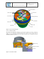
3.3
CRYOSTAT AND MECHANISMS ......................................................................................... 87
3.3.1
3.3.1.1
Cryostat..................................................................................................................... 87
Requirements ..................................................................................................................................... 87
3.3.1.1.1
Temperature................................................................................................................................. 87
3.3.1.1.2
Cooling system ............................................................................................................................ 87
3.3.1.1.3
Flexure......................................................................................................................................... 87
3.3.1.2
Design Report .................................................................................................................................... 87
PANIC
PRELIMINARY DESIGN REPORT
PANIC-GEN-SP-01
0/1
22 October 2007
11 of 183
3.3.1.2.1
Vacuum can ................................................................................................................................. 88
3.3.1.2.2
Nitrogen vessel for cold bench cooling........................................................................................ 88
3.3.1.2.3
Nitrogen vessel for detector cooling ............................................................................................ 89
3.3.1.2.4
Spacers......................................................................................................................................... 89
3.3.1.2.5
Thermal connection of the detector.............................................................................................. 90
3.3.1.2.6
Thermal investigations................................................................................................................. 91
3.3.1.2.6.1
Nitrogen vessel for cold bench ............................................................................................. 91
3.3.1.2.6.2
Nitrogen vessel for detector cooling..................................................................................... 91
3.3.1.2.6.3
Thermal gradient .................................................................................................................. 91
3.3.1.2.7
3.3.2
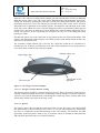
Telescope adapter ........................................................................................................................ 93
Mechanisms............................................................................................................... 94
3.3.2.1
Requirements ..................................................................................................................................... 94
3.3.2.2
Design Report .................................................................................................................................... 94
3.3.2.2.1
Entrance window ......................................................................................................................... 96
3.3.2.2.2
Mounting of cryogenic lenses and mirrors................................................................................... 97
3.3.2.2.3
Optics wheel unit ....................................................................................................................... 100
3.3.2.2.4
Filter wheel unit......................................................................................................................... 103
3.3.2.2.5
Rotating field stop...................................................................................................................... 105
3.3.2.2.6
Detector mount .......................................................................................................................... 106
3.3.2.2.7
FEM simulation results.............................................................................................................. 106
3.3.2.2.7.1
3.4
Code:
Iss/Rv:
Date:
Page:
Simulation of cryostat with optics replaced by point masses.............................................. 106
3.3.2.2.7.1.1
Telescope pointing to zenith ....................................................................................... 107
3.3.2.2.7.1.2
Telescope pointing to horizon ..................................................................................... 109
3.3.2.2.7.2
FEM simulation of a detailed model................................................................................... 110
3.3.2.2.7.3
Bending of entrance window.............................................................................................. 112
3.3.2.2.7.4
Bending of mirror M1 due to gravity.................................................................................. 113
3.3.2.2.8
Error budget............................................................................................................................... 114
3.3.2.2.9
Total weight limit and possible solutions................................................................................... 117
ELECTRONICS ................................................................................................................. 120
3.4.1
ROE......................................................................................................................... 120
3.4.1.1
Scope ............................................................................................................................................... 120
3.4.1.2
Requirements ................................................................................................................................... 120
3.4.1.3
General Information......................................................................................................................... 120
3.4.1.3.1
ROCon – ReadOutController..................................................................................................... 122
3.4.1.3.2
AD36 - 36 channel analog to digital converter .......................................................................... 122
3.4.1.3.3
H2RG_CB - HAWAII2RG Clock/Bias board ........................................................................... 123
3.4.1.3.4
BP6 - 6 slot backplane ............................................................................................................... 124
3.4.1.3.5
OPTPCI - fiberlink interface...................................................................................................... 124
3.4.1.3.6
CA36 – 36 channel cryogenic preamplifier ............................................................................... 125
3.4.1.3.7
Power Supply............................................................................................................................. 125
PANIC
PRELIMINARY DESIGN REPORT
PANIC-GEN-SP-01
0/1
22 October 2007
12 of 183
3.4.1.3.8
Detector protection circuitry ...................................................................................................... 125
3.4.1.3.9
Troubleshooting - Diagnostics................................................................................................... 126
3.4.2
Control Electronics ................................................................................................. 128
3.4.2.1
Requirements ................................................................................................................................... 128
3.4.2.2
General electronics concept ............................................................................................................. 129
3.4.2.2.1
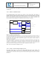
Overview ................................................................................................................................... 129
3.4.2.2.2
Simplified block diagramm of instrument control electronics ................................................... 129
3.4.2.3
Motion control electronics ............................................................................................................... 130
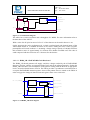
3.4.2.3.1
General ...................................................................................................................................... 130
3.4.2.3.2
Principle of motion control system ............................................................................................ 130
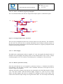
3.4.2.3.3
Motion controller board (MOCON)........................................................................................... 131
3.4.2.3.4
Stepper Motor Driver (SMD8)................................................................................................... 131
3.4.2.4
PANIC motors ................................................................................................................................. 132
3.4.2.4.1
3.4.2.5
General ...................................................................................................................................... 132
Position and reference marks ........................................................................................................... 132
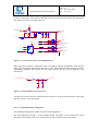
3.4.2.5.1
Microswitches............................................................................................................................ 132
3.4.2.5.2
Resolver ..................................................................................................................................... 133
3.4.2.5.3
Resolver Module (RESMOD).................................................................................................... 133
3.4.2.6
Motion controlled units.................................................................................................................... 134
3.4.2.6.1
Filter unit ................................................................................................................................... 134
3.4.2.6.2
Optics and field stops wheel ...................................................................................................... 134
3.4.2.7
3.5
Code:
Iss/Rv:
Date:
Page:
Resources......................................................................................................................................... 135
3.4.2.7.1
Power consumption and weight ................................................................................................. 135
3.4.2.7.2
Instrumentation rack .................................................................................................................. 135
SOFTWARE ...................................................................................................................... 136
3.5.1
Summary.................................................................................................................. 136
3.5.2
Introduction............................................................................................................. 136
3.5.3
Requirements........................................................................................................... 136
3.5.3.1
Guides to understanding the requirements....................................................................................... 136
3.5.3.1.1
Use of shall/should ................................................................................................................... 136
3.5.3.1.2
Unconfirmed and undefined requirements................................................................................. 136
3.5.3.2
General Requirements ..................................................................................................................... 136
3.5.3.2.1
Parts ........................................................................................................................................... 136
3.5.3.2.2
Operating System....................................................................................................................... 136
3.5.3.2.3
System Log ................................................................................................................................ 137
3.5.3.3
GEIRS ............................................................................................................................................. 137
3.5.3.3.1
Hardware minimum requirements ............................................................................................. 137
3.5.3.3.2
Interfaces ................................................................................................................................... 137
3.5.3.3.2.1
Instrument Status................................................................................................................ 137
3.5.3.3.2.2
Control Electronics............................................................................................................. 138
PANIC
PRELIMINARY DESIGN REPORT
Code:
Iss/Rv:
Date:
Page:
PANIC-GEN-SP-01
0/1
22 October 2007
13 of 183
3.5.3.3.2.3
Readout Electronics (ROE) ................................................................................................ 138
3.5.3.3.2.4
Telescope............................................................................................................................ 139
3.5.3.3.2.5
OT ...................................................................................................................................... 139
3.5.3.3.3
Data............................................................................................................................................ 139
3.5.3.3.4
Filter focus................................................................................................................................. 139
3.5.3.3.5
Guiding ...................................................................................................................................... 140
3.5.3.4
Observation Tool (OT) .................................................................................................................... 140
3.5.3.4.1
Functionality .............................................................................................................................. 140
3.5.3.4.2
Hardware requirements.............................................................................................................. 140
3.5.3.4.3
External Interfaces ..................................................................................................................... 140
3.5.3.4.3.1
Graphical User Interface (GUI) .......................................................................................... 140
3.5.3.4.3.2
Hardware Interfaces............................................................................................................ 140
3.5.3.4.3.3
Software Interfaces............................................................................................................. 140
3.5.3.4.3.3.1
GEIRS Interface.......................................................................................................... 140
3.5.3.4.3.3.2
Telescope Interface ..................................................................................................... 140
3.5.3.4.3.3.3
On-line star catalog ..................................................................................................... 140
3.5.3.4.4
Display....................................................................................................................................... 141
3.5.3.4.5
Observing definition .................................................................................................................. 141
3.5.3.4.6
Calibration definition................................................................................................................. 141
3.5.3.4.7
Survey/Mosaic definitions ......................................................................................................... 141
3.5.3.4.8
Templates................................................................................................................................... 141
3.5.3.4.9
Dome segments shift.................................................................................................................. 142
3.5.3.4.10
Validation ................................................................................................................................ 142
3.5.3.4.11
Execution Control .................................................................................................................... 142
3.5.3.4.12
Output scripts........................................................................................................................... 142
3.5.3.4.13
Extra keywords ........................................................................................................................ 142
3.5.3.4.14
GEIRS Functionalities ............................................................................................................. 142
3.5.3.4.15
Secondary mirror focusing....................................................................................................... 142
3.5.3.4.16
Simulation................................................................................................................................ 143
3.5.3.4.17
Observing Modes..................................................................................................................... 143
3.5.3.4.18
Efficiency................................................................................................................................. 143
3.5.3.4.19
Flexible .................................................................................................................................... 143
3.5.3.4.20
On/Off-line .............................................................................................................................. 143
3.5.3.4.21
Timeline Calculator ................................................................................................................. 143
3.5.3.4.22
Exposure Time Calculator ....................................................................................................... 143
3.5.3.4.23
Engineering support................................................................................................................. 143
3.5.3.4.24
Errors & Warnings................................................................................................................... 143
3.5.3.4.25
Repository................................................................................................................................ 144
3.5.3.5
Quicklook Tool................................................................................................................................ 144
3.5.3.5.1
General requirements................................................................................................................. 144
PANIC
PRELIMINARY DESIGN REPORT
Code:
Iss/Rv:
Date:
Page:
PANIC-GEN-SP-01
0/1
22 October 2007
14 of 183
3.5.3.5.1.1
Quick feedback................................................................................................................... 144
3.5.3.5.1.2
Quality control.................................................................................................................... 144
3.5.3.5.2
Observing Utilities..................................................................................................................... 144
3.5.3.5.2.1
Focus .................................................................................................................................. 144
3.5.3.5.2.2
Seeing................................................................................................................................. 144
3.5.3.5.3
Data reduction tasks................................................................................................................... 144
3.5.3.5.4
Extensions.................................................................................................................................. 144
3.5.3.5.5
Quick data persistence ............................................................................................................... 144
3.5.3.6
Data Reduction Software ................................................................................................................. 144
3.5.3.6.1
Quick pipeline............................................................................................................................ 144
3.5.3.6.1.1
Dark current subtraction ..................................................................................................... 145
3.5.3.6.1.2
Flatfielding ......................................................................................................................... 145
3.5.3.6.1.3
Bad pixel correction ........................................................................................................... 145
3.5.3.6.1.4
Raw sky modeling .............................................................................................................. 145
3.5.3.6.1.5
Shift and align .................................................................................................................... 145
3.5.3.6.1.6
Fast Astrometry .................................................................................................................. 145
3.5.3.6.2
Science pipeline ......................................................................................................................... 145
3.5.3.6.2.1
Master calibration frames ................................................................................................... 145
3.5.3.6.2.2
Dark current substraction.................................................................................................... 145
3.5.3.6.2.3
Flatfielding correction ........................................................................................................ 145
3.5.3.6.2.4
Bad/hot pixel removal ........................................................................................................ 145
3.5.3.6.2.5
Fringe correction ................................................................................................................ 146
3.5.3.6.2.6
Cosmic rays removal .......................................................................................................... 146
3.5.3.6.2.7
Sky modeling...................................................................................................................... 146
3.5.3.6.2.8
Shift and align (Dithering and Stacking) ............................................................................ 146
3.5.3.6.2.9
Gap elimination .................................................................................................................. 146
3.5.3.6.2.10
Scale Modes ..................................................................................................................... 146
3.5.3.6.2.11
Astrometry Requirements................................................................................................. 146
3.5.3.6.2.11.1
Absolute Astrometry ................................................................................................. 146
3.5.3.6.2.11.2
Relative Astrometry .................................................................................................. 146
3.5.3.6.2.11.3
World Coordinate System (WCS) ............................................................................. 146
3.5.3.6.2.12
Photometric Requirements ............................................................................................... 146
3.5.3.6.2.12.1
Absolute Photometric in J, H, Ks .............................................................................. 146
3.5.3.6.2.12.2
Absolute Photometric in Y,z ..................................................................................... 146
3.5.3.6.2.13
Ghosts............................................................................................................................... 147
3.5.3.6.2.14
Field distortion ................................................................................................................. 147
3.5.3.6.2.15
Image stability .................................................................................................................. 147
3.5.3.6.2.16
Catalog generation............................................................................................................ 147
3.5.3.6.3
3.5.3.7
Hardware Requirements ............................................................................................................ 147
Data Collection And Data Rates Requirements ............................................................................... 147
PANIC
PRELIMINARY DESIGN REPORT
Code:
Iss/Rv:
Date:
Page:
PANIC-GEN-SP-01
0/1
22 October 2007
15 of 183
3.5.3.7.1
Data volume............................................................................................................................... 147
3.5.3.7.2
Data storage ............................................................................................................................... 147
3.5.3.7.2.1
Disk .................................................................................................................................... 147
3.5.3.7.2.2
Access ................................................................................................................................ 147
3.5.3.7.3
Delivering format....................................................................................................................... 147
3.5.3.7.3.1
3.5.3.7.4
FITS headers ...................................................................................................................... 147
Saving Modes ............................................................................................................................ 147
3.5.3.7.4.1
Data type size ..................................................................................................................... 148
3.5.3.7.4.2
File structure....................................................................................................................... 148
3.5.3.7.5
Archive and VO......................................................................................................................... 149
3.5.3.7.5.1
Archiving............................................................................................................................ 149
3.5.3.7.5.2
Virtual Observatory ............................................................................................................ 149
3.5.3.7.5.2.1
3.5.3.8
3.5.4
VO data model ............................................................................................................ 149
Caha Sw Requirements.................................................................................................................... 149
Design Report ......................................................................................................... 150
3.5.4.1
Instrument Control Software ........................................................................................................... 150
3.5.4.2
Data Handling Software................................................................................................................... 150
3.5.4.3
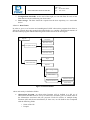
Network Layout............................................................................................................................... 151
3.5.4.4
Computer Architecture .................................................................................................................... 152
3.5.4.5
GEIRS Design description............................................................................................................... 153
3.5.4.5.1
GEIRS integration time and data specifications......................................................................... 154
3.5.4.5.2
Read-out with high speed........................................................................................................... 155
3.5.4.5.3
Read noise reduction.................................................................................................................. 156
3.5.4.5.4
Guiding ...................................................................................................................................... 157
3.5.4.5.5
Parts ........................................................................................................................................... 157
3.5.4.6
Observation Tool description........................................................................................................... 158
3.5.4.6.1
Purpose ...................................................................................................................................... 158
3.5.4.6.2
Observing strategies................................................................................................................... 158
3.5.4.6.3
Data Entities .............................................................................................................................. 159
3.5.4.6.4
Workflow................................................................................................................................... 162
3.5.4.6.5
The Observation Tool Editor ..................................................................................................... 163
3.5.4.6.6
Programming language and components ................................................................................... 164
3.5.4.7
Quicklook description...................................................................................................................... 164
3.5.4.7.1
Purpose ...................................................................................................................................... 164
3.5.4.7.2
Implementation .......................................................................................................................... 164
3.5.4.8
Data reduction software description ................................................................................................ 164
3.5.4.8.1
Purpose ...................................................................................................................................... 164
3.5.4.8.2
Data Flow .................................................................................................................................. 165
3.5.4.8.3
General data reduction schemes................................................................................................. 166
3.5.4.8.3.1
Main steps .......................................................................................................................... 166
PANIC
PRELIMINARY DESIGN REPORT
PANIC-GEN-SP-01
0/1
22 October 2007
16 of 183
3.5.4.8.3.1.1
Detector Calibration:................................................................................................... 167
3.5.4.8.3.1.2
Fringing....................................................................................................................... 167
3.5.4.8.3.1.3
Sky modelling and extraction...................................................................................... 168
3.5.4.8.3.1.4
Shift and align ............................................................................................................. 168
3.5.4.8.3.1.5
Electronic Crosstalk correction ................................................................................... 169
3.5.4.8.3.1.6
Optical ghosts removal................................................................................................ 169
3.5.4.8.3.1.7
Field distortion correction ........................................................................................... 169
3.5.4.8.3.1.8
Mosaicing.................................................................................................................... 169
3.5.4.8.3.1.9
Astrometry and Photometry ........................................................................................ 170
3.5.4.8.3.2
Quick look Mode................................................................................................................ 170
3.5.4.8.3.3
Science Mode ..................................................................................................................... 170
3.5.4.8.4
3.6
Code:
Iss/Rv:
Date:
Page:
Implementation overview .......................................................................................................... 172
MAINTENANCE / OPERATION.......................................................................................... 173
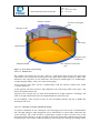
3.6.1
Summary.................................................................................................................. 173
3.6.2
Introduction............................................................................................................. 173
3.6.3
Technical Requirements .......................................................................................... 173
3.6.3.1
Synopsis:.......................................................................................................................................... 173
3.6.3.2
Mechanics:....................................................................................................................................... 173
3.6.3.3
Electronics: ...................................................................................................................................... 174
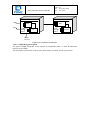
3.6.3.3.1 The electronics Rack can be mounted under the mirror cell, independent of the cryostat. This
means that the cable length between the electronics rack and the cryostat will be about 4m........................ 174
3.6.3.3.2
To guarantee the best technical support CAHA needs a full spare electronics set..................... 174
3.6.3.3.3
Before first light, Calar Alto staff needs a full documentation set (in English). ........................ 174
3.6.3.3.4
Regarding electronics the documentation should include: ......................................................... 174
3.6.3.3.4.1
Block schematics for cabling between different electronic units........................................ 174
3.6.3.3.4.2
Block schematics for each electronic board........................................................................ 174
3.6.3.3.4.3
Detailed schematics for each electronic board.................................................................... 174
3.6.3.3.4.4
Detailed electrical cabling for each electronic subsystem. ................................................. 174
3.6.3.3.4.5
Cabling through the telescope to be decided together with Calar Alto staff....................... 174
3.6.3.3.4.6
Documentation about non standard components. ............................................................... 174
3.6.3.3.4.7
Documentation about test programs and adjusting procedures........................................... 174
3.6.3.3.4.8 Extended users manual with all necessary for trouble shooting including serial and parallel
port configuration. .................................................................................................................................... 174
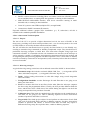
3.6.3.3.5 The maximum acceptable power dissipation under the mirror cell will be 100W. If more is
needed, a cooling system should be implemented......................................................................................... 174
3.6.3.3.6 .Before first light, at least 2 technicians from Calar Alto staff need a complete training about the
electronics and software................................................................................................................................ 174
3.6.3.3.7 For at least the first year Calar Alto needs a contact person to solve the unforeseen problems that
will appear until the system is stable and Calar Alto staff has a complete knowledge of the instrument. This
contact person should be reachable also during vacations and occasionally, but rarely, during the night and
weekends. 174
3.6.3.3.8 The first PANIC observations will be done during instrument commissioning and in contact with
the hardware and software designers (if possible present at Calar Alto)....................................................... 174
PANIC
PRELIMINARY DESIGN REPORT
3.6.3.4
Code:
Iss/Rv:
Date:
Page:
PANIC-GEN-SP-01
0/1
22 October 2007
17 of 183
Software:.......................................................................................................................................... 174
3.6.3.4.1
The disk organization will be as follow: .................................................................................... 174
3.6.3.4.1.1
One disk for the system installation (/boot, swap, and / partitions). ................................... 174
3.6.3.4.1.2
One disk for the whole instrument software (/disk-a)......................................................... 175
3.6.3.4.1.3
One or more disks for data (/disk-b …).............................................................................. 175
3.6.3.4.1.4
Filesystem ext3................................................................................................................... 175
3.6.3.4.2 The system installation will be done by Calar Alto staff according to its own standards, SuSE
Operating system, and Pc based computer.................................................................................................... 175
3.6.3.4.3 Before first light Calar Alto needs a full backup of all necessary software installed in the
computers necessary for the normal operation. This backup system will be tested before first light. CAHA
requirements for PANIC, August 2007......................................................................................................... 175
3.6.3.4.4
Any non standard part in the Pc shout be acquired together with a spare part. .......................... 175
3.6.3.4.5
Regarding software the final documentation should include: .................................................... 175
3.6.3.4.5.1
Disk structure. .................................................................................................................... 175
3.6.3.4.5.2
Directory structure for the software.................................................................................... 175
3.6.3.4.5.3
Start and user scripts........................................................................................................... 175
3.6.3.4.5.4
Test scripts, help programs and debug................................................................................ 175
3.6.3.4.5.5
Description about Log files. ............................................................................................... 175
3.6.3.4.5.6
Changes done in the standard operating system. ................................................................ 175
3.6.3.4.5.7
Normal programs installed in the system............................................................................ 175
3.6.3.4.5.8
Description for the different versions if available. ............................................................. 175
3.6.3.4.5.9
Description about the network structure. ............................................................................ 175
3.6.3.4.5.10
Hardware and software fail procedures (How-to’s).......................................................... 175
3.6.3.4.6
In case it will be needed by CAHA staff, training of software operation will be required......... 175
3.6.3.4.7
It is recommendable to have a RAID system to prevent data losses, as well as a DAT unit...... 175
3.6.3.4.8
If possible the hardware should be acquired in Spain for warranty issues. ................................ 175
3.6.3.5
Optics and cryogenics:..................................................................................................................... 175
3.6.3.5.1 In case that the optical fine adjustments will be done on Calar Alto, it would be desirable to
mount a clean room. This room can later be used for filter changes, and all works to be done on the cryostat.175
3.6.3.5.2 Transmission curves (including red leaks beyond 2.5 μm) for all filters and the other optical
elements should be supplied in paper and electronic (ASCII) format. .......................................................... 175
3.6.3.5.3
CAHA.
3.6.3.6
3.6.4
The drawings of the optics shall be delivered in electronic form in a format agreed upon with
175
Acceptance: ..................................................................................................................................... 176
Operation ................................................................................................................ 176
4.
MANAGEMENT.......................................................................................................... 178
4.1
SUMMARY....................................................................................................................... 178
4.2
WORK PACKAGES ........................................................................................................... 178
4.3
THE PANIC TEAM ............................................................................................................ 179
4.4
ASSEMBLY AND INTEGRATION ....................................................................................... 180
4.5
MANPOWER .................................................................................................................... 180
PANIC
PRELIMINARY DESIGN REPORT
Code:
Iss/Rv:
Date:
Page:
PANIC-GEN-SP-01
0/1
22 October 2007
18 of 183
4.6
COST AND FINANCIAL PLAN ........................................................................................... 181
4.7
SCHEDULE ...................................................................................................................... 182
PANIC
PRELIMINARY DESIGN REPORT
Code:
Iss/Rv:
Date:
Page:
PANIC-GEN-SP-01
0/1
22 October 2007
19 of 183
LIST OF FIGURES
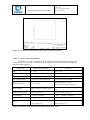
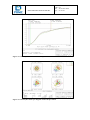
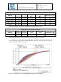
Figure 2-1 Improvement of the photometric precision if a small pixel size (compared to the
seeing) is used. .................................................................................................................... 33
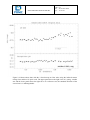
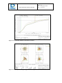
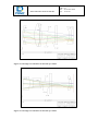
Figure 2-2 Observations done with the 3.5m telescope at Calar Alto, using the infrared camera
Omega Cass and the 0.2"/pixel scale. The upper panel shows the light curve of a young,
variable star and the lower panel shows the light curve of a reference star; the standard
deviation of the second star is 3 millimagnitudes. .............................................................. 34
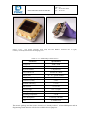
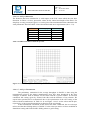
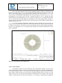
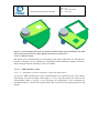
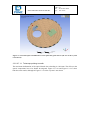
Figure 3.1.6-1. The mosaic assembly plate (left) and four H2RG’s mounted into it (right).
Courtesy of Teledyne Scientific and Imaging, LLC. .......................................................... 38
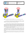
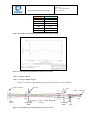
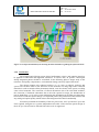
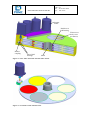
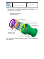
Figure 3.2.6-1 PANIC location in the RC focus of the 2.2 m telescope ..................................... 48
Figure 3.2.6-2 Optics layout of PANIC: left the 0.45”/px camera and right the 0.25”/px camera.
............................................................................................................................................. 49
Figure 3.2.6-3 Optics layout of de PANIC the 0.45”/px camera ................................................ 50
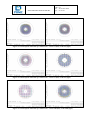
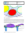
Figure 3.2.6-4 Footprint of the 0.45”/px camera FOV: on the Entrance window (left), on the L0
(right)................................................................................................................................... 52
Figure 3.2.6-5 Footprint of the 0.45”/px camera FOV: on the M1 (left up), on the M2 (right up)
and on the M3 (bottom)....................................................................................................... 53
Figure 3.2.6-6 Footprint of the 0.45”/px camera FOV: on the L1 (left), on the L2 (right)......... 53
Figure 3.2.6-7 Footprint of the 0.45”/px camera FOV: on the L3 (left), on the L4 (right)......... 54
Figure 3.2.6-8 Footprint of the 0.45”/px camera FOV: on the L5A (left), on the L6A (right). .. 54
Figure 3.2.6-9 Footprint of the 0.45”/px camera FOV: on the L7A (left), on the L8A (right). .. 54
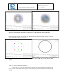
Figure 3.2.6-10 Footprint of the 0.45”/px camera FOV on the detector plane ........................... 55
Figure 3.2.6-11 Complete FOV of the 0.45”/px.......................................................................... 56
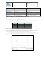
Figure 3.2.6-12 Polychromatic EE of the 0.45”/px camera ........................................................ 58
Figure 3.2.6-13 Polychromatic spot diagram of the 0.45”/px camera......................................... 58
Figure 3.2.6-14 Distortion plot for the 0.45”/px camera............................................................. 59
Figure 3.2.6-15 Expected transmission for the 0.45”/px camera ................................................ 60
Figure 3.2.6-16 Optics layout of de PANIC the 0.25”/px camera .............................................. 60
Figure 3.2.6-17 Footprint of the 0.25”/px camera FOV: on the Entrance window (left), on the
L0 (right). ............................................................................................................................ 62
Figure 3.2.6-18 Footprint of the 0.25”/px camera FOV: on the M1 (left up), on the M2 (right up)
and on the M3 (bottom)....................................................................................................... 62
Figure 3.2.6-19 Footprint of the 0.25”/px camera FOV: : on the L1 (left), on the L2 (right)..... 63
Figure 3.2.6-20 Footprint of the 0.25”/px camera FOV: : on the L3 (left), on the L4 (right)..... 63
Figure 3.2.6-21 Footprint of the 0.25”/px camera FOV: : on the L5B (left), on the L6B (right).
............................................................................................................................................. 63
PANIC
PRELIMINARY DESIGN REPORT
Code:
Iss/Rv:
Date:
Page:
PANIC-GEN-SP-01
0/1
22 October 2007
20 of 183
Figure 3.2.6-22 Footprint of the 0.25”/px camera FOV: on the L61B (left), on the L7B (right).
............................................................................................................................................. 64
Figure 3.2.6-23 Footprint of the 0.25”/px camera FOV: on the L8B (left), on the detector plane
(right)................................................................................................................................... 64
Figure 3.2.6-24 Complete FOV of the 0.25”/px.......................................................................... 65
Figure 3.2.6-25 Polychromatic EE of the 0.25”/px camera ........................................................ 67
Figure 3.2.6-26 Polychromatic spot diagram of the 0.25”/px camera......................................... 67
Figure 3.2.6-27 Distortion plot for the 0.25”/px camera............................................................. 68
Figure 3.2.6-28 Expected transmission for the 0.25”/px camera ................................................ 69
Figure 3.2.6-29 Angle over the filters for the 0.45”/px camera .................................................. 70
Figure 3.2.6-30 Angle over the filters for the 0.25”/px camera .................................................. 70
Figure 3.2.6-31 Pupil mask shape ............................................................................................... 72
Figure 3.2.6-32 Footprint at the Pupil position ........................................................................... 73
Figure 3.2.7-1 Montecarlo overlay of the EE80 for the tolerances in the 0.45”/px .................... 80
Figure 3.2.7-2 Montecarlo overlay of the EE80 for the tolerances in the 0.25”/px .................... 84
Figure 3.2.8-1 Opto-mechanical layout showing the main assemblies regarding the optical
elements............................................................................................................................... 86
Figure 3.3.1-1: PANIC cryostat setup ......................................................................................... 88
Figure 3.3.1-2: Nitrogen vessel for cold plate............................................................................. 89
Figure 3.3.1-3: Cold-warm spacers from the central ring to the optical bench........................... 90
Figure 3.3.1-4: Temperature distribution with half filled vessel (maximum filling), pointing to
horizon................................................................................................................................. 92
Figure 3.3.1-5: Temperature distribution with almost empty vessel, pointing to horizon .......... 92
Figure 3.3.1-6: PANIC telescope adapter. .................................................................................. 93
Figure 3.3.2-1: Section through PANIC (the vacuum window and the detector unit are not
shown). ................................................................................................................................ 95
Figure 3.3.2-2: Cold bench and optics ....................................................................................... 96
Figure 3.3.2-3: Entrance window................................................................................................ 96
Figure 3.3.2-4: Cold optics of OMEGA2000 with spring loaded cryogenic lens mount............ 98
Figure 3.3.2-5: Displacements of lens and retainer ring due to thermal shrinkage during cooling
from room temperature to 77 K. The arrows in axial direction show movements relative to
the lens mount supporting surface. a) All parts at room temperature, b) Lens mount
cooling, lens and ring still much warmer, c) Cold lens mount, lens cooling, retainer ring
still much warmer, d) Cold lens and lens mount, retainer ring cooling ............................. 99
Figure 3.3.2-6: Optics wheel without housing .......................................................................... 101
Figure 3.3.2-7: Section view of optics wheel unit..................................................................... 102
Figure 3.3.2-8: Optics wheel ball bearing (detail view of Figure 3.3.2-7)................................ 102
Figure 3.3.2-9: Detail view of optics wheel and filter unit ....................................................... 103
PANIC
PRELIMINARY DESIGN REPORT
Code:
Iss/Rv:
Date:
Page:
PANIC-GEN-SP-01
0/1
22 October 2007
21 of 183
Figure 3.3.2-10: Filter wheel unit with four filter wheels. ....................................................... 104
Figure 3.3.2-11: Filter wheel with drive unit. ........................................................................... 104
Figure 3.3.2-12: Detail view of filter wheel.............................................................................. 105
Figure 3.3.2-13: Rotating field stop, total view and section. .................................................... 105
Figure 3.3.2-14: Rotating field stop in two positions with the housing upper part hidden (left:
field stop for 0.25 arcsec/pixel in use, right: field stop for 0.45 arcsec/pixel in use)........ 106
Figure 3.3.2-15: Both optics assemblies have been replaced by point masses (the rest of the
cryostat is not shown)........................................................................................................ 107
Figure 3.3.2-16: Displacement of cold bench with the telescope pointing to zenith (gravity
vector in z-direction) ......................................................................................................... 108
Figure 3.3.2-17: Cryostat displacement with the telescope pointing to zenith (gravity vector in zdirection) ........................................................................................................................... 108
Figure 3.3.2-18: Displacement of cold bench with the telescope pointing to horizon (gravity
vector in -y-direction)........................................................................................................ 109
Figure 3.3.2-19: Cryostat displacement with the telescope pointing to horizon (gravity vector in
-y-direction)....................................................................................................................... 109
Figure 3.3.2-20: Displacement of cold bench and optics with the telescope pointing to horizon
(gravity vector in -y-direction).......................................................................................... 110
Figure 3.3.2-21: Displacement of cold bench and optics with the telescope pointing to horizon
(gravity vector in -x-direction).......................................................................................... 111
Figure 3.3.2-22: Displacement of cold bench and optics with the telescope pointing to zenith
(gravity vector in +z-direction) ......................................................................................... 111
Figure 3.3.2-23: Simulation of entrance window deformation due to a differential pressure of 1
bar...................................................................................................................................... 112
Figure 3.3.2-24: Deformation of mirror M1 due to gravity in -z direction. .............................. 113
Figure 3.3.2-25: Optics mount 2 with mechanical decenter adjustment of lens L2 with
micrometer screws (exploded view). ................................................................................ 115
Figure 3.3.2-26: Section of optics mount 2 ............................................................................... 116
Figure 3.3.2-27: Section of the one-pixel scale design (similar to Figure 3.3.2-1)................... 118
Figure 3.3.2-28: Cold bench and optics of the one-pixel scale design (similar to Figure 3.3.2-2)
........................................................................................................................................... 118
Figure 3.4.1-1 new ROE (left) versus old ROE (right) ............................................................. 121
Figure 3.4.1-2 ROCon block diagramm.................................................................................... 122
Figure 3.4.1-3 AD36 block diagram ......................................................................................... 123
Figure 3.4.1-4 H2RG_CB block diagram ................................................................................. 123
Figure 3.4.1-5 OPTPCI block diagram ..................................................................................... 124
Figure 3.4.1-6 single channel of the CA36 board ..................................................................... 125
Figure 3.4.1-7 Protection circuitry on Clock/Bias board .......................................................... 126
Figure 3.4.1-8 preamplifier protection circuit ........................................................................... 126
PANIC
PRELIMINARY DESIGN REPORT
Code:
Iss/Rv:
Date:
Page:
PANIC-GEN-SP-01
0/1
22 October 2007
22 of 183
Figure 3.4.2-1 PANIC Control System Simplified Block Diagram.......................................... 129
Figure 3.4.2-2 Principle of motion control system.................................................................... 130
Figure 3.4.2-5 Vacuum stepper motor VSS .............................................................................. 132
Figure 3.4.2-8 Resolver Type RE-15 ........................................................................................ 133
Figure 3.4.2-9 RESMOD_V2.................................................................................................... 133
Figure 3.4.2-10 Instrumentation rack ........................................................................................ 135
Figure 3.5.4-1 Software architecture......................................................................................... 151
Figure 3.5.4-2 Network layout .................................................................................................. 152
Figure 3.5.4-3 Computer Architecture ...................................................................................... 153
Figure 3.5.4-4 Overview of the PANIC control software tasks, the access to data, the data flow,
the connection to the hardware and to Observation Tool and to the on-line pipeline
reduction software ............................................................................................................. 154
Figure 3.5.4-5 Data Entities ...................................................................................................... 159
Figure 3.5.4-6 OT Workflow .................................................................................................... 163
Figure 3.5.4-7 Browser interface Conceptual Diagram ........................................................... 164
Figure 3.5.4-8 Data flow ........................................................................................................... 166
Figure 3.5.4-9 Quick reduction scheme .................................................................................... 170
Figure 3.5.4-10 Science mode scheme...................................................................................... 171
PANIC
PRELIMINARY DESIGN REPORT
Code:
Iss/Rv:
Date:
Page:
PANIC-GEN-SP-01
0/1
22 October 2007
23 of 183
LIST OF TABLES
Table 3.1.6-1. H2RG Major Characteristics............................................................................... 38
Table 3.2-1 Summary of the PANIC General Specifications ..................................................... 45
Table 3.2-2 Mass estimation for the PANIC optics system ........................................................ 50
Table 3.2-3 Raw mass estimation for the folding mirrors........................................................... 50
Table 3.2-4 Prescriptions data of the common elements of the optical system at its nominal
design temperature .............................................................................................................. 51
Table 3.2-5 Prescriptions data of the elements that only belong to the 0.45”/px scale............... 52
Table 3.2-6 Summary of the PANIC performance in the 0.45”/px scale.................................... 55
Table 3.2-7 Fields used in the 0.45”/px scale.............................................................................. 56
Table 3.2-8 Bandwidths of evaluation of the PANIC optical design and their change in focus for
the 0.45”/px scale ................................................................................................................ 57
Table 3.2-9 EE80 in the 0.45”/px scale....................................................................................... 57
Table 3.2-10 Distortion data in the 0.45”/px scale...................................................................... 59
Table 3.2-11 Values of the expected transmission for the 0.45”/px scale .................................. 60
Table 3.2-12 Prescriptions data of the elements that only belong to the 0.25”/px scale............. 61
Table 3.2-13 Summary of the PANIC performance in the 0.25”/px scale.................................. 65
Table 3.2-14 Fields used in the 0.25”/px scale............................................................................ 65
Table 3.2-15 Bandwidths of evaluation of the PANIC optical design and their change in focus
for the 0.25”/px scale .......................................................................................................... 66
Table 3.2-16 EE80 in the 0.25”/px scale..................................................................................... 66
Table 3.2-17 Distortion data in the 0.25”/px scale...................................................................... 68
Table 3.2-18 Values of the expected transmission for the 0.25”/px scale .................................. 68
Table 3.2-19 Position and size of the Field Stop masks.............................................................. 71
Table 3.2-20 Position and size of the Cold Stop mask................................................................ 72
Table 3.2-21 PANIC ghost analysis for the 0.45”/px scale......................................................... 74
Table 3.2-22 PANIC ghost analysis for the 0.25”/px scale......................................................... 74
Table 3.2-23 PANIC camera groups for the 0.45”/px scale........................................................ 75
Table 3.2-24 PANIC camera groups for the 0.25”/px scale........................................................ 76
Table 3.2-25 Manufacturing tolerances for individual elements for the 0.45”/px scale ............. 77
Table 3.2-26 Integration tolerances within the barrel 1 for the 0.45”/px scale ........................... 78
Table 3.2-27 Integration tolerances within the lens mount 2 for the 0.45”/px scale................... 78
PANIC
PRELIMINARY DESIGN REPORT
Code:
Iss/Rv:
Date:
Page:
PANIC-GEN-SP-01
0/1
22 October 2007
24 of 183
Table 3.2-28 Integration tolerances within the lens mount 3A ................................................... 78
Table 3.2-29 Integration tolerances within the barrel 4A ........................................................... 78
Table 3.2-30 Integration tolerances within the Optics mount 1 .................................................. 79
Table 3.2-31 Integration tolerances within the Optics wheel in the 0.45”/px scale .................... 79
Table 3.2-32 Assembly tolerances for the different units in the 0.45”/px scale ......................... 79
Table 3.2-33 Tolerances for whole instrument to the telescope in the 0.45”/px scale................ 80
Table 3.2-34 Manufacturing tolerances for individual elements for the 0.25”/px scale ............. 81
Table 3.2-35 Integration tolerances within the barrel 1 for the 0.25”/px scale ........................... 82
Table 3.2-36 Integration tolerances within the lens mount 2 for the 0.25”/px scale................... 82
Table 3.2-37 Integration tolerances within the lens mount 3Ba.................................................. 82
Table 3.2-38 Integration tolerances within the lens mount 3Bb ................................................. 82
Table 3.2-39 Integration tolerances within the barrel 4B............................................................ 83
Table 3.2-40 Integration tolerances within the Optics mount 1 for 0.25”/px scale..................... 83
Table 3.2-41 Integration tolerances within the Lens mount 3B .................................................. 83
Table 3.2-42 Integration tolerances within the Optics wheel in the 0.25”/px scale .................... 83
Table 3.2-43 Assembly tolerances for the different units in the 0.25”/px scale ......................... 84
Table 3.2-44 Tolerances for whole instrument to the telescope in the 0.25”/px scale................ 84
Table 3.3-1: Grouping of the optical elements of PANIC for the 0.45 arcsec/pixel scale. ......... 94
Table 3.3-2: Grouping of the optical elements of PANIC for the 0.25 arcsec/pixel scale. ......... 94
Table 3.3-3: Mass estimation of the cryogenic opto-mechanics. ................................................ 95
Table 3.3-4: Material list of cryogenic optical elements and their mounts ................................. 97
Table 3.3-5: Tilts and displacements of optical bench and optical groups. .............................. 110
Table 3.3-6: Overall mass estimation of PANIC with two pixel scales.................................... 117
Table 3.3-7: Overall mass estimation of PANIC with only one pixel scale.............................. 119
Table 3.4.2-1 Summary of electronic devices........................................................................... 129
Table 3.4.2-2 Summary of motion controlled filter wheels ...................................................... 134
Table 3.4.2-3 Summary............................................................................................................. 134
Table 3.4.2-4 Summary of power consumption and weight ..................................................... 135
Table 3.5-1 Expected image rates compared for the subwindow size of 36x36 read pixels asked
for in [AD 2]...................................................................................................................... 156
Table 3.5-2 Table with expected read noise suppression, in case of limitation by read noise
instead of background. ...................................................................................................... 156
Table 3.5-3 Some estimated timings for (multiple) guiding windows embedded between normal
full-frame read-out lines.................................................................................................... 157
PANIC
PRELIMINARY DESIGN REPORT
1.
Code:
Iss/Rv:
Date:
Page:
PANIC-GEN-SP-01
0/1
22 October 2007
25 of 183
PANIC GENERAL
1.1 Introduction
The greatest strength of the Calar Alto observatory is its up-to date instrumentation. Whereas
the 3.5m telescope is well equipped with modern instruments, the 2.2m telescope is lacking
modern instrumentation; an exception is the lucky imager Astralux, but this is a special purpose
instrument for a limited range of applications.
A survey on instrumentation wanted for Calar Alto at MPIA and IAA came independently to the
same result, i.e. a NIR (0.9 to 2.5 microns) imager for the 2.2m telescope. It is obvious that an
instrument with a single 2x2 k detector is not state of the art, so a mosaic of 4 detectors was
envisaged. Science applications would obviously be wide field (>1 square degree) imaging and
surveys, but a collection of ideas at IAA and MPIA showed that there are many very interesting
applications also for single pointed observations. The Calar Alto Instrumentation Committee
recommended to build such an instrument. In October 2006 the project PANIC (Panoramic
Near Infrared Camera for Calar Alto) was started. It is a joint project between IAA and MPIA.
One may argue that an instrument like PANIC should be installed at the 3.5m telescope.
Obviously the 3.5m telescope is more powerful; however, observation time is much more
readily available at the 2.2m telescope, so the disadvantage in light collecting power by a factor
of (2.2/3.5)**2 = 0.4 can be compensated by integration time. Omega 2000 at the 3.5m
telescope is clearly a competing instrument. However, Omega 2000 does not have a cold
entrance pupil and hence has a high thermal background in the K-bands. It is expected that
PANIC, which will have a cold stop, will be more sensitive than Omega2000, and since PANIC
has a four times larger FOV it will be more efficient by factors of a few than Omega2000 in the
K-bands.
PANIC will not be the first instrument of its kind. Competing instruments at telescopes < 4m
are WFCAM at UKIRT, NEWFIRM at Kitt Peak 4m telescope, and WIRCAM at CFHT. In the
southern hemisphere, VISTA (4m telescope) has a 64 Mpixel camera that will cover 2154
square arcmin, its operation shall start mid 2008. It is obvious that because of these competing
instruments the development of PANIC should be fast. However, the proposed science cases for
PANIC show that interesting science can be done with it, even if it is not unique.
PANIC
PRELIMINARY DESIGN REPORT
Code:
Iss/Rv:
Date:
Page:
PANIC-GEN-SP-01
0/1
22 October 2007
26 of 183
1.2 General Requirements
The general requirements that were clear from the start are:
•
•
•
•
Detector size 4096x4096 pixel
Spectral range NIR, i.e. minimum YJHK
Image scale 0.45 arcsec/pixel
2.2m telescope
Additional obvious requirements are
• Instrument must not exceed limits set by the telescope in size and weight
• Flexure of the instrument must not degrade optical quality
• Power dissipation should be kept as low as possible, goal < 200W
• The standard guiding unit on the telescope can not be used since it would vignette the
field of PANIC. So PANIC must have its own guiding system.
1.3 Design Aspects
These requirements have direct consequences on the design of PANIC:
•
•
•
•
•
The optical train is much longer than the maximum allowable length of the instrument
along the optical axis. This requires a folded design. The lateral dimension is not
critical.
The weight limit is a very severe one. According to the original ZEISS documentation,
the weight limit is 300kg at the focus. This has led us not to follow the commonly used
design with two nested tanks, rather our design uses one super-isolated tank with one
small tank to cool the detector. However, both CAFOS and WFI at the twin telescope
on LaSilla exceed this limit without any degradation in telescope performance.
Including the guider unit, CAFOS weighs 400kg and has a torque of 1860Nm. We take
these values as safe limits.
The operating temperature of the detectors is in the range 77-80K, the optimum
temperature has to be found by experiment. From experience with other Rockwell
detectors we expect that the operating temperature should be stable to ± 0.1K.
The cooling system should require as little attention as possible. Since liquid Nitrogen
cooling requires only refilling, we decided to use nitrogen cooling. We are aiming at
holding times longer than 24 hours, although Calar Alto would accept refilling twice a
day.
We try to benefit from experience gained with Omega2000 as much as possible:
PANIC
PRELIMINARY DESIGN REPORT
o
o
o
Code:
Iss/Rv:
Date:
Page:
PANIC-GEN-SP-01
0/1
22 October 2007
27 of 183
Mechanical detail solutions, such as lens holders and filter wheel mechanics,
will be taken over with minimal changes
The read-out electronics is a further development of the older MPIA ROE,
using newer and cheaper ICs. Furthermore the new ROE will read out 132
channels, compared to 36 in Omega2000.
The control electronics will use modules which are standard at MPIA/CAHA
and are in use not only in Omega2000, but also in several other instruments on
Calar Alto. This will reduce not only the time required for development but also
has obvious advantages for documentation, spare parts stock and know-how on
Calar Alto.
1.4 Additional Features
While designing PANIC, several additional features were proposed which go beyond the basic
requirements. The ones we followed up are:
•
Extend the spectral range to 0.82 microns, so PANIC will cover all spectral bands from
the z to K. The z-band has been included for convenience of the observers, in order to
allow z-band observations to complement NIR observations without changing
instrumentation or waiting for another instrument to be mounted. The applications of
PANIC, however, are in the NIR.
•
The use of narrow band (bandwidth = 1% of central wavelength) filters. This requires
that the angle of incidence of the beam does not exceed a certain value. Our optical
design takes this into account.
•
A second pixel scale of 0.25 arcsec/pixel. This image scale will allow higher spatial
resolution and will be very useful under good seeing conditions which prevail
frequently since the median seeing at Calar Alto is 0.89 arcsec in the R band which
corresponds to 0.65 arcsec in the K band. An optics wheel to exchange some parts of
the optics allows to change between the two image scales. A major difficulty imposed
by the optics is the high mechanical precision required in positioning this wheel – 0.45
microns (see mechanics section). However, close to the date of submitting the PDR
documents, it finally turned out that PANIC with 2 image scales well exceeds the
400kg limit. We estimate the difference in mass between a single and two pixel scale
instrument to 80-100 kg. This is so because not only additional hardware is need but
also a larger cryostat with thicker walls, requiring additional Nitrogen because of
increased heat input. We are currently testing the performance of the telescope with
additional weights. A design with only one pixel scale is also presented; this clearly
avoids the weight problem and exceeds the torque only slightly, and the mechanical
tolerances are relaxed.
PANIC
PRELIMINARY DESIGN REPORT
Code:
Iss/Rv:
Date:
Page:
PANIC-GEN-SP-01
0/1
22 October 2007
28 of 183
2. SCIENCE CASES
We list below potential scientific cases that would benefit from the panoramic imaging mode of
this camera. More details for some of them can be found in the Phase A document, section 2. A
(non-exhaustive) compilation of science cases that would benefit from the other TBC observing
modes is also given.
2.1 Extragalactic Astronomy
2.1.1 Extragalactic Surveys
Cosmic evolution in the z range 1.5 – 2.0 can be studied through surveys of specific
areas in the sky in the clean windows of z and J bands, which enormously reduce the
background sky contained in the OH lines originated in the high levels of the
atmosphere, as compared with the corresponding broad band filters. Photometric
redshifts would then be systematically derived in the so called redshift desert.
A wide-field survey covering the SDSS area not contained in the UKIDSS LAS would
provide highly resolved NIR images of the local galaxy population, including studies of
bars, lopsidedness, population gradients and bulge/disk decomposition. Rare objects, as
T+ dwarfs and z ≥ 6 QSOs could be other science goals.
The NIR part of COMBO-17+4 could be completed in 12.5 clear nights.
A deep NIR photometric survey, for sample selection and characterization, would be also
of interest as a previous step for the exploitation of the EMIR NIR multi-object
spectrograph, a common-user instrument for Grantecan.
Characterization of distant galaxies will also benefit from a high-resolution imaging
mode.
2.1.2 GRBs
2.1.2.1 GRBs at high redshift
The detection of GRBs at redshifts beyond z > 7 is currently one the major
astrophysical challenges, due to its deep implications in the reconstruction of the
history of the Universe. However, at redshifts z > 5 the Lyman-α blanketing
prevents the detection of their optical afterglows, so near-IR observations are
required for their identification. The determination of photometric redshifts is
viable with simultaneous multiband observations carried out with medium-class
telescopes like the 2.2m Calar Alto telescope.
2.1.2.2 GRB host galaxies
A dedicated multicolour imaging program running at the 2.2m would allow, for the
first time, to compile a homogeneous large sample of GRB host galaxies and to
apply statistical methods to construct the SED of GRB host galaxies brighter than
R < 24 using photometric points. From the fit of the SED we would infer
information about the following quantities: the photometric redshift, the age of the
dominant stellar population, the extinction AV, the galaxy-type, the favoured IMF,
the total stellar mass of the host galaxy and the host galaxy environment.
PANIC
PRELIMINARY DESIGN REPORT
Code:
Iss/Rv:
Date:
Page:
PANIC-GEN-SP-01
0/1
22 October 2007
29 of 183
2.1.3 Mapping of nearby galaxies
It is well known that at NIR wavelengths the effects of extinction are mitigated, while
galaxy phenomena are hidden at shorter wavelengths. The following studies could be
performed:
2.1.3.1 Morphological characterization
Multiple nuclei, bars, and boxy/peanut-shaped bulges become visible at NIR
wavelengths. The wide field of PANIC is also particularly suitable for mapping the
outer parts of galaxies, where flaring or warping occur. Extremely low surface
brightness halo structures in nearby galaxies could be traced using red giants. A
high-resolution imaging mode will provide access to nuclear parts of galaxies, e.g.
photometric cusps used to measure the mass of the black hole.
2.1.3.2 Star formation and stellar populations
Studying dust-embedded star formation in nearby galaxies. Mapping in [SIII]
0.9069, 0.9532 μm, Paschen & Brackett series, H2, [FeII], CO band head, and their
corresponding continua, would allow to study the excitation mechanisms in regions
of active star formation, as well as detection of the shock effects and possible
impact on the dust attenuation law. They could also be an interesting supplement to
Spitzer data. It will be also possible to detect intermediate age populations in spiral
arms by identifying AGB stars; their stellar photometry is of crucial importance for
understanding and quantifying the importance of the AGB star contribution to the
integral light of (unresolved) stellar populations in distant galaxies. Global
progression of star formation throughout galaxies could be characterized obtaining
accurate maps of the old stellar population mass and comparing them with star
formation measurements.
2.1.3.3 Magnetic field
Polarimetric observations of nearby galaxies allow determining the large scale
distribution of the magnetic field. At a nuclear level information on the geometry
of the narrow and broad band line regions could be inferred. Polarimetric studies of
extragalactic star forming regions will provide information on the dust distribution
as well as on the energizing mechanism of the magnetic field in the thermal
structure of the nebulae.
2.1.4 Distance scale
A measure of the near-IR period-luminosity relation of Cepheids in nearby galaxies as a
function of the metallicity would improve the accuracy of extragalactic distance scales.
2.1.5 Searches for high-redshift quasars
A by product of large area multiband imaging could come the detection of high redshift
(z > 7) quasars, based on the position of the Lyman−α break between the z and K-bands
at z > 7. The high redshift quasar candidates would be subject of specifically planned
spectroscopic observations.
2.1.6 Clusters and Superclusters of galaxies
Broad band observations of clusters and superclusters of galaxies would allow to search
for objects with strong IR excess and/or the selection of candidates to supermassive
starbursts in clusters at intermediate redshift making use of deep narrow band filter
imaging matching their redshifted Hα line.
PANIC
PRELIMINARY DESIGN REPORT
Code:
Iss/Rv:
Date:
Page:
PANIC-GEN-SP-01
0/1
22 October 2007
30 of 183
2.2 Galactic Astronomy
2.2.1 Galactic survey
A proper motion survey is proposed, using 2MASS as the first epoch, over a quarter of
the sky, which will not be covered by any NIR imager. The larger depth of the survey
would allow obtaining a better star/galaxy separation and photometry for all 2MASS
objects and proper motion down to ≈ 10 mas·yr-1.This catalogue would allow searching
for population II very low-mass stars and brown dwarfs. This project is completed by the
case explained in 2.3.4.
2.2.2 Galactic plane and bulge
The wide field of PANIC will allow mapping selected areas of the galactic plane and
bulge. NIR imaging permits a detailed exploration of the large-scale structure of the
Milky Way and the Galactic components in hidden areas of the Milky Way. There are
still controversial or totally unknown parameters in the description of the detailed stellar
structure, e.g. concerning the radial and vertical distribution of the Galactic disc, and its
specific morphology. Halo streams across the galactic plane would be traced using
colour-selected M-stars, as has recently been demonstrated to have spectacular effect by
2MASS.
2.3 Stellar evolution, star formation, exoplanets
2.3.1 Accretion disks of young stars
NIR monitoring of young stars, most of them low mass stars, show variations due mainly
to changes of the innermost parts of the disk. Simultaneous zJHK photometry would
allow studying the variability of the disk (H and K bands, and maybe the J band) at the
same time that the stellar photosphere is monitored in the z band. Hot stellar spots,
thought to induce the changes observed in the inner disk, leave also a fingerprint on the
H and K bands that would be removed before that data are fitted by theoretical models of
the disks. Polarimetric measures can provide in these systems information on the
geometry of the system, since light becomes polarized after dispersion/reflection in
structures like the inner cavities of the disk, etc.
2.3.2 Search for post-AGBs
Post-AGB stars are enshrouded by a dusty CSE which becomes optically thinner at NIR
wavelengths. NIR emission is primarily emitted from the reddened photosphere and from
light scattered by dust grains. Polarimetry would also allow discriminating between the
faint polarised scattered light from the dusty envelope and the bright unpolarized
emission from the central star. This enables the imaging of material that would normally
be lost under the wings of the stellar PSF. It is possible to obtain information on the grain
size distribution, extinction, equator-to-pole ratio density contrast and structure of the
CSE via modelling the observations. This case would benefit from a high-resolution
imaging mode.
2.3.3 Measures of stellar sizes
Lunar occultations in the IR allow to derive very high angular resolution (~1 mas)
information to be used for: close binaries resolution, direct measure of stellar diameters,
resolving objects with extended envelopes (T Tauris, carbon stars, etc). Narrow band
filters will complement broad band ones as they allow a better resolution of diffraction
PANIC
PRELIMINARY DESIGN REPORT
fringes for bright stars.
applications.
Code:
Iss/Rv:
Date:
Page:
PANIC-GEN-SP-01
0/1
22 October 2007
31 of 183
Fast read-out mode should be implemented for these
2.3.4 Low mass objects, exoplanets
The wide field provided by this camera will allow performing efficient searches of faint
brown dwarfs, and, specially, objects with planetary masses, either isolated or far from
their parent star in open clusters.
2.3.4.1 Probing the IMF down to ~ 1-Jupiter mass. A deep star forming region survey.
The closest (not farther than 300 pc) and densest star forming regions will be
surveyed, in order to detect 1-Jupiter mass objects and to extend the IMF of those
regions to that limit. The different regions should also provide a wide range of
initial conditions: stellar density, presence of hot stars, total mass, and/or age. The
long integration times will be split into several epochs, along a few years, in the
way of a photometric monitoring. This variability survey could detect new
eclipsing binaries, transiting planets, stellar variability (rotational periods), etc.
2.3.4.2 Testing the brown dwarf ejection scenario: a survey around Bok globules.
Since in large star forming regions there is a problem in distinguishing the early
brown dwarf halo from mass segregation due to interactions, it is advantageous to
study the distribution of brown dwarfs around more isolated and much less massive
systems containing only a few objects, like Bok globules.
A dozen Bok globules would be observed in three bands: J, H, and Ks, depending
on sensitivity and contaminant rejection potential. Escaping brown dwarfs
detections will be confirmed by spectroscopic and astrometric follow up.
2.3.5 X-ray binary counterparts
Identification of counterparts of X-rays binaries can be performed at NIR wavelengths,
particularly of massive ones, so that high extinction areas towards the galactic disk
and/or centre can be searched. Ellipsoidal variations due to perturbations in the shape of
the donor star can be detected, and multiwavelength photometric data can be modelled to
infer whether the emission is due to the companion star, accretion disc or a possible
relativistic jet. This scientific case would also benefit from a polarimetric mode since the
IR emission from X-ray binaries can be intrinsically polarised because of light scattered
within the system or because there is a significant synchrotron emission at high
frequencies from a compact jet.
2.3.6 Asteroseismology
Phase shifts between different colours increases significantly toward the infrared for nonradial pulsating stars. Time series analysis extended to the NIR increases dramatically
the pulsation modes identification, allowing real asteroseismology of main sequence
stars.
2.3.7 Supernovae searches
The large FOV of PANIC will allow observing large portions of individual clusters of
galaxies, or even whole ones at the same time, boosting the rate of supernova detections.
Once detected, multiband light curves (YJHK) could be constructed, a relevant issue for
the calculation of the total SN luminosity.
PANIC
PRELIMINARY DESIGN REPORT
Code:
Iss/Rv:
Date:
Page:
PANIC-GEN-SP-01
0/1
22 October 2007
32 of 183
2.3.8 Active stars
Photometric time series extended to the NIR constrain the theoretical models of active
stars showing photospheric solar-like activity cycles and give information about
differential rotation and temporal and/or spatial correlations between inhomogeneities at
different atmospheric levels.
2.4 Solar system
2.4.1 Trans-Neptunian’s, minor bodies
A survey to study NIR colors and short-term variability of a good sample of TNOs,
centaurs and other minor planets could be performed with PANIC, together with a search
for very slowly moving objects in the largest possible fraction of the sky, at least ± 30
degrees above the ecliptic. For that goal, the 2MASS archive would be used as the initial
epoch.
2.4.2 Comets
The most visible and distinctive features of comets are the dust coma and tail: the
refractory material reflects the solar radiation at every wavelength from the near-UV to
the sub-mm range. Systematic observations of comets belonging to different families can
be performed in order to follow the comet activity, the dynamical and compositional
evolution of the dust coma and tail, and gas coma as a function of the heliocentric
distance. In the case of the dust, by fitting the observed image with images synthetically
generated by a dust dynamical model, it is possible to put constraints in the distribution
of the dust size and terminal velocity. Making use of cometary images in several
continuum filters, the dust colour can be measured as a function of the projected
cometocentric distance as well as a function of the heliocentric distance. The dust colour,
combined with similar measurement in the optical range, allow constraining the
mineralogical composition of the dust grains. If polarimetry is also provided, most of the
uncertainties arising from the dust colour analyses can be cleared up.
2.5 JUSTIFICATION FOR A SECOND PIXEL SCALE
The need of a smaller pixel scale is given by the fact that the average seeing at Calar
Alto in the V band is 0.9" (S.F. Sanchez, J. Aceituno, U. Thiele, D. Perez-Ramirez, J. Alves,
arXiv:0709.0813, "The night-sky at the Calar Alto Observatory"), that is, 0.67" in the K band.
From Sanchez et al.'s Fig.5 one can compute that 51% of the nights have seeing ≤0.67" in the K
band. During these nights the images will be undersampled. In order to avoid this situation, a
smaller pixel scale has been proposed and the optical design has incorporated it.
PANIC
PRELIMINARY DESIGN REPORT
Code:
Iss/Rv:
Date:
Page:
PANIC-GEN-SP-01
0/1
22 October 2007
33 of 183
Different kind of scientific projects that will profit from a such a pixel scale (0.25"/pixel):
- Morphological studies of extended objects (galaxies, planetary nebulae, etc) .
- Differential photometry with precision of millimagnitudes. Since the light will be spread over
more pixels, differences in their response will be averaged; besides, partial aperture techniques
can be easily applied.
- Detection of faint sources close to bright objects (low mass companions, objects with
planetary masses, etc), because, if the point spread function is oversampled, the saturation level
and saturation effects will be reached only after longer exposure times.
In order to compute the effect of the pixel size on the photometric precision, we have
analyzed a set of 226 K-band images taken with Omega2000 for the Alhambra project (Mariano
Moles et al.) on a certain field. Differential photometry was performed on a bright star of the
field taking as a reference star the weighted average of another 7 stars on the same field. Figure
2-1 shows the brightness difference between the bright star and the reference star for different
values of the seeing, that is, for different ratios of seeing/pixel_size, the pixel size of
Omega2000 being 0.45". The scatter of the data-points decreases as the ratio of the seeing over
the pixel size increases. The larger scatter is obtained for values of this ratio between 1 and 2 (a
seeing below the pixel size cannot be measured, therefore 1 is a lower limit for this ratio). A
pixel size half of the seeing value (or smaller) ensures the best photometric precision. Since a
seeing of ≤0.67" is expected at Calar Alto for 51% of the nights, a pixel size < 0.33" should be
available.
Figure 2-1 Improvement of the photometric precision if a small pixel size (compared to the seeing)
is used.
PANIC
PRELIMINARY DESIGN REPORT
Code:
Iss/Rv:
Date:
Page:
PANIC-GEN-SP-01
0/1
22 October 2007
34 of 183
Figure 2-2 Observations done with the 3.5m telescope at Calar Alto, using the infrared camera
Omega Cass and the 0.2"/pixel scale. The upper panel shows the light curve of a young, variable
star and the lower panel shows the light curve of a reference star; the standard deviation of the
second star is 3 millimagnitudes.
PANIC
PRELIMINARY DESIGN REPORT
Code:
Iss/Rv:
Date:
Page:
PANIC-GEN-SP-01
0/1
22 October 2007
35 of 183
3. REQUIREMENTS AND DESIGN
3.1 Detectors
3.1.1 Summary
PANIC will use a mosaic of four 2k x 2k HAWAII-2RG arrays from Rockwell (now
Teledyne) in order to cover a field of view of approximately 30 arcmin.
3.1.2 Requirements
The following section lists the technical requirements for the PANIC Science Detector
based on the PANIC Scientific Requirements (Ref 01).
3.1.2.1 Number of pixels
The detector shall have a total of 4096 x 4096 pixels.
3.1.2.2 Spectral Range
The detectors should be responsive from 0.82 to 2.42 μm. In the worst case, a minimum
spectral range from 0.95 to 2.42 μm shall be achieved.
3.1.2.3 Guiding
Since the actual autoguider at the Calar Alto 2.2m Telescope vignettes the FOV of PANIC, and
it will have to be removed whenever PANIC is attached to the telescope, the detector shall
support fast readout rates in order to implement a guiding mode using a subframe of the
detector.
3.1.2.4 Flatness
The physical flatness of the detector should be better than ± 40 µm peak to valley from the best
fit plane in order to avoid image degradation.
3.1.3 Introduction
The selection of the science detector was mostly based on cost, availability, and of course
technical requirements. There were 3 options investigated: the 2K x 2K VIRGO detector
from Raytheon, the 4K x 4K new development from Teledyne, and a mosaic of four
HAWAII-2RG detectors also from Teledyne.
The HAWAII-4RG, Teledyne’s new development, was discarded at an early stage of the
project because of cost and risk. The capital cost of the project would have increased in
approximately 0.4 MEuro, and the array was only at a design stage.
On the other hand, the VIRGO detector was more expensive than the HAWAII-2RG, and
since MPIA has gained a lot of experience working with Teledyne detectors, it was
decided to use a mosaic of four 2k x 2k HAWAII-2RG arrays. These arrays were also
preferred because they have a special “guide mode” in which a programmable window
may be read out continuously at high pixel rates for stable tracking of guide stars,
allowing interleaved readout with the full frame science data.
PANIC
PRELIMINARY DESIGN REPORT
Code:
Iss/Rv:
Date:
Page:
PANIC-GEN-SP-01
0/1
22 October 2007
36 of 183
3.1.4 Scope
This document presents the specifications of the NIR-Detectors for PANIC. In addition, the test
procedures for the characterization process and the general handling of the detectors are
described.
3.1.5 Specifications
The following specifications apply under normal operating conditions, and correspond to
the ones given by Teledyne in their offer.
3.1.5.1 Science Detectors
PANIC will use a mosaic of four 2k x 2k HAWAII-2RG, MBE grown HgCdTe, AR coated,
substrate-removed devices from Teledyne.
3.1.5.1.1 Number of pixels
Each detector shall have 2048 x 2048 pixels.
3.1.5.1.2 QE and Spectral Range
The detectors shall be responsive from 0.3 µm to 2.5 µm.
The QE shall be ≥ 75 % in all photometric bands (Y, J, H and K).
3.1.5.1.3 Uniformity of QE
The non-uniformity of QE shall be < 10 % (σ / mean in the QE histogram) in all bands.
3.1.5.1.4 Pixel Pitch
The pixel pitch shall be 18.0 µm, square format.
3.1.5.1.5 Number of Outputs
Each detector shall have 32 outputs that can be operated in parallel in order to reduce
frame times.
3.1.5.1.6 Read Noise
The read noise shall be < 20 e- CDS @ 100 kHz.
3.1.5.1.7 Timing
In subarray mode, an area of 15″x 15″ of the detector shall be read out at a rate of 8
ms/frame, with a goal of 1 ms/frame for fast photometry. This specification was not
given by Teledyne, it was rather defined by the PANIC team based on the scientific
requirements.
3.1.5.1.8 Dark current
The dark current shall be < 0.1 e-/sec at operating temperature.
3.1.5.1.9 Pixel operability
PANIC
PRELIMINARY DESIGN REPORT
Code:
Iss/Rv:
Date:
Page:
PANIC-GEN-SP-01
0/1
22 October 2007
37 of 183
The number of functional pixels shall be ≥ 95%.
3.1.5.1.10 Operating temperature
The operating temperature shall be 77 K ± 5 K.
3.1.5.1.11 Temperature fluctuation
The temperature fluctuation should be less than 0.1 K. This specification was not given
by Teledyne, it was rather defined by the PANIC team.
3.1.5.1.12 Cool down and warm up
The cool down and warm up rates of the detectors shall be < 0.5 K/ min.
3.1.5.1.13 Physical flatness
The surface of each detector shall be flat to ± 40 µm peak to valley.
3.1.5.1.14 Storage temperature limits
The detectors shall be stored safely between 50 K and 310 K.
3.1.5.1.15 Detector identification
Each detector shall be identified by a unique serial number.
3.1.5.2 Mosaic Package
The mosaic package consists of an assembly plate made of molybdenum where the 4 detectors
will be mounted to.
3.1.5.2.1 Flatness
The flatness over the surface of the whole array (4 detectors) shall be ± 40 µm peak to
valley from the best fit plane.
3.1.5.2.2 Dead space
The dead space between the detectors shall be ≤ 3 mm (approx. 167 pix, which
correspond to about 75 arcsec) from one active area edge to the other.
3.1.6 Design
3.1.6.1 Science Detectors
The science detectors are mounted into a molybdenum mosaic assembly plate. This mosaic
integrates four HAWAII-2RG arrays as separate modules into one single thermal and vibration
stable structure allowing precision alignment and physical flatness between all 4 detectors. The
following figure shows a picture of the detectors mounted into the mosaic package, followed by
a table with the major characteristics of these detectors.
PANIC
PRELIMINARY DESIGN REPORT
Code:
Iss/Rv:
Date:
Page:
PANIC-GEN-SP-01
0/1
22 October 2007
38 of 183
Figure 3.1.6-1. The mosaic assembly plate (left) and four H2RG’s mounted into it (right).
Courtesy of Teledyne Scientific and Imaging, LLC.
Table 3.1.6-1. H2RG Major Characteristics
Parameter
Total pixels
Pixel size
Specification
2048 x 2048
18 µm
Physical Flatness
± 40 µm PTV
Pixel readout rate
100 kHz to 5 MHz
Output ports
Charge storage capacity
32 + 2 + “guide window”
> 100000 e-
Read noise (CDS)
≤ 20 e-
Quantum efficiency
≥ 75 %
Dark current
< 0.1 e-/sec
Spectral range
0.3 – 2.5 µm
Pixel operability
≥ 95 %
Operating temperature
≥ 65 K
Power dissipation
Cost
≤ 4 mW @ 100 kHz
$ 350000 each
The mosaic package and the science detectors are already ordered. A Bare Multiplexer and an
Engineering Grade detector will also be available for test purposes.
PANIC
PRELIMINARY DESIGN REPORT
Code:
Iss/Rv:
Date:
Page:
PANIC-GEN-SP-01
0/1
22 October 2007
39 of 183
3.1.6.2 Requirements verification
The following section presents the calculations needed to determine the feasibility of the critical
technical requirements. So far, the most critical requirement regarding the detectors is the
physical flatness of ± 40 µm peak to valley from the best fit plane and its effect on the optical
quality.
Calar Alto 2.2 Telescope:
f 8
Focal ratio:
Plate scale:
11.7″/mm
⇒ 1″ = 85 µm
PANIC Scale:
1″ =
18μm
= 40μm
0.45"
Then, the focal ratio at the detector is:
f 8⋅
40
= f 3.76
85
On the other hand,
tan α =
D 1 1 1
1 1
⋅ = ⋅
= ⋅
= 0.13
2 f 2 f /# 2 3.76
Then,
Δr
α
r
tan α =
Δr
⇒ Δr = 0.13 ⋅ r
r
PANIC
PRELIMINARY DESIGN REPORT
Code:
Iss/Rv:
Date:
Page:
PANIC-GEN-SP-01
0/1
22 October 2007
40 of 183
Now, considering different “r” values:
r
0
10 µm
40 µm
100 µm
Δr
0
1.3 µm
5.3 µm
13 µm
With a physical flatness of ± 40 µm peak to valley from the best fit plane, the blurr will be of
approximately 10 µm.
Considering also the seeing at Calar Alto (0.6″), at 40 µm the blurr is 24 µm. Adding this
values leads to:
Total blurr = 24 2 + 10 2 = 26 μm
Which means that the optical quality is mostly dominated by the seeing, and not by the factor
introduced by the physical flatness of the detectors.
3.1.7 Characterization
The detector characterization will be done at MPIA using the existing cryogenic test
equipment for IR detectors and the real PANIC readout electronics. The final detector
control system PDCS (computer and software) shall be used.
The cryogenic test equipment allows to change detector temperature, insert a filter, and
blank off any light by cold light-tight baffles. This setup has also been used for other
projects using HAWAII-2 detectors e.g. LUCIFER I & II, LINC-NIRVANA,
Omega2000, etc.
Using the real PANIC readout electronics allows a fine tuning of all components in order
to achieve best performance. For cross checks, a spare set of readout electronics will be
available.
3.1.7.1 Tests
The standard parameters of the Omega2000 detector provide a good starting point for
optimization.
3.1.7.1.1 Detector sensitivity and system gain
The system gain relates the output digital numbers (ADU) to the corresponding input
electrons collected at the pixel unit cell. The system gain is expressed in units of
electrons / ADU. With the knowledge of system gain and gain in the signal processing
chain (pre-amp gain), the detector internal conversion gain (in units of µV / electron) can
be determined.
Since system gain (G) and read noise (R) are constant, this leads to a linear correlation
between variance of the signal (N2) and the signal itself (S):
PANIC
Code:
Iss/Rv:
Date:
Page:
PRELIMINARY DESIGN REPORT
PANIC-GEN-SP-01
0/1
22 October 2007
41 of 183
S R2
N = + 2
G G
2
A linear regression fit (y = mx + b) leads to:
m=
1
G
;
b=
R2
G2
The actual MPIA detector readout software GEIRS supports a set of statistical functions
that allow the data calculation from a stack of images for various integration times i.e.
flux levels. Since PANIC detector readout software is based on GEIRS, these statistical
functions will also be available.
3.1.7.1.2 Full well capacity
The full well capacity is estimated from the photon transfer plot (variance versus signal).
The noise increases linearly with the flux signal. Once the signal level approaches the
full well capacity, a noise roll-over is reached due to pixel saturation effects where the
noise no longer obeys Poisson’s statistics.
3.1.7.1.3 Read noise
• Spatial read noise measurement: Two CDS dark frames, each with minimum detector
integration time, are subtracted from each other pixel-by-pixel. The standard deviation
estimated from a defect free region of the resultant frame is divided by √2 and multiplied
by the system gain to get the spatially averaged temporal read noise in electrons rms.
This noise is referred as read noise in a CDS frame.
• Temporal noise: A series of dark frames are obtained with minimum detector
integration time and without any time interval between individual frames. A noise frame
(in ADU) is generated by measuring the noise in every pixel from all the dark frames on
a pixel-by-pixel basis. The resultant noise frame is converted into electrons by
multiplying by the system gain. The result is a histogram of the noise frame in electrons.
The mean of the histogram is the temporal read noise. The standard deviation of the
histogram shows the noise uniformity.
The actual MPIA detector readout software GEIRS supports a set of statistical functions
to perform these tests. Since PANIC detector readout software is based on GEIRS, these
statistical functions will also be available.
3.1.7.1.4 Linearity
The mean and/or median output signal vs. integration time is measured and plotted. The
output signal in ADU is converted into electrons by multiplying it with the system gain.
PANIC
PRELIMINARY DESIGN REPORT
Code:
Iss/Rv:
Date:
Page:
PANIC-GEN-SP-01
0/1
22 October 2007
42 of 183
A least-squares fit to the data from 10% to 80% of the full well gives the linearity
behavior.
3.1.7.1.5 Persistence and cross-talk
Will not be measured at MPIA.
3.1.7.1.6 Quantum efficiency
This test will not be performed. Values will be taken from the manufacturer’s data
sheets.
3.1.7.1.7 Flatness
The flatness of each detector’s surface will be measured by means of a triangulation
method using an xy stage to map the detector area. MPIA owns such an xy stage, and it
will be used to perform the measurements.
3.1.8 Handling, storage and transportation
The main purpose of this section is to describe a series of safe procedures that shall be
followed when handling the science detectors during acceptance, delivery, inspection,
storage, transportation, integration and maintenance.
3.1.8.1 Electrostatic Discharge
Detectors can be damaged by ESD. The science detectors shall be handled only in an ESDprotected area. MPIA counts with integration halls and dedicated labs in which ESD-protected
conditions are fulfilled.
3.1.8.2 Clean room conditions
The detector should be handled under clean room conditions (class 10000). For assembly and
integration, the detector should be handled in a laminar flow area.
3.1.8.3 Detector handling
The handling of the detectors is restricted to well trained persons. Only persons with permission
from MPIA are allowed to handle the detectors.
The handling of the detectors is only allowed with sufficient ESD protection equipment.
The detectors shall not be cleaned. In case cleaning is necessary, contact the responsible person
at MPIA.
Avoid any mechanical shock to the detectors and mosaic package.
PANIC
PRELIMINARY DESIGN REPORT
Code:
Iss/Rv:
Date:
Page:
PANIC-GEN-SP-01
0/1
22 October 2007
43 of 183
3.1.8.4 Storage
The detectors must be stored in their original case under correct environmental conditions.
Temperature: the storage temperature must be between 50 K and 310 K (-220°C and 30°C).
Humidity: the case shall contain humidity absorbent materials.
Only qualified people shall have access to the storage cabinet.
3.1.8.5 Transportation
The detectors must be transported in its original case. The previous rules must also be fulfilled
during transportation.
For transportation across countries, ensure that all custom regulations are fulfilled. Before
shipping the detectors, contact the responsible person at MPIA.
PANIC
PRELIMINARY DESIGN REPORT
Code:
Iss/Rv:
Date:
Page:
PANIC-GEN-SP-01
0/1
22 October 2007
44 of 183
3.2 Optics
3.2.1 Summary
This optics section contains a description of the PANIC Preliminary Optical Design.
The report includes the optics requirements, the optics layout and image quality, a preliminary
ghost analysis and stray light considerations, optical tolerances analysis and a preliminary AIV.
3.2.2 Introduction
PANIC shall be a wide-field infrared imager for the Ritchey-Chrétien (RC) focus of the
Calar Alto (CAHA) 2.2 m telescope.
The camera optical design is a single optical train that images the sky onto the focal
plane at an optical speed of f/3.74, with a plate scale of 0.45 arcsecond per 18 µm pixel. The
detectors are four Hawaii 2RG of 2k x 2k made by Teledyne, mounted in a mosaic giving a field
of view (FOV) of 31.9 arcmin x 31.9 arcmin.
The camera has been provided with a second smaller pixel scale of 0.25 arcsecond per
pixel optimized for a 18 arcmin diameter FOV.
Special care has been taken in the selection of the standard IR materials used for the
optics in order to include the z band and to maximize the instrument throughput. This cryogenic
instrument has been optimized for Y, J, H and K bands.
The mains challenges of this design are: the correction of off-axis aberrations due to the
wide-field available, the correction of chromatic aberration due to the wide spectral coverage,
the introduction of narrow band filters (~1%) in the system minimizing the degradation in the
filter pass-band, and the mechanical constrains in mass and torque at the Ritchey-Chrétien focus
of the telescope.
The optical design produces an internal pupil available for a Lyot stop at the telescope
image pupil placed at the primary mirror.
3.2.3 Scope
The Preliminary Optical Design is described in this optics section..
3.2.4 Simulations
The PANIC optical design has been developed using ZEMAX-EE (Version January
2007). The model includes the optical components of the 2.2 m telescope.
The optical surfaces are defined with respect to the optical axis, which is always parallel to the
Z axis of the local frame of reference by the optical design program. The distance between
optical surfaces is measured along the optical axis and it is defined by a thickness parameter.
3.2.5 OPTICS Requirements
This section summarizes the Requirements established/imposed by the science goals
and the Technical Requirements that derivate of the operational conditions and design choices.
A separate document describes the Science Requirements (RD1) for PANIC.
PANIC
PRELIMINARY DESIGN REPORT
Code:
Iss/Rv:
Date:
Page:
PANIC-GEN-SP-01
0/1
22 October 2007
45 of 183
The Table 3.2-1 summarizes the General Specifications for PANIC.
Focal Station
Cassegrain 2.2 m
FOV
30’ x 30’ for 0.45”/px
Pixel scales
0.45 arcsec/pixel
0.25 arcsec/pixel
Direct Imaging
Over the whole FOV
Pupil image available
Cold stop
Wavelength range
0.95– 2.45 μm with IQ
0.82-0.95 μm able to transmit
IR Detector
4Kx4K
Gap between detectors
Minimum
Operating temperature
80 K
Filters
System focusing mechanism
Broad band: ¿z?YJHK
Narrow band ∼1%
Telescope S2
Table 3.2-1 Summary of the PANIC General Specifications
The optical system is a monobeam design all refractive, being the only mirrors of the
system the ones used for folding and packaging. The design has not been required to have an
internal collimated beam.
3.2.5.1 GENERAL REQUIREMENTS
3.2.5.1.1 Pixel scale
Parent requirement: 4.1.1. in RD1
The optimum scale shall be 0.45″/pixel.
3.2.5.1.2 Wavelength range
Parent requirement: 4.1.2. in RD1
PANIC shall work in the wavelength range 0.95 -2.42 μm and should work in the range
0.82 – 2.42 μm.
3.2.5.1.3 Image quality
Parent requirement: 4.1.3. in RD1
The image quality shall be such that an 80% of the energy is ensquared (EE) in a 0.9” (2
pixels) over the full FOV for each of the broad bands.
PANIC
PRELIMINARY DESIGN REPORT
Code:
Iss/Rv:
Date:
Page:
PANIC-GEN-SP-01
0/1
22 October 2007
46 of 183
3.2.5.1.4 FOV
Parent requirements: 4.1.1. and 5.4.1. in RD1
PANIC when observing with the 0.45”/px scale shall have a FOV of at least 30 arcmin x
30 arcmin.
3.2.5.1.5 Pupil re-imaging quality
Parent requirement: 4.1.4. in RD1
A separate Technical Note (ORD2) describes in details the signal to noise study for
PANIC and imposes the following requirements in the pupil quality:
3.2.5.1.5.1 System pupil
The PANIC pupil has to be placed at the telescope primary mirror (S1).
3.2.5.1.5.2 Accessible pupil image
The Optical design shall provide an accessible pupil image so that a suitable cold mask
shall be used to minimize stray thermal radiation.
3.2.5.1.5.3 Pupil shape and dimension
The maximum degradation in the pupil re-imaging diameter shall be 3% which is less
than a 10% loss in flux for K band.
The central obstruction of the S2 image at the re-imaging pupil plane shall be avoid.
It is not necessary to avoid the structure of the S2 spiders.
3.2.5.1.6 Stray light and Ghosts
Parent requirements: 4.1.5.1 and 4.1.5.2. in RD1
3.2.5.1.6.1 Image/Ghost ratio
The intensity ratio between a ghost image and its source shall be lower than 1e-4 (this
means that for a point source at the detector and at the limit of saturation there shall not
be a single ghost structure contributing more than 6 counts).
3.2.5.1.6.2 Individual Ghost diameter
The diameter of any individual ghost shall be larger than 10” in case the requirement of
Image/Ghost ratio is not fulfilled.
3.2.5.1.6.3 Stray light
The total stray light shall be minimized.
3.2.5.1.7 Band passes
Parent requirements: 4.1.6.1., 4.1.6.2 and 4.1.6.3.in RD1
PANIC shall be designed to allow use of broad and narrow band filters.
PANIC
PRELIMINARY DESIGN REPORT
Code:
Iss/Rv:
Date:
Page:
PANIC-GEN-SP-01
0/1
22 October 2007
47 of 183
3.2.5.1.7.1 Broad band filters
Filters shall be provided for Y, J, H and K bands. A z filter should also be provided if the
0.82 – 2.42 μm range is achieved.
3.2.5.1.7.2 Tolerance for narrow band filters
Parent requirement: 4.1.6.3. in RD1
Since the narrow band filters have widths, on average, of 1% of the central wavelength
of the filter, the maximum shift allowed for this central wavelength shall be 0.3%.
3.2.5.1.8 Field distortion requirement
Parent requirement: 4.1.8. in RD1
Field distortion shall be less than 1.5 % from the field centre.
3.2.5.1.9 Transmission
Parent requirements: 4.1.6.1., 4.1.6.2 and 4.1.6.3.in RD1
There is no number requirement defined for the transmission of PANIC. There is only
the goal to be as high as possible, to optimize the materials to maximize transmission in
the 0.95-2.45 μm range and to work in the z band (from 0.82 μm).
3.2.5.1.10 Environmental conditions
Parent requirement: 5.3. in RD1
PANIC shall be designed to operate and have optical quality under cryogenic conditions
(temperature 80 K and vacuum).
3.2.5.1.11 High-resolution mode
Parent requirements: 4.3. in RD1
Requirements 3.2.5.1.2., 3.2.5.1.5, 3.2.5.1.6, 3.2.5.1.7, 3.2.5.1.8, 3.2.5.1.9 and 3.2.5.1.10
apply to this mode.
3.2.5.1.11.1 Pixel scale
A second pixel scale of 0.25″/pixel shall be implemented in PANIC.
3.2.5.1.11.2 FOV
PANIC when observing with the 0.25”/px scale shall have a FOV of at least a circle with
a diameter of 8 arcmin. The goal is a FOV with a diameter of the circle inscribed in the
detector dimension which is a diameter of 17.76 arcmin.
3.2.5.1.11.3 Image quality
The image quality shall be such that an 80% of the energy is ensquared (EE) in a 0.75”
(3 pixels) over the full FOV for each of the broad bands.
PANIC
PRELIMINARY DESIGN REPORT
Code:
Iss/Rv:
Date:
Page:
PANIC-GEN-SP-01
0/1
22 October 2007
48 of 183
3.2.6 Optics Layout
3.2.6.1 PANIC General Optics layout
Figure 3.2.6-1 shows the location of PANIC in the telescope.
Figure 3.2.6-1 PANIC location in the RC focus of the 2.2 m telescope
Figure 3.2.6-2 shows the optics model solution for the two scales of PANIC.
PANIC
PRELIMINARY DESIGN REPORT
Code:
Iss/Rv:
Date:
Page:
PANIC-GEN-SP-01
0/1
22 October 2007
49 of 183
Figure 3.2.6-2 Optics layout of PANIC: left the 0.45”/px camera and right the 0.25”/px camera.
The PANIC optics design presented in this document has been modelled at cryogenic
temperatures and vacuum. A separate Technical Note (ORD4) describes in details the models
considered to obtain the glass catalogue at 80 K produced for PANIC.
The camera consists of two separate lens systems which will be alternatively inserted
after the cold stop mask, keeping the total distance between the cold stop and the detector fixed
and equal to 437.30 mm. A deep study has been made to evaluate the best solution for the
implementation of that second pixel scale in PANIC and a separate Technical Note (ORD3)
describes in details this second pixel scale study. Finally we decided to implement the classical
solution which consist in a optics wheel that interchanges all the optics elements after the cold
stop as it is shown in the next pages in this document.
The straight layout shown in the Figure 3.2.6-3 and Figure 3.2.6-16 shows a long
instrument (≈1925 mm). Due to the mechanical constrains in length and weight it has been
searched alternatives to make the system more compact and finally the packaging solution
adopted, shown in the Figure 3.2.6-2, introduces three folding flat mirrors in the optical path
between L0 and L1. From the optical performance point of view this packaging proposed has
not effect.
The distances between mirrors have been fixed as shows the Table 3.2-4, which is an optimum
mirror separation, with no possible interference and vignetting and optimizes the cold volume of
the system.
PANIC
PRELIMINARY DESIGN REPORT
Code:
Iss/Rv:
Date:
Page:
PANIC-GEN-SP-01
0/1
22 October 2007
50 of 183
In Table 3.2-2 it is shown the mass estimation for the lenses of PANIC calculated from
the Zemax model. In the calculations are included the cryostat window and the lenses of the two
pixel scales.
Element
Weight (Kg)
Window
2.93
L0 to L4
7.51
L5A to L8A
2.96
L5B to L8B
2.84
Total
16.24
Table 3.2-2 Mass estimation for the PANIC optics system
A raw estimation for the folding mirrors mass, shown in Table 3.2-3, could be made
assuming circular mirrors with a clear aperture diameter and a thickness of the 10% of its
diameter. Notice that this is only a first estimation and the final mirrors could be elliptical shape
(see Figure 3.2.6-5) and with the minimum thickness needed to assure not degradation in the
optical quality. That thickness will be determined for a FEA, taking into account also the holder
design for that element. So the final mirrors weight surely will be less of this estimation.
Element
Weight (Kg)
M1
4.46
M2
3.64
M3
2.37
Total
10.47
Table 3.2-3 Raw mass estimation for the folding mirrors
3.2.6.2 0.45”/px camera
3.2.6.2.1 0.45”/px Optics Layout
Figure 3.2.6-3 shows the unfolded optics layout of the 0.45”/px scale of PANIC.
Telescope flange
RC focus
Pupil
L2
L0
Dewar
window
M1
Field Stop
mask
M2
L1
Filters
L4
L5A
L3
M3
3 Mirrors
Figure 3.2.6-3 Optics layout of de PANIC the 0.45”/px camera
Cold Stop
mask
L6A
Detector
L8A
L7A
PANIC
PRELIMINARY DESIGN REPORT
Code:
Iss/Rv:
Date:
Page:
PANIC-GEN-SP-01
0/1
22 October 2007
51 of 183
3.2.6.2.2 0.45”/px optical prescriptions
The prescription of the system is listed in Table 3.2-4 and Table 3.2-5. In Table 3.2-4
are listed all the common elements of the two pixel scales and in Table 3.2-5 here are listed the
elements of the scale 0.45”/px that only belong to that pixel scale. The nominal length from the
external part of the window to the detector is 1925.36 mm for both scales.
The curvature radius and thicknesses of the lenses are given at 80 K, working temperature of
PANIC. For manufacturing and assembly, those parameters have to be replaced by warm
parameters, using thermal expansion coefficients defined in ORD4.
Element
Curvature radius
(mm) at 80 K
Telescope flange
Plane
54.6
Cryostat window
Plane
Plane
20.0
IR Fused Silica
291.2
411.8
Vacuum
-
33.6
IR Fused Silica
247.0
25.0
Vacuum
145.0
Vacuum
Zerodur® or BK7
(TBD)
L0
424.9674
Plane
Focal plane
M1
Plane
Thickness or Separation
(mm) at 80 K
28.0 (TBD)
255.0
M2
Plane
25.0 (TBD)
275.0
M3
L1
L2
L3
L4
Plane
480.3027
-281.1478
-251.2363
-431.1047
144.1806
121.4225
217.8809
-6469.551
22.0 (TBD)
Material
Aperture ∅ (mm)
296.6
276.3
Vacuum
Zerodur® or BK7
(TBD)
248.7
Vacuum
Zerodur® or BK7
(TBD)
125.0
Vacuum
22.8
CaF2
17.1
Vacuum
8.0
E-SF03
1.0
Vacuum
40.0
IR Fused Silica
46.8
Vacuum
39.8
BaF2
219.0
162.4
152.8
146.1
116.5
Table 3.2-4 Prescriptions data of the common elements of the optical system at its nominal design
temperature
PANIC
PRELIMINARY DESIGN REPORT
Element
Curvature radius
(mm) at 80 K
Thickness or Separation
(mm) at 80 K
148.2
L5A
L6A
L7A
L8A
Detector
246.6815
121.6698
163.4817
-212.7252
-229.7703
-356.7755
-124.6153
283.5234
Code:
Iss/Rv:
Date:
Page:
PANIC-GEN-SP-01
0/1
22 October 2007
52 of 183
Material
Aperture ∅ (mm)
Vacuum
8.0
IR Fused Silica
64.7
Vacuum
34.0
S-FPL51
1.0
Vacuum
8.0
E-SF03
168.1
Vacuum
14.6
S-FTM16
13.0
Vacuum
118.4
146.0
144.6
105.2
FLAT
Table 3.2-5 Prescriptions data of the elements that only belong to the 0.45”/px scale
3.2.6.2.3 0.45”/px descriptions
In this section we present all the footprint for the optical components in the 0.45”/px scale
configuration from Figure 3.2.6-4 to Figure 3.2.6-10.
Figure 3.2.6-4 Footprint of the 0.45”/px camera FOV: on the Entrance window (left), on the L0
(right).
PANIC
PRELIMINARY DESIGN REPORT
Code:
Iss/Rv:
Date:
Page:
PANIC-GEN-SP-01
0/1
22 October 2007
53 of 183
Figure 3.2.6-5 Footprint of the 0.45”/px camera FOV: on the M1 (left up), on the M2 (right up) and
on the M3 (bottom).
Figure 3.2.6-6 Footprint of the 0.45”/px camera FOV: on the L1 (left), on the L2 (right).
PANIC
PRELIMINARY DESIGN REPORT
Code:
Iss/Rv:
Date:
Page:
PANIC-GEN-SP-01
0/1
22 October 2007
54 of 183
Figure 3.2.6-7 Footprint of the 0.45”/px camera FOV: on the L3 (left), on the L4 (right).
Figure 3.2.6-8 Footprint of the 0.45”/px camera FOV: on the L5A (left), on the L6A (right).
Figure 3.2.6-9 Footprint of the 0.45”/px camera FOV: on the L7A (left), on the L8A (right).
PANIC
PRELIMINARY DESIGN REPORT
Code:
Iss/Rv:
Date:
Page:
PANIC-GEN-SP-01
0/1
22 October 2007
55 of 183
Figure 3.2.6-10 Footprint of the 0.45”/px camera FOV on the detector plane
3.2.6.2.4 0.45”/px optical performance
The Table 3.2-6 lists a summary of the characteristics that describe the performance of
PANIC in the 0.45”/px scale. In this table are the figures of merit that provides a rough idea
about the design quality.
Parameter
Requirement (or Goal)
Achieved
FOV
30’ x 30’
31.9’ x 31.9’
Scale at detector
0.45 ”/px
0.45 ”/px
Pupil image
Cold stop available
Mechanical available
Pupil image quality
< 10% loss in flux for K band
< 2% loss in flux all bands
Wavelength range
0.95 – 2.5 μm
Image Quality
EE80 ≤ 2 pixels (36 μm = 0.90")
EE80= 29.8 μm = 0.75" = 1.7 pix.,
max.
Distortion, maximum
< 1.50 % (corner)
< 1.32 % max. (corner)
Transmission
As much as possible
∼ 45%
Gap between detectors
Minimum
167 pixels (minimum)
Broad band: YJHK
Broad band: zYJHK
Narrow band ∼1%
Narrow band ∼1%
Filters
Optimized: 0.95 – 2.5 μm
Good transmission from 0.8 μm
Table 3.2-6 Summary of the PANIC performance in the 0.45”/px scale
(window+9 lenses)
PANIC
PRELIMINARY DESIGN REPORT
Code:
Iss/Rv:
Date:
Page:
PANIC-GEN-SP-01
0/1
22 October 2007
56 of 183
3.2.6.2.5 0.45”/px Ensquared Energy and Spot diagrams
The FOV has been sampled from the centre to the external field in a radial configuration
following the equal area rule. The system has been optimized for the following fields, see Table
3.2-7, to cover the complete detector surface:
Field
X, Y coordinate (º)
X, Y coordinate (mm)
1
(0;0)
(0;0)
2
(0.154, 0.154)
(22.18,22.18)
3
(0.218, 0.218)
(31.39,31.39)
4
(0.266, 0.266)
(38.30,38.30)
Table 3.2-7 Fields used in the 0.45”/px scale
The origin of coordinates is the centre of the detector mosaic. The second column is the fields
on the sky, and the third column is the coordinates at the detector plane.
At the detector plane, the image spots analyzed are located in the coloured points that
shows the Figure 3.2.6-11. The box indicates the total size of the whole detector (including gap
of 167 pixels between detectors).
Figure 3.2.6-11 Complete FOV of the 0.45”/px
The performance of the design is evaluated at the wavelength and bandwidths shown in
Table 3.2-8. Notice that the design has been optimized to this bands except the z band. The
requirement for z band is not optical quality, it is only for transmission in this band. Instead of
PANIC
PRELIMINARY DESIGN REPORT
Code:
Iss/Rv:
Date:
Page:
PANIC-GEN-SP-01
0/1
22 October 2007
57 of 183
this, it can be seen that there is optical quality in z band, so the system is able to work in this
photometric band.
As the filters will be placed in convergent beam, it has been decided to simulate them
by inserting a plate of IR fused silica with a thickness of 12.5 mm between the L7A and L8A. It
is possible to refocus the system by a movement of the telescope S2 along the optical axis, so
the measurements in defocus are referred to the displacement of the S2 from the nominal
position in the polychromatic configuration, and gives the sense ( - forward, i. e. sense toward
the entrance window, + backward, opposite).
Filter
Wavelength (μm)
EFL (mm)
Focus (mm)
Polychromatic
0.95-2.42
8265.17
0.00
z
0.82-0.99
8257.76
+0.029
Y
0.99-1.08
8259.34
-0.014
J
1.08-1.34
8260.20
-0.025
H
1.50-1.80
8262.49
+0.00
K
1.97-2.42
8265.44
+0.011
Table 3.2-8 Bandwidths of evaluation of the PANIC optical design and their change in focus for the
0.45”/px scale
The image quality of the instrument is specified in terms of the 80 % EE (EE80) for
each photometric band, where EE80 is expressed as the square side length which contains the
80% of the image energy. This EE80 is evaluated in Table 3.2-9 using the greater value
obtained in the FOV analyzed.
Note that all the bands are in requirements (EE80 ≤ 2 pixels=36μm=0.90").
Filter
EE80 (μm)
EE80 (pix)
EE80 (arcsec)
z
25.00
1.39
0.63
Y
21.52
1.20
0.54
J
20.86
1.16
0.52
H
26.14
1.45
0.65
K
33.58
1.87
0.84
Polychromatic
29.84
1.66
0.75
Table 3.2-9 EE80 in the 0.45”/px scale
For simplicity, it has been presented only the polychromatic EE in Figure 3.2.6-12, the
X axis is the half side length square of EE and the Y axis represents the fraction of energy
enclosed, where there is indicated with an horizontal line the 80%. In dark it is shown the
diffraction limit of the system.
For simplicity, as well, it has been presented only the polychromatic spot diagram in
Figure 3.2.6-13. This figures shows the geometrical structure of the image at all points of the
field for all the wavelengths considered. Of course, better figures are obtained when the system
is refocusing in the photometric bands. The squared boxes indicate the dimension of two pixels
in the focal plane (36 μm), and the Airy disk for this configuration is indicated with the dark
circle.
PANIC
PRELIMINARY DESIGN REPORT
Code:
Iss/Rv:
Date:
Page:
Figure 3.2.6-12 Polychromatic EE of the 0.45”/px camera
Figure 3.2.6-13 Polychromatic spot diagram of the 0.45”/px camera
PANIC-GEN-SP-01
0/1
22 October 2007
58 of 183
PANIC
PRELIMINARY DESIGN REPORT
Code:
Iss/Rv:
Date:
Page:
PANIC-GEN-SP-01
0/1
22 October 2007
59 of 183
3.2.6.2.6 0.45”/px Distortion
The distortion has been calculated in % with respect to the FOV centre which does not have
distortion. In Table 3.2-10 we present the values for the central wavelength of the filters. For
simplicity we only present in Figure 3.2.6-14 the plot of the maximum distortion obtained in the
work photometric band of PANIC. Notice that all the bands are in requirements (D ≤ 1.5 %).
Filter
z
Y
J
H
K
Wavelength (μm)
0.82-0.99
0.99-1.08
1.08-1.34
1.50-1.80
1.97-2.42
Distortion (%)
1.32
1.31
1.31
1.30
1.29
Table 3.2-10 Distortion data in the 0.45”/px scale
Figure 3.2.6-14 Distortion plot for the 0.45”/px camera
3.2.6.2.7 0.45”/px Transmission
The preliminary estimation for the average throughput in PANIC is done using the
transmittances given by the glasses manufacturers (they have been introduced in the glass
catalogue of PANIC used in Zemax) for the lenses and the cryostat window. It has been
considered AR coating (given by Zemax) both sides and the thickness of any element. We
expect better performance in transmission due to the optimization of the AR coating of the
lenses with the manufacturers. In Table 3.2-11 and Figure 3.2.6-15 are the values and the plot,
respectively, of the expected transmission as function of the wavelength.
In the transmission calculation all the mirrors has been considered, the two telescope
mirrors and the three folding mirrors of PANIC. For the telescope mirrors we have modelled an
aluminium coating and for the PANIC folding mirrors a gold coating.
PANIC
PRELIMINARY DESIGN REPORT
Code:
Iss/Rv:
Date:
Page:
λ (μm)
Transmission (%)
0.95
37.7
1.26
52.9
1.57
53.3
1.88
48.5
2.19
41.2
2.5
41.2
PANIC-GEN-SP-01
0/1
22 October 2007
60 of 183
Table 3.2-11 Values of the expected transmission for the 0.45”/px scale
Figure 3.2.6-15 Expected transmission for the 0.45”/px camera
3.2.6.3 0.25”/px camera
3.2.6.3.1 0.25”/px Optics Layout
Figure 3.2.6-16 shows the unfolded optics layout of the 0.25”/px scale of PANIC.
Telescope flange
RC focus
Pupil
L2
L0
Dewar
window
M1
Field Stop
mask
M2
M3
3 Mirrors
Figure 3.2.6-16 Optics layout of de PANIC the 0.25”/px camera
L1
Filters
L4
L3
L7B
L5B
Cold Stop
mask
L6B
L61B
Detector
L8B
PANIC
PRELIMINARY DESIGN REPORT
Code:
Iss/Rv:
Date:
Page:
PANIC-GEN-SP-01
0/1
22 October 2007
61 of 183
3.2.6.3.2 0.25”/px optical prescriptions
The prescription of the system is listed in Table 3.2-4 and Table 3.2-12. In Table 3.2-4
are listed all the common elements of the two pixel scales and in Table 3.2-12 there are listed
the elements of the scale 0.25”/px that only belong to that pixel scale.
The curvature radius and thicknesses of the lenses are given at 80 K, working temperature of
PANIC. For manufacturing and assembly, those parameters have to be replaced by warm
parameters, using thermal expansion coefficients defined in ORD4.
Element
L5B
L6B
L61B
L7B
L8B
Detector
Curvature radius
(mm) at 80 K
139.967
-271.923
-195.6231
-180.2618
-248.5058
-343.7706
-173.621
57.76894
-160.495
-90.66532
Thickness or Separation
(mm) at 80 K
Material
107.8
Vacuum
39.1
BaF2
2.6
Vacuum
8.0
IR Fused Silica
8.8
Vacuum
37.5
E-SF03
20.1
Vacuum
40.0
BaF2
168.1
Vacuum
14.6
IR Fused Silica
13.0
Vacuum
Aperture ∅ (mm)
91.3
83.1
75.5
60.7
81.0
FLAT
Table 3.2-12 Prescriptions data of the elements that only belong to the 0.25”/px scale
3.2.6.3.3 0.25”/px descriptions
In this section we present all the footprint for the optical components in the 0.25”/px scale
configuration from Figure 3.2.6-17 to Figure 3.2.6-23.
PANIC
PRELIMINARY DESIGN REPORT
Code:
Iss/Rv:
Date:
Page:
PANIC-GEN-SP-01
0/1
22 October 2007
62 of 183
Figure 3.2.6-17 Footprint of the 0.25”/px camera FOV: on the Entrance window (left), on the L0
(right).
Figure 3.2.6-18 Footprint of the 0.25”/px camera FOV: on the M1 (left up), on the M2 (right up)
and on the M3 (bottom).
PANIC
PRELIMINARY DESIGN REPORT
Code:
Iss/Rv:
Date:
Page:
PANIC-GEN-SP-01
0/1
22 October 2007
63 of 183
Figure 3.2.6-19 Footprint of the 0.25”/px camera FOV: : on the L1 (left), on the L2 (right).
Figure 3.2.6-20 Footprint of the 0.25”/px camera FOV: : on the L3 (left), on the L4 (right).
Figure 3.2.6-21 Footprint of the 0.25”/px camera FOV: : on the L5B (left), on the L6B (right).
PANIC
PRELIMINARY DESIGN REPORT
Code:
Iss/Rv:
Date:
Page:
PANIC-GEN-SP-01
0/1
22 October 2007
64 of 183
Figure 3.2.6-22 Footprint of the 0.25”/px camera FOV: on the L61B (left), on the L7B (right).
On the detector plane is box indicates the dimension of the detector mosaic and the circle the
FOV optimized for the 0.25”/px scale.
Figure 3.2.6-23 Footprint of the 0.25”/px camera FOV: on the L8B (left), on the detector plane
(right).
3.2.6.3.4 0.25”/px optical performance
The Table 3.2-13 lists the characteristics that describe the performance of PANIC in the
0.25”/px scale. In this table are the figures of merit that provides a rough idea about the design
quality.
PANIC
PRELIMINARY DESIGN REPORT
Parameter
Code:
Iss/Rv:
Date:
Page:
PANIC-GEN-SP-01
0/1
22 October 2007
65 of 183
Requirement (or Goal)
Achieved
FOV
8’ (or 17.76’) diameter
18.32’ diameter
Scale at detector
0.25 ”/px
0.25 ”/px
Image Quality
EE80 ≤ 3 pixels (54 μm = 0.75")
EE80= 41.4 μm = 0.58" = 2.3 pix.,max.
Distortion, maximum
< 1.50 % (corner)
< 0.22 % max. (corner)
Transmission
As much as possible
∼ 43%
(window+10 lenses)
Table 3.2-13 Summary of the PANIC performance in the 0.25”/px scale
3.2.6.3.5 0.25”/px Ensquared Energy and Spot diagrams
The FOV has been sampled from the centre to the external field in a radial configuration
following the equal area rule. The system has been optimized for the following fields, see Table
3.2-14 to cover the maximum circle inscribed in the detector dimension:
Field
1
2
3
4
X, Y coordinate (º)
(0;0)
(0.062, 0.062)
(0.088, 0.088)
(0.108, 0.108)
X, Y coordinate (mm)
(0;0)
(16.07, 16.07)
(22.81,22.81)
(27.99,27.99)
Table 3.2-14 Fields used in the 0.25”/px scale
The origin of coordinates is the centre of the detector mosaic. The second column is the fields
on the sky, and the third column is the coordinates at the detector plane.
At the detector plane, the image spots analyzed are located in the coloured points as it is
shown in the Figure 3.2.6-24. The box indicates the total size of the whole detector (including
gap of 167 pixels between detectors).
Figure 3.2.6-24 Complete FOV of the 0.25”/px
PANIC
PRELIMINARY DESIGN REPORT
Code:
Iss/Rv:
Date:
Page:
PANIC-GEN-SP-01
0/1
22 October 2007
66 of 183
The performance of the design is evaluated at the wavelength and bandwidths shown in
Table 3.2-15. Notice that the design has been optimized to this bands except the z band. The
requirement for z band is not optical quality, it is only for transmission in this band. Instead of
this, it can be seen that there is optical quality in z band, so the system is able to work in this
photometric band.
As the filters will be placed in convergent beam, it has been decided to simulate them
by inserting a plate of IR fused silica with a thickness of 12.5 mm between the L7B and L8B. it
is possible to refocus the system by a movement of the telescope S2 along the optical axis, so
the measurements in defocus is referred to the displacement of the S2 from the nominal position
in the polychromatic configuration, and gives the sense ( `- forward, i. e. sense toward the
entrance window, + backward, opposite).
Filter
Wavelength (μm)
Polychromatic
0.95-2.42
z
0.82-0.99
Y
0.99-1.08
J
1.08-1.34
H
1.50-1.80
K
1.97-2.42
EFL (mm)
Focus (mm)
14840.86
14850.25
14848.67
14845.96
14841.18
14836.37
0.00
+0.024
-0.013
-0.021
+0.002
+0.009
Table 3.2-15 Bandwidths of evaluation of the PANIC optical design and their change in focus for
the 0.25”/px scale
The image quality of the instrument is specified in terms of the 80 % EE (EE80) for
each photometric band. The EE80 is evaluated in Table 3.2-16 using the greater value given in
the FOV analyzed. Note that all the bands are in requirements (EE80 ≤ 3 pixels=54μm=0.75").
Filter
z
Y
J
H
K
Polychromatic
EE80 (μm)
33.00
24.84
27.78
37.1
49.64
41.42
EE80 (pix)
EE80 (arcsec)
1.83
1.38
1.54
2.06
2.76
2.30
0.46
0.35
0.39
0.52
0.69
0.58
Table 3.2-16 EE80 in the 0.25”/px scale
For simplicity, it has been presented only the polychromatic EE in Figure 3.2.6-25,
where it is represented the fraction of energy enclosed as a function of the half side length
square. It is indicated with an horizontal line the 80% of the EE. In dark it is shown the
diffraction limit of the system.
For simplicity, as well, it has been presented only the polychromatic spot diagram in
Figure 3.2.6-26. This figures shows the geometrical structure of the image at all points of the
field for all the wavelengths considered. Better figures are obtained when the system is
refocusing in the photometric bands. The squared boxes indicate the dimension of two pixels in
the focal plane (36 μm), and the Airy disk for this configuration is indicated with the dark circle.
PANIC
PRELIMINARY DESIGN REPORT
Code:
Iss/Rv:
Date:
Page:
Figure 3.2.6-25 Polychromatic EE of the 0.25”/px camera
Figure 3.2.6-26 Polychromatic spot diagram of the 0.25”/px camera
PANIC-GEN-SP-01
0/1
22 October 2007
67 of 183
PANIC
PRELIMINARY DESIGN REPORT
Code:
Iss/Rv:
Date:
Page:
PANIC-GEN-SP-01
0/1
22 October 2007
68 of 183
3.2.6.3.6 0.25”/px Distortion
The distortion has been calculated in % with respect to the FOV centre which does not
have distortion. In Table 3.2-17 we present the values for the central wavelength of the filters.
For simplicity we only present in Figure 3.2.6-27 the plot of the maximum distortion obtained in
the work photometric band of PANIC. Of course all the bands are in requirements (D ≤ 1.5 %).
Filter
z
Y
J
H
K
Wavelength (μm)
0.82-0.99
0.99-1.08
1.08-1.34
1.50-1.80
1.97-2.42
Distortion (%)
0.13
0.14
0.15
0.18
0.22
Table 3.2-17 Distortion data in the 0.25”/px scale
Figure 3.2.6-27 Distortion plot for the 0.25”/px camera
3.2.6.3.7 0.25”/px Transmission
In Table 3.2-18 and Figure 3.2.6-28 are the values and the plot, respectively, of the
expected transmission as function of the wavelength, which has been calculated with the same
considerations as the 0.45”/px scale.
λ (μm)
0.95
1.26
1.57
1.88
2.19
2.5
Transmission (%)
36.4
50.4
51.0
47.0
40.3
33.8
Table 3.2-18 Values of the expected transmission for the 0.25”/px scale
PANIC
PRELIMINARY DESIGN REPORT
Code:
Iss/Rv:
Date:
Page:
PANIC-GEN-SP-01
0/1
22 October 2007
69 of 183
Figure 3.2.6-28 Expected transmission for the 0.25”/px camera
3.2.6.4 Filters
The filters are placed close to the detector (between L7 and L8) in the convergent beam
and we have proposed filters with 125 mm of diameter. The thickness is not jet exactly
determined because we have found some different criteria and we have not had the confirmation
of the manufactures to achieve completely the optical quality requirements that we have asked
for the filters depending on the filter thickness. That filters location remove most of the field
dependence of any wavelength shift due to the change in incidence angle with field over the
filters.
For interference filters, because the focal ratio of the camera and the change in the
incidence angle with field over the filters the expected filter performance will suffer a
broadening of the apparent band pass, a depression of transmittance values and a shift to shorter
wavelengths. For broadband filters the effect is negligible. For narrowband filters we have to
calculate carefully this effect and determine the incidence angle which is a flux-weighted mean
of the final converging beam to specify to manufacturers the filter to operate at that angle. In
Figure 3.2.6-29 and Figure 3.2.6-30 we show the angle over the filters in the position that they
are located, the angle on top is the semi cone due to the focal ratio of the camera and on the
bottom is the angle variation over the filter due to the field. Due to the constrains imposed
during the optical design we do not expect any problem with this, even for %1 narrowband
filters.
PANIC
PRELIMINARY DESIGN REPORT
Figure 3.2.6-29 Angle over the filters for the 0.45”/px camera
Figure 3.2.6-30 Angle over the filters for the 0.25”/px camera
Code:
Iss/Rv:
Date:
Page:
PANIC-GEN-SP-01
0/1
22 October 2007
70 of 183
PANIC
PRELIMINARY DESIGN REPORT
Code:
Iss/Rv:
Date:
Page:
PANIC-GEN-SP-01
0/1
22 October 2007
71 of 183
3.2.6.5 Stray Light
In order to minimize the stray light in PANIC in this stage of the instrument design we
have done the following considerations from the point of view of the Optics and Optomechanics.
The opto-mechanics design of PANIC has implemented an optical labyrinth in both
optical assemblies and all the system is encapsulated to minimize stray light effects and the light
interaction between both scales.
The optical design of PANIC:
A) Has been baffled with the two naturally stops: the field stop and the pupil stop. They
are explained, respectively, in 3.2.6.5.1 and 3.2.6.5.2 sections.
B) All the lenses have been over dimensioned a 5% over their clear aperture in order to
avoid stray light coming from the lens edges.
C) The contribution in the stray light due to the ghost has to be minimizing taking into
account the ghost analysis in section 3.2.6.6.
D) The micro-roughness of the lenses and mirrors surfaces will contribute in the total
amount of stray light. So, the aim of the design has been not use diamond turned surfaces. In
this way, first, there is not any aspheric surface in the optical design of PANIC, and second, we
propose to use gold coated glass folding mirrors, to reduce imaging errors and scattered light.
A complete stray light analysis will be done in the following phase of the project.
3.2.6.5.1 Field Stop
In order to achieve a good shielding from off-axis sources of light that would be outside
the desired FOV a Field Stop is placed at the position of the RC focal plane, as shown Figure
3.2.6-3, between L0 and M1. This aperture is usually located at an image to limit and define the
FOV without adding radiating flux from warm surfaces which is critical in the K band.
In PANIC the Field Stop mask needed has been calculated for the two pixel scales as it
is shown in Table 3.2-19. The free opening proposed is square shape with the same orientation
as the detector. The optimal positions in axial direction of the Field masks, from the rear surface
of L0, are not coincident, there is a space close to 3 mm. This makes possible a mechanical
solution which has the 0.45”/px mask fixed and introduces a mobile 0.25”/px mask.
Plate scale
Distance from L0_rear to Field Stop Square length side of the
optimal position (mm)
free opening (mm)
0.45”/px
35.16
155.37 ≈ 156
0.25”/px
38.10
62.31 ≈ 63
Table 3.2-19 Position and size of the Field Stop masks
PANIC
PRELIMINARY DESIGN REPORT
Code:
Iss/Rv:
Date:
Page:
PANIC-GEN-SP-01
0/1
22 October 2007
72 of 183
3.2.6.5.2 Cold Stop
A main feature in the optical design of an infrared camera is its cold aperture stop to
reduce the thermal background, overall, in the K band. In PANIC the entrance pupil or entrance
stop is the telescope primary mirror, S1, which gives the maximum light collecting power, and
not the secondary as any Infrared Telescope in which the secondary is undersized.
The cool stop is used to control undesirable light that could reach the detector, it
prevents the detector from seeing anything but the optics and the imaged scene, especially the
warm interior of the system. In the optical design of PANIC we have generated a good image
quality of the S1 in the middle of the optical track, and we have determined the optimal pupil
imaging position in function of the photometric bands, as Table 3.2-20 shows.
We proposed a mask with an outer hole, which corresponds to the reimaging S1 diameter, and a inner mask, which corresponds to the S2
obstruction, as the figure shows.
Figure 3.2.6-31 Pupil mask shape
Wavelengths
Distance from L4_rear to Cold Stop
optimal position (mm)
Outer hole
diameter (mm)
Inner mask
diameter (mm)
Polychromatic
13.53
92.18
36.87
Y band
7.72
93.16
37.25
J band
11.37
92.52
36.99
H band
15.40
91.79
36.71
K band
22.30
90.61
36.24
Table 3.2-20 Position and size of the Cold Stop mask
The results are:
a) the pupil mask is the same for the two pixel scales,
b) it shall be positioned between L4 and L5,
c) the position from the L4 (in the optical axis direction) will be 13.53 mm min., and
22. 30 mm max. (see the Figure 3.2.6-3 or Figure 3.2.6-16),
d) the pupil mask is accessible,
e) the outer hole must have a diameter of 92. 18 mm for the minimum in position and
90. 61 mm for the maximum in position,
f) the inner mask, due to the S2 obstruction, must have a diameter of 36. 87 mm for
the minimum in position and 36. 24 mm for the maximum in position,
g) it is not necessary the implementation of the obstruction due to the S2 spiders,
h) if we decided to implement the four arms then they can be 1.4 mm of thickness or
less.
PANIC
PRELIMINARY DESIGN REPORT
Code:
Iss/Rv:
Date:
Page:
PANIC-GEN-SP-01
0/1
22 October 2007
73 of 183
Notice that the degradation in the pupil re-imaging diameter shall be 3% maximum in K
band (as it is required in 3.2.5.1.5). We can calculate the degradation in the diameter for K band
due to positioning the pupil at the polychromatic position (13.53 mm) which is 1,73 % < 3%.
Also, we have calculated that degradation due to the decentring ± 200 μm (in X or Y axis,
perpendicular to the optical axis) and tilt 3 arcmin the pupil is 0.63 %. Adding the three
contributions the total degradation is 2.99 %, which is nearly the 3% as maximum permitted.
So, we conclude that the pupil fulfils the requirement even in the polychromatic position. A
footprint at the polychromatic position of the cold stop for the central and the external fields is
shown in Figure 3.2.6-32.
To avoid maximum background suppression losing minimum flux in K band, we
propose to place the pupil at the distance of 22.30 mm from the L4, with the dimensions shown
in Table 3.2-20. But we can placed it at the polychromatic position being under requirement,
because for a degradation of 3 % maximum in the diameter the thermal contribution in the K
band is negligible.
Figure 3.2.6-32 Footprint at the Pupil position
3.2.6.6 Ghost analysis
A preliminary analysis of ghost reflections was performed for PANIC in its two pixel
scales. The analysis of ghost images has been made by tracing (first order) all combinations of
two reflections within a lens, i. e. a ray from the axial object point is traced to the second surface
from which it reflects back to the first surface and then reflecting from it, travels on to the
image. This process is iterated for all the possible combinations of two surfaces. The telescope
surfaces are not taken into account in this analysis. A 1% reflective coating has been applied to
PANIC
PRELIMINARY DESIGN REPORT
Code:
Iss/Rv:
Date:
Page:
PANIC-GEN-SP-01
0/1
22 October 2007
74 of 183
all optical surfaces, including the filter surfaces, this consideration will aid in accurate
computation of total ghost energy in Zemax.
We have analyzed the most critical components which produce the ghost images. The
Table 3.2-21 and Table 3.2-22 summarize the results obtained for the two pixel scales. A lot of
values are not included because they were too far out of focus for the simulation to make sense.
The higher results in intensity ratio between a ghost image and its source are the ghost #1 and
#3, respectively, the instrument window and the filters, but always is lower than 1·10-4 in all the
cases (“in” requirement).
There are three ghosts out of the 10” diameter requirement, they are: #2 (field 1) and #5
(fields 3 and 4). But they do not represent any problem because the requirement of Image/Ghost
ratio is completely fulfilled.
In the 0.45”/px scale 10” are equal to 400 μm, so, in principle, the ghost #2 violates this
condition but notice that this ghost has a central hole of 60 μm, and both, the source and the
ghost are centred in the (0,0) coordinates. The source has a diameter of 29,84 μm, so there will
not real superposition.
In the 0.25”/px scale 10” are equal to 720 μm, so, in principle, the ghost #5 (fields 3 and 4)
violates this condition. If we calculate the contribution of the ghost in relative energy in the
source area, we can notice that it is in the order of 10-6 or 10-7.
We can conclude that, in all the cases, the contribution in intensity is insignificant instead of the
violation in diameter, so the impact of the ghosts in the total PSF of the system is negligible.
Ghost #
#1
#2
First reflecting Second reflecting
surface
surface
Window_rear
L8A_rear
Window_front
L0_front
Geometrical rms Diameter (μm)
Relative intensity
1622 with hole 600 (field 1)
4.54·10-5
1643 with hole 622 (field 2)
4.53·10-5
1655 with hole 622 (field 3)
4.51·10-5
1661 with hole 622 (field 4)
4.47·10-5
329.8 with hole 60 (field 1)
2.10·10-5
Table 3.2-21 PANIC ghost analysis for the 0.45”/px scale
Ghost #
#3
#4
#5
First reflecting Second reflecting
surface
surface
Filter_rear
Filter_rear
L8B_front
Filter_front
L6B_front
L0_rear
Geometrical rms Diameter (μm)
Relative intensity
2596 with hole 1000 (field 1)
4.34·10-5
2527 with hole 978 (field 2)
4.35·10-5
2504 with hole 961 (field 3)
4.36·10-5
2486 with hole 961 (field 4)
4.36·10-5
2981.4 (field 1)
3.25·10-5
1999 with hole 666 (field 1)
2.02·10-5
1132 (field 2)
0.83·10-5
477 (field 3)
0.51·10-5
52 (field 4)
0.20·10-5
Table 3.2-22 PANIC ghost analysis for the 0.25”/px scale
PANIC
PRELIMINARY DESIGN REPORT
Code:
Iss/Rv:
Date:
Page:
PANIC-GEN-SP-01
0/1
22 October 2007
75 of 183
We also looked to see if any ghost pupil images are formed on the detector, and we did
not find anything significant. These could potentially be a problem if the image of the pupil is
near the detector, and is smaller than the field of view. But, that does not happen in PANIC.
In conclusion, the effects of the L8A, L8B and L0 dominate this analysis. So, the best
way to deal with the ghosts will be put good AR coatings on those lenses and possibly in the
filters and in the entrance window. We have estimated that improvement of the AR coating
would decrease the intensity ratio about one order of magnitude. If, finally, we would decide to
avoid the ghost #2 and/or #5, it is possible to change a little the ROC of the lenses involved in
those ghosts.
3.2.7 Tolerance Analysis
A preliminary study of the tolerances for PANIC has been done. In a separate technical
note (ORD5) it is described. Tolerances need to be defined for optical manufacturing, position
accuracy during assembly and stability during operation.
The nominal criterion to evaluate the acceptance of the degraded system is the half
EE80 ≤ 2px=18μm for the 0.45”/px and the half EE80 ≤ 3px=27μm for the 0.25”/px 80 %. The
system has been evaluated in terms of the rms spot radius at five fields (FOV centre and 4
external situated at 90% of the FOV corner) and in three wavelengths (to cover the complete
spectral range). The tool used to verify the fulfilment of the criterion has been the “Overlay
Montecarlo” during the tolerances runs. The tolerances for the elements and sub-systems are
done for the following features:
+ For the elements fabrication has been tolerated (the folding mirrors are included):
- the ROC of the two surfaces, front and rear (in the case of flat surfaces it has been
tolerated the flatness in fringes),
- the thickness of the element (except for the mirrors),
- and the wedge of the element.
+ And for the barrels and the whole instrument has been tolerated the position in the axial
direction, and the decenter and tilt in X and Y (being X and Y contained in the plane
perpendicular to the Z axis). The results for the barrels have been presented here in the order of
they are nested.
The opto-mechanical arrangement and grouping made for the mechanics for the two
pixel scales is shown in Table 3.2-23 and Table 3.2-24.
barrel 1
Table 3.2-23 PANIC camera groups for the 0.45”/px scale
A
b. A
PANIC
PRELIMINARY DESIGN REPORT
Code:
Iss/Rv:
Date:
Page:
PANIC-GEN-SP-01
0/1
22 October 2007
76 of 183
3Bb
3Ba
barrel 1
B
b. B
Table 3.2-24 PANIC camera groups for the 0.25”/px scale
The study has been performed as follows:
+ First, a sensitivity analysis was performed to identify the critical elements in the optical
system and define the tolerances in manufacturing and assembly of the lenses and the barrels for
the two pixel scales.
At this stage, there are two distances which need compensation due to manufacturing errors:
→ L1-L2 distance,
→ and L6B-L61B distance.
These distances will be done after the factory report of the as-built singlets, such as thicknesses,
radii, wedges and lens distances are measured. A new optimization is then carried out and final
values of these compensators are evaluated and fixed. Thus this compensator will only
compensate for symmetrical aberrations.
+ Second, it has been assigned tolerances to the elements and the barrels and allowing
some degradation in the nominal system performance. With the Overlay Montecarlo and with
some iteration has been established a limit in degradation for a 97 % of the simulated system
being inside the criterion. The results obtained in this stage showed some elements with tight
tolerances in the two pixel scales, both in position and tilt. So, we have chosen the following
decentring compensators to relax as much as possible the critical values:
→ L2 decenter,
→ L6A decenter,
→ and L5B decenter.
Those elements will be adjusted in decenter while placing an interferometer to cancel the non
symmetrical aberrations due to lens wedges and mounting tilts. These compensators have the
effect of correcting non-symmetrical aberrations due to
+ Finally, it has been performed a final analysis to determine the tolerances with the
compensators implemented, and the ranges needed for the compensators as well. From Table
3.2-25 to Table 3.2-44 we summarize the values for the tolerances after the compensator has
been introduced.
PANIC
PRELIMINARY DESIGN REPORT
Code:
Iss/Rv:
Date:
Page:
PANIC-GEN-SP-01
0/1
22 October 2007
77 of 183
3.2.7.1.1 Tolerances for the 0.45”/px scale
In Table 3.2-25 are the values for manufacturing. We have considered a default ranges
for the tolerated parameters: for ROC the 0.1% of ROC, for thickness 100 μm, for wedge 3 arc
min, and for flatness 1 fringe.
The range obtained for the compensator in L1-L2 distance: ±0.8 mm.
MANUFACTURING ERRORS OF SINGLETS: FIRST STAGE
ITEM
R1 (mm)
R2 (mm)
Thickness (μm)
Wedge (arc min)
Flatness (fringes
@ 632.8 nm)
WINDOW
-
-
± 100
± 2.95'
1-1
L0
± 0.420
-
± 100
± 3.00'
-1
M1
-
-
-
-
1
M2
-
-
-
-
1
M3
-
-
-
-
1
L1
± 0.470
± 0.300
± 100
± 3.00'
-
L2
+ 0.130; - 0.260
+ 0.430; - 0.409
± 100
± 1.16'
-
L3
+ 0.032; - 0.123
+ 0.094; -0.025
+ 100; - 87
± 2.83'
-
L4
+ 0.145; - 0.210
± 3.000
± 100
± 3.00'
-
L5A
± 0.250
+ 0.064; - 0.072
± 100
± 3.00'
-
L6A
+ 0.128; - 0.082
+ 0.146; - 0.172
± 100
± 3.00'
-
L7A
+ 0.144; - 0.130
± 0.350
± 100
± 3.00'
-
FILTER
-
-
± 100
± 3.00'
1-1
L8A
± 0.120
± 0.280
± 100
± 3.00'
-
Table 3.2-25 Manufacturing tolerances for individual elements for the 0.45”/px scale
Next tables show the integration tolerances for the different barrel which contain the
singlets: Barrel 1 is in Table 3.2-26, Lens mount 2 is in Table 3.2-27, Lens mount 3A is in Table
3.2-28 and Barrel 4A is in Table 3.2-29. Note that Barrel 1 and Lens mount 2 are common for
the two pixel scales. We have considered a default ranges for the tolerated parameters: for Tilt 3
arc min, for decenter 100 μm and for position 200 μm.
The range obtained for the compensator in dectenter for L2 and L6A are shown in the tables.
PANIC
Code:
Iss/Rv:
Date:
Page:
PRELIMINARY DESIGN REPORT
PANIC-GEN-SP-01
0/1
22 October 2007
78 of 183
Barrel 1 (L0-M1-M2-M3)
SINGLET
TILT X
(arc min)
TILT Y
(arc min)
DECENTER
X (μm)
DECENTER
Y (μm)
POSITION Z (μm)
L0
± 3.00'
± 3.00'
± 100
± 100
± 200
M1
± 2.91'
± 3.00'
± 100
± 100
± 200
M2
± 3.00'
± 2.65'
± 100
± 100
± 200
M3
± 3.00'
± 2.24'
± 100
± 100
± 200
Table 3.2-26 Integration tolerances within the barrel 1 for the 0.45”/px scale
Lens mount 2 (L1-L2-L3-L4-Cold Stop)
SINGLET
TILT X
(arc min)
TILT Y
(arc min)
DECENTER X
(μm)
DECENTER Y
(μm)
POSITION Z (μm)
L1
± 3.00'
± 3.00'
± 100
± 100
± 200
L2
± 3.00'
± 3.00'
Compensator
Compensator
± 400
± 400
L3
± 3.00'
± 3.00'
± 100
± 100
± 200
L4
± 3.00'
± 3.00'
± 100
± 100
+ 200; - 160
± 200
Table 3.2-27 Integration tolerances within the lens mount 2 for the 0.45”/px scale
Lens mount 3A (L5A-L6A-L7A)
SINGLET
TILT X
(arc min)
TILT Y
(arc min)
DECENTER X
(μm)
DECENTER Y
(μm)
POSITION Z (μm)
L5A
± 3.00'
± 3.00'
± 100
± 100
+ 109; - 163
L6A
± 3.00'
± 3.00'
Compensator
Compensator
± 300
± 350
L7A
± 3.00'
± 3.00'
± 100
± 100
± 200
+ 152; - 150
Table 3.2-28 Integration tolerances within the lens mount 3A
Barrel 4A (L8A)
SINGLET
TILT X
(arc min)
TILT Y
(arc min)
DECENTER X
(μm)
DECENTER Y
(μm)
POSITION Z (μm)
L8A
± 3.00'
± 3.00'
± 100
± 100
± 200
Table 3.2-29 Integration tolerances within the barrel 4A
PANIC
Code:
Iss/Rv:
Date:
Page:
PRELIMINARY DESIGN REPORT
PANIC-GEN-SP-01
0/1
22 October 2007
79 of 183
Next tables show the integration tolerances for the sub-barrels and finally the
instrument. We show them as they are nested. First there are the Optics mount 1 (Table 3.2-30)
and the Optics wheel (Table 3.2-31), them the whole instrument assembly (Table 3.2-32) and
finally the alignment of the instrument with the telescope (Table 3.2-33). Note that Optics
mount 1 is common for the two pixel scales. We have considered a default ranges for the
tolerated parameters: for Tilt 3 arc min, for decenter 100 μm and for position 200 μm, also.
The only available adjust, once the system is cooled, will be the telescope refocusing
(using the S2) although for integration a detector adjustment in position and tilt is possible. The
tilt in the detector will be required to compensate for the angle introduced when the decentering
compensator are used.
Sub-barrels integration (Optics mount 1)
BARREL
TILT X
(arc min)
TILT Y
(arc min)
DECENTER X
(μm)
DECENTER Y
(μm)
POSITION Z (μm)
Barrel 1
± 2.61'
± 2.61'
± 100
± 100
± 200
Lens mount 2
± 3.00'
± 3.00'
± 100
± 100
± 200
Table 3.2-30 Integration tolerances within the Optics mount 1
Sub-barrels integration (Optics wheel)
BARREL
TILT X
(arc min)
TILT Y
(arc min)
DECENTER X
(μm)
DECENTER Y
(μm)
POSITION Z (μm)
Lens mount 3A
± 3.00'
± 3.00'
± 100
± 100
± 200
Barrel 4A
± 3.00'
± 3.00'
± 100
± 100
± 200
Table 3.2-31 Integration tolerances within the Optics wheel in the 0.45”/px scale
Assembly errors (whole instrument)
BARREL
TILT X
(arc min)
TILT Y
(arc min)
DECENTER X
(μm)
DECENTER Y
(μm)
POSITION Z (μm)
Cryostat window
± 3.00'
± 3.00'
± 100
± 100
± 200
Optics mount 1
± 3.00'
± 3.00'
± 100
± 100
± 200
Optics wheel
± 3.00'
± 3.00'
± 200
± 200
± 200
Detector
± 3.00'
± 3.00'
-
-
± 200
Table 3.2-32 Assembly tolerances for the different units in the 0.45”/px scale
PANIC
PRELIMINARY DESIGN REPORT
Code:
Iss/Rv:
Date:
Page:
PANIC-GEN-SP-01
0/1
22 October 2007
80 of 183
Alignment (telescope-whole instrument)
BARREL
TILT X
(arc min)
TILT Y
(arc min)
DECENTER X
(mm)
DECENTER Y
(mm)
POSITION Z (μm)
Whole instrument
± 6.00'
± 6.00'
1.00
1.00
± 200
Table 3.2-33 Tolerances for whole instrument to the telescope in the 0.45”/px scale
Figure 3.2.7-1 shows the overlay EE for the montecarlo systems generated with the
values of tolerances that we have summarized. More than 97% of the systems are inside the
criterion half EE80 ≤ 18 μm as required.
Figure 3.2.7-1 Montecarlo overlay of the EE80 for the tolerances in the 0.45”/px
PANIC
PRELIMINARY DESIGN REPORT
Code:
Iss/Rv:
Date:
Page:
PANIC-GEN-SP-01
0/1
22 October 2007
81 of 183
3.2.7.1.2 Tolerances for the 0.25”/px scale
In Table 3.2-34 are the values for manufacturing considering the 0.25”/px scale. We
have considered the same ranges as in the 0.45”/px analysis in the tolerated parameters. We can
conclude that this scale impose the value in wedge of L0 and L2, since result lower values in
this scale, although the difference is not to much. There not limitation to the rest of values
obtained. The values in blue emphases result as the values more restrictive and they must be the
limit in that cases.
The range obtained for the compensator in L6B-L61B distance: ±0.3 mm.
MANUFACTURING ERRORS OF SINGLETS: FIRST STAGE
ITEM
R1 (mm)
R2 (mm)
Thickness (μm)
Wedge (arc min)
Flatness (fringes
@ 632.8 nm)
WINDOW
-
-
± 100
± 2.82'
1-1
L0
± 0.420
-
± 100
± 3.00'
-1
M1
-
-
-
-
1
M2
-
-
-
-
1
M3
-
-
-
-
1
L1
± 0.470
± 0.300
± 100
± 3.00'
-
L2
± 0.260
± 0.430
± 100
± 1.05'
-
L3
± 0.150
± 0.120
± 100
± 3.00'
-
L4
± 0.210
± 3.000
± 100
± 3.00'
-
L5B
± 0.140
± 0.280
± 100
± 3.00'
-
L6B
± 0.200
± 0.180
± 100
± 3.00'
-
L61B
± 0.250
± 0.350
± 100
± 3.00'
L7B
± 0.170
± 0.060
± 100
± 3.00'
-
FILTER
-
-
± 100
± 3.00'
1-1
L8B
± 0.160
± 0.090
± 100
± 3.00'
-
Table 3.2-34 Manufacturing tolerances for individual elements for the 0.25”/px scale
Next tables show the integration tolerances for the different barrel which contain the
singlets: Barrel 1 is in Table 3.2-35, Lens mount 2 is in Table 3.2-36, Lens mount 3Ba is in
Table 3.2-37, Lens mount 3Bb is in Table 3.2-38 and Barrel 4B is in Table 3.2-39. Note that
Barrel 1 and Lens mount 2 are common for the two pixel scales. For Barrel 1, the 0.25”/px scale
do not violates the values given for them in the 0.45”/px scale. In the case of the Lens mount 2,
the L2 values are imposed by the 0.25”/px scale, but do not represent tight values. The others
barrel have values quite relaxed.
The range obtained for the compensator in dectenter for L2 and L5B are shown in the tables.
PANIC
Code:
Iss/Rv:
Date:
Page:
PRELIMINARY DESIGN REPORT
PANIC-GEN-SP-01
0/1
22 October 2007
82 of 183
Barrel 1 (L0-M1-M2-M3)
SINGLET
TILT X
(arc min)
TILT Y
(arc min)
DECENTER
X (μm)
DECENTER
Y (μm)
POSITION Z (μm)
L0
± 3.00'
± 3.00'
± 100
± 100
± 200
M1
± 3.00'
± 3.00'
± 100
± 100
± 200
M2
± 3.00'
± 3.00'
± 100
± 100
± 200
M3
± 3.00'
± 3.00'
± 100
± 100
± 200
Table 3.2-35 Integration tolerances within the barrel 1 for the 0.25”/px scale
Lens mount 2 (L1-L2-L3-L4-Cold Stop)
SINGLET
TILT X
(arc min)
TILT Y
(arc min)
DECENTER X
(μm)
DECENTER Y
(μm)
POSITION Z (μm)
L1
± 3.00'
± 3.00'
± 100
± 100
± 200
L2
± 2.73'
± 2.73'
Compensator
Compensator
± 400
± 600
L3
± 3.00'
± 3.00'
± 100
± 100
± 200
L4
± 3.00'
± 3.00'
± 100
± 100
± 200
± 200
Table 3.2-36 Integration tolerances within the lens mount 2 for the 0.25”/px scale
Lens mount 3Ba (L5B-L6B)
SINGLET
TILT X
(arc min)
TILT Y
(arc min)
L5B
± 2.35'
± 2.35'
L6B
± 3.00'
± 3.00'
DECENTER X
(μm)
DECENTER Y
(μm)
Compensator
Compensator
± 500
± 400
± 100
± 100
POSITION Z (μm)
± 200
± 200
Table 3.2-37 Integration tolerances within the lens mount 3Ba
Lens mount 3Bb (L61B-L7B)
SINGLET
TILT X
(arc min)
TILT Y
(arc min)
DECENTER X
(μm)
DECENTER Y
(μm)
POSITION Z (μm)
L61B
± 3.00'
± 3.00'
± 100
± 100
± 200
L7B
± 3.00'
± 3.00'
± 100
± 100
± 200
Table 3.2-38 Integration tolerances within the lens mount 3Bb
PANIC
Code:
Iss/Rv:
Date:
Page:
PRELIMINARY DESIGN REPORT
PANIC-GEN-SP-01
0/1
22 October 2007
83 of 183
Barrel 4B (L8B)
SINGLET
TILT X
(arc min)
TILT Y
(arc min)
DECENTER X
(μm)
DECENTER Y
(μm)
POSITION Z (μm)
L8B
± 3.00'
± 3.00'
± 100
± 100
± 200
Table 3.2-39 Integration tolerances within the barrel 4B
Next tables show the integration tolerances for the sub-barrels and finally the
instrument. We show them as they are nested. First there are the Optics mount 1 (Table 3.2-40),
second, the Lens mount 3B (Table 3.2-41) and the Optics wheel (Table 3.2-42), them the whole
instrument assembly (Table 3.2-43) and finally the alignment of the instrument with the
telescope (Table 3.2-44). Note that Optics mount 1 is common for the two pixel scales but this
scale do not impose values to the other scale. The same happens with the alignment to the
telescope. The alignment for Barrel 3B can be completely relaxed if we verify this barrel with
its sub-barrels completely attached. The others barrel have values quite relaxed.
In this scale the only available adjust, once the system is cooled, will be the telescope
refocusing (using the S2) too. So the same consideration is done with respect to the detector
adjustment in position and tilt to compensate for the angle introduced when the decentering
compensator are used.
Sub-barrels integration (Optics mount 1)
BARREL
TILT X
(arc min)
TILT Y
(arc min)
DECENTER X
(μm)
DECENTER Y
(μm)
POSITION Z (μm)
Barrel 1
± 3.00'
± 3.00'
± 100
± 100
± 200
Lens mount 2
± 3.00'
± 3.00'
± 100
± 100
± 200
Table 3.2-40 Integration tolerances within the Optics mount 1 for 0.25”/px scale
Sub-barrels integration (Lens mount 3B)
BARREL
TILT X
(arc min)
TILT Y
(arc min)
DECENTER X
(μm)
DECENTER Y
(μm)
POSITION Z (μm)
Lens mount 3Ba
± 2.36'
± 2.36'
± 100
± 100
± 200
Lens mount 3Bb
± 2.46'
± 2.46'
± 100
± 100
± 200
Table 3.2-41 Integration tolerances within the Lens mount 3B
Sub-barrels integration (Optics wheel)
BARREL
TILT X
(arc min)
TILT Y
(arc min)
DECENTER X
(μm)
DECENTER Y
(μm)
POSITION Z (μm)
Lens mount 3B
± 3.00'
± 3.00'
± 100
± 100
± 200
Barrel 4B
± 3.00'
± 3.00'
± 100
± 100
± 200
Table 3.2-42 Integration tolerances within the Optics wheel in the 0.25”/px scale
PANIC
PRELIMINARY DESIGN REPORT
Code:
Iss/Rv:
Date:
Page:
PANIC-GEN-SP-01
0/1
22 October 2007
84 of 183
Assembly errors (whole instrument)
BARREL
TILT X
(arc min)
TILT Y
(arc min)
DECENTER X
(μm)
DECENTER Y
(μm)
POSITION Z (μm)
Cryostat window
± 3.00'
± 3.00'
± 100
± 100
± 200
Optics mount 1
± 3.00'
± 3.00'
± 100
± 100
± 200
Optics wheel
± 3.00'
± 3.00'
± 200
± 200
± 200
Detector
± 3.00'
± 3.00'
-
-
± 200
Table 3.2-43 Assembly tolerances for the different units in the 0.25”/px scale
Alignment (telescope-whole instrument)
BARREL
TILT X
(arc min)
TILT Y
(arc min)
DECENTER X
(mm)
DECENTER Y
(mm)
POSITION Z (μm)
Whole instrument
± 6.00'
± 6.00'
1.00
1.00
± 200
Table 3.2-44 Tolerances for whole instrument to the telescope in the 0.25”/px scale
Figure 3.2.7-2 shows the overlay EE for the montecarlo systems generated with the
values of tolerances that we have summarized. More than 97% of the systems are inside the
criterion half EE80 ≤ 27 μm as required.
Figure 3.2.7-2 Montecarlo overlay of the EE80 for the tolerances in the 0.25”/px
PANIC
PRELIMINARY DESIGN REPORT
Code:
Iss/Rv:
Date:
Page:
PANIC-GEN-SP-01
0/1
22 October 2007
85 of 183
It has been presented the tolerances for image quality up to date, which shows values
that are not too tight if we use the compensator proposed. The results are detailed in the ORD5
and feed the opto-mechanical and alignment strategy of the instrument. In the following phase
of PANIC a complete image quality error budget will be develop, to include thermal errors,
glass parameters (index melt, glass homogeneity and surface irregularity) and image stability as
well and its effect on tolerances.
3.2.8 AIV
A preliminary optical AIV plan has been made for PANIC. A separate technical note
(ORD6) describes in detail this complete AIV plan for the instrument and only covers
engineering tests regarding the optics. We hardly recommend to read it. The aim of that
document is to determine the procedures and equipment required for integration of the
instrument and verification tests. These tools will have to be available for the PANIC team, as
the integration in subsystem and system level will be an in-house tasks.
It has been divided in three main categories related to the optical integration process
from components manufacture and tests, barrel integration (subassemblies) and tests, and
system integration and final engineering tests. To design this plan it has been necessary the
identification of the adjustments and compensators which come from the tolerance analysis
given in section 3.2.7. The different tasks and tests regarding each integration stage are
described at each level (components, subsystem or system).
The optical elements of PANIC are grouped in five main units as shown in Figure 3.2.8-1:
•
Barrel 1 (L0-M1-M2-M3),
•
Barrel 2 (L1-L2-L3-L4-cold stop),
•
Barrel 3A and 3B (L5A-L6A-L7A and L5B-L6B-L61B-L7B, respectively),
•
and Barrel 4A and 4B (L8A and L8B, respectively).
•
The fifth unit is the Optics Wheel (Barrel 3A-Barrel 4A and Barrel 3B-Barrel 4B,
respectively) which place the optics according to the desired plate scale.
The optical AIV process will have two independent responsibilities. The optical
elements manufacture will be accepted at the optical shop as individual elements and the
integration of these lenses in the barrels and in the full instrument will be done by the PANIC
team. The rationale behind the integration process is to test the functionality of the different
pieces at each integrating step as these are being integrated. In that sense the system integration
and verification should not display any fault at the subsystem or component level allowing a
quick engineering and science verification. The barrels with decentering compensator will be
assembled with an interferometric adjustment, and during the integration the compensator in
distance will be adjusted. For Barrel 1, which does not have adjustments proposed, the
alignment will be verify. All the sub-barrels will be cryogenically verified. Finally, the whole
instrument will be assembled and tested, as we do not expect to need further adjustments than
the mounting tolerances, the only adjustment to be done is the one for the detector, in position
and tilt. A more detail explanation has been done in the technical note referenced about the AIV.
PANIC
PRELIMINARY DESIGN REPORT
Code:
Iss/Rv:
Date:
Page:
PANIC-GEN-SP-01
0/1
22 October 2007
86 of 183
Figure 3.2.8-1 Opto-mechanical layout showing the main assemblies regarding the optical elements
3.2.9 Conclusions
The nominal optical design meets desired performance criteria, and contains margin to
be applied to fabrication and alignment tolerances. To achieve this, an specific control plan
during integration phases should be considered. In the following phase a deeper study of the
tolerances and quality compensators, environmental change, and stray light will be done.
The design contains only spherical surfaces (i.e. no conic or aspheric surfaces) and
special care has been taken in the selection of lens materials not using high index refraction
materials in order to include all the photometric bands, even the z band, in the system, avoiding
some critical materials. The correction of off-axis aberrations due to the wide-field available,
the correction of chromatic aberration due to the wide spectral coverage, the introduction of
narrow band filters (~1%) in the system minimizing the degradation in the filter pass-band have
been achieved with this optical design. An important point is the production of the internal cold
stop with good optical quality which reduces the background in K band considerably.
It has been presented the feasibility of the two pixel scales, 0.45”/px and 0.25”/px in the
FOV required, being the two systems independent each other. Notice that the optical design of
the 0.45”/px scale will not be affected if the other scale is suppressed.
PANIC
PRELIMINARY DESIGN REPORT
Code:
Iss/Rv:
Date:
Page:
PANIC-GEN-SP-01
0/1
22 October 2007
87 of 183
3.3 Cryostat and Mechanisms
3.3.1 Cryostat
3.3.1.1 Requirements
3.3.1.1.1 Temperature
Due to background radiation the local temperature inside the shield should not exceed 100 K.
This is also valid for local spots like cable feed-throughs or motors. Temperature changes
should be in a range that the tolerances of the optics are met. The detector has a working
temperature of about 77 to 80 K which has to be investigated. The required stability is ±0.1 K.
Warm up and cool down of the detector has to be slower than 0.5 K/min.
3.3.1.1.2 Cooling system
The cooling system should be convenient to use on Calar Alto. This means that it should run at
least one observing night without any maintenance, service or any other interrupt. Refilling
should be necessary only once a day.
3.3.1.1.3 Flexure
The flexure of the cryostat due to the movement of the telescope has to meet the requirements
defined by the optics.
3.3.1.2 Design Report
The cryostat is a nitrogen bath cryostat with a large vessel to cool the complete structure. To
reduce LN2 consumption and thermal gradients we use 30 layers of multilayer insulation (MLI)
on the cold surface. This should reduce the heat load from radiation to about 5 W/m2. For a
constant detector temperature we use a second small LN2 vessel exclusively to cool the detector.
For weight reduction we will use dished ends on the vacuum can instead of flat thick walled
plates.
PANIC
PRELIMINARY DESIGN REPORT
Entrance window
Code:
Iss/Rv:
Date:
Page:
PANIC-GEN-SP-01
0/1
22 October 2007
88 of 183
Vaccum vessel upper
part
Nitrogen vessel
Central ring
Optical bench
Nitrogen vessel
for detector
Radiation shield
Vacuum vessel lower
part
Figure 3.3.1-1: PANIC cryostat setup
3.3.1.2.1 Vacuum can
The vacuum can consists out of 3 parts. There is a central ring where we have the cold warm
connections to the optical bench with spacers from glass-fiber reinforced plastics (GRP). Also
mounted to this ring there are all connections like electrical feedthroughs, LN2 feedthroughs,
vacuum pumping flange, safety valve and vacuum gauge.
To the telescope side there will be a dished flange with the entrance window here called
“Vacuum upper part”.
At the opposite side there will be a dome flanged to the central ring called “lower part”. The
dome uses a dished boiler end.
All parts of the vacuum can are made from aluminium for weight reduction. All flanges and
walls are weight optimized to meet the weight limitations of the telescope.
For the handling of the cryostat we have to add a mounting structure and feet to handle the
instrument with a cart.
3.3.1.2.2 Nitrogen vessel for cold bench cooling
To cool the cold bench we use a Nitrogen vessel. The upper part of the vessel is a dished boiler
end. The light path goes right through the vessel which makes a vertical tube welded into the
vessel necessary. The vessel will have a geometrical volume of about 107 litres. Due to the
movement of the telescope it is only possible to fill it half. The usable volume has to take into
account that the vertical tube could be completely in the liquid. The resulting max filling will be
PANIC
PRELIMINARY DESIGN REPORT
Code:
Iss/Rv:
Date:
Page:
PANIC-GEN-SP-01
0/1
22 October 2007
89 of 183
about 46 l. We will have a filling and an exhaust gas tube. Besides there will be an additional
third tube for the safety valve. The vessel will be filled from the side through the central ring.
Filling will be done by pointing the telescope to zenith. The filling tube from the side goes to
the bottom of the LN2 vessel. The exhaust gas line ends in the centre of the vessel. It will be
filled until LN2 is spilled out of the exhaust gas line. The third tube will end about in the centre
of the LN2 vessel. When the vessel is full, the filling line will be closed and the exhaust gas line
opened. If it is necessary to drain the vessel the filling line is opened and the exhaust gas line is
closed. The pressure of the evaporating gas will press the LN2 out of the filling line when
pointing to zenith.
The thermal contact area to the cold bench is ring shaped on the rim of the bottom flange. This
is due to the deformation of the nitrogen vessel from pressure inside which should not have any
influence on the optical bench.
The extremely weight reduced LN2 vessel for the cold bench could not be calculated in a
standard way. So we had to use FEM. Due to the risk of this calculations we are going to have a
crosscheck of the results from an external company.
Dished upper part
Flat lower part
Thermal contact area
Vertical tube for the
light path
Figure 3.3.1-2: Nitrogen vessel for cold plate
3.3.1.2.3 Nitrogen vessel for detector cooling
The detector will be cooled by a separate nitrogen reservoir. This is necessary in order to have a
constant temperature which in other case would change with the filling level and the orientation.
Also this vessel will be filled from the side through the central ring. There are three tubes with
functionality similar to the tubes of the large vessel.
3.3.1.2.4 Spacers
The spacers connect the cold and the warm parts of the cryostat. They have to be stiff to fulfill
the requirements on flexure and they have to have a very low heat conductivity. Furthermore
they have to compensate the thermal shrinking of the cold structure. We therefore use GRP
(glass-fibre reinforced plastic). With a ring of 12 sheets which are flexible in radial direction
and stiff in all other directions we solved this problem.
PANIC
PRELIMINARY DESIGN REPORT
Code:
Iss/Rv:
Date:
Page:
PANIC-GEN-SP-01
0/1
22 October 2007
90 of 183
Central ring of
vacuum can
One of 12 spacers
Cold optical bench
Figure 3.3.1-3: Cold-warm spacers from the central ring to the optical bench
3.3.1.2.5 Thermal connection of the detector
The detector package will be connected to a separate small nitrogen vessel. This will bring a
temperature stability which is almost independent from the ambient conditions. The expected
stability is better than ±0.2 K. The required stability of ±0.1 K makes a controller necessary.
This controller will also be used to control the warm up and cool down of the detector.
The heat dissipation of the detector will be compensated by the Nitrogen inside the small vessel.
The heat dissipation of the preamplifier has to be cooled by the large Nitrogen vessel.
PANIC
PRELIMINARY DESIGN REPORT
Code:
Iss/Rv:
Date:
Page:
PANIC-GEN-SP-01
0/1
22 October 2007
91 of 183
3.3.1.2.6 Thermal investigations
3.3.1.2.6.1 Nitrogen vessel for cold bench
1
Radiation on surface, 4.3 m2, with multilayer insulation (5 W/m2)
2
Radiation through the window
22 W
3
Conductivity through spacers
5W
4
Conductivity through filling tubes
5
Conductivity through cables
3W
6
Power consumption detector preamplifier and electronics
5W
Complete heat input
21.5 W
0.1 W
57 W
Evaporation rate
1.3 l/h
Hold time with 45 l LN2
35.5 h
3.3.1.2.6.2 Nitrogen vessel for detector cooling
1
Radiation on surface, 0,09 m2
0.03 W
2
Conductivity through spacers
0.05 W
3
Conductivity through filling tubes
0.05 W
4
Power consumption detector
0.05 W
Complete heat input
0.18 W
Evaporation rate
Hold time with 1 l LN2
4*10-3 l/h
250 h
3.3.1.2.6.3 Thermal gradient
Because we want to save weight we use only one Nitrogen vessel to cool the cold bench. In
other instruments we enclosed the inner vessel with a second outer actively cooled shield. The
use of only one Nitrogen vessel results in a thermal gradient and temperature changes over the
cold bench due to the filling level and the orientation of the cryostat. To keep the Nitrogen
consumption small and to reduce the gradient we will use multilayer insulation (MLI).
Nevertheless there is still a small resulting temperature change.
To get an idea of what we have to expect we made some finite element (FE) calculations. We
calculated the temperature distribution with maximum filling when pointing to horizon and with
an almost empty vessel in the same orientation. These are extreme positions which almost never
will be used for observation.
PANIC
PRELIMINARY DESIGN REPORT
Code:
Iss/Rv:
Date:
Page:
PANIC-GEN-SP-01
0/1
22 October 2007
92 of 183
With the full vessel we have a gradient of about 1.5 K, the almost empty vessel has a gradient of
about 5.5 K. A temperature change of 1 K at 80 K results in a change in dimension of about 10
μm on 1 m. The temperature changes are very slow so that a large effect only happens if the
instrument does not move.
Figure 3.3.1-4: Temperature distribution with half filled vessel (maximum filling), pointing to
horizon
Figure 3.3.1-5: Temperature distribution with almost empty vessel, pointing to horizon
PANIC
PRELIMINARY DESIGN REPORT
Code:
Iss/Rv:
Date:
Page:
PANIC-GEN-SP-01
0/1
22 October 2007
93 of 183
3.3.1.2.7 Telescope adapter
The cryostat is mounted to the telescope mirror cell by an adapter shown in Figure 3.3.1-6. It is
made from steel and it has two flanges with diameters of 720 mm and 1240 mm, which are
eccentric by 245 mm. The off-straight sheet metal cone in-between the flanges has a wall
thickness of only 1 mm. The stiffness of the cone is increased by 24 gusset plates. The total
mass of this structure is 33 kg.
The results of various FEM simulations including this telescope adapter are shown in section
3.3.2.2.7.
Figure 3.3.1-6: PANIC telescope adapter.
PANIC
PRELIMINARY DESIGN REPORT
Code:
Iss/Rv:
Date:
Page:
PANIC-GEN-SP-01
0/1
22 October 2007
94 of 183
3.3.2 Mechanisms
3.3.2.1 Requirements
All mechanical and optical components inside the cryostat have to be designed for a temperature
of 77 K. Their position and the position tolerances are defined in section 3.2.
For test purposes all mechanisms have to work at room temperature also. However there are no
requirements for the position tolerances at this temperature.
The mechanics should be stiff enough to work for all telescope orientations with the required
precision.
3.3.2.2 Design Report
The optical elements of PANIC are arranged in two groups. These groups are mounted directly
to the cold bench. The first assembly (optics group 1) consists of the mirrors M1 to M3, the
lenses L0 to L4 and the cold stop. The lenses L5 to L8 are different for each of the two pixel
scales and therefore mounted onto an optics wheel. This wheel has two positions and is driven
by a geared stepper motor. The filter unit has four filter wheels with 6 positions each. So in total
20 filters (or 19 filters and a dark) can be installed. The opto-mechanics is completely
encapsulated to minimize stray light effects from the bench and the cold shields. Both optics
assemblies do not touch each other. An optical labyrinth ensures light tightness between them.
The arrangement scheme of all optical elements of PANIC is shown in Table 3.3-1 and Table
3.3-2. The detector array is mounted directly to the optics wheel unit.
Optical element
L0 M1 M2 M3 L1 L2 L3 L4 L5A L6A L7A L8A
lens mount 2
Groups
lens mount 3
optics group 1
optics wheel
complete optics
Table 3.3-1: Grouping of the optical elements of PANIC for the 0.45 arcsec/pixel scale.
Optical element
L0 M1 M2 M3 L1 L2 L3 L4 L5B L6B L61B L7B L8B
lens mount
3a
lens mount 2
Groups
optics group 1
lens mount 3b
lens mount 3
optics wheel
complete optics
Table 3.3-2: Grouping of the optical elements of PANIC for the 0.25 arcsec/pixel scale.
PANIC
PRELIMINARY DESIGN REPORT
Code:
Iss/Rv:
Date:
Page:
Element
Lenses
Mirrors
PANIC-GEN-SP-01
0/1
22 October 2007
95 of 183
Mass
14 kg
9 kg
Lens and mirror mounts incl. lenses and mirrors
Filter wheel unit incl. filters
51 kg
Optics wheel unit incl. mount
38 kg
Field stop wheel
20 kg
6 kg
Table 3.3-3: Mass estimation of the cryogenic opto-mechanics.
LN2 vessel
Mounting structure
Field stop wheel
Optics assembly 2
(optics wheel)
with mount
Optics assembly 1
(optics group 1)
with mount
Figure 3.3.2-1: Section through PANIC (the vacuum window and the detector unit are not shown).
PANIC
PRELIMINARY DESIGN REPORT
Code:
Iss/Rv:
Date:
Page:
PANIC-GEN-SP-01
0/1
22 October 2007
96 of 183
Lens mount 3
Optics wheel
Filter unit
Lens mount 2
Rotating field stop
Cold bench
Mirror M3
Mirror M2
Mirror M1
Lens L0
Figure 3.3.2-2: Cold bench and optics
3.3.2.2.1 Entrance window
The entrance from Infrasil has a diameter of 330 mm and a thickness of 20 mm. As shown in
Figure 3.3.2-3, it is mounted to a cylindrical flange of the vacuum vessel by a retainer ring. It is
sealed by an o-ring. The FEM results of the window deformation due to atmospheric pressure
are shown in section 3.3.2.2.7.3.
Retainer ring
Entrance window
O-ring
Figure 3.3.2-3: Entrance window
PANIC
PRELIMINARY DESIGN REPORT
Code:
Iss/Rv:
Date:
Page:
PANIC-GEN-SP-01
0/1
22 October 2007
97 of 183
3.3.2.2.2 Mounting of cryogenic lenses and mirrors
The most difficult task of the lens mount design is to make sure that the lenses survive cooling
and at the same time achieve the tight tolerances required by the optical design. If the
lenses/mirrors were mounted in a conventional way, e.g. with a threaded retainer ring, the
different thermal expansion properties of the materials used might lead to severe damage during
cooling. Therefore, a mounting method is employed that uses chamfers at both the
lenses/mirrors and the mount parts. In this case, a chamfer angle of 40° is chosen for both outer
edges of each lens/mirror, the lens mount and the retainer ring. Figure 3.3.2-4 shows how this
principle was used for the cold optics of OMEGA2000. The lenses sit in the conical surfaces of
the mount. The retainer rings keep the lenses in this position by the forces of eight disk spring
packages each. Temperature changes result in diameter changes of the parts. These changes lead
to an axial displacement of the lenses and retainer rings because the parts can slide on the
chamfer surfaces relatively to each other, assuming that the chamfers are manufactured very
precisely and that friction can be neglected. This mounting method has been successfully used
in both OMEGA2000 (for lenses with diameters between 106 mm and 155 mm) and in
PYRAMIR (for lenses with diameters of about 20 mm).
Lens/mirror
Material
Thermal expansion
between T=293K and
77 K [%]
Diameter [mm]
Mass [kg]
L0
M1
fused silica (FS)
0.001
250
2.05
FS
0.001
270
4.00
M2
FS
0.001
240
2.97
M3
FS
0.001
215
1.98
L1
CaF2
-0.284
162
0.87
L2
E-SF03
?
156
0.68
L3
FS
0.001
145
1.50
L4
BaF2
-0.306
114
1.80
L5A
FS
0.001
162
0.73
L6A
S-FPL51
?
148
1.17
L7A
E-SF03
?
147
0.60
L8A
S-FTM16
?
114
0.70
L5B
BaF2
-0.306
98
1.21
L6B
FS
0.001
98
1.28
L61B
E-SF03
?
85
0.74
L7B
BaF2
-0.306
65
0.74
Filter
B270
?
125
0.22
L8B
FS
0.001
90
1.95
Mounts
AlMg4.5Mn
-0,378
-
-
Table 3.3-4: Material list of cryogenic optical elements and their mounts
The cold optics parts are made of at least nine different materials, each material having different
thermal expansion properties: eight optical materials for the lenses and mirrors and aluminium
AlMg4.5Mn for the mount parts. Table 3.3-4 shows that the fused silica (FS) lens actually
PANIC
PRELIMINARY DESIGN REPORT
Code:
Iss/Rv:
Date:
Page:
PANIC-GEN-SP-01
0/1
22 October 2007
98 of 183
becomes slightly larger when cooled down to 80 K, whereas the BaF2 lens shrinks by about 0.3
%. This behaviour is nonlinear for all the materials used, which means that e.g. the fused silica
lens shrinks and expands again while temperature changes from 300 K to 80 K.
Of course, cooling of the mount parts and the lenses does not start simultaneously, because the
lenses are cooled by the mount, and the retainer rings are cooled by the corresponding lenses
and by the screws in the spring packages. To understand the movements of the lens mount parts
while being cooled from 300 K to 77 K, Figure 3.3.2-5 shows a sequence of snapshots of
thermal conditions. In Figure 3.3.2-5a the lens mount, the lens and the retainer ring are at room
temperature (300 K). When the cryostat is filled and the cold plate and the filter unit are
cooling, the mount starts cooling only after a certain delay. This means that the lens mount
shrinks, as shown in Figure 3.3.2-5b. The lens and the retainer ring are shifted upwards because
the lens can slide on the 40° chamfer relatively to the mount. In the next phase (see Figure
3.3.2-5c), the lens changes its diameter and thickness since its cooling via the chamfer contact
surface to the mount. Therefore, lens and retainer ring move downwards. Finally, in Figure
3.3.2-5d, the retainer ring cools down and shrinks, causing an upward movement relative to the
lens.
Figure 3.3.2-4: Cold optics of OMEGA2000 with spring loaded cryogenic lens mount
This cooling model is of course very schematic. The real process is much more complicated
because the parts change their dimensions simultaneously after a certain time. The delay
depends very much on material properties like thermal conductivity (which is a function of the
temperature itself) and thermal expansion as well as on the size and quality of contact surfaces.
A rough surface will slide less easily and give poorer thermal contact to another part than a
smooth one. For this reason, the chamfers are diamond turned. Note that low thermal
conductivity will lead to an inhomogeneous temperature distribution inside one part.
Measurements during the development of OMEGA2000 have shown that in the case of the
CaF2 lens the maximum temperature difference between the lens and the mount during the
whole cooling period is about 40 K. In the case of fused silica this difference is about 60 K. The
maximum temperature gradient in the lens from its centre to its edge is 5 K and 12 K
respectively. This does not cause much thermal stress. The larger temperature difference in the
case of a fused silica test plate is mainly due to the fact that the surface quality and angle of its
chamfer, being hand-polished, are less accurate than the surface and angles of the diamondturned CaF2 test plate.
Although the chamfers of all parts were machined with the highest possible accuracy (both
shape and surface quality), it is not possible to simply put the parts together to meet the optical
PANIC
PRELIMINARY DESIGN REPORT
Code:
Iss/Rv:
Date:
Page:
PANIC-GEN-SP-01
0/1
22 October 2007
99 of 183
specification for lens alignment. Radial holes in the lens mount allow the measurement and
adjustment by fine-pitch threaded screws of each lens. In principle, the lens adjustment can also
be done by cooling down and warming up again. However, this self-centering only works for
radial misalignments of more than about 0.1 mm. For values smaller than that, the centering
forces seem to be too low to overcome friction. In the case of OMEGA2000, the manufacturing
tolerances for the chamfer angle were ± 3 arcmin for the mount parts and ± 2 arcmin for the
lenses. The tolerances of the chamfer position were ± 0.01 mm.
Figure 3.3.2-5: Displacements of lens and retainer ring due to thermal shrinkage during cooling
from room temperature to 77 K. The arrows in axial direction show movements relative to the
lens mount supporting surface. a) All parts at room temperature, b) Lens mount cooling, lens
and ring still much warmer, c) Cold lens mount, lens cooling, retainer ring still much warmer,
d) Cold lens and lens mount, retainer ring cooling
The radial force component FR of the spring force FF which centres the lens can be calculated as
FR = FF · sin α · cos α
with α being the chamfer angle relative to the optical axis, assuming that friction can be
neglected.
Tests with the focal reducer of OMEGA2000 have shown that once the lenses were aligned as
accurately as possible, e.g. to ± 0.01 mm, changes in the lens position introduced by multiple
cooling cycles and changes in cryostat orientation could not be measured. The accuracy of the
measuring device was ± 0.005 mm.
PANIC
PRELIMINARY DESIGN REPORT
Code:
Iss/Rv:
Date:
Page:
PANIC-GEN-SP-01
0/1
22 October 2007
100 of 183
3.3.2.2.3 Optics wheel unit
Since PANIC offers two different pixel scales, the optics wheel carries two sets of lenses (one
set of four and one set of five lenses). These are the lenses L5A to L8A and L5B to L8B (see
Figure 3.3.2-6).
The optics wheel is driven by a cryogenic stepper motor Phytron VSS 52 and a modified
Harmonic Drive gear PMG-14A with a ratio of 100:1. The distance between the optical axis and
the rotation axis is 140 mm. The motor needs 200 steps to do a full turn. This means, that one
motor step rotates the optics wheel by 1.08 arcmin which corresponds to a lateral lens shift of
44 μm, which is the positioning accuracy.
At the beginning the wheel has to be initialized by a mechanical reference switch from Saia.
After that, both positions of the optics wheel are reached by turning the motor by a certain
number of full steps. A feedback of the actual position is given by a resolver RE-15 from LTN
Servotechnik.
The wheel has a preloaded double row ball bearing WAD933ZZ from ADR (outer diameter
~ 66.7 mm). The bearing is very stiff and since the wheel is very well balanced, there will be
very little moment around both axes, which are perpendicular to the rotation axis. All metal
parts of this unit are made of AlMg4.5Mn except the ball bearing, the bearing support rings, the
motor and the screws. For a true run tolerance of the wheel a very tight fit between the ball
bearing and its surrounding parts has to be achieved. This is hard to achieve with the
surrounding parts made from an aluminium alloy and the bearing made from steel. A slightly
too tight fit e.g. between the bearing outer ring and the wheel mount (see Figure 3.3.2-7) will
lead to a damage of the bearing because the steel has a shrinkage from ambient to liquid
nitrogen temperature of about 0.3 % whereas AlMg4.5Mn shrinks by 0.39%. This problem is
solved by two stainless steel bearing support rings, both inside and outside the ball bearing (see
Figure 3.3.2-8). These rings are solid enough to keep the stress away from the bearing, which
the shrinking wheel mount tries to introduce. So a high true run accuracy of the wheel can be
realized by tight bearing fits over the whole temperature range.
In most cryogenic wheels the ball bearings are the thermal bottle neck for the cooling-down or
warming-up process. This is because the bearings are made from stainless steel, which has a
rather poor heat conductivity and because there are only point contacts between the bearing
rings and the balls.
From experiments which were made during the development of the cryogenic wheels of LINCNIRVANA we can estimate that the whole unit will be cooled down from ambient temperature
to 77 K after about 30-35 hours.
PANIC
PRELIMINARY DESIGN REPORT
Lens L8A
Code:
Iss/Rv:
Date:
Page:
PANIC-GEN-SP-01
0/1
22 October 2007
101 of 183
Shaft
Lens L8B
Lens mount
Retainer ring
Phytron motor
Wheel mount
Figure 3.3.2-6: Optics wheel without housing
Counter weight
PANIC
PRELIMINARY DESIGN REPORT
Code:
Iss/Rv:
Date:
Page:
PANIC-GEN-SP-01
0/1
22 October 2007
102 of 183
Mounting surfaces for
filter wheel unit
Ball bearing
Housing
Labyrinth
Bellow
coupling
Wheel mount
Figure 3.3.2-7: Section view of optics wheel unit
Stainless
steel bearing
support ring
Double-row
ball bearing
Figure 3.3.2-8: Optics wheel ball bearing (detail view of Figure 3.3.2-7)
PANIC
PRELIMINARY DESIGN REPORT
Code:
Iss/Rv:
Date:
Page:
PANIC-GEN-SP-01
0/1
22 October 2007
103 of 183
Detector
unit
Filter
wheel unit
Labyrinth
Figure 3.3.2-9: Detail view of optics wheel and filter unit
3.3.2.2.4 Filter wheel unit
Each of the four filter wheels has an external toothing and is driven by a Phytron VSS 65
stepper motor and a backlash-free gear. The transmission ratio is 12.8:1. Therefore, the
positioning accuracy of the wheel is 360°/(200 steps/turn*12.8) = 8 arcmin, which corresponds
to 0.32 mm in the centre of a filter.
The filter wheels have preloaded double row ball bearings WAD937ZZ from ADR (outer
diameter ~73 mm), which are very similar to the bearings of the optics wheel (see section
3.3.2.2.3).
The wheels are very well balanced by counter weights, so there will be very little moment
around both axes, which are perpendicular to the rotation axis.
Figure 3.3.2-11 shows that there are six positions in each filter wheel, five of them can hold
filters and one remains empty. This hole is bigger than the others to access the filters in the
wheels below through an opening in the housing. This opening is normally covered and light
tight.
A set of three spring clips hold the filters in their position. To avoid scratching of the filters,
there are thin protection rings between the filters and the spring clips.
For feeding back the wheel position resolvers (RE-15 from LTN Servotechnik) are mounted on
the back side of the motors (not shown in Figure 16).
PANIC
PRELIMINARY DESIGN REPORT
Code:
Iss/Rv:
Date:
Page:
PANIC-GEN-SP-01
0/1
22 October 2007
104 of 183
Stepper
motor
Double-row
ball bearing
Filter access
hole (cover
not shown)
Bellow
coupling
Pair of ball
bearings
Shaft
Figure 3.3.2-10: Filter wheel unit with four filter wheels.
Figure 3.3.2-11: Filter wheel with drive unit.
PANIC
PRELIMINARY DESIGN REPORT
Code:
Iss/Rv:
Date:
Page:
Ball bearing
PANIC-GEN-SP-01
0/1
22 October 2007
105 of 183
Protection ring
Spring clip
Filter
Figure 3.3.2-12: Detail view of filter wheel.
3.3.2.2.5 Rotating field stop
The field stop is located between L0 and M1. The field stop mask for the 0.45 arcsec/pixel scale
has a free opening of 156 x 156 mm. It is machined into the housing of the field stop wheel.
When PANIC is used with the 0.25 arcsec/pixel scale, a field stop mask of 63 x 63 mm is turned
into the optical beam. It rotates by 75° and it has two positions, which are defined by
mechanical limit switches from Saia. For simplicity the same motor, Harmonic Drive gear and
ball bearing is used as for the optics wheel. So identical spare parts can be used for both units.
The distance between both field stops axial direction is 2 mm.
Rotating field stop
Harmonic Drive gear
Stepper motor
Figure 3.3.2-13: Rotating field stop, total view and section.
PANIC
PRELIMINARY DESIGN REPORT
Code:
Iss/Rv:
Date:
Page:
PANIC-GEN-SP-01
0/1
22 October 2007
106 of 183
Figure 3.3.2-14: Rotating field stop in two positions with the housing upper part hidden (left: field
stop for 0.25 arcsec/pixel in use, right: field stop for 0.45 arcsec/pixel in use)
3.3.2.2.6 Detector mount
The detector unit is mounted directly to the housing of the optics wheel unit. Tip, Tilt and focus
position is adjusted once by shimming or machining without additional actuators. However,
details about the detector assembly are not yet available.
3.3.2.2.7 FEM simulation results
3.3.2.2.7.1 Simulation of cryostat with optics replaced by point masses
For the first FEM simulation the whole opto-mechanics was replaced by two point masses,
representing one optics assembly each (Figure 3.3.2-15). The point masses are located in the
corresponding centre of gravity. In the following the deformation of the instrument by
gravitational forces is shown for both horizontal and vertical telescope pointing (horizon and
zenith).
PANIC
PRELIMINARY DESIGN REPORT
Code:
Iss/Rv:
Date:
Page:
PANIC-GEN-SP-01
0/1
22 October 2007
107 of 183
Figure 3.3.2-15: Both optics assemblies have been replaced by point masses (the rest of the cryostat
is not shown).
3.3.2.2.7.1.1 Telescope pointing to zenith
The maximum deformation of the optical bench due to bending is 0.094 mm. The effect on the
optical components has to be further investigated. Figure 3.3.2-16 and Figure 3.3.2-17 show
both the same results, although in Figure 3.3.2-16 the cryostat is not shown.
PANIC
PRELIMINARY DESIGN REPORT
Code:
Iss/Rv:
Date:
Page:
PANIC-GEN-SP-01
0/1
22 October 2007
108 of 183
Figure 3.3.2-16: Displacement of cold bench with the telescope pointing to zenith (gravity vector in
z-direction)
Figure 3.3.2-17: Cryostat displacement with the telescope pointing to zenith (gravity vector in zdirection)
PANIC
PRELIMINARY DESIGN REPORT
Code:
Iss/Rv:
Date:
Page:
PANIC-GEN-SP-01
0/1
22 October 2007
109 of 183
3.3.2.2.7.1.2 Telescope pointing to horizon
The maximum absolute displacement of the bench (with respect to the telescope) with the
telescope pointing to horizon is 0.120 mm. This can be split into a radial displacement of about
0.070 mm and a tilt of about 4.8 arcsec.
Figure 3.3.2-18: Displacement of cold bench with the telescope pointing to horizon (gravity vector
in -y-direction)
Figure 3.3.2-19: Cryostat displacement with the telescope pointing to horizon (gravity vector in -ydirection)
PANIC
PRELIMINARY DESIGN REPORT
Code:
Iss/Rv:
Date:
Page:
PANIC-GEN-SP-01
0/1
22 October 2007
110 of 183
3.3.2.2.7.2 FEM simulation of a detailed model
In this simulation the point masses of chapter 3.3.2.2.7.1 were replaced by detailed models
which use the optics mounts, lenses mirrors and wheels. By this, the displacement and tilt of
each individual optical element and optical group due to gravity can be investigated.
Table 3.3-5 summarizes the simulation results. All values are absolute values with respect to the
telescope flange. The tilt and shift values for individual lenses and mirrors as well as the lens
mounts (as described in Table 3.3-1) in respect to their corresponding units are very small and
can be neglected.
Pos.
Gravity
vector
Remark
Optical bench
tilt
Optical
bench shift
(direction)
Optics
group 1
Optics
wheel
1
-y
Telescope pointing to horizon
5.3 arcsec
77 μm (-y)
25 arcsec
22 arcsec
2
-x
Telescope pointing to horizon
4.9 arcsec
80 μm (-x)
22 arcsec
25 arcsec
3
+z
Telescope pointing to zenith
3.9 arcsec
30 μm (*)
5 arcsec
5 arcsec
Table 3.3-5: Tilts and displacements of optical bench and optical groups.
Figure 3.3.2-20: Displacement of cold bench and optics with the telescope pointing to horizon
(gravity vector in -y-direction)
PANIC
PRELIMINARY DESIGN REPORT
Code:
Iss/Rv:
Date:
Page:
PANIC-GEN-SP-01
0/1
22 October 2007
111 of 183
Figure 3.3.2-21: Displacement of cold bench and optics with the telescope pointing to horizon
(gravity vector in -x-direction)
Figure 3.3.2-22: Displacement of cold bench and optics with the telescope pointing to zenith (gravity
vector in +z-direction)
PANIC
PRELIMINARY DESIGN REPORT
Code:
Iss/Rv:
Date:
Page:
PANIC-GEN-SP-01
0/1
22 October 2007
112 of 183
3.3.2.2.7.3 Bending of entrance window
The entrance window from Fused Silica has a diameter of 330 mm and a thickness of 20 mm.
The FEM analysis shows a maximum displacement of 33.2 μm due to a differential pressure of
1 bar and a maximum stress of about 4.3 N/mm2, which is about 1/11 of the rupture modulus of
fused silica.
Figure 3.3.2-23: Simulation of entrance window deformation due to a differential pressure of 1 bar.
The following equation from [1] gives a max. deformation of 63 μm:
max. deformation = (0.696 * p * r4) / (E * t3)
with p… differential pressure (105 Pa)
r… effective radius (in this case 150 mm)
E… Young’s modulus (70000 N/mm2)
t… window thickness (20 mm)
The reason for the difference between the FEM and the calculated results is unclear. Only
measurements can show, which of both values is closer to reality.
To calculate the minimum thickness, various equations can be found in the web (see [2], [3] and
[4]).
PANIC
PRELIMINARY DESIGN REPORT
Code:
Iss/Rv:
Date:
Page:
PANIC-GEN-SP-01
0/1
22 October 2007
113 of 183
Using the following equation from [2], the minimum window thickness is 14.3 mm:
Tmin= sqrt (1.1 * p * r2 * S / M) [psi]
with S… safety factor (in this case 4)
M…rupture modulus (for fused silica 7000 psi)
r… effective radius (in inches)
p… differential pressure (in psi)
The equations from [3] and [4] give similar results. So, a window thickness of 20 mm seems to
be sufficient.
3.3.2.2.7.4 Bending of mirror M1 due to gravity
For the biggest of the three cryogenic mirrors, the bending due to gravity has been simulated
using ANSYS. The mirror was placed horizontally with the gravity vector in –y direction (see
Figure 3.3.2-24). The maximum value in the center is 47 nm peak-to-valley (PTV). This
corresponds to a RMS value of 13.3 nm when the following worst case relationship for defocus
(e.g. from [5]) is used:
PTV = 2 * sqrt3 * RMS
The wavelength range of PANIC is 0.8 - 2.5 microns. Thus, if we specify the maximum
deflection (RMS) of the reflecting surfaces to be lambda/20, the upper limit for the RMS
deflection would be:
max. RMS deflection = 0.8 μm /20 = 40 nm
Figure 3.3.2-24: Deformation of mirror M1 due to gravity in -z direction.
PANIC
PRELIMINARY DESIGN REPORT
Code:
Iss/Rv:
Date:
Page:
PANIC-GEN-SP-01
0/1
22 October 2007
114 of 183
3.3.2.2.8 Error budget
The error budget calculation for the optical elements and groups (see section 3.2) shows critical
decentre values for the lenses L5 and L6 (0.45 arcsec/px) and for the tilt of lenses L1, L2, L4 L5
and L7. Realistic values from a manufacturing point of view are 25 µm for decentre and roughly
60 arcsec for tilt (for a 100 mm diameter lens)
The most difficult requirement however is the decentre value of the optics wheel: The decentre
of the lens group L5A to L8A (0,45 arcsec/pixel) must not exceed 39 µm. The following list
shows several potential decentre effects of this group and their expected values:
a) Positioning accuracy of the wheel due to gear transmission errors:
The transmission accuracy of the Harmonic Drive gear HD14, 100:1 is less than 2 arcmin.
With a distance between the optical axis and the axis of rotation of 140 mm, the positioning
accuracy of the optics is 80 µm.
b) Positioning accuracy of the motor:
The Phytron stepper motor needs 200 steps for a full turn. With a gear transmission ratio of
100:1, one step of the motor gives a rotation of the wheel of 1.08 arcmin or a optics
decentre of 44 µm.
c) Ball bearing true run tolerance:
The true run tolerance of the ball bearing WAD933ZZ from ADR is 12 µm.
d) Optics shift due to thermal gradient:
As shown in section 3.3.1.2.6.3., the cold bench can have a thermal gradient under certain
conditions. This means that the optics wheel and the optics group 1 can move with respect
to each other by up to 15 µm.
e) Deformation of the cold structure due to varying gravitation vectors:
The Finite Element Analysis shows deformations, which can result in decentre of the optics
wheel of up to 20 µm.
f) Positioning accuracy of the optics wheel on the bench:
The manufacturing accuracy on a conventional CNC milling machine is about ± 10 µm.
This means that the positioning accuracy of the wheel on the cold bench is about 20 µm in
each direction.
For the current mechanical design, it seems to be unrealistic to meet the specifications since
the expected decentre values of a) and b) are already higher than what is acceptable for the
optical quality. Only f) could by compensated by adjustment.
A mechanical design which allows to position the optics with the required precision in a
cryogenic environment would be much more complex.
PANIC
PRELIMINARY DESIGN REPORT
Code:
Iss/Rv:
Date:
Page:
PANIC-GEN-SP-01
0/1
22 October 2007
115 of 183
However optical tolerance calculations show, that if certain compensators are introduced in
the optical design, most tolerances can be relaxed significantly. This means that certain
optics groups have to be measured interferometrically and corrected before they are
mounted to the complete optics assembly.
These compensators are:
•
Axial distance between L1 and L2
•
Decentre in x and y of L2
•
Decentre in x and y of L6A
Retainer
ring of L1
Retainer ring of L2
Mount of L2 (can be
shifted in x-direction)
Intermediate ring (can be
shifted in y-direction)
Micrometer screw
for x-direction
Lens L1
Lens L2
Mount of L1 (can be
machined for axial
distance adjustment)
Micrometer screw
for y-direction
Optics mount 2
Figure 3.3.2-25: Optics mount 2 with mechanical decenter adjustment of lens L2 with micrometer
screws (exploded view).
PANIC
PRELIMINARY DESIGN REPORT
Code:
Iss/Rv:
Date:
Page:
PANIC-GEN-SP-01
0/1
22 October 2007
116 of 183
Screw access
holes for sliding
rings
Lens L1
Retainer ring of L1
Mount of L1 (can be
machined for axial
distance adjustment)
Lens L2
Dowel pin
Retainer ring of L2
Micrometer screw
for y-direction
Mount of L2 (can be
shifted in x-direction)
Micrometer screw
for x-direction
Intermediate ring (can be
shifted in y-direction)
Pupil stop mask
Optics mount 2
Figure 3.3.2-26: Section of optics mount 2
The axial distance between L1 and L2 can be adjusted by machining one of the mount parts.
The centricity adjustment of L2 and L6A requires some additional mount parts, which can be
moved by micrometer screws. Figure 3.3.2-25 shows how this could look like for L2. Lens L2
is mounted to a ring, which can by moved along a groove in x-direction by a pair of micrometer
screws (e.g. Mitutoyo 148-207). An intermediate ring can slide in a groove of lens mount 2 in
x-direction, controlled by another pair of micrometer screws. This design allows to adjust the
lens decenter in both directions independently. Once the correct position is found both rings can
be fixed by M3 screws through access holes in the ring in front of them.
PANIC
Code:
Iss/Rv:
Date:
Page:
PRELIMINARY DESIGN REPORT
PANIC-GEN-SP-01
0/1
22 October 2007
117 of 183
3.3.2.2.9 Total weight limit and possible solutions
An overall mass estimation of PANIC is given in Table 3.3-6. The total mass is 463 kg. With
the centre of gravity located about 630 mm away from the telescope interface flange, the
instrument adds a moment of about 2530 Nm to the telescope (assuming that most of the
electronics is mounted close to the mirror cell of the telescope).
Part or unit
Cryostat
Vacuum can
Cold structure with shield and MLI
LN2 (half filling 45 l )
Optics and Opto-Mechanics
Filter wheel unit, incl. filters
Lens and mirror mounts incl. lenses and mirrors
Optics wheel incl. housing and mount (w/o lenses)
Telescope Adapter
Detector Package
Detector
Detector stage
Electronics
Read-out electronics
Control unit (motors, temperature ...)
Cabling, rack
Miscellaneous (screws, cables, etc.)
Contingency
Sum
mass [kg]
66
122
36
Calculated from CAD model
Calculated from CAD model
20
51
23
33
Calculated from CAD model
Calculated from CAD model
Calculated from CAD model
Calculated from CAD model
1
3
Estimated
Estimated
7
24
22
15
30
453
Estimated
Estimated
Estimated
Estimated
Estimated
Table 3.3-6: Overall mass estimation of PANIC with two pixel scales
So both the weight and the moment limit of the 2.2m telescope are well exceeded by the current
two-pixel scale design. Since we do not see a way to reduce weight or to reduce the distance
between the centre-of-gravity and the telescope flange while keeping the same instrument
performance, the only possibility seems to be to have only one pixel scale. In this case the optics
wheel and the rotating field stop mask would not be necessary anymore and the cryostat could
by significantly smaller. Figure 3.3.2-27 and Figure 3.3.2-28 show the design of the instrument
with one pixel scale, Table 3.3-7 shows a mass estimate for this option.
PANIC
PRELIMINARY DESIGN REPORT
Code:
Iss/Rv:
Date:
Page:
PANIC-GEN-SP-01
0/1
22 October 2007
118 of 183
Figure 3.3.2-27: Section of the one-pixel scale design (similar to Figure 3.3.2-1)
Figure 3.3.2-28: Cold bench and optics of the one-pixel scale design (similar to Figure 3.3.2-2)
PANIC
Code:
Iss/Rv:
Date:
Page:
PRELIMINARY DESIGN REPORT
Part or unit
Cryostat
Vacuum can
Cold structure with shield and MLI
LN2 (half filling 35 l )
Optics and Opto-Mechanics
Filter wheel unit, incl. filters
Lens and mirror mounts incl. lenses and mirrors
Telescope Adapter
Detector Package
Detector
Detector stage
Electronics
Read-out electronics
Control unit (motors, temperature ...)
Cabling, rack
Miscellaneous (screws, cables, etc.)
Contingency
Sum
PANIC-GEN-SP-01
0/1
22 October 2007
119 of 183
mass [kg]
64
92
28
Calculated from CAD model
Calculated from CAD model
20
53
26
Calculated from CAD model
Calculated from CAD model
Calculated from CAD model
1
3
Estimated
Estimated
7
24
22
15
30
385
Estimated
Estimated
Estimated
Estimated
Estimated
Table 3.3-7: Overall mass estimation of PANIC with only one pixel scale
It is obvious that even with a one pixel scale design the original ZEISS limit is exceeded. The
weight is less than the CAFOS limit, the moment of 2000 Nm is slightly over the CAFOS value
(1860Nm) but this will not cause problems.
Details of the mechanical design (general layout, lens holders, filter wheels) and the mechanical
tolerances are similar and/or identical to the two pixel scale design. Since the most critical part
of the two pixel scale design - the optics wheel - is not needed, the mechanics can meet the
requirements set by the optics.
PANIC
PRELIMINARY DESIGN REPORT
Code:
Iss/Rv:
Date:
Page:
PANIC-GEN-SP-01
0/1
22 October 2007
120 of 183
3.4 Electronics
3.4.1 ROE
3.4.1.1 Scope
This document describes the design of PANIC’s readout electronics.
3.4.1.2 Requirements
•
the ROE shall operate four HAWAII2-RG detectors
•
a possibility to read an area of 15″x 15″ (33 x 33 pixels at 0.45″/pixel) of the
detector at an minimal rate of 8 ms/frame; in this mode PANIC could be used for
fast photometry. Final goal is 1ms/frame. This mode will also be used for
guiding, but at much lower frame rates.
•
the ROE noise shall be small compared with the ReadOut noise of the detector
•
the ROE shall be low power
•
all voltages on detector shall be in allowed range during power on/off
3.4.1.3 General Information
The ROE used with Omega2000 could operate 40 channels in total. Since PANIC uses four
HAWAII2-RG detectors with a total of 128 channels, a new design of the standard MPIA
ReadOut Electronics is required. The new ROE uses new parts which are smaller and cheaper.
So the old ROE was housed in a 19 inch 7 height units case, whereas the new ROE is housed in
a 13 inch 3 height units case.
PANIC
PRELIMINARY DESIGN REPORT
Code:
Iss/Rv:
Date:
Page:
PANIC-GEN-SP-01
0/1
22 October 2007
121 of 183
Figure 3.4.1-1 new ROE (left) versus old ROE (right)
The left side in Figure 3.4.1-1 shows the new ReadOut Electronics, the right side the former
one.
The new development was started in summer 2006. The complete ReadOut Electronics consists
of the following electronic boards:
•
ROCon - ReadOutController
•
AD36 - 36 channel analog to digital converter
•
H2RG_CB - HAWAII2RG Clock/Bias board
•
BP6 - 6 slot backplane connecting the above three boards
•
OPTPCI - feeds the data from the fiberlink to the PCI bus
•
CA36 – 36 channel cryogenic preamplifier
All boxes, boards and cables are specifically designed and built according to the EMC criterion
(for more information refer to IEC/EN 61000-4).
The central board of the new ROE is the ReadOutController ROCon. It generates the pattern
needed for clocking the detector and has circuitry for data transmission via fibers. The
Clock/Bias board transforms the clocks from the ROCon board to the levels required by the
detectors and generates programmable detector supply voltages. The AD36 board has 36 analog
to digital converters with 16 bit resolution and a sampling rate of 1 million samples per second.
The AD36 boards are connected to the detectors via CA36 cryogenic preamplifier boards. The
complete ROE thus consists of 4 AD36, 1 ROCon and 1 Clock/bias board; these are connected
PANIC
PRELIMINARY DESIGN REPORT
Code:
Iss/Rv:
Date:
Page:
PANIC-GEN-SP-01
0/1
22 October 2007
122 of 183
by a 6 slot backplane BP6. The OPTPCI is installed in the PC/workstation and receives the data
via fiber link.
3.4.1.3.1 ROCon – ReadOutController
The ReadOutController board controls the activities of the whole ROE. The ROCon is
populated with two FPGAs, two fiber transmitters and a microcontroller module. One FPGA
together with 8 MegaByte SRAM forms the pattern generator. The second FPGA together with
the two fiber modules do the data gathering and transmission to the PANIC workstation. The
microcontroller module handles the commands from the serial line or ethernet.
ROCon
RS232
Microcontroller
Module
FPGA 1
SRAM
Data,Address
Ethernet
Pattern
Ext. Data,Address
FPGA 2
Card- and
Channelselect
ADC Data 1
Fiber
Module 1
ADC Data 2
Fiber
Module 2
Fiber 1
Fiber 2
Figure 3.4.1-2 ROCon block diagramm
To run the pattern generator you first have to send commands containing the different chunks of
the pattern. The pattern also contains the trigger for the AD36 boards. Next you have to send a
program table. The program table contains the sequence of the patterns and the number of
repetitions of each pattern.
If the pattern generator is running the AD36 boards are triggered periodically. This trigger arms
a sequencer in FPGA 2 which starts at the completion of conversion of the AD36 boards. This
sequencer is programmable via commands. It reads the conversion results of the AD36 boards
in the desired order and transmits them to the PANIC workstation via Fiber 1 and 2.
Fiber 1 and 2 can transmit 132 Mbyte/sec each.
3.4.1.3.2 AD36 - 36 channel analog to digital converter
The AD36 board houses 36 ADCs with suitable differential drivers and a FPGA. The
synchronous serial outputs of the ADCs are connected to the FPGA. When conversion is
completed all 36 conversion results are present in FPGA internal registers and can be read from
the ROCon.
PANIC
PRELIMINARY DESIGN REPORT
Code:
Iss/Rv:
Date:
Page:
PANIC-GEN-SP-01
0/1
22 October 2007
123 of 183
AD36
ADC 1
IN 1
ADC Data
FPGA
Channelselect
Cardselect
ADC 36
IN 36
Trigger
Figure 3.4.1-3 AD36 block diagram
The ADCs have 16 bits resolution and a throughput of 1 MSPS. For more information refer to
the data sheet of the AD7677.
With a scale of 0.45″/pixel an area of 15″x 15″ of the detector can be read in about 1.1 ms.
On the prototype the noise performance for a single correlated read with shorted inputs of the
AD36 board results in a standard deviation of 0.8 counts. Adding the noise of the cryogenic
preamplifiers will result in about 1.0. Assuming a charge storage capacity of 100,000 electrons
this would be a noise of approximately 2.1 electrons for a double correlated read. This value is
small compared with the read noise of 15 electrons for the detector.
3.4.1.3.3 H2RG_CB - HAWAII2RG Clock/Bias board
The H2RG_CB board generates all supply- and bias voltages needed by the 4 HAWAII2RG
detectors. The bias voltages are generated with a DAC and can be adjusted remotely. Further the
H2RG_CB board does a level translation of the pattern coming from the ROCon to appropriate
levels. At last this board houses a FPGA. The FPGA provides 4 synchronous serial interfaces to
set up the HAWAII2RG internal registers. Some of the pattern lines are routed to the FPGA in
order to trigger the change of detector internal register values via a serial write.
H2RG_CB
Ext. Data,Address
DAC
Bias Voltages
Reference
Voltage
Pattern
Figure 3.4.1-4 H2RG_CB block diagram
Level
Translators
FPGA
Detector Supply
Detector Serial
Interface
Clocks to Detector
PANIC
PRELIMINARY DESIGN REPORT
Code:
Iss/Rv:
Date:
Page:
PANIC-GEN-SP-01
0/1
22 October 2007
124 of 183
3.4.1.3.4 BP6 - 6 slot backplane
The BP6 connects the above three boards. There are 4 slots for AD36 boards, 1 slot for 1
ROCon and 1 for the H2RG_CB board. The backplane also connects to the power supplies and
delivers the power to the different boards.
The BP6 is layouted impedance controlled and has termination circuitry onboard. This provides
optimum signal integrity for high speed signals.
3.4.1.3.5 OPTPCI - fiberlink interface
The OPTPCI board receives the data sent by the ROCon. Receiver 1 and 2 parallelizes the data
stream and writes it to the corresponding FIFOs. If an adjustable threshold is reached a DMA
request is produced and the data is written to the memory of the PANIC workstation.
OPTPCI
Fiber 1
Receiver 1
FIFO 1
Fiber 2
Receiver 2
FIFO 2
FPGA
PLX9656
PCI 64 bit @ 66MHz
Figure 3.4.1-5 OPTPCI block diagram
The OPTPCI should be installed in a PCI slot with 64 bits @ 66MHz to reach the maximum
data rate of approximately 250 Mbytes per second. However the OPTPCI can be run in a PCI
slot with 32 bits @ 33 MHz. This will reduce the achievable data rate to approximately 100
Mbytes per second.
PANIC
Code:
Iss/Rv:
Date:
Page:
PRELIMINARY DESIGN REPORT
PANIC-GEN-SP-01
0/1
22 October 2007
125 of 183
3.4.1.3.6 CA36 – 36 channel cryogenic preamplifier
The CA36 board translates the detectors single ended output signal to a differential signal:
4
+VCC
5
Out1
6
11
R1
+
7
RX1
330
SIG+1
U1B
TLC2274
4.2K
pregnd
R3
pregnd
11
R2
1.2K
10
RX2
330
SIG-1
4
Offset
U1C
TLC2274
8
+
9
-
4.2K
+VCC
Figure 3.4.1-6 single channel of the CA36 board
There are four preamplifier boards in the cryostat located close to the detectors. The schematics
for the CA36 are done but due to missing information from Teledyne (formerly known as
Rockwell) and missing information of the mechanical details the cryogenic preamplifier board
cannot be layouted at the moment.
3.4.1.3.7 Power Supply
The ROE in this configuration needs two supplies of 5 volts. One supplies the digital circuits of
the ROE, the second supplies the analog circuits. At the moment there are two 5 volts / 8 Amps
switching supplies in use. We estimate a maximum power consumption of about 50 watts.
3.4.1.3.8 Detector protection circuitry
Since the used detectors are not inexpensive, protection circuitry is included in the ROE to
avoid damage. The first part is located on the Clock/Bias board, the second part on the 36
channel cryogenic preamplifier.
All biases and clocks needed by the detectors are generated by the Clock/Bias board. In Figure
3.4.1-7 the zener rectifier limits the detector supply voltage to 4,7 volts in case of a circuit
failure. All other supplies and clocks are clamped via a Schottky rectifier to that voltage. This
ensures that no detector input voltage can be greater than VDD + 0.2 volts and prevents latchup
PANIC
PRELIMINARY DESIGN REPORT
Code:
Iss/Rv:
Date:
Page:
PANIC-GEN-SP-01
0/1
22 October 2007
126 of 183
of detector input pins. The remote controlled DAC has a power on reset input. This guarantees
that all biases are at 0 volts after power on.
1
7
+5VA
3
+
2
-
R
6
VDD
4V7
5
4
VRef1.25
AGND
AGND
AGND AGND AGND
VDDA
+5VA
4
VBiaspower
8
V_lo
2
NC
1
CLK_OUT1
CLK_OUT2
IN
3
6
NO
COM
V_hi
AGND
Figure 3.4.1-7 Protection circuitry on Clock/Bias board
More protection circuitry is integrated to the 36 channel cryogenic preamplifier. Each detector
input pin is protected with the circuit in Figure 3.4.1-8. This circuit prevents damages caused by
electrostatic discharge and ensures that no voltage greater than 4.7 volts is applied to any
detector pin.
R
to detector
2
from Clock/Bias board
C
1
4V7
GND
GND
Figure 3.4.1-8 preamplifier protection circuit
Last but not least the detector manual states that there are some protection diodes at the input
pads but doesn’t reveal any details.
3.4.1.3.9 Troubleshooting - Diagnostics
For troubleshooting purposes there are some built-in diagnostics:
The first diagnostics facility is on the OPTPCI board. The FPGA can be switched to a data
generator mode. In this mode errors on the PCI side of the OPTPCI can be discovered.
PANIC
PRELIMINARY DESIGN REPORT
Code:
Iss/Rv:
Date:
Page:
PANIC-GEN-SP-01
0/1
22 October 2007
127 of 183
The second facility is on the AD36 board. The FPGA on this board can also be switched to a
data generator mode. In this mode the data transfer mechanism from the ROE to the OPTPCI
can be checked.
A device that simulates a HAWAII2RG detector will soon be available. This device has read
only memory, 32 DACs and a FPGA onboard. In response to the clocking pattern it outputs a
test picture on the DAC outputs and thereby allows to check the complete signal path from
thecryogenic preamplifiers to the shared memory.
PANIC
PRELIMINARY DESIGN REPORT
Code:
Iss/Rv:
Date:
Page:
PANIC-GEN-SP-01
0/1
22 October 2007
128 of 183
3.4.2 Control Electronics
3.4.2.1 Requirements
Positioning of filter wheels
Positioning Accuracy: +/- 800µm outer dimension of filter wheel
Motor:
Driver:
Reference mark:
Feedback:
Gear:
1,8° stepper motor, 200 steps/rev. ,
microstepping driver, 1,5A RMS, 2,1A peak
micro switch
resolver in 16-bit incremental encoder mode
10:1 , reduction ratio gear wheel to gear ring
Positioning of optic wheel
Positioning Accuracy: +/- 70µm outer dimension of optic wheel
Motor:
Driver:
Reference mark:
Feedback:
1,8° stepper motor, 200steps/rev, with harmonic drive gear 100:1
reduction ratio
microstepping driver, 1,5A RMS, 2,1A peak
micro switch
resolver in absolute encoder mode with angle accuracy 0,2°
Positioning of field stops wheel
Motor:
Driver:
Reference mark:
Feedback:
1,8° stepper motor, 200steps/rev, with harmonic drive gear 100:1
reduction ratio
microstepping driver, 1,5A RMS, 2,1A peak
micro switch
resolver in absolute encoder mode with angle accuracy 0,2°
Monitoring of temperature inside the cryostat
Temperatur accurancy: Including electronic and sensor accurancy: +/- 1K
Measurement device:
Temperatur sensor:
8 channel temperature monitor Lake Shore 218S
Silicon temperature diode DT-670, wide useful temperature range from
1,4K to 500K
Detector temperature controlling (max.fall rise time 0,5K/min)
Temperatur accurancy: Including electronic and sensor accurancy: +/- 0,1K
Controller device:
Temperatur sensor:
Heating Element:
Temperature controller Lake Shore 331S
Silicon temperature diode DT-670, wide useful temperature range from
1,4K to 500K
Power resistor
Quality of vacuum preasure inside the cryostat
Device:
Vacuum measurement system dual-channel device pfeifer TPG262 ,
connection for two gauges, measurement range from 5x10-11mbar up
to 55bar .
PANIC
PRELIMINARY DESIGN REPORT
Code:
Iss/Rv:
Date:
Page:
PANIC-GEN-SP-01
0/1
22 October 2007
129 of 183
Transfer of data between serial interfaces and ethernet
Device:
Serial device server Nport 5610-xx, up to 16 ports supporting RS232
10/100 Mbps Ethernet, 15kV ESD surge protection for all serial signals
3.4.2.2 General electronics concept
3.4.2.2.1 Overview
The PANIC instrument control electronics is based on the computer infrastructure of Calar Alto.
Standarized Calar Alto instrumentation boards and devices are forseen. The connection to the
instrument workstation is realized via a Local Area Network. The central process computer for
PANIC is a x86 multicore PC. Most of the other function units are independent, intelligent
devices. The following table shows the chosen devices and their manufacturers.
Device
x86 multicore PC
Nport server Nport 5610-xx
Motion Controller
Read Out Electronics
Temperature Monitor Model 218S
Vacuum measurement system TPG 261
Temperature Controller Model 331S
Manufacturer
MOXA
MPIA
MPIA
Lake Shore
Pfeiffer Vacuum GmbH
Lake Shore
Table 3.4.2-1 Summary of electronic devices
3.4.2.2.2 Simplified block diagramm of instrument control electronics
Figure 3.4.2-1 PANIC Control System Simplified Block Diagram
PANIC
PRELIMINARY DESIGN REPORT
Code:
Iss/Rv:
Date:
Page:
PANIC-GEN-SP-01
0/1
22 October 2007
130 of 183
3.4.2.3 Motion control electronics
3.4.2.3.1 General
The heart of the PANIC Motor Controller is the standard MPIA MoCon board with a
phyCORE-XC161 Single Board Computer module on it. This MoCon board is a multifunctional device, which is able to control a huge variety of motors. Due to the modular
concept, the MoCon electronics is capable to drive stepper motors as well as servo loop motors.
Core of the hardware is a 16 bit Infineon Controller, which contains the firmware managing the
communication and command functions. For motion controlling the electronics is equipped with
two motion processors from Performance Motion Devices.
3.4.2.3.2 Principle of motion control system
Figure 3.4.2-2 Principle of motion control system
PANIC
PRELIMINARY DESIGN REPORT
Code:
Iss/Rv:
Date:
Page:
PANIC-GEN-SP-01
0/1
22 October 2007
131 of 183
3.4.2.3.3 Motion controller board (MOCON)
Features:
Control of up to 8 axes.
Motion
profiles
include
S-curve,
trapezoidal, velocity contouring, and
electronic gearing
Asymmetric acceleration and deceleration
to custom program a trapezoidal motion
profile
Incremental encoder quadrature input and
parallel input for absolute encoder or
resolver for on-the-fly motor stall
detection
Trace capabilities for system performance
checks, maintenance and diagnostics.
Advanced breakpoint capability allows
precise sequencing of events.
Two-directional limit switches, index
input, and home indicator per axis.
Serial Interface (RS232), CAN Bus,
Figure 3.4.2-3 Motion Controller Board
Ethernet
3.4.2.3.4 Stepper Motor Driver (SMD8)
The stepper motor driver board SMD8
contains the power amplifiers to power the
stepper motor coils. The SMD8 board is
capable to carry eight IM481H amplifier
modules. The IM481H is a PWM chopper
type sinusoidal micro step bipolar stepping
motor driver. Sinusoidal micro step
operation is generated by means of built-in
hardware and is outputted for operation by
clock signal inputting. The micro stepping
rate is selectable from: 1/1 - 1/256-Steps,
which enables individual applicationrelated microstep switching, smooth and
constant running and reduces considerably
system resonance. Current down system
eliminates motor power losses and heating
during standstil.
Figure 3.4.2-4 SMD8 Board
PANIC
PRELIMINARY DESIGN REPORT
Code:
Iss/Rv:
Date:
Page:
PANIC-GEN-SP-01
0/1
22 October 2007
132 of 183
3.4.2.4 PANIC motors
3.4.2.4.1 General
Extreme Environment Stepper Motors from the company Phytron will be installed inside the
PANIC cryostat. These two-phase hybrid stepper motors are build with special windings,
insulating material and adhesive. This motor drives successfully the filter wheels of infrared
camera O2000.
Figure 3.4.2-5 Vacuum stepper motor VSS
3.4.2.5 Position and reference marks
3.4.2.5.1 Microswitches
Microswitches will be used to indicate the reference position of all motorized units. The
selected switches are manufactured by Saia Burgess AG. This type of switches have been
successfully used in past cryogenic projects, for example the infrared camera O2000.
Characteristics:
Wide range of forces and variants
Long mechanical and electrical life
Solder, PCB and faston terminals
Rating:
250 VAC, 10 A max.
Dimensions (mm) :
19.9 x 9.5 x 6.4
Figure 3.4.2-6 Micro switch
PANIC
PRELIMINARY DESIGN REPORT
Code:
Iss/Rv:
Date:
Page:
PANIC-GEN-SP-01
0/1
22 October 2007
133 of 183
3.4.2.5.2 Resolver
An angular resolver (Type RE-15-1-A14 from LTN Servotechnik) will be mounted on the
motor axis of each filter wheel. The resolver monitors the angular position of motor axis.
With a simple rotor modification of LTN Servotechnik this type is suitable for cryogenic projects.
Figure 3.4.2-8 Resolver Type RE-15
Figure 3.4.2-7 Principle of operation
Operating principle:
A resolver is a rotary transformer that provides information on the rotor position angle θ. The
stator bobbin winding is energized with an AC voltage R1-R2. This AC voltage is transferred to
the rotor winding with transformation ratio Tr. The AC voltage then induces the voltages S1-S3
and S2-S4 into the two output windings of the stator.The magnitude of the output voltages vary
with the sine and the cosine of the rotor position angle θ, because the two secondary windings
are shifted by 90°.
3.4.2.5.3 Resolver Module (RESMOD)
The ResMod_V2 is a piggyback-module designed for use
with the UniMod board. It contains a resolver to digital
converter (RD19230) and a frequency generator to drive the
primary side of the resolver. The resolution of the converter
can be programmed to 10, 12, 14 or 16 bit. The RD19230
has 3 digital outputs that emulate an incremental encoder.
Figure 3.4.2-9 RESMOD_V2
PANIC
Code:
Iss/Rv:
Date:
Page:
PRELIMINARY DESIGN REPORT
PANIC-GEN-SP-01
0/1
22 October 2007
134 of 183
3.4.2.6 Motion controlled units
3.4.2.6.1 Filter unit
The filter unit has four filter wheels. Each wheel is driven by a stepper motor . The position feedback
comes from an angular resolver that is mounted on the stepper motor axis. Each wheel has one fixed
reference position. This position is detect by an micro switch.
Part
Motor
Filter wheel 1
Filter wheel 2
Filter wheel 3
Filter wheel 4
VSS65.200.xx
VSS65.200.xx
VSS65.200.xx
VSS65.200.xx
Resolver
RE-15-1-A14
RE-15-1-A14
RE-15-1-A14
RE-15-1-A14
RefSwitches
1
1
1
1
Table 3.4.2-2 Summary of motion controlled filter wheels
3.4.2.6.2 Optics and field stops wheel
Part
Motor
Reslover
Gear
Second Pixel Scale Optic
Field Stops Wheel
VSS52.200.xx
VSS52.200.xx
RE-15-1-A14
RE-15-1-A14
Harmonic Drive 100:1
Harmonic Drive 100:1
RefSwitches
1
1
Table 3.4.2-3 Summary
Both wheels are driven by a stepper motor in combination with an 100:1 harmonic drive gear .
The detection of a reference position comes from a micro switch.
Harmonic drive gears mounted on Phytron motors have the following advantages:

High reduction ratio in a small volume
Very low weight
Very low mass inertia
High permissible torque, in comparison to the size
High drive speed
Very low backlash in comparison to conventional gears
High efficiency
PANIC
PRELIMINARY DESIGN REPORT
Code:
Iss/Rv:
Date:
Page:
PANIC-GEN-SP-01
0/1
22 October 2007
135 of 183
3.4.2.7 Resources
3.4.2.7.1 Power consumption and weight
Part
Motion Controler (MPIA)
Temp-Monitor Lake Shore 218S
Nport Sever 5610
Pfeifer TPG 262 Dual Gauge
Read Out Electronic
Temp-Controller Lake Shore 331S
Compact Rack+Components
Mains requirement power
consumption [VA]
40
18
27
45
50
15-120
195-300VA
Weight [kg]
10
3
4
2
7
5
22
53kg
Table 3.4.2-4 Summary of power consumption and weight
The calculated power is the maximum power consumption, from manufacturer datasheets, 195300VA. The calculated weight is 53kg.
We are investigating ahead possibilities exist to reduce the power dissipation, e.g. switching off
devices not in use.
3.4.2.7.2 Instrumentation rack
Figure 3.4.2-10 Instrumentation rack
PANIC
PRELIMINARY DESIGN REPORT
Code:
Iss/Rv:
Date:
Page:
PANIC-GEN-SP-01
0/1
22 October 2007
136 of 183
3.5 Software
3.5.1 Summary
This section contains the requirements of the SW of the PANIC instrument and the design
report for fulfilment of that requirements. After the introductory part, the requirements for the
SW, which were derived from the applicable documents, are presented. This document forms
part of the documentation set to be revised by the review panel at the PDR.
3.5.2 Introduction
The PAnoramic Near Infrared camera for Calar Alto (PANIC) is planned as a wide field NIR
camera for the 2.2m telescope at Calar Alto Observatory. PANIC will be built by a consortium
formed by two institutions with proved experience in R+D developments. These institutions are
MPIA (Heidelberg, Germany) and IAA (Granada, Spain).
The PANIC SW is divided into two main parts, the Instrument Control Software (ICS) and Data
Handling Software (DHS). The ICS is divided into two systems, GEIRS and the Observation
Tool (OT), and the DHS is again divided into the data reduction software (DRS) and the
Quicklook.
3.5.3 Requirements
3.5.3.1 Guides to understanding the requirements
3.5.3.1.1 Use of shall/should
“Shall” is used for requirements, whereas “should” is reserved for guidelines.
Requirements are mandatory and guidelines are not mandatory, although their fulfilment
should be strongly pursued.
3.5.3.1.2 Unconfirmed and undefined requirements
A “TBC” or a “TBD” identifies unconfirmed or undefined requirements, respectively.
3.5.3.2 General Requirements
3.5.3.2.1 Parts
The System shall be divided in the following main parts :
1. Instrument Control Software (ICS)
1.1 GEIRS
1.2 Observation Tool (OT)
2. Data Handling Software (DHS)
2.1 Data Reduction Software (DRS)
2.2 Quick look
3.5.3.2.2 Operating System
All the computer system involved in PANIC (ICS and DHS) shall work on a personal computer
(PC) running 64-bit Suse 10.x Linux distribution. This requirement is in compliance with
CAHA staff.
PANIC
PRELIMINARY DESIGN REPORT
Code:
Iss/Rv:
Date:
Page:
PANIC-GEN-SP-01
0/1
22 October 2007
137 of 183
3.5.3.2.3 System Log
The errors, faults and warnings shall be logged properly and used as input for system
maintenance, giving as minimum the timestamp, code and description of the error.
3.5.3.3 GEIRS
The generic infrared camera software of the MPIA and Calar Alto shall offer the same
capabilities for PANIC like for Omega2000 with some extensions and add-ons.
It shall implement all instrument hardware interfaces and shall offer the telescope interface.
It shall still support the previous interactive usage of the camera with GEIRS GUIs and
commands.
It shall log all commands and maintenance relevant logging levels with the timestamp.
3.5.3.3.1 Hardware minimum requirements
The computer system (PC) shall
•
use a 64bit PCI-data interface for the detector data read out to be able to read the
expected max. data rate of 256 Mbytes/sec peak and 250 Mbytes/sec mean. This data
speed arises from the number of 16bit data channels (128), the maximal clocking speed
(1 MHz) and the subtraction of some overhead (for example line-reset ≤ 10
microseconds of 2048 lines per channel)
•
have multiple CPU cores on probably at least 2 processor sockets to support the
concurrent multiprocessing and multithreading of tasks of all software parts.
•
have about 16 to 32 Gbytes of RAM to allow the buffering of a single data sequence,
which is done by the detector read out electronic (ROE) with a single trigger, and to
have additionally enough space for caching of disk-transfers. The 16 Gbyte RAM will
allow to buffer a single integration count of an exposure of double correlated images of
about 125 for full-frames (about 340 sec of min. integration time at 100kHz pixel clock)
and 11000 for the 36x36 window size (about 11 sec of min. integration time at 1MHz
pixel clock) . Always all rawdata from the detectors are buffered.
•
not delay the optimal efficiency for the detector usage. This is also supported by the
double exposure buffering logic of GEIRS.
•
have multiple hard disks as data storage, to allow data saving with full speed of the
read-out and the DHS data access. The disks should be RAID protected if that solution
is fast enough.
3.5.3.3.2 Interfaces
All interfaces should be provided additionally in simulation.
3.5.3.3.2.1 Instrument Status
GEIRS shall support :
•
an instrument status GUI.
•
monitoring of all available temperature and pressure sensors of the PANIC dewar.
PANIC
PRELIMINARY DESIGN REPORT
Code:
Iss/Rv:
Date:
Page:
PANIC-GEN-SP-01
0/1
22 October 2007
138 of 183
•
and monitoring of external conditions if information is accessible (dry liquid
nitrogen protection flow of the entrance window; temperatures of electronic rack
houses, etc).
•
logging of the temperature and pressure values as history to allow to be checked and
visualized at any time by plotting tools.
•
writing of the necessary status information (temperature, pressure, other conditions)
into the FITS-header.
3.5.3.3.2.2 Control Electronics
The interface to the motor electronics (6 cryogenic motor units controlled by a MPIA
motor electronic) shall optimize the moving time and the position reliability for
instrument efficiency.
The motor devices shall:
•
be configurable as disabled, enabled, fixed-to-position, simulated.
•
be configurable for the position of the elements, the element objects and the
dependencies defined by the elements (wavelength, focus offset, etc).
•
do for each device during home initialization the verification of the configured
backlash correction size, which is used for correct positioning.
use a second reference switch additional to the home position switch as backup in case of
problems with the single home switch in the not accessible dewar (if no encoders or
element position sensors are used for the device).
3.5.3.3.2.3 Readout Electronics (ROE)
GEIRS shall support:
•
the new MPIA-PLX-PCI-Interface to the ROE3 using a single device port with 2
data lines (DMA-channels).
•
the new Rockwell IR-detector Hawaii-2RG properties according to the
requirements for PANIC (100kHz to 1 MHz pixel clock; limited by the used
ADCs, read-noise reduced read-out modes, full-frame and sub-window readouts
nested with different frame speeds into each other for parallel guiding in the
science focus field of view).
•
the read-out of 4 detectors simultaneously via the 2 PLX data lines, in full arrays
and in fast sub-windows, and combined with the nested guiding readouts.
•
the acquisitions in time without losing data, also for small 36x36 frames (until
about 200 to 256 Mbytes/sec data rate from the detector)
•
the detector engineering and maintenance tasks by allowing detector patterns to
be configured and handled by detector engineers during runtime, without
recompilation of the control software (detector pattern engineering interface).
•
a data protocol added to the frame read-out in front and at the end of a logical
pattern clocking frame by the ROE3 via pattern control.
PANIC
PRELIMINARY DESIGN REPORT
Code:
Iss/Rv:
Date:
Page:
PANIC-GEN-SP-01
0/1
22 October 2007
139 of 183
•
the handling of the reference pixels which surround the detectors and are
automatically clocked together with the data (only 2040 of the 2048 pixels in
each detector direction are science data).
•
the saving of the 4 detector science data units in an appropriate FITS format.
the guiding processing directly with the science detector in the science FOV (some
time after the first light).
3.5.3.3.2.4 Telescope
GEIRS shall provide a telescope interface which:
•
allows all necessary telescope commands
•
contains a GUI to show and control the telescope activities (focussing,
positioning).
•
should show the status information of the open dome segment limitation (the
dome segment shifting is not done automatically but has to be started manually).
•
allows the control of the focus depending on the used optical elements in the
beam.
3.5.3.3.2.5 OT
- GEIRS shall provide a complete command interface via external shell commands
and/or via the command server interface to the OT.
- GEIRS should provide a status interface, informing regularly about a configurable
parameter set on a selectable time base (of the order of seconds).
3.5.3.3.3 Data
GEIRS shall:
•
offer a FITS keyword interface, which allows to configure the FITS header
keywords specific to the instrument and add externally supplied keywords (about
GEIRS does not know the correct entries). This shall be based on a flexible FITS
keyword dictionary of the instrument. Telescope and mountain informations
from the observatory, the PANIC instrument informations, as well as the PANIC
OT and data reduction informations shall be specified in this keyword dictionary
and used in the FITS header.
•
write the data into FITS-files. Preferred format is a single multi-extensions FITS
file per exposure with the integral image of each detector stored as FITS-image
extension.
•
write each resulting data file name and information into a data log file which
might be used for accessing data files from software parts outside GEIRS.
store the data files alternating on multiple hard disks in parallel, if speed of a single disk
(or RAID-partition) is a limiting factor.
3.5.3.3.4 Filter focus
PANIC
PRELIMINARY DESIGN REPORT
Code:
Iss/Rv:
Date:
Page:
PANIC-GEN-SP-01
0/1
22 October 2007
140 of 183
The different telescope focus offsets for each filter shall be characterized and available to the
instrument control system. The GEIRS shall focus the telescope secondary mirror automatically
when a new filter is selected by the user.
3.5.3.3.5 Guiding
Due to the telescope tracking performances and planned observing modes, guiding shall
not be needed at first light, but it should possible to implement after first light.
Although guiding will not be necessary for most observations because typical exposure
times are on the order of a few tens of seconds, narrow band imaging clearly requires guiding.
At least in the beginning, it is sufficient to select the guide star manually by clicking on it, an
automatic routine might be implemented later on. The guide star should not be lost during a
dithering sequence and guiding should continue automatically on the new position.
3.5.3.4 Observation Tool (OT)
3.5.3.4.1 Functionality
The OT should allow access to all of the astronomical observing functionalities of the
instrument. i.e., for normal astronomical observing it should not be necessary to access any
engineering functionality of any other system.
3.5.3.4.2 Hardware requirements
The OT shall have a PC with enough CPU to run the Java Virtual Machine, at least 1
GByte of RAM and a hard disk with at least 20 GByte of available space. The OT should
be able to run on the same GEIRS PC.
3.5.3.4.3 External Interfaces
3.5.3.4.3.1 Graphical User Interface (GUI)
The OT shall be a PANIC high level control based on a GUI which shall allow the users
to make the observations in a simple and user friendly way.
3.5.3.4.3.2 Hardware Interfaces
No hardware interfaces are required for OT.
3.5.3.4.3.3 Software Interfaces
3.5.3.4.3.3.1 GEIRS Interface
OT shall have a well defined interface with GEIRS. This interface will be based on the
current GEIRS command server interface. Likely some new internal commands
between GEIRS and OT will be needed.
3.5.3.4.3.3.2 Telescope Interface
The interface of the OT with the telescope shall be provided through the GEIRS
interface.
3.5.3.4.3.3.3 On-line star catalog
Remote communication between OT and on-line star catalogs shall be carried out via
http.
PANIC
PRELIMINARY DESIGN REPORT
Code:
Iss/Rv:
Date:
Page:
PANIC-GEN-SP-01
0/1
22 October 2007
141 of 183
3.5.3.4.4 Display
The frames coming from the camera shall be shown in GEIRS real time display tool; the
OT shall not show them, it has no own frame display.
3.5.3.4.5 Observing definition
The OT shall allow the definition of all observing information. This shall include, but not be
limited to:
•
Science program information (PI, observer, program title, email, …)
•
observation constraints (seeing, airmass, distance from moon, time intervals, …)
•
target coordinates and epoch
•
scale mode (0.45arcsec/pixel or 0.25 arcsec/pixel)
•
filter
•
detector setup
•
dithering pattern (for sparse fields or extended objects)
•
exposure time each position
•
number of cycles
•
readout mode
•
saving mode (separate disk FITS files for each exposure, integrated image, only
a multi-extension FITS file, …)
•
guiding stars (TBC)
3.5.3.4.6 Calibration definition
The OT shall allow the definition of calibrations observations. This shall include, but not be
limited to:
•
calibration series : darks
•
dome flat-fields with a fixed lamp power and filter, providing automatic
exposition time calculation.
•
twilight/sky flat-fields (with recommended sky flat fields)
•
focus test (with recommended focus fields)
3.5.3.4.7 Survey/Mosaic definitions
The OT shall allow to define a sequence of observations to make a survey/mosaic
observation.
3.5.3.4.8 Templates
The user can choose some of these templates or define his/her own template for the
observation. In any case, the observer can always do the observation without any
specific defined template. In this case, he/she will handle the observation with the
PANIC
PRELIMINARY DESIGN REPORT
Code:
Iss/Rv:
Date:
Page:
PANIC-GEN-SP-01
0/1
22 October 2007
142 of 183
GEIRS control GUI or with the command line commands available also into GEIRS :
dither, read, save, focus or other macros as in Omega2000 and new ones.
The OT shall provide a set of predefined observation templates. There shall be at least
three types of templates:
•
calibration templates: darks, dome/sky flat fields
•
science templates : source and calibration objects
•
test templates : used for technical maintenance of the instrument (not available to
users)
3.5.3.4.9 Dome segments shift
The dome segments shifting during an observation shall not be managed by the OT. The
OT shall only show a warning about these kind of events if they are provided by the
telescope control system to GEIRS.
3.5.3.4.10 Validation
The OT shall check that the observation program specified by the user complies with
the operational instrument rules, avoiding wrong parameters values or nonsense
sequences. In any case, the checking process should not block user entries, it should
only warn about them.
3.5.3.4.11 Execution Control
Once the observation is defined by the user and validated, the OT shall allow users to
execute, pause, resume or abort the observation sequence at any time.
3.5.3.4.12 Output scripts
For each observation defined, this tool shall produce a list of GEIRS
instructions/commands [1] to carry out the planned sequence, but they should not be
managed directly by the user.
3.5.3.4.13 Extra keywords
The OT shall provide a set of extra info keywords to write in FITS files. In that way,
we can ensure that the quicklook tool and the pipeline will work in an appropriate way.
These extra keywords should also facilitate the data archiving and subsequent data
searching.
3.5.3.4.14 GEIRS Functionalities
The OT should provide the same GEIRS functionalities and new ones with higher
abstraction level for the observer.
(In one way, the aim of this tool is to “replace” the current O2k MIDAS scripts and
GEIRS commanding and provide and enhanced graphical tool to edit and build new
observation scripts using GEIRS command via a well defined TCP interface.)
3.5.3.4.15 Secondary mirror focusing
OT should provide an item to program a focus sequence, but it shall not calculate best
focus offsets for the secondary mirror for each filter, it shall be done by quicklook
utilities. Besides, GEIRS shall include offsets for each filter into its configuration
parameters, but the calibration of the focus offsets for each optical element should be a
maintenance-calibration template.
PANIC
PRELIMINARY DESIGN REPORT
Code:
Iss/Rv:
Date:
Page:
PANIC-GEN-SP-01
0/1
22 October 2007
143 of 183
3.5.3.4.16 Simulation
It should be possible to use the OT in two simulation modes:
1. GEIRS (and therefore the camera and telescope) is not present. In this mode, it should
be possible to carry out a observing sequence simulation.
2. GEIRS is present and in simulation mode too, so a full testing of the OT can be
done.
3.5.3.4.17 Observing Modes
It shall be possible to execute PANIC observations in-situ and in service mode. A
remote mode (outside CAHA) should only be available via ssh-X-tunneling for
engineering support.
3.5.3.4.18 Efficiency
The OT shall not compromise the efficiency of the observations, it shall only improve
the efficiency of the observations.
3.5.3.4.19 Flexible
The OT shall be flexible enough to allow running of different types of scientific
programs and engineering tests.
3.5.3.4.20 On/Off-line
The OT shall work online by the astronomer at CAHA control computers and off-line
at astronomer computer. When offline the user will be only able to define, pre-plan and
save them for a further execution.
3.5.3.4.21 Timeline Calculator
The OT should generate a estimation of the time required for the observation sequence
defined by the user, taking into account the overheads and delays. That estimation
should be available before any start of observation at the instrument.
3.5.3.4.22 Exposure Time Calculator
The OT should integrate an exposure time calculator in order to estimate exposure
times. The total integration time should be taken and automatically divided into several
exposures.
3.5.3.4.23 Engineering support
The OT should provide templates and observation blocks for engineering purposes
during the different stages of the instrument development (integration, commissioning,
maintenance). The necessary engineering tests should be packed at commissioning time
into maintenance OBs for easier verifications.
3.5.3.4.24 Errors & Warnings
The OT should handle errors reported by the systems controlled by it. It will pause the
observation in execution in response to such errors, and report the error to the user.
Warnings shall only be reported to the user in a suitable way.
Both Errors and Warnings shall be written into the log file.
PANIC
PRELIMINARY DESIGN REPORT
Code:
Iss/Rv:
Date:
Page:
PANIC-GEN-SP-01
0/1
22 October 2007
144 of 183
3.5.3.4.25 Repository
The OT should allow to submit the observation definitions and user defined templates
as XML files to a repository through the net. A submitted observation could be retrieved
and modified later.
3.5.3.5 Quicklook Tool
3.5.3.5.1 General requirements
The quicklook operations shall be all accessible from an GUI with a display tool. There
must be communication with the image display for the purposes of specifying positions
with the cursor, and for overlaying graphics. The general requirements are:
3.5.3.5.1.1 Quick feedback
The quicklook shall be able to provide quick feedback on the quality of the raw data to
the user.
3.5.3.5.1.2 Quality control
The quicklook system should be able to provide the Quality Control required to monitor
the quality of the data. That should include: mean sky brightness, sky noise, image
detection threshold, average FWHM seeing, average stellar ellipticity and average
saturation level.
3.5.3.5.2 Observing Utilities
3.5.3.5.2.1 Focus
A utility to enable determination of best focus from a series of frames taken at different
focus positions shall be provided by the quicklook.
3.5.3.5.2.2 Seeing
A utility to enable determination of seeing from a frame should be provided by
quicklook.
3.5.3.5.3 Data reduction tasks
The quicklook pipeline shall do the data reduction tasks defined in the quick pipeline
mode.
3.5.3.5.4 Extensions
The quicklook pipeline could be extended to produce coloured images (with different
filters) or mosaic images if possible.
3.5.3.5.5 Quick data persistence
Quick look reduced data should only be kept until the beginning of the next observing
night.
3.5.3.6 Data Reduction Software
3.5.3.6.1 Quick pipeline
PANIC
PRELIMINARY DESIGN REPORT
Code:
Iss/Rv:
Date:
Page:
PANIC-GEN-SP-01
0/1
22 October 2007
145 of 183
The quick pipeline mode shall be operative at first light, providing the following main
features:
3.5.3.6.1.1 Dark current subtraction
Dark current frame shall be scaled to the real integration time and be subtracted from the
flat field images.
3.5.3.6.1.2 Flatfielding
By dividing the science image through a normalized flatfield image, the sensitivity
variations across the detector shall be corrected.
3.5.3.6.1.3 Bad pixel correction
The bad pixel values have to be replaced by a representative count level determined from
good pixels in the local neighborhood. The defect pixels shall be flagged in a bad pixel
mask by a value 1, whereas the position of good pixels shall be indicated by 0.
3.5.3.6.1.4 Raw sky modeling
The high background from the environment and the sky, with additional temporal and
spatial variability of the latter, produce the main background signal. A fast computing of
sky modeling shall be computed and it shall be subtracted later from the science images.
3.5.3.6.1.5 Shift and align
Since the images will be shifted by the dithering offsets, they shall have to be aligned
prior to the summation.
3.5.3.6.1.6 Fast Astrometry
The quicklook should provide the possibility to make a fast (raw) astrometry of the
images.
3.5.3.6.2 Science pipeline
The following tasks should be provided after first light by the science pipeline mode, but
the software team will try to have some of them ready at first light.
3.5.3.6.2.1 Master calibration frames
The science pipeline shall compute, maintain and update a series of master calibration
frames (darks, flats, skys, hot/bad pixels masks) to provide a basic instrumental signature
removal for the quick pipeline.
3.5.3.6.2.2 Dark current substraction
Dark current frame shall be scaled to the real integration time and subtracted from the
science image.
3.5.3.6.2.3 Flatfielding correction
The pipeline shall divide the science image through a normalized flatfield image to
correct the sensitivity variations across the detector.
3.5.3.6.2.4 Bad/hot pixel removal
The bad pixel values (dead, hot and cold pixels) shall be replaced by a representative
count level.
PANIC
PRELIMINARY DESIGN REPORT
Code:
Iss/Rv:
Date:
Page:
PANIC-GEN-SP-01
0/1
22 October 2007
146 of 183
3.5.3.6.2.5 Fringe correction
It is not clear that PANIC will have fringes, but in case it has, they should be removed by
the pipeline. Fringing correction should be considered at the commissioning stage.
3.5.3.6.2.6 Cosmic rays removal
When present, the cosmic rays shall be removed using a suitable algorithm.
3.5.3.6.2.7 Sky modeling
The high background from the environment and the sky, with additional temporal and
spatial variability of the latter, produce the main background signal. A fast computing of
sky modeling shall be computed and it shall be subtracted from the science images.
3.5.3.6.2.8 Shift and align (Dithering and Stacking)
Since the images will be shifted by the dithering offsets, they shall have to be aligned
prior to the summation (image stacking). This should be done with choice of several
schemes (drizzle, SWARP, MONTAGE, …).
3.5.3.6.2.9 Gap elimination
The detectors will be spaced about 147 pixels on focal plane, so the DRS shall eliminate
that gap in the full image when enough frames are taken with the suitable dither offsets.
3.5.3.6.2.10 Scale Modes
The two different pixel scale modes shall be considered into the data reduction software,
both quick and science pipeline mode.
3.5.3.6.2.11 Astrometry Requirements
3.5.3.6.2.11.1 Absolute Astrometry
Absolute astrometry accuracy shall be ≤ 0.3 arcsec rms for any processed multi-frame.
3.5.3.6.2.11.2 Relative Astrometry
Differential astrometry accuracy shall be ≤ 0.1 arcsec rms for any processed multiframe.
3.5.3.6.2.11.3 World Coordinate System (WCS)
Final astrometry calibration from the catalogue with an appropriate and agreed World
Coordinate System (WCS) shall be written in all FITS headers.
3.5.3.6.2.12 Photometric Requirements
3.5.3.6.2.12.1 Absolute Photometric in J, H, Ks
Absolute photometric accuracy should be ≤ 0.02 mag in J, H, Ks bands with pixel size
of 0.25 arcsec and ( 0.04 mag with pixel size of 0.45 arcsec. It will depend on the
quality of the input data.
3.5.3.6.2.12.2 Absolute Photometric in Y,z
PANIC
PRELIMINARY DESIGN REPORT
Code:
Iss/Rv:
Date:
Page:
PANIC-GEN-SP-01
0/1
22 October 2007
147 of 183
Absolute photometric accuracy should be ( 0.03 mag in Y, z bands with pixel size of
0.25 arcsec and ( 0.05 mag with pixel size of 0.45 arcsec. It will depend on the quality
of the input data.
3.5.3.6.2.13 Ghosts
The reduction pipeline shall remove the ghost images created the different filters. To do
that, it will be necessary that they are characterized.
3.5.3.6.2.14 Field distortion
The reduction pipeline shall correct the field distortion. To do that, it will be necessary
that it is characterized. The corrected images shall be suitable for mosaicing.
3.5.3.6.2.15 Image stability
The reduction pipeline shall correct the image motion by the instrument during an
exposure run. To do that, it will be necessary that it is previously characterized.
3.5.3.6.2.16 Catalog generation
The pipeline shall provide a basic catalogue generation including astrometric,
photometric, shape and data quality information.
3.5.3.6.3 Hardware Requirements
The DRS should run on a fast system based on Linux PC, with multi-CPU, at least 1632 GByte of RAM and using disk RAID arrays for local storage with at least 4 TB of
capacity for about 30 full operation nights.
3.5.3.7 Data Collection And Data Rates Requirements
3.5.3.7.1 Data volume
PANIC control system shall be able to handle an average data volume of 100GBytes per night,
and a peak of 200GByte per night.
3.5.3.7.2 Data storage
3.5.3.7.2.1 Disk
The data should be copied to the data reduction system from the data acquisition
computer. The data reduction system should have a minimum total capacity of 4
TeraBytes (about 30 full operation nights).
3.5.3.7.2.2 Access
Raw data, monitor data, calibration data, and images shall be easily accessible to the
users for copy to DVD , USB disk or any other removable supports.
3.5.3.7.3 Delivering format
FITS shall be the default format for delivering the results to the scientific community,
so both raw and final data shall be FITS files.
3.5.3.7.3.1 FITS headers
One separate document shall specify contents of FITS headers. The CAHA FITS
document of Mr. Roeser (MPIA) shall be taken into account.
3.5.3.7.4 Saving Modes
PANIC
PRELIMINARY DESIGN REPORT
Code:
Iss/Rv:
Date:
Page:
PANIC-GEN-SP-01
0/1
22 October 2007
148 of 183
Data files shall at least not exceed the 2 Gbytes size limit, to allow data storage and
handling of data also on 32bit-limited file systems. Therefore a configuration shall be
available to limit the max. FITS-file size to a proper size and the software shall split
larger exposure files into multiple files.
For a single exposure buffer of 125 full size images the storage size as 16bit-data is ≥
125*32Mbytes = 4000Mbytes = 3.9 Gbytes.
In the fast photometrie mode, a 15 minutes continuous run of 1 kHz of 36*36 pixels the
single subwindow alone has 2.2 Gbytes of data; when stored together with a second
window of another detector channel area as sky saving, it is already 4.4 Gbytes.
3.5.3.7.4.1 Data type size
Single images are in GEIRS always the correlated result of 1, 2 or more single frames,
which are based first on a reset and then read-out non-destructive.
An integral image is the summation of 1 or more single images acquired in the same
exposure sequence.
GEIRS
•
shall write an integral image of all selected single images of the exposure. The
resulting depth will be stored at least as 32bit data type.
•
shall write single images as FITS standard BITPIX=16, which is a signed 16bit
data type. Because there is no unsigned 16bit format in FITS available, it
involves using the FITS keywords BZERO=32768.0 and BSCALE=1.0
according to the equation
real-value = fits-value * BSCALE + BZERO.
Data types shall be selected in a way to minimize the needed storage space.
The BITPIX=16 format is not 100 percent data type safe for a double correlated image:
Normally the subtraction of a 16bit-unsigned reset-frame from the 16bit-unsigned
integrated-frame results in an unsigned 16bit. But it might happen by bad pixels or very
short images or integrations of less then the noise level or strange first-reset images, that
the single image might have already some negative results.
This problem should be solved either by adapting BZERO, if the range of minimum and
maximum is still in the range of 16bit, or by storing the data in a data type of 32bit
width.
3.5.3.7.4.2 File structure
GEIRS shall store an exposure, independent of single image or integral image saving, in
a single FITS file.
But PANIC will have 32 Mbytes or 64 Mbytes of data per full detector-array field and
should ensure that the resulting file sizes does not get too large to handle. GEIRS shall
allow to configure the maximal size of a data-file (e.g. 1 GByte-size limit) and split
larger exposure results into multiple files.
The preferred default file structure shall be the integral images of each detector stored as
distinguished image extensions into a single multi extensions FITS-file format. But this
implies proper quality in all single images without artefacts in one of them.
PANIC
PRELIMINARY DESIGN REPORT
Code:
Iss/Rv:
Date:
Page:
PANIC-GEN-SP-01
0/1
22 October 2007
149 of 183
On request, it shall also allow to store the exposure image(s) into single FITS files or
FITS cubes (FITS files with NAXIS > 2).
GEIRS shall write
−
single extended FITS file in the multiple extensions format (MEF):
Each single or integral image is written in a single FITS header-data-unit (HDU).
Each extension has its own FITS-header, but might inherit the primary FITS header.
This allows to add any count of HDUs to the file. The order of the written HDUs are
the same like above:
x*y-HDU, window, detector, time
−
single standard FITS-file with 2, 3, 4 or 5 dimensions (axis):
x * y [* windows-of-identical-size] [* detector] [* time]
In case of multiple windows of different sizes, multiple FITS-files are created, each
of the according window size x * y [* detector] [* time].
−
as special case the original raw-data, as buffered in the shared memory, can be
dumped directly into a '<name>.dump' file. An header file is also be written in the
FITS-header format as '<name>.info'-file.
All these file structures have the advantage of easy writing the FITS file immediately and
parallel to the incoming data, arriving in the same order.
In a FITS-file should only be data of a single exposure. That means, dithered data will
not be in a single FITS-file, because each dithering is a new tele-position and a new
exposure.
3.5.3.7.5 Archive and VO
3.5.3.7.5.1 Archiving
Following Scientific Advisor Committee (SAC) recommendations, the PANIC data
should be compliant with the future CAHA Archive, implementing when the Archive is
defined, the necessary modules to support it and to allow data retrieval and data queries
in concordance with the pipeline outputs.
3.5.3.7.5.2 Virtual Observatory
The PANIC Archive should be VO-compliant.
3.5.3.7.5.2.1 VO data model
A data model for PANIC should be defined for VO integration.
3.5.3.8 Caha Sw Requirements
The section 3.6.3 about CAHA technical requirements includes some specific requirements
concerning the software. So, they complete the software requirements. However, some of those
software requirements should be revised after PDR.
PANIC
PRELIMINARY DESIGN REPORT
Code:
Iss/Rv:
Date:
Page:
PANIC-GEN-SP-01
0/1
22 October 2007
150 of 183
3.5.4 Design Report
The software architecture of PANIC shall be divided in two main packages: the
Instrument Control Software (ICS) and the Data Handling Software (DHS). Each one is
composed as follows:
3.5.4.1 Instrument Control Software
•
GEIRS: It is an already existing GEneral InfraRed instrument Software once
intended to control all MPIA/CAHA in-house infrared cameras. It shall control all
PANIC hardware like in other CAHA instruments and the telescope interface. The
main part shall be the control of the detector and the data readout.
•
Observation Tool (OT): This software package will allow high level control of the
instrument based on a GUI. This tool shall provide a higher level of abstraction to the
user in order to allow an easier observation procedure. It will provide a set of
predefined observation templates with some parameters to be set by the user. The
user can choose some of these templates, define his/her own observation template or
control directly the observation using high/medium level commands.
3.5.4.2 Data Handling Software
•
Data Classifier (DC): It will be composed of two main tasks, the data receiver and
the data collector. The aim of these packages is to inspect the FITS headers and
classify the data files using a set of predefined rules. In this way, the classified data
will be processed more easily by the quicklook tool and the on/off-line pipeline.
•
Quicklook Tool (QT): This tool shall provide a fast preview of the data being
acquired by GEIRS. It will perform a rough and ready data reduction to the
observation at the telescope and shall allow to check that the right objects are being
observed. This package will use some parts of the pipeline procedures (quick
reduction mode).
•
Data Reduction Software (DRS): The data produced by the observation run shall be
calibrated and processed in a on/off-line (TBC) pipeline. Automatic pipeline
reduction of the instrument data is predicated on the assumption of a well defined set
of observing protocols that supply the relevant meta-data of the pipeline reduction
system. These meta-data should be provided by the Observation Tool to GEIRS to be
saved in FITS headers. Besides, the pipeline will not only delivered a product with
scientific quality product but also provides feedback on the health of the camera.
PANIC
PRELIMINARY DESIGN REPORT
Instrument Control Software
Code:
Iss/Rv:
Date:
Page:
PANIC-GEN-SP-01
0/1
22 October 2007
151 of 183
Data Reduction Software
User
defined
Template
Template
Template
Template
Quicklook Tool
Observation Tool
Keyword IDs &
Observation
Setup
User
defined
Scripts
PANIC
CAMERA
Data
Classifie r
GEIRS
DATA
Re pository
PIPELINE
(science,
quick)
CA 2.2m
Telescope
Figure 3.5.4-1 Software architecture
3.5.4.3 Network Layout
In regard the layout of the main parts of the system, there will be tree main areas properly
network connected: the telescope are where the instrument will be, the computer room next to
the telescope area, and the control room that is where the user will handle the instrument using
a Thin-Terminal connected to the ICS workstation. The data reduction workstation will also be
in the Control Room with a fast network link to the ICS data storage unit. A general overview of
the network layout is described in the next figure:
PANIC
Code:
Iss/Rv:
Date:
Page:
PRELIMINARY DESIGN REPORT
PANIC-GEN-SP-01
0/1
22 October 2007
152 of 183
Telescope Area
Detector
Instrument
Devices
ROE
CE
ComPort
Computer Room
ICS
workstation
CAHA
Backbone
LAN
switch
Control Room
User Instrument
Thin-Terminal
Data Reduction
Workstation
Serial
Ethernet (100Mb/s)
Fiber
Figure 3.5.4-2 Network layout
3.5.4.4 Computer Architecture
The PANIC software will be divided in two main systems, one for the Instrument Control
Software and other for the Data Reduction Software. Both systems will be Linux-PC based with
multiple-CPU, enough RAM and a fast network links.
For the data storage a system based on local disk RAID arrays to prevent data losses, as well as
a DAT/DVD for backup, should be installed by Calar Alto staff as archive server.
PANIC
PRELIMINARY DESIGN REPORT
Instrument Control Workstation
TCS
Code:
Iss/Rv:
Date:
Page:
PANIC-GEN-SP-01
0/1
22 October 2007
153 of 183
Data Reduction Workstation
DRS
GEIRS
ROE
OT
Quick Look
Control
Electronic
Figure 3.5.4-3 Computer Architecture
3.5.4.5 GEIRS Design description
For general GEIRS description see the manual of Omega2000 (AD1), or other IR-instrument
manuals using GEIRS.
This description concentrates on the specific functionality of PANIC and its requirements.
PANIC
PRELIMINARY DESIGN REPORT
Code:
Iss/Rv:
Date:
Page:
PANIC-GEN-SP-01
0/1
22 October 2007
154 of 183
Figure 3.5.4-4 Overview of the PANIC control software tasks, the access to data, the data flow, the
connection to the hardware and to Observation Tool and to the on-line pipeline reduction software
3.5.4.5.1 GEIRS integration time and data specifications
GEIRS most important expressions and how they shall be interpreted are
● exposure is the result of a single “start read-out” command sent to the ROE. This will result
in the execution of cycle-repeat times of cycle-type executions by the ROE.
● exposure time is the sum of the pixel integration time in all cycle-types done as result of a
single “start readout” command sent to the ROE.
● integration type for the HAWAII2-RG, this is always the 'integration-while-read' type (IWR).
To start with a well defined detector state (new IWR cycle), the detector is normally reset pixel
by pixel or line by line or in the 2RG eventually also frame wise.
● integration time is the time that each pixel of a single cycle type image is exposed to photons.
Because of the IWR property of the detector this is
for single correlated images:
the time between the reset of the pixel and the readout of the pixel
for double correlated images:
PANIC
PRELIMINARY DESIGN REPORT
Code:
Iss/Rv:
Date:
Page:
PANIC-GEN-SP-01
0/1
22 October 2007
155 of 183
the time between the 1st readout and the 2nd readout of the pixel
for multiple correlated images:
the time between the 1st readout and the correlated readout of the pixel
(different behaviour for 'msr' and 'sar') (see AD1).
● cycle type (also called read-out cycle/mode/type) is a specific read-out pattern of clocking
logic. The result of a single read-out is normally a single image, but the read-out raw-data might
consist of multiple frames (exception 'msr', which has multiple images as result of a read-out
cycle).
● cycle time is the time of the total cycle type pattern. It is always larger or equal to the
integration time.
● single correlated image means that the read-out type produces no time-correlated read-out
frames, but only a single read-out frame (normally after a detector reset), which still contains
typical detector properties.
● double or multiple correlated image
means that the read-out type produces two or more read-out frames correlated in time, which
are used to get rid of the pixel dependent time and offset properties. Only amplification
dependencies of the pixels and imaging dependencies of the instrument or photonic sources as
well as some kind of noise remain in the correlated images.
3.5.4.5.2 Read-out with high speed
The detector shall be clocked at minimum speed with 100kHz pixel clock rate.
Additionally it shall be clocked with a faster maximal speed, because a 1 kHz image rate for a
sub-window of the size of about 35x35 pixels is required in [Ad2].
To prevent edge effects to the rest of the detector the pixel count for this requirement is
increased by an additional pixel read around the wanted sub-window (36x36). In the multichannel mode of the detector it should be possible to reduce the necessary reading time by
centering the sub-window on the edge between 2 channels. The table below summarizes some
expected image rates for the different cycle read types.
The fast sub-window 36*36 results in a maximal data rate out of the ROE of about
200Mbytes/sec to 250Mbytes/sec in the mean in the multichannel read-out mode:
1 MHz * 128 channels * 16bit – (2048 line-resets ≤ 10 microseconds) ≈ 250 Mbytes/sec.
The science data to store in that small sub-window case will be much less (~2 Mbytes/sec), if
there is no interest at the additional data of the other detectors or channels in terms of cheap sky
references.
A maximum of 250 Mbytes/sec shall be in principle achievable as read-out speed as first tests of
the MPIA-PLX-interface in a 64bit/66MHz PCI-slot showed, which is the data interface for the
ROE3, using data read tests from a data generator on the interface itself.
Fast small single frames or data units should be possible at maximal speed of about 10kHz
frame rate over each of the 2 DMA-channels of the PLX-board in parallel (the interrupt reaction
speed of the low-level driver itself).
PANIC
PRELIMINARY DESIGN REPORT
pixel clock
full size
subwin 36x36
inside
area
of a
single channel
Code:
Iss/Rv:
Date:
Page:
PANIC-GEN-SP-01
0/1
22 October 2007
156 of 183
32 channel output/detector
cycle type
(efficiency
between single
images)
100 kHz
1 MHz
100 kHz
1 MHz
single frame-rate
0.74 Hz
7.14 Hz
0.024 Hz
0.24 Hz
single frame-rate
75.2 Hz
588 Hz
75.2 Hz
588 Hz
lir (ieff=100%)
37.6 Hz
294 Hz
37.6 Hz
294 Hz
dcr (ieff>=50%)
37.6 Hz
294 Hz
37.6 Hz
294 Hz
75.2 Hz
588 Hz
75.2 Hz
588 Hz
1 channel output/.detector
msr* (i
eff=100%)
subwin 36x36
single frame-rate
139 Hz
1000 Hz
-
-
centered on
the edge
between
2 channels
lir (ieff=100%)
69.4 Hz
500 Hz
-
-
dcr (ieff>=50%)
69.4 Hz
500 Hz
-
-
msr* (ieff=100%)
139 Hz
1000 Hz
-
-
* msr looses 1 frame-time at each cycle-restart in a cycle-repeat loop
Table 3.5-1 Expected image rates compared for the subwindow size of 36x36 read pixels asked for in
[AD 2]
3.5.4.5.3 Read noise reduction
For small narrow band filter observations of faint stars a read noise reduction with non
destructive read-outs should be available. The table below lists the expected read noise and
integration times, based on Rockwell's general specification of the Hawaii-2RG, depending on
the correlation of nondestructive reads.
pixel
clock
multi
correlated
reads [n]
single
pixel
multi
samples
(~1MHz)
Expected
expected
Read
Noise
(e-)
Overhead
Read
min. exp.
time* (sec)
Usage
100 kHz
1
1
~15
~1.35
high background/bright
objects
100 kHz
1
16
~4
~1.5
medium background/
medium-bright objects
Exposure ~10-30s
100 kHz
16
16
~1.5
~26.4
low background/faint
objects/
narrow band filters
Exposure >30s
~1 MHz
1
1
~50
~0.14
high background/very
bright objects
~1 MHz
1
16
~12
~0.44
better to use a 100 kHz
read
~1 MHz
16
16
~3
~7.0
not recommended, use
100 kHz read
Table 3.5-2 Table with expected read noise suppression, in case of limitation by read noise instead of
background.
PANIC
Code:
Iss/Rv:
Date:
Page:
PRELIMINARY DESIGN REPORT
PANIC-GEN-SP-01
0/1
22 October 2007
157 of 183
3.5.4.5.4 Guiding
Guiding requirements shall be supported by the development of the ROE and the pattern
development for the read-out modes. The extensions of the Hawaii-2RG allow to use 2 nested
clockings without skipping needs and the possibility to reset only a part of the detector. But the
clocking is not parallel and the photon sensitive pixels are accessed by both clocks.
The 2 nested clocked data output from the detector shall be splitted by GEIRS into 2
independent data streams.
The guiding processing part should be implemented after commissioning of PANIC itself, but
shall be foreseen and the ROE shall be in principle prepared for these nested clocking patterns,
and first tests shall be done.
Software modules for CCD cameras already exist to calculate the centroid of the guide star (e.g.
LAICA).
always
100 kHz
clocking
# of wins
each of
win-size
[x*y]
total
pixel
count
maximal
guidewin-rate
minimal
fullscience
time
wins done each fullline
fix
win-rate
minimal
fullscience
time
wins done at fix rate
full frame
size
-
-
-
-
1.31 s
-
-
+ single
win
1
8*8
64
418 Hz
4.9 s
10 Hz
1.34 s
+ single
win
1
8*8
64
418 Hz
4.9 s
70 Hz
1.5 s
+ multi
wins
2
8*8
128
329 Hz
6.2 s
70 Hz
1.6 s
+ multi
wins
16
8*8
1024
83 Hz
24.6 s
70 Hz
7.3 s
+ single
win
1
36*36
1296
68 Hz
30.1 s
50 Hz
4.55 s
+ single
win
1
36*36
1296
68 Hz
30.1 s
10 Hz
1.53 s
+ multi
wins
4
36*36
5184
18.7 Hz
109.8 s
10 Hz
2.8 s
+ multi
wins
8
36*36
10368
9.5 Hz
215.9 s
4 Hz
2.3 s
Table 3.5-3 Some estimated timings for (multiple) guiding windows embedded between normal fullframe read-out lines
3.5.4.5.5 Parts
•
GEIRS source package
•
GEIRS control configuration files for PANIC
•
GEIRS ROE engineering configuration files for PANIC
•
GEIRS FITS configuration files for PANIC
PANIC
PRELIMINARY DESIGN REPORT
Code:
Iss/Rv:
Date:
Page:
PANIC-GEN-SP-01
0/1
22 October 2007
158 of 183
•
PANIC read-out electronic including fibers and cables (serial line (NPORT terminal
server) and data lines) or running PLX data generator or running in data simulation.
•
MPIA-PLX-PCI-64bit/66MHz interface, PLX driver extensions running in multithreaded code, or running in data simulation.
•
Linux-PC system to run GEIRS (multiple-CPUs, enough RAM)
•
Connection to PANIC-instrument IP-network
Expected additional software: gnuplot X(for installation: g++, X, subversion). All this is
available in the standard openSuSE distribution.
3.5.4.6 Observation Tool description
3.5.4.6.1 Purpose
The aim of the OT is to provide a higher abstraction level for the users of PANIC at the
observatory, providing easier observation procedures and a set of extra keywords to be saved
on FITS headers to be used by the data reduction software (DRS).
The OT will allow the astronomical users to specify the observations in a user-friendly way,
avoiding to remember large commands or building complicated scripts. They should choose a
predefined observing template or build their own observation template using high level
commands to PANIC. It is intended to be the sole instrument user interface (at the telescope as
well as remotely), capable of configuring and sequencing instrument and telescope motions and
of integrating the data processing pipeline with data acquisition. Once a observation is defined,
it will be executed by astronomers or/and operators (users) when they believe that the conditions
are most favourable.
3.5.4.6.2 Observing strategies
A typical observing strategy carried out with an infrared camera like PANIC is shown bellow:
1. Instrument setup: this includes read mode (RRR, CDR, Fast …), saving modes (FITS
cubes, individual, integrated,…), saving paths, filenames, log files, etc
2. Darks: before starting observations we take dark images using several integration
times and coadds.
3. Twilight/dome flat-fields: we take flat images for each filter that we are going to use
during our observation.
4. Focus: we measure the focus in one filter (for the other filters the telescope computes
the focus using the programmed offsets). Usually, the GUI provides different fields for
focus, and the user select a field close to the zenith. During the night we can check the
seeing and repeat the focus procedure if needed.
5. Calibration stars: That loads the standard object list and observes the standard stars in
each filter we are going to use. Then a dithering sequence for these observations
(number of positions and offsets) is selected.
6. Target fields: That loads project objects list and perform an observation of each field
with each of the desired filters and then a dithering sequence for these observations
(number of positions and offsets) is selected. Each filter and field may require a
different observing setup, like exposition time, coadds or dithering sequence.
PANIC
PRELIMINARY DESIGN REPORT
Code:
Iss/Rv:
Date:
Page:
PANIC-GEN-SP-01
0/1
22 October 2007
159 of 183
7. Twilight/dome flat-fields: At the end of the night, we can take flats for each of the
filter that have been used during our observation
8. Data storage: The data should be copied from the data repository to a removable
device.
3.5.4.6.3 Data Entities
In order to get a set of accurate and unambiguous PANIC observation programs that allow to
follow the general observing strategies described before, we consider a hierarchical structure of
the observation program with the following main entities shown in the next figure:
Observation
Program
Observation
Constraints
Data Store Setup
Setup Element (SE)
Data Reduction Setup
Instrument Setup
Target
Observation Block
Sequence
Instr. Config. Iterator
Offset Pattern
Calibration Frame
Observation Frame
Science Frame
Figure 3.5.4-5 Data Entities
where each entity is defined as follow:
•
Observation Program: An Observation Program (OP) is defined as a full set of
observations that the observer sets up to achieve the scientific goal. It contains most of
the information associated with one proposal. Each OP consists of multiple Setup
Elements (SE) and Observation Blocks (at least one). An OP shall be also completed
with the following fields:
o
Name of the OP
o
Purpose
PANIC
PRELIMINARY DESIGN REPORT
•
o
Name or the PI
o
Institution
o
E-mail
Code:
Iss/Rv:
Date:
Page:
PANIC-GEN-SP-01
0/1
22 October 2007
160 of 183
Setup Element (SE): A SE contains the information associated with one of the
following subjects :
o
o
o
o
Observing Constraints:

Site quality (sky background, seeing, …)

Schedule data (airmass, elevation constraints, …)
Data store Setup:

File name prefix

Save mode (raw, FITS cube, integrated, individual, …)
Data reduction Setup

Reduction Mode: No reduction | Quick | Science

Quicklook display: True | False
Instrument Setup

Readout mode/cycle type: CDS, LIR, MSR, …

Scale Mode: 0.45 arcsec or 0.25 arcsec

Frame size : Full, subwindow

Integration Time (IT): is the single integration time for a single image
result; it is time that each pixel of a single cycle type image is exposed.
This parameter is to be optimized for each filter to allow background
limited observations.

Repeats (cycle repeat count): number of single integration (single
images) done. They can be added up in memory before the final single
image (with an exposition time of IT*Repeats seconds) is saved on disk
or otherwise they can be saved each single integration individually.

Positions (P): number of images with an exposition time of IT*Repeats
seconds. This parameter determines the total exposition time for the
target and the final limiting magnitude of the pointing. P Positions
images are taken at different dither positions.

Number of Exposures (N): Perhaps we need for the same dither position
also a repeat of exposures, at least for the shorter wavelengths where
we do not need to get often the current sky sampled multiple exposures
at the same dither position will be faster then often dithering and more
sure than a very long exposure time.
It is expected, that it should be interesting for a field of acquisition,
which has also saturated stars, to be able to do multiple (and perhaps
different) exposures for the same position to get different dynamic
ranges, and be able to use it for the resulting deep image result.

Filter : the selected filter
PANIC
PRELIMINARY DESIGN REPORT
•
Code:
Iss/Rv:
Date:
Page:
PANIC-GEN-SP-01
0/1
22 October 2007
161 of 183
Observation Block: An Observation Block (OB) is the smallest entity that contains all
the information necessary to obtain a “single” observation. The changes to one of the
parameters of a OB in a given OP do not affect all OBs of the OP. Each OB consist of :
o
o
Target

Name

Type

Epoch

RA (hr:mm:sec)

Dec (dec:arcmin:arcsec)

Proper motion
•
RA (milli-arcsec/year)
•
Dec (milli-arcserc/year)
Sequence

Instrument Configuration Iterator: To perform any complex
observations, iterators are required. They are placed into a sequence of
an observation and are used to define the series of actions that will be
performed to collect the data. It will allow you to change in a single
step any configurable attributes of an item. For instance, with an
iterator we can set up a series of iteration steps each of which
simultaneously changes the selected filter, readout mode, integration
time, repeats and positions as defined for a instrument setup.
•
Filter
•
Scale Mode (0.45 arcsec or 0.25 arcsec)
•
Readout mode
•
Integration Time (IT)
•
Repeats (R)
•
Positions (P)
Offset Pattern ( dithering pattern, mosaic pattern )
•
Number of points
•
Offset (p, q)
Observation Frame (dark, sky flat, dome flat, focus seq, science)
•
Number of Exposures (N)
An Observation Program (OP) can be defined using a notation described below . This
description aims to show all the possibilities feasible with the OT.
PANIC
PRELIMINARY DESIGN REPORT
Code:
Iss/Rv:
Date:
Page:
PANIC-GEN-SP-01
0/1
22 October 2007
162 of 183
OP::= {Setup_Element} [Target] { Observing_Block}+
Setup_Element::=
<Observation_Constraint>
<Data_Store_Setup> | < Data_Reduction_Setup>
|
<Instrument_Setup>
|
Observation_Block ::= <Target>{ Sequence }+
Sequence::= [ Instrument_Config_Iterator ] [ Offset_Pattern ] <Observation_Frame>
Observation_Frame::= <dark> | <flat> | <focus> | <science>
Flat::= <sky_flat> | <dome_flat>
where
::= meaning “is defined as”
{} is a optional set of elements (0-N),
{}+ is a optional set of elements, but at least one element (1-N),
[] mean single and optional element (0,1)
| meaning “or”
< > angle brackets used to surround obligatory entities
3.5.4.6.4 Workflow
Firstly, the observer shall define the observation program according to his/her scientific
program proposal. It can be done on-line or off-line using the OT. After the observer has
defined his/her observation program with the OT Editor, it should validate it to ensure that it is
compliant with the operational instrument rules, avoiding wrong parameters values or nonsense
sequences. Then OT shall generate a script (commands sequence) that shall be sent to GEIRS
command server over a socket connection. If these commands are accepted by GEIRS it will
execute them and reply to OT about the success or failure of them. So, on the OT side there is a
listening event handler that manages the GEIRS reply commands. The OP can also be submitted
to the observation repository for a further execution.
The general workflow of the OT is presented in the next figure:
PANIC
Code:
Iss/Rv:
Date:
Page:
PRELIMINARY DESIGN REPORT
PANIC-GEN-SP-01
0/1
22 October 2007
163 of 183
Define Science
Program
Set Constraints
Yes
constraints ?
No
Define Targets,
sequences,
frames, ...
Define Observation
Blocks
Validate OP
Yes
No
Is it valid ?
Generate Script
Yes
Sent Script
Commands to GEIRS
Server
Fix errors and
warnings
No
Run Obs.
Program now?
Submt OP into
Repository
Figure 3.5.4-6 OT Workflow
3.5.4.6.5 The Observation Tool Editor
As a main GUI component, the observation tool editor will be implemented containing three
main areas: a button frame on the left side, a navigator area on the middle which shows the
components in a hierarchical structure and editors for each observation component on the right
side. This seems to be a natural design since a OP has a hierarchical structure. This structure is
show in the next figure.
PANIC
PRELIMINARY DESIGN REPORT
Code:
Iss/Rv:
Date:
Page:
PANIC-GEN-SP-01
0/1
22 October 2007
164 of 183
PANIC Observing Tool
Buttons
Frame
Navigation
Frame
Hierarchical view
of OP
components
Component Frame
Contains View/Editor for current selected item
in the Navigation Frame. The GUI tool varies
depending on the item type.
Figure 3.5.4-7 Browser interface Conceptual Diagram
3.5.4.6.6 Programming language and components
The programming language will be the Java language based on the Java Virtual Machine, which
has a great deal of power and flexibility. The Observing Tool will extensively use the classes
that are part of the JSky (Java Components for Astronomy) Project started at ESO. That tool is
freely available for the community.
3.5.4.7 Quicklook description
3.5.4.7.1 Purpose
When observing with infrared instruments, it is often necessary to reduce the images in realtime to adapt to varying conditions and to adopt the correct observing strategy.
The quick-look facility is intended to allow a fast examination of raw frames and pre-processed
images. It will be used to visualize sets of images and monitor in real-time the observation. It
shall offer a wide variety of graphical resources, as well as preliminary inspection tools specific
to the observation mode, such as simple statistics, zooms, cuts, radial profiles, among others.
Therefore a quick-look data reduction mode will be implemented into PANIC DRS, specifically
designed to reduce in a fast mode the infrared observations. The quick-pipeline will allow the
observer to clean-up the images cosmetically using a set of calibration files (darks, flat fields,
etc.), to examine the images in many modes, to compute image quality parameters (FWHM,
SNR, …) and to put various images together (in mosaics or shift and add). Furthermore, the
quick-look pipeline shall accept data acquired with various observing techniques (dithering,
separate sky exposure, etc.).
3.5.4.7.2 Implementation
The quicklook will be based on display tool like SkyCat or DS9. They are freely available and
provide a powerful programming interface for our purposes.
3.5.4.8 Data reduction software description
3.5.4.8.1 Purpose
PANIC
PRELIMINARY DESIGN REPORT
Code:
Iss/Rv:
Date:
Page:
PANIC-GEN-SP-01
0/1
22 October 2007
165 of 183
The high background in infrared data must be carefully estimated to retrieve the science
information. In imaging mode, the observations are done in dither mode, with small offsets
around a central position for each exposure, to allow to estimate the sky background variations
directly by filtering the images, and separate astronomical from sky signal. Apart from this
difficult sky estimation, the frames are recombined with some cross correlation techniques to
precisely determine the offsets between the images.
The main role of the Data Reduction Software (DRS) will be this data reduction. For this
purpose, an on/off-line pipeline will be considered.
Automatic pipeline reduction of PANIC data is predicated on the assumption of a well-defined
set of observing protocols that forward the relevant meta-data to the pipeline reduction system.
Besides, the pipeline should not only deliver science-quality products but also provide feedback
on the health of the camera and on the overall data quality.
The DRS will have two main operational modes, quick and science. The quick operational mode
is used for quick look purposes and for on-site quality control. It will process all raw data
sequentially, i.e. as they arrive from the instrument. It produces calibration products and
reduced science data, but will usually not obtain the best possible results. This is due to the
sequential operation: post observation day-time calibrations are not available during night-time.
The science operational mode becomes possible when all data of a night including the
associated day-time and twilight calibrations have been collected. Then the calibration data are
sorted and assessed independently of their timestamp. The best possible master calibration data
are created. Their quality is checked. They are finally applied to the science data of a night.
In this report, both the first after light and after first light requirements will be considered for the
preliminary design description, however, for first light only OT and quicklook shall be
operative.
3.5.4.8.2 Data Flow
The next figure shows how the data flows in the system from the ROE to the data repository
after the data processing into the DRS. The data quickly reduced will be able to show in the
quicklook display tool. The main tasks of the data receiver and the data collector are detailed
bellow:
Data Receiver:
1. Detect when new data arrive from the data acquisition system (ICS)
2. Inspect the data header, classify the data and put it into the corresponding directory
(calib, science, tests, …). Some new keywords may be inserted into the header and/or
file conversion could be done (Multi extension FITS cubes to single FITS or whatever).
3. If quicklook is activated by the user, run the quick reduction mode pipeline with the
new science data as they arrive.
4. Provide the new data (calib and science) to the science reduction mode pipeline.
5. Remove periodically the old quick reduced data and temporary files created.
Data Collector:
1. Detect when new quick reduced data are produced and send them to the quicklook
display tool and save them into the quick data temporary directory.
PANIC
PRELIMINARY DESIGN REPORT
Code:
Iss/Rv:
Date:
Page:
PANIC-GEN-SP-01
0/1
22 October 2007
166 of 183
2. Detect when new science reduced data are produced and save in the data repository in
the corresponding directory for data delivery.
3. If data archiving is working in CA, insert new data (raw and reduced) into the archive.
ROE
Data Reduction Software
ICS
(data acquisition)
Data
Receiver
DATA
Repository
Science
Pipeline
Quick
Pipeline
Quicklook
Reduced
Frames
RT
Display
Master
Calibration
Frames
Science
Reduced
Frames
Data
Collector
Figure 3.5.4-8 Data flow
3.5.4.8.3 General data reduction schemes
3.5.4.8.3.1 Main steps
The standard IR image reduction process involves several steps from the raw frames to the
reduced image, which contains the calibrated astronomical signal. The data reduction software
will implement the following processes:
1. Detector calibration, for instrument signature removal
a. Linearity correction
b. Dark subtraction
c. Flatfield division
d. Bad pixel correction mask frame
PANIC
PRELIMINARY DESIGN REPORT
Code:
Iss/Rv:
Date:
Page:
PANIC-GEN-SP-01
0/1
22 October 2007
167 of 183
2. Fringing correction
3. Sky modelling and extraction
4. Shift and align
5. Electronic Crosstalk correction
6. Optical ghosts removal
7. Field distortion correction
8. Mosaicing
9. Astrometry
10. Photometry
3.5.4.8.3.1.1 Detector Calibration:
It includes the following processing to remove the detector signature:
1. Linearity correction: The data obtained from NIR arrays may be strongly nonlinear, although the linearity curve can be derived through observations of a stable
“light source” for a range of exposure times (e.g. a sequence of dome flats).
Potentially, because each PANIC detector is read out in 32 parallel channels
(64x2048 pixels each), 32 separate linearity correction functions may be needed for
each detector. At the moment of writing this document we do not know what effect
non-linearity will have, but in case a noticeable effect exists (>1%), the suitable
correction should be implemented into the GEIRS correlated image result-function
due the readout mode; that is, the resulting image pixel we get as raw image pixel
is already a subtraction of (pixel(integration-frame)-pixel(reset-frame)), where
depending from the light the reset-frame might already have a significant level,
which means we might have a pixel value of 100 as result of (43100-43000) or as
result of (1100-1000).
2. Dark subtraction from target and calibration frames. Darks will be routinely
computed from the daily observations, by combining as many darks as are
generally available for each exposure time and readout mode. If a particular
combination is not available the nearest suitable calibration dark frame from
nearby nights will be used instead. If this still does not produce all the required
darks to process a night's data, a suitable combination of closely related dark
frames will be created and used instead.
3. Flatfield division, in order to correct for pixel response non-uniformity in the
detector. Twilight or dome flatfields can be routinely taken from the daily
observations, by combining as many flats as are generally available for each time
and readout mode. Also weekly flatfield sequences can be taken, dark corrected
and then stacked to form intermediate master flats.
4. Bad Pixel Correction: The bad pixel values (dead, hot or cold pixels) will be
replaced by a representative count level determined from good pixels in the local
neighbourhood. The defect pixels will be marked in a bad pixel mask by a value 1,
whereas the position of good pixels shall be indicated by 0.
3.5.4.8.3.1.2 Fringing
PANIC
PRELIMINARY DESIGN REPORT
Code:
Iss/Rv:
Date:
Page:
PANIC-GEN-SP-01
0/1
22 October 2007
168 of 183
At the time of writing, we have no way of knowing what effect fringing will have on
data from PANIC. Some infrared detectors are badly affected by it and some are not
affected at all (WFCAM). It appears to depend upon the final f-ratio of the optical
system, the properties of the top layer of material in the detectors and the presence or
not of atmospheric emission lines in a particular waveband. It is also true that a
background sky correction may remove any fringing that is present if the sky estimate is
sufficiently local both spatially and temporally.
First we note that fringing is an additive effect, so if removed as part of a procedure that
used night sky data as a flat field source, this would introduce a systematic error in the
photometry. To perform sky fringe removal effectively requires the flat fielding to be
decoupled from the defringing by, for example, using twilight sky exposures to
construct the flat-field frames, where the contribution from sky emission lines is
negligible.
The basic method to remove fringing from images is to fit the fringe pattern from a
library fringe frame to that of an observation frame by iteratively minimising the
median absolute deviation of the difference of the two images. This should work in
principle so long as the fringe pattern is stable with time. However, experience shows
that this is not the case. The flux of the emission lines that lead to the fringe patterns can
vary in a complex temporal manner which means the relative intensity of parts of the
fringe pattern will also alter with time.
The way to get around this problem is to use data from the night in question to form
mean fringe frames rather than to rely on a library frame which may be days or even
weeks old. As this can only be done once the whole night of data has been at least
partially reduced, this method of fringe correction will only be possible in the science
pipeline.
3.5.4.8.3.1.3 Sky modelling and extraction
The principle of the sky extraction is the following: Several dithered images are stacked
in the pixel coordinate system, i.e., the values in the third dimension of the image cube
all result from the same detector pixel. Due to the small telescope offsets in between the
image sequence, the astronomical objects are slightly shifted from image to image.
Thus, the pixel columns, the values for the same pixel in the different images, contain
mostly sky signals even at the position of a stellar object in one image. A suitable value
for the actual sky level in such a pixel column is the median. The median is a less
sensitive function concerning outliers than the average and is thus less influenced by a
high star signal. An accurate sky frame is obtained by determining the median for each
pixel column of the image. Besides a real median process, other techniques can be
applied to extract the best local sky value for a pixel.
3.5.4.8.3.1.4 Shift and align
After the background contribution has been removed and the individual image is fully
reduced, all frames belonging to the same pointing have to be added up in order to
create a master image with an improved signal-to-noise ratio. When summing N images
with a given SNR of an object, the signal-to-noise ratio of the superimposed frame will
be improved by a factor √N. For the detection of very faint objects, a large number of
images has to be co-added in order to reach a sufficiently high SNR.
Since the images were taken at slightly different positions, shifted by the dithering
offsets, they have to be aligned prior to the summation. The approximate offsets can be
calculated from the observing position stored in the image header or directly from the
PANIC
PRELIMINARY DESIGN REPORT
Code:
Iss/Rv:
Date:
Page:
PANIC-GEN-SP-01
0/1
22 October 2007
169 of 183
known dither pattern used. For high quality images, the alignment precision should be
on a sub-pixel scale, which is beyond the pointing accuracy of the telescope. The exact
shifts of the images can be obtained by matching the positions of corresponding point
sources in the frames. Once the offsets are known, the frames can be superimposed to
the master sum frame in different ways. Well sampled images can just be summed with
integer pixel shifts, whereas in the under-sampled case a more elaborate summation
process, e.g., the DRIZZLE [RD7] algorithm for the PSF reconstruction might be more
appropriate. Both methods will be implemented in the pipeline system.
The summation process also offers the possibility to effectively eliminate cosmic ray
events in the data. Since cosmics usually affect individual pixels and are statistically
distributed in the different images, they can be removed by filtering high pixel count
levels that are detected in a single frame only.
3.5.4.8.3.1.5 Electronic Crosstalk correction
Images from one detector channel may produce secondary images (ghosts) on other
channels either positive or negative in sign and may also even cross from one detector
to another. In a stable environment, it is feasible to measure the contribution of crosstalk
from one channel to another by using bright point-like sources, and thereby define a
comprehensive crosstalk matrix Cj,k. Since this is environment specific, determining the
final form of this matrix will be one of the commissioning tasks, although earlier
laboratory-based measurements will be used to characterise its likely impact and to
investigate ways of minimising the effect. Providing the cross-talk terms are small (i.e.
<1%, the most likely scenario), then the following simple single-pass additive
correction scheme will be used to correct for this problem,
I’j=Ij-∑k≠jIjCj,k
where Ij is the observed frame and I′j the corrected version.
3.5.4.8.3.1.6 Optical ghosts removal
At the time of writing this document, we have no way of knowing what effect ghost
images created by the different filters will have on the data from PANIC. However, if
they are present and they shall be characterized and available to the data reduction
pipeline to remove them.
3.5.4.8.3.1.7 Field distortion correction
Due the large field of view of PANIC, it is supposed that a field distortion correction
will be needed. To do that is necessary the field distortion created by the optics is
characterized and available for the data reduction software.
3.5.4.8.3.1.8 Mosaicing
As the focal plane of PANIC is populated with detectors spaced 147 pixels, for projects
needing contiguous coverage and analysis of large areas of sky it is necessary to take
dithered images with offsets of ∼167 pixels (∼75.15 arcmin) or greater. In such cases,
the reduction software will implement an algorithm to generate a large area image
removing the cross between each detector. SWARP software and algorithms from
Terapix might be used into the pipeline.
PANIC
PRELIMINARY DESIGN REPORT
Code:
Iss/Rv:
Date:
Page:
PANIC-GEN-SP-01
0/1
22 October 2007
170 of 183
3.5.4.8.3.1.9 Astrometry and Photometry
Since astrometry and photometry are not a requirements at first light, methods will be
defined further on. However, a raw astrometry, based on distortion parameters
determined from the optical design, should be ready at first light.
3.5.4.8.3.2 Quick look Mode
The quick look mode will have the following main tasks:
1. Detector calibration, for instrument signature removal
a. Dark subtraction
b. Flatfield division
c. Bad pixel correction mask frame
2. Sky modelling and extraction
3. Shift and align
4. Mosaicing
Master
Calibratrion
Frames
Target Raw
Frames
Detector
Calibration
Sky Modelling
Shift & Align
Reduced
Reduced
Frame
Reduced
Reduced
Frame
Frame
Frame
4 frames
Mosaicing
Reduced
SuperFrame
Figure 3.5.4-9 Quick reduction scheme
3.5.4.8.3.3 Science Mode
The science mode will have the main tasks described in 3.5.4.8.3.1Main steps as shown
in the next figure:
PANIC
PRELIMINARY DESIGN REPORT
C alibra
tion
Frame s
Code:
Iss/Rv:
Date:
Page:
PANIC-GEN-SP-01
0/1
22 October 2007
171 of 183
Scie nce
Raw
Frame s
Detector
Calibration
Sky Modelling
Defringing
Reduced
Frame
Shift & Align
Crosstalk
correction
Ghost and field
distortion correction
Reduced
SuperFrame
Mosaicing
Astrometry
Photometry
After first light
Reduced
Catalogue
Figure 3.5.4-10 Science mode scheme
PANIC
PRELIMINARY DESIGN REPORT
Code:
Iss/Rv:
Date:
Page:
PANIC-GEN-SP-01
0/1
22 October 2007
172 of 183
3.5.4.8.4 Implementation overview
For the implementation of the DRS we will use already publicly available software modules
wherever possible and others will be own implemented. Some of the main pillars of our pipeline
will be the following software modules:
•
TERAPIX software: SExtractor, SCAMP, SWarp, SkyMaker, MissFITS
•
CFITSIO library for FITS file manipulation
•
Eclipse, ESO C Library for an Image Processing Software Environment
•
Others common libraries
PANIC
PRELIMINARY DESIGN REPORT
Code:
Iss/Rv:
Date:
Page:
PANIC-GEN-SP-01
0/1
22 October 2007
173 of 183
3.6 Maintenance / Operation
3.6.1 Summary
This document will present Calar Alto Technical requirements and Operations for the Panic
instrument.
3.6.2 Introduction
The main reason for this part of the document is to guarantee the best integration for Panic in
the Calar Alto Observatory and its standards. As known, Panic will be operated in the 2,2m
Telescope at Calar Alto, and in order to guarantee the best possible operation and integration in
the instrument park, and at the telescope, the instrument needs to be as compatible as possible
with the rest of the instruments.
In item 3 (Technical requirements) you will find all what we consider important to obtain the
best results and the best possible service in case of problems, separated in 4 different sections,
these are mechanics, electronics, software, optics and cryogenics. This is a copy from the
“CAHA Technical requirements for PANIC” prepared by Calar Alto staff and the Calar Alto
director. This document will be revised by the PDR
In item 4 (Operation) we describe how we will prepare the instrument for the observation, and
what we will do in case of technical problems.
3.6.3 Technical Requirements
CAHA Technical requirements for PANIC
3.6.3.1 Synopsis:
This document presents CAHA’s technical requirements for the PANIC instrument. Science
operations requirements are not part of this document.
3.6.3.2 Mechanics:
2.1.The maximum measurements for PANIC including transportation car are limited by the
elevator dimensions, namely: 190 cm wide, 130 cm deep, and 200 cm high.
2.2.Maximum height at the telescope flange is 165 cm (without car).
2.3.Filling and vacuum pipes should face North.
2.4.The vacuum valve should be similar to the one used on Omega2000.
2.5.Transport car requirements:
2.5.1.Inflatable wheels, for a smoother transport.
2.5.2.Hydraulic elevation system for an easier mounting at the telescope.
2.5.3.Good access to vacuum and N2 filling pipes.
2.5.4.Good access to electronic plugs for diagnostics in the lab.
2.5.5.Possibility to tilt the instrument is desirable.
2.6.Maximum weight for PANIC is 400Kg.
2.7.The instrument must adapt to the telescope flange. Specifications can be found in the
Engineering Book where the flange drawings are numbered as: 563951, drawings 1 to 3.
PANIC
PRELIMINARY DESIGN REPORT
Code:
Iss/Rv:
Date:
Page:
PANIC-GEN-SP-01
0/1
22 October 2007
174 of 183
3.6.3.3 Electronics:
132B
3.6.3.3.1 The electronics Rack can be mounted under the mirror cell, independent of the
cryostat. This means that the cable length between the electronics rack and the cryostat will
be about 4m.
CAHA requirements for PANIC, August 2007
296B
3.6.3.3.2 To guarantee the best technical support CAHA needs a full spare electronics set.
297B
3.6.3.3.3 Before first light, Calar Alto staff needs a full documentation set (in English).
298B
3.6.3.3.4 Regarding electronics the documentation should include:
29B
3.6.3.3.4.1 Block schematics for cabling between different electronic units.
37B
3.6.3.3.4.2 Block schematics for each electronic board.
378B
3.6.3.3.4.3 Detailed schematics for each electronic board.
379B
3.6.3.3.4.4 Detailed electrical cabling for each electronic subsystem.
380B
3.6.3.3.4.5 Cabling through the telescope to be decided together with Calar Alto staff.
381B
3.6.3.3.4.6 Documentation about non standard components.
382B
3.6.3.3.4.7 Documentation about test programs and adjusting procedures.
38B
3.6.3.3.4.8 Extended users manual with all necessary for trouble shooting including serial and
parallel port configuration.
384B
3.6.3.3.5 The maximum acceptable power dissipation under the mirror cell will be 100W. If
more is needed, a cooling system should be implemented.
30B
3.6.3.3.6 .Before first light, at least 2 technicians from Calar Alto staff need a complete
training about the electronics and software.
301B
3.6.3.3.7 For at least the first year Calar Alto needs a contact person to solve the unforeseen
problems that will appear until the system is stable and Calar Alto staff has a complete
knowledge of the instrument. This contact person should be reachable also during vacations
and occasionally, but rarely, during the night and weekends.
302B
3.6.3.3.8 The first PANIC observations will be done during instrument commissioning and
in contact with the hardware and software designers (if possible present at Calar Alto).
30B
3.6.3.4 Software:
13B
3.6.3.4.1 The disk organization will be as follow:
304B
3.6.3.4.1.1 One disk for the system installation (/boot, swap, and / partitions).
385B
PANIC
PRELIMINARY DESIGN REPORT
Code:
Iss/Rv:
Date:
Page:
PANIC-GEN-SP-01
0/1
22 October 2007
175 of 183
3.6.3.4.1.2 One disk for the whole instrument software (/disk-a).
386B
3.6.3.4.1.3 One or more disks for data (/disk-b …).
387B
3.6.3.4.1.4 Filesystem ext3.
38B
3.6.3.4.2 The system installation will be done by Calar Alto staff according to its own
standards, SuSE Operating system, and Pc based computer.
305B
3.6.3.4.3 Before first light Calar Alto needs a full backup of all necessary software installed
in the computers necessary for the normal operation. This backup system will be tested before
first light. CAHA requirements for PANIC, August 2007
306B
3.6.3.4.4 Any non standard part in the Pc shout be acquired together with a spare part.
307B
3.6.3.4.5 Regarding software the final documentation should include:
308B
3.6.3.4.5.1 Disk structure.
389B
3.6.3.4.5.2 Directory structure for the software.
390B
3.6.3.4.5.3 Start and user scripts.
391B
3.6.3.4.5.4 Test scripts, help programs and debug.
392B
3.6.3.4.5.5 Description about Log files.
39B
3.6.3.4.5.6 Changes done in the standard operating system.
394B
3.6.3.4.5.7 Normal programs installed in the system.
395B
3.6.3.4.5.8 Description for the different versions if available.
396B
3.6.3.4.5.9 Description about the network structure.
397B
3.6.3.4.5.10 Hardware and software fail procedures (How-to’s).
398B
3.6.3.4.6 In case it will be needed by CAHA staff, training of software operation will be
required.
309B
3.6.3.4.7 It is recommendable to have a RAID system to prevent data losses, as well as a DAT
unit.
310B
3.6.3.4.8 If possible the hardware should be acquired in Spain for warranty issues.
31B
3.6.3.5 Optics and cryogenics:
134B
3.6.3.5.1 In case that the optical fine adjustments will be done on Calar Alto, it would be
desirable to mount a clean room. This room can later be used for filter changes, and all
works to be done on the cryostat.
312B
3.6.3.5.2 Transmission curves (including red leaks beyond 2.5 μm) for all filters and the
other optical elements should be supplied in paper and electronic (ASCII) format.
31B
3.6.3.5.3 The drawings of the optics shall be delivered in electronic form in a format agreed
upon with CAHA.
314B
PANIC
PRELIMINARY DESIGN REPORT
Code:
Iss/Rv:
Date:
Page:
PANIC-GEN-SP-01
0/1
22 October 2007
176 of 183
3.6.3.6 Acceptance:
135B
Fulfillment of all these technical requirements, together with fulfillment of science operations
requirements (separate document) and successful commissioning, are necessary conditions for
final CAHA acceptance.
PANIC Acceptance and Commissioning Team Calar Alto, August 2007
CAHA requirements for PANIC, August 2007
Approved by CAHA director on 17 of October of 2007
3.6.4 Operation
71B
Before first light CAHA needs to know how much Nitrogen will be needed for normal
operation, but it’s assumed that the actual Nitrogen production is good enough for the
Panic needs.
A few days before Panic comes to the telescope, Calar Alto staff will make the necessary
vacuum, and will cool down the instrument with the Nitrogen produced in the 3,5 Telescope to
its nominal values. For that purpose Calar Alto will use its own vacuum pumps.
On the day when the instrument comes to the telescope it will be properly cooled down, and the
mechanics group will mount it and prepare the telescope (balance) for observation.
After installing Panic at the telescope the Electronics group will make all necessary connections
and a functional test to ensure the correct working conditions from all motors and detectors.
After this the Astronomers group will prepare the instrument for the observer and if necessary
they will give an introduction.
PANIC
PRELIMINARY DESIGN REPORT
Code:
Iss/Rv:
Date:
Page:
PANIC-GEN-SP-01
0/1
22 October 2007
177 of 183
The normal operation place will be the remote observation room situated in the laboratory
building.
The observer will have a backup possibility for copying his files to an appropriate data media,
which must be decided in future.
During the normal operation, the instrument will be filled with Nitrogen at least once a day.
When the observing run is over, and if it will not be used, it will be stored in the Coudé room, in
the 2,2m Telescope.
In case of technical problems during the observing run, the Calar Alto staff will try to solve this
problems by themselves (if necessary during the night) with the possibility to change the whole
electronics rack. After this emergency repair they will try to solve the problem in the lab, and if
they need help, they will contact the appropriate engineers at MPIA Heidelberg, or at IAA
Granada.
System backup copies will be made by the informatics group on DAT tapes, or any other media
if necessary, as often as necessary, normally once per month. Programs backup will be made
when there is a new program version.
The idea is to use the instrument computers (pc) only for Panic operation, other activities like
data reduction should be done on other computers, and on separate disks, in order to avoid
interferences in the instrument operation.
In case that operating system patches must be installed, Calar Alto staff will make a system
backup before installing patches, especially if they include the kernel.
In case that the Panic cryostat must be opened, Calar Alto staff will take the maximum possible
care to ensure a clean and electrostatic sure environment, in consideration that actually there is
no clean room available.
PANIC
PRELIMINARY DESIGN REPORT
Code:
Iss/Rv:
Date:
Page:
PANIC-GEN-SP-01
0/1
22 October 2007
178 of 183
4. MANAGEMENT
3B
4.1 Summary
19B
In this document we describe management issues - how the project is split into work packages,
how assembly and integration are planned, cost, manpower and schedule.
4.2 Work Packages
20B
Since PANIC is build by two institutions it is necessary to split the whole project into well
separated, well defined work packages, in order to minimize internal friction and traveling. We
have also assigned the work packages according to the experience of each institution. The
project was split into the following work packages:
•
Optics: the optics calculations are done by IAA under guiding by MPIA since this is
new to IAA. IAA will also contact the manufacturers, monitor the test protocols during
fabrication, and will also take care of specifying and ordering of the filters. Since MPIA
has more experience in these affairs, MPIA will be contacted and informed at each step.
•
Mechanics: MPIA will make the design of the whole instrument, detail the drawings of
the cryostat as required by industry and take care of fabrication of the cryostat by local
industry. Wheels and lens holders will be designed and manufactured at MPIA. IAA has
already participated in the design process and has interest to continue.
•
Instrument hardware and detector control: Will be included in MPIA GEIRS software.
MPIA will also take care of testing and optimizing the read-out of the detectors.
•
Read-out electronics: The read-out electronics is build at MPIA, based on previous
systems. This includes also firm/software to store the data in the computer memory so
there is a clear-cut division to the data retrieval software.
•
Control electronics: This includes temperature and pressure sensors, temperature
controller for the detector, controller for the wheels. This will be build by MPIA.
•
Integration, lab tests: MPIA has the facilities for this, so these work packages will be
done at MPIA. IAA will participate.
•
Observation tool, data retrieval, pipeline, archiving: this will be developed by IAA.
The experience during the first year of cooperation is excellent and shows that this division
is very reasonable.
PANIC
PRELIMINARY DESIGN REPORT
Code:
Iss/Rv:
Date:
Page:
PANIC-GEN-SP-01
0/1
22 October 2007
179 of 183
4.3 The panic team
21B
The following people form the PANIC team:
Mathias Alter
Control Electronics
Harald Baumeister
Design
Concepcion Cardenas Optics
Josef Fried
PI
Jens Helmling
Calar Alto feedback
Jose Miguel Ibanez
Software
Julio Rodriguez
Project Management
Werner Laun
Cryotechnique
Ulrich Mall
Read Out Electronics
Marcos Ubierna
Design
Matilde Fernandez
CoPI, Science
Jose Ramos
Read Out Electronics
Ralf-Rainer Rohloff
Design
Clemens Storz
Software
Vianak Naranjo
Detectors
Karl Wagner
Electronics
Former team members: Lourdes Verdes Montenegro and Bernhard Grimm.
PANIC
Code:
Iss/Rv:
Date:
Page:
PRELIMINARY DESIGN REPORT
PANIC-GEN-SP-01
0/1
22 October 2007
180 of 183
4.4 Assembly and integration
2B
The logical place for lab-tests, assembly and integration of PANIC is clearly MPIA, since the
hardware is build and/or assembled here. Thus we will have the support from MPIA’s well
equipped mechanical and electronics shops. In addition, MPIA has laboratories suited for such
purposes, and a large park of all kinds of equipment, both electronical and mechanical.
For the tests of detectors, MPIA has a test dewar which is large enough to house the FPA.
Influence of gravity on the instrument (functionality of movable parts, optical quality) can be
checked by means of a mechanical mounting system, which allows the instrument to be moved
in any direction.
We intend to hire a student in the lab test phase, probably also for the commissioning runs. IAA
will participate in this phase.
4.5 Manpower
23B
In the following table we list the manpower required for the progress of the project according to
the schedule in units of man-months. The numbers for 2006 and 1/2007 are really allocated
time, the rest of the table estimates. The listing corresponds to the departments at the institutes.
Instrumentation group at MPIA comprises participation in the grand design of the cryostat, test
of the detectors individually and optimization of the read-out process for the array. Software
MPIA includes read-out of the array and hardware control. Design IAA means participation of
Marcos Ubierna during design and integration.
2006
2007
2007
2008
2008
2009
2009
2010
2010
2011
2011
2
1
2
1
2
1
2
1
2
1
2
6
6
6
7
2
2
6
4
3
Design
MPIA
2
3
3
1
2
Design
0.75
0.75
0.5
0
1.5
12
12
Optics
total
42
11
1.5
0.5
1.5
7
IAA
Mech.shop
Electronics
24
5
9
9
6
6
3
Instr.group
1
1.5
2
3
4
4
1.5
Software
MPIA
2
2
2
2
2
2
2
38
1.5
1
0.5
20
14
Software
IAA
1
3
4
4
6
6
6
6
4
3
2
45
Management
MPIA
1
3
3
3
2
4
4
4
4
2
1
31
Management
IAA
3
3
3
3
3
3
3
2
1
1
1
26
PANIC
Code:
Iss/Rv:
Date:
Page:
PRELIMINARY DESIGN REPORT
Total
11
20.75
28.25
33.5
40
42.5
32.5
PANIC-GEN-SP-01
0/1
22 October 2007
181 of 183
23
15
7
4.5
258
4.6 Cost and Financial plan
24B
The cost listed below is exact for detectors and electronics. First offers for filters are $10000
each. Only crude estimates can be made at this stage for cryostat and optics. This table does not
include cost for man power.
Detectors
1,050,000
Optics
260,000
Filter
150,000
Cryostat
150,000
Electronics
30,000
Computers etc
10,000
miscellaneous
30,000
Travel expenses
30,000
Total
(= $1,490,000)
1,710,000
According to the schedule, this results in the following financial plan:
2007
255,000
250,000
detectors
5,000 travel
2008
2009
2010
765,000
680,000
10,000
550,000
detectors
150,000
cryostat
60,000
electronics, misc.
5,000
travel
250,000
detectors
260,000
optics
150,000
filters
10,000
computers
10,000
travel
10,000
travel
PANIC
PRELIMINARY DESIGN REPORT
Code:
Iss/Rv:
Date:
Page:
PANIC-GEN-SP-01
0/1
22 October 2007
182 of 183
The dates of the rates for the detectors are as requested by Teledyne in their offer. The other
expenses have to be distributed over the years 2008 and 2009; if these are outside the budget,
one might consider to buy only a subset of the filters or aim at delivery of filters early 2010.
4.7 Schedule
25B
The schedule is shown on the next page. An important date is the assembly of the instrument
early 2009. This requires that the cryostat, including all interior parts, is finished, and the
detectors and the read-out electronics are working, at least in a non-optimized way. For
integration of the whole system and laboratory tests we have foreseen 1 year. Since MPIA has
much experience gained from the Omega2000 project, we are confident that the cryostat and the
wheels will not cause major problems. So most of this time will be devoted to optimization of
the read-out. First light will be in 2010, and we plan to optimize the instrument during about 3
commissioning runs, so that it will be available for the astronomical communities in 2011.
The schedule rests on three assumptions: (i) the manpower required is actually allocated to the
project (ii) the time of delivery of the detectors is 18 months as promised by Teledyne in their
offer and (iii) the detectors fulfil the specifications.
Assumption (i) may be optimistic, since the design office at MPIA is currently overbooked by a
factor of about 2. The schedule assumes that the design of the cryostat to the level required by
industry can be finished until about march 2008, and the design of the interior parts (lens
holders, wheels, mirror mounts) is finished during summer, so that the manufacturing of these
parts can start in September and be finished early 2009, so we can proceed with the assembly
and integration of the instrument. Any delay here clearly leads to a delay of the whole project.
Assumption (ii) is delivery of the detectors until February 2009, as promised by Teledyne. Past
experience, however, has shown that this might be optimistic. Furthermore, it is also very
important that all channels of all detectors work well (assumption iii). Past experience,
however, has shown that this, too, might be optimistic.
PANIC
PRELIMINARY DESIGN REPORT
Code:
Iss/Rv:
Date:
Page:
PANIC-GEN-SP-01
0/1
22 October 2007
183 of 183