1
Odor Tracking Robot
Final Report
CPSC 483 – Senior Design Project
Dr. Ricardo Gutierrez-Osuna
May 5, 2003
Jason Hamor
Simon Saugier
Ninh Dang
Greg Albee
Table of Contents
I.
II.
III.
IV.
V.
VI.
VII.
VIII.
IX.
X.
Introduction
Dispersion Model
Robot
LabVIEW
Enose System Description
Integration with Enose System
Appendix A – Enose User Manual
Appendix B – LabVIEW screen shots
Appendix C – C code
Appendix D – How to build a CIN module
3
5
11
14
18
18
2
I. Introduction
The goal of our project was to create a virtual robot that could track a virtual odor
source in a virtual room. We were required to use an existing odor-delivery system that a
previous group had created. This was the only hardware involved in the system. Our
system is composed of three major components: 1) The dispersion model 2) The robot 3)
The odor-delivery system, also known as the Enose.
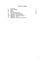
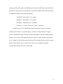
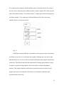
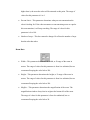
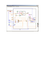
The robot is designed to output its coordinates, and then it waits for a
concentration reading at those coordinates. The dispersion model takes in the robot’s
coordinates and produces a concentration. This concentration is passed to the Enose
module, which creates the requested concentration and passes it through its sensor
chamber. The sensors then produce a voltage response, which corresponds with some
concentration. This response is passed back to the robot. Using this response, the robot
decides where to move next, and the cycle continues. This can be seen in the following
illustration.
3
Fig. 1.1
We chose to implement our system in LabVIEW, because this was the language
that the Enose interface was written in. The following documentation explains the steps
we took and decisions we made to complete our task.
4
II. Dispersion Module
The dispersion module is essential to this project. This is the module that models
the odor source, and the concentration of odor at any point in the environment. It is
necessary for this model to be accurate, so that we will be able to tell the effectiveness of
our robot in a realistic situation. In our research of odor dispersion models, three models
had potential.
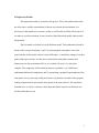
The first model we looked at was the Eulerian model. This mathematical model is
based on the concept of tracking a “puff” of gas through the atmosphere. One of the
major benefits of this model is that it is time differential – it models the change of an odor
plume with respect to time. As time moves forward, the odor plume stretches and
disperses across the environment. This is very realistic. However, it is also quite
complex. The complexity of this model presents two problems: 1) it is difficult to
understand and therefore implement, and 2) regenerating a graphical representation of the
odor plume at every time step would put a massive lag into the execution of the program,
making it impractical to represent the odor plume as the robot tracks it. The equation is
included here, as well as a reference, in the hope that future research can find more use
for this model than we can.
5
Fig. 2.1 (Zannetti)
2Qqh a
0
c ( x, z ) =
+
a
1
h
u
0
c ( x, y , z ) = c ( x, z )
σ 2 q 2 K x
z0
γ i
−
q
σ
q
J
λ hru
p γ − 1 γ (i ) R J y − 1 σ γ i (z h )
h
zR
•e
0 0
∑
λ
+
h
2 σ
J
γ − 1 γ i
1
2πσ
e
−
y2
2σ 2
y
y
Eq. 2.1 (Zannetti)
6
The second model we looked at was the Lagrangian model. It was very similar to
the Eulerian model. The major difference between the two was that the Eulerian model
represented the puff of air moving with relation to the environment, while the Lagrangian
model represented the environment moving in relation to the puff of air. This is
illustrated in the following figure.
Fig. 2.2
(Zannetti)
The equations for this model are given below.
c(r , t ) =
A(r ) =
A(r ) n
∑ miW (ri − r , l )
l 3 i =1
l3
∫ W (r '−r , l )dr '
D
W (ri − r , l ) =
1
(2π )3 / 2
e
1 r −r
− i
2 l2
2
Eq. 2.2 (Zannetti)
7
Again, these equations are given solely for the benefit of future researchers.
The model we chose to use is the Gaussian model. This model is a statistical
model, and is much simpler than the previous two models. The main drawback is that it is
not as realistic, because it is not time differential. It calculates the concentration at each
point in the room under the assumption that the odor has had sufficient time to diffuse
through the room. However, this presents an advantage over the other two models in that
a graphic for this model can be generated once and then the movement of the robot can
be mapped onto it repeatedly. The equation for this model is given below.
c ( x, y , z ) =
Q
2πσ σ
y z
e
1 y r
−
2 σ
y
2
1 he − z r
−
2 σ
z
e
2
Eq. 2.3 (Zannetti)
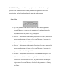
The basic idea behind this model is that the odor concentration follows a normal
distribution in the Y and Z directions, with the middle of the distribution being along the
X-axis. The terms σY and σZ determine the shape of these normal distributions. The terms
σY and σZ are based upon the stability of the atmosphere and the distance from the source
in the X direction. The equations for σY and σZ then become:
Xdist
σY = A •
1000
0.894
D
Xdist
σZ = C •
−F
1000
8
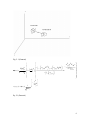
Where A, C, D, and F are all constants derived from the estimation provided by
industialhygiene.com. See Gauss.c for a more complete explanation. The concentration
follows a logarithmic curve down the X-axis, decreasing exponentially as it gets farther
from the source. Zannetti provides an excellent illustration of this in the figure below.
Fig. 2.4 (Zannetti)
9
The major limitation for us was the fact that, as you approach the origin, or the
location of the odor source, the concentration approaches infinity. This presents two
problems. First of all, this is obviously not realistic. Second, because of the logarithmic
nature of the model, there is a very steep concentration gradient in a very small area
surrounding the source, and practically no gradient anywhere else. This makes it very
difficult for the robot to pick up a change in concentration unless it is right next to the
source. This ‘infinity’ problem arises from the fact that σY and σZ approach zero as X
approaches zero.
To correct this behavior, we limited σY and σZ so that if they went below 0.1, they
would be set to 0.1. This effectively chopped off the top of the model at a certain height.
The problem with this solution is that it creates an amount of distortion; the higher the
cutoff of σY and σZ, the greater the distortion. However, the lower the cutoff, the greater
the peak, and the greater the gradient. To solve this problem, we set σY and σZ very low,
and the cut off the concentration if it got above a certain percentage of the maximum
concentration. This created an effective ‘cap’ on our concentration, and also made it so
that the gradient was not so steep that the robot could not find it at long distances. We
made this ‘cut-off’ percentage an input into the model so that it could be assigned
dynamically between runs of the program.
We further simplified the model by assuming that the robot would be sampling on
the ground, and therefore the Z term was useless, thus making our dispersion model a
2 dimensional model. Our code implementation can be found in Gauss.c.
10
III. Robot Algorithm
The robot algorithm is used to simulate the behavior of a robot in an environment
with an arbitrary number of odor sources. Given the geometry of the room, the robot will
execute an algorithm that will follow odor gradients toward a source. This algorithm
uses three phases to initialize the robot, and one stage to follow gradients. The first three
stages move the robot in a circle, gathering concentrations at the circumference. Based
upon these samples, it determines the direction of highest concentration increase, and
begins moving in that direction. The fourth stage is the main stage, and this is where the
robot spends most of its time. Here, it calculates a momentum vector and determines its
next move. The fifth stage is used to guide the robot in the right direction once it begins
to lose the gradient of the odor plume.
At all times, the robot is keeping track of three points; the point it was just at
(Ref_point), the point it is at now (Cur_point), and the point in its history that has had the
highest concentration (Max_point). It also remembers the concentration at all of these
points. This is necessary for the calculation of the next move.
Stage 0 simply sets the values for key variables. The dimensions of the room are
stored, and the current point is set. The direction of the robot is set to zero, and all
internal memory of points is erased. This stage is actually done twice, to clear erroneous
data from the sensors. The second time, the stage is set to Stage 1.
In Stage 1, the robot samples the concentration at its starting point. It then moves
forward, and stage is set to Stage 2.
In Stage 2, the robot gathers an odor sample. The robot then returns to the
starting point, turns 135° counter-clockwise and takes another step outward. This process
11
repeats until the robot has made an 8-point circle around the starting point. From this
phase, the robot gathers the point of highest concentration from the starting point. This is
used in Stage 3 to set an initial momentum vector, so the robot will start off moving in
the direction of highest concentration.
Stage 3 is the main movement phase. In this phase, the robot uses the alpha and
beta parameters to calculate a new momentum vector. The direction of the momentum
vector is the direction in which the robot “thinks” it should move. The magnitude of this
vector is not a distance, but a change in concentration. To generate a new momentum
vector at each point, there are three steps. In the first step, the current direction of the
robot and the current change in concentration from the last point are used to define a
temporary vector. This vector is added to the previous momentum vector to determine X
and Y components of the new momentum vector. This is done using the following
equation.
TempVectorX = (1 - alpha) * deltaConc * cos(theta * (pi/180))
TempVectorY = (1 - alpha) * deltaConc * sin(theta * (pi/180))
NewMomentumVectorX = (alpha * ||OldMomentumVector||) + TempVectorX
NewMomentumVectorY = TempVetorY
Here, theta is the amount of “wiggle” the robot has. This will be explained later.
After this, we can figure out how far the robot needs to turn to point itself in the
direction of this new momentum vector. We do this using the following equation.
DeltaAngle = arctan(NewMomentumVectorY/NewMomentumVectorX);
So now we know how far to turn our robot. In the second step, the direction of the
robot is modified based on the robots position with relation to Max_point. If the robot is
12
facing away from Max_point, it should turn to face more towards Max_point. Beta is the
parameter in control of how much the robot’s direction is modified. The robot’s direction
is modified according to the following equation.
maxDistX = Max_point.x - Cur_point.x
maxDistY = Max_point.y - Cur_point.y
maxAngle = atan(maxDistY / maxDistX)
Direction = (1 - beta) * Direction + (beta) * maxAngle
At this point, we have calculated the direction in which we believe the robot
should go next. However, to test this theory, we add in a certain amount of “wiggle”,
which is determined by theta. We turn our robot theta degrees, and then multiply theta by
negative one to make it in the opposite direction. This way, when it adds theta next time,
it will “wiggle” the robot in the opposite direction. This wiggle allows the robot to choose
the best route, instead of just a “good” route, because it is constantly testing the
concentration on either side of it’s chosen path.
13
IV. LabVIEW
Since our project was entirely simulated, we had to decide on a programming
language to create the simulation in. We chose to do the majority of the project in
LabVIEW since the existing dilution system’s interface was written in LabVIEW. We
also chose to write the code for our dispersion module and our robot simulation in C and
then integrate it into LabVIEW. In LabVIEW you can create a VI and then insert it into
another VI as a sub-VI. We took advantage of this capability so that we could break up
the code and easily integrate the separate parts. Sub-VIs also allow you to make changes
easily since you only have to make changes in one VI and then the changes carry on to all
the other VIs that include that changed VI.
To use C code in conjunction with LabVIEW, we had to use LabVIEW’s CIN
modules. Please refer to Appendix D for steps on how to build the CIN code resource for
the CIN module. When you insert this module, you create all the inputs and outputs in
LabVIEW and then create a C source code file by right-clicking the module and selecting
“Create .c file.” This creates the C source code file with all the correct inputs and outputs
and even tells you where to enter your code. You enter the code that you want executed
and then proceed with the steps to compile the code and build the code resource file (.lsb
file). You can then load the code resource file into the CIN module and then run your VI.
Any inputs to the VI will be run through the C code, and then the C code will set the
module’s outputs.
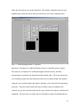
Our main VI is called “OdorTrackingSoftware.vi.” This VI includes all of our
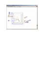
interface and all of the other sub-VIs. The interface (Figure 4.1) allows the user to input
14
all the necessary input to set up the simulation. This includes setting the room size and
magnification, setting the source data for all the sources to be used, setting the robot
Fig. 4.1 “OdorTrackingSoftware.vi” interface.
parameters, choosing to use either the dilution system or a simulated sensor response.
The room size is composed of a width and length measured in meters, and these
measurements are passed to the dispersion module and the robot. The room is then used
as a coordinate system where the bottom left corner is (0,0) and the width is the distance
along the x-axis and the length is the distance along the y-axis with each increment being
one meter. The source data includes the source location (x and y-coordinates), the
emission rate (Q), the wind direction from the source (measured in degrees), and the wind
magnitude. The user can use as many sources as desired by simply incrementing the top
15
index in the two-dimensional source data array. The robot parameters include the robot’s
starting location (x and y-coordinates), a weighted parameter (alpha) that controls how
much the robot follows its past movements as opposed to its new movements, a weighted
parameter (beta) that controls how much the robot veers towards the highest point of
concentration so far, and the percent limit, which tells the robot to stop once it has
reached a concentration that is at least that percentage of the maximum concentration
value. There is also a button that allows you to either use the existing dilution system, to
use real sensor responses, or to use simulated sensor responses to observe the robot’s
behavior in an ideal situation.
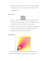
There are also two displays to show the results. One is a plot that shows an
overhead view of the room, the odor source and plume, and the robot’s location and path
each step along the way. The other display graphs both the concentration percentage
from the dispersion model and the sensor response-based concentration from the dilution
system. The left y-axis correlates to the relative concentration (yellow line) from the
sensor responses. The right y-axis correlates to the concentration percentage (green line)
from the dispersion model. Time is measured on the x-axis.
We also use a VI called “Concentration.vi.” This VI is composed of to connected
sub-VIs, “Gauss.vi” and “Convert.vi.” “Gauss.vi” contains the CIN module for the
dispersion module. It takes in as input a location (x and y-coordinates) and the source
data, and it calculates a corresponding concentration value. Since the Gaussian model
puts the source at location (0,0) and the wind blowing in the positive x-direction, we
needed to have a conversion module to correlate the correct points in the room with the
correct points in the Gaussian model. “Convert.vi” takes in the actual location and source
16
data and generates a “converted” location relative to the Gaussian model.
“Concentration.vi” takes in a location (x and y-coordinates), the source data, and the
room data, and it generates the concentration at that location.
To create the visual odor plume, we created a VI called “DispersionModule.vi."
This VI runs the “Concentration.vi” through two for loops to generate the concentration
at each point in the room. These concentrations are kept in an array, which is then sent
through a LabVIEW module that creates an 8-bit picture from all the values. This
module takes the concentrations as numbers and draws a colored dot at that location,
where the color depends on the concentration value. This produces color gradients that
mimic the concentration gradients of the odor plume. This picture is then passed to the
display, which then maps the robots points on top of the picture. This VI also outputs the
maximum concentration calculated.
Another VI we created is called “PercentProfile.vi.” This VI takes in the
concentration from the dispersion model and the maximum concentration. It then
calculates the concentration as a percentage of the maximum concentration. The dilution
system has a dilution profile as an input, which tells the diluters what concentration to
generate. This dilution profile is a two-dimensional string array of concentration values,
where the sub-array contains the percentage values for the three diluters.
“PercentProfile.vi” takes the percentage it has calculated, converts it into a string, and
then populates an array with three copies of this value. This array is then added to a twodimensional array to be passed to the dilution system.
The final VI we used was called “enose_interface.vi.” This is the interface to the
dilution system that was created during a previous semester. We basically kept this VI
17
like it was except for a few minor changes to give us the output we needed. We added
some functionality that allows us to retrieve the average sensor response over the middle
third of the sensing time, since we found this region of the response to be the most stable.
The only other VIs that we changed were some of the plot VIs that control the display of
the room with the odor plume and robot. We removed various characteristics, such as
rescaling the axis and drawing the axes.
V. Enose System Description
The dilution system was developed by a group of previous students. It basically consists
of three gas diluters, a mixing chamber, a pump and circuit. It takes different gases as inputs, and
outputs the average voltage of the four sensor signals. For detailed information about this system,
please look at the User’s Manual of the E-nose Odor Delivery System (Appendix A).
VI. Integration with E-nose System:
How our robot simulator integrates with the existing odor mixing system is one of
the main parts of our project. The dilution system cannot run continuously for a long
time, like an hour, because the hardware can be burned out. For the effective testing
purposes, we have implemented different odor tracking algorithms and many other things
within our LabView model. We choose the tracking algorithm that has the least running
time to find the source so we can test it with the dilution system.
For the simplicity, we just use one analyte, Isopropyl alcohol, in all our tests.
Serial hook up for the dilution system:
18
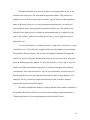
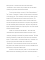
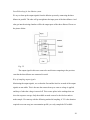
We tested the robot simulator with the dilution system connected in serial. We connect
the odor source to the input port of diluter number 1 and its output will be hook up as the
input of the diluter number 2. The diluter number 2’s output port will be the input port of
the diluter number 3. The output port of the third diluter will be fed in the mixing
chamber. Please see the picture below:
Fig. 5.1
Each diluter can only dilute the concentration to one part per twenty. By hooking
the diluters up in series, we are theoretically capable of diluting up to one part in eight
thousand. However, we ran several tests and noticed that the output signals contained too
much noise. The diluter manual had the instructions for hooking up the diluters in series.
It requires a separate mixing chamber, with an air intake to maintain atmospheric
pressure. This separate chamber would ruin our results because the air intake would
produce an incorrect concentration. This incorrect concentration makes the robot
simulator behave incorrectly.
19
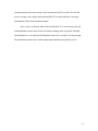
Parallel hook up for the dilution system:
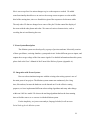
We try to clean up the output signals from the dilution system by connecting the three
diluters in parallel. The odor will go straight into the input ports of the three diluters. And
odor get into the mixing chamber will be the output ports of the three diluters. Please see
the picture below:
Fig. 5.2
The output signal in this case seem to be much better comparing to the previous
case that the three diluters are connected in serial.
Way of sampling output signals:
Monitoring the output signals, we see that the first and the last few seconds of the output
signals are not stable. This is because the sensors heat up as soon as voltage is applied,
and drop of when the voltage is turned off. This creates spikes in the readings that can
skew the response average. Only the middle seconds seem to be the ideal seconds to
make sample. We came up with the following method of sampling: if ‘D’ is the duration
required to run one step (one concentration profile), we only sample the D/3 middle
20
seconds and don’t take into account of the first and the last D/3 seconds. We take the
inverse average of the voltage during that middle D/3 seconds and make it the input
concentration of the robot simulation model.
Also, we have to find out what is the best duration ‘D’ to run one step since the
existing dilution system needs to have the shortest running time as possible. Through
experimentation, we see that the ideal duration seem to be 6 seconds. It is long enough
for the dilution system to have stable output signal and short enough for it to run.
21
User manual
Basic Operation
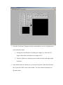
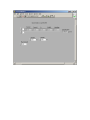
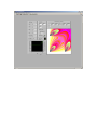
1. To run the most basic version of our system, open LabVIEW. A window similar
to Fig. 1 below should appear.
Fig. 1
2. Select Open. A File selection window will appear.
3. Make sure the CD is in your CD drive.
Open D:\LabVIEW\OdorTrackingSoftware.vi
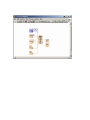
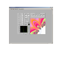
4. A window should appear like Figure 2 below.
5. Press the “Use E-nose” button to use the e-nose hardware, or leave it deselected to
run in simulation mode.
a. If using the e-nose hardware, turn the power supply on. Select the 25V
output, and use the scroll wheel to set output to 12V.
b. Turn the 3 diluters on, using the power switches located in the upper right
of the box.
6. Since default values are already set, you can select Operate>>Run from the menu
bar, or press the “Run” arrow on the toolbar. For more advanced operation, see
the next section.
7. If the E-nose is activated, the pump will turn on, and the sensors will have a 10
second warm-up period before executing the simulation. The system will then
generate the odor dispersion profile and plot the graph on the right. As the robot
begins to run, the display will update to plot the position of the robot.
8. If the e-nose is deactivated, the system will generate the dispersion profile and
begin running the robot code to track the odor.
Advanced Operation
Robot Data
•
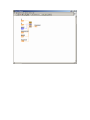
Start Coordinates - The robot has controls for selecting the starting position in
X and Y coordinates, as seen in Figure 3. These are measured from the
bottom left corner of the graph, in meters. The range for these values must be
less than the size of the room
•
Alpha – The alpha parameter is the robot’s momentum parameter. The higher
the value of alpha, the greater the robot’s tendency to continue in a straight
line. The lower the value of alpha, the more responsive the robot will be to
changes in concentration. The range of values for this parameter is 0 to 1.
•
Beta – The beta parameter determines how strongly the robot is attracted to
the point with the highest concentration it has experienced thus far. The robot
remembers which point it has visited that has the highest concentration. The
higher beta is, the more the robot will be attracted to this point. The range of
values for this parameter is 0 to 1.
•
Percent Limit – This parameter determines what percent concentration the
robot is looking for. If the robot encounters a concentration greater or equal to
this concentration, it will stop searching. The range of values for this
parameter is 0 to 100.
•
Number of steps – This box cannot be changed. It reflects the number of steps
that the robot has taken.
Room Data
•
Width – This parameter determines the width, or X range of the room in
meters. The range of values for this parameter is from 0 to unlimited, but we
recommend keeping the value below 500.
•
Height – This parameter determines the height, or Y range of the room in
meters. The range of values for this parameter is from 0 to unlimited, but we
recommend keeping the value below 500.
•
MagFac – This parameter determines the magnification of the room. The
magnification window always has its origin at the bottom left of the room.
The range of values for this parameter is from 0 to unlimited, but we
recommend keeping the value below 20.
!CAUTION! – The generation of the odor graphic requires width * height * magfac
cycles to create. Setting the values of these parameters to high values can increase
generation time, and add significant lag to the start time of the program.
Source Data
•
Q – This parameter is the emission rate of the source in micrograms per
second. The range of values for this parameter is 0 to unlimited, but values
beyond 100,000 do not produce very good graphics.
•
SourceX – This parameter is the starting X position of the source, measured in
meters from the bottom left corner of the room. The range of values for this
parameter is from 0 to the width of the room.
•
SourceY – This parameter is the starting Y position of the source, measured in
meters from the bottom left corner of the room. The range of values for this
parameter is from 0 to the height of the room.
•
WindDir – This parameter determines the direction that the odor plume will
blow in, measured in degrees. For example, if the odor is in the center of the
room and the wind direction is set to 45, the plume will blow into the upper
right corner of the room. The range of values for this parameter is –infininty
to infinity.
•
WindMag – This parameter determines the velocity of the wind. The range of
values for this parameter is >0 to unlimited, but we recommend keeping the
value between 1 and 6.
E-nose Controls
•
Use Enose? – This button determines if the Enose system will be used, or if
the system will run in simulation mode. If the button is highlighted green, then
the Enose system will be used. The default is to run in simulation.
•
Step duration – This parameter determines the duration of the sample that the
Enose system will take. The range of values for this parameter is from 0 to
unlimited, but we have found that 6 seconds is optimal.
Simulation Display
This is the main display window, where the odor model is graphed, and the
movement of the robot is displayed. The lower right corner of the graph can be
stretched with the right mouse button in order to enlarge the display area to any size.
By right clicking on the graph with the mouse, you can go to Data Operations and
then Clear Graph to clear the graph if desired between runs of the system.
Sensor Display
On this graph, real-time readings of the odor model and sensor concentration
readings are displayed in yellow and green. Yellow represents the data given by the
dispersion model, and green represents data coming in from the odor sensors.
Clicking on the top number and typing in the desired maximum axis value can adjust
the scale on the right and left of the graph. The scroll bar at the bottom can be used to
scroll backwards to review data readings from previous executions of the system. By
right clicking on the chart with the mouse, you can go to Data Operations and then
Clear Chart to clear the graph if desired between runs of the system.
Course Debriefing
Group Management Style
For the most part our group management worked well. We feel that we started off
a bit too disorganized, and should have worked together more often per week to
synchronize efforts and make sure all team members were caught up with all
developments. We think we probably should have had more weekly group meetings
amongst ourselves in order to synchronize our efforts and discuss developments and next
steps to take. Later in the project, we also began meeting with our project advisors two to
three times a week rather than one, in order to speed development, and set goals in a
more rapid manner. We found these meetings to be extremely helpful, because they
allowed us to get more feedback and advice about the project in a more rapid manner.
This also helped with the aforementioned problem of keeping all team members up to
date.
Safety and Ethical Concerns
Since our e-nose hardware requires the use of dilutions of chemicals such as ethyl
alcohol and ammonia, we were instructed by our advisors not to deal with filling the
chemical mixing chambers or adjust the dilution ratios. Instead, one of our advisors,
Agustin Gutierrez-Galvez was asked to refill mixing chambers if needed.
Product Testing
We did extensive testing on our product. Initially we tested the robot code in a
simulation mode, without using the e-nose hardware. This allowed us to at least verify
the correctness of the tracking algorithm in idealized conditions, without having to be
concerned with the realities of the e-nose hardware. When we felt fairly confident on the
correctness of the odor tracking algorithm, we began testing the algorithm with the e-nose
hardware in the test loop. We also ran tests on the e-nose hardware by itself, so we could
test sensor response using simple concentration profiles. Some of the profiles we tried
were increasing ramp, decreasing ramp, hill, and valley profiles. These were all tested in
order to see how the sensors responded using various sample time periods. We also
tested flushing the sensors with pure air at a higher voltage between analyte readings, to
see if this method would clean out the sensors and achieve better readings. We found
that it did not significantly improve the sensor output levels. We also tested connecting
the sensors in series and in parallel modes. It was initially believed that connecting the
sensors in series would allow us to achieve a finer degree of control over the exactness of
the concentration. However due to air pressure and voltage changes in the system, it was
found that this solution created sinusoidal variations in the output signal, which are
undesirable and create unusable data for our system. After consulting the diluter
manuals, it was also found that additional equipment would be required to properly
connect the diluters in series. To use this hardware would mean using an intermediary
mixing chamber for the analyte, which would take in an unspecified amount of room air.
This of course is unusable in our system, since we need exact measurements of analyte
dilution.
We feel we have been fairly thorough in testing our system, with arbitrary number
and strength of odor sources. We have also tested our code with and without the
hardware.
Limitations of the System
The system does have a few limitations. It requires no less than three seconds to
sample the odor. Also, there is a bit of a lag in the response of the sensors to the change
in analyte concentration. The robot is not flawless, either. When it crosses the gradient
perpendicular to the axis of dispersion, it has a difficult time choosing where to go.
Sometimes it gets lost, and performs in an apparently nonsensical fashion. It does not
filter the data from the Enose, but uses it raw, which can produce skewed results.
Future Development
In the future, hopefully this system will be implemented in an actual robot. Other
aspects that could be improved by future groups are the response and recovery time of the
sensors, the accuracy of the sensors, the precision of the diluters, and the tracking
algorithm of the robot.
/*********************************
*
* Robot.c
*
* Written by:
* Simon Saugier
* Jason Hamor
* Greg Allbee
* Ninh Dang
*
* CPSC 483, Senior Design
* Spring 2003
*
**********************************
/************************************
*
* The purpose of this code is to simulate the behavior of a robot
* in an environment with an arbitrary number of odor sources. The
* goal of the robot is to detect odor gradients and use these to
* track down the location of an odor source. The robot uses a
* weighted movement algorithm to account for a sense of "momentum"
* based on past history, as well as to account for its' knowledge
* of the highest point concentration seen thus far.
*
************************************************************
#include "extcode.h"
#include <stdio.h>
#include <stdlib.h>
#include <math.h>
/* Data structure used to define a point in terms of (x,y) position and a
concentration at that point
*/
typedef struct {
float32 x;
float32 y;
float32 Conc;
} point;
/* Data structure to define a momentum vector of the robot, based on the
current direction and a confidence number representative of how "sure"
the robot is that it is moving in the right direction.
*/
typedef struct {
int dir;
float conf;
} Momentum_Vector;
int stage = 0;
int gdir = 0;
int i = 0;
int theta = 20;
int XMAX, YMAX;
float m,curStep,minStep,maxStep;
float pi = 3.1415926535897;
point C[8];
int D[8];
LVBoolean found = LVFALSE;
point Cur_point;
point Ref_point;
point Max_point;
Momentum_Vector MV;
void turnAround ();
void turnLeft();
void turnRight();
void turn(int degree);
void inBounds();
void moveForward (float32 dist);
/*
CINRun is the procedure called by LabVIEW when it finds a CIN on the block
diagram.
*/
CIN MgErr CINRun(float32 *StartX, float32 *StartY, float32 *Concentration,
int32 *Width, int32 *Length, float32 *NextX, float32 *NextY,
LVBoolean *Reset, float32 *Alpha, float32 *Beta);
CIN MgErr CINRun(float32 *StartX, float32 *StartY, float32 *Concentration,
int32 *Width, int32 *Length, float32 *NextX, float32 *NextY, LVBoolean *Reset,
float32 *Alpha, float32 *Beta) {
float MaxConc = 0;
int j,c,index = 0;
float deltaConc, Vx, Vy, RVx, RVy;
double deltaAngle, maxAngle;
float alpha = 0.5;
float beta, maxDistX, maxDistY;
if (*Reset)
{
stage = 0;
c = 0;
*Reset = LVFALSE;
}
/*
This case statement is used to guide the robot through several "stages" of
odor tracking. The first stage, stage 0, is used to set initial values for
the robot variables.
Stage 1 is used to get the robot to take the first step towards the right,
and to set the initial reference point of concentration.
Stage 2 makes an 8-point circle around the initial point. It takes a sample
at each of these points, and uses the point of highest concentration as a reference
point.
Stage 3 is the main movement stage. A calculation is made for an Alpha parameter,
which keeps track of recent history using momentum. Then a calculation is made
based on the absolute maximum concentration sensed by the robot so far. The decision
of where to move next is based on a weighted average of these two vectors. The
movement
(step) size is also scaled based on the confidence vector, so that larger steps can be
taken when the odor gradients are low, and small steps taken when the odor gradients
are
high, and hence close to the source.
*/
switch (stage)
{
case 0:
XMAX = *Width;
YMAX = *Length;
if (XMAX > YMAX){
minStep = YMAX / 100;
maxStep = YMAX / 20;
} else{
minStep = XMAX / 100;
maxStep = XMAX / 20;
}
gdir = 0;
m = maxStep;
Ref_point.x = *StartX;
Ref_point.y = *StartY;
Cur_point = Ref_point;
i = 0;
if (c==0)
stage = 0;
else stage = 1;
c++;
break;
case 1:
Ref_point.Conc = *Concentration;
moveForward(m);
inBounds();
i = 0;
stage = 2;
break;
case 2:
Cur_point.Conc = *Concentration;
C[i] = Cur_point;
D[i] = gdir;
i++;
if(i>7)
{
MaxConc = C[0].Conc;
index = 0;
for(j=0;j<8;j++)
{
if(C[j].Conc > MaxConc)
{
MaxConc = C[j].Conc;
index = j;
}
}
turnAround();
moveForward(m);
gdir = D[index];
moveForward(m);
Ref_point = Cur_point;
MV.conf = C[index].Conc - Ref_point.Conc;
MV.dir = D[index];
gdir = gdir + theta;
moveForward(m);
Max_point.Conc = 0;
Max_point.x = 0;
Max_point.y = 0;
stage = 3;
break;
}
turnAround();
moveForward(m);
turn(135);
moveForward(m);
break;
case 3:
Cur_point.Conc = *Concentration;
alpha = *Alpha;
beta = *Beta;
if (Cur_point.Conc > Max_point.Conc)
Max_point = Cur_point;
// recent history calculations
deltaConc = Cur_point.Conc - Ref_point.Conc;
Vx = (1 - alpha) * deltaConc * cos(theta * (pi/180));
Vy = (1 - alpha) * deltaConc * sin(theta * (pi/180));
RVx = (alpha * MV.conf) + Vx;
RVy = Vy;
if (RVx == 0)
{
if (RVy == 0)
deltaAngle = 0;
else deltaAngle = 90;
}
else
{
deltaAngle = (180/pi) * atan(RVy / RVx);
}
if (theta * deltaConc >= 0)
{
MV.dir = MV.dir + deltaAngle;
}
else
{
MV.dir = MV.dir - deltaAngle;
}
// end recent history calculations
// Max point calculations
maxDistX = Max_point.x - Cur_point.x;
maxDistY = Max_point.y - Cur_point.y;
if (maxDistX == 0){
if (maxDistY > 0)
maxAngle = 90;
else if (maxDistY < 0)
maxAngle = 270;
else
maxAngle = 0;
}
else
maxAngle = (180/pi) * atan(maxDistY / maxDistX);
if (maxDistX < 0)
maxAngle = maxAngle + 180;
if (abs(maxAngle - MV.dir) > 180)
maxAngle = maxAngle - 360;
if ((Max_point.x != Cur_point.x) && (Max_point.y != Cur_point.y) &&
(Max_point.Conc != 0))
{
MV.dir = (1 - beta) * MV.dir + (beta) * maxAngle;
}
// end of max point calculations
MV.conf = sqrt( RVx*RVx + RVy*RVy );
// scale step size according to magnitude of momentum vector.
curStep = 15 * (1 / MV.conf);
if (curStep < minStep)
curStep = minStep;
else if (curStep > maxStep)
curStep = maxStep;
m = curStep;
*Confid = m;
Ref_point = Cur_point;
theta = theta * -1;
gdir = MV.dir + theta;
moveForward(m);
inBounds();
break;
} // end of switch statement
*NextX = Cur_point.x;
*NextY = Cur_point.y;
return noErr;
} // end of CINRun
/* turn(degree) turns the robot to face an arbitrary angle */
void turn( int degree)
{
gdir = gdir + degree;
}
/* turnAround() uses the current heading of the robot and turns 180 degrees */
void turnAround ()
{
gdir = (gdir + 180) % 360;
}
/* turnLeft() turns the robot 90 degrees to the left of the current heading */
void turnLeft()
{
gdir = (gdir + 90) % 360;
}
/* turnRight() turns the robot 90 degrees to the right of the current heading */
void turnRight()
{
gdir = (gdir + 270) % 360;
}
/*
moveForward(dist) take in an absolulte distance as a float, calculates
the delta in x and y using that distance and the current direction,
then sets the new current point location.
*/
void moveForward (float32 dist)
{
float32 delta_x;
float32 delta_y;
delta_x = dist*cos((gdir*pi)/180);
delta_y = dist*sin((gdir*pi)/180);
Cur_point.x = Cur_point.x + delta_x;
Cur_point.y = Cur_point.y + delta_y;
}
/*
Procedure inBounds() uses the global Cur_point.x and Cur_point.y
to determine if the current location is within the bounds of the
known room. If they are not, we reset our position to something
in bounds and reset the MV.dir.
*/
void inBounds()
{
if (Cur_point.x < 0)
{
gdir = 180 - gdir;
MV.dir = gdir;
Cur_point.x = 0;
}
if (Cur_point.y < 0)
{
gdir = 360 - gdir;
MV.dir = gdir;
Cur_point.y = 0;
}
if (Cur_point.x > XMAX)
{
gdir = 180 - gdir;
MV.dir = gdir;
Cur_point.x = XMAX;
}
if (Cur_point.y > YMAX)
{
gdir = 360 - gdir;
MV.dir = gdir;
Cur_point.y = YMAX;
}
} // end of inBounds()
/*********************************
*
* Gauss.c
*
* Written by:
* Simon Saugier
* Jason Hamor
* Greg Allbee
* Ninh Dang
*
* CPSC 483, Senior Design
* Spring 2003
*
**********************************
#include "extcode.h"
#include <math.h>
CIN MgErr CINRun(float32 *Xcoor, float32 *Ycoor, int32 *Stability, float32 *Q,
float32 *WindMag, float32 *Concentration, float32 *MaxConcLimit);
CIN MgErr CINRun(float32 *Xcoor, float32 *Ycoor, int32 *Stability, float32 *Q,
float32 *WindMag, float32 *Concentration, float32 *MaxConcLimit) {
float pi, e;
float ConstA, ConstC, ConstD, ConstF;
float sigmaY, sigmaZ;
float Max, Qu, WM;
pi = 3.1415926535897;
e = 2.718281828;
Qu = *Q;
WM = *WindMag;
if(*Stability<0) *Stability = 0;
if(*Stability>5) *Stability = 5;
switch (*Stability) {
case 0:
ConstA = 213;
if (*Xcoor <= 1000) {
ConstC = 440.8;
ConstD = 1.941;
ConstF = -9.27;
} else {
ConstC = 459.7;
ConstD = 2.094;
ConstF = 9.6;
}
break;
case 1:
ConstA = 156;
if (*Xcoor <= 1000) {
ConstC = 106.6;
ConstD = 1.149;
ConstF = -3.3;
} else {
ConstC = 108.2;
ConstD = 1.098;
ConstF = -2.0;
}
break;
case 2:
ConstA = 104;
ConstC = 61.0;
ConstD = 0.911;
ConstF = 0;
break;
case 3:
ConstA = 68;
if (*Xcoor <= 1000) {
ConstC = 33.2;
ConstD = 0.725;
ConstF = 1.7;
} else {
ConstC = 44.5;
ConstD = 0.516;
ConstF = 13.0;
}
break;
case 4:
ConstA = 50.5;
if (*Xcoor <= 1000) {
ConstC = 22.8;
ConstD = 0.678;
ConstF = 1.3;
} else {
ConstC = 55.4;
ConstD = 0.305;
ConstF = 34.0;
}
break;
case 5:
ConstA = 34;
if (*Xcoor <= 1000) {
ConstC = 14.35;
ConstD = 0.740;
ConstF = 0.35;
} else {
ConstC = 62.6;
ConstD = 0.180;
ConstF = 48.6;
}
break;
}
sigmaY = ConstA * pow((*Xcoor/1000),0.894);
sigmaZ = ConstC * pow((*Xcoor/1000),ConstD)-ConstF;
if(sigmaY < 0.1) sigmaY = 0.1;
if(sigmaZ < 0.1) sigmaZ = 0.1;
*Concentration = -1;
if(*WindMag <= 0) *Concentration = 0;
if(*Xcoor < 0 ) *Concentration = 0;
Max = (Qu/(pi*0.1*0.1*(WM)));
if(*Concentration < 0) {
*Concentration = (Qu/(pi*sigmaY*sigmaZ*(WM)))*pow(e,(0.5*pow((*Ycoor/sigmaY),2)));
}
if(*Concentration > (*MaxConcLimit) * Max) {
*Concentration = (*MaxConcLimit) * Max;
}
return noErr;
}
How to build a CIN code resource (.lsb file) - Tutorial - Developer Zone - National Instru... Page 1 of 6
NI Home | MyNI | Site Help | My Profile | Contact NI
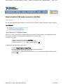
How to build a CIN code resource (.lsb file)
Back to Document
This document details the steps necessary to create a CIN code resource (.lsb file) using the following compilers:
Table of Contents:
z
z
z
Microsoft Visual C++ v. 5.0 for Win32 platforms
CodeWarrior for PowerPC platforms
Gnu C compiler for Solaris platforms
Microsoft Visual C++ v. 5.0 for Win32 platforms
Visual C++ 5.0 has a Custom Build capability that allows you to build CINs from within the Integrated Developer
Environment. Complete the following steps to generate the "VI_name.lsb" file.
1) Create a DLL project.
A. Make a new project by selecting File>>New.
B. Specify the type to be "Win32 Dynamic-Link Library."
C. Name the project "VI_name", with no spaces, and click OK.
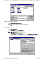
2) Add CIN objects and libraries to the project.
A. Select Project>>Add To Project>>Files.
B. Go to the Win32 subdirectory of your cintools directory and select
cin.obj, labview.lib, lvsb.lib, and lvsbmain.def
C. You can select multiple items by holding down the <Ctrl> button and clicking the items you want.
Then click OK.
mhtml:file://I:\tmp1\Appendix%20D.mht
5/12/2004
How to build a CIN code resource (.lsb file) - Tutorial - Developer Zone - National Instru... Page 2 of 6
3) Add your "VI_name.c" file to the project.
A. Select Project>>Add To Project>>Files.
B. Go to the folder that holds your "VI_name.c" file and select it.
C. Click OK.
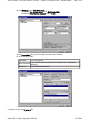
4) Edit Project Settings.
A. Select Project>>Settings.
B. Set the Settings For field to All Configurations.
C. The remaining sub-steps are all within this panel:
Do not click the OK button until instructed to do so later.
On the C/C++ tab:
- Set the Category field to Preprocessor.
- Add the absolute path to your cintools directory in the Additional include directories field.
Paths should either be in MS-DOS format or have quotes surrounding the entire path.
mhtml:file://I:\tmp1\Appendix%20D.mht
5/12/2004
How to build a CIN code resource (.lsb file) - Tutorial - Developer Zone - National Instru... Page 3 of 6
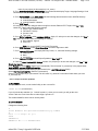
Set the Category field to Code Generation.
-Change the Use run-time library field to Multithreaded DLL.
-Change the Struct member alignment field to 1 Byte.
On the Custom Build tab, scroll to the right to find the custom build tab.
Fill in the following fields:
Description:
Fill in a description.
Build commands
"<your Cintools path>\win32\lvsbutil" "$(TargetName)" -d "$(WkspDir)
\$(OutDir)"
Output files
"$(OutDir)$(TargetName).lsb"
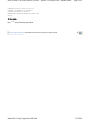
5) Add your code to the VI_name.c file.
mhtml:file://I:\tmp1\Appendix%20D.mht
5/12/2004
How to build a CIN code resource (.lsb file) - Tutorial - Developer Zone - National Instru... Page 4 of 6
a. Select the File View tab in the Work Space Window.
b. Double click on your VI_name.c file.
c. Add your code to the area that says /*ENTER YOUR CODE HERE*/.
d. Verify that your code compiles by selecting Build>>Compile VI_name.c
e. If your code does not compile, the CIN does not work.
f. Debug your code before continuing.
6) Generate the Code Resource File.
a. Select Build>>Build VI_name.dll
b. This creates the VI_name.lsb file and places it in:
Program Files\DevStudio\MyProject\VI_name\Debug
NOTE: There are several warnings produced during the link, but these can be safely ignored.
CodeWarrior for PowerPC platforms
Create the project file
From the CodeWarrior IDE, select File>>New Project.
This brings up a window "New Project." Expand MacOS and C/C++.
Select Basic Toolbox PPC.
Enter the new project name as VI_name, and save it. CodeWarrior opens the new project VI_name window.
There are four folders:
z
z
z
z
Sources
Resources
Mac Libraries
ANSI Libraries
Delete the following items by selecting them and clicking Option-Delete:
z
z
z
ANSI Libraries
Resources
SillyBalls.c (under the Sources folder)
Add two files to Mac Libraries by highlighting Mac Libraries and selecting Project>>Add Files.
Navigate to the LabView directory and point to the following files:
z
z
cintools:Metrowerks Files:PPC Libraries:CINLib.ppc.mwerks
cintools:PowerPC Libraries: LabVIEW.xcoff
Add your VI_name.c file to Sources by highlighting Sources and selecting Project>>Add Files.
Point to your VI_name.c file.
Prepare the CodeWarrior Environment to create the .tmp file:
1. Make a copy of projectName.exp from LabVIEW\cintools\Metrowerks Files\PPC Libraries, and paste it
into the directory where you saved your CodeWarrior project file.
In this directory you should also have the following files:
VI_name (Code Warrior project file)
VI_name.c
VI_name Data (CodeWarrior creates this automatically.)
projectName.exp.
THIS PART IS CRUCIAL:
Change the name projectName.exp to VI_name.exp. In other words, use the same name as the
mhtml:file://I:\tmp1\Appendix%20D.mht
5/12/2004
How to build a CIN code resource (.lsb file) - Tutorial - Developer Zone - National Instru... Page 5 of 6
name of your project (in this example it is VI_name).
2. Go to Edit>>Basic Toolbox PPC Settings. The window should display Target, Language Settings, Code
Generation, Linker, and Editor with their sub items.
3. Go to Access Paths. Under User Paths, add the following three directories from LabVIEW directory:
cintools: Files:PPC Libraries:
cintools:Metrowerks
cintools:PowerPC Libraries:
4. Go to PPC Target.
If it asks you to save the changes when moving from Access Paths to PPC Target, click Yes or OK.
Under PPC Target, make the following settings:
Project Type: Shared Library
File Name: Test.tmp
Creator: LVsb
Type: .tmp
5. Go to C/C++ Language under Language Settings. Again, if it asks you to save the changes, click Yes or
OK. Under this section, make the following two settings:
Source Model: Apple C
Prefix File:
Note: You need to EMPTY the Prefix File section.
6. Go to PPC Processor under Code Generation. Set Struct Alignment to 68K.
7. Go to Linker>>PPC Linker, and empty the Entry Points, i.e., make the following settings:
Initialization:
Main:
termination:
8. Go to Linker>>PPC PEF and set Export Symbols to Use ".exp" file.
9. Close the Basic Toolbox PPC Settings window. If it prompts you to save the changes, click Yes or OK.
Create the .tmp file
Go to Project, and select Make. (Shortcut is Command-M.) This will create "VI_name.tmp" in the project folder.
Build the code resource file under PowerMac
Launch lvsbutil.app by double-clicking it. (It is located in the LabVIEW>>cintools folder).
Select File>>Convert .tmp File. (Shortcut: Command-K)
Select VI_name.tmp that you just created. This will create "VI_name.lsb" in the same folder where you have
VI_name.tmp file.
Gnu C compiler for Solaris platforms
1) Run lvmkmf
After you write the code, run the lvmkmf utility on the c source file.
lvmkmf mycode (no extension!)
If you do include the extension (i.e. `lvmkmf mycode.c`), when you run make, you will get the error
"make: Fatal error: Don't know how to make target `mycode.c.o'"
This creates Makefile, which can be used by make.
2) Edit the Makefile
Change the following lines:
#
# This Makefile was generated automatically by lvmkmf.
#
CC=cc -----> CC=gcc (or g++)
LD=ld
LDFLAGS=-G
XFLAGS=-K PIC -----> XFLAGS=-fPIC
mhtml:file://I:\tmp1\Appendix%20D.mht
5/12/2004
How to build a CIN code resource (.lsb file) - Tutorial - Developer Zone - National Instru... Page 6 of 6
CINDIR=/00/bin/lv501/cintools
CFLAGS=-I$(CINDIR) $(XFLAGS)
CINLIB=$(CINDIR)/libcin.a
MAKEGLUE=$(CINDIR)/makeglueSVR4.awk
AS=as
3) Run make
Run make and it builds a proper lsb file.
Privacy | Legal | Contact NI © 2003 National Instruments Corporation. All rights reserved.
mhtml:file://I:\tmp1\Appendix%20D.mht
Top
5/12/2004