1
RELAP5/MOD3.3 CODE MANUAL
VOLUME II: USER’S GUIDE AND INPUT
REQUIREMENTS
Nuclear Safety Analysis Division
December 2001
Information Systems Laboratories, Inc..
Rockville, Maryland
Idaho Falls, Idaho
Prepared for the
Division of Systems Research
Office of Nuclear Regulatory Researchh
U. S. Nuclear Regulatory Commissionn
Washington, DC 20555
ii
CONTENTS
Page
1
2
INTRODUCTION .........................................................................................................................1
1.1
General .............................................................................................................................1
1.2
Areas of Application.........................................................................................................1
1.3
Modeling Philosophy........................................................................................................1
HYDRODYNAMICS....................................................................................................................5
2.1
Basic Flow Model.............................................................................................................6
2.2
State Relationships .........................................................................................................16
2.3
Process Models...............................................................................................................17
2.3.1
2.3.2
2.3.3
2.3.4
2.3.5
2.3.6
2.3.7
2.3.8
2.3.9
2.3.10
2.3.11
2.3.12
2.4
Hydrodynamic Components...........................................................................................33
2.4.1
2.4.2
2.4.3
2.4.4
2.4.5
2.4.6
2.4.7
2.4.8
2.4.9
2.4.10
2.4.11
2.4.12
2.4.13
2.4.14
2.4.15
2.4.16
3
Abrupt Area Change..........................................................................................17
Choked Flow .....................................................................................................18
Branching ..........................................................................................................20
Reflood Model...................................................................................................25
Noncondensables...............................................................................................27
Water Packing....................................................................................................29
Countercurrent Flow Limitation Model ............................................................29
Level Tracking Model .......................................................................................31
Thermal Stratification Model ............................................................................32
Energy Conservation at an Abrupt Change .......................................................32
Jet Junction Model.............................................................................................32
References .........................................................................................................32
Common Features of Components ....................................................................33
Time-Dependent Volume...................................................................................41
Time-Dependent Junction .................................................................................42
Single-Volume ...................................................................................................43
Single-Junction..................................................................................................43
Pipe....................................................................................................................43
Branch ...............................................................................................................43
Pump..................................................................................................................44
Jet Pump ............................................................................................................57
Valves ................................................................................................................60
Separator............................................................................................................64
Turbine ..............................................................................................................69
Accumulator ......................................................................................................71
Annulus .............................................................................................................73
ECC Mixer ........................................................................................................74
References .........................................................................................................76
HEAT STRUCTURES ................................................................................................................77
3.0.1
References .........................................................................................................77
iii
NUREG/CR-5535/Rev 1-Vol II
4
3.1
Heat Structure Geometry ................................................................................................77
3.2
Heat Structure Boundary Conditions..............................................................................79
3.3
Heat Structure Sources ...................................................................................................81
3.4
Heat Structure Changes at Restart..................................................................................82
3.5
Heat Structure Output and Recommended Uses ............................................................82
TRIPS AND CONTROLS...........................................................................................................85
4.1
Trips................................................................................................................................85
4.1.1
4.1.2
4.1.3
4.1.4
4.2
Control Components.......................................................................................................90
4.2.1
4.2.2
4.2.3
5
Variable Trips ....................................................................................................86
Logical Trips .....................................................................................................87
Trip Execution ...................................................................................................88
Trip Logic Example...........................................................................................88
Basic Control Components................................................................................90
Control System Examples .................................................................................94
Shaft Control Component..................................................................................97
REACTOR KINETICS .............................................................................................................107
5.1
Power Computation Options ........................................................................................107
5.1.1
5.2
References .......................................................................................................108
Reactivity Feedback Options........................................................................................108
6
GENERAL TABLES AND COMPONENT TABLES ............................................................. 111
7
INITIAL AND BOUNDARY CONDITIONS .......................................................................... 113
7.1
Initial Conditions .......................................................................................................... 113
7.1.1
7.1.2
7.2
Boundary Conditions.................................................................................................... 116
7.2.1
7.2.2
8
Input Initial Values .......................................................................................... 113
Steady-State Initialization ............................................................................... 114
Mass Sources or Sinks..................................................................................... 116
Pressure Boundary........................................................................................... 116
PROBLEM CONTROL ............................................................................................................ 119
8.1
Problem Types and Options.......................................................................................... 119
8.1.1
References ....................................................................................................... 119
8.2
Time Step Control ........................................................................................................ 119
8.3
Printed Output ..............................................................................................................122
8.3.1
8.3.2
8.3.3
8.3.4
8.4
Input Editing....................................................................................................122
Major Edits ......................................................................................................123
Minor Edits......................................................................................................141
Diagnostic Edit ................................................................................................141
Plotted Output...............................................................................................................146
8.4.1
External Plots ..................................................................................................146
NUREG/CR-5535/Rev 1-Vol II
iv
8.4.2
Internal Plots....................................................................................................146
8.5
RELAP5 Control Card Requirements ..........................................................................147
8.6
Transient Termination...................................................................................................148
8.7
Problem Changes at Restart..........................................................................................148
v
NUREG/CR-5535/Rev 1-Vol II
NUREG/CR-5535/Rev 1-Vol II
vi
FIGURES
Page
2.1-1
2.1-2
2.1-3
2.1-4
2.1-5
2.2-1
2.3-2
2.3-1
2.3-3
2.3-4
2.3-5
2.3-6
2.4-1
2.4-2
2.4-3
2.4-4
2.4-5
2.4-6
2.4-7
2.4-8
2.4-9
2.4-10
2.4-11
2.4-12
2.4-13
2.4-14
3.1-1
6.0-1
8.3-1
8.3-2
8.3-3
8.3-4
8.3-5
8.3-6
8.3-7
8.3-8
8.4-1
Possible Volume Orientation Specifications...............................................................8
Horizontal Volume Schematic Showing Face Numbers ...........................................10
Vertical Volume Schematic Showing Face Numbers................................................11
Sketch of Possible Coordinate Orientation for Three Volumes and Two Junctions .12
Sketch of Possible Vertical Volume Connections .....................................................13
Pressure-Temperature Diagram ................................................................................16
Tee Model Using a Branch Component....................................................................21
A 90-Degree Tee Model Using a Crossflow Junction ..............................................21
Typical Branching Junctions.....................................................................................22
Plenum Model Using a Branch .................................................................................23
Leak Path Model Using the Crossflow Junction ......................................................24
High-Resistance Flow Path Model ...........................................................................26
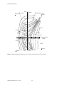
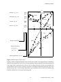
Four-Quadrant Head Curve for Semiscale Mod1 Pump (ANC-A-2083) .................48
Four-Quadrant Torque Curve for Semiscale Mod1 Pump (ANC-A-3449) ..............49
Homologous Head Curve..........................................................................................52
Homologous Torque Curve.......................................................................................53
Schematic of Mixing Junctions.................................................................................58
Jet Pump Model Design ............................................................................................60
Schematic Of Separator ............................................................................................64
Physical Picture of a Separator .................................................................................65
Separator Volume Fraction of Water Fluxed Out the Water Outlet ..........................66
Separator Volume Fraction Of Steam Fluxed Out The Steam Outlet .......................67
Schematic of a Cylindrical Accumulator..................................................................72
Schematic of a Spherical Accumulator.....................................................................73
Schematic of an Accumulator Showing Standpipe/Surgeline Inlet ..........................74
Possible Accumulator Configurations ......................................................................75
Mesh Point Layout....................................................................................................78
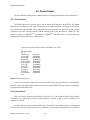
Input Data for a Power-Type General Table and Graph .........................................112
Example of Major Edit ...........................................................................................125
Example of Additional Output for Pumps, Turbines, and Accumulators...............132
Example of Reflood Major Edit..............................................................................139
Example of Cladding Oxidation and Rupture Major Edit ......................................140
Example of Radiation Major Edit ...........................................................................141
Example of Minor Edit ...........................................................................................142
Example of Printout Before the Diagnostic Edit When a Failure Occurs ..............144
Example of Printout Buried in the Diagnostic Edit When a Failure Occurs ..........145
Strip Input File ........................................................................................................146
vii
NUREG/CR-5535/Rev 1-Vol II
NUREG/CR-5535/Rev 1-Vol II
viii
TABLES
Page
2.1-1
2.1-2
2.3-1
2.4-1
2.4-2
4.1-1
4.1-2
4.1-3
4.2-1
8.3-1
Flow Regime Letters And Numbers .........................................................................14
Bubbly/Slug Flow Regime Numbers for Vertical Junctions.....................................15
Values of m, c7, and c8 for Tien’s CCFL Correlation Form .....................................31
Area Change Options................................................................................................39
Pump Homologous Curve Definitions......................................................................50
Logical Operations....................................................................................................87
Truth Table Examples ...............................................................................................89
Boolean Algebra Identities .......................................................................................90
Input Data for a Sample Problem to Test Pump, Generator, and Shaft ..................101
Flow Map Identifiers ..............................................................................................123
ix
NUREG/CR-5535/Rev 1-Vol II
NUREG/CR-5535/Rev 1-Vol II
x
INTRODUCTION
1 INTRODUCTION
The purpose of this volume is to help educate the code user by documenting the modeling experience
accumulated from developmental assessment and application of the RELAP5 code. This information
includes a blend of the model developers’ recommendations with respect to how the model is intended to
be applied and the application experience that indicates what has been found to work or not to work.
Where possible, approaches known to work are definitely recommended, and approaches known not to
work are pointed out as pitfalls to avoid.
1.1 General
The objective of the user’s guide is to reduce the uncertainty associated with user simulation of light
water reactor (LWR) systems. However, we do not imply that uncertainty can be eliminated or even
quantified in all cases, since the range of possible system configurations and transients that could occur is
large and constantly evolving. Hence, the effects of nodalization, time step selection, and modeling
approach are not completely quantified. As the assessment proceeds, there will be a continual need to
update the user guidelines document to reflect the current state of simulation knowledge.
1.2 Areas of Application
RELAP5 is a generic transient analysis code for thermal-hydraulic systems using a fluid that may be
a mixture of steam, water, noncondensables, and a nonvolatile solute.
The fluid and energy flow paths are approximated by one-dimensional stream tube and conduction
models. The code contains system component models applicable to LWRs. In particular, a point neutronics
model, pumps, turbines, generator, valves, separator, and controls are included. The code also contains a
jet pump component and an ecc mixer component.
The LWR applications for which the code is intended include accidents initiated from small break
loss-of-coolant accidents, operational transients such as anticipated transients without SCRAM, loss of
feed, loss-of-offsite power, and loss of flow transients. The reactor coolant system (RCS) behavior can be
simulated up to and slightly beyond the point of fuel damage.
1.3 Modeling Philosophy
RELAP5 is designed for use in analyzing system component interactions; it does not offer detailed
simulations of fluid flow within components. As such, it contains limited ability to model
multidimensional effects, either for fluid flow, heat transfer, or reactor kinetics. Exceptions are the
modeling of crossflow effects in a pressurized water reactor (PWR) core and the reflood modeling that
uses a two-dimensional conduction solution in the vicinity of a quench front. To further enhance the
overall system modeling capability, a control system model is included. This model provides a way to
perform basic mathematical operations, such as addition, multiplication, integration, and control
components such as proportional-integral, lag, and lead-lag controllers, for use with the basic fluid,
1
NUREG/CR-5535/Rev 1-Vol II
INTRODUCTION
thermal, and component variables calculated by the remainder of the code. This capability can be used to
construct models of system controls or components that can be described by algebraic and differential
equations. The code numerical solution includes the evaluation and numerical time advancement of the
control system coupled to the fluid and thermal system.
The hydrodynamic model and the associated numerical scheme are based on the use of fluid control
volumes and junctions to represent the spatial character of the flow. The control volumes can be viewed as
stream tubes having inlet and outlet junctions. The control volume has a direction associated with it that is
positive from the inlet to the outlet. Velocities are located at the junctions and are associated with mass and
energy flow between control volumes. Control volumes are connected in series, using junctions to
represent a flow path. All internal flow paths, such as recirculation flows, must be explicitly modeled in
this way since only single liquid and vapor velocities are represented at a junction. (In other words, a
countercurrent liquid-liquid flow cannot be represented by a single-junction.) For flows in pipes, there is
little confusion with respect to nodalization. However, in a steam generator having a separator and
recirculation flow paths, some experience is needed to select a nodalization that will give correct results
under all conditions of interest. Nodalization of branches or tees also requires more guidance.
Heat flow paths are also modeled in a one-dimensional sense, using a finite difference mesh to
calculate temperatures and heat flux vectors. The heat conductors can be connected to hydrodynamic
volumes to simulate a heat flow path normal to the fluid flow path. The heat conductor or heat structure is
thermally connected to the hydrodynamic volume through a heat flux that is calculated using heat transfer
correlations. Electrical or nuclear heating of the heat structure can also be modeled as either a surface heat
flux or as a volumetric heat source. The heat structures are used to simulate pipe walls, heater elements,
nuclear fuel pins, and heat exchanger surfaces.
A special, two-dimensional, heat conduction solution method with an automatic fine mesh rezoning
is used for low-pressure reflood. Both axial and radial conduction are modeled, and the axial mesh spacing
is refined as needed to resolve the axial thermal gradient. The hydrodynamic volume associated with the
heat structure is not rezoned, and a spatial boiling curve is constructed and used to establish the convection
heat transfer boundary condition. At present, this capability is specialized to the LWR core reflood
process, but the plan is to generalize this model to higher pressure situations so that it can be used to track
a quench front anywhere in the system.
The point reactor kinetics model is advanced in a serial and implicit manner after the heat
conduction-transfer and hydrodynamic advancements but before the control system advancement. The
kinetics model consists of a system of ordinary differential equations integrated using a modified RungeKutta technique. The integration time step is regulated by a truncation error control and may be less than
the hydrodynamic time step; however, the thermal and fluid boundary conditions are held fixed over each
hydrodynamic time interval. The reactivity feedback effects of fuel temperature, moderator temperature,
moderator density, and boron concentration in the moderator are evaluated, using averages over the
hydrodynamic control volumes and associated heat structures that represent the core. The averages are
weighted averages established a priori such that they represent the effect on total core power. Certain
NUREG/CR-5535/Rev 1-Vol II
2
INTRODUCTION
nonlinear or multidimensional effects caused by spatial variations of the feedback parameters cannot be
accounted for with such a model. Thus, the user must judge whether or not the model is a reasonable
approximation of the physical situation being modeled.
The control system model provides a way for simulating any lumped process, such as controls or
instrumentation, in which the process can be defined in terms of system variables through logical,
algebraic, differentiating, or integrating operations. These models do not have a spatial variable and are
integrated with respect to time. The control system is coupled to the thermal and hydrodynamic
components serially and implicitly. The control system advancement occurs after the heat conduction
transfer, hydrodynamic, and reactor kinetics advancements and uses the same time step as the
hydrodynamics so that new time thermal and hydrodynamic information is used in the control model
advancement. However, the control variables are fed back to the thermal and hydrodynamic model in the
succeeding time step, i.e., they are explicitly coupled.
A system code such as RELAP5 contains numerous approximations to the behavior of a real,
continuous system. These approximations are necessitated by the finite storage capability of computers, by
the need to obtain a calculated result in a reasonable amount of computer time, and in many cases because
of limited knowledge about the physical behavior of the components and processes modeled. For example,
knowledge is limited for components such as pumps and separators, processes such as two-phase flow, and
heat transfer. Examples of approximations required because of limited computer resources are limited
spatial nodalization for hydrodynamics, heat transfer, and kinetics; and density of thermodynamic and
property tables. In general, the accuracy effect of each of these factors is of the same order; thus,
improving one approximation without a corresponding increase in the others will not necessarily lead to a
corresponding increase in physical accuracy. At the present time, very little quantitative information is
available regarding the relative accuracies and their interactions. What is known has been established
through applications and comparison of simulation results to experimental data. Progress is being made in
this area as the code is used; but there is, and will be for some time, a need to continue the effort to quantify
the system simulation capabilities.
3
NUREG/CR-5535/Rev 1-Vol II
INTRODUCTION
NUREG/CR-5535/Rev 1-Vol II
4
HYDRODYNAMICS
2 HYDRODYNAMICS
The hydrodynamics simulation is based on a one-dimensional model of the transient flow for a
steam-water noncondensable mixture. The numerical solution scheme used results in a system
representation using control volumes connected by junctions. A physical system consisting of flow paths,
volumes, areas, etc., is simulated by constructing a network of control volumes connected by junctions.
The transformation of the physical system to a system of volumes and junctions is an inexact process, and
there is no substitute for experience. General guidelines have evolved though application work using
RELAP5. The purpose here is to summarize these guidelines.
In selecting a nodalization for hydrodynamics, the following general rules should be followed:
1.
2.
The length of volumes should be such that all have similar material Courant limits,
i.e., flow length divided by velocity about the same. (Expected velocities during the
transient must be considered.)
L
The volumes should have ---- ≥ 1 , except for special cases such as the bottom of a
D
L
pressurizer where a smaller ---- is desired to sharpen the emptying characteristic.
D
3.
The total system cannot exceed the computer resources. RELAP5 dynamically
allocates memory based on the requirements of each problem, and most models
require memory based on factors such as the number of volumes, junctions, number of
heat structures and the number of meshes, and the number and length of various userinput tables. The number of hydrodynamic volumes is a reasonable measure of
problem size, and typical LWR systems with over 600 volumes have been run on
workstations with 32 Mbytes of memory. The memory should be sufficiently large to
avoid paging during transient advancement.
4.
If possible, a nodalization sensitivity study should be made in order to estimate the
uncertainty owing to nodalization. Volume V provides guidance and examples of
appropriate nodalizations for reactor systems.
5.
Avoid nodalizations where a sharp density gradient coincides with a junction (a liquid
interface, for example) at steady-state or during most of the transient. This type of
situation can result in time-step reduction and increased computer cost.
6.
Eliminate minor flow paths that do not play a role in system behavior or are
insignificant compared to the accuracy of the system representation. This can not
usually be done until some preliminary trial calculations have been made that include
all the flow paths. Care must be used here because in certain situations flow through
minor flow paths can have a significant effect on system behavior. An example is the
effect of hot-to-cold-leg leakage on core level depression in a PWR under small break
loss-of-coolant accident conditions.
5
NUREG/CR-5535/Rev 1-Vol II
HYDRODYNAMICS
7.
Establish the flow and pressure boundaries of the system beyond which modeling is
not required and specify appropriate boundary conditions at these locations.
2.1 Basic Flow Model
The RELAP5 flow model is a nonhomogeneous, nonequilibrium two-phase flow model. See Section
3 of Volume I for a detailed description of the model and the governing equations. Options exist for
homogeneous, equilibrium, or frictionless models if desired. These options are included to facilitate
comparisons with other homogeneous and/or equilibrium codes. Generally, the code will not run faster if
these options are selected.
The RELAP5 flow model is a one-dimensional, stream-tube formulation in which the bulk flow
properties are assumed to be uniform over the fluid passage cross-section. The control volumes are finite
increments of the flow passage and may have a junction at the inlet or outlet (normal junctions) or at the
side of a volume (crossflow junctions). The stream-wise variation of the fluid passage is specified through
the volume cross-sectional area, the junction areas, and through use of the smooth or abrupt area change
options at the junctions. The smooth or abrupt area change option affects the way in which the flow is
modeled, both through the calculation of loss factors at the junction and through the method used to
calculate the volume average velocity. (Volume average velocity enters into momentum flux, boiling heat
transfer, and wall friction calculations.) The abrupt area change model should be used to model the effect
of sudden area changes such as reducers, orifices, or any obstruction in which the flow area variation with
length is great enough to cause turbulence and flow separation. Only flow passages having a low wall
angle (< 10 degrees, including angle) should be considered smooth. An exception to this rule is the case
where the user specifies the kinetic loss factor at a junction and uses the smooth option. This type of
modeling should only be attempted for cases where the actual flow area change is modest (less than a
factor of two).
The hydrodynamic boundaries of a system are modeled using time-dependent volumes and junctions.
For example, a reservoir condition would normally be modeled as a constant pressure source of mass and
energy (a sink in the case of an outflow boundary). The reservoir is connected to the system through a
normal junction, and the inflow velocity is determined from the momentum equation solution. For this type
of boundary, some caution is required, since the energy boundary condition is in terms of the thermal
energy rather than total energy. Thus, as the velocity increases, the total energy inflow increases owing to
the increase in kinetic energy. This effect can be minimized for simulation of a reservoir by making the
cross-sectional area of the time-dependent volume very large compared to the inlet junction area. This
policy should be followed for outflow boundaries as well, or else flow reversals may occur.
A second way of specifying a flow boundary is using the time-dependent junction in addition to a
time-dependent volume. This type of boundary condition is analogous to a positive displacement pump
where the inflow rate is independent of the system pressure. In this case, the cross-sectional area of the
time-dependent volume is not used because the velocity is fixed and the time-dependent volume is only
used to specify the properties of the inflow. Thus, the total energy of the inflow is specified. When only
time-dependent junctions are used as boundary conditions, the system pressure entirely depends on the
NUREG/CR-5535/Rev 1-Vol II
6
HYDRODYNAMICS
system mass, and, in the case of all liquid systems, a very stiff system results. An additional fact that
should be considered when using a time-dependent junction as a boundary is that pump work is required
for system inflow if the system pressure is greater than the time-dependent volume pressure. In particular,
any energy dissipation associated with a real pumping process is not simulated. The flow work done
against the system pressure is approximated by work terms in the thermal energy equation.
In RELAP5, any volume that does not have a connecting junction at an inlet or outlet is treated as a
closed end. Thus, no special boundary conditions are required to simulate a closed end.
The fluid properties at an outflow boundary are not used unless flow reversal occurs. In this respect,
some caution is necessary and is best illustrated by an example. In the modeling of a subatmospheric
pressure containment, saturated steam is often specified for the containment volume condition. This will
result in the outflow volume containing pure steam at low pressure and temperature. If in the course of
calculation a flow reversal occurs, even a very minute one (possibly caused by numerical noise), a
cascading result occurs. The low-pressure or low-temperature steam can rush into a volume at higher
pressure and rapidly condense. The rapid condensation leads to depressurization of the volume and
increased flow. Such a result can be avoided by using air or superheated steam in the containment volume.
A general guide to modeling hydrodynamic boundary conditions is to simulate the actual process as
closely as possible. This guideline should be followed unless initial calculations result in unphysical results
because of unanticipated numerical idiosyncrasies.
Only the algebraic sign is needed in the one-dimensional hydrodynamic components to indicate the
direction of vector quantities, i.e., the volume and junction velocities. Both the volumes and the junctions
have coordinate directions that are specified through input. Each hydrodynamic volume has three
coordinate directions, named x, y, and z, and each coordinate direction has an associated inlet and outlet
face. The coordinate direction is positive from the inlet to the outlet. The normal, one-dimensional flow is
along the x-coordinate. Normal volume connections are to the inlet and outlet faces associated with the xcoordinate. Crossflow connections are to the inlet and outlet faces associated with coordinates orthogonal
to the x-coordinate, that is, the y- and z-coordinates.
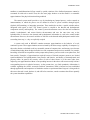
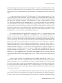
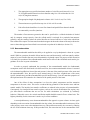
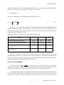
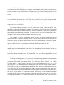
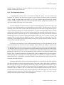
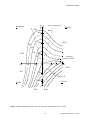
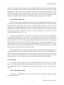
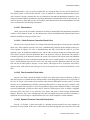
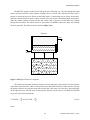
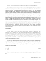
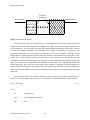
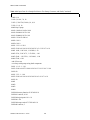
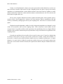
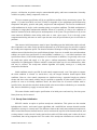
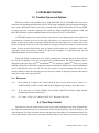
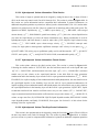
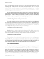
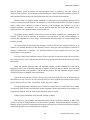
Which faces of a volume are the inlet or outlet faces depend upon the specifications of the volume
orientation. For a positive vertical elevation change, the inlet is at the lowest elevation, whereas for a
negative vertical elevation change, the inlet is at the highest elevation of the volume. For a horizontal
volume, whether the inlet is at the left or right depends upon the azimuthal angle. (A zero value implies an
orientation with the inlet at the left.) This orientation of a horizontal volume is not important as far as
hydrodynamic calculations are concerned but is important if one tries to construct a three-dimensional
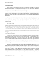
picture of the flow path. Several possible volume orientations, depending upon the input values for the
azimuthal and inclination angles, are illustrated in Figure 2.1-1.
The junction coordinate direction is established through input of the junction connection code (e.g.,
Words W1 and W2 of Cards CCC0101 through CCC0109, Section A-7.4 of Appendix A for a single-
7
NUREG/CR-5535/Rev 1-Vol II
HYDRODYNAMICS
0
i
i
0
azimuthal angle = 0 or 360
inclination angle = 0
azimuthal angle = 180
inclination angle = 0
0
0
i
i
azimuthal angle = 180
inclination angle = 45
azimuthal angle = 0 or 360
inclination angle = 45
i
0
i
0
azimuthal angle = 0 or 360
inclination angle = -45
azimuthal angle = 0 or 360
inclination angle = 45
0
i
0
i
azimuthal angle = 0 to 360
inclination angle = 90
azimuthal angle = 0 to 360
inclination angle = -90
Figure 2.1-1 Possible Volume Orientation Specifications
NUREG/CR-5535/Rev 1-Vol II
8
HYDRODYNAMICS
junction component). The junction connection codes designate a from and a to component, and the velocity
is positive in the direction from the from component to the to component. The connection codes can be
entered in an old or an expanded format. The expanded format is recommended, but the old format is still
valid.
A connection code has the format CCCVV000N, where CCC is the component number, VV is the
volume number, and N is the face number, where zero indicates the old format and nonzero indicates the
expanded format. The old format (N = 0) can only specify connections to the faces associated with normal
flow, that is, flow along the x-coordinate. In the old format, VV is not a volume number but, instead,
VV = 00 specifies the inlet face of the component, and VV = 01 specifies the outlet face of the component.
The volume number is only implied. For components specifying single-volumes (currently only a pipe
specifies multiple volumes), normal flow (as opposed to crossflow) to either the inlet or outlet face can be
specified. For a pipe, however, the old format allows specification of normal flow only to the inlet of the
first pipe volume or to the outlet of the last pipe volume. Crossflow meaning connections to faces
associated with y- or z-faces cannot be specified with the old format.
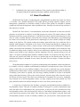
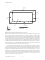
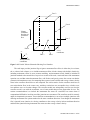
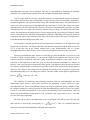
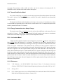
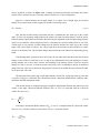
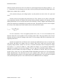
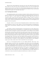
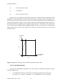
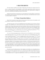
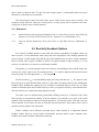
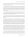
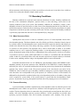
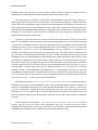
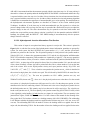
The expanded connection code assumes that a volume has six faces, i.e., an inlet and outlet for each
of three coordinate directions (see Figure 2.1-2 and Figure 2.1-3). The expanded connection code
indicates the volume being connected and through which face it is being connected. In the new format (N
nonzero), N is the face number and VV is the volume number. For components specifying single-volumes,
VV is 01; but for pipes, VV can vary from 01 for the first pipe volume to the last pipe volume number. The
quantity N is 1 and 2 for the inlet and outlet faces, respectively, for the volume’s normal or x-coordinate
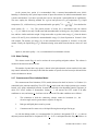
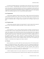
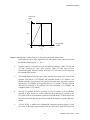
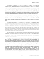
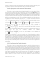
direction. The quantity N is 3 and 4 to indicate inlet and outlet faces, respectively, for the volume’s ycoordinate direction, and N is 5 and 6 to indicate inlet and outlet faces, respectively, for the volume’s zcoordinate direction. Entering N as 1 or 2 specifies normal connections to a volume; entering N as 3
through 6 specifies a crossflow connection to a volume. In Figure 2.1-2 and Figure 2.1-3, the world
(inertial) coordinates are indicated by xo, yo, and zo, whereas the local coordinates for the volume are
indicated by x, y, and z. Figure 2.1-2 is for a horizontal volume. Figure 2.1-3 is for a vertical volume, and
is obtained from the horizontal volume (Figure 2.1-2) by a 90o counter-clockwise rotation about the local
y-axis.
Average volume velocities are computed along each coordinate direction that is active. The xcoordinate is assumed active, and a warning message is issued during input processing if no junctions
attach to normal faces. A y- or z-coordinate is active only if a junction attaches to one of the associated
faces. The average volume velocity for each coordinate direction involves only junction velocities at the
faces associated with that coordinate direction. Thus, a crossflow entering a y-face does not contribute to
the computation of the volume velocity in the x-direction. But that crossflow does contribute to the average
velocity in the y-direction.
Users of previous versions of RELAP5 will note that the crossflow discussed above is different from
older versions. The crossflow capability has been improved, but unfortunately the differing meanings for
the term crossflow may lead to misunderstanding. The previous use of crossflow implied the following:
9
NUREG/CR-5535/Rev 1-Vol II
HYDRODYNAMICS
Face 6
Face 4
Face 2
Face 1
z
y
x
Face 5
Face 3
zo
yo
xo
World (inertial)
coordinates
Volume coordinate direction (x)
for normal flow
Figure 2.1-2 Horizontal Volume Schematic Showing Face Numbers
Flow entered a face orthogonal to the normal flow; crossflows never contributed to any average volume
velocity; a limited form of the momentum equation was used; and face numbers 3 through 6 and/or
junction flags could specify a crossflow connection. The limited momentum equation ignored momentum
flux, wall friction, and gravity terms. Now, crossflow means only that the connection is to a face other than
one of the normal faces. Note especially that crossflow does not imply a modified form of the momentum
equation. The same momentum equation options are available to both normal flows and crossflows. The
standard one-dimensional momentum equations can be applied to both normal and crossflows. Optionally,
and only through the use of the momentum flux junctions flags, the momentum flux contribution in the
from or to volume can be ignored for normal and crossflow connections.
There is no difference in the application of the conservation equations to the normal and crossflow
types of connections. The only difference is that the term normal is applied to the flow that would occur in
a strictly one-dimensional volume; crossflow is an approximation to multidimensional effects consisting of
applying the one-dimensional momentum equation to each of the coordinate directions in use. To give
some perspective to the approximation, the three-dimensional momentum equation contains nine terms for
momentum flux; the momentum in each of the three directions being convected by velocities in the three
directions. In the crossflow model, only three momentum flux terms are used--the momentum in each
direction convected by velocity in the same direction.
NUREG/CR-5535/Rev 1-Vol II
10
HYDRODYNAMICS
Face 2
Face 4
Volume
coordinate
direction (x)
for normal
flow
Face 5
x
y
Face 6
z
zo
yo
Face 3
Local
coordinates
Face 1
xo
World (inertial)
coordinates
Figure 2.1-3 Vertical Volume Schematic Showing Face Numbers
The code input provides junction flags to ignore momentum flux effects in either the from volume,
the to volume, both volumes, or to include momentum effects in both volumes (the default). Intuitively,
including momentum effects is more accurate modeling, and momentum effects should be included in
junctions attached to the normal faces. In previous versions of the code, a restricted form of the momentum
equation was used that omitted momentum flux, wall friction, and gravity terms. One reason was that the
geometric information necessary for computing these terms was not available and average volume velocity
terms in the crossflow directions were not computed. The earliest motive for the crossflow model was to
treat recirculation flows in the reactor core, and these restrictions were acceptable since velocities were
low and there were no elevation changes. The crossflow model was subsequently used for tees since the
crossflow model, even with the restrictions, was a better model than previous approaches for tees. The
current recommendation is to include the momentum flux terms for crossflows but remove them if
computational difficulties involving crossflow junctions are encountered. The crossflow model is currently
under developmental assessment. A more definite recommendation is not to have multiple junctions with
differing momentum flux options attached to the same coordinate direction. Even though the momentum
flux is ignored in one junction, its velocity contributes to the average velocity in that coordinate direction
and thus other junctions using momentum flux terms use that average volume velocity.
11
NUREG/CR-5535/Rev 1-Vol II
HYDRODYNAMICS
The current crossflow model requires input information for the y- and z-coordinates similar to that
entered for the x-coordinate. Default data for the y and z-coordinates are obtained from the x-coordinate
data by assuming the volume is a section of a right circular pipe. Optional input data may be entered when
this assumption is not valid.
In major edits and similar input edits, the junction connection code is edited in the new format. Note
that the new logic allows branching and merging flow (i.e., multiple junctions at a face) at any volume,
including interior pipe volumes. The primary reason for this change is to permit crossflow to all volumes in
a pipe. Now it is possible to use pipe volumes to represent axial levels in a vessel and to use multiple pipe
components to represent radial or azimuthal dependence. Single-junctions can crosslink any of the pipe
volumes at the same axial level.
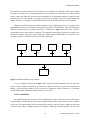
A simpler method to crosslink volumes is to use the multiple junction component. This component
describes one or more junctions, with the limitation that all volumes connected by the junctions must be
part of the same hydrodynamic system. Although this component can be considered a collection of singlejunctions, its common use is to crosslink adjacent volumes of parallel pipes. Because the junctions linking
pipe volumes tend to be similar, N junctions crosslinking N volumes per pipe can be entered with the
amount of input comparable to one junction.
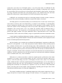
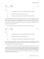
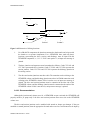
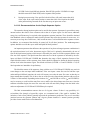
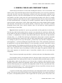
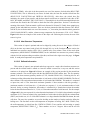
A sketch showing a series of three horizontal volumes connected by two junctions is shown in
Figure 2.1-4 to illustrate some of the possible coordinate orientations that result from combinations of the
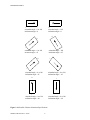
connection codes and the volume orientation data. In Figure 2.1-5, two possible combinations are
illustrated for the connection of two vertical volumes. Figure 2.1-5a shows the two volumes unconnected;
Figure 2.1-5b shows the result when the outlet of Volume 1 is joined to the inlet of Volume 2; and Figure
2.1-5c shows the result when the inlet of Volume 1 is connected to the inlet of Volume 2. In particular,
note that the geometry can be modified from a straight passage to a manometer configuration by simply
reversing the inlet/outlet designator in the junction connection code.
i
i
0
0
0
i
Figure 2.1-4 Sketch of Possible Coordinate Orientation for Three Volumes and Two Junctions
When systems of volumes or components are connected in a closed loop, the summation of the
volume elevations must close when they are summed according to the junction connection codes and
sequence, or an unbalanced gravitational force will result. RELAP5 has an input processing feature that
finds all loops or closed systems (which are defined by the input) and checks for elevation closure around
NUREG/CR-5535/Rev 1-Vol II
12
HYDRODYNAMICS
1
2
a
2
1
b
2
1
c
Figure 2.1-5 Sketch of Possible Vertical Volume Connections
each loop. The error criterion is 10-4 m. If closure is not obtained, the fail flag is set, and no transient or
steady-state calculations will be made. The elevation checker will print out that elevation closure does not
occur at a particular junction that formed a closed loop during input processing. The junction at which
closure of the loop occurs is somewhat arbitrary and depends on the input order of the components.
The elevation checking with crossflows differs from earlier versions of RELAP5. The elevation
checking starts from the center of a volume with the initial volume and its elevation obtained from input
data or defaulted. Using to and from junction information and elevation change information from the
connected volumes, the elevation to the common face of the volumes is computed; then, the elevation of
the center of the connected volume is computed. This computing of the elevations by tracking the junctions
continues until all junctions have been used. Whenever a volume is reentered, the newly obtained elevation
is compared to the previously computed elevation, and an error occurs if they do not match. With the
previous crossflow model, the elevation from the center to a face was zero for a crossflow connection. This
meant that the same elevation would be obtained regardless of which face the crossflow connection used.
The face number is now important, both for elevation checking and in computing elevation effects,
momentum flux effects, and friction. We recommend that decks prepared for previous versions of the code
have all crossflow connections reviewed for use with the newer crossflow model.
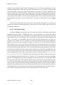
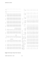
The junctions are printed out in the major edits in the hydrodynamic junction information sections
(Section 8.3.2.9 and Section 8.3.2.10). The from and to volumes are listed for each junction. In addition,
the flow regimes for the volumes (floreg) and the junctions (florgj) are also listed using three letters. It is
13
NUREG/CR-5535/Rev 1-Vol II
HYDRODYNAMICS
also possible to list the flow regime for the volumes and the junctions in the minor edits and plots, where a
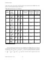
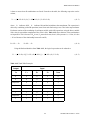
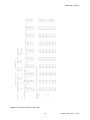
number is used. Table 2.1-1 shows the three-letter code and number used for each flow regime.
Table 2.1-1 Flow Regime Letters And Numbers
Flow regime
Three-letter code
(major edits)
Number
(minor edits/plots)
High mixing bubbly
CTB
1
High mixing bubbly/mist transition
CTT
2
High mixing mist
CTM
3
Bubbly
BBY
4
Slug
SLG
5
Annular mist
ANM
6
Mist pre-CHF
MPR
7
Inverted annular
IAN
8
Inverted slug
ISL
9
Mist
MST
10
Mist post-CHF
MPO
11
Horizontal stratified
HST
12
Vertical stratified
VST
13
Level tracking
LEV
14
Jet junction
JET
15
ECC mixer wavy
MWY
16
ECC mixer wavy/annular mist
MWA
17
ECC mixer annular mist
MAM
18
ECC mixer mist
MMS
19
ECC mixer wavy/slug transition
MWS
20
ECC mixer wavy-plug-slug transition
MWP
21
ECC mixer plug
MPL
22
ECC mixer plug-slug transition
MPS
23
ECC mixer slug
MSL
24
NUREG/CR-5535/Rev 1-Vol II
14
HYDRODYNAMICS
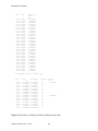
Table 2.1-1 Flow Regime Letters And Numbers (Continued)
Flow regime
Three-letter code
(major edits)
Number
(minor edits/plots)
ECC mixer plug-bubbly transition
MPB
25
ECC mixer bubbly
MBB
26
Table 2.1-2 Bubbly/Slug Flow Regime Numbers for Vertical Junctions
Geometry and flow conditions
Correlations used
Numbers
(minor edits/plots)
Rod bundles
EPRI
2
High up/down flows in small pipes
EPRI
3
Zuber-Findlay slug
4
EPRI & Zuber-Findlay slug
5
EPRI
9
Low up/down countercurrent flows in
intermediate pipes
Churn-turbulent bubbly
10
Transition regions between 10 and 12
Churn-turbulent bubbly &
Kataoka-Ishii
11
Low up/down countercurrent flows in
intermediate pipes
Kataoka-Ishii
12
Transition between regions 9 and 10-11-12
EPRI & Churn-turbulent
bubbly/Kataoka-Ishii
13
Large pipes
Churn-turbulent bubbly
14
Churn-turbulent bubbly &
Kataoka-Ishii
15
Kataoka-Ishii
16
Low up/down countercurrent flows in small
pipes
Transition regions between 3 and 4
High up/down flows in intermediate pipes
Transition regions between 14 and 16
Large pipes
In the bubbly and slug flow regimes for vertical junctions, it is possible to list an additional flow
regime number (iregj) in the minor edits and plots that is associated with a particular geometry/flow and
correlation that is used in the interphase drag. If not in bubbly or slug flow and not a vertical function, the
number will be zero. Table 2.1-2 shows the number used for each regime. In the transition regions (11 and
15), a fraction is added to the number (between 0 and 1) that indicates how far the junction conditions are
15
NUREG/CR-5535/Rev 1-Vol II
HYDRODYNAMICS
between churn-turbulent bubbly and Kataoka-Ishii, based on the dimensionless vapor superficial velocity
( jg ) .
+
The interphase friction model for bundles (i.e., core and steam generator) can be activated with a
volume control flag (b). The model is based on a correlation from EPRI, as discussed in Volume I of this
manual. When in bubbly or slug flow, the flow regime number is 2, as indicated in Table 2.1-2; otherwise
it is 0.
The user should be aware that all plant or experimental facility geometries that are not circular
should have an input junction hydraulic diameter to specify the necessary information required for the code
calculated interphase friction. For bundles and steam generators, the junction hydraulic diameter should
match the volume hydraulic diameter (including grid spacers, which should use the volume hydraulic
diameter at the junction). In addition for grid spacers, the volume flow area should be used at the junction
and the user-input loss should be multiplied by ratio of squared areas of the volume and the grid spacer.
For area changes, the donor diameter for the normal flow direction is recommended. For orifices, the
actual diameter is recommended.
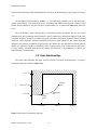
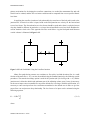
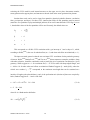
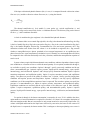
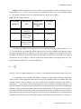
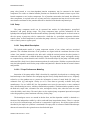
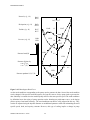
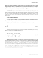
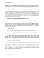
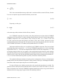
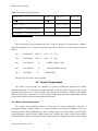
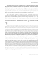
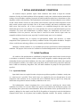
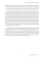
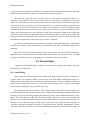
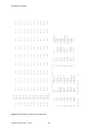
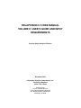
2.2 State Relationships
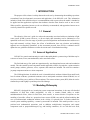
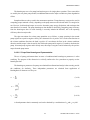
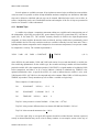
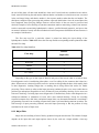
The steam table subroutine has upper and lower limits on pressure and temperature. A pressuretemperature diagram is shown in Figure 2.2-1.
1 x 10⁸ Pa
P
Critical
point
2.212 x 10⁷ Pa
Saturation
line
611.2 Pa
Triple
point
0
273.16 K
647.3 K
T
Figure 2.2-1 Pressure-Temperature Diagram
NUREG/CR-5535/Rev 1-Vol II
16
5,000 K
HYDRODYNAMICS
If the calculation predicts a pressure and temperature in the shaded region, a water property error will
result, and the code will cut the time step. If the calculation continues to predict pressure and temperature
in the shaded region down to the minimum time step, the calculation will be terminated.
2.3 Process Models
In RELAP5, process models are used for simulation of processes that involve large spatial gradients
or which are sufficiently complex that empirical models are required. The flow processes for an abrupt
area change, a choked flow, a branch, reflood, noncondensables, water packer, CCFL, level tracking, and
thermal stratification are all simulated using specialized modeling. These particular processes are not
peculiar to a component and will be discussed as a group. Some components, such as pumps and
separators, also involve special process models; these models will be discussed with the component
models. The use of the process models is specified through input, and proper application is the
responsibility of the user. Under certain circumstances, we recommend that the user not mix process
models; e.g., we recommend the user not use the choking model at a junction connected to either the side
of a volume where the abrupt area change is activated for the junction and more than one junction is
connected. The purpose of this section is to advise the user regarding proper application of the process
models.
2.3.1 Abrupt Area Change
The abrupt area change option should generally be used in the following situations:
1.
Sharp edged area changes.
2.
Manifolds and plena connecting parallel flow passages.
3.
At break locations.
For the abrupt area model, the junction area (upon which the velocities are based) is the minimum
area of the two connecting volumes. The abrupt area change model is discussed in more detail in Section
2.4.1.
In addition to the computed form loss from the abrupt area change model, users have the option of
input form loss factors to achieve the desired pressure drop. See Section 2.3.3.3 for discussion for
modeling of minor flow paths. It is recommended that the abrupt area change model not be used in
situations where the area change ratio is greater than 10. For this situation, the smooth area change option
and an appropriate loss coefficient is recommended.
The pressure drop calculated by using form losses is a function of junction velocity.
17
NUREG/CR-5535/Rev 1-Vol II
HYDRODYNAMICS
2.3.2 Choked Flow
The choked flow option is specified in the junction flags on the junction geometry card. In general,
the choked flow model should be used at all exit junctions of a system. We recommend that the choked
flow model be usually used at the choke plane and that the user not model anything past this plane.
(Therefore, just use a time-dependent volume downstream of the choke plane.) Internal choking is allowed
but may not be desirable under certain conditions. Some applications of RELAP5 require that volumes
downstream of the choke plane be modeled with non-time-dependent volumes. For this case, the user
should monitor the mass error in the downstream volumes to ensure that the total mass error is not
governed by these volumes. This is done by examining the hydrodynamic time step control information in
the major edits (see Section 8.3.2); one of columns labeled LRGST.MASS ERR gives the number of times
a volume had the largest mass error. If the mass error in these volumes is large (i.e., the number of times a
volume had the largest mass error is high), the user should consider adjusting the size of the volumes. This
would involve reducing the size of these volumes, since the mass error is given by the density error times
the volume.
The recommended input junction flags when the choking model is on (c = 0) are abrupt (a = 1 or 2)
and nonhomogeneous (h = 0). (1) With regard to the abrupt area options (a = 1 or 2), these are discussed in
Section 2.4.1. The full abrupt area change model (a = 1, code calculated losses) is recommended for
sudden (i.e., sharp, blunt) area changes, while the partial abrupt area change model (a = 2, no code
calculated losses, user input losses are to be used) is recommended for rounded or beveled area changes.
The extra interphase drag term (see Volume IV) in the abrupt area model (a = 1 or 2), helps ensure more
homogeneous flow that would be expected through a sudden area change. The smooth area change option
(a = 0) is recommended only for when there is no area changes or there are smooth area changes (i.e.,
venturi). (2) With regard to the nonhomogeneous (h = 0) option, it is generally recommended that h = 0 be
used. There may be rare situations where the combined interphase drag is too low, resulting in too much
slip and too low mass flow. For this situation, the homogeneous option (h = 1 or 2) is recommended. (3)
The user should monitor the calculated results for nonphysical choking. If this occurs, the user should turn
choking off (c = 1) at junctions where this occurs.
Guidelines for the discharge coefficients (subcooled and two-phase) are as follows. For a break
nozzle/venturi geometry, a discharge coefficient of nearly 1.0 should be used. For an orifice geometry, the
discharge coefficient depends on the break configuration and may be somewhat less than 1.0.
dA
The throat ------- used in subcooled choking, which is denoted by
dx
dA
------- in Volume I of this manual,
dx t
is calculated differently for the normal junction abrupt area option and the normal junction smooth area
option.
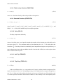
For the recommended abrupt area change option, the following formula is used:
NUREG/CR-5535/Rev 1-Vol II
18
HYDRODYNAMICS
AK – At
dA
-------
= ----------------- dx t, abrupt
10.0D K
(2.3-1)
where
AK
=
the upstream volume flow area in the coordinate direction of the junction
At
=
the throat or junction area (minimum physical area)
DK
=
the upstream volume diameter in the coordinate direction of the junction.
It is recommended the user input the actual physical values for AK, At, and DK. This formula is empirical,
and the data base is limited. It was developed primarily to obtain the proper subcooled discharge at the
break for the LOFT-Wyle Blowdown Test WSB03R,2.3-1 which is one of the developmental assessment
separate-effects test problems. In addition, it has been used successfully in many Semiscale test
comparisons for the break flow.2.3-2
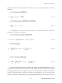
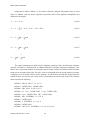
If the user selects the smooth area change option, the code uses the following formula:
A K – At
dA
-------
= ----------------- dx t, smooth
0.5∆x K
(2.3-2)
where
AK
=
the upstream volume flow area in the coordinate direction of the junction
At
=
the throat or junction area (minimum physical area)
∆x K
=
is the upstream volume length in the coordinate direction of the junction.
The smooth area option is intended to be used for smoothly varying geometries. The length 0.5 ∆xK would
be the actual length of the upstream volume (AK) to the throat (At). Since the smooth area change option is
not recommended, this formula has had little assessment.
Sometimes, it is observed that the choking junction oscillates in time between the inlet and outlet
junctions of a control volume. This may induce flow oscillations and should be avoided. The situation most
often occurs in modeling a break nozzle. The choking plane is normally located in the neighborhood of the
throat. The break can be adequately modeled by putting the break junction at the throat and including only
the upstream portion of the nozzle. If the entire nozzle is modeled, the choked flow option should be
applied only to the junction at the throat.
19
NUREG/CR-5535/Rev 1-Vol II
HYDRODYNAMICS
The internal choking option must be removed when supersonic flows are anticipated or when its
application causes unphysical flow oscillations. Typical cases are propagation of shock waves downstream
from a choked junction. Sometimes, it is necessary to remove the choking option at junctions near a known
internal choked junction in order to avoid oscillations.
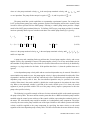
2.3.3 Branching
A fundamental and vital model needed for simulation of fluid networks is the branched flow path.
Two types of branches are common, the tee and the plenum. The tee involves a modest change in flow area
from branch to branch and a large change in flow direction, while the plenum may involve a very large
change in flow area from branch to branch and little or no change in flow direction. In PWR simulations, a
tee model would be used at pressurizer surge line connections, hot leg vessel connections, and cold leg
connections to the vessel inlet annulus. A plenum model would be used for modeling upper and lower
reactor vessel plenums, steam generator models, and low-angle wyes.
Two special modeling options are available for modeling branched flow paths. These are a crossflow
junction model and a flow stratification model, in which the smaller pipe at a tee or plenum may be
specified as connected to the top, center, or bottom of a larger connecting pipe. When stratified flow is
predicted to exist at such a branch, vapor pullthrough and/or liquid entrainment models are used to predict
the void fraction of the branched flow. The use of these models for simulating tees, plenums, and leak
paths are discussed in greater detail below.
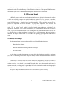
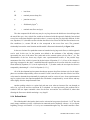
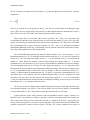
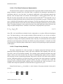
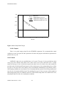
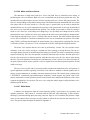
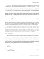
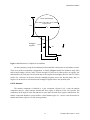
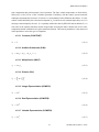
2.3.3.1 Tees.
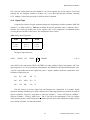
The simplest tee is the 90-degree tee, in which all branches have the same or comparable diameters.
The recommended nodalization for this flow process is illustrated in Figure 2.3-1. The small volume at the
intersection of the side branch with the main flow path should have a length equal to the pipe diameters.
Generally, this length will be shorter than most other hydraulic volumes and will have a relatively small
material Courant limit. The code, however, has a time step scheme that permits violation of the material
Courant for an isolated volume for the semi-implicit scheme. Thus, this modeling practice may not result
in a time step restriction. User experience has shown that if the code runs too slowly and is Courant-limited
in the small volume, it is possible to increase the length of the volume to allow faster running without
adversely affecting the results.
The Junction J3 is specified as a half normal junction and half crossflow junction. The half of
Junction J3 associated with Volume V4 is a normal junction, whereas the half associated with Volume V2
is a crossflow junction. The junction specification is made using the junction flag efvcahs, which (for a
single-junction) is Word W6(I) of Cards ccc0101 through ccc0109. As noted in previous crossflow
discussions, the same momentum equation options are used available in both normal and crossflow. Both
flow types allow ignoring of momentum flux and wall friction terms through the use of volume and
junction flags. User experience shows that temperature oscillations may develop in Volume V2. It may be
necessary to increase the length of Volume V2 to remove the oscillations. In general, a user loss coefficient
will be needed at Junction J3. This coefficient should be determined to obtain the proper pressure drop.
NUREG/CR-5535/Rev 1-Vol II
20
HYDRODYNAMICS
V4
J3
V1
J1
J2
V2
V3
Figure 2.3-1 A 90-Degree Tee Model Using a Crossflow Junction
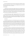
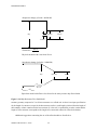
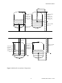
A tee can also be modeled using the branch component, as illustrated in Figure 2.3-2. This approach
has the advantage that fewer volumes are used. Disadvantages are that the calculated result may be altered,
depending on whether Junction J2 is connected to Volume V1 or V2, and that the flow division has less
resolution at the tee in the presence of sharp density gradients. In cases where the Volumes V1 and V3 are
nearly parallel, the model illustrated in Figure 2.3-2 may be a more accurate representation of the physical
process (such as for a wye).
V3
J2
V1
V2
J1
Branch
Figure 2.3-2 Tee Model Using a Branch Component
21
NUREG/CR-5535/Rev 1-Vol II
HYDRODYNAMICS
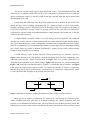
2.3.3.2 Branch.
The branch model approximates the flow process that occurs at merging or dividing flows, such as at
wyes and plenums. This model does not include momentum transfer caused by mixing and thus is not
suited for high-velocity merging flows. A special component, the JETMIXER, is provided for modeling
the mixing of high-velocity, parallel streams. Application of this model is discussed in Section 2.4.9.
A branch component consists of one system volume and zero to nine junctions. The limit of nine
junctions is due to a card numbering constraint. Junctions from other components, such as single-junctions,
pumps, other branches, or even time-dependent junction components, may be connected to the branch
component. The results are identical whether junctions are attached to the branch volume as part of the
branch component or as part of other components. Use of junctions connected to the branch but defined in
other components is required in the case of pump and valve components. Any of these may also be used to
attach more than the maximum of nine junctions that can be described in the branch component input.
A typical one-dimensional branch is illustrated in Figure 2.3-3. The figure is only one example and
implies merging flow. Additional junctions could be attached to both ends, and any of the volume and
junction coordinate directions could be changed. The actual flows may be in any direction; thus, flow out
of Volume V3 through Junction J1 and into Volume V3 through Junction J2 is permitted.
V1
J1
AJ1,V3
(vf)
V3 J3
V4
V3
V2
J2
(vg)
AJ2,V3
V3
Figure 2.3-3 Typical Branching Junctions
The volume velocities are calculated by a method that averages the phasic mass flows over the
volume cell inlets and outlets. The volume velocities of Volume V3 are used to evaluate the momentum
flux terms for all junctions connected to Volume V3. The losses associated with these junctions are
calculated using a stream tube formulation based on the assumption that the fraction of volume flow area
NUREG/CR-5535/Rev 1-Vol II
22
HYDRODYNAMICS
associated with a junction stream tube is the same as the volumetric flow fraction for the junction within
the respective volume. Also, using the junction flow area, the adjacent volume flow areas, and the branch
volume stream tube flow area, the stream tube formulation of the momentum equation is applied at each
junction. However, if the smooth area change is specified, large changes in flow can lead to nonphysical
results. Therefore, it is normally recommended that the abrupt area change option be used at branches.
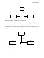
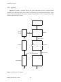
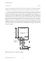
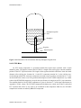
Plenums are modeled using the branch component. Typical LWR applications of a plenum are the
upper and lower reactor vessel regions, steam generator plenums, and steam domes. The use of a branch to
model a plenum having four parallel connections is illustrated in Figure 2.3-4. The flows in such a
configuration can be either inflows or outflows. The junctions connecting the separate flow paths to the
plenum are ordinary junctions with the abrupt area change option recommended. It is possible to use
crossflow junctions at a branch for some or all of the connections.
J1
V4
V3
V2
V1
J2
J3
J4
V5
J5
V6
Figure 2.3-4 Plenum Model Using a Branch
A wye is modeled, as illustrated in Figure 2.3-3, using the branch component. The flow can either
merge or divide. Either the smooth or the abrupt area change option may be used. If the smooth area
change is specified, large changes in flow can lead to nonphysical results. Therefore, it is normally
recommended that the abrupt area change option be used at wyes.
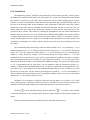
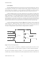
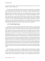
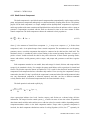
2.3.3.3 Leak Paths.
An application, that may or may not involve branching but which is frequently a source of problems,
is the modeling of small leak paths. These may be high-resistance paths or may involve extreme variations
in flow area. The approximation of the momentum flux terms for such flow paths is highly uncertain and
can lead to large forces, resulting in numerical oscillations. Modeling of small leak paths was one of the
23
NUREG/CR-5535/Rev 1-Vol II
HYDRODYNAMICS
primary motivations for developing the crossflow connections. As needed, the momentum flux and wall
friction can be omitted, and the flow resistance could instead be computed from a user-specified kinetic
loss factor.
In applying the crossflow junction to leak path models, the actual area of the leak path is used as the
junction area. A kinetic loss factor is input, based on the fluid junction area velocity for the forward and
reverse loss factors. The forward and reverse loss factors should be equal unless there is a physical reason
why they should be different. In particular, a very large forward and small reverse loss factor should not be
used to simulate a check valve. This approach can cause code failure. A typical leak path model between
vertical volumes is illustrated in Figure 2.3-5.
V2
V1
Figure 2.3-5 Leak Path Model Using the Crossflow Junction
Minor flow paths having extreme area variations or flow splits, in which the minor flow is a small
fraction of the main flow (< 0.1), can also be modeled using the standard junction by the following special
procedures. The smooth area change option is used for the junction (the efvcahs flag with a = 0), and the
junction area is allowed to default (the minimum area of the adjoining volume areas). It may be necessary
for the user to input a more reasonable flow area if the default area is too large. With this specification, it is
necessary to enter user-input form loss coefficients normalized to the default area in order to give the
proper flow rate and pressure drop relationship. The loss factor to be input can be estimated using the
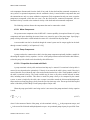
following equation:
2 ρ
K = 2∆PA ------2
m·
(2.3-3)
where
NUREG/CR-5535/Rev 1-Vol II
24
HYDRODYNAMICS
K
=
loss factor
∆P
=
nominal pressure drop (Pa)
A
=
junction area (m2)
ρ
=
fluid density (kg/m3)
m·
=
nominal mass flow rate (kg/s)
The value computed for K in this way may be very large because the default area is much larger than
the actual flow area. Also, critical flow would not be detected with this approach. Both the forward and
reverse loss coefficients should be equal unless there is a reason why they are physically different. In this
case, Equation (2.3-3) should be used to calculate the effective loss factor for both the forward and reverse
flow conditions (i.e., assume ∆P and m· also correspond to the reverse flow case). The geometric
relationship between the actual situation and the model is illustrated schematically in Figure 2.3-6.
In the case of minor flow paths that connect at branches having large main flows, a similar approach
can be used. In this case, let the junction area default to the minimum of the adjoining volumes
(presumably the area of the minor flow path) and use the smooth option (efvcahs with a = 0). The
determination of the loss factor may require some experimentation because of the possible large
momentum flux effect, which is ignored in the derivation of Equation (2.3-3). If one of the volumes is
quite large compared to the other, a modified Bernoulli equation can be used in which the overall loss
factor defined by Equation (2.3-3) can be replaced by K + 1. [In other words, the user-input loss factor is
computed by substituting K + 1 for K in Equation (2.3-3).]
All of the development herein assumes that known pressure drop flow relations exist for the singlephase case and that compressibility effects are small. If such is not the case, then the effective loss factor
values must be determined experimentally by running the code for a series of cases. Some experimentation
may be required, since the actual momentum flux calculation is complicated by several factors and may
differ slightly from the simple Bernoulli form.
Another problem relative to a minor leak path can occur when an incorrect flow rate through an
orifice for a given ∆P and loss coefficient K is calculated. As noted previously, this problem can be
avoided if the user inputs reasonable values for the flow area and the loss coefficient K, rather than
allowing the flow area to default and using a very large K.
2.3.4 Reflood Model
The reflood model is designed so that it can be activated at low pressure (less than 1.2 x 10⁶ Pa) with
nearly empty conditions (average void fraction in connected stack of hydraulic volumes > 0.9) or dryout
beginning (average void fraction > 0.1) or by user command through a trip. The model considers a heat-
25
NUREG/CR-5535/Rev 1-Vol II
HYDRODYNAMICS
Abrupt area change (jefvcahs = 00000100)
Aup
Ajunction
Adown
Athroat
Throat ratio =
Athroat
Ajunction
Physical situation with a loss factor Kactual
Smooth area change (jefvcahs = 00000000)
Aup
junction
A
----------------- A throat
Ajunction
Adown
2
Keffective = Kactual
Equivalent model with effective loss factor for the same pressure drop-flow relation
Figure 2.3-6 High-Resistance Flow Path Model
structure geometry composed of 1 to 99 heat structures as a reflood unit. As there is no input specification
for the length of a structure (except for the heat structure surface), such length is inferred from the length of
the boundary volume connected to the heat structure. It is the user’s responsibility to make certain that the
length of a heat structure corresponds to the length of its connected volume for reflood calculations.
Additional suggestions concerning the use of the reflood model are listed below:
NUREG/CR-5535/Rev 1-Vol II
26
HYDRODYNAMICS
1.
The appropriate user-specified maximum number of axial fine mesh intervals is 8 to
32. No significant differences have been found in using 16 to 128 axial nodes for 0.18m (0.6 ft) long heat structures.
2.
The appropriate length of hydrodynamic volumes is 0.15 to 0.61 m (0.5 to 2.0 ft).
3.
The maximum user-specified time step size is 0.01 to 0.05 seconds.
4.
Each reflood unit should have its own flow channel and parallel flow channels should
be connected by crossflow junctions.
The number of heat-structure geometries that can be specified for a reflood calculation is limited
only by computer storage capacity. Once the reflood model is activated for a particular heat-structure
geometry, only the structures where the critical heat flux are located will have a value in the critical heat
flux column of the output. The heat transfer modes that appear in the mode column of the major edit are the
same as those that appear when reflood is not activated except that 40 is added (see Section 3.2).
2.3.5 Noncondensables
The noncondensable model has the ability to be applied at every hydrodynamic volume in a system
model. While in operation, the model affects interface mass and heat transfer, wall heat transfer, and the
output of several variables that may cause discontinuities in plotted output. The purpose of this discussion
is to clarify the operation of the noncondensable model and its affect on the calculated results and to give
guidance for its use in system calculations.
In order to properly understand the operation of the noncondensable model, the fundamental
assumptions used in the model need to be discussed. First, the steam/noncondensable mixture is assumed
to be in thermal equilibrium. Second, the total pressure is the sum of the partial pressures of the steam and
the noncondensable. Next, the specific vapor internal energy is the mass weighted sum of the steam
specific internal energy and the noncondensable specific internal energy. Last, the saturation properties of
the liquid and steam are assumed to be a function of the partial pressure of the steam.
One of the effects of these assumptions is to force the phasic temperatures and the saturation
temperature to the same value. This causes a reduced driving potential for the interface mass and heat
transfer models. The interface heat transfer coefficients are reduced in the presence of noncondensables.
Consequently, low interfacial heat transfer regimes, such as the vertical stratification flow regime, may
give heat transfer coefficients that are too low for stable calculations (as evidenced by oscillatory
behavior). When this occurs, the vertical stratification model should be turned off on a volume basis. The
highest probability for this occurrence is under very low flow conditions.
A second problem may occur when noncondensables first appear in a system volume. At times, again
depending on the convection of noncondensable into the volume, the noncondensable iteration may fail or
water property errors occur at the minimum time step. This problem can usually be overcome by reducing
the size of the minimum time step. If this procedure fails, the convection rate or the concentration of the
27
NUREG/CR-5535/Rev 1-Vol II
HYDRODYNAMICS
noncondensable convection must be changed. This may be accomplished by modifying the boundary
conditions or by renodalizing the problem areas with acceptable thermodynamic conditions.
Last, the output from the code may contain discontinuities as noncondensables appear or disappear.
The variables that will have these discontinuities are the partial pressure of steam, phasic temperatures,
saturation temperature, vapor specific internal energy, and noncondensable quality. The partial pressure of
steam is set to the system pressure if noncondensables are not present, to 1.0 Pa if the volume state is pure
noncondensable, or to the calculated value otherwise. When a pure noncondensable is present in a volume,
all temperatures are set to equal values and are a function of the gas energy. As a fluid is injected into the
volume, the temperatures, the partial pressure of steam, and possibly the vapor energy will abruptly change
to new values based on the calculated thermodynamic conditions. Additionally, the liquid and saturation
temperature may appear at the fluid triple point value if the partial pressure of the steam is calculated to be
lower than the minimum fluid property table value.
As an example, a checkout problem used for development2.3-3 consisted of 322 K liquid water being
injected into 436 K helium. The liquid temperature and saturation temperature both changed from 436 to
273 K in one time step as the volume changed from a pure noncondensable state to a steam/
noncondensable mixture state. As more water was injected, the liquid transitioned to the correct value.
Selecting noncondensable input consists of specifying type and concentration of species on Cards
110 and 115 and by selecting options 4, 5, and 6 on the volume initial condition cards. Option 4, which
consists of pressure, temperature, and static quality at equilibrium conditions, is the easiest to use. A
restriction on the temperature is that it has to be less than the saturation temperature as a function of
pressure. Little experience has been obtained in using option 5 (equilibrium), and it has not been checked
out. Option 6 (nonequilibrium or equilibrium) is generally used to renode system models from Pygmalion
decks.2.3-4 See Volume I of this manual for the equations and variables used. If option 6 is selected, but
noncondensable quality is 0.0, the coding uses option 0. The static quality used in option 4 (equilibrium) is
Mg
- , where Mg = Ms + Mn.
given by ------------------Mg + Mf
The capability for initializing and performing transients with pure noncondensables has been
implemented. Input options 4 and 6 have provisions for initializing a system volume to a pure
noncondensable state. This is accomplished in option 4 by using the equilibrium quality variable as a flag.
By setting this quantity to 0, the logic specifies an ideal noncondensable gas equation of state. The variable
is reset to 1.0 for transient calculations. To use option 6 for initializing a pure noncondensable, both void
fraction and noncondensable quality must be set to 1.0 and the vapor energy must be set to a value that
gives the desired gas temperature.
The code will not allow a noncondensable to exist as just liquid water and no steam. The code will
Mg
–8
- ≥ 10 ). Thus, we recommend that users
add a little bit of steam (keeps steam quality X g = -------------------M g + Mn
input some steam when noncondensables and liquid water are present.
NUREG/CR-5535/Rev 1-Vol II
28
HYDRODYNAMICS
At the present time, option 4 is recommended. Only a saturated noncondensable state (100%
humidity) is obtained by this option. Improvement of input conveniences for initial noncondensable states
is under consideration. Users have reported some success with option 6 (nonequilibrium or equilibrium).
The users employ the following method. For a given total pressure (P), gas temperature (Tg), liquid
Mn
- , first calculate the
temperature (Tf), void fraction (αg), and noncondensable gas quality X n = -------------------
M n + M g
steam quality (Xs = 1 - Xn). The partial pressure of steam (Ps) is determined from the relation
P s = X s • P , which is true only if both steam and noncondensable are ideal gases, obey Dalton’s mixture
law, and have similar molecular weight. Using steam tables to get the steam energy (Us) from the known
values of Ps and Tg; then, calculate the noncondensable energy (Un) from Equations in Volume I of the
code manual. The mixture gas energy (Ug) is then calculated from equations in Volume I of the code
manual. Finally, the liquid energy (Uf) is determined using steam tables from the known values of P and
Tf.
Option 4, with static quality = 1.0, is recommended for containment volumes.
2.3.6 Water Packing
The volume control flag p is used to activate the water packing mitigation scheme. The scheme is
invoked if the detection criteria are met.
The number of partial time step repeats is shown in the hydrodynamic volume statistics block (time
step control information) in the major edit. Both the number of repeats since the last major edit and for the
whole calculation are shown.
2.3.7 Countercurrent Flow Limitation Model
The countercurrent flow limitation (CCFL) model (discussed in detail in Section 3 of Volume I) is
controlled by the junction control flag. The CCFL flag (f) can be used with a single-junction, pipe, annulus,
branch, valve, pump, and multiple junction. It cannot be used with a time-dependent junction, separator, jet
mixer, ECC mixer, turbine, or accumulator. Setting f = 1 will activate the CCFL model if all other
conditions are met, and setting f = 0 will not activate the model. The other conditions are as follows:
1.
The orientation of both the connecting volumes cannot be horizontal (i.e., the
elevation angle must be greater than or equal to 45 degrees).
2.
Both gas and liquid phases must be present.
3.
Countercurrent flow must exist, with liquid flowing down and gas flowing up.
As with the choking model, we recommend that if a junction is designated CCFL (f = 1), then an
adjacent junction should not be designated CCFL (f = 0). It is anticipated that this flag will find use in
29
NUREG/CR-5535/Rev 1-Vol II
HYDRODYNAMICS
activating the CCFL model in such internal structures as the upper core tie plate, downcomer annulus,
steam generator tube support plates, and entrance to the tube sheet in the steam generator inlet plenum.
Junction data cards can be used to input four quantities (junction hydraulic diameter, correlation
form, gas intercept, and slope). For these CCFL junction data cards, all four quantities must be entered
(must have five quantities for pipe and multiple junction). If no card is entered but the CCFL flag f is set to
1, then default values of the four quantities will be used. Presently, the default values are
Dj
=
A 1⁄2
2 -----j
π
β
=
0
c
=
1
m
=
1
This corresponds to a Wallis CCFL correlation with a gas intercept of 1 and a slope of 1, which,
according to Wallis,2.3-5 is the case for turbulent flow (m = 1) and when end effects are minimized (c = 1).
The input was made general so that the user can input CCFL correlations for the particular geometry
of interest. Wallis,2.3-5 Bankoff et al.,2.3-6 and Tien et al.2.3-7 discuss numerous examples, and these, along
with other references, should be consulted in order to justify the use of a particular correlation for a given
geometry. Wallis suggests m = 1 for a turbulent flow, c = 0.725 for tubes with sharp-edged flanges, and
c = 0.88 to 1.0 for tubes when end effects are minimized. Bankoff suggests β = tanh (γkcDj), where the
2π
critical wave number k c = ------ corresponds to the maximum wavelength that can be sustained on a
tp
interface of length tp (the plate thickness), and γ is the perforation ratio (fraction of plate area occupied by
holes). Bankoff suggests m = 1 and c of the form
c = 1.07 + 4.33 x 10⁻³D*
c=2
D* < 200
(2.3-4)
D* > 200
where D* is a Bond number defined as
ρ f – ρ g 1 ⁄ 2
D* = nπD g --------------
σ
NUREG/CR-5535/Rev 1-Vol II
(2.3-5)
30
HYDRODYNAMICS
and n is the number of holes. Tien uses the Kutateladze form (β = 1), but the form of c allows the Wallis
form also to be invoked for small diameters. He suggests c of the form
c = c7 [tanh c8 (D*)1/4]
where D* is a Bond number defined differently from Equation (2.3-5) as
g ( ρf – ρ g )
D = D ----------------------σ
*
1
--2
(2.3-6)
The values of m, c7, and c8 Tien found for four different conditions are provided in Table 2.3-1. With
regard to guidelines for plant-specific geometry (i.e., tie plates, support plates, etc.), flooding data obtained
in measurements from the plant geometry should be used to generate an appropriate CCFL model that can
be input with CCFL junction data cards.
Table 2.3-1 Values of m, c7, and c8 for Tien’s CCFL Correlation Form
m
c7
c8
Nozzle air supply with tapered inlet
0.8
2.1
0.9
Nozzle air supply with sharp edge inlet
0.8
2.1
0.8
Indirect air supply with tapered inlet and sharp
edge output
0.65
1.79
0.9
Indirect air supply with sharp edge inlet and
tapered output
0.65
1.79
0.8
Tests
Wallis,2.3-5 Bankoff,2.3-6 and Tien2.3-7 discuss the effects of viscosity, surface tension, and
subcooling on the correlations. At the present time, these effects have not been directly incorporated into
the form of the CCFL correlation used in RELAP5. We anticipate that these, particularly the subcooling
effects, will be addressed in future modifications to the code.
2.3.8 Level Tracking Model
The volume control flag 1 in t1pvbfe is used to activate the level tracking model as described in
Volume I. If more than one junction is connected to the top of the volume or if more than one junction is
connected to the bottom of the volume, the mixture level model is not used and is turned off.
If the volume control flag is set, the major edit will print out parameters associated with the mixture
level in the hydrodynamic volume. The parameters are voidla, the void above the level; voidlb, the void
below the level; vollev, the location of the level within the volume; and vlev, the velocity of the level
31
NUREG/CR-5535/Rev 1-Vol II
HYDRODYNAMICS
movement. The parameters voidla, voidlb, and vollev, can also be written to the restart-plot file if a
2080XXXX card is used and can be used in minor edit requests.
2.3.9 Thermal Stratification Model
The volume control flag t in t1pvbfe is used to turn on the subcell resolution scheme in the model.
The model is invoked if the detection criteria are satisfied. The model is intended for one-dimensional
components only.
The thermal stratification model should be used to improve the accuracy of calculations where there
is a warm fluid layer appearing above a cold fluid in a vertical stack of cells. A complete description of the
model is presented in Section 3 of Volume I.
2.3.10 Energy Conservation at an Abrupt Change
The junction control flag e in jefvcahs is used to activate the modification to the energy flux term
described in Volume I. This model is recommended for break junctions that connect to containment
volumes that are modeled using regular volumes (not time-dependent volumes).
2.3.11 Jet Junction Model
A single-junction (sngljun) component may be flagged as a jet junction. A j value of 1 on the junction
flags (jefvcahs) labels the junction as a jet junction. Jet junctions are used where subcooled water is
injected into the bottom of a stratified pool. The flag activates logic to increase the condensation rate on the
surface of the pool. Condensation is only enhanced in the volume above the jet when the volume is in
vertical stratification or a level exists from the level model. Normally the letters VST appear in the major
edits and 13 appears for the flow regime number (floreg) in the minor edits and on the restart-plot file
when vertical stratification exists in a volume and the letters LEV appear on the major edits and 14 appears
for the flow regime number (floreg) in the minor edits and on the restart-plot file when a level exists in a
volume from the level model. However, when the liquid interfacial coefficient has been altered by the jet
junction model and the volume is either in vertical stratification or a level exists from the level model, the
letters JET appear in the major edits and 15 appears for the flow regime number (floreg) in the minor edits
and on the restart-plot files.
2.3.12 References
2.3-1.
V. H. Ransom, et al. RELAP5/MOD2 Code Manual, Volume 3: Development Assessment
Problems. EGG-TFM-7952. Idaho National Engineering Laboratory. December 1987. pp. 14-17.
2.3-2.
Ibid. pp. 61-63.
2.3-3.
K. E. Carlson. Improvements to the RELAP5/MOD3 Noncondensable Model. EGG-EAST-8879.
Idaho National Engineering Laboratory. January 1990.
NUREG/CR-5535/Rev 1-Vol II
32
HYDRODYNAMICS
2.3-4.
W. H. Grush. Pygmalion. Idaho National Engineering Laboratory software. 1994.
2.3-5.
G. B. Wallis. One-Dimensional Two-Phase Flow. New York: McGraw-Hill. 1969. pp. 336-341.
2.3-6.
S. G. Bankoff, R. R. Tankin, M. C. Yuen, and C. L. Hsieh. “Countercurrent Flow of Air/Water
and Steam/Water Through a Horizontal Perforated Plate.” International Journal of Heat and
Mass Transfer. 24. 1981. pp. 1381-1385.
2.3-7.
C. L. Tien, K. S. Chuent, and C. P. Lin. Flooding in Two-Phase Countercurrent Flow. EPRI NP984. February 1979.
2.4 Hydrodynamic Components
The basic two-fluid model is applied uniformly to all volumes and junctions. Thus, the programming
design of the hydrodynamic calculation is primarily organized on volumes and junctions. Components are
organized collections of volumes and junctions and, to a lesser extent, the program is organized on
components. Components are designed for either input convenience or to specify additional specialized
processing. A pipe component is an example of a component designed for input convenience, since by
taking advantage of typical features of a pipe, several volumes and junctions can be described with little
more data than for one volume. Pump and valve components are examples of components requiring
additional processing. A pump component includes data defining pump head and torque characteristics for
single-phase and two-phase conditions as a function of pump angular velocity. A pump component
requires additional processing to advance the differential equation defining pump angular velocity. A valve
component requires additional data defining its characteristics and additional processing to calculate the
junction flow area as a function of valve position.
Components are numbered with a three-digit number, 001 - 999. Components need not be in strictly
consecutive order so that changes to a model of a hydrodynamic system requiring addition or deletion of
components are easily made. Volumes and junctions within a component are numbered by appending a six
digit number to the component number, CCCXXYYZZ. The CCC is the component number. At present,
YYZZ are zeros and XX is numbered consecutively starting at 01 for the volumes and junctions in the onedimensional components presently defined.
2.4.1 Common Features of Components
Each volume’s flow area, length, and volume must be supplied as input. As noted above, each onedimensional volume has a x-coordinate direction along which fluid flows in a positive or negative
direction, and may have y- and z-coordinate directions if crossflow connections are made to the volume.
The x-volume flow area is the volume cross-sectional area perpendicular to the x-coordinate direction. The
x-volume length is the length along the x-coordinate direction and similarly for the y- and z-coordinate
directions. The hydrodynamic numerical techniques require that the volume be equal to the volume flow
area times the length for each coordinate direction. This requirement is easily satisfied for constant area
volumes, but poses difficulties for irregular shaped volumes. Since it is very important that such a systems
code as RELAP5 conserves mass and energy, with momentum being an important but lesser consideration,
33
NUREG/CR-5535/Rev 1-Vol II
HYDRODYNAMICS
we recommend that an accurate volume be used; that the volume flow area be the cross-sectional area
averaged over the actual length of the volume; and the volume length be the quotient of the volume and the
flow area. The component input routines permit the volume, flow area, and length of each volume to be
entered as three nonzero positive numbers or two nonzero positive numbers and a zero. If three nonzero
quantities are entered, the volume must equal the flow area times length within a relative error of
0.000001. If one quantity is zero, that quantity is computed from the other two. The user need not be
concerned with y- or z-coordinate data unless crossflow connections are made, and even then only if the
default data for those coordinates are not satisfactory.
The volume horizontal angle specifies the orientation of the volume in the horizontal plane. The code
numerics have no requirement for this quantity; they were entered so a graphics package could be
developed to show isometric views of the system as an aid in model checking. Such a graphics package is
not included in RELAP5/MOD3.3. The horizontal angle is checked to verify that its absolute value is less
than or equal to 360 degrees, but no further use is made of the quantity.
The volume vertical angle specifies the vertical orientation of the volume. This quantity would also
be used in the graphics package and, in addition, specifies the vertical orientation of the volume coordinate
direction. The vertical angle must be within the range 90 to -90 degrees. The angle 0 degrees means the xcoordinate direction is in the horizontal plane; a positive angle means that the coordinate direction is
directed upward; a negative angle means it is directed downward. Slanted vertical orientation, such as an
angle equal to 45 degrees, is permitted. Note that as the vertical angle changes from zero, the y-coordinate
is always in the horizontal plane, and that the x- and z-coordinates, and their associated faces move out of
their original horizontal and vertical planes, respectively.
The coordinate direction implies the position of the inlet and outlet ends of the volume. The terms
inlet and outlet are convenient mnemonics relative to the coordinate direction but do not necessarily have
any relation to the fluid flow. The direction of fluid flow is indicated by the sign of the velocity relative to
the coordinate direction. For input convenience or ease in output interpretation, the coordinate direction
should be an easily remembered direction, such as the normal flow direction as opposed to the flow in an
accident situation.
As noted in the discussion of Figure 2.1-5, and described further below, a junction connects a
specified end of one volume to the specified end of another volume. This, in turn, establishes relative
positioning of the volumes. Because of gravity heads, the relative position is important to any volume with
a nonzero vertical component of a volume coordinate direction. If the coordinate direction in a volume
with a vertical component is reversed but no other changes are made, the inlet and outlet ends of the
volumes are also reversed. The physical problem is changed since the relative vertical positions of the
volumes are changed. If appropriate changes are made to junctions connecting the reversed volume, such
that the physical problem remains unchanged, the only change in the problem results would be a reversal in
the sign of the vector quantities associated with the volume. Furthermore, given a stack of vertically
oriented volumes, the proper gravity head is computed whether the direction coordinates are all upward, all
downward, or any random distribution. This assumes that junction connections are such that a vertical
NUREG/CR-5535/Rev 1-Vol II
34
HYDRODYNAMICS
stack is specified. As shown in Figure 2.1-5, a change in junction specification can change the relative
position of two volumes from two, vertically stacked volumes to a U-tube configuration.
Input for a volume includes the elevation change in a volume. For a straight pipe, the elevation
change (∆z) is related to the volume length (∆x) and the vertical angle (φ) by
∆z = ∆x sin φ .
(2.4-1)
Note that the elevation change associated with the x-coordinate has the same sign as the vertical
angle. To allow for irregularly shaped and curved volumes, the input elevation change is used for gravity
head calculations. Input checks are limited to the following: the magnitude of the elevation change must be
equal to or less than the volume length; and for the x-direction, the elevation change must be zero if the
vertical angle is zero; and the elevation change must be nonzero and have the same sign as the vertical
angle if the vertical angle is nonzero. The volume input does not need the elevation height of a volume
relative to an arbitrary base. The elevation change data performs the same function in determining gravity
heads.
If the hydrodynamic system has one or more loops, the user must ensure that the sum of the elevation
changes of the volumes in each loop is zero. A loop is any hydrodynamic flow path starting at a volume,
passing through one or more other volumes, and returning to the starting volume. If the net elevation
change in a loop is not zero, an incorrect gravity head exists; this is comparable to having an undesired
pump in the loop. This error is checked by the program. If closure is not within the error criterion of 0.0001
m, an input error will result.
The horizontal flow regime map is used rather than the vertical flow regime map when φ is less than
or equal to 45 degrees. Horizontal flow calculations include a horizontal stratified flow capability and a
horizontal stratified entrainment model.
Wall friction effects are computed from pipe roughness and hydraulic diameter data entered for each
volume. If the input x-direction hydraulic diameter (Dh,x) is zero, it is computed from the x-direction
volume flow area (Av,x),
D h, x =
4A v, x
------------π
(2.4-2)
If the input y-direction hydraulic diameter (Dh,y) is zero, it is computed from the y-direction volume
flow area (Av,y) and the x-direction volume flow area (Av,x), using the formula
4A v, y
D h, y = ---------------------0.5
( πA v, x )
(2.4-3)
35
NUREG/CR-5535/Rev 1-Vol II
HYDRODYNAMICS
If the input z-direction hydraulic diameter (Dh,z) is zero, it is computed from the z-direction volume
flow area (Av,z) and the x-direction volume flow area (Av,x), using the formula
4Av, z
D h, z = ---------------------0.5
( πA v, x )
(2.4-4)
The thermal stratification (t), level model (l), water packer (p), vertical stratification (v), and
equilibrium (e) flags can be entered only for the x- coordinate direction. The friction (f) flag can be entered
for the x-, y-, and z-coordinate directions.
A check is made that the pipe roughness is less than half the hydraulic diameter.
Most volumes allow seven control flags (tlpvbfe): the t flag is the thermal stratification flag; the l flag
is the level model flag; the p flag is the water packer flag; the v flag is the vertical stratification flag; the b
flag is the bundle interphase friction flag, recommended for cores and steam generators; the f flag
determines whether wall friction from the volume is to be included or neglected; the e flag controls
whether a nonequilibrium (two phases permitted to have unequal temperature) or an equilibrium (two
phases forced to have equal temperatures) calculation is used. Generally we recommend that wall friction
be computed in the x-direction and usually not in the y-direction, and that the nonequilibrium equation of
state be used.
System volumes require initial thermodynamic state conditions, and time-dependent volumes require
state conditions as a function of time or a time-advanced quantity. Seven options, numbered 0 through 6,
are available to specify state conditions. Options 0 through 3 specify water-only conditions and do not
allow a noncondensable gas. Option 0 requires pressure, liquid specific internal energy, vapor specific
internal energy, and void fraction. Options 1 and 2 always specify saturation conditions. Option 1 requires
saturation temperature and equilibrium quality. Option 2 requires saturation pressure and equilibrium
quality. Two phases are present if the quality is neither 0 nor 1. Option 3 always specifies single-phase
conditions and requires pressure and temperature. Options 1 through 3 can only specify equilibrium
conditions even if the nonequilibrium equation of state is requested. The next three options can specify the
presence of a noncondensable gas. Option 4 requires pressure, temperature, and equilibrium quality.
Equilibrium conditions are assumed, and the vapor consists of air and water vapor at 100% humidity.
Option 5 requires temperature, equilibrium quality, and noncondensable quality. Option 6 requires
pressure, liquid specific internal energy, vapor specific internal energy, void fraction, and noncondensable
quality.
For options 0 through 6, the boron concentration is assumed to be zero. If 10 is added to the above
option numbers, a boron concentration is required. See Section 3 of Volume I for a complete description of
the boron transport model. Boron is assumed to be only present in and to be convected by liquid water. If a
volume with liquid and boron has the liquid water removed by convection, the boron is also removed. If
the liquid water is evaporated, the boron remains. This is analogous to boron precipitating out as water is
NUREG/CR-5535/Rev 1-Vol II
36
HYDRODYNAMICS
evaporated. Infinite solubility of boron in water is assumed and boron remains in solution regardless of its
concentration until all of the liquid water disappears. Boron instantly redissolves the instant the quality
becomes less than 1. Boron concentrations are computed using only a boron continuity equation for each
volume. Boron is assumed to have no momentum, no internal energy, and to have no effect on the equation
of state.
Junctions connect two volumes by specifying a connection code for each volume. The connection
code specifies both the volume and a specific face of the volume. Except for a pipe component, current
components have only one volume, and a component reference is essentially a volume reference. The
connection codes for each component type are described in the beginning of the input description for that
component, as well as in Section 2.1.
The junction coordinate direction is from one volume end to another volume end and the input
description use the words FROM and TO to identify the connections. If a junction is reversed, the sign of
the vector quantities associated with the junction are reversed. To maintain the same physical problem, no
further changes are needed in other components. The initial velocities in reversed system junctions or timedependent velocities in time-dependent junctions should also be reversed.
Two quantities, the junction area and the junction area ratio, are defined from the user-supplied
junction area. These are printed in the major edit as JUN.AREA and THROAT RATIO. Junctions can
connect two volumes with possibly different volume flow areas, and the junction can also have a different
flow area. Two options are provided for calculating area change effects as the fluid flows through the
upstream volume flow area, the junction flow area, and the downstream volume flow area.
The smooth area change option uses only the stream tube form of the momentum equation that
includes spatial acceleration and wall friction terms. This option should be used when there are no area
changes or when the area changes are smooth, such as in a venturi. There are no restrictions on the usersupplied junction area for smooth area changes, and the junction area may be smaller than, larger than, or
between the adjacent volume flow areas. The junction flow area is set to the user-supplied flow area and
the junction area ratio is set to 1.0.
The abrupt area change option (a = 1) provides for area apportioning at branches, restricted junction
area, extra interphase drag (see Volume IV), and additional losses resulting from abrupt expansions, abrupt
contractions, orifices, and vena-contracta effects. The abrupt area change option (a = 2) includes
everything in the a = 1 option except for the losses. The user-supplied junction area (for a = 1 or a = 2)
must be equal to or less than the minimum of the adjacent volume flow areas for an abrupt area change.
The junction area is then set to the minimum of the adjacent volume flow areas, and the junction area ratio
is set to the ratio of the user-supplied junction area to the minimum of the adjacent volume flow areas.
When the user-supplied flow area equals the minimum of the adjacent volume flow areas, the junction area
ratio is 1.0, and the junction is a contraction/expansion. Program logic checks flow direction, and an
expansion with flow in one direction is treated as a contraction when flow reverses, and vice versa. If the
user-supplied junction area is less than the minimum of the adjacent volume flow areas, an orifice is
37
NUREG/CR-5535/Rev 1-Vol II
HYDRODYNAMICS
indicated, and the junction area ratio is less than one. Specifying the abrupt area change options (a = 1 or
a = 2) when there is no area change gives the same result as specifying the smooth area change option, but
slightly more computer time is required.
Valve junctions using any area change options vary the junction area ratio as the valve opens and
closes.
Junction velocities correspond to the junction flow area. Thus, the flow rate of a phase is the product
of the appropriate junction void fraction, the junction density (donored quantities), the junction velocity,
and the junction flow area. For orifices and valves, the actual flow velocity is higher at the minimum area,
which is the junction area multiplied by the junction area ratio. The junction area ratio is used to compute
the velocity at the minimum area when needed, such as in the choked flow model.
v junction A junction
v orifice = -----------------------------------A orifice
(2.4-5)
For user convenience, if the user-supplied junction area is zero, it is set to the minimum of the
adjacent volume flow areas regardless of the area change option. This is the proper default value for most
junctions, and only smooth area changes (where there is an area change) and orifices need nonzero usersupplied junction areas.
Junction user-inputted loss coefficients can be entered when additional losses above or instead of the
wall friction and abrupt area change losses are needed. These losses could arise from pipe bends,
irregularly shaped volumes, entrance or exit losses, or internal obstructions. Since the abrupt area change
loss model (a = 1) is only for sudden (i.e., sharp, blunt) area changes, it is in general too high and not
applicable for rounded or beveled area changes. The user input loss coefficients without using a = 1,
should be used for rounded or beveled area changes. Six coefficients are entered. Three are for forward
(positive) flow, where one is for the Reynolds number independent part and two are for the Reynolds
number dependent part. The other three are for reverse (negative) flow, where one is for the Reynolds
number independent part and two are for the Reynolds number dependent part. The coefficients are applied
to the junction dynamic pressure. Zero coefficients mean no additional losses are computed.
NUREG/CR-5535/Rev 1-Vol II
38
HYDRODYNAMICS
Table 2.4-1 shows the junction flow area, abrupt area change model loss, and user-input loss for area
change options a = 0, 1, and 2. The user input loss is optional in all three cases. For area change option
a = 1, the abrupt area change model loss and the optional user-input loss are additive.
Table 2.4-1 Area Change Options
Area change
option (a)
Junction flow
area
Abrupt area
change model
loss
User-input
loss
0
User-supplied
flow area
No
Optional
1
Minimum of
adjacent volume
flow areas
Yes
Optional
2
Minimum of
adjacent volume
flow areas
No
Optional
If junction user-supplied loss coefficients are entered and the abrupt area change option (a = 1 or
a = 2) is selected, the user should note that the junction area is set to the minimum of the adjacent volume
flow areas rather than the user-supplied flow area. Thus, the user-supplied loss coefficient needs to be
adjusted for the difference between the minimum of the adjacent volume flow areas and the user-supplied
junction flow area. For example, if the loss coefficient associated with the user-supplied flow area is Kj,
′
then the adjusted coefficient K j would be computed as:
2
A
′
K j = K j ------v2
Aj
(2.4-6)
where Aj is the user-supplied junction flow area and Av is the minimum of the adjacent volume flow areas.
It is important to note that RELAP5/MOD3.3 computes interfacial drag at junctions rather than
within volumes. This has important implications with respect to modeling reactor core bundles and steam
generator bundles. In these instances, the user should invoke the bundle interfacial drag model by
specifying b = 1 on the pipe volume control flags data card. In addition, in modeling grid spacers as
junctions within the core or steam generator bundle, the user should specify the junction area and hydraulic
diameter as equal to that for the bundle, rather than those characteristics of the grid spacer. The reason for
this is that the bundle interfacial drag model was formulated on the basis of bundle geometry. In order to
achieve the correct pressure drop at each grid spacer junction, the user should input a loss coefficient that is
adjusted for the difference between specifying bundle geometry rather than grid geometry. For example, if
39
NUREG/CR-5535/Rev 1-Vol II
HYDRODYNAMICS
′
the loss coefficient associated with the grid spacer is Kj, then the adjusted loss coefficient K j would be
computed as
′
Kj
2
A
= K j ------b2
Ag
(2.4-7)
where Ag is the flow area of the grid spacer and Ab is the flow area of the bundle. In modeling the upper
core tie plate, the user should specify the junction area and hydraulic diameter characteristics of the tie
plate. The reason is the CCFL model was formulated based on actual geometry.
Eight control flags are associated with junctions (jefvcahs). The j flag is the jet junction flag,
recommended at junctions where subcooled water is injected into the bottom of a pool. The e flag is the
energy correction flag, recommended at break junctions into a containment. The f flag is the CCFL model
flag, recommended for tie plates, downcomer annulus, etc. The v flag is the horizontal stratification
entrainment/pullthrough model flag, recommended at break junctions connected to horizontal volumes.
The c flag controls applications of the choking model.
The recommended input junction flags when the choking model is on (c = 0) are abrupt (a = 1 or 2)
and nonhomogeneous (h = 0). (1) With regard to the abrupt area options (a = 1 or 2), these are discussed in
Section 2.4.1. The full abrupt area change model (a = 1, code calculated losses) is recommended for
sudden (i.e., sharp, blunt) area changes, while the partial abrupt area change model (a = 2, no code
calculated losses, user input losses are to be used) is recommended for rounded or beveled area changes.
The extra interphase drag term (see Volume IV) in the abrupt area model (a = 1 or 2), helps ensure more
homogeneous flow that would be expected through a sudden area change. The smooth area change option
(a = 0) is recommended only for when there is no area changes or there are smooth area changes (i.e.,
venturi). (2) With regard to the nonhomogeneous (h = 0) option, it is generally recommended that h = 0 be
used. There may be rare situations where the combined interphase drag is too low, resulting in too much
slip and too low mass flow. For this situation, the homogeneous option (h = 1 or 2) is recommended.
(3) The user should monitor the calculated results for nonphysical choking. If this occurs, the user should
turn choking off (c = 1) at junctions where this occurs.
The a flag is for the area change option, and has already been discussed. The h flag controls the type
of momentum treatment; two-velocity, or one-velocity models. The two-velocity model is recommended
except as indicated above. The s flag controls whether the momentum flux is to be used.
System junctions require initial velocities, and time-dependent junctions require velocities as a
function of time. Two options are available to specify the velocities. One option requires the velocities; the
other requires mass flow rates from which the velocities are computed. If the flow is single-phase, the
velocity of the missing phase is set to that of the flowing phase. This matches the transient calculation that
computes equal phasic velocities when one phase is missing. The velocity conditions also require an
NUREG/CR-5535/Rev 1-Vol II
40
HYDRODYNAMICS
interface velocity. This input is for future capability involving moving volume interfaces. For now, the
interface velocity must be set to zero.
2.4.2 Time-Dependent Volume
A time-dependent volume must be used wherever fluid can enter or leave the system being
simulated. The geometry data required are similar to system volumes, but during input processing the
volume’s length, elevation change, and volume are set to zero. With the staggered mesh, the pressure
boundary would be applied in the center of the time-dependent volume. Setting these quantities to zero
moves the boundary to the edge of the system volume.
The state conditions as a function of time or some time-advanced quantity are entered as a table, with
time or the time-advanced quantity as the independent or search variable. The table must be ordered in
increasing values of the search variable, and each succeeding value of the search variable must be equal to
or greater than the preceding value. Linear interpolation is used if the search argument lies between search
variable entries. End point values are used if the search argument lies outside the search variable entries. If
constant state values are desired, only one set of data consisting of any search value and the associated
constant data needs to be entered. The program recognizes when only one set of data is entered, and
computer time is saved since the equation of state is evaluated only once rather than every time
advancement. Step changes can be accommodated by entering two adjacent sets of data with the same time
or an extremely small time difference.
The default search argument is time. If no trip number is entered, or if the trip number is zero, the
current advancement time is used as the search argument. When a nonzero trip number is entered, a unit
step function based on the time the trip was last set is applied. If the trip is false, the search argument is
-1.0. When the trip is true, the search argument is the current advancement time minus the last time the trip
was set. Thus, the search argument is always -1.0 when the trip is false and can range between zero and the
problem time when the trip is true. A time-dependent volume could have some constant condition when
the trip is false. In order to ensure proper operation for the constant condition, both a card with a negative
search argument and a card with a zero search argument need to be entered (see example in Volume V).
When the trip is true, it could follow a prescribed function of time where the time origin is the time of the
trip not the start of the transient.
Through an input option, nearly any time-advanced quantity can be specified as the search argument.
The allowed quantities are listed in the input description. The search variables in the table are assumed to
have the same units as the search argument, and the table lookup, interpolation, and treatment of out of
range arguments are identical to those described for the default time argument. However, handling of trips
is different. If the trip number is zero, the current value of the specified time-advanced variable is used. If
the trip number is nonzero, the time delay cannot be applied as for the default time case, since the search
argument may not be time. Thus, if the trip is false, the search argument is -1.0E75; if the trip is true, the
current value of the specified variable is the search argument.
41
NUREG/CR-5535/Rev 1-Vol II
HYDRODYNAMICS
When time is the search argument, the current value is the value at the end of the time step; for any
other variable, the current value is the value at the beginning of the time step. Time is the default search
argument, but time can also be specified as the search argument through the input option of naming a timeadvanced variable. These two uses of time as the search argument are different if a trip is used, since the
default method can apply a time delay and the other cannot.
2.4.3 Time-Dependent Junction
Time-dependent junctions can be used whenever the phasic velocities or phasic mass flow rates are
known as a function of time or other time-advanced quantity. Time-dependent junctions can connect any
two system volumes, or a system volume and a time-dependent volume. Phasic mass flow rates are
converted to phasic velocities using the upstream phasic densities. Examples of their use would be to
model a constant displacement pump in a fill system, a pump or a valve (or both), by using an associated
control system or measured experimental data. Time-dependent junctions are also used frequently in test
problems to check code operation.
The phasic velocities or mass flows in the time-dependent junction as a function of time or the timeadvanced quantity are entered as a table, with time or the time-advanced quantity as the independent or
search variable. The requirements, interpolation, and trip logic are identical to that for time-dependent
volumes.
The capability of using time-advanced quantities as search arguments can be used to model pressuredependent water injection systems. If the injection flow is a function of the pressure at the injection point,
the volume pressure at that point is used as the search argument. A trip is defined to be true when the
injection system is actuated. Entry of table data with a negative pressure and zero flows causes the flow to
be zero when the trip is false. In order to ensure proper operation for zero flow, both a card with negative
pressure and a card with a zero pressure need to be entered (see example in Volume V). The remaining
table entries define the injection flow as a function of positive pressures. The source of injection water is a
time-dependent volume. The pressure of the water supplied by the time-dependent volume could also be a
function of the pressure at the injection volume to represent the work of pumping the water into the system.
If the injection flow is a function of a pressure difference, the pressure difference can be defined by a
control system variable, and that control variable is then defined as the search argument.
Some uses of time-dependent junctions can cause modeling difficulties. When using a timedependent junction to specify flow from a time-dependent volume into the system, the incoming phasic
densities, void fractions, phasic velocities, phasic mass flow, and phasic energies can be specified. But
when using a time-dependent junction to specify flow out of a system, the densities, void fractions, and
energies of the fluid leaving the system are not known in advance. Thus, use of time-dependent junctions
to control outflow is not recommended. The following is one example of a modeling problem. The user
anticipates that a volume will contain only vapor and accordingly sets a time-dependent junction to a
nonzero vapor flow and zero liquid flow. If the user anticipated incorrectly and liquid condenses or is
carried into the volume, the liquid will accumulate unrealistically since it cannot leave the system.
NUREG/CR-5535/Rev 1-Vol II
42
HYDRODYNAMICS
In a simple pipe modeling application, a time-dependent volume and junction can be used to specify
the inlet flow. Likewise, a time-dependent volume and junction can model the feedwater flow into a
reactor steam generator. Controlling the fluid flow out of the pipe or controlling the water/steam flow out
of the steam generator through a time-dependent junction is not recommended. If a system junction (flows
computed by the simulation rather than specified as boundary conditions) connected to a time-dependent
volume is not sufficient, perhaps a servo valve can provide the required simulation.
2.4.4 Single-Volume
A single-volume component is simply one system volume. A single-volume can also be described as
a pipe component containing only one volume. This single-volume component uses fewer input cards and
fewer data items than does a pipe component. However, if the single-volume might be divided into several
volumes for nodalization studies, we suggest the pipe component, since such changes are quite easy for
pipes.
2.4.5 Single-Junction
A single-junction component is simply one system junction. It is used to connect other components
such as two pipes. Initial junction conditions can be phasic velocities or phasic mass flow rates.
2.4.6 Pipe
A pipe component is a series of volumes and interior junctions, the number of junctions being one
less than the number of volumes, and the junctions connect the outlet of one volume to the inlet of the next
volume. Pipe components can be used for those portions of the system without branches. Pipe components
offer input conveniences, since most characteristics of the volumes and junctions in a pipe are similar or
change infrequently along the pipe, and input data requirements can be reduced accordingly. Because of
the sequential connection of the volumes, junctions are generated automatically rather than being
individually described. Although the input is designed to assume considerable similarity in volume and
junction characteristics, any of the volume and junction features (such as flow area, orientation, pipe
roughness, or control flags) can be changed at each volume or junction.
2.4.7 Branch
Branch components are provided to model interconnected piping networks. The branching model is
based on one-dimensional fluid flow, which is adequate for most cases of branching and merging flow.
Such situations include wyes, parallel flow paths from upper and lower plenums, and any branch from a
vessel of large cross-section. For branching situations where phase separation effects caused by
momentum or gravity are important, an approximate mapping technique can be used to map the twodimensional situation into the one-dimensional space of the fluid model.
A branch component consists of one system volume and zero to nine junctions. The limit of nine
junctions is due to a card numbering constraint. Junctions from other components, such as single-junction,
43
NUREG/CR-5535/Rev 1-Vol II
HYDRODYNAMICS
pump, other branch, or even time-dependent junction components, may be connected to the branch
component. The results are identical whether junctions are attached to the branch volume as part of the
branch component or are in other components. Use of junctions connected to the branch, but defined in
other components, is required in the case of pump and valve components and may also be used to attach
more than the maximum of nine junctions that can be described in the branch component input.
2.4.8 Pump
The pump component model can be separated into models for hydrodynamics, pump-fluid
interaction, and pump driving torque. The pump component input provides information for the
hydrodynamic and pump-fluid interaction models and may optionally include input for an electric motor to
drive the pump. A pump may also be connected to a shaft that is a specialized component within the
control system. A shaft component is used when the pump is driven by a turbine or by an electric motor
with a control system to regulate speed.
2.4.8.1 Pump Model Description.
The hydrodynamic model of a pump component consists of one volume and two associated
junctions. The coordinate directions of the junctions are aligned with the coordinate direction of the
volume. One junction is connected to the inlet and is called the suction junction; the other junction is
connected to the outlet and is called the discharge junction. The pump head, torque, and angular velocity
are computed using volume densities and velocities. The head developed by the pump is divided equally
and treated like a body force in the momentum equations for each junction. With the exception of the head
term, the hydrodynamic model for the pump volume and junctions is identical to that for normal volumes
and junctions.
2.4.8.1.1 Pump Performance Modeling
Interaction of the pump and the fluid is described by empirically developed curves relating pump
head and torque to the volumetric flow and pump angular velocity. Pump characteristic curves, frequently
referred to as four-quadrant curves, present the information in terms of actual head (H), torque (τ),
volumetric flow (Q), and angular velocity (ω or N). These data are generally available from pump
manufacturers. For use in RELAP5, the four-quadrant curves must be converted to a more condensed
form, called homologous curves, which use dimensionless quantities. The dimensionless quantities involve
the head ratio, torque ratio, volumetric flow ratio, and angular velocity ratio, where the ratios are actual
values divided by rated values. The rated values are also required pump component input and correspond
to the design point or point of maximum efficiency for the pump.
The homologous curves are entered in tabular form, and the dependent variable is obtained as a
function of the independent variable by a table search and linear interpolation scheme. There is a separate
set of curves for head and torque, and each set is composed of eight curves. Not all the regimes need be
described by the input, but a problem is terminated if an empty table is referenced. Both head and torque
data must be entered for the regimes that are described with input.
NUREG/CR-5535/Rev 1-Vol II
44
HYDRODYNAMICS
The homologous curves for pump head and torque are for single-phase operation. These same tables
are used by the two-phase pump model, but additional data must be input to model two-phase degradation
effects.
Pump head data are always used in the momentum equations. Torque data may or may not be used in
computing pump rotational velocity, depending on the pump motor model selected and if it is energized or
not. However, both head and torque are used to determine pump energy dissipation, and consistent data
must therefore be entered. The pump homologous data should be checked by computing pump efficiency
from the homologous data. No such checking is currently included in RELAP5, nor is the operating
efficiency edited on major edits.
The sign conventions for various pump quantities are as follows: a pump operating in the normal
pump regime has a positive angular velocity; the volumetric flow is positive if it is in the same direction as
the volume coordinate direction; the head is positive if it accelerates the flow in the volume coordinate
direction; and the torque is that exerted by the fluid on the pump and is negative if it tends to decelerate the
pump. In normal pump regimes and in steady-state, this torque is negative and is balanced by the positive
torque from the pump motor.
2.4.8.1.2 Pump Data Homologous Representation
The use of pump performance data in terms of nondimensional homologous parameters is often
confusing. The purpose of this discussion is to briefly outline rules for a procedure to properly use the
homologous data.
The homologous parameters for pumps are obtained from dimensional analysis that can only provide
the conditions for similarity. Three independent parameters are obtained from application of
Buckingham’s Pi theorem.2.4-1 They are
Q
π 1 = ------νD
(2.4-8)
1
--2
NQ
π 2 = --------------3
( gH )
(2.4-9)
--4
Q
π 3 = -----------3
ND
(2.4-10)
A fourth parameter that is commonly used can be obtained by a combination of π2 and π3 to yield
45
NUREG/CR-5535/Rev 1-Vol II
HYDRODYNAMICS
gH
π 4 = -----------2 2
N D
(2.4-11)
The first parameter, π1, is analogous to a Reynolds number and is the only parameter involving the
fluid kinematic viscosity, ν. Experience with pump design and scaling has shown that viscous effects
caused by skin friction are small, especially for high Reynolds number flows, and, in practice, the
requirement to maintain π1 constant is not used. The use of π2, π3, and π4 to correlate pump performance
has proven quite useful. The parameter π2 is called the specific speed and is often used as a single
parameter to characterize the type of pump impeller best suited for a particular application. In practice, the
acceleration of gravity, g, is omitted, and the specific speed is simply defined as
1
--2
NQ
N s = ---------3
H
(2.4-12)
--4
where the speed N is in rpm, the capacity Q is in gpm, and the head H is in ft. In this form, Ns is not
dimensionless but has a history of usage that still persists.
Two performance parameters that are used for pump modeling are the specific nondimensional
capacity,
Q
Q s = -----------3
ND
(2.4-13)
and the specific head (dimensional due to omission of the gravitational acceleration constant),
H
H s = -----------2 2
N D
(2.4-14)
The D that appears in Equations (2.4-13) and (2.4-14) is a characteristic dimension of the pump and
is assumed to be the impeller diameter. When scaling pump performance using homologous parameters,
the implication is that all pump dimensions are geometrically similar (i.e., changing D implies a
proportional change in impeller width, leakage paths, and in all linear dimensions of the pump).
When the pump torque performance is included, one additional dimensionless parameter is obtained
from dimensional analysis and is
NUREG/CR-5535/Rev 1-Vol II
46
HYDRODYNAMICS
τ
π 5 = ---------------2 5
ρN D
(2.4-15)
where π5 is the nondimensional specific torque.
Generally, constant density is assumed, so the dimensional specific torque used in constructing the
homologous representation is reduced to
τ
π s = -----------2 5
N D
(2.4-16)
Homologous states are states for which specific capacity, head, and torque are all constant. Thus, at
any state it is possible, within the limitations of similarity theory, to predict the performance for other
combinations of speed, head, and flow that have the same homologous state. It is also possible to scale
pump performance with reasonable accuracy to account for changes in physical pump size through the
diameter D by keeping the homologous parameters fixed.
Pump performance data are usually displayed by plotting head and torque as functions of speed and
volumetric flow. Figure 2.4-1 is a four-quadrant pump curve for the Semiscale MOD1 pump, and has
speed and flow as independent variables with lines of constant head.
Figure 2.4-2 is a comparable four-quadrant plot of the Semiscale MOD1 pump torque data. All
possible operating states of the pump are represented on such plots. These data for a particular pump can
be approximately collapsed into a single curve by nondimensionalizing specific head and capacity
parameters for corresponding homologous operating points using the design point values for head,
capacity, and speed.
All points on Figure 2.4-1 having the same specific capacity are straight lines passing through the
origin (lines of constant Q/N). The impeller diameter is omitted from the homologous parameters since it is
constant for a particular pump. The design operating point is indicated by the cross. The line of constant Q/
N, passing through the design point and its reflection about the ordinate divides each quadrant into two
47
NUREG/CR-5535/Rev 1-Vol II
HYDRODYNAMICS
=0
3000
Homologous states
Normal
+
H
Dissipation
HAN
SPEED (rpm)
4000
HAD
2000
HVN
-20 ft
HVD
1000
150 ft75 ft 40 ft
200 ft100 ft 20 ft
50 ft
10 ft
-10 ft
H=
-200 -100
-50 ft
100
Volumetric flow
(GPM)
300
0
HVT
-1000
Turbine
200
-100 ft
-150 ft
-2000
HAT
HVR
Reverse
HAR
Figure 2.4-1 Four-Quadrant Head Curve for Semiscale Mod1 Pump (ANC-A-2083)
NUREG/CR-5535/Rev 1-Vol II
48
Dissipation
BAD
Line of constant Q/N
(rpm)
Speed
HYDRODYNAMICS
Normal
BAN
3000
BVN
2000
200
150
100
BVD
1000
50
25
-300
BVT
-200
Volumetric
Flow (GPM)
τ=0
-100
100
200
300
BVR
-25
-50
-100
-150
-1000
τ=0
-200 in. -lb
Turbine
-2000
BAT
Reverse
BAR
Figure 2.4-2 Four-Quadrant Torque Curve for Semiscale Mod1 Pump (ANC-A-3449)
49
NUREG/CR-5535/Rev 1-Vol II
HYDRODYNAMICS
octants. Each of these eight octants is named according to the convention listed in Table 2.4-2, for the
purpose of constructing the homologous representation.
Table 2.4-2 Pump Homologous Curve Definitions
Regime
number
Regime
mode
ID name
α
1
HAN BAN
Normal
pump
>0
>0
<1
2
HVN BVN
Normal
pump
>0
>0
3
HAD BAD
Energy
dissipation
>0
4
HVD BVD
Energy
dissipation
5
Dependenta
variable
head
Dependenta
variable
torque
v/α
h/α2
β/α2
>1
α/v
h/v2
β/v2
<0
> -1
v/α
h/α2
β/α2
>0
<0
< -1
α/v
h/v2
β/v2
HAT BAT
Normal
turbine
<0
<0
<1
v/α
h/α2
β/α2
6
HVT BVT
Normal
turbine
<0
<0
>1
α/v
h/v2
β/v2
7
HAR BAR
Reverse
pump
<0
>0
> -1
v/α
h/α2
β/α2
8
HVR BVR
Reverse
pump
<0
>0
< -1
α/v
h/v2
β/v2
v
v/α
Independent
variablea
a. α = rotational ratio; v = volumetric flow ratio; h = head ratio; and β = torque ratio.
The four-quadrant pump head and torque maps in Figure 2.4-1 and Figure 2.4-2 can be reduced to
the homologous representation curves in two steps. First, the maps are made dimensionless by using the
rated head, HR, flow, QR, speed, NR, and torque, τR, to form corresponding dimensionless parameters
N
H
Q
τ
h = ------- , v = ------- , α = ------- , and β = ----- , respectively. Second, the data are plotted in terms of the
HR
QR
NR
τR
NUREG/CR-5535/Rev 1-Vol II
50
HYDRODYNAMICS
homologous parameter h/α2 or h/v2, v/α or α/v, and β/α2 or β/v2. The parameter used depends upon the
octant in which the curve is being plotted. The choice is made so that the values are bounded (i.e., the
denominators never vanish and, in the case of the capacity parameter, the range of variation is confined
between plus and minus 1.0). Figure 2.4-3 is the homologous head curve that is obtained from the head
map in Figure 2.4-1. Note that not all points fall on a single curve. This is a result of the inexact nature of
the similarity theory. Real pumps do not perform exactly according to the similarity relations due to
leakage, viscous effects, etc.; however, the correspondence is surprisingly close, as evidenced by the tight
clustering of points. The homologous curve for the torque data of Figure 2.4-2 is shown on Figure 2.4-4.
Since the data do not form a single curve, the design operating usual approach is to use least squares or
other smoothing techniques to obtain curves passing through the point (1.0, 1.0). These curves must also be
continuous at the point v/α or α/v equal to + 1.0. The legends on Figure 2.4-3 and Figure 2.4-4 have a key
indicating which of the homologous parameters are used in each octant. All combinations of head, flow,
speed, and torque can now be located on a corresponding segment of the homologous curve. Note that the
impeller diameter parameter that appears in the dimensionless similarity parameters is not used in the
homologous reduction of the four-quadrant representation; thus, special considerations are necessary for
application of the data to a larger but geometrically similar pump. The advantage of using the homologous
pump performance data representation in a computer code is obvious. Two-dimensional data arrays and
two-dimensional interpolation are avoided, and, only two parameter tables and one-dimensional
interpolation are required.
2.4.8.1.3 Homologous Data and Scaling
In most system simulation tasks, complete pump performance data are not available. Usually, only
first-quadrant data are available (normal operation), and sometimes only the design or rated values are
known. In the case of full-scale nuclear power plant pumps, it is difficult to test the pumps in all octants of
operation or even very far from design conditions. The usual approach to obtain data for such systems is
through the use of scaled-down pump tests.
The scaled pump test data can be for the same physical pump operated at reduced speed or for a
pump scaled in size such that similarity is preserved. For the case of a pump scaled in size, it is necessary
to maintain the similarity in specific head, capacity, speed, and torque parameters. (Note that the diameter
was dropped in the development of the homologous performance model since a fixed configuration was
considered.) Consideration of the diameter change must be implicitly included in the selection of “rated”
parameters to properly account for changes in geometric scale. The homologous parameters, including the
impeller diameter, are given in Equations (2.4-13), (2.4-14), and (2.4-16). When a change in scale is
considered, an additional degree of freedom is possible, since only two parameters, the rated specific head
and capacity, must be held constant. The specific speed is also held fixed whenever both specific head and
capacity are kept fixed. There are many combinations of N and D for which this is possible.
The usual situation encountered in applications work is that homologous data exist for a similar
pump, and the question arises, “Can we use these data to simulate our pump by adjusting the rated
parameters?” The question can best be answered by the following statements. First, the best approach is to
51
NUREG/CR-5535/Rev 1-Vol II
HYDRODYNAMICS
Normal (+ Q, +N)
HAN
HVN
Dissipation (-Q, +N)
HAD
HVD
Turbine (-Q, -N)
HAT
HVT
h/α2 or h/v2
HAD
1.5
HAT
HAN
Reverse (+Q, -N)
HVD
HAR
HVR
1.0
HVT
Denotes head (H)
HAR
0.5
HVN
Denotes division by
α or α2 (A)
}
v or v2 (V)
-0.5
0.5
v/α or
α/v
HVR
Denotes quadrant N, D, T, R
-0.5
Figure 2.4-3 Homologous Head Curve
use the rated conditions corresponding to the pump used to generate the data. Second, the rated condition
can be changed if the specific head and capacity are kept the same as for the pump used to generate the
data. Similarity is assured since the modeled pump will have the same specific speed. The rated conditions
by definition locate the region of pump operation on the homologous performance curve, at the design
point or point of maximum efficiency. The rated conditions can then be safely adjusted in this way. They
can also be adjusted using the impeller diameter as an additional parameter while still maintaining the rated
specific speed, head, and capacity constant. However, this type of scaling implies a change in pump
NUREG/CR-5535/Rev 1-Vol II
52
HYDRODYNAMICS
Normal (+ Q, +N)
BAN
BVN
Dissipation (-Q, +N)
BAD
BVD
1.0
β/α2 or β/v2
BAN
BAD
BVN
BVD
Turbine (-Q, -N)
BAT
BVT
Reverse (+Q, -N)
BAR
BVR -1.0
BVT
-0.5
0.5
0
BAT
1.0
v/α
or
α/v
-0.5
Denotes torque (B)
BVR
BAR
Denotes division by
α or α2 (A)
v or v2 (V)
-1.0
}
Denotes quadrant N, D, T, R
Figure 2.4-4 Homologous Torque Curve
geometry and the extrapolation depends more heavily on the validity of the pump similarity relationships,
which are only approximate. In all cases, the rated conditions must correspond to the same specific speed
as the pump used to produce the data. However, the operating point does not have to correspond to the
rated conditions. In such a case, the pump will operate at off-design conditions and efficiency will be less
than the design value. Such off-design adjustments may be desirable to better match the modeled pump
head-flow characteristics at the system operating point.
53
NUREG/CR-5535/Rev 1-Vol II
HYDRODYNAMICS
2.4.8.1.4 Two-Phase Performance Representation
The discussion above applies to a pump operated with a single-phase fluid of constant density. When
pump performance operation with a two-phase fluid is considered, the homologous representation of
performance data has a less firm basis. An empirical modification of the homologous approach has
therefore been developed based on Semiscale and Westinghouse Canada Limited (WCL) data. The
RELAP5 two-phase pump model is the same as that developed for RELAP4.2.4-2 The approach is one in
which the two-phase performance data are plotted, and a lowest performance envelope is constructed. This
curve is called the fully degraded two-phase performance. The fully degraded performance and the singlephase performance data are used to form two-phase difference homologous performance curves for head or
torque. The pump performance is then expressed in terms of the single-phase data and the difference data
using a two-phase multiplier that is a function of void fraction. The pump head is expressed as
H = H1φ - MH(αg) ∆H
(2.4-17)
where ∆H is the head difference obtained from the single-phase to two-phase difference homologous
curve. The function MH(αg) is the two-phase multiplier, defined such that it is zero for the void fraction,
αg, equal to 0.0 and 1.0. The pump torque is expressed in a similar way. Very little advice can be offered
with respect to scaling of the two-phase performance data. Generally, it is assumed that the same similarity
principles used for single-phase performance also hold for two-phase performance. A complete set of data
was generated for a Semiscale pump, and these data are widely used for predicting two-phase performance
of other pumps.
2.4.8.1.5 Pump Velocity Modeling
The pump computation for a time step begins by computing pump head and torque from the
homologous data using pump angular velocity and volume conditions at the beginning of the time step.
The head is used in the momentum equations. The remaining pump calculation determines the pump
angular velocity at the end of the time step. The logic for computing pump angular velocity is complex,
since stop logic, friction, an initializing calculation, the presence or absence of two tables, and two trips are
involved. Additional capability is provided if the pump is associated with a shaft component. An optional
card in the pump component input data specifies whether the pump is associated with a shaft. The
remainder of this section defines pump capability when not associated with a shaft. In Section 4.2.3, the
available shaft component capabilities are described and user suggestions are given.
Pump frictional torque (τfr) is modeled as a cubic function of the pump rotational velocity and is
given by
ω + τ ω 2 + τ ω 3
τ fr = ± τ fr0 + τ fr1 -----fr2 -----fr3 ------
ωR
ωR
ωR
NUREG/CR-5535/Rev 1-Vol II
(2.4-18)
54
HYDRODYNAMICS
where ω is the pump rotational velocity; ωR is the rated pump rotational velocity; and τfr0, τfr1, τfr2, and
ω
ω
τfr3 are input data. The pump friction torque is negative if ------ > 0 , and it is positive if ------ < 0 .
ωR
ωR
The pump model has special capabilities to accommodate experimental systems. For example; the
LOFT system primary pumps use a motor-generator, flywheel, fluid coupling, and an active control system
in order to better represent full-size PWR pumps. Allowing a variable pump inertia provides a simple
model of the LOFT pump rotational behavior. To facilitate LOFT usage, pump input provides for constant
inertia or optionally allows input of variable inertia data. The variable pump inertia (Ip) is given by
I p = I pn
ω <S
for -----L
ωR
ω +I ω 2+I ω
I p = I p0 + I p1 -----p2 -----p3 -----ωR
ωR
ωR
(2.4-19)
ω ≥S
for -----L
ωR
3
(2.4-20)
where ω is the pump rotational velocity, ωR is the rated pump rotational velocity, and Ipn, Ip0, Ip1, Ip2, Ip3,
and SL are input data.
A pump stop card containing limits on problem time, forward pump angular velocity, and reverse
angular velocity may optionally be entered. The pump angular velocity is set to zero and remains zero for
the remainder of the problem if any of the limits are exceeded. Selected tests can effectively be disabled by
entering a very large number for the limits. If the problem time limit = 0, then the problem time test is
ignored.
A time-dependent pump velocity table and an associated trip number may be entered. If the table is
entered and the trip number is zero, the pump angular velocity is always determined from this table. If the
trip number is nonzero, the table is used only when the trip is true. The default search variable for the timedependent pump velocity table is time, but time-advanced quantities may be specified as the search
variable. When time is the search variable by default, the search argument is time minus the time of the
trip. When a time-advanced variable is specified as the search variable (even if it is time), the search
argument is just the specified variable. The use of the pump velocity implies a pump motor to drive the
pump at the specified velocity.
The following is a possible example of the use of a time-advanced variable as the search argument in
the pump velocity table. The motor and its control system that drives a BWR recirculation pump could be
modeled using the control system with one of the control variables representing the rotational velocity of
the motor. The recirculation pump would be modeled as a hydrodynamic pump component. The torque
exerted by the water on the pump would be one of the input variables to the control system model. Motor
velocity would be supplied to the pump component by specifying the motor velocity as the search
argument of the time-dependent pump velocity table. The table would relate the motor rotational velocity
55
NUREG/CR-5535/Rev 1-Vol II
HYDRODYNAMICS
to the pump rotational velocity. If the motor and pump were directly coupled, the search variables and
dependent variables would be the same.
Whenever the time-dependent pump angular velocity table is not being used, the pump angular
velocity is determined by the advancement in time of the differential equation relating pump moment of
inertia, angular acceleration, and net torque. The net torque is the pump motor torque minus the
homologous torque value and the frictional torque. If the pump trip is false, electric power is being
supplied to the pump motor; if the trip is true, electric power is disconnected from the pump motor and the
pump motor torque is zero. If a table of pump motor torque as a function of pump angular velocity is
entered, the pump motor is directly specified and motor torque is obtained from the table, interpolating
when needed. If the table is missing, the pump motor is implied and torque is assumed to be such that the
net torque is zero. This is implemented in the program by simply setting the pump angular velocity at the
end of the time step equal to that at the beginning of the time step. This latter option is usually used when
the problem starts with the pump at its normal steady-state velocity; the pump is assumed to remain at this
velocity until the pump trip, and the trip, once true, remains true for the rest of the problem.
2.4.8.2 Pump Modeling Examples.
Two examples are discussed to illustrate pump operation. Consider a pump in a closed loop filled
with liquid water. At the start of the transient, all the water in the loop is at zero velocity but the pump is
rotating in the positive direction. No pump motor torque table is used, the pump trip is initially false, and
thus, the pump angular velocity is constant at the initial value until the pump trip becomes true. With the
pump rotating at a constant angular velocity but the water at rest, the head is high and the water is
accelerated. As the velocity of the water increases, wall friction and area change losses increase because of
the dependence of these losses on water velocity. At the same time, the pump head obtained from the
homologous data will decrease as the volumetric flow increases. A steady-state will be reached when the
pump head and the loss effects balance. If no wall friction options are selected for the loop piping and no
area losses are present, the water will accelerate until the pump head is zero. When steady-state is reached
and the pump trip is then set true, the pump will begin to decelerate because the pump friction torque and
the torque exerted by the water on the pump are no longer balanced by the pump motor torque. The water
also begins to decelerate owing to loss effects. The interaction between the water and pump depends on the
relative inertias and friction losses between the two. If the water tends to decelerate more rapidly than the
pump, the pump will use its rotational kinetic energy to maintain water velocity. If the pump tends to
decelerate more rapidly than the water, the pump, depending on its design as reflected in the homologous
data, may continue to act as a pump or the kinetic energy of the water may tend to maintain pump angular
velocity.
The second example is similar to the first example except that the initial pump angular rotational
velocity is zero and a pump motor torque curve for an induction motor is used. From the curve, the torque
is positive at zero angular velocity and increases slowly as the velocity increases to a value slightly below
the synchronous speed. Then, the torque decreases sharply to zero at the synchronous speed and continues
to negative torque. At the initial conditions, the net torque is positive, the pump angular velocity increases,
NUREG/CR-5535/Rev 1-Vol II
56
HYDRODYNAMICS
and the water is accelerated. If the pump torque is sufficiently high, the pump velocity increases to slightly
below the synchronous speed where the developed torque matches the frictional torque and the torque
imposed by the water. As the water accelerates, the angular velocity decreases slightly to meet the
increased torque requirements. The angular velocity decrease is very small owing to the steep slope of the
torque versus angular velocity near the synchronous speed. Thus, once the pump approaches the
synchronous speed, the transient behavior of the second example is similar to the first example.
2.4.8.3 Built-in Pump Data.
RELAP5 contains built-in, single-phase homologous data for a Bingham Pump Company pump with
a specific speed of 4,200 and a Westinghouse Electric Corporation pump with a specific speed of 5,200.
Two-phase difference homologous data are also associated with these pumps, but the data curves are
identical and were obtained from two-phase tests of the Semiscale pump. (The data curves are stored as
data statements in subroutine RPUMP.) No built-in, two-phase multiplier tables are entered. Specification
of built-in, single-phase homologous data does not require specification of the built-in, two-phase
difference homologous data, or vice versa.
If multiple pump components are used and some tables are common to more than one component,
then user effort and computer storage can be saved by entering the data for only one component and
specifying that other components use that data. This holds true for built-in data, since built-in data are
treated as input data and stored in the pump component data when requested. There are no component
ordering restrictions when one pump component references tables in another pump component. Thus, a
pump component may reference a pump component numbered higher or lower than itself. Also, a pump
component may reference another pump component that references another pump component, as long as a
pump component with data entered is eventually reached.
Pump Edit Parameters. Major output edits include pump performance information in addition to the
quantities common to all volumes and junctions. Pump angular velocity, head, torque, octant number, and
motor torque are edited. Pump angular velocity, head, torque, motor torque, and inertia are available as
minor edit variables. The pump torque is the sum of torque from homologous data and friction effects.
Pump motor torque is zero if the motor is tripped or if no motor is directly specified or implied.
2.4.9 Jet Pump
A jet pump is modeled in RELAP5 using the JETMIXER component. In a jet pump, the pumping
action is caused by the momentum mixing of the high-speed drive line flow with the slower suction line
flow. Figure 2.4-5 contains a schematic showing the typical nodalization used for a jet pump mixing
section.
2.4.9.1 Input Requirements.
The input for a JETMIXER component is the same as that for a BRANCH component, with the
following modifications:
57
NUREG/CR-5535/Rev 1-Vol II
HYDRODYNAMICS
Suction region
KS
vKS
vS
Drive line
KD
vD
Mixer section
L
vL
vKD
Section 1
Section 2
Figure 2.4-5 Schematic of Mixing Junctions
1.
For a BRANCH component, the junctions connected to that branch can be input with
the branch or as separate components. For a JETMIXER, three (and only three)
junctions, representing the drive, suction, and discharge, must be input with the
JETMIXER component, i.e., NJ = 3. If NJ is not equal to 3, an input error message is
printed.
2.
The three junction card sequences must be numbered as follows: Cards CCC1101 and
CCC1201 represent the drive junction. Cards CCC2101 and CCC2201 represent the
suction junction. Cards CCC3101 and CCC3201 represent the discharge junction in
the mixing section.
3.
The drive and suction junctions must have their TO connection codes referring to the
JETMIXER volume, and the discharge junction must have its FROM connection code
referring to the JETMIXER volume. If this is not the case, an input error message is
printed. The drive and suction junctions must be connected to the inlet side of the
JETMIXER volume, and the discharge junction must be connected to the outlet of the
JETMIXER volume. If this is not the case, an input error message is printed.
2.4.9.2 Recommendations.
Although the junction and volume areas for a JETMIXER are not restricted, the JETMIXER will
properly model a jet pump only if the drive and suction junctions flow areas sum to the JETMIXER
volume area.
The drive and suction junctions can be modeled with smooth or abrupt area changes. If they are
modeled as smooth junctions, then the appropriate forward and reverse loss coefficients must be input by
NUREG/CR-5535/Rev 1-Vol II
58
HYDRODYNAMICS
the user. They should be obtained from standard references for configurations similar to those of the jet
pump being modeled. The use of smooth junctions gives the user more explicit control over the resistance
coefficients. In either case, it should be remembered that the turning losses associated with reverse flow
through the suction junction are automatically included in all code calculations.
The JETMIXER component volume is intended to represent the mixing region of the jet pump. The
diffuser section of a jet pump normally follows the mixing section. The diffuser section is not an integral
part of the JETMIXER component and must be modeled using one or more additional volumes. Several
volumes with slowly varying cross-sections and the smooth junction option can be used to model the
diffuser region.
2.4.9.3 Additional Guidelines.
It has been customary to identify jet pump operations in terms of two dimensionless parameters.
These are the M and N parameters, defined as follows:
The M ratio (flow ratio) is the suction flow rate, WS, divided by the drive flow rate, WD,
W
M = -------SWD
(2.4-21)
The N ratio (head ratio) is the increase in dynamic pressure for the suction-discharge path divided by
the loss of dynamic pressure for the drive-discharge path,
P + --1- ρv 2 + ρgH – P + --1- ρv 2 + ρgH
Dis
S
2
2
N = ------------------------------------------------------------------------------------------------------- P + --1- ρv 2 + ρgH – P + --1- ρv 2 + ρgH
D
Dis
2
2
(2.4-22)
Figure 2.4-6 shows an expanded view of the normal operating region (first quadrant) with several
curves representing different flow resistances. This figure can be used as a guide for modeling different jet
pump geometries. Each curve shows the M - N performance generated with base-case loss coefficients
plus a single additional loss coefficient (K = 0.2) added to either the drive, suction, or discharge junction.
This figure gives an indication of the quantitative change in performance caused by the respective drive,
suction, or discharge losses. Using this figure, one can, with a few preliminary runs, design a code model
for a specific jet pump if the performance data are available. If no specific performance data are available,
we recommend that standard handbook losses be applied.
59
NUREG/CR-5535/Rev 1-Vol II
HYDRODYNAMICS
1.00
Base case
Additional drive, K=0.2
Additional mixing loss, K=0.2
Additional suction loss, K=0.2
0.75
0.50
0.25
0
-0.25
-0.50
-1
0
1
2
3
4
M ratio
Figure 2.4-6 Jet Pump Model Design
2.4.9.4 Output.
There is no special output printed for the JETMIXER component. We recommend that control
variables be used to set up the M and N parameters for minor edit purposes and that these parameters be
printed with every edit.
2.4.10 Valves
In RELAP5, eight valves are modeled that are of six types. The types of valves provided are check
valves, trip valves, inertial swing check valves, motor valves, servo valves, and relief valves. A single
model for each type of valve is provided except for the check valves. For check valves, three models are
provided, each of which has different hysteresis effects with respect to the opening/closing forces. Of the
six types of valves, the check valves and trip valves are modeled as instantaneous on/off switches. That is,
if the opening conditions are met, then the valve is instantly and fully opened; if the closing conditions are
met, the valve is instantly and fully closed. The remaining four types of valves are more realistic models in
that opening/closing rates are considered. In the case of the inertial swing check valve and the relief valve,
the dynamic behavior of the valve mechanism is modeled.
NUREG/CR-5535/Rev 1-Vol II
60
HYDRODYNAMICS
Fundamentally, a valve is used to regulate flow by varying the flow area at a specific location in a
flow stream. Hence, in the RELAP5 scheme, a valve is modeled as a junction component that gives the
user a means of varying a junction flow area as a function of time and/or hydrodynamic properties. Valve
action is modeled explicitly and therefore lags the hydrodynamic calculational results by one time step. In
order for the user to more fully use the valve models, some characteristics and recommendations for each
valve are discussed in the following subsections.
2.4.10.1 Check Valves.
Check valves are on/off switches, and the on/off action is determined by the formulation presented in
Volume 1 of this manual. In turn, it is the characteristic of these formulations that determines the kind of
behavior modeled by each type of check valve.
2.4.10.1.1 Static Pressure Controlled Check Valve
The check valve logic in Section 3 of Volume I describes the operation of a static pressure controlled
check valve. If the equation is positive, the valve is instantaneously and fully opened, and the switch is on.
If the equation is negative, the valve is instantaneously and fully closed, and the switch is off. If the
equation is zero, an equilibrium condition exists, and no action is taken to change the existing state of the
valve. Hence, in terms of pressure differential, there is no hysteresis. However, because the valve model is
evaluated explicitly in the numerical scheme, the actual valve actuation will lag one time step behind the
pressure differential. In terms of fluid flowing through the valve in a transient state, it is obvious that if the
valve is closed and then opens, the flow rate is zero; but when a pressure differential closes the valve, the
flow rate may be either positive, negative, or zero. Hence, with respect to flow, a hysteresis effect will be
observed. Also, in the strictest sense, this type of valve is not a check valve, since the model allows reverse
flow.
2.4.10.2 Flow Controlled Check Valve.
Section 3 in Volume 1 shows the model of a check valve in the strictest sense in that flow is allowed
only in the positive or forward direction, and the model is again designed to perform as an on/off switch. If
the valve is closed, it will remain closed until the static pressure differential becomes positive, at which
time the valve is instantaneously and fully opened, and the switch is on. Once the valve is opened, it will
remain open until flow is negative or reversed, regardless of the pressure differential. Hence, with respect
to pressure differential, a hysteresis effect may be observed. With respect to flow, it defines a negligible
hysteresis effect, since flow is zero when the valve opens, and closes if flow becomes infinitesimally
negative. However, since valve actuation lags one time step behind the pressure and flow calculation, a
significant flow reversal may be calculated before the valve model completes a closed condition.
2.4.10.3 Dynamic Pressure Controlled Check Valve.
Section 3 in Volume 1 shows the model of a dynamic pressure-actuated valve also designed to
perform as an on/off switch. If the valve is closed, there is no flow through the valve, hence the valve must
61
NUREG/CR-5535/Rev 1-Vol II
HYDRODYNAMICS
be opened by static pressure differential. For this condition, the valve is opened instantaneously and fully,
and the switch is on. Once the valve is opened, the fluid is accelerated, flow through the valve begins, and
the dynamic pressure aids in holding the valve open. Since the valve cannot close until the closing back
pressure, PCV, exceeds the junction static and dynamic pressure, there is a hysteresis effect both with
respect to the opening and closing pressure differential and with respect to the fluid flow. These hysteresis
effects are also determined by the sign of PCV, as input by the user. If PCV is input as positive, positive or
forward flow through the valve will be allowed, and negative or reverse flow will be restricted. In this
sense, the valve performs as a check valve. However, if PCV is input as negative, it will aid in opening the
valve, and significant negative or reverse flow must occur before the valve will close. In this sense, the
valve will not perform as a check valve. In addition, valve actuation lags one time step behind the pressure
and flow calculations in the numerical scheme.
2.4.10.3.1 Check Valve Closing Back Pressure Term PCV
In Section 3 in Volume 1, the term PCV is used; in the input requirements, this term is designated as
the closing back pressure. However, to be precise, PCV is a constant representing an actuation set point. If
positive, PCV behaves as a back pressure acting to close the valve. In both the static and dynamic pressurecontrolled valves, PCV acts both as an actuation set point for opening a closed valve and as a closing force
for closing an open valve. For the flow-controlled valve, the back pressure acts only as an actuation set
point for opening a closed valve.
2.4.10.4 Trip Valve.
The trip valve is also an on/off switch that is controlled by a trip such that when the trip is true (i.e.,
on), the valve is on (i.e., instantly and fully open). Conversely, when the trip is false (i.e., off), the valve is
off (i.e., instantly and fully closed).
Since trips are highly general functions in RELAP5 and since trips can be driven by control systems,
the on/off function of a trip valve can be designed in any manner the user desires. The user should
remember, however, that trips, control systems, and valves are explicit functions in RELAP5 and hence lag
the calculational results by one time step.
2.4.10.5 Inertial Swing Check Valve.
The inertial valve model closely approximates the behavior of a real flapper-type check valve. To
direct the model to neglect flapper mass and inertial effects, the user simply inputs the flapper mass and
moment of inertia as small numbers. Flapper open angles are positive in the positive junction flow
direction. The code assumes that gravity always acts in the vertically downward direction, so that gravity
can act to either open or close the valve, depending on the implied junction direction. The minimum
flapper angle must be greater than or equal to zero.
NUREG/CR-5535/Rev 1-Vol II
62
HYDRODYNAMICS
2.4.10.6 Motor and Servo Valves.
The interaction of both motor and servo valves with fluid flow are identical but the means of
positioning the valves are different. Both valves use a normalized stem position to position the valve. The
normalized stem position ranges between 0.0 for the closed position to 1.0 for the fully open position. The
flow area corresponding to a normalized stem position is determined from the normalized flow area, which
also ranges from 0.0 for fully closed to 1.0 for fully open. A general table can be used to describe the
normalized flow area for a given normalized stem position. If the general table is not used, the normalized
flow area is set to equal the normalized stem position. Two models are provided to effect flow changes
based on valve flow area. If the abrupt area change flag is set, the abrupt area change model is used to
determine flow losses, and the valve flow area is treated as the orifice area in the abrupt area change model.
If the abrupt area change flag is not set, a CSUBV table must be entered. This table contains forward and
reverse flow coefficients as a function of normalized valve area or normalized stem position. The model
using CSUBV coefficients should usually be used when the valve is designed for regulating flow. the user
is referred to Volume 5, Section 4.6.7.6 for a description of CSUBV table input development and use.
The motor valve assumes that the valve stem is positioned by a motor. The valve position can be
stationary, or the valve can be moving at a constant rate in the opening or closing direction. The rate is a
user-input quantity in terms of normalized position change per second. The motor is controlled by an open
trip and a closed trip. The valve stem position is stationary when both trips are false; when the open trip is
true, the valve stem moves in the open position; when the close trip is true, the valve moves in the closing
direction. The code terminates if both trips are simultaneously set true. Section 4.1.4 shows trip logic for
the open trip that could be used to position a valve to regulate flow such that an upstream pressure is held
within a set range.
The servo valve uses the value of a control variable to indicate the normalized valve stem position. A
typical application would be regulating steam flow to the turbine to maintain a desired quantity such as
primary system temperature or secondary side steam generator pressure. The control system, perhaps using
a STEAMCTL (specialized proportional-integral controller), would compare the current value of the
primary temperature or steam generator pressure to the desired value, and from the difference of the values
compute an appropriate valve position. The servo valve, using the control output, would position the valve
and thus regulate the flow.
2.4.10.7 Relief Valve.
A scheme was designed to input the terms required to define a typical relief valve geometry and
dynamic parameters. This scheme is consistent with the RELAP5 input philosophy in that extensive
checking is performed during input processing, and error flags are set to terminate the problem if input
errors are encountered. Error messages are also printed to inform the user that the data entered were in
error. The specific input description is detailed in Appendix A.
63
NUREG/CR-5535/Rev 1-Vol II
HYDRODYNAMICS
2.4.11 Separator
Figure 2.4-7 contains a schematic showing the typical nodalization used for a separator and the
adjoining bypass and downcomer regions. If there is any possibility of recirculation flow through a bypass
region, we recommend that this flow path be included. In general, there will be a mixture level at some
location in the downcomer volumes.
Bypass
plenum
X
Plenum
Vapor outlet
Separator
Bypass
Separator inlet
Liquid fall back
Downcomer
Figure 2.4-7 Schematic Of Separator
NUREG/CR-5535/Rev 1-Vol II
64
HYDRODYNAMICS
The RELAP5 separator model can be looked on in the following way. The flux through the liquid
outlet is all water when the volume fraction of liquid is above a critical value. Below that critical value, a
mixture of steam and water are fluxed out the liquid outlet. A similar thing occurs for the steam outlet.
When the volume fraction of steam is above a critical value, only steam is fluxed through the steam outlet.
When the volume fraction of steam is below this critical value, a mixture of steam and water is fluxed
through the seam outlet. The critical values are given names VUNDER for the water outlet, and VOVER
for the steam outlet. This behavior can be shown in Figure 2.4-8.
Separator
Steam
Water
Figure 2.4-8 Physical Picture of a Separator
The volume on the bottom furnishes a mixture of steam and water to the separator. For the separator
water outlet, notice that if the water level drops below the outlet baffle on the left, steam will also come out
the junction. And for the separator steam outlet, notice that if the water level rises above the outlet baffle
on the right, that water will also come out the junction. Thus the critical values of VUNDER and VOVER
are given by the following formulas,
A
A
VUNDER = ------fj- and VOVER = ------gjAt
At
(2.4-23)
where
65
NUREG/CR-5535/Rev 1-Vol II
HYDRODYNAMICS
Afj
=
the area open to the water
At
=
the total area
Agj
=
the area open to the steam.
When the water level drops below the baffle on the left, the volume fraction of steam that is fluxed
through the water outlet junction is a linear function of the water level height. A similar relationship is used
for the steam outlet when the water level rises above the baffle on the right. These linear relationships are
such that if the separator is empty of water, then pure steam comes out the liquid outlet, and conversely, if
the separator is full of water, then pure water comes out the steam outlet. The behavior of the separator can
now be characterized by Figure 2.4-9 and Figure 2.4-10 where the y-axis shows the volume fraction
fluxed out the outlet (water or steam) and the x-axis shows the volume fraction (water or steam) in the
separator volume.
Out water
outlet
1.0
αfj
0.0
0.0
In separator
volume
VUNDER
1.0
αf
Figure 2.4-9 Separator Volume Fraction of Water Fluxed Out the Water Outlet
2.4.11.1 Input Requirements.
The input for a SEPARATR component is the same as that for a BRANCH component, with the
following modifications:
1.
For a BRANCH component, the junctions connected to the branch can be input with
the branch or as separate components. For a SEPARATR, the three junctions,
NUREG/CR-5535/Rev 1-Vol II
66
HYDRODYNAMICS
Out steam
outlet
1.0
αgj
In separator
volume
0.0
0.0
VOVER
1.0
αg
Figure 2.4-10 Separator Volume Fraction Of Steam Fluxed Out The Steam Outlet
representing the vapor outlet, liquid fall back, and separator inlet, must be input with
the SEPARATR component, i.e., NJ = 3.
2.
The three junction card sequences must be numbered as follows: Cards CCC1101 and
CCC1201 represent the vapor outlet junction, Cards CCC2101 and CCC2201
represent the liquid fall back junction, and Cards CCC3101 and CCC3201 represent
the separator inlet junction.
3.
The FROM connection for the vapor outlet junctions must refer to the outlet of the
separator (old format is CCC010000, and expanded format is CCC010002). The
FROM connection for the liquid return junction must refer to the inlet of the separator
(old format is CCC000000, and expanded format is CCC010001). The inlet junction
must also be connected to the separator inlet side (old format is CCC000000, and
expanded format is CCC010001).
4.
The type of separator desired is specified on Card CCC0002. If the mechanistic
separator or dryer options are chosen, additional input data may be entered on the
CCC050X cards for the mechanistic separator model and on the CCC0600 card for the
dryer model. Default data are provided for both the mechanistic separator and dryer
models.
5.
A word, W7(R), is added to the SEPARATR component junction geometry Cards
CCCN101 for the simple separator option. For the vapor outlet, Word W7(R) specifies
67
NUREG/CR-5535/Rev 1-Vol II
HYDRODYNAMICS
VOVER. For the liquid fall back junction, Word W7(R) specifies VUNDER. No input
should be entered for Word W7(R) on the separator inlet junction.
6.
During input processing, if the specified velocities/flows will result in more than 90%
of the vapor at the vapor outlet junction or more than 90% of the liquid at the liquid
outlet junction being extracted on the first time step, an input error occurs.
2.4.11.2 Recommendations for the Simple Separator Option.
The smooth or abrupt junction option can be used for the separator. Separators in general have many
internal surfaces that lead to flow resistances above that of an open region. For this reason, additional
energy loss coefficients may be required at the appropriate separator junctions. These should be obtained
from handbook values or adjusted to match a known pressure drop across the separator. In some cases, it is
necessary to use large loss coefficients (~100) in order to remove void oscillations in the separator volume.
In addition, we recommend that choking be turned off for all three junctions. The nonhomogeneous
options should be used for the vapor outlet and liquid fall back junctions.
An important parameter that influences the operation of any heat exchanger/separator combination is
the equivalent mixture level in the downcomer region. This level is primarily determined by the rate of
flow in the liquid return junction, which in turn is affected by the water level in the separator and the vapor
flow out of the separator. The liquid return flow and water level in the separator are affected by the userinput void limits VOVER and VUNDER that determine the range of ideal separation. Because of the
simple black-box nature of the separator, these limits should be adjusted to obtain the desired operating
mixture level in the downcomer region. The default void limits (VOVER = 0.5 and VUNDER = 0.15) for
ideal separation are intended to be preliminary.
The black-box nature of the separator, along with the use of VOVER and VUNDER, may result in
some changes to the user-input initial conditions. If the user inputs a mass flow rate for both the vapor
outlet and liquid fall back junctions, the code will in many cases alter the mass flow rates so that they no
longer match those inputted. This is due to the use of the piecewise linear donor junction voids used (see
Volume 1 of this manual). Depending on the relations of αgK and VOVER as well as αfK and VUNDER, it
may be necessary to scale back the mass flow rates to achieve the desired input mass flow rates. Once the
transient calculation begins, the mass flow rates and voids will most likely change from the initial value
and some adjustment of VOVER and VUNDER may be required.
The final recommendation concerns the use of a bypass volume. If there is any possibility of a
recirculation flow through a bypass-like region, we recommend such a flow path be included. The
inclusion of such a flow path has generally improved the performance predictions. The use of a crossflow
junction between the separator plenum and a bypass plenum instead of a normal junction generally
provides a better model for the recirculation flow.
NUREG/CR-5535/Rev 1-Vol II
68
HYDRODYNAMICS
2.4.11.3 Recommendations for the Mechanistic Separator and Dryer Options.
The mechanistic separator and dryer models are new in RELAP5/MOD3.3. They are intended to
model the centrifugal separator and chevron dryer components in a BWR reactor. Until a base of user
experience is obtained, we recommend default input data for the models be used. The user should
explicitly model the separator standpipe as a separate volume or set of volumes because the separator
component volume is intended to model the volume within the separator barrel and discharge passages.
Likewise, the dryer volume should encompass the physical volume inside the dryer skirt between the
elevations of the dryer inlet and outlet elevations. The separator inlet quality can be adjusted to the desired
operating point by modifying the form loss coefficient in the separator liquid discharge junction. The
liquid discharge line from a dryer to the downcomer should be modeled as a separate volume or set of
volumes so that the liquid removed by the dryer may be injected into the downcomer at the correct
elevation below the two-phase mixture level in the downcomer. The void fraction within the dryer
component can also be adjusted by use of the liquid discharge junction form loss coefficient. The separator
component may represent any number of physical separators. It is required that the geometry (i.e., volume
and junction flow areas) of the separator component be the volume and flow areas of all of the physical
separators represented by the RELAP5 separator components and that the number of separators
represented by the RELAP5 separator component be specified in Word 2 on Card ccc0002 in the separator
component input data.
2.4.12 Turbine
A steam turbine is a device that converts thermal energy contained in high-pressure, hightemperature steam to mechanical work. Three different stage group types can be implemented: (a) a tworow impulse stage group, which is normally only used as the first stage of a turbine for governing
purposes; (b) a general impulse-reaction stage group with a fixed reaction fraction needed as input; and
(c) a constant efficiency stage group to be used for very simple modeling or as a preliminary component
during the model design process. A simple efficiency formula for each of the turbine types is given in
Volume I, where all the terms are defined.
The mean stage radius needed in the efficiency formulas may not be known from the actual turbine
design diagrams. We recommend the mean stage radius, R, be obtained from the efficiency formulas. If the
turbine model is used with a constant efficiency factor, the stage radius is not needed (except for startup)
and 1.0 can be entered. If the turbine stage is a general impulse-reaction stage, then the maximum
efficiency, ηo, is obtained when
vt
0.5
---- = ----------v
1–r
(2.4-24)
Using vt = Rω and the input values v, r, and ω at the design operating point, Equation (2.4-24) gives
for R,
69
NUREG/CR-5535/Rev 1-Vol II
HYDRODYNAMICS
0.5v
R = -------------------- .
ω(1 – r)
(2.4-25)
This is the recommended mean stage radius that is consistent with the assumed efficiency formula.
For a two-row impulse stage, the maximum efficiency occurs when
vt
---- = 0.25
v
(2.4-26)
Expressing vt as Rω gives
0.25v
R = ------------ω
(2.4-27)
as the mean stage radius consistent with the efficiency formula.
For a TURBINE component, the primary steam inlet junction must be input with the TURBINE
component as the first junction. If a steam extraction (bleed) junction is desired, it must be input with the
TURBINE component as the second junction. Thus, NJ must be either 1 or 2. Cards CCC1101 and
CCC1201 represent the steam inlet junction, and Cards CC2101 and CCC2201 represent the steam
extraction bleed junction (if desired). The TO connection for the steam inlet junction must refer to the inlet
of the TURBINE (old format is CCC000000, and expanded format is CCC010001).
Horizontal stratification effects are not modeled in the TURBINE component. Thus, the horizontal
stratification flag must be turned off (v = 0). If several TURBINE components are in series, the choking
flag should be left on (c = 0) for the first component but turned off for the other components (c = 1). The
area changes along the turbine axis are gradual, so the smooth junction option should be used at both the
inlet and outlet junctions. No special modeling has been included for slip effects, nor are there any data that
could be used as a guide. Thus, the inlet and outlet junctions must be input as homogeneous junctions (h =
1 or 2). If a steam extraction (bleed) junction is present, it should be a crossflow junction.
The standard wall friction calculation is based upon the wetted perimeter. Because of all the internal
blading surfaces, the wall friction based upon the volume geometry will not give a meaningful calculation.
The turbine volume must be input using the zero wall friction option.
For some off-design cases, choking can take place at the nozzle and stator throats in a turbine. The
junction velocities must represent the maximum nozzle velocities if the critical flow model is to be used.
Hence, the junction areas used in the TURBINE component should represent the average nozzle throat or
minimum area for the stage group if proper critical flow modeling is desired.
NUREG/CR-5535/Rev 1-Vol II
70
HYDRODYNAMICS
Several of the input parameters needed may not always be easily obtainable from the limited data
available to the user. In particular, the stage group nozzle throat area, Aj, and the nozzle velocity, vj, are not
always easily obtained. A steady-state turbine heat balance usually contains the representative stage group
pressures, the enthalpies, and the mass flow rates. From the mass flow rate and state properties, the product
vjAj is easily obtained, but the actual value of vj or Aj requires more information. If a geometric description
of the turbine is available, then Aj is known and vj can be calculated. This is the proper way to obtain the
input data. If no geometric data are available, then the following procedure can be used to crudely estimate
the needed input data. A reasonable estimate must be made for one junction area. Then, knowing vjAj
gives the corresponding vj. The turbine momentum equation
1–η
v j ( v j – v j – 1 ) = – ------------ ( P L – P K )
ρ
(2.4-28)
along with the stage pressures, can then be used to estimate the neighboring junction velocity. The mass
flow along with this new velocity gives the neighboring junction area. In this way, all the velocities and
junction areas can be estimated if any one junction area Aj or junction velocity vj is known or estimated.
Note that turbines are usually designed to run with large velocities in the nozzles. The turbine may be
the component that gives the maximum Courant number in the system. For this reason, the turbine
component may limit the time step size. This can be mitigated if the turbine volumes are used with an
exaggerated length. This will not affect any steady-state results, but it will give slightly inaccurate storage
terms during a transient. The transient storage terms are small, so this should not be a problem.
2.4.13 Accumulator
An accumulator is a lumped parameter component modeled by two methods. First, the component is
considered to be an accumulator as long as some of the initial liquid remains in the component. In this
state, the accumulator is modeled using the special formulations discussed in Volume I of this manual.
However, second, when the accumulator empties of liquid, the code automatically converts the component
to an equivalent single-volume with a single outlet junction and continues calculations using the normal
solution algorithms. In performing this conversion, the accumulator wall heat transfer model is retained but
the volume flow area (A), hydraulic diameter (Dh), and elevation change (∆z) are reset to
V
A = ---------------------------∆x TK + ∆x L
(2.4-29)
4V
D h = -----------------------------------------------------π ( D TK ∆x TK + D L ∆x L )
(2.4-30)
71
NUREG/CR-5535/Rev 1-Vol II
HYDRODYNAMICS
∆z = ∆zTK + ∆zL
(2.4-31)
respectively. In these equations, subscript TK is for the tank, and subscript L is for the surgeline/standpipe.
In addition, the accumulator mass transfer model converts to the normal mass transfer model scheme.
In setting up an accumulator component, the user must remember that at the input processing level,
the code assumes that the accumulator is initially off; that is, flow through the accumulator junction is zero.
It is further assumed that the standpipe/surgeline is initially full of liquid and that the tank liquid level is as
defined by the user. These assumptions are also true for RESTART runs if the user renodalizes the
accumulator. Hence, the user must be careful to define the initial accumulator pressure lower than the
injection point pressure, including elevation head effects. The tank geometry may be either cylindrical (see
Figure 2.4-11) or spherical (see Figure 2.4-12). In the input description (Appendix A), the standpipe/
surgeline inlet refers to the end of the pipe inside the tank itself (see Figure 2.4-13). Also, the
noncondensable (nitrogen) used in the accumulator is that defined for the entire system being modeled.
Hence, the user must be sure to input the correct noncondensable name (nitrogen) on Card 110, as
discussed in Appendix A.
Steam and nitrogen
LTK
Liquid water
ATK
Standpipe/
surgeline
g
AL
LL
Figure 2.4-11 Schematic of a Cylindrical Accumulator
NUREG/CR-5535/Rev 1-Vol II
72
HYDRODYNAMICS
Steam and nitrogen
Liquid water
LTK
ATK
Standpipe/
surgeline
AL
g
LL
Figure 2.4-12 Schematic of a Spherical Accumulator
No other junctions (except the accumulator junction) should be connected to an accumulator volume.
There are 4 possible accumulator configurations, as shown in Figure 2.4-14. The inclination angle (W5)
and elevation change (W6) in Cards CCC0101 through CCC0109 can be either positive or negative, but
both must have the same sign. The elevation drop of the surgeline and standpipe (W4) in Card CCC2200 is
positive for a decrease in elevation from the standpipe/surgeline inlet to the injection point, and it is
negative for an increase in elevation from the standpipe/surgeline inlet to the injection point.
2.4.14 Annulus
The annulus component is identical to a pipe component (Section 2.4.6), except the annulus
component must be vertical and the annular-mist flow regime is different. If the user specifies this
component, all the liquid is in the film and none is in the drops when the flow regime is annular-mist. The
annulus component should be used to model a vertical annular region (i.e., reactor vessel downcomer or
annular downcomer region in a U-tube steam generator).
73
NUREG/CR-5535/Rev 1-Vol II
HYDRODYNAMICS
Standpipe/surgeline
inlet
Standpipe
Surgeline
Injection point
Figure 2.4-13 Schematic of an Accumulator Showing Standpipe/Surgeline Inlet
2.4.15 ECC Mixer
An ECC mixing component is a specialized branch that requires three junctions with a certain
numbering order. The physical extent of the ECCMIX is a length of the cold leg pipe centered around the
position of the ECC injection location. The length of this segment should be about three times the inside
diameter of the cold leg pipe. Junction No. 1 is the ECC connection; junction No. 2 is the cold leg crosssection through which flow enters this component in normal reactor operation; and junction No. 3 is the
one that leads to the reactor vessel. The geometrical description of the ECCMIX component is very similar
to that of the JETMIXER component, except for the specification of an angle for the ECC pipe connection.
The modeling details of the ECCMIX component are given in Section A7.7 of the input requirements in
Appendix A of this volume. The ECCMIX component calculations are evoked only if there is subcooled
ECC injection and if there is any steam to be condensed in that component. Otherwise, the ECCMIX
component is treated as an ordinary BRANCH component.
NUREG/CR-5535/Rev 1-Vol II
74
HYDRODYNAMICS
Cards CCC0101 CCC0109
Word 5 = +90
= >Word 6 > 0
Word 5 = -90
= > Word 6 < 0
Cards CCC0101CCC0109
Word 5 = +90
=> Word 6 > 0
Word 5 = -90
=> Word 6 < 0
Cards CCC2200
Word 4 >0
Card CCC2200
Word 4 > 0
Card CCC2200
Word 4 < 0
Cards CCC0101 CCC0109
Word 5 = +90
=> Word 6 > 0
Word 5 = -90
= > Word 6 < 0
Cards CCC0101CCC0109
Word 5 = +90
=> Word 6 > 0
Word 5 = -90
= > Word 6 < 0
Cards CCC2200
Word 4 < 0
Figure 2.4-14 Possible Accumulator Configurations
75
NUREG/CR-5535/Rev 1-Vol II
HYDRODYNAMICS
2.4.16 References
2.4-1.
E. Buckingham. “Model Experiments and the Forms of Empirical Equations.” Transactions of
the ASME. 37. 1915. pp. 263.
2.4-2.
Aerojet Nuclear Company. RELAP4/MOD5: A Computer Program for Transient ThermalHydraulic Analysis of Nuclear Reactors and Related Systems, User’s Manual, Volume 1,
RELAP4/MOD5 Description. ANCR-NUREG-1335. Idaho National Engineering Laboratory.
September 1976.
NUREG/CR-5535/Rev 1-Vol II
76
HEAT STRUCTURES
3 HEAT STRUCTURES
Heat structures represent the selected, solid portions of the thermal-hydrodynamic system. Being
solid, there is no flow, but the total system response depends on heat transferred between the structures and
the fluid, and the temperature distributions in the structures are often important requirements of the
simulation. System components simulated by heat structures include fuel rods, pipe walls, core barrels,
pressure vessels, and heat exchanger tubing. In simulations that do not involve core damage, heat
structures can represent fuel pins, control rods, and other structural components. In core damage
simulations, the SCDAP/RELAP5 code3.0-1 should be used. Temperatures and heat transfer rates are
computed from the one-dimensional form of the transient heat conduction equation.
A heat structure is identified by a number, CCCG0NN. The subfield, CCC, is the heat structure
number and is analogous to the hydrodynamic component number. Since heat structures are usually
closely associated with a hydrodynamic component, it is suggested that the hydrodynamic component
number and the CCC portion of the attached heat structures be the same number. Since different heat
structures can be attached to the same hydrodynamic component, such as fuel pins and a core barrel
attached to a core volume, the G portion can be used to distinguish the different types of heat structures.
The combined field, CCCG, is the heat structure-geometry number, and input data are organized by this
heat structure geometry number. Up to 99 individual heat structures may be defined using the geometry
described for the heat structure geometry number. The individual heat structures are numbered
consecutively starting at 01; this number is the subfield, NN, of the heat structure number. The heat
structure input requirements are divided into input common to all heat structures with the heat structure
geometry number, Cards 1CCCG000 through 1CCCG499, and input needed to uniquely define each heat
structure, 1CCCG501 through 1CCCG999.
3.0.1 References
3.0-1.
C. M. Allison and E. C. Johnson (eds.). SCDAP/RELAP5/MOD3.1 Code Manuals, Volumes I, II,
III. NUREG/CR-6150, EGG-2720. Idaho National Engineering Laboratory. October 1993.
3.1 Heat Structure Geometry
Temperature distributions in heat structures are assumed to be represented adequately by a onedimensional form of the transient heat conduction equation in rectangular, cylindrical, or spherical
coordinates. The spatial dimension of the calculation is along any one of the coordinates in rectangular
geometry and is along the radial coordinate in cylindrical or spherical geometry. The one-dimensional
form assumes no temperature variations along the other coordinates. Figure 3.1-1 illustrates placement of
mesh points at which temperatures are computed. The mesh point spacing is taken in the positive direction
from left to right. A composition is a material with associated thermal conductivity and volumetric heat
capacity. Mesh points must be placed such that they lie on the two external boundaries and at any interface
between different compositions. Additional mesh points may be placed at desired intervals between the
interfaces or boundaries. There is no requirement for equal mesh intervals between interfaces, and
compositions may vary at any mesh point.
77
NUREG/CR-5535/Rev 1-Vol II
HEAT STRUCTURES
Composite
boundaries
Left boundary
Right boundary
Figure 3.1-1 Mesh Point Layout
The heat structure input processing provides a convenient means to enter the mesh point spacing and
composition placement. Each composition is assigned a three-digit, nonzero number (these numbers need
not be consecutive). For each composition specified, corresponding thermal property data must be entered
to define the thermal conductivity and volumetric heat capacity as functions of temperature. The
temperature-dependence can be described by tabular data or by a set of functions. Defining thermal
property data for compositions not specified in any heat structure is not considered an error but does waste
storage space. Typical thermal property data for carbon steel, stainless steel, uranium dioxide, and
zirconium are stored within the program. The data were entered to demonstrate the capability of the code
and as a user convenience, and should not be considered recommended values. Input editing includes the
thermal properties, and a list of the built-in data can be obtained by assigning the built-in materials to
unused composition numbers in any input-check run. The thermal property data must span the temperature
range of the problem. Problem advancement is terminated if temperatures are computed outside the range
of the data.
Heat structures can have an internal volumetric heat source that can be used to represent nuclear,
gamma, or electrical heating. The source S(x,t) is assumed to be a separable function of space and time.
S(x,t) = PfQ(x)P(t)
(3.1-1)
where
Pf
=
a scaling factor
Q(x)
=
a space distribution function
P(t)
=
power
NUREG/CR-5535/Rev 1-Vol II
78
HEAT STRUCTURES
The space function is assumed to be constant over a mesh interval but may vary from mesh interval
to mesh interval. Only the relative distribution of the space function is important, and it may be scaled
arbitrarily. For example, given a heat structure with two zones, the first zone having twice the internal heat
generation of the second, the space distribution factors for the two zones could be 2.0 and 1.0, 200.0 and
100.0, or any numbers with the 2-to-1 ratio. Zeros can be entered for the space distribution if there is no
internal heat source.
The mesh point spacings, composition placement, and source space distribution are common to all
the heat structures defined with the heat structure geometry number, and only one copy of this information
is stored. If a heat structure geometry has this data in common with another heat structure, input
preparation and storage space can be saved by referencing the data in the other component. There are no
ordering restrictions as to which heat structure geometry may reference another; one heat structure
geometry may reference another, which in turn references a third, etc., as long as a defined heat structure is
finally reached.
An initial temperature distribution may be entered for each heat structure geometry. This initial
distribution is common to all heat structures defined with the same heat structure geometry number, but
storage space for temperatures is assigned to each heat structure. Referencing initial temperature
distributions in other heat structure geometries is allowed. Optionally, an initial temperature distribution
may be entered for each heat structure.
The input temperature distribution can be used as the initial temperature distribution, or initial
temperatures can be obtained from a steady-state heat conduction calculation using initial hydrodynamic
conditions and zero-time power values. The input temperature distribution is used as the initial temperature
guess for iterations on temperature-dependent thermal properties and boundary conditions. If a good
temperature guess is not known, setting the temperature of any surface connected to a hydrodynamic
volume equal to the volume temperature assists the convergence of the boundary conditions. The iteration
process is not very sophisticated, and convergence to 0.01 K occasionally is not obtained. Input of a better
initial distribution, especially surface temperatures, usually resolves the problem.
3.2 Heat Structure Boundary Conditions
Boundary condition input specifies the type of boundary condition, the possible attachment of a heat
structure surface to a hydrodynamic volume, and the relating of the one-dimensional heat conduction
solution to the actual three-dimensional nature of the structure. Each of the two surfaces of a heat structure
may use any of the boundary conditions and may be connected to any hydrodynamic volume. Any number
of heat structure surfaces may be connected to a hydrodynamic volume, but only one hydrodynamic
volume may connect to a heat structure surface. When a heat structure is connected to a hydrodynamic
volume, heat transferred from or to the heat structure is added to or subtracted from the internal energy
content of the volume. For both left and right surfaces, a positive heat transfer rate represents heat flow out
of the surface.
79
NUREG/CR-5535/Rev 1-Vol II
HEAT STRUCTURES
A symmetry or insulated boundary condition specifies no heat transfer at the surface, that is, a zero
temperature gradient at the surface. This condition should be used in cylindrical or spherical coordinates
when the radius of the left-most mesh point is zero, though the numerical techniques impose the condition
regardless of the boundary condition specified. If a rectangular geometry is modeled with both surfaces
attached to the same hydrodynamic volume, with the same boundary conditions, and having symmetry
about the structure midpoint, storage space and computer time can be saved by describing only half of the
structure. The symmetry boundary condition is used at one of the surfaces, and the heat surface area is
doubled. This boundary condition can also be used when a surface is very well insulated.
When a heat structure is connected to a hydrodynamic volume, a set of heat transfer correlations can
be used as boundary conditions. The correlations cover the various modes of heat transfer from a surface to
fluid, and the reverse heat transfer from fluid to the surface. The heat transfer modes listed in the printed
output are:
Mode 0
Convection to noncondensable-water mixture.
Mode 1
Single-phase liquid convection at supercritical pressure.
Mode 2
Single-phase liquid convection, subcooled wall, low void fractions.
Mode 3
Subcooled nucleate boiling.
Mode 4
Saturated nucleate boiling.
Mode 5
Subcooled transition boiling.
Mode 6
Saturated transition boiling.
Mode 7
Subcooled film boiling.
Mode 8
Saturated film boiling.
Mode 9
Single-phase vapor convection or supercritical pressure with the void fraction
greater than zero.
Mode 10 Condensation when the void is less than one.
Mode 11 Condensation when the void equals one.
If the noncondensable quality is greater than 10-9, 20 is added to the mode number. If the structure is
a reflood structure, 40 is added. Thus, the mode number can vary from 0 to 71.
Generally, the hydrodynamic volume will not be a time-dependent volume. Caution should be used
in specifying a time-dependent volume, since the elevation and length are set to zero, and the velocities in
NUREG/CR-5535/Rev 1-Vol II
80
HEAT STRUCTURES
an isolated time-dependent volume will be zero. Note that the current version of the code does not allow an
isolated standard or time-dependent volume.
Users now have the option to be more specific about the type of hydraulic cell a heat slab is next to.
Most of the default heat transfer coefficients originate from data taken inside vertical pipes. Users can now
specify that the fluid is flowing between parallel plates, in a vertical or horizontal rod or tube bundle, or
below a flat plate. When modelling a vertical bundle, the rod or tube pitch-to-diameter ratio should be
input. This has the effect of increasing the convective part of heat transfer such that users can input the true
hydraulic diameter and get reasonable predictions.
Other boundary condition options that can be selected are: setting the surface temperature to a
hydrodynamic volume temperature, obtaining the surface temperature from a temperature-versus-time
table, obtaining the heat flux from a time-dependent table, or obtaining heat transfer coefficients from
either a time- or temperature-dependent table. For the last option, the sink temperature can be a
hydrodynamic volume temperature or can be obtained from a temperature-versus-time table. These options
are generally used to support various efforts to analyze experimental data.
A factor must be entered to relate the one-dimensional heat conduction representation to the actual
heat structure. Two options are available for entry: either a heat transfer surface area or a geometrydependent factor. For rectangular geometry, the factor is the surface area; there is no difference in the
options. In cylindrical geometry, the heat structure is assumed to be a cylinder or a cylindrical shell, and
the factor is the cylinder length. For a circular pipe where a hydrodynamic volume represents the flowing
part of the pipe and a heat structure represents the pipe walls, the factor equals the hydrodynamic volume
length. For a hydrodynamic volume representing a core volume with fuel pins or a heat exchanger volume
with tubes, the factor is the product of the hydrodynamic volume length and the number of pins or tubes. In
spherical geometry, the heat structure is assumed to be a sphere or a spherical shell, and the factor is the
fraction of the sphere or shell. For a hemisphere, the factor would be 0.5. Except for solid cylinders or
spheres where the inner surface area is zero, one surface area can be inferred from the other and the mesh
point spacing information. Nevertheless, both surface areas must be entered and an input error will exist if
the surfaces are not consistent. Consistency is defined to be such that the difference between the calculated
left and right factors (or the input left or right factors) must be < 10-5 times the sum of the calculated left
and right factors (or the input left and right factors). This requirement is easily met with the second option
of entering a geometry-dependent factor, since the factor is the same for the left and right boundary.
3.3 Heat Structure Sources
Volumetric heat sources for heat structures consist of the product of a scaling factor, a spacedependent function, and a time function. The space-dependent distribution has been discussed. The time
function may be total reactor power, fission power, or fission product decay power from the reactor
kinetics calculation; a control variable; or may be obtained from a table of power versus time. Input data
provide for three factors. The first factor is applied to the power to indicate the internal heat source
generated in the structure. This means that in steady-state, heat equal to the factor times the power value
81
NUREG/CR-5535/Rev 1-Vol II
HEAT STRUCTURES
would be generated in the heat structure and transferred out through its left and right surfaces. If P(t) is the
power in Watts and Pf is the factor, then Pf P(t) is the heat generated in Watts. Within the program, this
factor is divided by the integral of the space-dependent distribution to allow for the arbitrary scaling of that
function. After this scaling, the internal source is in the required units of Watts/m3. The other two factors
provide for the direct heating of the fluid in the hydrodynamic volumes attached to the surfaces. Heat equal
to the factor times the power value is added to the internal energy of the fluid in the hydrodynamic volume.
If P(t) is the power in Watts and Pf is the factor, then Pf P(t) is the heat added to the fluid. The total direct
heating added to a volume is the sum of the direct heating from all structures connected to the volume.
Zeros are entered where no heat source or hydrodynamic volumes exist. In a reactor problem, if a power
value represents the total reactor power generated and if this power is totally accounted for in the RELAP5
model, then the sum of these three factors over all the heat structures representing that power value should
equal one. The summing to one is not required, and no checks are performed by the code. In many
instances, the power will not only be applied to the heat structures representing the fuel but also to the heat
structures representing such items as the downcomer and pressure vessel walls.
3.4 Heat Structure Changes at Restart
At restart, heat structures may be added, deleted, or replaced. Since heat structure input data are
organized with respect to a heat structure geometry, all heat structures with the heat structure geometry
number are affected.
Composition and general table data can also be added, deleted, or replaced at restart. A transient or
steady-state problem terminated by a heat structure temperature out of range of the thermal property data
can be restarted at the restart prior to the termination by replacing the thermal property data.
3.5 Heat Structure Output and Recommended Uses
Up to six sections of heat structure output are printed at major edits. The first section prints one line
of heat transfer information for each surface of each heat structure. Each line provides the heat structure
number; a left or right surface indicator; the connected hydrodynamic volume or, if none, zero; surface
temperature; the heat transfer rate; the heat flux; the critical heat flux; the critical heat flux multiplier; the
mode of heat transfer; and the heat transfer coefficient. The first line for each heat structure also includes
the heat input to the structure, the net heat loss from the structure, and the volume-average temperature for
the structure. The critical heat flux multiplier is the value used to multiply the value from the CHF table.
The second section prints the mesh point temperatures for each heat structure. This section can be
suppressed by an input option.
The other optional sections include output on reflood, metal-water reaction, rupture, and radiation.
For the heat structure additional boundary cards (1CCCG801 through 1CCCG899 and 1CCCG901
through 1CCCG999), it is suggested to use zero for the heat transfer hydraulic diameter (Dhe) (i.e., the
NUREG/CR-5535/Rev 1-Vol II
82
HEAT STRUCTURES
heated equivalent diameter) for a uniformly heated tube or channel. When zero is used, the heat transfer
hydraulic diameter is set the same as the hydraulic diameter (Dh) at the boundary volume, which should be
determined by the user from
flow area
D h = 4 • ---------------------------------------wetted perimeter
(3.5-1)
For tube and channel tests, the same scaling method used in the hydraulic calculation should be used in the
heat transfer calculation.
If the heat structure does not represent uniformly heated pipe or channel walls, the default should not
be taken. The heat transfer hydraulic diameter should be determined by the user from
flow area
D he = 4 • ---------------------------------------heated perimeter
(3.5-2)
83
NUREG/CR-5535/Rev 1-Vol II
HEAT STRUCTURES
NUREG/CR-5535/Rev 1-Vol II
84
TRIPS AND CONTROLS
4 TRIPS AND CONTROLS
4.1 Trips
Extensive trip logic has been implemented in RELAP5. Each trip statement is a single logical
statement, but because trip statements can refer to other trip statements, complex logical statements can be
constructed.
There are two aspects to trip capability: (a) to determine when a trip has occurred, and (b) to
determine what to do when a trip occurs. In the modular design of RELAP5, these two aspects have been
separated. The term trip logic refers only to the first aspect and includes the input processing of the trip
statements and the transient testing to set trip status. The action to be taken when a trip occurs is considered
to be part of a particular model, and that aspect of trip coding is associated with the coding for the model.
Examples of the second aspect of trips are the effects of trips on pump models and check valves.
Trip capability provides for variable and logical trips. Both types of trips are logical statements with
a false or true result. A trip is false (that is off, not set, or has not occurred) if the result is false. A trip is
true (that is on, is set, or has occurred) if the result is true. Trips can be latched or unlatched. A latched trip,
once true (set), remains true (set) for the remainder of the problem execution, even if conditions change
such that the logical statement is no longer true. An unlatched trip is tested at each time step, and the
conditions can be switched at any step.
A TIMEOF quantity is associated with each trip. This quantity is always -1.0 for a trip with the value
false. When a trip is switched to true, the time at which it switches replaces the value in TIMEOF. For a
latched trip, this quantity once set to other than -1.0 always retains that value. An unlatched trip may have
several TIMEOF values other than -1.0 during a simulation. Whenever an unlatched trip switches to false,
TIMEOF becomes -1.0; when true again, the new time of switching to true is placed in TIMEOF. The
TIMEOF quantities are used to effect delays in general tables, time-dependent volumes, time-dependent
junctions, and pump speed tables, and can be referenced in the control system.
Two card formats are available for entering trip data. All trips for a problem must use the same
format. At restart, the same format must be used for trip modifications unless all trips are deleted (Card
400) and desired trips are reentered. The default format uses Cards 401 through 599 for variable trips and
Cards 601 through 799 for logical trips. The trip number is the same as the card number. Up to 199
variable trips and up to 199 logical trips can be defined. An alternate format is selected by entering Card
20600000. Trip data are entered on Cards 206TTTT0, where TTTT is the trip number. Trip numbers 1
through 1000 are variable trips, and trip numbers 1001 through 2000 are logical trips. The alternate format
allows 1000 trips each for variable and logical trips.
As trips are input, the default initial value is false. Optionally, the TIMEOF quantity may be entered.
If -1.0 is entered, the trip is false; if 0 or a positive number is entered, the trip is true, and the entered
quantity is the time the trip turned true. This quantity must be less than or equal to the time of restart. For a
new problem, 0.0 must be entered.
85
NUREG/CR-5535/Rev 1-Vol II
TRIPS AND CONTROLS
Several options are available on restart. If no trip data are entered, trips are defined at restart with the
values at restart. It is possible to delete all trip definitions and enter completely new definitions. Individual
trips can be deleted or redefined, and new trips can be inserted. Individual trips can be reset to false. At
restart, a latched trip can be reset. Detailed discussions and examples of the use of trips are presented in
Section 4 of Volume V of this code manual.
4.1.1 Variable Trips
A variable trip evaluates a comparison statement relating two variables and a constant using one of
the relationships, equal (EQ), not equal (NE), greater than or equal (GE), greater than (GT), less than or
equal (LE), or less than (LT). The variables currently allowed are listed in the Input Requirements
(Appendix A). Most variables advanced in time are allowed, and any variable that is permanently stored
can be added to the list. The only restriction on the two variables is that they have the same units. Thus, a
hydrodynamic volume temperature can be compared to a heat structure temperature, but a pressure cannot
be compared to a velocity. The variable trip statement is
NUM
VAR1
OP
L
VAR2 + CONSTANT
TIMEOF
N
(4.1-1)
where NUM is the card number; VAR1 and VAR2 each consist of two words that identify a variable, the
first word being alphanumeric for the variable type, the second word being a number associated with the
particular variable; OP is the comparison operation; CONSTANT is a signed number to be added to VAR2
before comparison; and either L or N is used to indicate a latched or unlatched trip. TIMEOF is the
optional initialization value. A special form NULL,0 is used to indicate that no variable is to be used.
VAR2 must be NULL,0 if VAR1 is to be compared only to the constant. Either VAR1 or VAR2 may also be
TIMEOF, trip number. The trip number may refer to either a variable or a logical trip.
Three examples of variable trips are
501
P,3010000LT
NULL,0
1.5+5
N
502
P,5010000GT
P,3010000
2.0+5
N
510
TIME,0GE
NULL,0
100.0
L
Trip 501: Is the pressure in volume 3010000 < 1.5 bar (1 bar = 105 Pa)?
Trip 502: Is the pressure difference between volumes 5010000 and 3010000 > 2.0 bar?
Trip 510: Is the current advancement time > 100 s?
Use of the equal (EQ) or not equal (NE) operator should be avoided because fractions expressed
exactly in decimal notation may not be exact in binary notation. As an example, assume a time step of
NUREG/CR-5535/Rev 1-Vol II
86
TRIPS AND CONTROLS
0.01. After ten advancements, the time should be 0.10, but an equality test of time equal to 0.10 would
probably fail. An analogous situation is dividing 1 by 3 on a three-digit decimal calculator, obtaining
0.333. Adding 1/3 three times should give 1.000, but 0.999 is obtained.
4.1.2 Logical Trips
A logical trip evaluates a logical statement relating two trip quantities with the operations AND, OR
(inclusive), or XOR (exclusive). Table 4.1-1 defines the logical operations where 0 indicates false, 1
indicates true. Each trip quantity may be the original value or its complement. (Complement means
reversing the true and false values; that is, the complement of true is false.)
Table 4.1-1 Logical Operations
AND
OR
XOR
0011
0101
0001
0011
0101
0111
0011
0101
0110
The logical trip statement is:
NUM
± TRIP1
OP
L
± TRIP2
N
TIMEOF
(4.1-2)
where NUM is the card number, TRIP1 and TRIP2 are either variable or logical trip numbers, OP is the
logical operator, L or N are for latched or unlatched trips, and TIMEOF is the optional initialization value.
A positive trip number means the original trip value; a negative number means the complement value.
Examples of logical trips are
601
501
OR
502
N
602
601
AND
510
N
620
-510
OR
-510
N
Trip 602 involves a previous logical trip and illustrates the construction of a complex logical
statement. With the definitions given in the examples above and using parentheses to indicate the order of
logical evaluations, Trip 602 is equivalent to {(Pressure 3010000 < 1.5 bar) OR [Pressure 5010000 >
(Pressure 3010000 + 2.0 bar)]} AND (Time > 100 s). Trip 620 is the complement of Trip 510, and the
AND operation in place of the OR operation would also give the same result. Additional examples of trips
are presented in Volume V of this code manual.
87
NUREG/CR-5535/Rev 1-Vol II
TRIPS AND CONTROLS
4.1.3 Trip Execution
The trip printout for a new problem at time equal to 0 seconds shows trips as they were entered at
input. On restarted problems, the trip printout at the restart time shows input values for new and modified
trips and the values from the original problem for the unmodified trips.
Trip computations are the first calculation of a time step. Thus, trip computations use the initial
values for the first time step and the results of the previous advancement for all other advancements.
Because trips use old values, they are not affected by repeats of the hydrodynamic and heat structure
advancements.
Trips are evaluated in order of trip numbers; thus, variable trips are evaluated first, then logical trips
(refer to the discussion of trips in Volume I). Results of variable trips involving the TIMEOF quantity and
logical trips involving other trips can vary, depending on their position relative to other trips. As an
example, consider
6XX -650 OR -650 N
which just complements Trip 650. Also, assume Trip 650 switches to true this time step, and, thus, 650 was
false and 6XX was true previous to trip evaluation. At the end of trip evaluation, 6XX is true if 6XX is
< 650 and false if 6XX is > 650. If Trip 650 remains true for the following time step, Trip 6XX with 6XX
< 650 becomes false one time step late. Similarly, TIMEOF quantities can be one time interval off. This
can be minimized by ordering TIMEOF tests last and defining logical trips before they are used in logical
statements.
4.1.4 Trip Logic Example
Techniques from Boolean algebra can assist in formulating the logical trip statements. Consider a
motor-operated valve that operates such that if the valve stem is stationary, it remains stationary until a
specified pressure exceeds 12 bar or drops below 8 bar. The valve starts opening when the pressure
exceeds 12 bar and continues opening until the pressure drops below 11 bar. The valve starts closing when
the pressure drops below 8 bar and continues closing until the pressure exceeds 9 bar. The motor valve
requires two trips, one to be true when the valve should be opening, the other to be true when the valve
should be closing.
The following procedure is used to derive the open trip logic. A Boolean variable has one of two
possible values, false (0) or true (1). Define as Boolean variables V0 which is to be true when the valve
should be opening; V1 as the current value of the valve motion; P1 true when the pressure is > 11 bar; and
P2 true when the pressure is > 12 bar. Table 4.1-2 is a truth table that has been constructed by listing all
possible combinations of the three input variables, V1, P2, and P1, and the desired output, Vo. The number
in the rightmost column is the number resulting from assuming the input values form a binary number; this
NUREG/CR-5535/Rev 1-Vol II
88
TRIPS AND CONTROLS
is done to ensure that all combinations are listed. From the truth table, the following expression can be
written,
V0 = ( V1 ⊗ P2 ⊗ P1 ) ⊕ ( V1 ⊗ P2 ⊗ P1 ) ⊕ ( V1 ⊗ P2 ⊗ P1 )
where
⊗
indicates AND,
⊕
(4.1-3)
indicates OR, and the bar indicates the complement. The expression is
derived by combining (with OR operations) terms from each line having a true value in the output column.
Each term consists of the combining of each input variable with AND operations, using the direct variable
if the value is true and the complement if the value is false. Table 4.1-2 shows that two of the combinations
are impossible. This is because if P2 is true, P1 must also be true; that is, if the pressure is > 12 bar, it is also
> 11 bar. Because of the relationship between P2 and P1,
P2 ⊗ P1 = P2
P2 ⊕ P1 = P1
(4.1-4)
Using the Boolean identities from Table 4.1-3, the logical expression can be reduced to
V 0 = ( V 1 ⊗ P2 ) ⊕ [ ( V1 ⊗ P 1 ) ⊗ ( P2 ⊕ P2 ) ] = ( V 1 ⊗ P2 ) ⊕ ( V1 ⊗ P 1 )
(4.1-5)
Table 4.1-2 Truth Table Examples
Output
Input
V0
V1
P2
P1
Num
0
0
0
0
0
0
0
0
1
1
impossible
0
1
0
2
1
0
1
1
3
0
1
0
0
4
1
1
0
1
5
impossible
1
1
0
6
1
1
1
1
7
89
NUREG/CR-5535/Rev 1-Vol II
TRIPS AND CONTROLS
Table 4.1-3 Boolean Algebraa Identities
A⊗A = A
A⊕A = A
A⊗0 = 0
A⊕0 = A
A⊗A = 0
A⊕A = 1
A⊗1 = A
A⊕1 = 1
A⊗B = B⊗A
A⊕B = B⊕A
A ⊗ (B ⊕ C) = (A ⊗ B) ⊕ (A ⊗ C)
A ⊕ (B ⊗ C) = (A ⊕ B) ⊗ (A ⊕ C)
a.
⊗
denotes AND;
⊕
denotes OR; bar above quantity denotes complement.
The following trip input implements the logic. Trips 601 through 603 implement the rightmost
expression in Equation (4.1-5). Trip 603 specifies the open trip in a motor valve. The trip logic is written as
follows:
501
P,1010000GT
NULL,0
11.0+5
N
(P1)
502
P,1010000GT
NULL,0
12.0+5
N
(P2)
601
-603 AND 502
N
(FIRST TERM OF EQ)
602
603 AND 501
N
(SECOND TERM OF EQ)
603
601 OR 602
N
(OPEN TRIP)
The close trip logic can be written similarly.
4.2 Control Components
The control system provides the capability to evaluate simultaneous algebraic and ordinary
differential equations. The capability is primarily intended to simulate control systems typically used in
hydrodynamic systems, but it can also model other phenomena described by algebraic and ordinary
differential equations. Another use is to define auxiliary output quantities (such as differential pressures)
so they can be printed in major and minor edits and be plotted.
4.2.1 Basic Control Components
The control system capability consists of several types of control components, each type of
component defining a control variable as a specific function of time-advanced quantities. The timeadvanced quantities include hydrodynamic volume, junction, pump, valve, heat structure, reactor kinetics,
and trip quantities, and the control variables themselves, including the control variable being defined.
Permitting control variables to be input to control components allows complex expressions to be developed
NUREG/CR-5535/Rev 1-Vol II
90
TRIPS AND CONTROLS
from components that perform simple, basic operations. The basic control components are listed below,
followed by a brief review of the evaluation procedure. Familiarity with the control system numerical
techniques documented in Section 6 of Volume I is recommended. In the definitions that follow, Yi is the
control variable defined by the i-th control component; Aj, R, and S are real constants input the by user; I is
an integer constant input by the user; Vj is a quantity advanced in time by RELAP5 and can include Yi; t is
time; and s is the Laplace transform variable. Superscripts involving the index n denote time levels. Some
components include a definition in Laplace transform notation. The name in parentheses is the name used
in the input data to select the type of component.
4.2.1.1 Constant (CONSTANT).
Yi = S
(4.2-1)
4.2.1.2 Addition-Subtraction (SUM).
Y i = S ( A 0 + A1 V1 + A2 V 2 + … )
(4.2-2)
4.2.1.3 Multiplication (MULT).
Y i = SV 1 V 2
(4.2-3)
4.2.1.4 Division (DIV).
V
S
Y i = ------ or S 1 ------2
V1
V1
(4.2-4)
4.2.1.5 Integer Exponentiation (POWERI).
I
Y i = SV 1
(4.2-5)
4.2.1.6 Real Exponentiation (POWERR).
R
Y i = SV 1
(4.2-6)
4.2.1.7 Variable Exponentiation (POWERX).
V
Y i = SV 1 2
(4.2-7)
91
NUREG/CR-5535/Rev 1-Vol II
TRIPS AND CONTROLS
4.2.1.8 Table Lookup Function (FUNCTION).
Y i = SF ( V 1 )
(4.2-8)
where F is a function defined by table lookup and linear interpolation.
4.2.1.9 Standard Functions (STDFNCTN).
Y i = SF ( V 1, V 2, V 3, … )
(4.2-9)
where F can be |V1|, exp(V1), 1n(V1), sin(V1), cos(V1), tan(V1), tan-1(V1), (V1)1/2, MAX(V1, V2,...), and
MIN(V1, V2,...). Only MAX and MIN may have multiple arguments.
4.2.1.10 Delay (DELAY).
The delay component is defined by
Y i = SV 1 ( t – t d )
(4.2-10)
where td is the delay time. A user-input h determines the number of time-function pairs in the table used to
store past values of V1. The maximum number of time-function pairs is h + 2. The delay table time
t
increment is ---d . The delayed function is obtained by linear interpolation using the stored past history. As
h
time is advanced, new time values are added to the table. Once the table is filled, new values replace values
that are older than the delay time.
4.2.1.11 Unit Trip (TRIPUNIT).
Y i = SU ( ± t r )
(4.2-11)
4.2.1.12 Trip Delay (TRIPDLAY).
Y i = ST r ( t r )
(4.2-12)
In the two definitions above, tr is a trip number and, if negative, indicates that the complement of the
trip is to be used; and U is 0.0 or 1.0, depending on trip tr (or its complement if tr is negative) being false or
true. Tr is -1.0 if the trip is false, and the time the trip was last set true if the trip is true. The trip delay result
is -S if the trip is false and can be values between 0 and St (t is time) if the trip is true. The trip delay can be
NUREG/CR-5535/Rev 1-Vol II
92
TRIPS AND CONTROLS
limited to values between 0 and St (instead of -S and St) by use of the optional minimum value for the
component.
4.2.1.13 Integration (INTEGRAL).
t
SV 1 ( s )
Y i = S V 1 dt : or Yi ( s ) = ---------------0
s
∫
(4.2-13)
4.2.1.14 Differentiation (DIFFERNI or DIFFERND).
dV
Y = S ---------1 : or Y i ( s ) = SsV 1 ( s )
dt
(4.2-14)
Use of DIFFERNI is not recommended, and, if possible, any differentiation should be avoided. See
the discussion in Volume I of this manual.
4.2.1.15 Proportional-Integral (PROP-INT).
t
A
Y i = S A 1 V 1 + A 2 V 1 dt or Y i ( s ) = S A 1 + ------2 V 1 ( s )
0
s
∫
(4.2-15)
4.2.1.16 Lag (LAG).
t
Yi =
( Sv 1 – Y i )
-dt : or Y ( s )
∫ -----------------------A
i
1
1
= S ------------------ V 1 ( s )
1 + A 1 s
(4.2-16)
0
4.2.1.17 Lead-Lag (LEAD-LAG).
t
( SV 1 – Y i )
1 + A 1 s
A 1 SV 1
- V (s)
Y i = ---------------+ ------------------------- dt : or Y i ( s ) = s ---------------- 1 + A 2 s 1
A2
A2
∫
(4.2-17)
0
Each control component generates an equation, and, together, the components generate a system of
nonlinear simultaneous equations. The solution of the simultaneous equations is approximated by simply
evaluating the equation for each component in order of increasing component numbers and using the
currently available information. Evaluation of algebraic control components uses only currently defined
values, but evaluation of components involving integration and differentiation use both old (Vn) and new
93
NUREG/CR-5535/Rev 1-Vol II
TRIPS AND CONTROLS
(Vn+1) values. For time-advanced variables other than control variables, both the old and new quantities
are available. If a control variable is defined (by appearing on the left side of an equation) before it appears
on the right side, the correct old and new variables are available. If a control variable appears on the right
side before it is defined, or if it appears in the defining equation, the new and old values are off by a time
step. That is, Vm+1 uses Vm and Vm uses Vm-1. For good results, the user should try to define a control
variable before using it. This is not always possible, as shown in the second example in Section 4.2.2.
Except for a CONSTANT component, each control component may optionally specify a minimum, a
maximum, or both. After the component is evaluated by its defining equation, the value is limited by the
minimum and maximum values if they are specified.
The control system input provides for an initial value and a flag to indicate that the initial value is to
be computed during the initialization phase of input processing. The initialization of all other systems, such
as trips, hydrodynamics, heat structures, and reactor kinetics, precedes that for control systems. If one of
those systems needs an initial value of a control system variable, the input value is used. Thus, the control
variable value used in servo valve initialization, initialization of time-dependent volumes and junctions if
control variables are specified as search arguments, initialization of heat structures when a control variable
is specified as a heat source, and computation of bias reactivity when control variables contribute to
reactivity use input values. However, the input edit and first major edit after introduction of a control
variable show the value after initialization.
Except for the SHAFT component, RELAP5 treats control system variables as dimensionless
quantities. No unit conversion of the input scaling factors or multiplier constants is done when British
input units are specified, and no unit conversion is done on output when British output units are specified.
All dimensioned variables are stored within the program in SI units, and the units for variables that can be
used in control components are stated in the input description. The user may assume any desired unit for
each control variable. It is the user’s responsibility to enter appropriate scale factors and multiplier
constants to achieve the desired units and to maintain unit consistency.
Two card formats are provided for input of control system data, but only one format may be used in a
problem. The default format uses Card 205CCCNN, where CCC is the control component number and NN
is a card sequence number. The card format limits the number of control components to 999. The alternate
format using Card 205CCCCN can be selected by entering Card 20500000. With the alternate format, only
one digit is used for card sequencing, and up to 9999 control components can be used with the four digit
CCCC. Control variables are printed in major edits, can be specified for minor edits, and can be plotted.
4.2.2 Control System Examples
Two examples of control system use are given. (See Section A.14 of Appendix A for input format
descriptions.) Input for the examples are shown except that symbols enclosed in parentheses are sometimes
used where the actual input would need a number. Also, all examples use control component numbers
beginning with one.
NUREG/CR-5535/Rev 1-Vol II
94
TRIPS AND CONTROLS
The first example is the computation of total flow rate in a volume from
W = ( α f ρ f v f + α g ρ g v g )A
(4.2-18)
where
α
=
void fraction
ρ
=
density
v
=
velocity
A
=
flow area
g
=
vapor
f
=
liquid
Two multiplication components and one addition-subtraction component are used. The timeadvanced quantities, α, ρ, and v, are specified as V1, V2, and V3, respectively, in the two multiplication
components, one for each phase. The area A is entered as the scaling factor. An addition-subtraction
component adds the results from the multiplication components with A0 = 0, A1 = A2 = S = 1.0, and V1
and V2 are the control variables defined by the multiplication components. For the present numerical
scheme, the products should be defined first. This control system is assumed to generate a quantity for
plotting only, so initial values are entered as zeros and initialization is selected. For volume number
123010000, input data using the default format would be the following:
20500100 FFLOW MULT (A) 0.0 1
20500101 VOIDF,123010000 RHOF,123010000
20500102 VELF,123010000
20500200 GFLOW MULT (A) 0.0 1
20500201 VOIDG,123010000 RHOG,123010000
20500202 VELG,123010000
20500300 TFLOW SUM 1.0 0.0 1
20500301 0.0 1.0,CNTRLVAR, 1 1.0, CNTRLVAR, 2
The second example is to solve
t
∫
A 2 x·· + A 1 x· + A 10 x· x + A 0 x + B x dt = C
(4.2-19)
0
95
NUREG/CR-5535/Rev 1-Vol II
TRIPS AND CONTROLS
Assignment of control variables, Yi, are made to derivative, integral, and product terms, as listed
below. In addition, each line shows equivalent expressions derived from algebraic manipulation and
definition of an integral.
Y 1 = x· x = Y 3 Y 4
(4.2-20)
1
Y 2 = x·· = ------ ( C – A 1 Y 3 – A 10 Y 1 – A 0 Y 4 – BY 5 )
A2
(4.2-21)
t
Y 3 = x· =
t
∫ x·· dt = ∫ Y dt
0
0
t
Y4 = x =
∫
t
∫ Y dt
x· dt =
t
∫ x dt
0
(4.2-23)
3
0
Y5 =
(4.2-22)
2
0
tm
=
∫ Y dt
(4.2-24)
4
0
The control components are defined by the rightmost expression. Thus, the third-order, nonlinear
equation is defined by a multiplication, an addition-subtraction, and three integration components. Note
that the above expressions cannot be rearranged so that all control variables are defined on the left before
being used as operands on the right. The above order is recommended for the current numerical scheme.
Assuming zero as the initial value for all the quantities, no initialization, and that the integral should be
limited between zero and one (no reason except to demonstrate the input), input cards in the alternate
format would be the following.
20500010 XD1*X MULT 1.0 0.0 0
20500011 CNTRLVAR,3 CNTRLVAR,4
20500020 XD2 SUM (1.0/A2) 0.0 0
20500021 (C) (-A1), CNTRLVAR,3 (-A10), CNTRLVAR,1
20500022 (-A0), CNTRLVAR,4 (-B), CNTRLVAR,5
20500030 XD1 INTEGRAL 1.0 0.0 0
20500031 CNTRLVAR,2
20500040 X INTEGRAL 1.0 0.0 0
20500041 CNTRLVAR,3
20500050 “INT OF X” INTEGRAL 1.0 0.0 0 3,0.0,1.0
NUREG/CR-5535/Rev 1-Vol II
96
TRIPS AND CONTROLS
20500051 CNTRLVAR,4
4.2.3 Shaft Control Component
The shaft component is a specialized control component that computationally couples motor, turbine,
pump, and generator components analogously to a shaft mechanically coupling these devices. The primary
purpose for the shaft component is to couple multiple turbine hydrodynamic components to represent a
multi-stage turbine with steam extraction and liquid drain lines and to allow the turbines to drive a pump or
generator. Computations associated with the shaft are advanced in time in the same manner as other
control components. The shaft component evaluates the rotational velocity equation as
dω
- = ∑τ – ∑f ω + τ
∑ I -----dt
i
i
i
i
(4.2-25)
c
i
where Ii is the moment of inertial from component i, τi is torque from component i, fi is friction from
component i, and τc is an optional torque from a control component. The summations are over the pump,
generator, motor, or turbine components that might be connected to the shaft and the shaft itself. The
rotational velocity is considered positive when rotating in the normal operating direction. A torque is
positive when it would accelerate the shaft in the positive direction. In their normal operating modes,
motors and turbines would generate positive torque, and pumps and generators would have negative
torque.
Each component contains its own model, data, and storage for inertia, friction, and torque and has
storage for its rotational velocity. For example, the pump model allows cubic expressions for inertial and
friction. The friction expression shown in Equation (4.2-25) is used for the shaft itself and the generator
component. Each component also has a disconnect trip number. If zero (no trip), the component is always
connected to the shaft. If a trip is specified, the component is connected when false and disconnected when
true. Any disconnected component is advanced separately and, thus, can have a different rotational
velocity than the shaft. All connected components have the same rotational velocity.
The shaft equation is advanced explicitly by
∑
i
–ω )
n(ω
I i ----------------------------- =
∆t
n+1
n
∑τ – ∑f ω
n
i
i
n
i
n
+ τc
(4.2-26)
i
where superscripts indicate time levels. Inertias, torques, and friction are evaluated using old time
information. The torque from the control system, τc, would be in terms of new time values for quantities
other than control variables and would use new or old time values for control variables, depending on their
component numbers relative to the shaft component number. Except when a generator component is
involved, the shaft component calculations consist of solving Equation (4.2-26) for ωn+1 separately for
97
NUREG/CR-5535/Rev 1-Vol II
TRIPS AND CONTROLS
each component disconnected from the shaft (if any) and for the shaft and the connected components as
one system. For separated components, the new rotational velocity is stored with the component data, and
the summations are only over terms within the component. (Each component has only one term, except the
pump/motor component, which has two terms.) For the shaft and the connected components, the new
rotational velocity is stored as the rotational velocity of the shaft and each connected component.
The following sections discuss the components that can be connected to a shaft.
4.2.3.1 Motor Component.
No separate motor component exists in RELAP5. A motor capability is an optional feature of a pump
component, and input describing the motor features are entered as part of the pump input. Specifying a
pump as being connected to a shaft includes the motor if it is described in the pump input.
A motor model can also be described though the control system and its torque applied to the shaft
through a control variable [τc in Equation (4.2-26)].
4.2.3.2 Pump Component.
A pump need not be connected to a shaft, since the pump component optionally includes a model for
advancing the angular velocity equation. A review of the pump when not associated with a shaft follows,
so that the pump with a shaft can be described by their differences.
4.2.3.2.1 Pump Not Associated with Shaft
A pump rotational velocity table and associated trip may be entered. If a rotational velocity table is
entered, its use depends on the optional trip. If the trip is not entered, the table is always used; if the trip is
entered, the table is used when the trip is true and not used when the trip is false. The dependent variable of
the table is rotational velocity. The search variable may be time or any other variable allowed in minor
edits, including control variables. This allows a model for pump velocity to be computed by the control
system. A motor is implied by the table, since a torque is needed to match the friction and hydrodynamic
torque and to accelerate the pump velocity from the previous time-step value. The torque from this implied
motor is labeled by MTR.TORQUE in the pump output of major edits.
When the pump speed table is not being used or is not entered, the pump rotational velocity equation
is used,
dω
I ------- = τ m + τ h
dt
(4.2-27)
where I is the moment of inertia of the pump, ω is the rotational velocity, τm is the pump motor torque, and
τh is the sum of the frictional and hydrodynamic torques. An operational pump trip may be specified. If not
NUREG/CR-5535/Rev 1-Vol II
98
TRIPS AND CONTROLS
specified (trip number is zero) or if specified and false, electric power is supplied to the pump motor. If the
trip is true, the pump breaker has tripped. (This is the origin of the name trips for the Boolean logic in
RELAP4, and the name has been continued in RELAP5.) No electric power is supplied to a tripped pump,
and, thus, the motor torque, τm, is zero.
A pump motor is directly specified when a table of pump motor torque versus rotational velocity is
entered. An induction motor can be modeled by entering a function similar to that shown in Volume I. The
key features of an induction pump are the negative slope of the torque with respect to velocity near the
synchronous velocity, and the fact that the torque is zero at the synchronous velocity. In steady-state, the
velocity is slightly less than the synchronous speed such that a positive torque balances the negative torque
imposed by the pump. Pump transients such as pump startups from rest to operating speeds can be
modeled. A simple AC or DC motor could also be modeled by a table that would have only positive torque
values and negative slope. The motor torque table is not searched when the pump trip is true, since the
motor torque is always zero when the pump is tripped. The motor torque is labeled by MTR.TORQUE in
the pump output in major edits.
If a motor torque table is not entered, a pump motor is implied. When the pump trip is true, the torque
from the implied pump motor is zero. If the trip is not entered or is false, a motor torque is assumed that is
equal to the sum of frictional and hydrodynamic torques, resulting in no change to the rotational velocity
over the time step. In this mode, the field labeled MTR.TORQUE has the same magnitude as the pump
torque but has opposite sign.
The implied pump motor is normally used in cases where the pump is initially operating at normal
velocity and, if tripped, is never restarted. Note that with the implied motor, if the pump trip is set true
(pump tripped), the pump is free to change velocity. If the pump trip is reset to false (pump trip reset), the
rotational velocity remains at the previous time step velocity; it is not reset to the initial velocity. To return
to the initial velocity, the pump rotational velocity table can be used.
Optional input can prevent reverse rotation and stop the pump based on elapsed time and exceeding a
maximum rotational speed in either direction.
4.2.3.2.2 Pump Associated With Shaft
Optional pump component input can be entered to associate the pump component with a shaft
component. When a pump is associated with a shaft component, the rotational velocity is computed by the
shaft component logic and not by the pump logic. The following describes the differences in pump logic
when the pump is associated with a shaft.
The pump speed table cannot be entered. The options to prevent reverse velocity and to stop the
pump based on time or velocity also cannot be used.
With one exception, the motor torque computation using either the motor torque table or the implied
motor with a shaft component is identical to that without a shaft. If no components other than the pump are
99
NUREG/CR-5535/Rev 1-Vol II
TRIPS AND CONTROLS
attached to the shaft, the moment of inertia of the pump-shaft combination is equal to that of the pump
alone. Identical results can be obtained with or without using the shaft. The shaft must have a nonzero
moment of inertia; to have the inertia of a pump alone equal that of the pump-shaft combination, some of
the pump inertia must be apportioned to the shaft.
The one exception noted above is that with an implied pump motor (no motor torque table entered)
and no pump trip entered (trip number is zero), the implied motor torque is always zero. This same
situation without the shaft generates motor torque sufficient to maintain constant velocity. This option with
the shaft forces the pump motor torque always to be zero. It would be used when a turbine is attached to the
shaft, or the torque is computed by the control system.
The pump and shaft components offer several options; and, in some cases, the same model can be
specified in more than one manner. Some general application recommendations follow. For motor-driven
pumps that are either on or off (untripped or tripped), use the pump component without a shaft. For a
variable-speed pump where the speed is computed by the control system, use a pump component with a
one-to-one velocity table. The one-to-one table is a stratagem for forcing pump velocity to be equal to a
control variable. Specify the search variable to be the control variable containing the velocity and enter a
two-point velocity table. The independent and dependent variable for each point are the same. The first
point is for the minimum possible velocity; the second point is for the highest velocity expected. The
output from the table lookup and interpolation is just the input search argument. For a motor-driven,
variable-speed pump where the torque is computed by the control system, use the shaft component. For a
turbine-driven pump, use a shaft with the pump and turbine stages attached.
4.2.3.3 Turbine Component.
A turbine component is a hydrodynamic component consisting of one volume and has additional
modeling to compute torque based on volume conditions and rotational velocity. One junction may
connect to the turbine volume inlet to represent the steam line. Multiple junctions may connect to the outlet
to represent steam exit, extraction steam for regenerative heating of feedwater, and drain lines to remove
liquid. A small turbine, such as might be used to drive a pump, is usually modeled by one turbine
component. The turbine used to drive the electrical generator typically has steam extraction points and
drain lines and, thus, is usually modeled by two or more turbine components. The shaft component is the
only mechanism for providing the rotational velocity common to each turbine component and summing the
torque developed in each turbine component. The shaft is also the only mechanism to couple the turbine to
a pump or generator.
4.2.3.4 Generator Component.
The generator component consists of the minimum model to load a turbine. Because of the simple
model and its small input data requirements, it has been made an option of the shaft component.
The generator model allows two operating modes. One mode is having the generator connected to a
large electrical grid; the generator, the shaft, and other connected components are forced to the
NUREG/CR-5535/Rev 1-Vol II
100
TRIPS AND CONTROLS
synchronous speed. The other mode is tripped, and the rotational velocity then responds to the torques
applied to the shaft. When the generator is connected to the grid, the torque necessary to maintain
synchronous velocity is computed and the generator power is that torque times the synchronous velocity. If
the torque is negative, the generator is in its normal mode of generating electricity. If the torque is positive,
the generator is acting as a synchronous motor and power is being drawn from the grid to maintain the
synchronous velocity. When the generator is tripped, the generator torque is zero.
A generator can be connected to a pump through the shaft component. This allows a synchronous
motor-pump combination, which is yet another pump-motor option that can yield results identical to the
pump without a shaft using an implied motor.
4.2.3.5 Pump, Generator, and Shaft Sample Problem.
Table 4.2-1 shows input data for a sample problem to test pump, generator, and shaft components.
The test problem consists of two identical but separate loops. Each loop has a pump and a pipe connecting
the pump discharge to the pump suction. The normal wall friction model is used, and an orifice is included
for additional dissipation. The loops are filled with subcooled water at zero velocity. The two pumps are
driven differently. The first pump uses an implied pump motor operating at normal speed. The water is
accelerated to near steady-state velocity within a few seconds. A true steady-state is not possible, since
there is no provision for removing dissipation heat. The pump is then tripped, the pump coasts down, and
flow velocities diminish. The second pump uses a pump motor torque table representing an induction
motor with the rotational velocity initially zero. The pump accelerates to near the synchronous velocity,
and, in turn, the water velocity is accelerated similarly to the first loop. The second loop is tripped similarly
to the first loop.
In the second problem, the pumps are driven identically but using a different mechanism. The first
pump uses a shaft and a generator acting as a motor. The second pump uses a shaft and control system to
develop the torque. A general table duplicates the motor torque table, and a unit trip applies the trip action.
Identical results are obtained in the two cases.
Table 4.2-1 Input Data for a Sample Problem to Test Pump, Generator, and Shaft
=two loops with pumps
*
* This problem has two loops, each with friction, an orifice, and a pump. Built-in pump data are used.
* The first loop is similar to the pump problem. The second loop uses pump motor torque data to
* represent an induction motor. The pump is initially at rest. The pump accelerates to near synchronous
* speed, and fluid is accelerated. Reaching near steady-state, pump trip and decreasing pump speed and
* fluid velocity are similar to pump. The second problem is identical to the first except that shaft and
* generator (acting as a motor) components are used.
*
100 new transnt
101
NUREG/CR-5535/Rev 1-Vol II
TRIPS AND CONTROLS
Table 4.2-1 Input Data for a Sample Problem to Test Pump, Generator, and Shaft (Continued)
102 british british
104 none
201 1.0 1.0-6 0.010 15001 1 20 1000
202 40.0 1.0-6 0.200 15001 1 20 1000
301 p 1010000
302 p 1040000
303 p 1060000
304 p 1070000
305 p 1100000
306 p 1150000
307 p 1180000
308 p 2010000
309 velfj 1010000
310 velfj 1070000
311 velfj 1180000
312 velfj 2010000
313 velfj 2020000
314 pmpvel 002
315 pmphead 002
316 pmptrq 002
351 p 3010000
352 p 3040000
353 p 3060000
354 p 3070000
355 p 3110000
356 p 3150000
357 p 3180000
358 p 4010000
359 velfj 3010000
360 velfj 3070000
361 velfj 3180000
362 velfj 4010000
363 velfj 4020000
364 pmpvel 004
365 pmphead 004
NUREG/CR-5535/Rev 1-Vol II
102
TRIPS AND CONTROLS
Table 4.2-1 Input Data for a Sample Problem to Test Pump, Generator, and Shaft (Continued)
366 pmptrq 004
501 time 2 q null 0 20.2 1
10000 loop pipe
10001 19
10101 0.0376, 19
10201 0.0376, 6 0.01, 7 0.0376, 18
10301 2.0, 19
10601 0.0, 4 90.0, 9 0.0, 14 -90.0, 19
10801 0, 0, 19
11001 0, 19
11101 0, 6 100, 7 0, 18
11201 3, 2244.780, 540.0, 0, 0, 0, 19
11301 0, 0, 0, 18
20000 loop pump
20101 0.0468 0 0.1660 0 0 0 0
20108 1010000 0.0376 0 0 0
20109 1000000 0.0376 0 0 0
20200 3 2264.78 540.0 0
20201 0 0 0 0
20202 0 0 0 0
20301 -1 0 -2 -1 -1 501 -1
20302 3560.0 0.66573 180.0 192.0 34.8 38.3 62.3 0 6.7 0 0 0
23000 0
23001 0.0, 0.0 0.1 0.0 0.15, 0.05 0.24, 0.8 0.3, 0.96 0.4, 0.98
23002 0.6 0.97 0.8, 0.9 0.9 0.8 0.96, 0.5 1.0, 1.0
23100 0
23101 0.0, -.17 0.0001, -.017 0.0006, 0.0 0.1, 0.0 0.15, 0.05
23102 0.24, 0.56 0.8, 0.56 0.96, 0.45 1.0, 0.0
30000 loop2 pipe
30001 19
30101 0.0376, 19
30201 0.0376, 6 0.01, 7 0.0376, 18
30301 2.0, 19
30601 0.0, 4 90.0, 9 0.0, 14 -90.0, 19
30801 0, 0, 19
103
NUREG/CR-5535/Rev 1-Vol II
TRIPS AND CONTROLS
Table 4.2-1 Input Data for a Sample Problem to Test Pump, Generator, and Shaft (Continued)
31001 0, 19
31101 0, 6 100, 7 0, 18
31202 3, 2265.780, 540.0, 0, 0, 0, 19
31301 0, 0, 0, 18
40000 loop2 pump
40101 0.0468 0 0.1600 0 0 0 0
40108 3010000 0.0376 0 0 0
40109 3000000 0.0376 0 0 0
40200 3 2244.78 540.0 0
40201 0 0 0 0
40202 0 0 0 0
40301 2 2 2 0 -1 501 1
40302 3560.0 0.0 180.0 192.0 34.8 38.3 62.3 35.0 6.7 0 0 0
46001 1440., 1.00 2160., 1.10 2880., 1.50
46002 3526., 2.80 3672., -2.70 4320., -1.90
46003 5040., -1.20 5760., -1.05 6480., -1.00
46004 7200., -0.98
.end of first case
=two loops with pumps using shaft component
20301 -1 0 -2 -1 -1 0 1
20302 3560.0 0.66573 180.0 192.0 34.8 37.0 62.3 0 6.7 0 0 0
20309 20
40301 2 2 2 -1 -1 0 0
40302 3560.0 0.0 180.0 192.0 34.8 38.0 62.3 0 6.7 0 0 0
40309 10
46001
46002
46003
46004
20500100 mtr.trq function 47.4536282 0 0
20500101 cntrlvar, 10 10
20500200 trip tripunit 1.0 1.0 0
20500201 -501
20500300 torque mult 0.7375621495 0 0
20500401 cntrlvar, 3
NUREG/CR-5535/Rev 1-Vol II
104
TRIPS AND CONTROLS
Table 4.2-1 Input Data for a Sample Problem to Test Pump, Generator, and Shaft (Continued)
20501000 shaft4 shaft 1.0 0.0 0
20501001 3 0.3 0.0 pump, 4
20201000 reac-t 0 0.10471975512 1.0
20201001 1440.0, 1.00 2160.0, 1.10 2880.0, 1.50
20201002 3528.0, 2.80 3672.0, -2.70 4120.0, -1.90
20201003 5040.0, -1.20 5760.0, -1.05 6480.0, -1.00
20201004 7200.0, -.098
20502200 shaft2 shaft 1.0 2370.0 1
20502001 0 1.0 0.0 pump, 2 generatr, 20
20502006 1800.0 2370.0 0.3 0.0 501 0
.end of job
105
NUREG/CR-5535/Rev 1-Vol II
TRIPS AND CONTROLS
NUREG/CR-5535/Rev 1-Vol II
106
REACTOR KINETICS
5 REACTOR KINETICS
The reactor kinetics capability can be used to compute the power behavior in a nuclear reactor. The
power is computed using the space-independent or point kinetics approximation, which assumes that
power can be separated into the product of space and time functions. This approximation is adequate for
those cases in which the space distribution remains nearly constant.
Reactor kinetics data may be entered for new or restart problems. In restart problems, reactor kinetics
data completely replaces previous reactor kinetics data if present; thus, all needed data must be entered
even if they duplicate existing data.
5.1 Power Computation Options
Data for the six generally accepted delayed neutron groups are built into the code. Optionally, yield
ratios and decay constants for up to 50 groups may be entered.
The total reactor power is the sum of immediate fission power and the power from decay of fission
fragments. The immediate power is that released at the time of fission and includes power from fission
fragment kinetic energy, prompt gammas, and neutron moderation. Decay power is generated as the fission
products undergo radioactive decay. The user can specify one of three options for computing reactor
power: fission power only; fission and fission product decay product power; or fission, fission product
decay, and actinide decay power. Actinide decay power is the power resulting from production of 239U by
neutron absorption in 238U and subsequent two-stage beta decay to 239Pu.
Two sets of fission product decay data are built into the code. The default set is the eleven-group
ANS standard proposed in 1973.5.1-1 The other set of data is from the 1979 ANS Standard for Decay Heat
Power in Light Water Reactors.5.1-2 The 1979 standard specifies data for three isotopes, 235U, 238U, and
239
Pu, using 23 groups for each isotope. To use the three-isotope data, the user must furnish the fraction of
power produced by each isotope. An option exists to use only the 235U isotope data from the 1979
standard. Actinide data are from the 1979 standard. An input fraction is applied to both the fission product
and actinide yield data. For fission products, the factor is usually 1.0 for best-estimate calculations; and 1.2
has been used for conservative calculations with the 1973 data. For actinide data, the factor is the ratio of
238
U atoms consumed per 235U atoms fissioned; but additional conservative factors can be applied. Fission
product and actinide data can also be entered by the user. Earlier versions of the code did not include the G
factor, which is part of the 1979 standard. This factor can now be optionally included and should be for
long-term transients.
The built-in data for delayed neutrons, fission products, and actinides are recommended and are
listed in the reactor kinetic input edit when used. Use of the fission power plus fission product decay power
is recommended, as is actinide decay power if an appreciable amount of 238U is present. The new standard
is recommended because it is an approved standard and the variance between 1979 data and experimental
107
NUREG/CR-5535/Rev 1-Vol II
REACTOR KINETICS
data is much less than for the 1973 data. The three-isotope option is recommended unless the power
fractions for each isotope are not available.
The reactor kinetics output lists total reactor power, fission power, decay power, reactivity, and
reciprocal period. Either the total power, fission power, or decay power can be specified as the timevarying part of the heat source in heat structures.
5.1.1 References
5.1-1.
American Nuclear Society Proposed Standard. ANS 5.1. Decay Energy Release Rates Following
Shutdown of Uranium-Fueled Thermal Reactors. October 1971, revised October 1973.
5.1-2.
American National Standard for Decay Heat Power in Light Water Reactors. ANSI/ANS-5.11979.
5.2 Reactivity Feedback Options
Five reactivity feedback options are provided. One assumes separability of feedback effects; the
others use three- or four-dimensional table lookup and linear interpolation. The defining equations are
given in Volume 1 of this manual. Note that the sign of the feedback terms is positive. Negative quantities
must be entered where negative feedback is desired. All options include an input reactivity, ro, a bias
reactivity, rB, and sums over scram curves and control variables.
The quantity ro is an input quantity and is the reactivity corresponding to the assumed steady-state
reactor power at time equal to zero. This quantity must be < 0. A nonzero quantity indicates that a neutron
source is present. For most applications, ro = 0 is acceptable.
The bias reactivity, rB, is calculated during input processing such that r(0) = ro. The purpose of the
bias reactivity is to ensure that the initial reactivity is still equal to the input reactivity after including the
feedback effects. Without this quantity, the user would have to manually adjust a scram curve or control
variable to obtain the input value of initial reactivity or have a step input of reactivity as the transient starts.
The bias reactivity, rB, is printed out during input processing.
The scram curves are obtained from general tables defining reactivity as a function of time. Each
table can have an associated trip number. If the trip number is not entered or zero, time is the search
argument. If the trip number is nonzero, the search argument is -1.0 if the trip is false. If the trip is true, the
search argument is time minus the time at which the trip last turned true. These tables can be used to
describe reactivity changes from rod motion.
Control variables can be defined to represent power control systems or to implement alternate
feedback models. However, reactor kinetics advancement precedes control system evaluation; thus,
feedback from control variables is delayed one time step.
NUREG/CR-5535/Rev 1-Vol II
108
REACTOR KINETICS
The separable option uses two tables, one defining reactivity as a function of volume density and the
other defining reactivity as a function of volumetric average fuel temperatures. The tables allow nonlinear
feedback owing to moderator density and fuel temperature changes. A constant temperature coefficient
allows for linear moderator temperature feedback, and an additional linear fuel temperature feedback is
provided. The separable option is so named because of the assumption that each feedback mechanism is
independent and the total reactivity is the sum of the individual effects. The separable option does not
directly allow boron feedback, but boron effects can be modeled through the control system.
Data for the separable option can be obtained from reactor operating data, reactor physics
calculations, or a combination of the two. The required moderator temperature coefficient is not the usually
quoted quantity. Assume the moderator feedback is a function of density and temperature, r (ρ, T), and
dr
density is a function of temperature, ρ(T). The usual temperature coefficient is the total derivative, ------- .
dT
∂r ; the temperature coefficient
The input requires partial derivatives. The moderator density feedback is ----∂ρ T
∂r .
is -----∂T ρ
The three- and four-dimensional table lookup and interpolation option uses three or four quantities as
the independent variables. The four-dimensional table includes the effects of boron; the three-dimensional
table does not include boron effects. Two suboptions allow a choice of independent variables. One choice
is reactivity as a function of moderator density void weighted moderator temperature, volumetric average
fuel temperature, and boron density. This option uses the same variables as the separable option plus boron
effects if four variables are used. The other option uses void fraction, liquid moderator temperature,
volume averaged fuel temperature, and boron concentration as independent variables. Feedback effects in
light water power reactors are usually expressed in terms of these quantities. The multidimensional
interpolation allows nonlinearities and interaction of feedback effects but burdens the user with obtaining a
larger amount of reactivity data. As with the separable option, required data can be obtained from plant
data or reactor physics calculations. As discussed in Volume 1, a data point must be entered for each
combination of coordinate values. Accurate reactivity data need only be entered for points near zero
reactivity. Once the shutdown reactivity decreases below -2.0 dollars, little change in fission energy
release occurs with further decreases in reactivity. Thus, in sections of the multidimensional table where
reactivity is known to be very much shut down, data can be determined from extrapolation and need not be
accurate. Similarly, some parts of the table may contain large values of reactivity. The user does not expect
the transient to use this portion of the table, but the code input requires all tabular points to be entered.
Again, accurate data need not be entered; if the transient should enter this area, the large power rises will
be evident and the user can investigate the modeling difficulty. In some instances, a coordinate value is
introduced to ensure accuracy in one section of a table, but the detail is not needed in other parts of the
table. Where the detail is not needed, data could be obtained at a more coarse mesh, and the user can
interpolate to meet the input requirements of the code.
109
NUREG/CR-5535/Rev 1-Vol II
REACTOR KINETICS
Usually, several hydrodynamic volumes are used to represent the coolant channels in a reactor core
and several heat structures represent the fuel pins. Weighting factors are input to specify the reactivity
contribution of each hydrodynamic volume and heat structure to the total. Reactivity feedback is usually
defined such that the weights for volumes and heat structures each should sum to one. The code does not
check that the weights sum to one.
The use of the weights is different between the separable and table options. In the separable option, a
reactivity effect is first computed for a volume or for a heat structure. Then its contribution to the total
reactivity is obtained by multiplying the effect by the weighting factor. This order is reversed for the table
option.
Weighted-averaged independent variables for table lookup and interpolation are obtained by using
volume or heat structure values and the weighting factors. Table evaluation for total feedback uses the
averaged values. It is possible to define a table equivalent to the separable data. However, slightly different
transient results would be obtained using the equivalent data owing to the difference in application of the
weighting factors.
In steady-state problems, the user usually wishes to specify reactor power. If reactivity feedback data
are entered, reactor power will vary as the reactor system moves toward a steady-state condition. To
prevent this, a control system could be defined to adjust reactivity to maintain constant power. A simpler
alternative is to omit reactivity feedback in steady-state, and the reactor power will remain constant at the
input value. At the restart to start the transient, the original reactor kinetics data plus feedback data can be
entered.
NUREG/CR-5535/Rev 1-Vol II
110
GENERAL TABLES AND COMPONENT TABLES
6 GENERAL TABLES AND COMPONENT TABLES
General tables provide data for several models, including heat structures, valves, reactor kinetics, and
control systems. The general table input provides for the following tables: power versus time, temperature
versus time, heat flux versus time, heat transfer coefficient versus time, heat transfer coefficient versus
temperature, reactivity versus time, and normalized valve area versus normalized stem position. An input
item identifies each table so that proper unit conversion and input checking can be done. For example,
specifying a temperature table when a power table is required is detected as an error. Because these tables
are often experimental data, or scaling may be needed for parametric studies, the input provides for
conversion and/or scaling factors for these tables. Input editing of these tables includes both the original
and scaled data. General tables can be entered, deleted, or replaced at restart. The tables are linearly
interpolated between table values, and the end-point values are used when the search arguments are
beyond the range of entered data.
Figure 6.0-1 shows input data for a power-type general table, and the graph shows its time history.
The first entry of the first line indicates that it is a power versus time table, the second entry, indicates that
the trip number for the table is trip number 605, the third entry indicates that the time values are to be used
as entered, i.e., multiplied by 1.0, the last entry indicates that the power values that are input should be
scaled by 50.0 + 6, i.e., 50 MW. The search logic is determined by the trip input. A nonzero trip number
specifies the following logic: when the trip is false, the table is interpolated using a search argument of
1.0, resulting in a power of zero up to the trip time tr; when the trip is true, the table is interpolated with
search argument t - tr, effectively shifting the origin of the table to time tr. This is analytically equivalent to
the application of a unit step function and delay. If a zero trip number is specified, current time is always
the search argument. The remaining input defines the time history. The data are input as x-y pairs of time
and power. The tabular data show two data points having the same time value, zero, but having different
power values. This allows entry of step changes, as shown on the graph. The graph also illustrates that
when search arguments are beyond the range of entered data, endpoint values are used rather than
extrapolation.
Entry of a nonzero trip number in general tables is valid only when time is the independent variable.
Time-dependent volumes, time-dependent junctions, and pump angular velocity tables are examples
of component tables. These tables provide for entry of a trip number and in the default mode use time as
the independent variable. In this mode, the use of the trip time is identical to that described for timedependent general tables. But the time-dependent volumes, junctions, and pump velocity tables also permit
any time-advanced quantity to be specified as the independent variable. If a trip is specified and is false,
the table is interpolated with -1.0 x 1075 as the search argument. If no trip is specified, or the trip is true, the
specified time-advanced quantity is the search argument.
A typical use of tables using a quantity other than time as the independent variable is the modeling of
a high- or low-pressure reactor safety injection system. Rather than model the valve, pump, and motor for
the system, a time-dependent junction is used to approximate the injection system. The pressure at the
111
NUREG/CR-5535/Rev 1-Vol II
GENERAL TABLES AND COMPONENT TABLES
1.0
P
0.0
-1.0
0.0
1.0
2.0
t - tr
20201000
20201001
20201002
Power
-1.0, 0.0
0.0, 0.5
605
0.0, 0.0
1.0, 1.0
1.0
50.0+6
Figure 6.0-1 Input Data for a Power-Type General Table and Graph
injection point is specified as the independent variable, and flow rate is the dependent variable. The table
would define zero flow for the first zero pressure value, then appropriate flow rates for the second zero
pressure and following pressure values. The last pressure value would be the cutoff pressure of the pump
and have a corresponding zero flow. In normal reactor operation, the trip would be false, and the table
interpolation would return zero flow. When the safety system is actuated, flow may still be zero if the
reactor pressure exceeds the cutoff pressure. As the reactor pressure drops, flow would start; and the table
could indicate increasing flow with decreasing pressure, possibly up to a maximum flow rate. The source
of injection water is usually a time-dependent volume. This technique would not add pump work to the
injected fluid. Some approximation of the pump work could be made by also specifying the injection point
pressure as the independent variable of the time-dependent volume and entering appropriate
thermodynamic conditions as dependent variables.
NUREG/CR-5535/Rev 1-Vol II
112
INITIAL AND BOUNDARY CONDITIONS
7 INITIAL AND BOUNDARY CONDITIONS
All transient analysis problems require initial conditions from which to begin the transient
simulation. Usually, the initial conditions will correspond to a steady-state, with the transient initiated from
a change of some boundary condition. In general, the initial conditions required are a determinate set of the
dependent variables of the problem. The hydrodynamic model requires four thermodynamic state variables
in each volume and the velocities at each junction. Heat structures require the initial temperature at each
node, control systems require the initial value of all control variables, and kinetics calculations require
initial power and reactivity. All of these parameters are established through the code input and
initialization process for a new problem. For a restart problem, the values are established from the previous
calculation. For restart with renodalization or problem changes, the initialization will result from a
combination of the two processes, and care must be exercised to ensure that the input values are
compatible with those from the restart, especially if an initial steady-state is to be simulated.
Boundary conditions may be required for hydrodynamic models, heat structures, or control
components if these parameters are governed by conditions outside of the problem boundaries. Examples
of these could be mass and energy inflows or an externally specified control parameter.
Obtaining a desired simulation is very dependent upon proper specification of initial and boundary
conditions. The purpose of this section is to summarize recommended approaches for these specifications.
7.1 Initial Conditions
All variables of the problem that are established by integration require initial values in order to begin
a calculation or simulation. Problem variables related to the integration variables through quasi-steady
relationships do not require initial conditions, since they can be established from the initial values required
for the integration variables. An example is the pump head, which is related to the pump flow and speed,
both of which are obtained by integration. Thus, the initial conditions for pump flow and speed must be
specified.
7.1.1 Input Initial Values
Input initial values are required in order to begin a new problem regardless of whether a steady-state
or a transient run is specified. These initial values are supplied by the user through input for each
component. (Heat structures are an exception and can be initialized either by input or by steady-state
initialization using the heat structure boundary conditions at time zero.)
The hydrodynamic volume components have seven options for specifying the volume initial
conditions (see Section 2.4.1 for more detail). Four options are provided for pure steam/water systems, and
the remaining three options allow noncondensables. Boron concentration can be specified with all seven
options by adding 10 to the control word, Word W1(I). Regardless of what option is used, the initialization
computes initial values for all primary and secondary dependent variables. The primary variables are
113
NUREG/CR-5535/Rev 1-Vol II
INITIAL AND BOUNDARY CONDITIONS
pressure, void fraction, two-phasic energies, noncondensable quality, and boron concentration. Secondary
variables are quality, density, temperature, and so on.
The most common specification will be an equilibrium condition for the steam/water system. The
options 1-3 [control word W1(I) on Card CCC0200, in Appendix A] are equilibrium specifications using
temperature and quality, pressure and quality, and pressure and temperature. The first two conditions are
valid combinations for single- (at the saturation point) or two-phase conditions. The third combination is
valid only for single-phase nonsaturated conditions. When air is specified, it is best to use conditions of
humid or saturated air at the initial pressure and temperature of the system. The specification of dry air can
cause numerical difficulties when mixing with water or water vapor occurs. If air is the only system
component and mixing with water or water vapor does not occur, the specification of pure air will cause no
problems.
Heat structure initial temperatures must be input. Depending upon the initialization option selected,
these temperatures are either used as the initial temperatures or as the initial guess for an iterative solution
for a steady-state temperature profile. The iteration solution will attempt to satisfy the boundary conditions
and heat sources/sinks that have been specified through input. Some care is needed, since an indeterminate
solution can result from specification of some boundary conditions (e.g., a two-sided conductor with
specified heat fluxes). If the initial temperature of a heat structure is unknown, it is generally safer to use
the steady-state option and supply as a first guess a uniform temperature distribution equal to the
temperature of a hydrodynamic volume to which it is connected. In the case of a two-sided structure, either
side may be selected. The steady-state solution algorithm will rapidly converge to a steady-state
temperature distribution.
Initial conditions must be specified for each control component used, even if the option to compute
the initial condition is selected. As stated above, only the integral functions should require initial
conditions. However, since control components are initialized using a sequential single-pass solution
scheme and since some control variables may be specified as arguments for other control variables, it is
possible for some to be initially undefined. Hence, the initial value for all control variables must be
specified. Also, the code does not check whether initial values are needed nor whether they are reasonable;
thus, the user should always supply an accurate initial value.
The reactor kinetics model requires specification of an initial power and reactivity. Previous power
history data may also be entered.
7.1.2 Steady-State Initialization
RELAP5 contains an option to perform steady-state calculations. This option uses the transient
hydrodynamic, kinetics, and control system algorithms and a modified heat structure thermal transient
algorithm to converge to a steady-state. The differences between the steady-state and transient options are
that a lowered heat structure thermal inertia is used to accelerate the response of the thermal transient, and
a testing scheme is used to check if steady-state has been achieved. When steady-state is achieved, the run
is terminated, thus saving computer time. The results of the steady-state calculation are saved so that a
NUREG/CR-5535/Rev 1-Vol II
114
INITIAL AND BOUNDARY CONDITIONS
restart can be made in the transient mode. In this case, all initial conditions for the transient are supplied
from the steady-state calculation. It is also possible to restart in either the transient or steady-state mode
from either a prior transient or steady-state run.
The user should be aware that use of the steady-state option provides a more optimum solution than
simply running the problem as a transient and monitoring the results. This occurs because the code
monitors results for the entire system, including the effects of calculational precision. Also, thermal inertia
for the heat structures is generally quite large, so that for the transient option, the heat structure temperature
distribution will not achieve steady-state in the time that a hydrodynamic steady-state can be achieved.
Hence, use of the steady-state option will provide the user with a precise steady-state, including a precise
heat structure steady-state.
It is still necessary to supply input specifying initial conditions for a steady-state run. However, the
accuracy of the input data is less critical, since they are simply used as a starting point for convergence to a
steady-state. The values used should be reasonable, however, since the closer they are to the actual steadystate, the shorter the calculation will be to achieve steady-state.
Once an initial steady-state is calculated, the user can save the RESTART/PLOT file and perform
subsequent new steady-state runs using the previous steady-state results. This results in reduced
calculational times for the subsequent runs and at the same time maintaining a complete set of steady-state
initializations.
The steady-state initialization calculation is an open-loop calculation unless control functions are
defined such that active control systems are used to obtain desired operating points. Active control is
achieved using controlled variables such as pressure, flow rate, etc. The user must design and implement
such control functions, and only a limited number of system parameters can be controlled independently.
In this regard, the model behaves exactly as a real system, and, if a resistance to flow must be varied to
achieve the desired steady-state, then a valve must be used with a controller. The use of a controller to
achieve a desired steady-state can save considerable time compared to the process of open-loop control, in
which a resistance or other parameter is varied from run to run until the desired steady-state is achieved.
In providing control systems and trips to drive the solution to steady-state, two rules of thumb must
be considered, both of which revolve around the basic purpose of the steady-state run. The first rule is that
if the run is to simulate the real behavior of a plant in achieving steady-state, then control systems and trips
simulating real plant controls or control procedures should be designed. However, the second rule of
thumb is that if the run is simply to achieve a steady-state initialization of the system model, then controls
not representative of the actual system may be designed that will drive the solution to steady-state in the
fastest manner possible. The only restriction is that stability of the calculations must be maintained.
There is also an option, Word 4, digits tt, on the time step control cards, 201 through 299, which
allows the user to select part of the steady-state calculation to be used. The thermal inertia of the heat
structures is lowered, but the testing scheme to check the derivatives of variables to determine a steadystate is not used. This gives a user the advantage of using the artificially accelerated thermal steady-state in
115
NUREG/CR-5535/Rev 1-Vol II
INITIAL AND BOUNDARY CONDITIONS
the heat structures while allowing use of either a set end time or else the user’s own choice for a variable to
monitor for a steady-state through a simple control system.
7.2 Boundary Conditions
Boundary conditions are required in most transient calculations. In reality, boundary conditions take
the form of the containment atmosphere, operator actions, or mass and energy sources that are not
explicitly modeled as part of the system. Such boundary conditions are simulated by means of timedependent volumes for specified sources or sinks of mass, time-dependent junctions for specified flows, or
specified heat structure surface heat fluxes and energy sources. Specified variation of parameters in control
components to simulate an operator action may also be used. The time variation of the boundary conditions
is specified by input tables that can also be varied dynamically by using trips.
7.2.1 Mass Sources or Sinks
Hydrodynamic mass sources or sinks are simulated by the use of a time-dependent volume with a
time-dependent junction. The thermodynamic state of the fluid is specified as a function of time by input or
by a control variable. The thermodynamic state is needed for inflow because the densities and energies are
needed in the donored flux terms in the density and energy equations. The time-dependent junction flows
or velocities are also specified. This approach can be used to model either an inflow or an outflow
condition; however, care is required in modeling outflows. A time-dependent junction is analogous to a
positive displacement pump in that the flow is independent of the system pressure. In the case of outflow,
it is possible to specify a greater outflow than inflow to a volume or even outflow that will exhaust the
volume. In this case, a numerical failure will result when the equivalent of a negative density is calculated.
For this reason, modeling outflows using a time-dependent junction is not recommended.
It should be noted that for the case of a TMDPVOL (time-dependent volume) and TMDPJUN (timedependent junction), the pressure upstream of the TMDPJUN in the TMDPVOL is neither changed nor
checked by the code to be consistent with that derived from the pressure drop obtained in the momentum
equation if the velocity option is used. The pressure upstream is the value that the user enters for the
TMDPVOL. This is because this type of boundary condition is analogous to a positive displacement pump
where the inflow rate is independent of the system pressure (see Volume II, Section 2 of the manual). An
additional fact that should be considered when using a time-dependent junction as a boundary is that pump
work is required for system inflow if the system pressure is greater than the time-dependent volume
pressure. In particular, any energy dissipation associated with a real pumping process is not simulated.
7.2.2 Pressure Boundary
A pressure boundary condition is modeled using a time-dependent volume in which the pressure and
thermodynamic state variables are specified as a function of time through input by tables or by a control
variable. The time-dependent volume is connected to the system through a normal junction; thus, inflow or
outflow will result, depending upon the pressure difference. Several precautions are needed when
specifying a pressure boundary, since flow invariably accompanies such a boundary. First, the time-
NUREG/CR-5535/Rev 1-Vol II
116
INITIAL AND BOUNDARY CONDITIONS
dependent volume conditions must represent the state of fluid that would normally enter the system for an
inflow condition. Second, there are implied boundary conditions for a time-dependent volume in addition
to the specified values. Third, only the static energy of an incoming flow is fixed by a time-dependent
volume. The total energy will include the inflow kinetic energy that increases with increasing velocity.
The additional boundary conditions represented by a time-dependent volume concern the virtual
viscosity terms inherent in the numerical formulation of the momentum equation (see Section 3 in Volume
I for a detailed discussion). For this purpose, the derivative of velocity across the time-dependent volume is
zero, and the length and volume are assumed to be zero (regardless of the specified input). The fact that the
energy of inflow increases with velocity can lead to a nonphysical result, since the stagnation pressure also
increases, and for a fixed system pressure, an unmitigated increase in inflow velocity can result. This effect
can be avoided by making the cross-sectional area of the time-dependent volume large compared to the
junction so that the volume velocity of the time-dependent volume is small, and thus the total energy of the
inflow is constant. When a large area ratio exists between the time-dependent volume and the junction
connecting it to the system, a reservoir or plenum is simulated. As a general rule, all pressure boundary
conditions having either inflow or outflow should be modeled as plenums for stability and realism. In
particular, when an outflow is choked, the critical flow model more closely approximates the conditions at
a large expansion (i.e., little or no diffusion occurs). Thus, this assumption is consistent with the choked
flow model and is, therefore, recommended.
Volume I of the manual indicates that linear interpolation between neighboring volume properties is
used for junction properties (e.g., densities) that are not donored. These junction properties are used in the
momentum equations. For the case of a regular junction (i.e., non-time-dependent junction) next to a timedependent volume (i.e., the back pressure case), the momentum equations are modified to set the junction
properties equal to the properties from the volume connected to the junction that is not the time-dependent
volume. This results in the correct situation where changing the outlet time-dependent volume temperature
will not change the calculation results by changing the momentum equations junction properties. Thus, the
code does not allow overspecification of the boundary conditions for this case.
117
NUREG/CR-5535/Rev 1-Vol II
INITIAL AND BOUNDARY CONDITIONS
NUREG/CR-5535/Rev 1-Vol II
118
PROBLEM CONTROL
8 PROBLEM CONTROL
8.1 Problem Types and Options
RELAP5 provides for four problem types--NEW, RESTART, PLOT, and STRIP. The first two are
concerned with simulating hydrodynamic systems; NEW starts a simulation from input data describing the
entire system; RESTART restarts a previously executed NEW or RESTART problem. PLOT and STRIP
are output-type runs using the restart-plot file written by NEW or RESTART problems. NEW and
RESTART problems require an additional option to be selected, STDY-ST or TRANSNT.
A RESTART problem may restart from any restart record. A note indicating the restart number and
record number is printed at the end of the major edit whenever a restart record is written. The restart
number is equal to the number of attempted advancements and is the number to be used on Card 103 to
identify the desired restart record. The record number is simply a count of the number of restart records
written, with the restart record at time equal zero having record number zero. Quantities written in the
restart-plot records by default are noted in the input data description. User-specified input can add
additional quantities to the restart-plot records.
PLOT and STRIP are output-type runs. PLOT generates plots from data stored on the restart-plot
file. The PLOT capability is not now operational but is still documented. The PLOT capability may be
dropped from the code since NPA8.1-1 and XMGR5,8.1-2 an extension of XMGR,8.1-3 allow very general
and high quality plots of RELAP5 results and associated information. STRIP writes selected information
from a restart-plot file onto a new file. The new file consists of records containing time and the userselected variables in the order selected by the user. Data to be plotted or stripped are limited to that written
in the plot records on the restart-plot file.
8.1.1 References
8.1-1.
D. M. Snider, K. L. Wagner, W. H. Grush, and K. R. Jones. Nuclear Plant Analyzer, Volumes 1-4.
NUREG/CR-6291, INEL-94/0123. Idaho National Engineering Laboratory. December 1994.
8.1-2.
K. R. Jones and J. E. Fisher. XMGR5 Users Manual. INEL/EXT-97-00346. Idaho National
Engineering Laboratory. March 1997.
8.1-3.
P. J. Turner. ACE/gr User’s Manual. SDS3, 91-3. Beaverton, OR. 1992.
8.2 Time Step Control
Input data for time step control consist of one or more cards containing a time limit, minimum time
step, requested (maximum) time step, control option, minor edit plot/frequency, major edit frequency, and
restart frequency. The time limit must increase with increasing card numbers. The information on the first
card is used until the problem time exceeds the card limit; then, the next card is used, and so on. In restart
119
NUREG/CR-5535/Rev 1-Vol II
PROBLEM CONTROL
problems, these cards may remain or may be totally replaced. Cards are skipped if necessary until the
problem time at restart is properly positioned with regard to the time limit values.
The control option is a packed five digit (ssdtt) word containing a major edit select option (ss), a
debug output option (d), and the time step control (tt). The major edit select option (ss) allows sections of
major edits for the hydrodynamic volumes and junctions, heat structures, and statistics to be skipped. The
debug output option (d) forces any combination of plot, minor edits, or major edit output to be written at
each successful advancement rather than at just the completion of advancement over a requested time step.
The time step control option (tt) allows the user to change the time step control logic. All options can be
changed with each time step control card.
Specifically, digit tt allows the user to select several time step control options. This time step control
option is represented by a number between 0 and 31 that can be thought of as a five-bit number. Entering
zero (no bits set) attempts to advance both the hydrodynamic and heat conduction advancements at the
requested time step. However, the hydrodynamic time step will be reduced if necessary such that the
Courant limit is satisfied. If out-of-range thermodynamic property conditions are encountered, the
hydrodynamic advancement will be retried with reduced time steps. The problem will be terminated if the
time step must be reduced beyond the minimum time step. Each time step reduction halves the previously
attempted time step. At the beginning of an advancement for a requested time step, a step counter is set to
one. Whenever a reduction occurs, the step counter is doubled. When a successful advancement occurs, the
step counter is reduced by one. When the step counter is decremented to 0, the problem has been advanced
over one requested time step. Doubling of the time step is allowed only when the step counter is even, and
the step counter is halved when the time step is doubled. With no bits set, the time step is doubled
whenever possible. At the completion of advancements over a requested time step, the next requested
advancement is obtained and may be different from the previous requested time step if data from the next
time step control card are used. If necessary, the new requested time step is reduced by halving until the
new actual time step is < 1.5 times the last successful time step.
Setting bit one (entering 1, 3, 5, 7, 9, 11, 13, 15, 17, 19, 21, 23, 25, 27, 29, or 31) includes the features
described for entering zero and, in addition, uses the halving and doubling procedures to maintain an
estimate of hydrodynamic truncation error within program-defined limits. The estimate is based on the
mass error computed by comparing densities derived from the mass conservation equations and the
equations of state. If an acceptable error is not reached and the next reduction would lead to a time step
below the minimum time step, the advancement is accepted. The first 100 such occurrences are noted in
the output.
If the second bit is set (entering 2, 3, 6, 7, 10, 11, 14, 15, 18, 19, 22, 23, 26, 27, 30, or 31), the heat
structure time step will be the same as the hydrodynamic time step. The time step control for the
hydrodynamics is determined by the status of the first bit as described above, and both the heat conduction
and hydrodynamic advancements are repeated when a time step reduction occurs.
NUREG/CR-5535/Rev 1-Vol II
120
PROBLEM CONTROL
If the third bit is set (entering 4, 5, 6, 7, 12, 13, 14, 15, 20, 21, 22, 23, 28, 29, 30, or 31), the heat
conduction-transfer and the hydrodynamics are advanced implicitly. When the third bit is set indicating
implicit coupling of heat conduction-transfer, the second bit indicating that the two advancements use the
same time step must also be set. (Input checking does not now enforce this, but a future code change will
include this checking.) If the third bit is not set, the heat conduction-transfer and hydrodynamic
advancements are serially coupled. That is, the heat conduction transfer is advanced first using old
hydrodynamic information, and the hydrodynamics is then advanced using new heat transfer information.
The time step control for hydrodynamics is determined by the status of the first bit, as described above.
If the fourth bit is set (entering 8, 9, 10, 11, 12, 13, 14, 15, 24, 25, 26, 27, 28, 29, 30, or 31), the
hydrodynamics will use the nearly-implicit hydrodynamic numerical scheme. The time step can be as large
as 20 times the Courant limit for the TRANSNT option and 40 times the Courant limit for the STDY-ST
option. The time step control for hydrodynamics is determined by the status of the first bit, as described
above.
If the fifth bit is set (entering 16, 17, 18, 19, 20, 21, 22, 23, 24, 25, 26, 27, 28, 29, 30, or 31), control
of termination of the steady-state advancement is used. At the end of each advancement in steady-state
problems, an algorithm measures the approach to steady-state. If this bit is set, advancement will not be
terminated by the algorithm; if the bit is not set, steady-state can be terminated by the algorithm when it
detects steady-state has been reached. This control can allow the user to ensure that a steady-state run
always uses a defined minimum advancement time, then can allow another period of advancement time for
the algorithm to determine steady-state, and, finally, manually terminate the run if necessary by trip control
or exceeding the end time of the last time-step control card.
Note that combinations of the effects of setting of the individual bits are achieved by setting bits in
combination. For example, entering three (setting bits two and one) results in the combined effects
described above for bits two and one. Older versions of RELAP5 would convert 2 to 3 to maintain
compatibility; this is no longer done.
Entering zero is not recommended except for special program testing situations. If bit one is set but
not set for 2 and 3, care must be taken in selection of the requested time step. Individually, the
hydrodynamic and heat conduction advancements are stable; the hydrodynamic time step is controlled to
ensure stability, the heat conduction solution with constant thermal properties is stable for all time steps,
and the change of thermal properties with temperature has not been a problem. The serial coupling of the
hydrodynamic volumes and heat structures through heat structure boundary conditions can be unstable,
and excessive truncation error with large time steps can occur. This has been observed in test problems.
Entering three usually eliminates the problem, and nearly all assessment of the code has been done using
option three. Using option seven, which includes the implicit coupling of heat conduction and
hydrodynamics should lead to an improved advancement. Users are encouraged to use option seven, but
with the caution that this is a recent addition to RELAP5 and is still under assessment. Several
improvements have been made to the nearly-implicit advancement, but use of that option is still under
121
NUREG/CR-5535/Rev 1-Vol II
PROBLEM CONTROL
development and assessment. Use of option 15 is recommended for steady-state runs and slow transients;
and users are encouraged to use option 19, but with the same caution as option 7.
The minor edit, major edit, and restart frequencies are based on the requested time-step size. A
frequency n means that the action is taken when a period of time equal to n requested time steps has
elapsed. The edits and the restart record are written at time zero and at the specified frequencies up to the
time limit on the time step control card. The maximum time step is reduced if needed, and the edits and
restart record are forced at the time limit value. Actions at the possibly new specified frequencies begin
with the first advancement with a new time step control card. A restart forces a major and minor edit to be
written, and a major edit forces a minor edit to be written. Plot information is written to the internal plot
and restart-plot files whenever a minor edit is written. Note that minor edits are produced only if minor edit
requests are entered; an internal plot file is written only if internal plot requests are entered; and plot and
restart data are written on the restart-plot file only if the file is requested.
An option (d) used for program testing can force a plot print, minor edit, major edit, or combinations
of these to be written at each advancement. Care should be used, since considerable output can be
generated.
Major edits forced by the program testing option or the last major edit of the problem terminated by
approach to the job CPU limit may not coincide with the requested time step. When this occurs, a warning
message is printed that states that not all quantities are advanced to the same time points.
8.3 Printed Output
A program version identification is printed at the beginning of printed output and the first page
following the list of input data.
8.3.1 Input Editing
Printed output for a problem begins with a listing of the input; each line of input is preceded by a
sequence number. The sequence number is not the same as the card number. Notification messages are
listed when data card replacement or deletion occurs. Punctuation errors, such as an alphabetic character in
numeric fields, multiple signs, periods, etc., are noted by an error message, and a ^ (caret) is printed under
the card image indicating the column position of the error.
Input processing consists of three phases. The first phase simply reads and stores all the input data for
a problem such that the data can later be retrieved by card number. Error checking is limited to punctuation
checking, and erroneous data flagged during this phase nearly always causes additional diagnostics in later
phases. The second phase does the initial processing of data. Input data are moved and expanded into
dynamic arrays sized for the problem being solved, and default options are applied. Processing and error
checking is local to the data being processed. That is, when processing a single-junction component, no
checking is performed regarding the existence of connected volumes. Similarly, hydrodynamic volumes
connected to heat structure surfaces are not checked during processing of heat structure boundary data. At
NUREG/CR-5535/Rev 1-Vol II
122
PROBLEM CONTROL
the end of this phase, all data cards should have been used. Unused cards are considered errors and are
listed. Asterisks following the card number indicate that the card number was bad, that an error was noted
in the card image listing, and that the number is the sequence number rather than the card number. The
third phase completes input processing and performs requested initialization. Once the second phase has
been completed, data specifying linkages between various blocks of data can now be processed and
checked. Examples of error checking are junction connections made to nonexisting volumes, heat structure
surfaces connected to nonexisting hydrodynamic volumes, specified thermal properties, and power data
not entered. Solution of steady-state heat conduction for initial temperature distribution in heat structures is
an example of initialization.
The flow map used for a particular volume is printed out during the input editing of the
hydrodynamic volumes. Table 8.3-1 shows the flow map and the corresponding number printed out under
the label Flow Map.
Table 8.3-1 Flow Map Identifiers
Flow map
Number
(input edit)
Vertical
1
Horizontal
2
Annular
3
Pump
4
ECC Mixer
5
Depending on the type of data, input is edited in only one of the last two edits or in both of them.
Error diagnostics can be issued during either phase, even if no editing for the erroneous data is done in a
phase. When an error is detected, possible corrective actions are disregarding the data, which usually leads
to other diagnostics, inserting benign data, or marking data as being entered but useless for further
processing. These actions are taken so that input processing continues despite severe errors (other than on
problem type and options). Regardless of errors, all data are given preliminary checking. Severe errors can
limit cross-checking. Correcting input errors diagnosed in a submittal may lead to other diagnostics in a
subsequent submittal, as elimination of errors allow more detailed checking. Except for exceeding
requested computer time, disk limits, and printed output limits, any abnormal termination is considered a
programming error and even exceeding computer time limits is prevented during transient execution. The
final message of input processing indicates successful input processing or that the problem is being
terminated as the result of input errors.
8.3.2 Major Edits
Major edits are an editing of most of the key quantities being advanced in time. The amount of output
depends on the input deck and output options chosen by the code user. Output includes a time-step
NUREG/CR-5535/Rev 1-Vol II
123
PROBLEM CONTROL
summary, trip information, reactor kinetics information, one to four sections of hydrodynamic volume
information, hydrodynamic volume time-step control information, one or two sections of hydrodynamic
junction information, metal-water reaction information, heat structure/heat transfer information, heat
structure temperatures, reflood information, reflood surface temperatures, cladding rupture information,
surface radiation information, control variable information, and generator information. Major edits are
quite lengthy, and care should be used in selecting print frequencies. Some sections of major edits can be
bypassed through input data on time-step control cards. An example of a major edit is shown in Figure
8.3-1.
Each section of information is discussed below in the order that each appears in a major edit. In
particular, what the abbreviated labels stand for as well as how they relate to variables used in Volume 1 of
this manual are indicated.
8.3.2.1 Time Step Summary.
As shown in Figure 8.3-1, the first section of a major edit prints the problem time and statistics
concerning time step control. ATTEMPTED ADV. is the total number of successful and repeated
advancements. REPEATED ADV. is the number of advancements that were not accepted and were retried
with a halved time step. SUCCESSFUL ADV. is the number of accepted advancements. REQUESTED
ADV. is the number of advancements with the specified requested maximum time step. These are
presented in two columns. The TOT. column is over the entire problem; the EDIT column contains the
number since the previous major edit. MIN. DT, MAX. DT, and AVG. DT are the minimum, maximum,
and average time step used since the last major edit. REQ. DT is the requested maximum time step used
since the last major edit. This quantity may not be the requested time step entered on the card if the major
edit is for the final time value on the card. LAST. DT is the time step used in the last advancement. CRNT.
DT is the time step limit based on the Courant stability criterion for the last advancement. ERR. EST is the
estimate of the truncation mass error fraction at the last advancement. This is the maximum of the two
types of computed mass error (εm and εrms) discussed in Volume I, Section 8. Entering 1, 3, 5, 7, 9, 11, 13,
15, 17, 19, 21, 23, 25, 27, 29, or 31 for the time step control option will reduce or double the time step to
keep this quantity between the limits of 8.0 x 10⁻⁴ and 8.0 x 10⁻³ if the mass error criterion is controlling
the time step. In Figure 8.3-1, the problem is running at the requested (maximum) time-step, and the ERR.
EST is below the lower limit. CPU is the CPU time for the entire problem up to the time of the major edit.
TOT. MS is the total mass currently contained in the hydrodynamic systems, and MS. ERR is an estimate
of the cumulative error in the total mass owing to truncation error. M. RATO is the ratio of the cumulative
mass error to the total mass at the start of the transient; M. RATN is the ratio of the cumulative mass error
to the current total mass. The output lists the ratio with the largest denominator, thus the smaller of the two
ratios. TIME is the simulated time for the entire problem up to the time of the major edits.
NUREG/CR-5535/Rev 1-Vol II
124
RELAP5/3.1#2#2
Reactor Loss Of Coolant Analysis Program
edward’s pipe problem base case with extras
27-Dec-94
17:20:07
MAJOR EDIT !!!time=
0.100000
sec
attempted adv: tot.=
109
edit=
20
min.dt=
1.000000E-03 sec
last dt=
1.000000E-03 sec
ms.red= -1.787187E-03 kg
repeated adv: tot.=
3
edit=
0
max.dt=
1.000000E-03 sec
crnt.dt=
7.025645E-03 sec
tot.ms=
11.1019
kg
successful adv: tot.=
106
edit=
20
avg.dt=
1.000000E-03 sec
err.est=
3.891584E-06
m.rato= -1.149045E-04
requested adv: tot.=
100
edit=
20
req.dt=
1.000000E-03 sec
cpu=
2.00080
sec
time=
0.100000
sec
Trip number, trip time (sec)
501 -1.000000
502 -1.000000
505 6.0000000E-03
601 -1.000000
602 -1.000000
603 0.0000000E+00
Total power
fission power
gamma power
reactivity
rec. period
(Watts)
(Watts)
(Watts)
(dollars)
(sec-1)
6.46074E+10
6.45997E+10
7.75141E+06
1.5008
101.02
System 1
*none* mass=
11.102
kg
mass error= -1.78719E-03 kg
err.est.= 3.89158E-06
Vol.no. pressure
voidf
voidg
voidgo
tempf
tempg
sat. temp.
uf
ug
vol-flag
(Pa)
(k)
(K)
(K)
(J/kg)
(J/kg)
tlpvbfe
edward’s pipe
3-010000 2.58633E+06 0.87323
0.12677
0.12564
500.483
498.867
498.905
9.74638E+05 2.60139E+06 000000
3-020000 2.58627E+06 0.88929
0.11071
0.10962
500.538
498.872
498.904
9.74892E+05 2.60140E+06 000000
3-030000 2.58627E+06 0.86369
0.13631
0.13531
500.353
498.870
498.904
9.74035E+05 2.60140E+06 000000
3-040000 2.58658E+06 0.87074
0.12926
0.12806
500.378
498.894
498.910
9.74150E+05 2.60144E+06 000000
3-050000 2.58749E+06 0.89085
0.10915
0.10795
500.524
498.939
498.929
9.74826E+05 2.60151E+06 000000
3-060000 2.58914E+06 0.90717
9.28307E-02 9.18278E-02 500.647
498.997
498.963
9.75398E+05 2.60158E+06 000000
3-070000 2.59131E+06 0.91570
8.43030E-02 8.34841E-02 500.717
499.055
499.008
9.75723E+05 2.60161E+06 000000
3-080000 2.59326E+06 0.91516
8.48351E-02 8.41059E-02 500.714
499.091
499.048
9.75708E+05 2.60161E+06 000000
3-090000 2.59310E+06 0.91185
8.81460E-02 8.72750E-02 500.694
499.033
499.045
9.75614E+05 2.60148E+06 000000
3-100000 2.58992E+06 0.89705
0.10295
0.10177
500.584
498.885
498.979
9.75102E+05 2.60126E+06 000000
3-110000 2.58203E+06 0.88244
0.11756
0.11629
500.472
498.674
498.816
9.74589E+05 2.60111E+06 000000
3-120000 2.56699E+06 0.73794
0.26206
0.23511
498.981
498.471
498.503
9.67675E+05 2.60133E+06 000000
3-130000 2.46936E+06 0.56045
0.43955
0.43627
496.660
496.433
496.438
9.57014E+05 2.60099E+06 000000
3-140000 2.40135E+06 0.49097
0.50903
0.50478
495.333
494.953
494.962
9.50972E+05 2.60059E+06 000000
3-150000 2.36217E+06 0.46318
0.53682
0.53349
494.703
494.063
494.097
9.48107E+05 2.60031E+06 000000
3-160000 2.33684E+06 0.44284
0.55716
0.55561
494.183
493.443
493.532
9.45740E+05 2.60003E+06 000000
3-170000 2.31703E+06 0.42559
0.57441
0.57370
493.704
492.949
493.087
9.43550E+05 2.59979E+06 000000
3-180000 2.30117E+06 0.41320
0.58680
0.58622
493.310
492.561
492.728
9.41752E+05 2.59962E+06 000000
3-190000 2.28849E+06 0.39956
0.60044
0.59981
492.991
492.248
492.440
9.40295E+05 2.59949E+06 000000
3-200000 2.28174E+06 0.43684
0.56316
0.56283
492.797
492.163
492.286
9.39410E+05 2.59962E+06 000000
rhtbdy
tmdpvol
5-010000 1.00000E+05 0.00000E+00
1.0000
1.0000
372.782
372.782
372.782
4.17407E+05 2.50606E+06 011000
Vol.no.
rhof
rhog
rho-mix
rho-boron
vel-liquid
vel-vapor
sounde
quality
quality
quality
(kg/m3)
(kg/m3)
(kg/m3)
(kg/m3)
(m/sec)
(m/sec)
(m/sec)
mix-cup
static
non-cond.
3-010000
830.80
12.945
727.12
0.00000E+00 0.25810
0.12238
26.817
5.163E-03 2.257E-03 0.000E+00
3-020000
830.73
12.945
740.19
0.00000E+00 0.37923
0.24891
26.638
5.538E-03 1.936E-03 0.000E+00
3-030000
830.98
12.945
719.47
0.00000E+00 0.61811
0.47123
26.627
5.361E-03 2.452E-03 0.000E+00
3-040000
830.94
12.945
725.21
0.00000E+00 0.87499
0.68065
26.526
5.582E-03 2.307E-03 0.000E+00
3-050000
830.75
12.949
741.49
0.00000E+00
1.1313
0.98186
26.488
5.874E-03 1.906E-03 0.000E+00
3-060000
830.58
12.956
754.68
0.00000E+00
1.3522
1.2668
26.433
5.912E-03 1.594E-03 0.000E+00
PROBLEM CONTROL
Figure 8.3-1 Example of Major Edit
125
NUREG/CR-5535/Rev 1-Vol II
NUREG/CR-5535/Rev 1-Vol II
Figure 8.3-1 Example of Major Edit (Continued)
126
3-010000
3-020000
Vol.no.
3-010000
3-020000
3-030000
3-040000
3-050000
3-060000
3-070000
3-080000
3-090000
3-100000
3-110000
3-120000
3-130000
3-140000
3-150000
3-160000
3-170000
3-180000
3-190000
3-200000
5-010000
vol.no.
5-010000
Vol.no.
3-070000
3-080000
3-090000
3-100000
3-110000
3-120000
3-130000
3-140000
3-150000
3-160000
3-170000
3-180000
3-190000
3-200000
Vol.no.
12.966
761.57
0.00000E+00
1.5330
1.4546
26.351
5.776E-03 1.435E-03 0.000E+00
12.976
761.14
0.00000E+00
1.6950
1.5898
26.239
5.583E-03 1.446E-03 0.000E+00
12.978
758.46
0.00000E+00
1.8733
1.7781
26.252
5.590E-03 1.508E-03 0.000E+00
12.966
746.48
0.00000E+00
2.1180
2.1369
26.401
5.734E-03 1.788E-03 0.000E+00
12.929
734.67
0.00000E+00
2.4275
2.6664
26.828
6.314E-03 2.069E-03 0.000E+00
12.849
617.94
0.00000E+00
5.9491
9.0256
26.775
6.677E-03 5.449E-03 0.000E+00
12.363
473.88
0.00000E+00
11.926
13.998
32.083
1.000E-02 1.147E-02 0.000E+00
12.027
417.33
0.00000E+00
16.202
17.195
35.657
1.467E-02 1.467E-02 0.000E+00
11.834
394.66
0.00000E+00
19.321
20.204
37.688
1.754E-02 1.610E-02 0.000E+00
11.711
378.08
0.00000E+00
21.396
22.623
38.938
1.919E-02 1.726E-02 0.000E+00
11.615
364.01
0.00000E+00
22.839
24.531
39.881
2.057E-02 1.833E-02 0.000E+00
11.538
353.92
0.00000E+00
23.920
26.099
40.554
2.180E-02 1.913E-02 0.000E+00
11.476
342.74
0.00000E+00
24.935
27.307
41.438
2.276E-02 2.010E-02 0.000E+00
11.440
373.74
0.00000E+00
24.500
29.176
38.238
2.346E-02 1.724E-02 0.000E+00
rhog
rho-mix
rho-boron
vel-liquid
vel-vapor
sounde
quality
quality quality
(kg/m3)
(kg/m3)
(kg/m3)
(m/sec)
(m/sec)
(m/sec)
mix-cup
static
non-cond.
0.59041
0.59041
0.00000E+00
23.455
30.878
473.21
2.257E-02 1.00
0.000E+00
Qwg.wall.gas Vapor.gen
gamma.boil
Hif.liq.int Hig.vap.int Mass-flux
Reynolds
Reynolds
Flow
(Watts)
(kg/sec-m3) (kg/sec-m3) (Watts/m3-k) (Watts/m3-k) (kg/sec-m2) liquid
vapor
regi
0.00000E+00
15.228
0.48854
1.70679E+07 1.44099E+06
93.722
60278.
462.43
hst
0.00000E+00
15.638
0.35504
1.70830E+07 1.58281E+06
278.02
1.78759E+05 1761.8
hst
0.00000E+00
14.506
0.34830
1.78500E+07 1.52113E+06
450.88
2.89812E+05 3469.4
hst
0.00000E+00
17.690
0.36378
2.15460E+07 1.82284E+06
631.71
4.05983E+05 5387.5
hst
0.00000E+00
16.963
0.37075
1.89565E+07 2.04745E+06
829.37
5.33072E+05 6977.4
hst
0.00000E+00
13.633
0.37233
1.43152E+07 1.84202E+06
1011.4
6.50298E+05 7628.4
hst
0.00000E+00
10.825
0.37763
1.10888E+07 1.81699E+06
1162.2
7.47516E+05 7686.1
hst
0.00000E+00
10.210
0.39332
1.06929E+07 1.71363E+06
1290.4
8.30236E+05 8027.0
hst
0.00000E+00
11.828
0.41277
1.26306E+07 2.08088E+06
1423.2
9.15610E+05 9187.5
hst
0.00000E+00
17.081
0.46389
1.90636E+07 2.96775E+06
1593.7
1.02475E+06 12194.
hst
0.00000E+00
17.188
0.52830
1.89090E+07 6.49353E+06
1798.1
1.15480E+06 17530.
hst
0.00000E+00
484.66
1.6981
1.81826E+09 9.10588E+07
4030.9
2.57650E+06 1.01646E+05 bby
0.00000E+00
265.72
4.4462
2.16831E+09 3.92132E+08
6519.7
4.11257E+06 2.85180E+05 bby
0.00000E+00
194.69
5.8180
9.46904E+08 3.34815E+08
7225.3
4.50771E+06 4.61445E+05 slg
0.00000E+00
136.36
6.2235
4.02689E+08 9.68110E+07
7850.0
4.86687E+06 5.86370E+05 slg
0.00000E+00
98.479
6.4244
2.65440E+08 2.74888E+07
8274.8
5.10903E+06 6.78599E+05 slg
0.00000E+00
77.516
6.5122
2.16145E+08 1.22905E+07
8485.4
5.22052E+06 7.54779E+05 slg
0.00000E+00
64.022
6.4808
1.85848E+08 7.84995E+06
8601.2
5.27597E+06 8.18613E+05 slg
0.00000E+00
54.341
6.3708
1.63814E+08 5.89453E+06
8701.7
5.32495E+06 8.70984E+05 slg
0.00000E+00
40.610
6.1564
1.27093E+08 7.48087E+06
8783.6
5.36694E+06 9.11898E+05 slg
0.00000E+00 0.00000E+00 0.00000E+00 1.00000E+12 0.00000E+00
4406.9
1.17198E+06 6.30557E+05 mpr
voidlb
vollev
vlev
(m)
(m/sec)
lrgst.mass err.
reduce-quality
reduce-extrap.
reduce-mass
reduce-propty.
min.courant
reduce-courant
edit total
edit total
edit total
edit total
edit total
edit total
edit total
0
6
0
0
0
0
0
0
0
0
0
0
0
0
0
0
0
0
0
0
0
0
0
0
0
0
0
0
830.49
830.49
830.52
830.67
830.82
832.82
835.85
837.56
838.36
839.02
839.64
840.14
840.55
840.79
rhof
(kg/m3)
958.39
Q.wall.tot
(Watts)
834.80
606.63
595.04
621.34
633.11
635.68
644.67
671.42
704.52
791.54
901.27
2867.0
7513.2
9875.7
10613.
10994.
11173.
11144.
10976.
10621.
0.00000E+00
voidla
PROBLEM CONTROL
*none*
from vol.
0
0
0
0
0
0
1
2
5
9
3
0
0
0
0
0
0
0
0
edward’s pipe
3-010000
3-010002
3-020000
3-020002
3-030000
3-030002
3-040000
3-040002
3-050000
3-050002
3-060000
3-060002
3-070000
3-070002
3-080000
3-080002
3-090000
3-090002
3-100000
3-100002
3-110000
3-110002
3-120000
3-120002
3-130000
3-130002
3-140000
3-140002
3-150000
3-150002
3-160000
3-160002
3-170000
3-170002
3-180000
3-180002
3-190000
3-190002
rhtbdy
sngljun
4-000000
3-200002
System 1
Jun.no.
3-030000
3-040000
3-050000
3-060000
3-070000
3-080000
3-090000
3-100000
3-110000
3-120000
3-130000
3-140000
3-150000
3-160000
3-170000
3-180000
3-190000
3-200000
5-010000
127
26.960
5-010001
liq.j.vel.
(m/sec)
0
0
0
0
0
0
0
0
0
0
0
0
0
0
0
0
0
0
0
0.25810
0.49819
0.74154
1.0074
1.2524
1.4502
1.6152
1.7750
1.9719
2.2664
2.5913
9.9548
14.513
18.126
20.588
22.242
23.460
24.394
25.494
to vol.
0
0
0
0
0
0
0
0
0
0
0
0
0
0
0
0
0
0
0
3-020001
3-030001
3-040001
3-050001
3-060001
3-070001
3-080001
3-090001
3-100001
3-110001
3-120001
3-130001
3-140001
3-150001
3-160001
3-170001
3-180001
3-190001
3-200001
0
0
0
0
0
0
1
4
6
9
13
11
9
7
8
11
8
13
0
35.493
0.12238
0.39379
0.53413
0.83515
1.1555
1.3975
1.5175
1.6616
1.8903
2.3482
2.9460
11.770
15.378
18.809
21.549
23.669
25.374
26.814
27.791
vap.j.vel.
(m/sec)
0
0
0
0
0
0
0
0
0
0
0
0
0
0
0
0
0
0
0
0
0
0
0
0
0
0
0
0
0
0
0
0
0
0
0
0
2
0
40.222
0.85590
1.6830
2.4341
3.3347
4.2397
4.9960
5.6139
6.1653
6.8265
7.7258
8.6965
29.068
31.561
34.802
37.336
38.519
39.064
39.499
39.979
mass flow
(kg/sec)
0
0
0
0
0
0
0
0
0
0
0
0
0
0
0
0
0
0
0
3.96752E-03
4.56037E-03
4.56037E-03
4.56037E-03
4.56037E-03
4.56037E-03
4.56037E-03
4.56037E-03
4.56037E-03
4.56037E-03
4.56037E-03
4.56037E-03
4.56037E-03
4.56037E-03
4.56037E-03
4.56037E-03
4.56037E-03
4.56037E-03
4.56037E-03
4.56037E-03
jun.area
(m2)
0
0
0
0
0
0
0
0
0
0
0
0
0
0
0
0
0
0
0
0
0
0
0
0
0
0
0
0
0
0
0
0
0
0
0
0
0
0
1.0000
1.0000
1.0000
1.0000
1.0000
1.0000
1.0000
1.0000
1.0000
1.0000
1.0000
1.0000
1.0000
1.0000
1.0000
1.0000
1.0000
1.0000
1.0000
1.0000
throat
ratio
0
0
0
0
0
0
0
0
0
0
0
0
0
0
0
0
0
2
0
0000000
0000000
0000000
0000000
0000000
0000000
0000000
0000000
0000000
0000000
0000000
0000000
0000000
0000000
0000000
0000000
0000000
0000000
0000000
0000000
jun-flag
jefvcahs
0
0
0
0
0
0
0
0
0
0
0
0
0
0
0
0
0
20
0
0
0
0
0
0
0
0
0
0
0
0
0
0
0
0
0
0
0
0
0
0
0
0
0
0
0
0
0
0
0
0
0
0
0
0
0
0
0
slg
hst
hst
hst
hst
hst
hst
hst
hst
hst
hst
hst
bby
bby
slg
slg
slg
slg
slg
slg
1
0
0
0
0
0
0
0
0
0
0
0
0
0
0
0
0
0
0
0
20
0
0
0
0
0
0
0
0
0
0
0
0
0
0
0
0
0
0
0
98
0
0
0
0
0
0
0
0
0
0
0
0
0
0
0
0
0
0
0
flow no. advs. choked
regi last edit total
0
0
0
0
0
0
0
0
0
0
0
0
0
0
0
0
0
105
0
PROBLEM CONTROL
Figure 8.3-1 Example of Major Edit (Continued)
NUREG/CR-5535/Rev 1-Vol II
NUREG/CR-5535/Rev 1-Vol II
0.87323
0.88929
0.86369
0.87074
0.89085
0.90717
0.91570
0.91516
0.91185
0.89705
0.88244
0.73794
0.56045
0.49097
0.46318
0.44284
0.42559
0.41320
0.39956
0.43684
3-010000
3-020000
3-030000
3-040000
3-050000
3-060000
3-070000
3-080000
3-090000
3-100000
3-110000
3-120000
3-130000
3-140000
3-150000
3-160000
3-170000
3-180000
3-190000
4-000000
0.12677
0.11071
0.13631
0.12926
0.10915
9.28307E-02
8.43030E-02
8.48351E-02
8.81460E-02
0.10295
0.11756
0.26206
0.43955
0.50903
0.53682
0.55716
0.57441
0.58680
0.60044
0.56316
voidgj
fij
(N-s2/m5)
12.181
44.597
18.655
31.701
59.239
115.43
71.569
6.0437
3.5683
4.7712
18.112
51326.
2.00582E+05
2.00261E+05
67008.
23980.
9935.6
4688.7
2620.7
2944.0
6.057E-02
4.627E-02
4.403E-02
4.077E-02
3.862E-02
3.725E-02
3.624E-02
3.544E-02
3.483E-02
3.378E-02
4.765E-02
1.966E-02
1.720E-02
1.658E-02
1.631E-02
1.602E-02
1.581E-02
1.569E-02
1.555E-02
6.521E-03
fwalfj
0.498
0.254
0.254
0.228
0.233
0.243
0.249
0.236
0.212
0.177
0.114
2.760E-02
2.013E-02
9.475E-03
2.725E-03
1.223E-03
6.896E-04
4.393E-04
8.236E-04
4.580E-04
fwalgj
Figure 8.3-1 Example of Major Edit (Continued)
128
30-008
30-007
30-006
30-005
30-004
30-003
30-002
30-001
left
right
left
right
left
right
left
right
left
right
left
right
left
right
left
right
3-010000
0-000000
3-020000
0-000000
3-030000
0-000000
3-040000
0-000000
3-050000
0-000000
3-060000
0-000000
3-070000
0-000000
3-080000
0-000000
501.543
502.183
501.803
502.183
501.849
502.183
501.853
502.183
501.857
502.183
501.856
502.183
501.847
502.183
501.829
502.183
834.80
0.00000E+00
606.63
0.00000E+00
595.04
0.00000E+00
621.34
0.00000E+00
633.11
0.00000E+00
635.68
0.00000E+00
644.67
0.00000E+00
671.42
0.00000E+00
17027.
0.00000E+00
12373.
0.00000E+00
12137.
0.00000E+00
12673.
0.00000E+00
12913.
0.00000E+00
12966.
0.00000E+00
13149.
0.00000E+00
13695.
0.00000E+00
0.72
0.00
0.73
0.00
0.71
0.00
0.72
0.00
0.74
0.00
0.75
0.00
0.76
0.00
0.76
0.00
CHF
mul
0.000E+00
0.000E+00
0.000E+00
0.000E+00
0.000E+00
0.000E+00
0.000E+00
0.000E+00
0.000E+00
0.000E+00
0.000E+00
0.000E+00
0.000E+00
0.000E+00
0.000E+00
0.000E+00
0.000E+00
0.000E+00
0.000E+00
0.000E+00
fjunr
4
0
4
0
4
0
4
0
4
0
4
0
4
0
4
0
ht
mode
17:20:07
0.000E+00
0.000E+00
0.000E+00
0.000E+00
0.000E+00
0.000E+00
0.000E+00
0.000E+00
0.000E+00
0.000E+00
0.000E+00
0.000E+00
0.000E+00
0.000E+00
0.000E+00
0.000E+00
0.000E+00
0.000E+00
0.000E+00
0.000E+00
formfj
502.13
502.13
502.13
502.13
502.13
502.13
502.11
502.05
vol.ave.
temp.
(K)
no. advs. ccfl
last edit total
0.000E+00 0
0
0
0.000E+00 0
0
0
0.000E+00 0
0
0
0.000E+00 0
0
0
0.000E+00 0
0
0
0.000E+00 0
0
0
0.000E+00 0
0
0
0.000E+00 0
0
0
0.000E+00 0
0
0
0.000E+00 0
0
0
0.000E+00 0
0
0
0.000E+00 0
0
0
0.000E+00 0
0
0
0.000E+00 0
0
0
0.000E+00 0
0
0
0.000E+00 0
0
0
0.000E+00 0
0
0
0.000E+00 0
0
0
0.000E+00 0
0
0
0.000E+00 0
0
0
formgj
heat-trf.
int.-heat
conv+rad
coef.conv
source
-source
(Watt/m2(Watt)
(Watt)
k)
7212.4
0.00000E+00
834.80
0.00000E+00
5916.0
0.00000E+00
606.63
0.00000E+00
6233.7
0.00000E+00
595.04
0.00000E+00
7114.5
0.00000E+00
621.34
0.00000E+00
8225.1
0.00000E+00
633.11
0.00000E+00
9259.3
0.00000E+00
635.68
0.00000E+00
10149.
0.00000E+00
644.67
0.00000E+00
10879.
0.00000E+00
671.42
0.00000E+00
27-Dec-94
0.000E+00
0.000E+00
0.000E+00
0.000E+00
0.000E+00
0.000E+00
0.000E+00
0.000E+00
0.000E+00
0.000E+00
0.000E+00
0.000E+00
0.000E+00
0.000E+00
0.000E+00
0.000E+00
0.000E+00
0.000E+00
0.000E+00
0.000E+00
fjunf
3.72688E+06
0.00000E+00
5.06775E+06
0.00000E+00
5.20362E+06
0.00000E+00
5.36164E+06
0.00000E+00
5.55411E+06
0.00000E+00
5.70648E+06
0.00000E+00
5.66860E+06
0.00000E+00
5.59057E+06
0.00000E+00
RELAP5/3.1#2#2
Reactor Loss Of Coolant Analysis Program
edward’s pipe problem base case with extras
HEAT STRUCTURE OUTPUT +++time=
0.100000
sec
str.no. side
bdry.vol. surface heat-trf.
heat-flux
critical
number
temp.
convection
convection
heat-flux
(K)
(Watt)
(Watt/m2)
(Watt/m2)
voidfj
Jun.no.
PROBLEM CONTROL
129
left
right
left
right
left
right
left
right
left
right
left
right
left
right
left
right
left
right
left
right
left
right
left
right
left
right
502.04
502.07
502.07
502.08
502.08
502.08
502.08
502.07
502.06
501.94
501.98
501.99
501.99
501.99
501.99
501.98
501.97
501.95
704.52
0.00000E+00
791.54
0.00000E+00
901.27
0.00000E+00
2867.0
0.00000E+00
7513.2
0.00000E+00
9875.7
0.00000E+00
10613.
0.00000E+00
10994.
0.00000E+00
11173.
0.00000E+00
11144.
0.00000E+00
10976.
0.00000E+00
10621.
0.00000E+00
0.00000E+00
13510.
str.no.
501.90
501.810
502.183
501.775
502.183
501.737
502.183
501.611
502.183
500.913
502.183
500.003
502.183
499.165
502.183
498.469
502.183
497.862
502.183
497.329
502.183
496.851
502.183
496.460
502.182
9.220
0.000
sec
501.74
3-090000
0-000000
3-100000
0-000000
3-110000
0-000000
3-120000
0-000000
3-130000
0-000000
3-140000
0-000000
3-150000
0-000000
3-160000
0-000000
3-170000
0-000000
3-180000
0-000000
3-190000
0-000000
3-200000
0-000000
0-000000
0-000000
At time=
0.100000
30-001
501.54
502.18
30-002
501.80
502.18
30-003
501.85
502.18
30-004
501.85
502.18
30-005
501.86
502.18
30-006
501.86
502.18
30-007
501.85
502.18
30-008
501.83
502.18
30-009
501.81
502.18
30-010
501.78
200-001
30-020
30-019
30-018
30-017
30-016
30-015
30-014
30-013
30-012
30-011
30-010
30-009
502.13
502.13
502.13
502.13
502.13
502.13
502.13
502.12
502.10
502.16
502.16
502.16
502.16
502.16
502.16
502.16
502.15
502.14
502.17
502.17
502.17
502.17
502.17
502.17
502.17
502.17
502.16
502.18
502.18
502.18
502.18
502.18
502.18
502.18
502.18
502.18
502.18
502.18
502.18
502.18
502.18
502.18
502.18
502.18
502.18
502.18
502.18
502.18
502.18
502.18
502.18
502.18
502.18
502.18
502.18
502.18
502.18
502.18
502.18
502.18
502.18
502.18
502.18
5.49912E+06 0.75
4
11586.
0.00000E+00
704.52
502.13
0.00000E+00 0.00
0
0.00000E+00
5.45335E+06 0.74
4
12478.
0.00000E+00
791.54
502.12
0.00000E+00 0.00
0
0.00000E+00
5.59273E+06 0.73
4
13538.
0.00000E+00
901.27
502.12
0.00000E+00 0.00
0
0.00000E+00
5.44584E+06 0.83
4
24834.
0.00000E+00
2867.0
502.11
0.00000E+00 0.00
0
0.00000E+00
4.27520E+06 0.84
4
36433.
0.00000E+00
7513.2
502.06
0.00000E+00 0.00
0
0.00000E+00
4.15672E+06 0.85
4
43779.
0.00000E+00
9875.7
501.98
0.00000E+00 0.00
0
0.00000E+00
4.10480E+06 0.85
4
49141.
0.00000E+00
10613.
501.88
0.00000E+00 0.00
0
0.00000E+00
4.10462E+06 0.86
4
52609.
0.00000E+00
10994.
501.78
0.00000E+00 0.00
0
0.00000E+00
4.10481E+06 0.86
4
54902.
0.00000E+00
11173.
501.67
0.00000E+00 0.00
0
0.00000E+00
4.10517E+06 0.86
4
56630.
0.00000E+00
11144.
501.55
0.00000E+00 0.00
0
0.00000E+00
4.10547E+06 0.86
4
58069.
0.00000E+00
10976.
501.43
0.00000E+00 0.00
0
0.00000E+00
4.10587E+06 0.87
4
59203.
0.00000E+00
10621.
501.31
0.00000E+00 0.00
0
0.00000E+00
0.00000E+00 0.00
0
0.00000E+00 0.00000E+00
13510.
5.86
0.00000E+00 0.00
0
0.00000E+00
Sum of int.-heat-source=
0.00000E+00 (watt)
mesh point temperatures
(K)
502.02
502.09
502.14
502.17
502.18
502.18
502.18
14370.
0.00000E+00
16145.
0.00000E+00
18383.
0.00000E+00
58477.
0.00000E+00
1.53245E+05
0.00000E+00
2.01433E+05
0.00000E+00
2.16480E+05
0.00000E+00
2.24237E+05
0.00000E+00
2.27894E+05
0.00000E+00
2.27297E+05
0.00000E+00
2.23867E+05
0.00000E+00
2.16638E+05
0.00000E+00
0.00000E+00
1.10741E+05
PROBLEM CONTROL
Figure 8.3-1 Example of Major Edit (Continued)
NUREG/CR-5535/Rev 1-Vol II
NUREG/CR-5535/Rev 1-Vol II
Figure 8.3-1 Example of Major Edit (Continued)
130
ctl1
ctl5
ctl10
ctl13
ctl15
ctl201
ctl203
ctl205
ctl207
ctl301
ctl303
con1
pumpctl
feedctl
9.1063
498.88
499.29
499.72
500.16
500.61
501.04
501.47
501.79
501.91
501.93
8.7686
500.48
500.79
501.08
501.35
501.59
501.79
501.95
502.03
502.05
502.05
8.2149
501.39
501.58
501.74
501.88
501.98
502.05
502.10
502.12
502.12
502.12
109 written, block no.
2---
Control variable edit; at time=
sum
2.586302E+06
mult
228.657
div
1.00296
integral
5.000000E-03
diffreni
1.000000E-01
function
3.00000
tripunit
0.000000E+00
poweri
0.200000
powerx
0.300000
prop-int
2.15000
lead-lag
0.683938
constant
0.000000E+00
pumpctl
-1.000000E-03
feedctl
-2.500000E-04
502.18
501.74
502.18
501.61
502.18
500.91
502.18
500.00
502.18
499.17
502.18
498.47
502.18
497.86
502.18
497.33
502.18
496.85
502.18
496.46
502.18
9.2198
0.00000E+00
---Restart no.
1
5
11
13
15
201
203
205
207
301
303
401
403
405
200-001
30-020
30-019
30-018
30-017
30-016
30-015
30-014
30-013
30-012
30-011
0.100000
4
10
12
14
99
202
204
206
300
302
304
402
404
7.4590
501.85
501.95
502.02
502.08
502.12
502.14
502.15
502.16
502.16
502.16
sec
ctl4
ctl10
ctl12
ctl14
ctl99
ctl202
ctl204
ctl206
ctl300
ctl302
ctl304
con2
steamctl
6.5194
502.05
502.10
502.13
502.15
502.16
502.17
502.17
502.17
502.17
502.17
mult
div
diffreni
integral
diffrend
stdfnctn
tripdlay
powerr
delay
lag
constant
constant
steamctl
5.4193
502.14
502.16
502.17
502.17
502.18
502.18
502.18
502.18
502.18
502.18
1.140872E+06
4.382614E-07
1.00000
0.100000
9.75990
0.199667
-2.00000
5.000000E-03
0.000000E+00
0.367876
0.387000
0.100000
2.00167
4.1857
502.17
502.17
502.18
502.18
502.18
502.18
502.18
502.18
502.18
502.18
2.8491
502.18
502.18
502.18
502.18
502.18
502.18
502.18
502.18
502.18
502.18
1.4423
502.18
502.18
502.18
502.18
502.18
502.18
502.18
502.18
502.18
502.18
PROBLEM CONTROL
PROBLEM CONTROL
8.3.2.2 Trip Information.
At major edits, each defined trip number and the current TIMEOF quantity are printed. The TIMEOF
quantity is -1.0 when the trip is false, and when > 0, indicates that the trip is true and is the time the trip last
switched to true. Figure 8.3-1 includes an example of a trip edit.
8.3.2.3 Reactor Kinetics Information.
At major edits, the total reactor power (labeled TOTAL POWER), fission power (labeled FISSION
POWER), decay power (labeled GAMMA POWER), reactivity (labeled REACTIVITY), and reciprocal
period (labeled REC. PERIOD) are printed. Either the total power, fission power, or decay power can be
specified as the time-varying part of the heat source in heat structures. Figure 8.3-1 illustrates a reactor
kinetics edit; however, it is not intended to be physically realistic.
8.3.2.4 Hydrodynamic Volume Information--First Section.
Systems are labeled SYSTEM, followed to the right by the system number (1, 2, 3, etc.) and the
name of the system (optional; *none* if no name is input on Cards 120 through 129). To the right of this
are the labels MASS, MASS ERROR, and ERR. EST. for this system, followed immediately by the actual
value and unit. These three quantities correspond to the TOT. MS, MS. ERR, and ERR. EST listed in the
Time Step Summary, except that these are only for the particular system whereas the Time Step Summary
quantities are the sum for all the systems. The overall system mass error (εms in Volume I, Section 8) is
included in ERR.EST for the Time Step Summary but not for the individual systems. As Figure 8.3-1
illustrates, quantities are grouped by component within each system. Each component is first labeled with
the component name (supplied by the user) and the component type. Underneath this are the values for
each volume within the component.
The first items printed in this section are the abbreviated labels and units for the quantities to be
printed out. The first label is VOL. NO., which is the component number (CCC) and the six-digit volume
subfield number (XXYYZZ) within the component. These numbers are separated by a hyphen (-). Next is
PRESSURE, which is the pressure ( P L ) used in the hydrodynamic equation of Volume 1 of this
n+1
manual. Next are VOIDF, VOIDG, and VOIDGO, which are the new liquid and vapor void fraction and
the previous time step vapor void fraction ( α f, L , α g, L , and α g, L ) used in the equations. The previous
n+1
n+1
n
time step void fraction is significant because it helped determine the wall and interfacial terms on the
current edit. Next are TEMPF, TEMPG, and SAT. TEMP., which are the liquid temperature ( T f, L ) , the
n+1
s, n + 1
vapor temperature ( T g, L ) , and the saturation temperature [ T L
n+1
( P s ) ] based on the steam partial
pressure used in the equations. For single-phase, the temperature of the missing phase is set to the
saturation temperature. After this are UF and UG, which are the liquid specific internal energy ( U f, L )
n+1
and the vapor specific internal energy ( U g, L ) used in the equations. Finally, the label VOL. FLAG is
n+1
listed, which is the volume control flag (tlpvbfe) input by the user for hydrodynamic volume components.
131
NUREG/CR-5535/Rev 1-Vol II
PROBLEM CONTROL
Following the labels, the title supplied by the user and type of component are given, followed by the actual
values of the quantities for each volume.
Additional information is printed in the first hydrodynamic volume section that is unique to certain
components. In Figure 8.3-2, additional information for a pump, turbine, and accumulator are given. For a
pump, five additional quantities are printed. In the normal operating mode, these are the rotational velocity
(RPM), pump head (HEAD), torque exerted by the fluid (TORQUE), pump octant number (OCTANT),
and torque generated from the pump motor (MTR. TORQUE). These terms are discussed in Volume 1. For
an accumulator, four additional quantities are printed. These are the volume of liquid in the tank-standpipesurge line (LIQ. VOLUME), the mass of liquid in the tank-standpipe-surge line (MASS), the liquid level
of water contained in the tank-standpipe-surge line (LEVEL), and the mean tank wall metal temperature
(WALL TEMP). These terms are discussed in Volume 1 and in Section 2 of this volume. For a turbine,
four additional quantities are printed. In the normal operating mode, these are the power extracted from the
turbine (POWER), the torque extracted from the turbine (TORQUE), the turbine rotational speed
(SPEED), and the efficiency factor used to represent nonideal internal processes (EFFICIENCY). These
terms are also discussed in Volume 1 and in Section 2 of this volume.
ipump
pump
rpm = 125.22
octant = 2
(rad/sec)
snglaccm accum
liq. volume = 24.404
head = 0.59115E+06 (pa) torque = -0.10090E+06
(n-m)
mtr. torque = 0.10090E+06 (n-m)
m3, mass = 24167
kg, level = 19.028
m, wall temp = 322.18 k
stage3 turbine
power = 1.75174E+08 (watt) torque = 0.30571E+06 (n-m) speed = 573.00 (rad/sec)
efficiency = 0.62945
Figure 8.3-2 Example of Additional Output for Pumps, Turbines, and Accumulators
8.3.2.5 Hydrodynamic Volume Information--Second Section.
This information appears in every major edit if noncondensable species were specified in the input.
In this section, no system or component label information is printed. The volume number (labeled VOL.
NO.) and five to nine other quantities are printed on each line. These are printed out in numerical order
within each system. The quantities are PART. PRESS., the partial pressure of steam ( P s, L ) ; DIRECT
n+1
s, n + 1
HTC, the direct heat transfer coefficient ( H gf, L ) ; SATT-TOT, the saturation temperature [ T L
n
(P)]
based on the total pressure; NONCOND. VAPOR MASS, noncondensable mass ( M n, L ) ; and the mass
n+1
fraction of each of the noncondensable species ( X ni, L ) , labeled by the element name and NCOND.
n+1
QUAL. The noncondensable qualities Xni sum to 1.0 in each volume.
NUREG/CR-5535/Rev 1-Vol II
132
PROBLEM CONTROL
8.3.2.6 Hydrodynamic Volume Information--Third Section.
This section of output is optional and can be skipped by setting bit three in the ss digits of Word 4
(W4) on the time step control cards (Cards 201 through 299). This section is printed in Figure 8.3-1. In
this section, no system information and no component label information is printed. Furthermore, no
additional component quantities are printed out. Instead, just the volume number (VOL. NO.) and ten other
quantities are printed out on each line. These are printed out in numerical order within each system. The
quantities are RHOF, liquid density ( ρ f, L ) ; RHOG, vapor density ( ρ g, L ) ; RHO-MIX, void-averaged
n+1
n+1
mixture density ( ρ L ) ; RHO-BORON, spatial boron density ( ρ B, L ) [this is the volume liquid fraction
n+1
n+1
(αf) times the liquid density (ρf) times the boron concentration (Cb). Boron concentration is used for
hydrodynamic input, and boron density is used for major edits.]; VEL-LIQUID, liquid volume-average
velocity ( v f, L ) ; VEL-VAPOR, vapor volume-average velocity ( v g, L ) : SOUNDE, isentropic sonic
n+1
n+1
velocity for single-phase or homogeneous equilibrium isentropic sonic velocity for two-phase ( a HE, L ) ;
n+1
QUALITY MIX-CUP, mixing cup or equilibrium quality used in wall heat transfer ( X e, L ) ; QUALITY
n+1
STATIC, static quality ( X L ) ; and QUALITY NON-COND., noncondensable quality ( X n, L ) .
n+1
n+1
8.3.2.7 Hydrodynamic Volume Information--Fourth Section.
This section prints whenever the third section prints. This section is printed in Figure 8.3-1.
Following the volume number is TOT.HT.INP., the total wall heat transfer rate to the liquid and vapor
( Q L • V L ) ; VAP.HT.INP., wall heat transfer rate to the vapor ( Q wg, L • V L ) ; VAPOR-GEN., total mass
n
n
transfer rate per unit volume at the vapor/liquid interface in the bulk fluid for vapor generation/
condensation and in the boundary layer near the wall for vapor generation/condensation ( Γ g, L ) ; WALL
n+1
FLASHING, for explicit coupling of heat conduction/transfer and hydrodynamics, the mass transfer rate at
the vapor/liquid interface in the boundary layer near the wall for vapor generation/condensation; for
implicit coupling of heat conduction/transfer and hydrodynamics, the mass transfer rate per unit volume at
the vapor/liquid interface in the boundary layer near the wall for vapor generation; LIQ.INT.HTC, liquidto-saturation interfacial heat transfer coefficient times area per unit volume ( H if, L ) ; VAP.INT.HTC,
n
vapor-to-saturation interfacial heat transfer coefficient times area per unit volume ( H ig, L ) ; MASS-FLUX,
n
volume average mass flux (G); REYNOLDS LIQUID, liquid Reynolds number; REYNOLDS VAPOR,
vapor Reynolds number; and finally, FLOW REGI, flow regime. See Section 2.1 of this volume for the
meaning of the flow regime label.
8.3.2.8 Hydrodynamic Volume Time Step Control Information.
This section is also optional and can be skipped by setting bit four in the ss digits of Word 4 (W4) on
the time step control cards (Cards 201 through 299). This section is printed in Figure 8.3-1. As with the
previous section, no system or component label information is printed, no additional component quantities
133
NUREG/CR-5535/Rev 1-Vol II
PROBLEM CONTROL
are printed, and all quantities are printed in volume numerical order within each system. All quantities are
presented in two columns. The EDIT column contains the number since the previous major edit; the
TOTAL column is over the entire problem.
The numbers under LRGST. MASS ERR give the number of times a volume had the largest mass
error. The numbers under MIN. COURANT give the number of times a volume had the smallest time step
based on the Courant stability limit. One volume under each of the headings is incremented by one for each
successful advancement. The columns under REDUCE indicate volumes that have caused time step
reductions. The MASS and PROPTY columns are for reductions resulting from mass error and out-ofrange thermodynamic properties. The MASS column is for time step size reduction resulting from local
mass error; it does not include reductions resulting from overall (global) mass error. The QUALITY
column is for reductions resulting from problems with void fraction (αg), noncondensable quality (Xn),
and mixture density from the phasic continuity equations (ρm). Advancements that result in αg and Xn
being slightly less than 0.0 or slightly greater than 1.0 are allowed, and the variable is reset to 0.0 or 1.0.
Advancements that result in values much less than 0.0 or much greater than 1.0 are considered an error,
and the time step is repeated. The cutoff points are based on a functional relationship. This relation is tied
to the mass error upper limit (8 x 10⁻³). Advancements that result in ρm being < 0 are also counted in the
QUALITY column. The final cause of a QUALITY column reduction relates to the one-phase to twophase (appearance) case discussed in Volume 1 of this manual. If too much of one phase appears (more
than a typical thermal boundary layer thickness), an error is assumed to have occurred, the time step is
halved and repeated, and the QUALITY column counter is incremented. The EXTRAP column is for
reductions when extrapolation into a metastable thermodynamic state causes problems (see Section 8 of
Volume I for a discussion of metastable thermodynamic conditions). These problems are vapor density
(ρg) < 0.0, vapor temperature (Tg) < 274 K, liquid density (ρf) < 0.0, liquid temperature (Tf) > saturation
temperature (Ts) + 50 K, and vapor temperature (Tg) < saturation temperature (Ts) - 50 K. The COURANT
column is for reductions resulting from the material Courant limit check. When the semi-implicit
numerical scheme is used, the time step is reduced to the material Courant limit. When the nearly-implicit
numerical scheme is used, the time step is reduced to 20 times the material Courant limit for the
TRANSNT option and to 40 times the material Courant limit for the STDY-ST option.
Columns under the first four REDUCE headings are incremented only after a successful
advancement following one or more successive reductions. Quantities are incremented only for those
volumes that caused the last reduction. More than one column and row quantity can be incremented in a
time step. Because of this characteristic, quantities in the first four REDUCE headings do not necessarily
equal the REPEATED ADV quantity in the Time Step Summary at the top of a major edit. Since the
REDUCE-COURANT column is for a reduction that occurs before the advancement takes place, it does
not cause the time step to be repeated and, thus, does not increase the REPEATED ADV quantity.
New items have been recently added to this section that are not shown in Figure 8.3-1. Columns
under the REPEAT headings are incremented if an advancement is repeated for several different reasons.
If noncondensable gas first appears in a volume during an advancement, the quantity under the REPEAT-
NUREG/CR-5535/Rev 1-Vol II
134
PROBLEM CONTROL
AIR APP is incremented and the advancement repeated with the same time step size. If water packing is
detected in a volume, the quantity under the heading REPEAT-PACKING is incremented and the time step
is repeated with the same time step size. In either of these situations, the time advancement and the time
step is repeated with the same time step size. In either of these situations, the time advancement algorithm
is modified to accommodate the appearance of noncondensable gas or water packing. The modifications to
the hydrodynamic advancement algorithm are described in Volume I in the section entitled Special
Techniques. In addition, if in the time step in which noncondensable gas first appears in a volume, the
pressure change in that cell is too large, the time step is repeated with a smaller time step size to reduce the
pressure change in that cell. The same advancement may be repeated several times with smaller and
smaller time steps until the pressure change criterion is satisfied. Like the quantities under the REDUCE
headings, the quantity under the REPEAT - DEL PRES heading is incremented only after the pressure
change criterion is satisfied.
8.3.2.9 Hydrodynamic Junction Information--First Section.
This section of output is not optional and always appears in a major edit. This section is printed in
Figure 8.3-1. As with the first section of the hydrodynamic volume information, quantities are grouped by
system. For each system, the label SYSTEM, the system number (1, 2, 3, etc.), and the system name
(optional) are printed on the first line. The first printed quantity for each junction is the junction number.
[Labeled JUN. NO., it denotes the component number (CCC) and the six-digit junction subfield number
(XXYYZZ) within the component.] These numbers are separated by a hyphen (-). The next two quantities
are the volume numbers for the from and to volumes associated with the junction (labeled FROM VOL.
and TO VOL.). A minus sign will be printed in front of the from volume number if it is not the outlet end
of the volume. Similarly, a minus sign will be printed in front of the to volume number if it is not the inlet
end of the volume. Next are the liquid junction velocity and vapor junction velocity, LIQ.J.VEL. and
VAP.J.VEL ( v f, j and v g, j ) . These velocities correspond to the junction area Aj, which is described in
n+1
n+1
this section. In single-phase, the velocities are equal. This is followed by MASS FLOW, the mass flow rate
· n ·n n+1 · n ·n n+1
( α f, j ρ f, j v f, j + α g, j ρ g, j v g, j )A j . The next two quantities are JUN. AREA, junction area (Aj) and
A
THROAT RATIO, throat ratio ------T , where AT is the physical junction area at the throat. For the smooth
Aj
area option, Aj is the physical junction area (full open area if a valve). For the abrupt area option, Aj is the
minimum area of the two connecting volumes. The throat ratio is the ratio of the physical junction area to
the defined junction area Aj. This quantity may be less than one for orifices and valves. The velocities are
based on the junction area Aj. The next quantity is the junction control flag (JUNCTION FLAGS), which
is the eight-digit packed number jefvcahs that the user inputs for each junction. The next quantity is the
junction flow regime, FLOW REGI; see Section 2.1 of this volume of the manual for the meaning of the
flow regime label. The last three columns are a choking summary (NO.ADVS.CHOKED). The subheading
LAST indicates whether the choking model was applied on the last time step (set to 1 if it was, set to 0 if it
was not). The subheading EDIT lists the number of times the choking model was applied since the last
major edit; the subheading TOTAL lists the number of times the choking model was applied for the entire
135
NUREG/CR-5535/Rev 1-Vol II
PROBLEM CONTROL
problem. As with the first section of the hydrodynamic volume information, quantities within each system
are grouped by component, with the component name and type printed above the quantities.
8.3.2.10 Hydrodynamic Junction Information--Second Section.
This section of output is optional and can be skipped by setting bit two in the ss digits of Word 4
(W4) on the time step control cards (Cards 201 through 299). This section is printed in Figure 8.3-1. As
with the second section of the hydrodynamic volume information, no system information is printed, no
component label information is printed, no additional component quantities are printed, and all quantities
are printed in numerical order within each system. The junction number (JUN. NO.) and twelve other
quantities are next printed out on each line. These are printed out in numerical order within each system.
· n+1
The quantities are VOIDFJ, liquid junction void fraction ( α f, j ) ; VOIDGJ, vapor junction void fraction
n
· n+1
( α g, j ) ; FIJ, interphase drag coefficient C i ; FWALFJ and FWALGJ, dimensionless liquid and vapor
wall friction
∆x j
∆x j
n
n
2 • FWF f • --------- and 2 • FWG f • ---------- in most cases ; user-specified dimensionless
n
n
v f, j
v g, j
forward and reverse flow energy loss coefficients [FJUNF and FJUNR, corresponds to
n
n
HLOSSF j
HLOSSG j
•
-------------------------and
2
2 • ------------------------
, where FJUNF is used in HLOSSF and HLOSSG for forward
n
n
v f, j
v g, j
flow and FJUNR is used in HLOSSF and HLOSSG for reverse flow]; and the dimensionless abrupt area
change
liquid
and
vapor
loss
coefficients,
FORMFJ
and
FORMGJ
n
n
HLOSSF j
HLOSSG j
-------------------------•
[ 2 • ------------------------and
2
n
n
v f, j
v g, j
in most cases, where FORMFJ is used in HLOSSF and
FORMGJ is used in HLOSSG]. The previous six quantities were all made dimensionless so that the
relative importance of each in the momentum equations could be determined from the major edits. The last
three quantities are a countercurrent flow limitation (CCFL) model summary (NO. ADVS. CCFL). The
subheading LAST indicates whether the CCFL model was applied on the last time step (set to 1 if it was or
set to 0 if it was not); the subheading EDIT lists the number of times the CCFL model was applied since
the last major edit; the subheading TOTAL lists the number of times the CCFL model was applied for the
entire problem.
8.3.2.11 Heat Structure-Heat Transfer Information.
This section of output is not optional and always appears in a major edit when heat structures are
present. Quantities in this section are printed in numerical order. The first printed quantity for each heat
structure is the individual heat structure number STR. NO., denoting the heat structure-geometry number
(CCCG) and the three-digit individual heat structure subfield number (0NN). These numbers are separated
by a hyphen (-). Following this, nine quantities are printed out for both sides of the heat structure. First, the
surface indicator is printed for both sides (SIDE, printed as either LEFT or RIGHT). Next, the volume
number for the hydrodynamic volume connected on each side is printed (BDRY. VOL. NUMBER, 0000000 is printed if no volume is present). Then the surface temperature is printed for both sides
NUREG/CR-5535/Rev 1-Vol II
136
PROBLEM CONTROL
(SURFACE TEMP.). After this is the heat transfer rate out of the structure for both sides (HEAT-TRF.
CONVECTION). This is followed by two fluxes for both sides, the heat flux and the critical heat flux
(HEAT-FLUX CONVECTION and CRITICAL HEAT-FLUX). After these, the critical heat flux
multiplier, the mode of heat transfer, and the heat transfer coefficient are printed for both sides (CHFMUL, HT MODE, and HEAT-TRF. COEF.CONV.). The multiplier is the coefficient multiplied times the
critical heat flux found in the CHF table to obtain the final value printed here. Section 3.2 describes the
meaning of the modes. The heat transfer coefficient is discussed in Volume IV. Finally, three quantities are
printed for the individual heat structure. These are the heat generated within the structure (INT.-HEAT
SOURCE), the net heat transfer rate out of the structure, i.e., convection plus radiation minus generation
(CONV+RAD-SOURCE), and the volume-average temperature for the structure (VOL. AVE. TEMP.).
Figure 8.3-1 shows an example of this section of the major edit. Following this section, the sum of the
sources is given.
8.3.2.12 Heat Structure Temperature.
This section of output is optional and can be skipped by setting bit one in the ss digits of Word 4
(W4) on the time step control cards (Cards 201 through 299). As in the first heat structure section, the
individual heat structure number (STR. NO) is printed in the first column. Then, all the mesh point
temperatures (MESH POINT TEMPERATURES) for the individual heat structure are printed, starting
with the left side and proceeding toward the right side (read from left to right across the page). In Figure
8.3-1, 11 mesh point temperatures are printed out.
8.3.2.13 Reflood Information.
This section of output is not optional and always appears in a major edit when heat structures are
present and the reflood model is turned on. Once the model is turned on, it stays on, and this section
continues to be printed out. Figure 8.3-3 shows an example of this section preceded by the normal heat
structure printouts. The section begins with the label REFLOOD EDIT and the time. The first quantity
printed is the heat structure-geometry number (CCCG, labeled GEOM. NO.). Following this are two
columns providing information about the number of axial nodes (AXIAL NODES NUMBER). The first of
these columns is the assigned maximum number of axial nodes (MAXIMUM). This number is computed
at input time, and it is the theoretical maximum [(number of heat structures with this geometry) •
(maximum number of axial intervals) + 1] when the user requests 2, 4, or 8 maximum number of axial
intervals. Owing to storage limitations, this number is calculated by a formula that reduces the number
below the theoretical maximum for 16, 32, 64, or 128 maximum number of axial intervals. For the example
in Figure 8.3-3, the user requested 16, so the theoretical maximum is 321, which is larger than the assigned
maximum of 153. The next column is the actual number of axial nodes used for the last time advancement
(EDIT), and, in this case, it is 59. If the EDIT column is ever larger than the MAXIMUM column, the code
will abort. The next four quantities are used in deciding on the number of nodes needed to define the
boiling curve. The first three are the wall temperature at incipience of boiling, INC. BOIL. TEMP. (TIB);
the wall temperature at critical heat flux, CRITICAL TEMP. (TCHF); and the wall rewetting or quench
temperature, REWETTING TEMP. (TQ). These numbers are set to 5 degrees below and 40 and 250
137
NUREG/CR-5535/Rev 1-Vol II
PROBLEM CONTROL
degrees above the saturation temperature, respectively. The final number is the location of the critical
temperature, CRIT. TEMP. POSITION. This location is the distance from the start of the first heat
structure. This last output does not appear to be working, but the quench position can be found by
examining the next two sections. Next is the axial position of all 59 nodes, followed by the left- and rightside surface temperatures at these axial positions.
This axial section of output is optional, and it is skipped when the heat structure temperatures are
skipped. As with the previous section on reflood information, this section is not printed until the reflood
model is turned on, and then it continues to be printed out. An example of this section is also shown in
Figure 8.3-3. The temperatures are printed from left to right, beginning with the first heat structure. In this
example of 20 heat structures, 59 axial mesh point surface temperatures are printed.
8.3.2.14 Cladding Oxidation and Rupture Information.
If the user has activated the metal-water reaction model by using a 1cccg003 card, the cladding inside
and outside oxide penetration depth is printed prior to the heat structure output. Figure 8.3-4 gives an
example where there are two stacks of eight heat structures. The second stack (31) at elevation 5 shows
some inside cladding oxidation. This is because this elevation has ruptured, as can be seen in the next
section in Figure 8.3-4. The pressure shown is the pressure inside the gap.
8.3.2.15 Surface Radiation Model Output.
Figure 8.3-5 shows an example of output from the radiation model. This radiation enclosure of six
heat structures was tripped on at 0.25 seconds and was never tripped off. The heat flux is out of five
structures and into number six. In the energy exchange calculation, -0.28 W is unaccounted for.
8.3.2.16 Control Variable Information.
This section of output is not optional and always appears in a major edit when control systems are
present. Figure 8.3-1 shows examples of such printout, which begins with the label CONTROL
VARIABLE EDIT. Four items are printed for each variable, with two sets of information printed per line.
The four items are the control variable number (NNN), the alphanumeric name of the control variable, the
control component type, and the value of the control variable at the end of the last advancement.
8.3.2.17 Generator Information.
This section of output is not optional and always appears when a generator control component is
present. As discussed in Volume 1, the generator component is an optional feature of the shaft component.
As a result, the first column under the GENERATOR label in the major edit is the control variable number
(NNN) of the corresponding shaft component. To the right of this, under normal operating conditions, is
the torque exerted by the generator (TORQUE). Under normal conditions, the torque will be negative,
since it is required to turn the generator. The next quantity printed, under normal conditions, is the power
applied by the generator (INPUT POWER). Again, under normal conditions, the power will be negative.
NUREG/CR-5535/Rev 1-Vol II
138
Reflood edit at time=
6.556816E-02 sec
axial nodes number inc. boil.
critical
rewetting
maximum
edit
temp.
temp.
temp.
(K)
(K)
(K)
153
59
510.14
555.14
765.14
crit. temp.
position
(m)
0.00000E+00
geom.no. surface axial
and side
61 left
469.29
511.16
694.73
1033.0
1032.9
697.00
61 right 471.45
513.14
696.02
1027.2
1016.3
690.41
473.46
515.34
732.92
1057.8
992.32
680.43
475.61
517.31
733.91
1050.9
974.46
674.96
477.65
519.53
784.23
1082.7
952.23
663.85
479.78
521.48
784.68
1074.5
942.90
659.10
481.84
523.72
835.55
1107.6
912.13
650.65
483.95
525.65
835.36
1098.1
910.13
646.32
mesh point temperatures (K)
486.02
527.91
883.84
1108.3
871.17
637.46
488.12
529.82
882.87
1098.1
861.79
633.89
490.21
532.10
932.11
1109.0
830.20
611.06
492.29
533.99
930.31
1098.0
815.16
608.50
494.40
536.29
946.97
1097.2
780.18
601.23
496.46
538.05
944.58
1085.5
768.24
598.81
498.59
569.80
961.83
1085.4
755.16
591.40
500.63
571.30
958.83
1073.0
745.17
589.07
502.78
613.17
984.99
1079.5
730.15
581.57
504.80
614.73
981.16
1065.7
721.40
579.50
139
508.97
658.07
1003.5
1058.4
705.53
506.97
656.55
1008.2
1073.6
713.58
Present position of axial mesh (0.0 is bottom) (m)
0.00000E+00 1.14300E-02 2.28600E-02 3.42900E-02 4.57200E-02 5.71500E-02 6.85800E-02 8.00100E-02 9.14400E-02 0.10287
0.11430
0.12573
0.13716
0.14859
0.16002
0.17145
0.18288
0.27432
0.36576
0.45720
0.54864
0.64008
0.73152
0.82296
0.91440
1.0058
1.0973
1.1887
1.2802
1.3716
1.4630
1.5545
1.6459
1.7374
1.8288
1.9202
2.0117
2.1031
2.1946
2.2860
2.3774
2.4689
2.5603
2.6518
2.7432
2.8346
2.9261
2.9718
3.0175
3.0632
3.1090
3.1547
3.2004
3.2461
3.2918
3.3833
3.4747
3.5662
3.6576
61
geom.no.
PROBLEM CONTROL
Figure 8.3-3 Example of Reflood Major Edit
NUREG/CR-5535/Rev 1-Vol II
PROBLEM CONTROL
Str.no.
21-001
21-001
21-002
21-002
21-003
21-003
21-004
21-004
21-005
21-005
21-006
21-006
21-007
21-007
21-008
21-008
31-001
31-001
31-002
31-002
31-003
31-003
31-004
31-004
31-005
31-005
31-006
31-006
31-007
31-007
31-008
31-008
side
inside
outside
inside
outside
inside
outside
inside
outside
inside
outside
inside
outside
inside
outside
inside
outside
inside
outside
inside
outside
inside
outside
inside
outside
inside
outside
inside
outside
inside
outside
inside
outside
penetration
depth
(m)
0.00000E+00
3.85866E-09
0.00000E+00
3.65601E-08
0.00000E+00
1.52705E-07
0.00000E+00
3.07263E-07
0.00000E+00
3.36703E-07
0.00000E+00
2.10397E-07
0.00000E+00
7.34253E-08
0.00000E+00
1.35699E-08
0.00000E+00
4.44638E-09
0.00000E+00
5.52415E-08
0.00000E+00
2.15746E-07
0.00000E+00
3.91791E-07
1.83263E-07
2.52239E-07
0.00000E+00
2.89031E-07
0.00000E+00
9.74868E-08
0.00000E+00
1.49986E-08
Total hydrogen generated
Str.no.
21-001
21-002
21-003
21-004
21-005
21-006
21-007
21-008
31-001
31-002
31-003
31-004
31-005
31-006
31-007
31-008
gas gap
m,
1.07668E-04
1.04248E-04
1.02303E-04
1.01429E-04
1.01504E-04
1.02673E-04
1.05300E-04
1.09669E-04
1.04044E-04
1.00966E-04
9.81420E-05
9.61598E-05
7.39275E-04
9.92277E-05
1.01248E-04
1.05442E-04
3.82445E-04 (kg)
clad radius
m,
6.15165E-03
6.15778E-03
6.16311E-03
6.16637E-03
6.16685E-03
6.16458E-03
6.16027E-03
6.15496E-03
6.14859E-03
6.15537E-03
6.16033E-03
6.16288E-03
6.80334E-03
6.16150E-03
6.15719E-03
6.15135E-03
ruptured
no
no
no
no
no
no
no
no
no
no
no
no
yes
no
no
no
pressure
(Pa)
1.25221E+07
4.13800E+06
Figure 8.3-4 Example of Cladding Oxidation and Rupture Major Edit
NUREG/CR-5535/Rev 1-Vol II
140
PROBLEM CONTROL
Radiation set 1. last time when radiation calculation became active was
0.25000
last time when radiation calculation became inactive was
0.00000E+00
Num
str.no. side
radiation
radiation
heat flux
energy
(Watt/m2)
(Watt)
1
2111- 1 right
8159.0
1507.2
1
2222- 1 right
8534.2
2627.5
1
2333- 1 right
7788.8
1918.4
1
2444- 1 right
6320.7
1264.9
1
2555- 1 right
677.39
31.282
1
2666- 1 left
-34278.
-7349.6
The sum of the radiation energy=
-0.28
Figure 8.3-5 Example of Radiation Major Edit
8.3.3 Minor Edits
Minor edits are condensed edits of user-specified quantities. The frequency of minor edits is userspecified and may be different from the major edit frequency. Figure 8.3-6 shows one page of minor edits.
The selected quantities are held until 50 time values are stored. The minor edit information is then printed,
50 time values on a page, nine of the selected quantities per page, with time printed in the leftmost column
on each page. Minor edits can print selected quantities at frequent intervals using much less paper than
major edits. Section 4 of Appendix A of this volume indicates how to request minor edits and what the
user-specified quantities represent.
8.3.4 Diagnostic Edit
During a transient (TRANSNT on Card 100) or steady-state (STDY-ST on Card 100) problem,
additional tables of variables can be printed out by inputting Words 4 and 5 on Card 105, or the tables often
will be printed out when a failure occurs. These tables will be discussed in this section. This printout
contains key variables from the hydrodynamic and heat transfer subroutines. The main variable in the code
that activates this output is the variable HELP. Normally, HELP = 0, and no diagnostic printout occurs.
The various ways that this diagnostic edit can occur will be presented, along with the value of the variable
HELP. Some examples of the type of printout that occurs in the diagnostic edit will also be presented.
One way a diagnostic edit occurs is when it is forced out for more than one time step. This can be
done by inputting Words 4 and 5 on Card 105 which sets HELP = 3, which will force out the
hydrodynamic diagnostic edit. This, in turn, will set IWRITE = 1 in the heat transfer subroutines, forcing
out the heat transfer diagnostic edit. The diagnostic edit will continue to appear for successive time steps
until the count number reaches W5. Then, the calculation will stop. This method is often used by the
development staff in debugging the code. An example of a diagnostic edit for one time step when HELP =
3 is presented in Appendix B.
Another way a diagnostic edit can occur is to set HELP = 2 with a debugger in any of the
hydrodynamic subroutines. This will force out the diagnostic edit for the remainder of the hydrodynamic
subroutines in this time step. Then, the time step will be repeated with HELP set to -2 and IWRITE set to 1
141
NUREG/CR-5535/Rev 1-Vol II
p
0.000000E+00
2.000000E-03
4.000000E-03
6.000000E-03
8.000000E-03
1.000000E-02
1.200000E-02
1.400000E-02
1.600000E-02
1.800000E-02
2.000000E-02
3.000000E-02
4.000000E-02
5.000000E-02
6.000000E-02
7.000000E-02
8.000000E-02
9.000000E-02
0.100000
0.110000
0.120000
0.130000
0.140000
0.150000
0.160000
0.170000
0.180000
0.190000
0.200000
0.210000
0.220000
0.230000
0.240000
0.250000
0.260000
0.270000
0.280000
0.290000
0.300000
0.310000
0.320000
0.330000
time
(sec)
7.00000E+06
6.09595E+06
1.37441E+06
1.96118E+06
2.61603E+06
2.67931E+06
2.67327E+06
2.66856E+06
2.66440E+06
2.66036E+06
2.65624E+06
2.63579E+06
2.61627E+06
2.59669E+06
2.58577E+06
2.58946E+06
2.59205E+06
2.58958E+06
2.58633E+06
2.58230E+06
2.59000E+06
2.58640E+06
2.58288E+06
2.57992E+06
2.57310E+06
2.56001E+06
2.55186E+06
2.54663E+06
2.53246E+06
2.51779E+06
2.50015E+06
2.30867E+06
2.16806E+06
2.09789E+06
2.06772E+06
2.04889E+06
2.02845E+06
2.00588E+06
1.97803E+06
1.93495E+06
1.87558E+06
1.82688E+06
3010000
(Pa)
p
7.00000E+06
5.59016E+06
1.49439E+06
2.38019E+06
2.61606E+06
2.65608E+06
2.65938E+06
2.66000E+06
2.65952E+06
2.65806E+06
2.65578E+06
2.63869E+06
2.61820E+06
2.59811E+06
2.58423E+06
2.58786E+06
2.59227E+06
2.59177E+06
2.58749E+06
2.58331E+06
2.58786E+06
2.58175E+06
2.57279E+06
2.56282E+06
2.55244E+06
2.53912E+06
2.52416E+06
2.43665E+06
2.37423E+06
2.33807E+06
2.31672E+06
2.29389E+06
2.22330E+06
2.14246E+06
2.08623E+06
2.05279E+06
2.02863E+06
2.00501E+06
1.97588E+06
1.93150E+06
1.87523E+06
1.82559E+06
3050000
(Pa)
p
7.00000E+06
3.90506E+06
2.04011E+06
2.55980E+06
2.63588E+06
2.65518E+06
2.65889E+06
2.65810E+06
2.65666E+06
2.65475E+06
2.65247E+06
2.63721E+06
2.61488E+06
2.60207E+06
2.58937E+06
2.57898E+06
2.58084E+06
2.58565E+06
2.58992E+06
2.59420E+06
2.60043E+06
2.48120E+06
2.43458E+06
2.39006E+06
2.35333E+06
2.33132E+06
2.31369E+06
2.29849E+06
2.28615E+06
2.27584E+06
2.26673E+06
2.25941E+06
2.24440E+06
2.20520E+06
2.14102E+06
2.08302E+06
2.04013E+06
2.00481E+06
1.96501E+06
1.91683E+06
1.87078E+06
1.81483E+06
3100000
(Pa)
p
7.00000E+06
2.63640E+06
2.53500E+06
2.64681E+06
2.65547E+06
2.65501E+06
2.65107E+06
2.64618E+06
2.64487E+06
2.64555E+06
2.64469E+06
2.62933E+06
2.60294E+06
2.59739E+06
2.60217E+06
2.49350E+06
2.45390E+06
2.39619E+06
2.36217E+06
2.34174E+06
2.32430E+06
2.31092E+06
2.30155E+06
2.29433E+06
2.28703E+06
2.27954E+06
2.27185E+06
2.26364E+06
2.25508E+06
2.24647E+06
2.23758E+06
2.22924E+06
2.22077E+06
2.20649E+06
2.17666E+06
2.12231E+06
2.05998E+06
1.99889E+06
1.93955E+06
1.88863E+06
1.84232E+06
1.79327E+06
3150000
(Pa)
7.00000E+06
2.62530E+06
2.51717E+06
2.45216E+06
2.46592E+06
2.49875E+06
2.52564E+06
2.53806E+06
2.53504E+06
2.51880E+06
2.49330E+06
2.37695E+06
2.35334E+06
2.32639E+06
2.31729E+06
2.30182E+06
2.29184E+06
2.29192E+06
2.28174E+06
2.27952E+06
2.27297E+06
2.26785E+06
2.26280E+06
2.25817E+06
2.25352E+06
2.24833E+06
2.24236E+06
2.23537E+06
2.22724E+06
2.21826E+06
2.20886E+06
2.19934E+06
2.19064E+06
2.18064E+06
2.16348E+06
2.12665E+06
2.05637E+06
1.97047E+06
1.89802E+06
1.84206E+06
1.79862E+06
1.74986E+06
3200000
(Pa)
p
0.00000E+00
0.00000E+00
0.00000E+00
1.03229E-04
1.67083E-04
2.04469E-04
2.45838E-04
2.92285E-04
3.41520E-04
3.92138E-04
4.43197E-04
6.90530E-04
9.15933E-04
1.12553E-03
1.33803E-03
1.57807E-03
1.80915E-03
2.03421E-03
2.25691E-03
2.48113E-03
2.70341E-03
2.91332E-03
3.12678E-03
3.34363E-03
3.56586E-03
3.80216E-03
4.05832E-03
4.33389E-03
4.62236E-03
5.11058E-03
8.93717E-03
1.81870E-02
2.65854E-02
3.23567E-02
3.65658E-02
4.00966E-02
4.34078E-02
4.66588E-02
4.98339E-02
5.27627E-02
5.53508E-02
5.80595E-02
quals
3010000
0.00000E+00
3.15487E-03
9.50141E-03
1.24858E-02
1.21614E-02
1.06812E-02
9.28386E-03
8.53122E-03
8.47477E-03
8.98618E-03
9.91746E-03
1.53013E-02
1.56999E-02
1.61790E-02
1.63810E-02
1.67368E-02
1.68859E-02
1.70636E-02
1.72378E-02
1.73292E-02
1.75719E-02
1.78266E-02
1.80562E-02
1.82649E-02
1.84566E-02
1.86416E-02
1.88338E-02
1.90561E-02
1.93277E-02
1.96530E-02
2.00231E-02
2.04248E-02
2.08391E-02
2.12484E-02
2.17062E-02
2.24343E-02
2.38038E-02
2.57386E-02
2.77759E-02
2.98041E-02
3.19419E-02
3.62839E-02
quals
3200000
0.00000E+00
0.21781
0.35402
0.54599
0.12627
0.21780
0.26593
0.29181
0.30592
0.31254
0.31422
0.29283
0.26775
0.25628
0.26613
0.27204
0.25649
0.25519
0.25810
0.25970
0.23041
0.24140
0.23671
0.22555
0.22539
0.22808
0.22644
0.25844
0.42554
0.83404
6.1628
7.1194
4.2868
2.5818
1.7801
1.5093
1.4108
1.3539
1.3231
1.3268
1.2971
1.2369
velfj
3010000
(m/sec)
0.00000E+00
0.21781
0.35402
-0.61598
-1.7106
-1.2075
-0.80086
-0.49368
-0.28538
-0.15440
-7.47591E-02
3.46642E-02
5.00349E-02
7.19093E-02
0.11720
0.14126
0.10747
0.10989
0.12238
0.13130
6.28296E-02
9.40326E-02
8.66769E-02
6.39216E-02
6.82506E-02
8.04724E-02
8.31920E-02
0.16503
0.55780
1.5376
11.401
7.4004
3.3204
1.3673
0.48090
0.35386
0.40779
0.48217
0.65219
1.0511
1.2496
1.2114
velgj
3010000
(m/sec)
PROBLEM CONTROL
Figure 8.3-6 Example of Minor Edit
NUREG/CR-5535/Rev 1-Vol II
142
PROBLEM CONTROL
in the heat transfer subroutines. As a result, the entire time step will be repeated with the diagnostic edit
obtained for the hydrodynamic and heat transfer subroutines. After this, the code continues the calculation
with HELP reset to 0, resulting in no further diagnostic edits.
The final way a diagnostic edit can occur is when a code failure occurs. This does not occur for every
code failure, but it does occur for a large number of them. When this occurs, HELP will be set to 1 in most
cases. When it is set to 1, the diagnostic edit will be forced out for the remainder of the time step. Then, the
time step will be repeated with HELP set to -1 and IWRITE set to 1 in the heat transfer subroutines. As
with the previous case, the entire time step will be repeated with diagnostic edit obtained for the
hydrodynamic and heat transfer subroutines. For this case, however, the calculation terminates and a final
major edit plus a minor edit are printed out.
There are two added printouts for this failure case (HELP = -1) that are an aid in tracing the code
failure. Just preceding the diagnostic edit, information concerning the reason why the code failed is printed
out. This information begins with eight asterisks (********). An example of this printout for the case of a
thermodynamic property failure at the minimum time step is shown in the middle of Figure 8.3-7.
Following this, the old time STATE diagnostic printout is forced out. The other message often printed out
for this case (HELP = -1) can usually be buried somewhere within the diagnostic edit. For the example of a
thermodynamic property error, information from the STATEP subroutine concerning the faulty volume is
printed out (see middle of Figure 8.3-8). The information is the label THERMODYNAMIC PROPERTY
FAILURE, the volume number (VOLNO), pressure (P), vapor specific energy (UG), liquid specific energy
(UF), noncondensable quality (QUALA), liquid void fraction (VOIDF), and vapor void fraction (VOIDG).
Further information on the specifics of the thermodynamic property failure such as in which phase the
failure occurred is usually printed. This particular printout (using the semi-implicit hydrodynamic scheme)
is located between the EQFINL and STATE diagnostic printouts. (No MASS ERROR diagnostic occurs
for this failure.)
Failures that result in a diagnostic edit with HELP = -1 can be grouped into two cases. The first case
occurs when the user is responsible. The thermodynamic property error mentioned above and shown in
Figure 8.3-7 and Figure 8.3-8 can occur as a result of this. This can occur when the user inputs state
properties that are undetected in input processing and thus get into the transient calculation.
Thermodynamic property errors are the same as when either the REDUCE-PROPTY or REDUCEEXTRAP flags are set in the major edit hydrodynamic volume time step control information block (see
Section 8.3.2.8). Another example of a user-caused failure is when material property data are out of range.
Two more user-caused failures can occur in the case of valves. If both motor valve trips become true at the
same time, a failure will result. In addition, if the control system is set up incorrectly and this results in the
servo valve stem position not being between 0 and 1, a failure will result. Another example is when a
divide by 0 occurs in a control variable. The second case occurs as the result of a coding failure, which can
be caused by a programming error or a model deficiency. Such a failure should be reported to the
development staff through the RELAP5 User Services. Such errors often result in negative densities, bad
viscosities, bad thermal conductivities, or thermodynamic property errors.
143
NUREG/CR-5535/Rev 1-Vol II
NUREG/CR-5535/Rev 1-Vol II
str.no.
502.48
569.54
656.32
732.58
835.17
931.68
961.37
1007.7
1057.3
1107.0
1108.4
1084.9
1073.1
991.89
911.68
829.82
729.82
663.62
610.82
591.15
0---
mesh point temperatures
(k)
502.48
502.48
502.48
569.54
569.54
569.54
656.32
656.32
656.32
732.58
732.58
732.58
835.17
835.17
835.17
931.68
931.68
931.68
961.37
961.37
961.37
1007.7
1007.7
1007.7
1057.3
1057.3
1057.3
1107.0
1107.0
1107.0
1108.4
1108.4
1108.4
1084.9
1084.9
1084.9
1073.1
1073.1
1073.1
991.89
991.89
991.89
911.68
911.68
911.68
829.82
829.82
829.82
729.82
729.82
729.82
663.62
663.62
663.62
610.82
610.82
610.82
591.15
591.15
591.15
502.48
569.54
656.32
732.58
835.17
931.68
961.37
1007.7
1057.3
1107.0
1108.4
1084.9
1073.1
991.89
911.68
829.82
729.82
663.62
610.82
591.15
debug printout.
144
Volume mixture properties
====================================================================================================================================
volno
v
p
voidf
quals
dotm
quala
boron
sounde
rho
vo
pps
voidg
quale
dotmo
sigma
borono
dsnddp
satt
====================================================================================================================================
005010000 0.00000E+00 2.75790E+05
1.0000
0.00000E+00 0.00000E+00 0.00000E+00 0.00000E+00
1537.8
987.89
0.00000E+00 2.75790E+05 0.00000E+00 -0.15544
0.00000E+00 5.26935E-02 0.00000E+00 2.72067E+06
403.84
006010000 2.83055E-03 1.54960E+06 9.46341E-03 0.20025
146.12
0.00000E+00 0.00000E+00
24.186
11.839
2.83055E-03 1.54960E+06 0.99054
9.54995E-03
146.12
3.78434E-02 0.00000E+00 4.97445E+06
472.99
006020000 2.83055E-03 1.34989E+06 7.20929E-05 0.98079
-963.41
0.00000E+00 0.00000E+00
707.12
3.4851
2.83055E-03 1.34989E+06 0.99993
1.0000
-963.41
3.93030E-02 0.00000E+00 3.67281E+06
466.50
006030000 2.83055E-03 1.26800E+06 2.67725E-04 0.93243
8.6735
0.00000E+00 0.00000E+00
704.85
3.4673
2.83055E-03 1.26800E+06 0.99973
1.0000
8.6735
3.99465E-02 0.00000E+00 3.65922E+06
463.62
006040000 2.83055E-03 1.32421E+06 3.87655E-04 0.91149
14.999
0.00000E+00 0.00000E+00
694.77
3.8216
2.83055E-03 1.32421E+06 0.99961
1.0000
14.999
3.95017E-02 0.00000E+00 3.60120E+06
465.61
006050000 2.83055E-03 1.39871E+06 4.81529E-04 0.90059
18.214
0.00000E+00 0.00000E+00
685.13
4.2117
2.83055E-03 1.39871E+06 0.99952
1.0000
18.214
3.89326E-02 0.00000E+00 3.54662E+06
468.15
006060000 2.83055E-03 1.48181E+06 6.08762E-04 0.88749
19.338
0.00000E+00 0.00000E+00
673.86
4.6874
2.83055E-03 1.48181E+06 0.99939
1.0000
19.338
3.83229E-02 0.00000E+00 3.48886E+06
470.86
006070000 2.83055E-03 1.57004E+06 7.46737E-04 0.87685
22.429
0.00000E+00 0.00000E+00
660.78
5.2366
2.83055E-03 1.57004E+06 0.99925
1.0000
22.429
3.77018E-02 0.00000E+00 3.42392E+06
473.61
006080000 2.83055E-03 1.66580E+06 9.06057E-04 0.86712
39.730
0.00000E+00 0.00000E+00
647.34
5.8687
2.83055E-03 1.66580E+06 0.99909
1.0000
39.730
3.70553E-02 0.00000E+00 3.35791E+06
476.47
006090000 2.83055E-03 1.77436E+06 1.10754E-03 0.85613
103.33
0.00000E+00 0.00000E+00
634.93
6.5977
####################################################################################################################################
state Diagnostic printout, timehy = 6.5567970E-02, dt = 1.9073486E-07, ncount =
1339, help = -1, lsuces = 2, fail = F
******** Trouble, last advancement being repeated with
******** Thermodynamic property error with minimum time step, transient being terminated.
0 written, block no.
0.000000E+00 sec
502.48
502.48
569.54
569.54
656.32
656.32
732.58
732.58
835.17
835.17
931.68
931.68
961.37
961.37
1007.7
1007.7
1057.3
1057.3
1107.0
1107.0
1108.4
1108.4
1084.9
1084.9
1073.1
1073.1
991.89
991.89
911.68
911.68
829.82
829.82
729.82
729.82
663.62
663.62
610.82
610.82
591.15
591.15
---Restart no.
At time=
61-001
61-002
61-003
61-004
61-005
61-006
61-007
61-008
61-009
61-010
61-011
61-012
61-013
61-014
61-015
61-016
61-017
61-018
61-019
61-020
PROBLEM CONTROL
Figure 8.3-7 Example of Printout Before the Diagnostic Edit When a Failure Occurs
20
21
22
006190000
006200000
007010000
8.23918E-02
0.74161
4.48173E-02
0.35177
2.18821E-02
0.24154
0.82303
29.009
2.29640E-07
0.00000E+00
7.66357E-08
0.00000E+00
6.21175E-08
0.00000E+00
9.74341E-06
0.00000E+00
1.82739E+06
1.82741E+06
1.41060E+06
1.41061E+06
8.49402E+05
8.49410E+05
2.75790E+05
2.75790E+05
2.62915E+06
2.62915E+06
2.62187E+06
2.62187E+06
2.60382E+06
2.60382E+06
2.65715E+06
2.65715E+06
8.85948E+05
8.85958E+05
8.31420E+05
8.31422E+05
7.31203E+05
7.31204E+05
5.49024E+05
5.49024E+05
0.99870
0.99870
0.99907
0.99907
0.99948
0.99948
1.0000
1.0000
0.00000E+00
0.00000E+00
0.00000E+00
0.00000E+00
0.00000E+00
0.00000E+00
0.00000E+00
0.00000E+00
9.8622
35.839
7.6334
87.442
4.6877
143.65
1.2690
0.00000E+00
Volume mixture properties
====================================================================================================================================
volno
v
p
voidf
quals
dotm
quala
boron
sounde
rho
vo
pps
voidg
quale
dotmo
sigma
borono
dsnddp
satt
====================================================================================================================================
005010000 0.00000E+00 2.75790E+05
1.0000
0.00000E+00 0.00000E+00 0.00000E+00 0.00000E+00
1537.8
987.89
0.00000E+00 2.75790E+05 0.00000E+00 -0.15544
0.00000E+00 5.26935E-02 0.00000E+00 2.72067E+06
403.84
006010000 2.83055E-03 1.55029E+06 9.46343E-03 0.22472
146.08
0.00000E+00 0.00000E+00
86.615
10.557
2.83055E-03 1.55029E+06 0.99054
7.01770E-02
146.12
3.78386E-02 0.00000E+00 4.97394E+06
473.01
006020000 2.83055E-03 1.35004E+06 7.25842E-05 0.98070
-924.80
0.00000E+00 0.00000E+00
707.13
3.4857
2.83055E-03 1.35004E+06 0.99993
1.0000
-963.41
3.93019E-02 0.00000E+00 3.67286E+06
466.50
006030000 2.83055E-03 1.26804E+06 2.67783E-04 0.93242
8.6740
0.00000E+00 0.00000E+00
704.84
3.4675
2.83055E-03 1.26804E+06 0.99973
1.0000
8.6735
3.99462E-02 0.00000E+00 3.65918E+06
463.62
006040000 2.83055E-03 1.32424E+06 3.87707E-04 0.91148
15.000
0.00000E+00 0.00000E+00
694.77
3.8217
2.83055E-03 1.32424E+06 0.99961
1.0000
14.999
3.95015E-02 0.00000E+00 3.60118E+06
465.61
006050000 2.83055E-03 1.39873E+06 4.81578E-04 0.90059
18.212
0.00000E+00 0.00000E+00
685.12
4.2118
2.83055E-03 1.39873E+06 0.99952
1.0000
18.214
3.89324E-02 0.00000E+00 3.54660E+06
468.15
006060000 2.83055E-03 1.48183E+06 6.08810E-04 0.88749
19.336
0.00000E+00 0.00000E+00
673.86
4.6875
2.83055E-03 1.48183E+06 0.99939
1.0000
19.338
3.83228E-02 0.00000E+00 3.48884E+06
470.86
006070000 2.83055E-03 1.57006E+06 7.46785E-04 0.87685
22.424
0.00000E+00 0.00000E+00
660.78
5.2368
####################################################################################################################################
state Diagnostic printout, timehy = 6.5568161E-02, dt = 1.9073486E-07, ncount =
1340, help = -1, lsuces = 2, fail = F
6010000, p =
1.550289E+06, ug =
4.326621E+06, uf =
3.459355E+01
0.000000E+00, voidf =
9.463429E-03, voidg =
9.905366E-01
3.40446E-07
0.00000E+00
1.73934E-07
0.00000E+00
1.16083E-07
0.00000E+00
1.19936E-05
0.00000E+00
******** Thermodynamic property failure, volno=
quala =
******** Liquid phase property call had error.
19
006180000
PROBLEM CONTROL
Figure 8.3-8 Example of Printout Buried in the Diagnostic Edit When a Failure Occurs
145
NUREG/CR-5535/Rev 1-Vol II
PROBLEM CONTROL
8.4 Plotted Output
The two methods normally used to obtain time plots of computed information are described below.
8.4.1 External Plots
The STRIP option (on Card 100) may be used to obtain ASCII data from the RSTPLT file. Figure
8.4-1 shows an example of a strip input file. Data for all the parameters listed in the input file will appear
on an ASCII file called STRIPF. These data must then be processed to put them into a format that is
acceptable to the users’ plotting software. XMGR could be used to plot data from the STRIPF file. The
users now usually use XMGR5,8.1-2 an extension to XMGR8.1-3 that adds features to conveniently plot
information from restart-plot files or STRIPF files.
=flecht-seaset separate effects reflood calculation: test 31504
*
100 strip fmtout.
103 0
1001 httemp
006100407
1020 tempg
006040000
1030 voidg
006040000
1040 quale
006040000
1041 gammaw
006040000
1042 vapgen
006040000
1043 velg
006040000
1044 velf
006040000
1050 floreg
006040000
1060 htrnr
006100401
1061 hthtc
006100401
1062 htmode
006100401
.end
Figure 8.4-1 Strip Input File
If users plan on using external plots, they should make up their strip input file before generating the
RSTPLT file because some parameters they may desire are on the RSTPLT file only if they are specifically
requested with 2080XXXX cards.
8.4.2 Internal Plots
This code feature, designed at the INEL for the CDC-176, is not available for the CRAY and the
workstations. The following discussion of this capability is printed so that it will be available if the
capability is restored.
A plot package has been provided in RELAP5 so that the user may produce graphs of calculational
results. However, because each user may have a different use for the plots, many options are provided so
NUREG/CR-5535/Rev 1-Vol II
146
PROBLEM CONTROL
that the user may design and vary the quality of plots as desired. In addition, since it is often necessary to
compare the results to experiments or other calculations, a means to input plot comparison data tables has
also been provided.
For convenience to the user, a check plot option is provided that will produce plots of input data,
such as for time-dependent volumes and junctions, general tables, plot comparison data tables, valve area
and flow coefficients, etc. This option can be used by the input of the check plot general plot request cards.
The plots are constructed upon completion of the third phase of input data processing so that all
information processed by the code will be included. Once the option is activated, it will remain in effect for
all subsequent restarts and plot only jobs, including restarts with renodalization, until cancelled by the user
with appropriate input.
It is assumed that each plot must be uniquely identified, and, hence, the run time, date, and code
version is written in the plot margin oriented to appear on the edge that would be placed in a notebook
binder. The plot heading and title are written at the top of the plot, and the axes labels and titles are written
parallel to the left-hand and bottom axes. In addition, the curves plotted must lie within the axes’
extremities and yet span as much of the axes as possible. The axes labeling subdivisions are also rounded
to the first significant digit in order to produce simple labels.
Results can be plotted for any NEW or RESTART run. In addition, a PLOT run can be performed for
which plots can be made of any variable stored in the plot record on the restart/plot file.
Plot input is analogous to the component input for NEW and RESTART problems in that once plot
requests have been input, the resultant plot records and plot comparison data records are written to the
restart/plot file. Hence, only input to delete, replace, insert, or add plot requests is required for successive
RESTART or PLOT runs. In addition, undefined results are not plotted for components added or deleted
by renodalization.
Some user inconvenience is apparent for input of plot comparison data tables because this input must
be in an 80-character card image and must be part of the user input stream. If each data table is reasonably
small, the user may manually produce the card images on a terminal. The tables may then be stored for
future use with RELAP5 runs or be made part of each problem input stream as desired. To produce plot
comparison data tables from other restart/plot files, the RELAP5 STRIP option may be used to retrieve
results and build plot comparison data tables. If the data are contained on user tapes or disk files, the user
can provide programs to build plot comparison data tables in the format required by RELAP5.
8.5 RELAP5 Control Card Requirements
When run under the Unix operating system, the code includes processing of the command line that
initiates RELAP5 execution. This processing permits specification of some options and the names of the
files such as input, output, and restart-plot files needed for execution (Unix is an operating system
available on Cray computers and most workstations.) The command line for execution under Unix is
documented in the last section of the Input Data Requirements, Appendix A.
147
NUREG/CR-5535/Rev 1-Vol II
PROBLEM CONTROL
8.6 Transient Termination
The transient advancement should not abort (terminate by operating system intervention) except for
exceeding available disk space. Other program aborts such as floating point errors, illegal address, or
segmentation faults are indications of programming errors and should be reported to the RELAP5
development staff.
The user may optionally specify one or two trips to terminate a problem. Normal termination is from
one of these trips or the advancement reaching the final time on the last time step control card. Minor and
major edits are printed and a restart record is written at termination. Since trips can be redefined and new
time step cards can be entered at restart, the problem can be restarted and continued.
Transient termination can also occur based on two tests on the CPU time remaining for the job. One
test terminates if the remaining CPU time at the completion of a requested time step is less than an input
quantity. The second test is similar, but the comparison is to a second input quantity and is made after
every time advancement. The input quantity for the first test is larger than for the second test because the
preferred termination is at the completion of a requested time step. In either case, the termination can be
restarted.
Failure terminations can occur from several sources, including hydrodynamic solution outside the
range of thermodynamic property subroutines, heat structure temperatures outside of thermal property
tables or functions, and attempting to access an omitted pump curve. Attempting to restart at the point of
failure or at an earlier time without some change in the problem input will only cause another failure.
Problem changes at restart may allow the problem to be successfully restarted.
Additional information on terminating calculations is presented in Section 3 of Volume V.
8.7 Problem Changes at Restart
The most common use of the restart option is simply to continue a problem after a normal
termination. If the problem terminated because it approached the CPU time limit, the problem can be
restarted with no changes to information obtained from the restart file. If the problem stopped because the
advancement time reached the end time on the last time step card, new time cards must be entered. If the
problem was terminated by a trip, the trip causing the termination must be redefined to allow the problem
to continue. Thus, the code must provide for some input changes for even a basic restart capability.
The ability to modify the simulated system at restart is a desirable feature. The primary need for this
feature is to provide for a transition from a steady-state condition to a transient condition. In many cases,
simple trips can activate valves that initiate the transient. Where trips are not suitable, the capability to
redefine the problem at restart can save effort in manually transcribing quantities from the output of one
simulation to the input of another. One example of a problem change between steady-state and transient is
the use of a liquid-filled, time-dependent volume in place of the vapor region of a pressurizer during
steady-state. The time-dependent volume provides the pressurizer pressure and supplies or absorbs water
NUREG/CR-5535/Rev 1-Vol II
148
PROBLEM CONTROL
from the primary system as needed. The time-dependent volume is replaced by the vapor volumes at
initiation of the transient. This technique avoids modeling the control system that maintains liquid level
and temperature during steady-state calculations when they are not needed in the transient.
Another reason for a problem change capability is to reduce the cost of simulating different courses
of action at some point in the transient. An example is a need to determine the different system responses
when a safety system continues to operate or fails late in the simulation. One solution is to run two
complete problems. An alternative is to run one problem normally and restart that problem at the
appropriate time with a problem change for the second case.
The problem change capability could also be used to renodalize a problem for a certain phase of a
transient. This has not been necessary or desirable for most problems. For this reason, techniques to
automate the redistribution of mass, energy, and momentum when the number of volumes changes have
not been provided.
The current status of allowed problem changes at restart in RELAP5 are summarized below. In all
instances, the problem definition is that obtained from the restart tape unless input data are entered for
deletions, modifications, or additions. The problem defined after input changes must meet the same
requirements as a new problem.
Time step control can be changed at restart. If time step cards are entered at restart, all previous time
step cards are deleted. New cards need only define time step options from the point of restart to the end of
the transient.
Minor edit, internal plot input data, and expanded edit/plot variables (2080XXXX) cards can be
changed at restart. If any of the minor edit cards are entered, all previous cards are deleted. New cards must
define all desired minor edit quantities. The internal plot request data and expanded edit/plot variables
(2080XXXX) cards are handled in the same manner.
Trip cards can be entered at restart. The user can specify that all previous trips be deleted and can
then define new trips. The user can also specify that the previously defined trips remain but that specific
trips be deleted, be reset to false, be redefined, or that new trips be added.
Existing hydrodynamic components can be deleted or changed, and new components can be added.
An especially useful feature is that the tables in time-dependent volumes and junctions can be changed. If a
component is changed, all of the cards for the component must be entered.
Control system components can be deleted, changed, or added.
Heat structures, general tables, and material properties can also be deleted, changed, or added. Heat
structures can only be changed at the level of heat structure geometry. When the heat structure geometry is
changed, all heat structures referencing that heat structure geometry are affected. Individual general tables
and material properties can be added, deleted, or changed.
149
NUREG/CR-5535/Rev 1-Vol II
PROBLEM CONTROL
Reactor kinetics can be added or deleted on restart. A complete set of reactor kinetics data must be
input, i.e., individual sections of kinetics data may not be specified as replacement data.
In summary, all modeling features in RELAP5 can be added, deleted, or changed at restart.
NUREG/CR-5535/Rev 1-Vol II
150