1
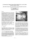
A Demonstrated Optical Tracker With Scalable Work Area for HeadMounted Display Systems
Mark Ward†, Ronald Azuma, Robert Bennett, Stefan Gottschalk, Henry Fuchs
Department of Computer Science
Sitterson Hall
University of North Carolina
Chapel Hill, NC 27599-3175
Abstract
An optoelectronic head-tracking system for head-mounted
displays is described. The system features a scalable work area
that currently measures 10' x 12', a measurement update rate of
20-100 Hz with 20-60 ms of delay, and a resolution
specification of 2 mm and 0.2 degrees. The sensors consist of
four head-mounted imaging devices that view infrared lightemitting diodes (LEDs) mounted in a 10' x 12' grid of modular 2'
x 2' suspended ceiling panels. Photogrammetric techniques
allow the head's location to be expressed as a function of the
known LED positions and their projected images on the
sensors. The work area is scaled by simply adding panels to
the ceiling's grid. Discontinuities that occurred when changing
working sets of LEDs were reduced by carefully managing all
error sources, including LED placement tolerances, and by
adopting an overdetermined mathematical model for the
computation of head position: space resection by collinearity.
The working system was demonstrated in the Tomorrow's
Realities gallery at the ACM SIGGRAPH '91 conference.
CR categories and subject descriptors: I.3.1
[Computer Graphics]: Hardware Architecture - t h r e e dimensional displays; I.3.7 [Computer Graphics]: ThreeDimensional Graphics and Realism - Virtual Reality
Additional Key Words and Phrases:
displays, head tracking
1
Head-mounted
Introduction
It is generally accepted that deficiencies in accuracy,
resolution, update rate, and lag in the measurement of head
position can adversely affect the overall performance of a HMD
[17][24][25]. Our experience suggests that an additional
specification requires more emphasis: range.
† Present address: Structural Acoustics, 5801 Lease Lane,
Raleigh, NC, 27613. (919) 787-0887
Figure 1: The existing system in UNC's graphics laboratory
Most existing HMD trackers were built to support situations
that do not require long-range tracking, such as cockpit-like
environments where the user is confined to a seat and the range
of head motion is limited.
But many virtual worlds
applications, such as architectural walkthroughs, would benefit
from more freedom of movement (Figure 2). Long-range
trackers would allow greater areas to be explored naturally, on
foot, reducing the need to resort to techniques such as flying or
walking on treadmills.
Such techniques of extending range work adequately with
closed-view HMDs that completely obscure reality. With seethrough HMDs [9][11], however, the user's visual connection
with reality is intact and hybrid applications are possible
where physical objects and computer-generated images coexist.
In this situation, flying though the model is meaningless. The
model is registered to the physical world and one's relationship
to both must change simultaneously.
This paper describes the second generation of an
optoelectronic head-tracking concept developed at the
University of North Carolina at Chapel Hill. In the concept's
first generation, the fundamental design parameters were
explored and a bench-top prototype was constructed [28].
Building on this success, the second-generation tracker is a
fully functional prototype that significantly extends the
workspace of an HMD wearer.
2
Previous work
Many tracking systems precede this effort, and we will briefly
survey representative examples. The essence of the problem is
the realtime measurement of the position and orientation of a
rigid moving body with respect to an absolute reference frame,
a six-degree-of-freedom (6DOF) measurement problem.
Solutions are relevant to many other fields.
To our knowledge, four fundamentally different technologies
have been used to track HMDs: mechanical, magnetic,
ultrasonic, and optical.
The first HMD, built by Ivan Sutherland [27], used a mechanical
linkage to measure head position. A commercial product, The
Boom [12], uses a mechanical linkage to measure the gaze
direction of a hand-held binocular display. The Air Force
Human Resources Laboratory (AFHRL) uses a mechanical
linkage to measure the position and orientation of a HMD used
for simulation [24]. Mechanical systems have sufficient
accuracy, resolution, and frequency response, yet their range is
severely limited, and a mechanical tether is undesirable for
many applications.
Figure 2: Walkthrough of Brooks' kitchen design that runs with
the tracker. Actual resolution of images seen in the HMD is
much lower than this picture's resolution.
The current system (Figure 1) places four outward-looking
image sensors on the wearer's head and locates LEDs in a 10' x
12' suspended ceiling structure of modular 2' x 2' ceiling
panels. Each panel houses 32 LEDs, for a total of 960 LEDs in
the ceiling. Images of LEDs are formed by lateral-effect
photodiode detectors within each head-mounted sensor. The
location of each LED's image on a detector, or
photocoordinate, is used along with the known LED locations
in the ceiling to compute the head's position and orientation.
To enhance resolution, the field of view of each sensor is
narrow. Thus, as shown in Figures 3 and 7, each sensor sees
only a small number of LEDs at any instant. As the user moves
about, the working set of visible LEDs changes, making this a
cellular head-tracking system.
Measurements of head position and orientation are produced at
a rate of 20-100 Hz with 20-60 ms of delay. The system's
accuracy has not been measured precisely, but the resolution is
2 mm and 0.2 degrees. It was demonstrated in the Tomorrow's
Realities gallery at the ACM SIGGRAPH '91 conference, and is,
to our knowledge, the first demonstrated scalable head-tracking
system for HMDs.
The system is novel for two reasons. First, the sensor
configuration is unique. Other optical tracking systems fix the
sensors in the environment and mount the LEDs on the moving
body [30]. The outward-looking configuration is superior for it
improves the system's ability to detect head rotation. The
scalable work space is the system's second contribution. If a
larger work space is desired, more panels can be easily added to
the overhead grid.
Magnetic-based systems [3][21] are the most widely used hand
and head trackers today.
They are small, relatively
inexpensive, and do not have line-of-sight restrictions. Their
primary limitations are distortions caused by metal or
electromagnetic fields, and limited range [13].
Ultrasonic approaches have also been successful, such as the
commercially-available Logitech tracker [20]. Time-of-flight
measurements are used to triangulate the positions of sensors
mounted on the HMD. The strength of this technology is
minimum helmet weight [13]. Physical obscuration as well as
reflections and variations of the speed of sound due to changes
in the ambient air density make it difficult to maintain accuracy
[5].
Because of the potential for operation over greater distances,
optical approaches are plentiful, and it is helpful to categorize
them on the basis of the light source used. Visible, infrared,
and laser light sources have each been exploited.
Ferrin [13] reports the existence of a prototype helmet tracking
system using visible light.
Although it only tracks
orientation, it is worth mentioning here because of its unique
approach. A patterned target is placed on the helmet and a
cockpit-mounted video camera acquires images in real time. The
pattern is designed to produce a unique image for any possible
head orientation. The strength of this approach is the use of
passive targets which minimize helmet weight. Reflections
and other light sources are potential sources of error.
Bishop's Self-Tracker [7] is a research effort involving visible
light. A Self-Tracker chip senses incremental displacements
and rotations by imaging an unstructured scene. A headmounted cluster of these chips provide sufficient information
for the computation of head position and orientation.
Although still under development, the concept is mentioned
here because it would allow an optical tracking system to
operate outdoors, where a structured environment, such as our
ceiling of LEDs, would be impossible to realize.
Because of the difficulties associated with processing
information in an unstructured scene, most high-speed optical
measurement systems use highly-structured infrared or laser
light sources in conjunction with solid-state sensors. The
sensor is a often a lateral-effect photodiode as opposed to a true
imaging device, because the photodiode produces currents that
are directly related to the location of a light spot's centroid on
its sensitive surface [32]. The resultant sensor is relatively
insensitive to focus, and the light spot's location, or
photocoordinate, is immediately available without the need for
image processing.
During the 1970's, Selspot [23] popularized the use of infrared
LEDs as targets and lateral-effect photodiodes as sensors in a
commercially-available system. Their primary emphasis was,
and still is, on the three-dimensional locations of individual
targets. That is, the Selspot system does not automate the
computation of a rigid body's orientation. In a response to this
shortcoming, Antonsson [2] refined the Selspot system for use
in dynamic measurements of mechanical systems. The
resultant system uses two Selspot cameras to view a moving
body instrumented with LEDs. Similar approaches have been
applied to HMD systems in cockpits [13] and in simulators
[11].
The use of an LED light source limits the range of these
systems. Typically, the distance between source and detector
can be no greater than several feet. Longer distances can be
spanned with laser light sources.
The only known example of a 6DOF tracker using laser sources
is the Minnesota Scanner [26]. With this sytem, scanning
mirrors are used to sweep orthogonal stripes of light across the
working volume. Photodiodes are both fixed in space and
placed on the moving body. By measuring the time between a
light stripe's contact with a fixed and moving photodiode, the
diode's three-dimensional location can be computed. Given the
location of three or more moving diodes, the moving body's
orientation can be computed. Similar technology has been
applied to the cockpit, although orientation was the only
concern [13].
3
System overview
Wang demonstrated the viability of head-mounted lateral-effect
photodiodes and overhead LEDs. This system extends his work
in several ways. First, an overhead grid of 960 LEDs was
produced with well-controlled LED location tolerances, and
more attention was paid to controlling other error sources as
well. Second, mathematical techniques were developed that
allow an arbitrary number of sensors and an arbitrary number of
LEDs in the field of view of each sensor to be used in the
computation of head location.
This resulted in an
overdetermined system of equations which, when solved, was
less susceptible to system error sources than the previous
mathematical approach [10]. Third, the analog signals
emerging from the sensors were digitally processed to reject
ambient light. Finally, techniques for quickly determining the
working sets of LEDs were developed.
3.1 Sensor configuration
Typically, optical trackers are inward-looking; sensors are
fixed in the environment within which the HMD wearer moves.
With Self-Tracker, Bishop and Fuchs introduced the concept of
outward-looking trackers that mount the image sensors on the
head, looking out at the environment (Figure 3).
If a large work area is required, outward-looking configurations
have an advantage over inward-looking techniques when
recovering orientation. The two are equivalent for measuring
translation: moving the sensor causes the same image shift as
moving the scene. Rotations are significantly different.
Unless targets are mounted on antlers, an inward-looking
sensor perceives a small image shift when the user performs a
small head rotation. The same head rotation creates a much
larger image shift with a head-mounted sensor. For a given
sensor resolution, an outward-looking system is more
sensitive to orientation changes.
Figure 4: Remote Processor and head unit with four sensors
To improve resolution in general, long focal lengths must be
used with an optical sensor regardless of whether the
configuration is inward or outward-looking. Thus, a wide-angle
lens cannot significantly extend the work area of an inwardlooking system without sacrificing resolution and accuracy.
Figure 3: Conceptual drawing of outward-looking system and
the sensors' fields of view
Narrow fields of view are a consequence of long focal lengths.
Therefore, the HMD wearer cannot move very far before an LED
leaves a given sensor's field of view. One solution is a cellular
array of either LEDs or detectors. For an infrared system using
LEDs and lateral-effect photodiodes, system cost is minimized
by replicating LEDs as opposed to sensors. This is a result of
both the device cost as well as the required support circuitry.
In the current system, four Hamamatsu (model S1880) sensors
are mounted atop the head, as shown in Figure 4. Each sensor
consists of a camera body to which a Fujinon lens (model CF
50B) is attached. The focal length of each lens is 50mm. Their
principal points were determined experimentally by an optical
laboratory. An infrared filter (Tiffen 87) is used to reject
ambient light.
The LED Manager is a 68030-based processing module that
controls the Remote Processor as well as the ceiling. A TAXIbased serial datalink [1] provides access to the Remote
Processor while the ceiling's data daisy chain terminates at the
LED Manager. Software executing on this module is
responsible for turning LEDs on and for extracting data from
the sensors. The LED Manager resides in a remote VME chassis
that must be located near the ceiling structure.
3.2 Beacon configuration
Experience with simulations and an early 48-LED prototype
revealed the problem of beacon switching error: as the user
moved around and the working set of beacons changed,
discontinuous jumps in position and orientation occurred.
These are caused by errors in the sensor locations, distortions
caused by the lens and photodiode detector, and errors in the
positions of the beacons in the ceiling.
To control beacon locations, we housed the LEDs in carefully
constructed ceiling panels. Each 2' x 2' panel is an anodized
aluminum enclosure that encases a 20" x 20" two-sided printed
circuit board. On this board are electronics to drive 32 LEDs.
The LEDs are mounted in the front surface with standard plastic
insets. Using standard electronic enclosure manufacturing
techniques, it was relatively easy to realize an LED-to-LED
centerline spacing tolerance of .005" on a given panel.
The panels are hung from a Unistrut superstructure (Figure 1).
At each interior vertex of a 2' x 2' grid, a vertically adjustable
hanger mates with four panels. Four holes in the face of a panel
slide onto one of four dowels on each hanger. The entire array
of panels is levelled with a Spectra Physics Laser-Level, which
establishes a plane of visible red light several inches below the
panels' faces. Each hanger is designed to accept a sensor
(Industra-Eye) that measures the vertical position of the laser
relative to its own case. By moving the hangers up or down,
they can be aligned to within .006" of the light beam.
The panels are electrically connected by a data and power daisy
chain. The data daisy chain allows an individual LED to be
selected. Once selected, the LED (Siemens SFH 487P) can be
driven with a programmable current that ranges from 0-2
amperes. The programmable current allows an electronic iris
feature to be implemented. Typically, an LED will be on for no
more than 200 µsec. During this time period, the current is
adjusted to achieve a desired signal level at the sensor (see
Section 4).
3.3 Data Flow
As shown in Figure 5, the signals emerging from the headmounted sensors are connected to the Remote Processor. Worn
as a belt pack, the Remote Processor functions as a remote
analog-to-digital conversion module. It can accept the four
analog voltages emerging from a lateral-effect photodiode, for
up to eight sensors. On command, the Remote Processor will
simultaneously sample the four voltages on a selected sensor
and relay four, 12-bit results to the LED Manager. The Remote
Processor was used to alleviate the need for long runs of analog
signals emerging from multiple sensors.
Figure 5: System Dataflow
For each measurement of head location, the LED Manager
produces a list of visible LEDs and their associated
photocoordinates. This list is transferred via shared memory to
the Collinearity module, which resides in the graphics engine's
VME chassis. The i860-based Collinearity module translates
the list of photocoordinates into the current estimate of head
location. For reasons explained in Section 6, an additional
68030-based processor is used to aid the transfer of data from
the remote system to the host. In theory, this is not required.
The VME systems are connected by a Bit-3 VME buslink.
The sampled head position is communicated to the Pixel-Planes
5 graphics engine [14], which in turn updates the images on the
user's displays.
4
Low-level software
A library of low-level routines running on the LED Manager,
called the Acquisition Manager, controls the beacons and
detectors. Given an LED and a photodiode unit, these routines
light an LED and determine if a photodiode's detector sees that
LED. The detector returns four analog signals, which the
Remote Processor board digitizes. A simple formula [16]
converts these four numbers into the x,y photocoordinates of
the LED's projection on the detector.
Hamamatsu datasheets specify 1 part in 40 accuracy and 1 part
in 5000 resolution for the lateral-effect diode-based detectors
used. As with Antonsson [2], we were able to achieve
approximately 1 part in 1000 accuracy for the combined
photodiode-lens assembly. Achieving this result required
significant efforts to improve the signal-to-noise ratio and
compensate for distortion, including:
100 µsec. LEDs are tested in groups; each group carries an
additional overhead of 60 µsec.
Ambient light rejection: The voltage values with the LED off
(called the "dark current") are subtracted from the voltage values
with the LED on. Sampling with the LED off both before and
after the samples with the LED on and averaging the two yields
substantially improved ambient light rejection.
Random noise rejection: Averaging several measurements
reduces random noise effects, but costs time. A good
compromise between accuracy and sampling speed is to take 8
samples with the LED off, 16 samples with the LED on and 8
more samples with the LED off.
Current scaling: The distance between a photodiode and an LED
depends on the user's location. To maximize the signal without
saturating the photodiode detector, the Acquisition Manager
dynamically adjusts the amount of current used to light an LED.
Acquisition Manager routines estimate the threshold of current
that will saturate the detector and use 90% of this value during
sampling.
Figure 7: Sensors viewing LEDs in the ceiling. Each of the four
groups is the set of LEDs that a sensor can see. Picture taken
with a camera that is sensitive to infrared light.
5
LED Manager
The LED Manager uses the low-level Acquisition Manager
routines to determine which LEDs each photodiode unit sees
and where the associated imaged points are on the photodiode
detectors. We usually want to collect data from all visible
LEDs, since larger sample sets ultimately yield less noisy
solutions from the Collinearity module (Section 7). Because
the number of visible LEDs is small (see Figure 7) compared to
the total number of LEDs in the ceiling, something faster than
a brute-force scan of the entire ceiling array is called for. Two
assumptions help us design a more efficient method:
1) Spatial coherence: The set of beacons visible to a
photodiode unit in a given frame will be contiguous.
Figure 6: Optical bench for photodiode calibration
Calibration: Both the lens and the photodiode detector suffer
from nonlinear distortions. By placing the photodiodes on an
optical bench and carefully measuring the imaged points
generated by beacons at known locations (Figure 6), we built a
lookup table to compensate for these distortions. Bilinear
interpolation provides complete coverage across the detector.
More sophisticated calibration techniques should be
investigated. Accurate calibration is required to reduce beacon
switching error.
Programming techniques: Techniques such as list processing,
cache management and efficient code sequencing result in a
substantially improved sampling rate. In addition, expedited
handling of special cases, such as when an LED is not within
the field of view of a photodiode unit, further helps system
performance.
Using 32 samples per LED, we compute a visible LED's
photocoordinate in 660 µsec and reject a non-visible LED in
2) Temporal coherence: The user's movement rate will be slow
compared to the frame rate. This implies that the field of view
of a given photodiode unit does not travel very far across the
ceiling between frames, so its set of visible beacons will not
change much from one frame to the next.
5.1
The basic method
In each frame, the LED Manager goes through each photodiode
unit in sequence, sampling beacons until it is satisfied that it
has captured most of each photodiode unit's visible set. A
basic difficulty is that we cannot be sure whether a beacon is
visible or not until we attempt to sample it. The LED Manager
remembers which beacons were in the camera's visible set from
the previous frame. The set is called the last visible set. If the
last visible set is nonempty, all beacons in that set are tested.
The next action depends on how many of those beacons are
actually visible:
1) All: We assume the field of view has not moved much and
not many more beacons will be visible. We stop with this set
and go on to the next photodiode unit.
2) Some: We assume that the field of view has shifted
significantly, possibly enough to include previously unseen
beacons. A shell fill (described later) is conducted, beginning
with the set of beacons verified to be visible.
3) None: The field of view has moved dramatically, gone off
the edge of the ceiling, or is obscured. We check the neighbors
of the last visible set. If any of these beacons are visible, they
are used to start a shell fill. If none are visible, we give up on
this photodiode unit until the next frame.
What if the last visible set is empty? Our course of action
depends on whether we were able to compute a valid position
and orientation for the head in the last frame:
1) Valid previous location: We can predict which LEDs should
be visible to our photodiode unit, if the user's head is actually
at the computed location, because the geometry of the head unit
is known. If no LEDs are predicted to be visible, we go on to
the next photodiode unit, otherwise we sample those beacons
and use them as the start of a shell fill, if any of them were
actually visible.
2) No valid previous location: Now we have no way to guess
which beacons are visible, so we resort to a simple sweep
search, which lights the beacons in the ceiling row by row,
until we have tried the entire ceiling or an LED is found to be
visible. In the former case, we give up, and in the latter case,
we use the visible beacon as the start of a shell fill.
The queuing mechanism lets all modules in the system run
asynchronously. LED Manager, the Collinearity module, and
Pixel-Planes 5 run as fast as they can, using the most recent
data in the queue or the last known data if the queue is empty.
The various processors in our system are split between two
separate VME buses, which are transparently linked together
by Bit-3 bus link adapters (Figure 5). A subtle bus loading
problem prevents the i860 board and the '030 board that runs
LED Manager from operating in the same VME cage. This
configuration increases latency because inter-bus access is
significantly slower than intra-bus access, but increases
throughput because the bus link allows simultaneous intra-bus
activity to occur. Because the i860 processor cannot directly
access the VME bus, a second '030 board, which runs the Queue
Manager, moves data between the LED Manager and the
Collinearity module.
A simpler and less expensive system could be built if we
acquired an i860 board that can run on the same bus as the LED
Manager '030 board. This configuration would not require the
Queue Manager board or the Bit-3 links and would reduce both
latency and throughput.
7
5.2
Shell fill
A shell fill starts with a set of beacons known to be visible to a
sensor and sweeps outward until it has found all the beacons in
the field of view.
We do this by first sampling the neighbors of the initial set of
beacons. If none are found visible, the shell fill terminates,
concluding that the beacons in the initial set are the only
visible ones. If any are found visible, we then compute the
neighbors of the beacons we just sampled, excluding those
which have already been tried, and sample those. We repeat
this process of sampling beacons, computing the neighbors of
those found visible, and using those neighbors as the next
sample set, until an iteration yields no additional visible
beacons.
Space Resection by Collinearity
Given the observations of beacons, we compute the position
and orientation of the user's head by using a photogrammetric
technique called space resection by collinearity. The basic
method for a single camera is in [31]; what we describe here is
our extension for using it in a multi-sensor system. Because of
space limitations, the description is necessarily brief. Full
details are provided in [6].
7.1 Definitions
Three types of coordinate systems exist: one World space (tied
to the ceiling structure), one Head space (tied to the HMD), and
several Photodiode spaces (one for each photodiode unit).
Assumption 1, that visible sets are contiguous, suggests that
this procedure should be thorough and reasonably efficient.
5.3
Startup
At startup, the head location is not known and all of the last
visible sets are empty. We do a sweep search, as previously
described, for each photodiode unit to locate the initial visible
sets.
6
Communications
Communication between the various processors in our system
is done using shared memory buffers, which offer low latency
and high speed. The buffers are allocated and deallocated via a
FIFO queue mechanism. Data is "transmitted" when it is written
to the buffer: no copying is necessary.
The only
communication overhead is the execution of a simple
semaphore acquisition and pointer management routine.
Furthermore, all processors use the same byte ordering and data
type size, so no data translation is needed.
Photodiode
unit #1
Photodiode
unit #2
HEAD
WORLD
Figure 8: World, Head and Photodiode spaces
Changing representations from one space to another is done by
a rotation followed by a translation. We use two types of 3x3
rotation matrices:
M = Head space to World space
Mi = Photodiode space i to Head space
with each matrix specified by Euler angles ω , α, and κ.
LED j
X j , Y j , Zj
The optical model for each photodiode unit is simple: a light
ray strikes the front principal point and leaves the rear
principal point at the same angle (Figure 9).
Front
principal
point
Tij
LED
j
WORLD
X 0, Y 0, Z0
e
Imaged
point
fi
d
io
od
ot i
Ph it
un
Rear principal
point
HEAD
ø
ø
Front
principal
point
-Tij
Figure 10: Expressing Tij through other vectors
tij
Imaged
point
Detector
Dete
ctor
Photodiode unit i
Figure 9: Optical model
-tij
HEAD
Finally, we list the points and vectors we will need, segregated
by the coordinate system in which they are represented. Given
photodiode unit i sees LED number j,
ei
x ij , y ij , 0
di
de
odio
Phot
i
unit
Figure 11: Expressing tij through other vectors
Photodiode space:
[xij, yij, 0] = imaged point on photodiode detector
Rear principal
point
Head space:
tij = vector from rear principal point to imaged point
H0 = origin of Head space
di = vector from H0 to center of photodiode detector
ei = vector from H 0 to rear principal point
fi = vector from H 0 to front principal point
Substituting (2) and (3) into (1) yields the collinearity
condition equation cij :
World space:
[X0, Y0, Z0] = coordinates of the origin of Head space
[Xj, Yj, Zj] = coordinates of LED j
Tij = vector from LED j to front principal point
7.3 System of equations
When a photodiode unit i sees an LED j, it generates a cij, which
represents three independent equations. If we see N LEDs in all,
the total number of unknowns in our system is 6+N : 3 for
position, 3 for orientation, and N scale factors. The first six
are what we are trying to find, but we do not care about the scale
factors. We eliminate these by rearranging the c ij equations,
then dividing the first and second equations by the third. This
leaves two independent equations, of the form
7.2 Geometric relationships
Figure 9 shows that T ij and t ij differ only by a scale factor; if
they were placed at the same start point, they would be
collinear. In equations:
(1)
Tij = λ M tij
We now express Tij and tij in terms of the other vectors in
equations (2) and (3) and Figures 10 and 11:
T ij =
X0 - Xj
Y0 - Yj
Z0 - Z j
+ M fi
xij
tij = di - ei + M i y i j
0
cij:
X0 - Xj
Y0 - Yj
Z0 - Zj
G1ij(L) = 0, G2ij(L) = 0
where L is a vector composed of the six unknowns: position
(X 0 , Y 0 , Z 0 ) and orientation (ω , α , κ for matrix M ). We
generate a linear approximation to these two equations by
applying Taylor’s theorem:
(2)
-G1ij(L) =
(3)
xij
+ M f i = λ M di - ei + M i y i j
0
+
∂G1ij(L)
∂X 0
∂G1ij(L)
dX0 +
∂G1ij(L)
∂Y 0
∂G1ij(L)
dY0 +
∂G1ij(L)
dZ0
∂Z0
∂G1ij(L)
dω +
dα +
dκ
∂ω
∂α
∂κ
and a similar expansion for the linearized G2 equation.
Now we have six total unknowns, and every LED that we see
generates two independent linear equations. Thus, we need to
see at least three LEDs. If we see a total of N LEDs, we can write
our system of N linearized G1 equations and N linearized G 2
equations in matrix form:
-G0 = ∂G * D
2Nx1 2Nx6 6x1
(4)
where D = [dX0, dY0, dZ0, dω, dα, dκ]T,
∂G is the matrix of partial derivatives of the G1 and G2,
and -G0 contains the values of the G1 and G2 at a specific L.
7.4 Iteration and convergence
Collinearity takes an initial guess of L (the unknowns) and
generates correction values (in D) to make a more accurate L,
iterating until it converges to a solution. Thus, we need to
extract D from equation (4). If N = 3, then we can solve for D
directly. If N > 3, then the system is overdetermined and we
approximate D through singular value decomposition [24].
Simulations show that using more than the minimum of 3 LEDs
can reduce average error caused by non-systematic error
sources. In pseudocode, our main loop is:
Generate an initial guess for L
repeat
Given L, compute G0 and ∂G
Estimate D using singular value decomposition
L=L+D
until magnitude of D is small
return L
How do we generate the initial guess of L? Normally we use the
last known position and orientation, which should be an
excellent guess because we track at rates up to 100 Hz.
Collinearity usually converges in 1 or 2 iterations when the
guess is close. But in degenerate cases (at system startup, or
when we lose tracking because the photodiode units are pointed
away from the ceiling), we have no previous L. Collinearity
will not converge if the guess is not close enough to the true
value; we empirically found that being within 30o and several
feet of the true L is a good rule of thumb. So in degenerate
cases, we draw initial guesses for L from a precomputed lookup
table with 120 entries, trying them sequentially until one
converges. We can double-check a result that converges by
comparing the set of LEDs used to generate that solution to the
theoretical set of LEDs that the photodiode units should see, if
the head actually was at the location just computed. When
these two sets match, we have a valid solution.
8
Performance
A "typical situation" is defined as a user of average height
standing erect underneath the ceiling, with at least three
photodiode units aimed at the ceiling, moving his head at
moderate speeds. All measurement bounds assume that the user
remains in tracker range with at least two sensors aimed at the
ceiling.
Update rate: The update rate ranges between 20–100 Hz. Under
typical situations, 50-70 Hz is normal, depending on the
height of the user. The wide variation in the number of LEDs
seen by the sensors causes the variation in update rate. The
more LEDs used, the slower the update rate, because LED
Manager is the slowest step in the pipeline. If the head
remains still and the sensors see a total of B beacons, LED
Manager requires 3.33 + 0.782*B ms to run. Rapidly rotating
the head increases this time by a factor of about 1.33, since
additional time is required to handle the changing working sets
of LEDs. Slower head movement rates have correspondingly
smaller factors.
Lag: Lag varies between 20–60 ms, with 30 ms being normal
under typical situations. Lag is measured from the time that
LED Manager starts to the time when the Collinearity module
provides a computed head location to the graphics engine.
Therefore, tracker latency is a function of the number of LEDs
seen and the quality of the initial guess provided to the
Collinearity module. As B gets smaller, both the LED Manager
and Collinearity modules become faster, reducing latency. This
mutual dependence on B means that update rate and lag are
closely tied: faster update rates correspond with lower latency
values.
Resolution: When moving the head unit very slowly, we
observed a resolution of 2 mm in position and 0.2 degrees in
orientation. Measuring accuracy is much harder, and we do not
have any firm numbers for that yet. At SIGGRAPH '91, users
were able to touch a chair and the four ceiling support poles
based solely on the images they saw of models of the chair and
the poles in the virtual environment.
9
Evaluation
The system provides adequate performance but has several
limitations and problems that must be addressed. The most
noticeable is the combination of excessive head-born weight
and limited head rotation range. Rotation range depends
heavily on the user's height and position under the ceiling. A
typical maximum pitch range near the center of the ceiling is
45 degrees forward and 45 degrees back. When the user walks
near an edge of the ceiling, head rotation range becomes much
more restricted. To accommodate the full range of head motion,
multiple image sensors must be oriented such that wherever the
head is pointed, two or more sensors are able to view LEDs on
the ceiling. Given the current focal lengths, simulations show
that as many as eight fields of view are required for a
respectable rotation range [29]. The weight of each sensor
must be significantly reduced to achieve this goal.
To reduce weight, we are trying to replace the current lenses (11
oz. each) with smaller, lighter lenses (2 oz. each). Other
approaches are possible.
Wang proposed optically
multiplexing multiple fields of view onto on a single lateraleffect photodiode [29]. Reduced signal strength, distortions,
and view identification ambiguities make this a nontrivial
task. It may be easier to design a helmet with integral
photodiodes and lenses. Given that each photodiode is about
the size of a quarter, the entire surface of a helmet could be
studded with sensors.
Beacon switching error has been greatly reduced, but not
eliminated. Small observable discontinuities occasionally
occur, and while they are not a major disturbance, they are
annoying. Calibration techniques are being explored to
estimate error sources and compensate for their effects.
Photogrammetric techniques like the bundle adjustment method
[8] or an alternate scheme suggested by our colleagues [18] may
provide the answer.
Infrared light sources in the environment surrounding the
tracker, such as sunlight or incandescent light, must be
controlled for the system to operate correctly. Specifically,
any light source whose wavelengths include 880 nm will be
detected by the photodiodes as if it were an LED. For this
reason, fluorescent ambient lighting is preferred. Extreme
caution is not required, however. Whereas a sensor pointed
directly at an infrared light source other than the LEDs will
confuse the system, a certain level of indirect infrared
background light is tolerable due to the combination of optical
filters and the ambient light rejection techniques described in
Section 4.
Surprisingly, the bottleneck in the system is the time required
to extract data from the photodiode detectors, not the time
required to compute the head's location. The i860 processor
performs the latter task adequately, and even faster and cheaper
processors will be available in the future. But getting accurate
photocoordinates from the detectors takes longer than
expected, because of the time spent in current scaling and in
sampling multiple times per LED. Further experimentation is
required to see if we can safely reduce the number of samples.
Optimizing the low-level software may improve sampling
speed by 20-30%.
The use of Euler angles in the collinearity equations opens the
possibility of gimbal lock. The current system avoids this
because the head rotation range is too limited to reach gimbal
lock positions, but a future version may. If we cannot place the
gimbal lock positions out of reach, we can solve for the nine
rotation matrix parameters individually, subject to six
constraints that keep the matrix special orthogonal, or we may
be able to recast the rotations as quaternions.
Since this tracker encourages the user to walk around large
spaces, tripping over the supporting cables is a danger. We
will investigate the feasibility of a wireless datalink to remove
this problem.
Under certain circumstances, the sensors can see large numbers
of beacons, such as a total of 30 or more. While using many
LEDs usually improves the solution from the Collinearity
module, it also slows down the update rate and increases the
lag. Further experiments are needed to explore this tradeoff and
determine rules of thumb that provide a reasonable balance
between resolution and update rate.
Cellular systems using different technologies or configurations
could be built to achieve similar scalable work areas. For
example, Ascension has announced a cellular magnetic system
[4]. Regardless of the technology, any cellular approach
creates the problem of beacon switching error or its equivalent.
Steps we took to control these errors would apply to other
technologies as well: 1) precise positioning and measurement
of system components, 2) averaging techniques to reduce
random error sources, and 3) calibration routines to compensate
for systematic error sources.
10
Future work
We intend to continue improving this system. In addition to
the tasks listed in Section 9, we would eventually like to
expand the ceiling size to around 20’ x 20’, to provide much
greater range of movement, both quantitatively and
psychologically. Also, ample room exists to improve the
heuristics and optimize the code, increasing the update rate and
reducing latency.
But beyond these incremental improvements, we do not expect
to pursue this particular technology further. The system is a
vehicle for further research and provides room-sized tracking
capability today for HMD applications that require it. For
example, the UNC Walkthrough team has begun interviewbased user studies on what impact large-environment tracking
has on the architectural design of a kitchen. In the future,
emphasis will be placed on technologies that allow unlimited
tracking volumes in unstructured environments. This potential
exists in systems that measure only the relative differences in
position and orientation as the user moves, integrating these
differences over time to recover the user's location. Examples
include inertial technologies and Self-Tracker. Since these
technologies suffer from drift problems, initial versions may
be hybrid systems reliant on the optical tracker for auxiliary
information. Thus, the optical tracking system will serve as a
testbed for its own successor.
Tracking HMDs will only get harder in the future. The higher
resolution displays being developed demand higher resolution
trackers. See-through HMDs add additional requirements. In
the completely-enclosed HMDs commonly used today, the
entire world is virtual, so resolution is much more important
than accuracy. But for a see-through HMD, accurate
registration of the HMD to the real world is vital. The effects
of latency will also become more disturbing in see-through
HMDs. Viewing computer-generated objects superimposed
upon the real world, where those objects move with significant
lag but the real world does not, will not provide a convincing
illusion. People can perceive as little as 5 ms of lag [15], and
it is unlikely that the combined tracker and graphics engine
latency will be below that anytime soon.
Therefore,
compensation techniques need to be explored [19][24]. If
HMDs are to achieve their potential of making a user truly feel
immersed inside a virtual world, significant advances in
tracking technologies must occur.
References
[1]
Advanced Micro Devices, Am7968/Am7969 TAXIchip
Article Reprints, Sunnyvale, CA.
[2]
Antonsson, E. K., and R.W. Mann. Automatic 6-D.O.F.
kinematic trajectory acquisition and analysis.
J.
Dynamic Systems, Measurement, and Control, 111,
(March 1989) pp. 31–39.
[3]
Ascension Technology Corporation. The Bird 6D Input
Device, Burlington, Vermont, 1989.
[4]
Ascension Technology Corporation. A Flock of Birds
product description sheet, Burlington, Vermont, April
1991.
[5]
Axt, Walter E. Evaluation of a pilot's line-of-sight using
ultrasonic measurements and a helmet mounted display.
Proceedings IEEE National Aerospace and Electronics
Conf. (Dayton, OH, May 18-22, 1987) pp. 921-927.
[6]
[7]
Azuma, Ronald, and Mark Ward. Space-resection by
collinearity: mathematics behind the optical ceiling
head-tracker. UNC Chapel Hill Dept. of Computer
Science technical report TR 91-048, Nov. 1991.
Bishop, Gary and Henry Fuchs. The self-tracker: A smart
optical sensor on silicon. Proceedings of the 1984 MIT
Conference on Advanced Research on VLSI (Dedham,
MA: Artech House, Jan 1984) pp. 65-73.
[23] SELCOM. SELSPOT II HARDWARE and MULTILab
Software, Southfield, Michigan, 1988.
[24] Smith Jr., B. R. Digital head tracking and position
prediction for helmet mounted visual display systems.
Proceedings of AIAA 22nd Aerospace Sciences Meeting,
(Reno, NV, Jan. 9-12, 1984).
[8]
Burnside, C. D. Mapping from Aerial Photographs.
Granada Publishing Limited, G. Britain, 1979, pp. 248258.
[25] So, Richard H., and Michael J. Griffin. Effects of time
delays on head tracking performance and the benefits of
lag compensation by image deflection. Proceedings of
AIAA Flight Simulation Technologies Conference (New
Orleans, LA, Aug. 12-14, 1991) pp. 124-130.
[9]
Chung, Jim, Mark Harris, Fred Brooks, et al. Exploring
Virtual Worlds with Head-Mounted Displays. SPIE
Proceedings vol. 1083 Non-Holographic True 3Dimensional Display Technologies (Los Angeles, CA,
Jan 15-20, 1989).
[26] Sorensen, Brett, Max Donath, Guo-Ben Yang, and Roland
Starr. The Minnesota scanner: a prototype sensor for
three-dimensional tracking of moving body segments.
IEEE Transactions on Robotics and Automation, 5, 4,
(August 1989), pp. 499–509.
[10] Church, Earl. Revised geometry of the aerial photograph.
Bulletins on Aerial Photogrammetry, No. 15, Syracuse
University, 1945.
[27] Sutherland, Ivan. A head-mounted three dimensional
display. Fall Joint Computer Conference, AFIPS
Conference Proceedings, 33 (1968) pp. 757-764.
[11] Cook, Anthony. The helmet-mounted visual system in
flight simulation. Proceedings Flight simulation: Recent
developments in technology and use. (Royal
Aeronautical Society, London, England, Apr. 12-13,
1988) pp. 214-232.
[28] Wang, Jih-Fang, Vernon Chi, and Henry Fuchs. A realtime 6D optical tracker for head-mounted display
systems. Proceedings of 1990 Symposium on Interactive
3D Graphics (Snowbird, Utah, 1990). In C o m p u t e r
Graphics 24, 2 (March 1990) pp. 205-215.
[12] Fake Space Labs, Binocular Omni-Orientation Monitor
(BOOM), Menlo Park, CA.
[29] Wang, Jih-Fang, Ronald Azuma, Gary Bishop, Vernon
Chi, John Eyles, Henry Fuchs. Tracking a head-mounted
display in a room-sized environment with head-mounted
cameras. SPIE Proceedings Vol. 1290 Helmet-Mounted
Displays II (Orlando, FL, Apr 19-20 1990) pp. 47-57.
[13] Ferrin, Frank J. Survey of helmet tracking technologies.
SPIE Vol. 1456 Large-Screen Projection, Avionic, and
Helmet-Mounted Displays (1991) pp. 86-94.
[14] Fuchs, Henry, John Poulton, John Eyles, et. al. PixelPlanes 5: A Heterogeneous Multiprocessor Graphics
System Using Processor-Enhanced Memories.
Proceedings of SIGGRAPH ‘89 (Boston, MA, July 31Aug 4, 1989). In Computer Graphics 23, 3 (July 1989)
pp. 79-88.
[30] Welch, Brian, Ron Kruk, Jean Baribeau, et al. Flight
Simulator: Wide-Field-Of-View Helmet-Mounted Infinity
Display System, Air Force Human Resources Laboratory
technical report AFHRL-TR-85-59, May 1986, pp. 4860.
Personal
[31] Wolf, Paul. Elements of Photogrammetry, With Air
Photo Interpretation and Remote Sensing, 2nd ed.,
McGraw-Hill, New York, 1983.
[16] Hamamatsu. Hamamatsu Photonics, Hamamatsu City,
Japan, 1985.
[32] Woltring, Herman. Single- and Dual-Axis Lateral
Photodetectors of Rectangular Shape. IEEE Trans. on
Electron Devices, (August 1975) pp. 581–590.
[15] Furness, Tom,
communication.
and
Gary
Bishop.
[17] Hardyman, G. M. and M. H. Smith. Helmet mounted
display applications for enhanced pilot awareness.
Proceedings of AIAA Flight Simulation Technologies
Conference (Boston, MA, Aug. 14-16, 1989) pp. 221225.
[18] Hughes, John F., and Al Barr. Personal communication.
[19] Liang, Jiandong, Chris Shaw, Mark Green. On TemporalSpatial Realism in the Virtual Reality Environment.
Proceedings of the 4th annual ACM Symposium on User
Interface Software & Technology (Hilton Head, SC, Nov
11-13 1991) pp. 19-25.
[20] Logitech, Inc. Logitech 3-D Mouse news release. July
30, 1991.
[21] POLHEMUS 3SPACE User's Manual, OPM3016-004B,
Colchester, Vermont, 1987.
[22] Press, William, Brian Flannery, Saul Teukolsky, William
Vetterling. Numerical Recipes in C. Cambridge
University Press, USA, 1988.
Acknowledgements
This system would not exist today without the support of the
Microelectronics System Laboratory, the Graphics Laboratory
staff, and the other members of the Tracker group. The authors
wish to thank Gary Bishop, Vern Chi, Carney Clegg, John
Eyles, David Harrison, John Hughes, Jack Kite, Mark Mine,
John Poulton, C. A. Stone, John Thomas, and Norm Vogel for
all of their help. We also thank Fred Brooks and the UNC
Walkthrough group for providing architectural applications to
use with our tracker.
Accu-Tool Corporation of Cary, NC was responsible for the
head frame's design and fabrication. Panel enclosures were
fabricated by Southeastern Machine Tool of Raleigh, NC. All
circuit boards were fabricated by Multilayer Technologies, Inc.
of Irvine, CA. This work was partially supported by ONR
contract N00014-86-K-0680, DARPA contract DAEA 18-90-C0044, NSF contract ASC-8920219, and a Pogue Fellowship.