Download RDSAT 5.6 User Manual - Respondent Driven Sampling

RDS INCORPORATED
RDS Analysis
Tool v5.6
User Manual
RDS INC.
RDSAT 5.6 User Manual
 RDS Incorporated
45 Beckett Way
Ithaca, NY 14850
(607) 255-4368
Publication Date: December 6, 2006
Table of Contents
Installing the RDS Analysis Tool v5.6 ....................................... 1
Basic Layout Information........................................................... 2
Preparing Data from Excel ........................................................ 3
Preparing Data from SPSS ....................................................... 6
Preparing data from SAS ........................................................ 10
Preparing Data from the RDS Coupon Manager..................... 11
Loading Data ........................................................................... 13
Viewing Data ........................................................................... 15
Setting Options For Analysis ................................................... 17
Adjust Average Network Sizes...................................................... 17
Number of Re-samples ................................................................. 17
Confidence Interval ....................................................................... 18
Pull-In Outliers of Network Sizes................................................... 18
Algorithm Type.............................................................................. 18
Partition Analysis..................................................................... 19
Data Parsing Options .............................................................. 20
Complete....................................................................................... 20
Breakpoint..................................................................................... 21
Analyze Continuous Variable ........................................................ 21
Custom.......................................................................................... 21
Breakpoint Analysis................................................................. 22
Interpreting a Partition Analysis............................................... 24
Recruitment ............................................................................. 25
Key of Group and Trait Correspondence ...................................... 26
Recruitments................................................................................. 26
Transition probabilities .................................................................. 26
Sample population sizes ............................................................... 27
Initial Recruits ............................................................................... 27
Estimation................................................................................ 28
Network Sizes and Homophily ................................................ 31
Adjusted Average Network Sizes .................................................. 31
Unadjusted Network Sizes ............................................................ 31
Network Size Information .............................................................. 32
Homophily ..................................................................................... 32
Affiliation Matrix............................................................................. 32
Graphics and Histograms........................................................ 32
Transition Probabilities.................................................................. 33
Degree List.................................................................................... 35
Bootstrap Simulation Results ........................................................ 35
Degree Distributions...................................................................... 36
Interpreting a Breakpoint Analysis........................................... 37
Replace Missing Data ............................................................. 40
Impute Median Values............................................................. 41
Impute Degree......................................................................... 42
Add Field Sample Weights ...................................................... 42
Estimate Number of Waves Required ..................................... 44
Save RDS Analysis in the File menu....................................... 46
Estimate Prevalence ............................................................... 46
RDS Analysis Tool File Menu Features .................................. 50
New RDS ...................................................................................... 50
View/Edit RDS .............................................................................. 50
Save RDS Analysis ....................................................................... 50
Print… ........................................................................................... 50
Export DL Network File ................................................................. 50
Export Population Weights............................................................ 51
Export Individualized Weights ....................................................... 51
Export Estimation Table ................................................................ 51
Export Table of Recruitments........................................................ 52
Options.......................................................................................... 52
Exit ................................................................................................ 52
RDS Glossary of Terms .......................................................... 53
Appendix 1: The RDS Data File .............................................. 58
Appendix 2: RDSAT Questions & Answers............................. 59
Appendix 3: Graphing Recruitment Chains with NETDraw ..... 61
The DL File: ............................................................................................ 61
The Attribute File: ................................................................................... 62
R D S
1
Chapter
I N C O R P O R A T E D
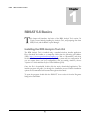
RDSAT 5.6 Basics
T
his chapter will introduce the basics of the RDS Analysis Tool version 5.6.
Topics covered include installing the Analysis Tool, and preparing data from
SPSS, Excel, and the RDS Coupon Manager.
Installing the RDS Analysis Tool v5.6
The RDS Analysis Tool is installed using a standard windows installer application.
First, download the installer to a temporary folder from the following web address
(URL): http://www.respondentdrivensampling.org. Click on “Downloads” and select
the download that matches your particular operating system and java configuration. If
you are unsure about your java configuration, and are running windows, choose
“Option #2” which includes the Java Virtual Machine (JVM).
Once the file is downloaded, double click the newly downloaded application: The
installer program will guide you through the installation process. Default installation
options are recommended and assumed throughout this manual.
To open the program, double click the “RDSAT” icon or select it from the Programs
listing in the Start Menu.
1
R D S
I N C O R P O R A T E D
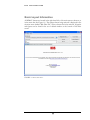
Basic Layout Information
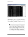
All RDSAT features are located in the right-hand side of the main screen as buttons, or
in the menu bar (See Figure 1.1). The current dataset being analyzed is displayed in the
selection menu entitled “Rds Data File.” When a dataset has been analyzed, all graphs
and figures can be found in the set of tabbed windows at the bottom of the main
screen.
FIGURE 1.1
RDSAT Main Window..
2
R D S
I N C O R P O R A T E D
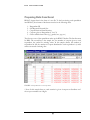
Preparing Data from Excel
RDSAT Accepts data in the form of a text file. To load an existing excel spreadsheet
into RDSAT, the columns of the dataset must be in the following order
1.
2.
3.
4.
5.
Respondent ID
Self-Reported Network Size
Coupon Received from Recruiter
Coupons given to Respondent (C1 to C4)
Other variables then follow (e.g., gender, race, age, etc.)
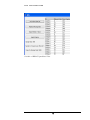
The first two rows of the spreadsheet make up the RDSAT header: The first line must
be RDS. The second line is the sample size, the number of coupons given to each
respondent, the symbol for missing values. In this sample dataset, the number of
respondents in 264, the number of coupons distributed to each respondent is 4, and 0
entries are treated as missing data.
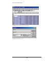
FIGURE 1.2 Sample RDS Data in an Excel Spreadsheet.
* Note: In this sample data set, each recruiter is given 4 coupons to distribute and
the coupon numbers are 8 digits.
3
R D S
I N C O R P O R A T E D
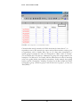
FIGURE 1.3 Excel Spreadsheet – Custom Field Headers and Data..
Column headers must be entered for all fields other than the “main data set” (i.e.
respondent or survey ID, network size, coupon received from recruiter, coupons given
to respondents), such as Gender, Race, Age, etc. If a data value corresponds to a
specific group, for example if a value of 1 corresponds to “Male,” and 2 to “Female,”
you can indicate this in the data set. Abbreviate the group with a single character, for
example ‘m’ for Male and ‘f’ for Female. Add the abbreviations in order of increasing
value to the gender header, surrounded by parentheses. In this example, the resulting
header would be “Gender(mf).” Similarly, to indicate for the Race header that Whites
correspond to group 1, Blacks to group 2 and all other races to group 3, you may use
“Race(WBO).”
4
R D S
I N C O R P O R A T E D
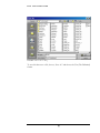
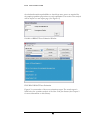
FIGURE 1.4 Excel “Save As” Dialog..
To save this data set to a file, choose, “Save As” and choose the Text (Tab Delimited)
format.
5
R D S
I N C O R P O R A T E D
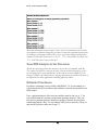
Preparing Data from SPSS
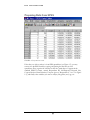
FIGURE 1.5 Sample RDS Data in SPSS.
If the data you wish to analyze is in an SPSS spreadsheet (see Figure 1.5), you may
convert it to the RDS format by copying and pasting the data into an excel
spreadsheet. First, organize the columns so that the “main data set” appears in the
standard RDSAT format, namely Respondent ID, Self-Reported Network Size,
Coupon Received from Recruiter, Coupons given to Respondent (C1 to C3 in Figure
1.5), and finally other variables you want to analyze, like gender, race, age, etc.
6
R D S
I N C O R P O R A T E D
Note: In this sample data set, the variable label for Respondent or Survey ID is “rid”,
for the network size is “net”, for the coupon received from the recruiter is “coupon”
for the coupons given to respondents is “C1-C4.” These variable labels may look
different when exported from RDSCM 3.0 or from the questionnaire data file :
Variable
Variable Label
Data Source
Survey ID
“Survey ID”
RDSCM 3.0
Network Size
“Degree”
Questionnaire data file
Coupon received from recruiter
“Coupon_submitted”
RDSCM 3.0
Coupons given to respondent
“Coupon_given_0”
“Coupon_given_1”
“Coupon_given_2”
RDSCM 3.0
7
R D S
I N C O R P O R A T E D
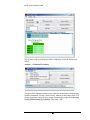
FIGURE 1.6 RDS Data highlighted in SPSS
Highlight all relevant columns in the dataset. To do this, first click on the left-most
column header, this should highlight the entire first column. Next, hold down the
“Shift” key and press the right arrow key until all the desired fields have been
highlighted (see Figure 1.6). Finally either press (Ctrl-C) on the keyboard, or click Edit > Copy on the menu screen to copy the data to the clipboard. Paste this data into the
third line of a blank excel spreadsheet (see Figure 1.7) and add the relevant header
information described in the previous section entitled “Preparing Data from Excel.”
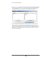
Note
If there are missing data entries in the SPSS dataset, they will be denoted
by a period (‘.’). However RDSAT only accepts integers in the dataset.
Before saving to the Tab Delimited Text Format, you must replace all
occurrences of a period to the missing data value integer. This can be
done by pasting the data into Excel (Figure 1.7) and clicking Edit ->
Replace in the Excel menu bar. In the window that appears, type a period
in the “Find what:” textbox, and the missing data value in the “Replace
with:” textbox (see Figure 1.8). Then click “Replace All.”
8
R D S
I N C O R P O R A T E D
FIGURE 1.7 RDS Data pasted to the third line of an excel spreadsheet
FIGURE 1.8 Excel replace dialog window.
9
R D S
I N C O R P O R A T E D
Preparing data from SAS
If the data to be analyzed is in a SAS data file, then the following steps will transform
the data from a SAS data file to a data file that can be read by RDSAT. First, export
the SAS data file using the following code fragment. The portions highlighted in blue
are specific to the dataset, and must be altered.
data <one>;
set <name of your main SAS data file>;
file <'Target Directory/RDSATdata.txt'>;
put
#1 SurveyID Degree Coupon_submitted Coupon_given_0
Coupon_given_1 Coupon_given_2 age sex race;
Run;
There are two features of note in the above code. First, the output file must be a text
file (suffix .txt) or a data file (suffix .dat). RDSAT only reads these file types. Second,
the variables that comprise the “main data set”: SurveyID Degree
Coupon_submitted Coupon_given_0 Coupon_given_1
Coupon_given_2 must be in the order shown above. Then add variables you
want to analyze, such as age, sex, race. RDSAT requires that the data be placed in this
order and doing so in the output step will save time.
Once the data has been exported, open the file using NOTEPAD (or WORDPAD)
and add the two line header as described in the Section of this chapter entitled
“Preparing Data From Excel.” An example header is displayed highlighted in bold in
the data file fragment below.
The data file is ready to be read by RDSAT. Note that SAS will export the data as a
‘space-delimited’ data file and not a ‘tab-delimited’ data file. RDSAT is capable of
reading both file types. The completed data file will resemble the example below.
RDS
530 11 0 sex agecat race
3 33 1 0 0 0 0 0 0 0 0 0
4 25 2 0 0 0 0 0 0 0 0 0
5 50 3 17 608 607 609 18
6 10 4 20 21 414 416 415
7 40 17 25 23 24 0 0 0 0
0 0
0 0
0 0
622
0 0
10
2
2
0
0
0
2
2
0
0
0
2
2
0 0 1 2 2
0 0 0 1 2 1
1 2 2
R D S
I N C O R P O R A T E D
Preparing Data from the RDS Coupon Manager
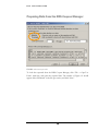
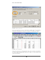
FIGURE 1.9 Excel text import window.
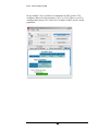
To load data exported from the RDS Coupon Manager, click “File -> Open” in
Excel’s menu bar, and select the exported data. The window of Figure 1.9 should
appear. Select “Delimited” in the file type section, and click “Next.”
11
R D S
I N C O R P O R A T E D
FIGURE 1.10 Excel text import window.
In the next wizard screen, be sure to check the box entitled “Space.” You should see
the data line itself up properly at this point. (see Figure 1.10). Finally, click “Finish.”
FIGURE 1.11 Imported RDSCM Data
Change the network sizes to their appropriate values, and save the data as described in
the section entitled “Preparing Data from Excel.” Figure 1.11 shows fictitious data
exported from RDSCM.
12
R D S
I N C O R P O R A T E D
2
Chapter
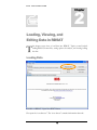
Loading, Viewing, and
Editing Data in RDSAT
T
his chapter covers how to load data into RDSAT. Topics covered include
loading RDSAT format files, setting options for analysis, and viewing/editing
the data.
Loading Data
FIGURE 2.1 RDSAT “Open New RDS” Button
First open the “core data set.” The “core data set” contains information about the
13
R D S
I N C O R P O R A T E D
sample size, missing data values, and number of coupons per respondent.. Start the
RDS Analysis Tool and choose "Open New RDS", or select the file menu and click on
"New RDS" (see Figure 2.1). When a file chooser dialog window appears, select the
RDS data file and choose Open. The nyjazz.txt file included in this distribution is a
good sample file to work with if no real dataset is available. If the default installation
directory was used, this sample file will be located at
C:\Program Files\rdsat\nyjazz.txt
For more information on the “core data set” refer to Appendix? 1. Data pertaining to
other population features of interest can also be included in this file. Analysis cannot be
carried out until this data is loaded.
Note
The sample RDS data set of New York jazz musicians was collected by
Douglas Heckathorn and analyzed in:
"Finding the Beat: Using Respondent-Driven Sampling to Study Jazz
Musicians." Douglas D. Heckathorn and Joan Jeffri. Poetics. (2000)
14
R D S
I N C O R P O R A T E D
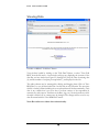
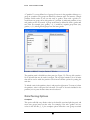
Viewing Data
FIGURE 2.2 RDSAT “Edit Data” Button
View the data loaded by clicking on the "Edit Data" Button, or select "View/Edit
RDS" from the file menu. A new window will pop-up, displaying the contents of the
data files you have loaded (see Figure 2.3). Sample size (264), the value for missing data
(0), and the number of coupons per respondent (7) are displayed on the left.
The table columns may be rearranged by clicking and dragging them. Click on "Save
RDS Data" to save the data loaded into one file with an .rds extension. The next time
this file is loaded, all data including the core and trait data will load automatically. (Trait
data is any variable that is not core data. Core data consists of the respondent id,
network size, and coupons. Trait data can be Race, Age, etc.) Notice that when a cell in
the table is clicked on, its contents may be changed. The changes will be saved to any
data file created with the "Save RDS Data" button.
Note: Be careful not to delete data unintentionally.
15
R D S
I N C O R P O R A T E D
FIGURE 2.3 RDSAT Spreadsheet View
16
R D S
I N C O R P O R A T E D
Setting Options For Analysis
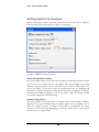
Before conducting an analysis, check the options that will be used. Choose "Options"
from the main window. The window of figure 2.4 will appear
FIGURE 2.4 RDSAT Options Window
Adjust Average Network Sizes
In a chain referral sample, those with more connections and larger personal network
sizes tend to be over-represented in the sample. This can potentially bias sample
estimates. The phenomenon can be corrected, however, and the RDS analysis tool
does so by default. To learn more about the methods used refer to: "Sampling and
Estimation in Hidden Populations Using Respondent-Driven Sampling" by Douglas
Heckathorn and Mathew Salganik. If you do not wish to adjust the average network
sizes for this sample bias, uncheck the flag.
Number of Re-samples
This is the number of times the data is re sampled to derive the bootstrap confidence
intervals. For accurate confidence intervals, keep this option at least the default value of
2500. For optimal accuracy, a number over 15,000 is recommended. Be aware,
however, that the bootstrap is demanding of CPU time. There may be a short wait if
this value is set to a high number.
17
R D S
I N C O R P O R A T E D
Confidence Interval
The value of this parameter determines the level of confidence for the confidence
intervals reported in the analysis. The default, .05, measures the normalized length of a
tail of the distribution of population proportions. In short, it determines 90%
confidence for the intervals reported in the analysis.
Pull-In Outliers of Network Sizes
With this option you may eliminate extremely small and large outliers in network sizes.
Check the box, and input the desired percentages of each end of the network
distribution you would like to be pulled-in (For example, a value of 5% would pull-in
the top 5% and bottom 5% of the network size values). If this option is selected, when
the program encounters an individual whose network size is outside of the specified
bounds, their network size will be set to the value of the nearest lower or upper bound
(percentage). A modest value is recommended. To view the changes, use the
"View/Edit" utility. The changes enacted by the "Pull-In Outliers of Network Sizes"
option may then be saved to a data file.
Note: Check for outliiers by running a univariate frequency in SAS/SPSS/Excel
before importing data to RDSAT.
Algorithm Type
Three different algorithms are available for analyzing an RDSAT dataset: Linear Least
Squares (LLS), Data Smoothing, and Enhanced Data Smoothing. The recommended
algorithm is “Data Smoothing,” which adjusts recruitments across groups, providing
tighter Confidence Intervals than the naïve LLS method. Enhanced Data Smoothing
assigns tiny, non-zero number to all cells in recruitment matrix, then uses Data
Smoothing. This allows for an analysis to include non-recruiting groups, which would
normally fail using LLS or Data Smoothing.
18
R D S
I N C O R P O R A T E D
3
Chapter
Analyzing a Dataset
T
his chapter introduces the analysis features of RDSAT. This is the heart of the
software’s functionality. Topics include Partition Analysis, Breakpoint
Analysis, and Custom Analysis.
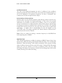
Partition Analysis
If an RDS dataset is successfully loaded, click on "Analyze Partition" in the
upper right of the main window. (see Figure 3.1). By clicking on this button,
the window of Figure 3.2 will appear.
FIGURE 3.1 RDSAT “Analyze Partition” Button
19
R D S
I N C O R P O R A T E D
A "partition" is a user-defined set of groups. Everyone in the population belongs to a
group in a partition. The groups are defined by common traits. For instance, a simple
partition would consist of just one trait such as, gender. Those with a gender of 1
would form one group, those with gender of 2, another. A multi-trait partition of race
and gender can also be created. A group would then be defined by both a gender and
race value. For example, (race, gender) = (1, 1) would be a separate group from (race,
gender) = (2, 1) although both groups have the same gender.
FIGURE 3.2 RDSAT “Analyze Partition” Window
The partition panel is divided into three parts (see Figure 3.2). The top left contains a
list of all traits that may be used for analysis. The top right contains a list of all traits
that will be used to make the partition. The bottom contains options for parsing the
trait data.
To include a trait in the partition, select it and press the right-arrow. To remove it from
the partition, select it and press the left-arrow. For each of the traits included in the
partition, how to parse the data values must be selected.
Data Parsing Options
Complete
This option will find every distinct value in the data file associated with that trait, and
create new groups based on that value. For example, if the trait "gender" has two
values in the data file, (1, 2), the complete option will make a new group associated
20
R D S
I N C O R P O R A T E D
with each of these values. If the trait "race" has three values (10, 11, 12), then the
complete option will create 3 more groups corresponding to those trait values. If both
gender and race are included in the partition, there will be 2 x 3 = 6 groups in all:
(race, gender) = {(10, 1), (11, 1), (12,1), (10, 2), (11, 2), (12, 2)}
Breakpoint
This will take every value below the specified breakpoint and create a new group based
on it; a 2nd group is created based on every value greater than or equal to the specified
breakpoint. This is different from a “breakpoint analysis” (discussed in the next
section) in that only one breakpoint is chosen for the dataset, rather than a range of
breakpoints. The analysis is identical to a complete partition analysis with the exception
of creating exactly 2 groups from a partition in the dataset, rather than one for every
possible trait value.
For example, the trait "age" has a range of values associated with it. It would be
impractical to create a group for every distinct age, but by choosing breakpoint with a
value of 40, the population can be divided into a group less than 40 years old and a
group greater than 40 years old.
Analyze Continuous Variable
This feature parses the data so that each cell in the recruitment matrix is as close as
possible to the number entered in the field. The default is 30 because most statistical
procedures require each cell in the matrix have 30 or more cases. The results are
interpreted in the same way as a partition analysis.
Custom
This allows partitions to be created based on non-overlapping ranges of values. For
instance, selecting a trait such as age and using a custom partition with parameters. {10,
20}, {21, 30}, {31, 40}, {41, 50} would create 5 groups based on 5 intervals of ages.
Each range must be enclosed in curly-braces and delimited with commas. Ranges
should not overlap. Upper and lower bounds may be the same however (e.g. {30, 30})
if a group must be based on only one value.
Note
It is very easy to create a partition with a great number of groups, such as
by selecting complete with a trait with many values (e.g. age). In general,
the amount of data is insufficient to handle partitions with such a large
number of groups and the analysis will fail.
21
R D S
I N C O R P O R A T E D
Breakpoint Analysis
Breakpoint analysis allows one trait to be analyzed over a range of possible breakpoints.
This is very useful for continuous variables, such as age.
FIGURE 3.3 RDSAT “Analyze Breakpoint” Button
To analyze a breakpoint, click on "Analyze Breakpoint" in the main window (see
Figure 3.3). A Breakpoint analysis can be done on any trait, but it is more effective to
use traits with many variables, such as 'age' in the data set of New York jazz musicians.
The bound fields allow the range of variables to be chosen over which the breakpoint
will be set.
For example, from the NYC Jazz dataset (located in the RDSCM distribution folder,
see Chapter 2 for details), 'age' is selected from the drop down list. The step size is set
to 1, and 25 and 50 are entered for the lower and upper bound (see Figure 3.4). This
will perform a breakpoint analysis for groups above and below 25, then above and
below 26, and so on.
22
R D S
I N C O R P O R A T E D
FIGURE 3.4 RDSAT Breakpoint Analysis Window
In the above window, we are selecting “Age” as the variable to be analyzed, and
choosing where the breakpoints will lie. A “Step” of 5 with lower and upper
bounds of 25 and 50 will break the dataset into the following (7) categories:
• Recruits age 25 or under
• Recruits 26-30
• Recruits 31-35
• Recruits 36-40
• Recruits 41-45
• Recruits 46-50
• Recruits age 51 or older
Likewise a Step of 1 would produce 27 different categories, one for recruits 25 or
under, one for a recruit of every age between 25 and 50, and one for recruits age
51 or
older.
23
R D S
I N C O R P O R A T E D
4
Chapter
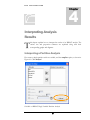
Interpreting Analysis
Results
T
his chapter explains how to interpret the results of an RDSAT analysis. The
various size and proportion estimates are explained along with their
corresponding graphs and diagrams.
Interpreting a Partition Analysis
First create a simple partition with one variable, and the complete option, as shown in
Figure 4.1. Click Analyze!
FIGURE 4.1 RDSAT Single Variable Partition Analysis
24
R D S
I N C O R P O R A T E D
After a moment, the results of the analysis will be output to the pages in the main
window. To move between pages of the analysis, click on its corresponding tab.
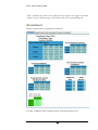
Recruitment
Displays general statistics regarding the recruitment.
FIGURE 4.2 RDSAT Single Variable Partition Analysis Recruitment Tab
25
R D S
I N C O R P O R A T E D
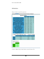
Key of Group and Trait Correspondence
The green “Key of Group and Trait Correspondence” (at the bottom) is used to
interpret the data related to recruitment in the analysis. It lists all of the various groups
that were analyzed, and relates them to the trait they have in common. In this example,
Group 0 corresponds to Race #1. Looking at the Race variable, we see that the races
are listed in parentheses by their initials, WBO (W – White, B – Black, O – Other). So
Group 0 corresponds to the first race in the list, “White.” Group 1 corresponds to
“Black,” and Group 2 to Other.
Recruitments
Matrix of recruitments to and from each group. The vertical axis (rows) depicts the
recruiters and the horizontal axis (columns) show recruits. For example, this matrix
tells us that Group 0 recruited 36 other people in Group 0.
Transition probabilities
Normalizes recruitments by dividing by the total number of recruitments and gives the
probability of one group recruiting another. For example Group 1 recruited 94 from
the same group, and so the normalized transition probability is 94 / (94 + 32 + 18) =
.652, where the denominator is the total number of recruits Group 1 made.
Demographically-adjusted Recruitment Matrix
Gives hypothetical recruitments if each group recruited with equal effectiveness.
Transition probabilities implied by this matrix are identical to those of the original
Recruitment Matrix.
It is well known that some groups of respondents recruit more than others, e.g., HIV
positives often recruit substantially more than do negatives. This is shown in the
recruitment matrix if the number of recruitments by HIV positives (i.e., the row sum in
the matrix) exceeds the number of recruitments of HIV positives (i.e., the column sum
in the matrix). The demographically adjusted recruitment matrix shows what the
recruitment matrix would have looked like if all groups had recruited equally (i.e., so
row and column sums are equal), without any change in recruitment patterns (i.e., no
change in transition probabilities).
This type of adjusted matrix is useful for testing one of the assumptions of the
statistical theory on which RDS is based, which holds that if recruitment effectiveness
is uniform across groups, cross group recruitments will tend to be equal. Therefore, the
cross-group recruitments in the adjusted matrix will differ only by amounts consistent
with stochastic variation.
26
R D S
I N C O R P O R A T E D
Thus, if positives recruit more than negatives then in the original recruitment matrix, all
else equal, the number of negatives recruited by positives will tend to be greater than
the number of positives recruited by negatives. However, in the demographically
adjusted matrix these will be, if not equal, at least strongly correlated.
Sample population sizes
Reports the total number of recruits in each group.
Initial Recruits
Reports the number of "seeds" from each group, i.e. people recruited by the
researcher in each group.
Note
Much of the data reported above also have corresponding data-smoothed
estimates. Data-Smoothing is a method for eliminating deviations in
cross-group recruitments that occur due to chance. For more
information about data-smoothing, refer to Douglas D. Heckathorn:
2002, "Respondent Driven Sampling II: Deriving Valid Population
Estimates from Chain-Referral Samples of Hidden Populations." Social
Problems v.49, No. 1, pages 11-34.
27
R D S
I N C O R P O R A T E D
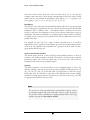
Estimation
Displays estimates of population proportions.
FIGURE 4.3 RDSAT Single Variable Partition Analysis Estimation Tab
28
R D S
I N C O R P O R A T E D
Total Distribution of Recruits
The raw count of recruits in the data set for each group. The “total” is the sample size
minus the number of seeds.
Estimated Population Proportions
The estimated population proportion can either be calculated using the linear least
squares algorithm, or the data-smoothing algorithm, depending on how the
options are set for the RDS analysis. In the above diagram, the data smoothing
algorithm was used. See the “Algorithms” section of Chapter 2 for more
information on the difference between various estimation algorithms in RDSAT.
1) Least-Squares Population Proportions
Reports the estimated population proportions of each group using linear least
squares to solve the population equations.
2) Data-Smoothed Population Proportions
Reports estimated population proportions for the Data-Smoothed population
equations.
Sample Population Proportions
Report the sample population proportions, also called the "naive" estimates of
population proportions. The term naïve is used because the proportion is a simple
ratio of how many of a particular group were recruited to the total number of
recruits. It is not adjusted for any statistical biases. (To learn more about the
methods used refer to: "Sampling and Estimation in Hidden Populations Using
Respondent-Driven Sampling" by Douglas Heckathorn and Mathew Salganik).
Recruitment Proportions
The unadjusted recruitment proportions for the sample. This is the same as the
“Sample Population Proportions” if seeds were not included in the calculation.
Equilibrium Sample Distribution
The equilibrium sample population proportions indicate each group’s population
size after the proportions have converged to their equilibrium value. This occurs
when further recruitment waves do not change the population proportion by a
significant amount.
Mean Network Size, N (adjusted)
Network sizes are adjusted for sampling bias. In a chain referral sample, those
with more connections and larger personal network sizes tend to be overrepresented in the sample. This can potentially bias sample estimates. (To learn
more about the methods used refer to: "Sampling and Estimation in Hidden
Populations Using Respondent-Driven Sampling" by Douglas Heckathorn and
Mathew Salganik).
29
R D S
I N C O R P O R A T E D
Mean Network Size, N (unadjusted)
Straight-forward arithmetic mean of the sample’s network sizes.
Homophily (Hx)
A measure of preference for connections to one's own group. Varies between -1
(completely heterophilous) and +1 (completely homophilous).
Affiliation Homophily (Ha)
A homophily measure based on the equilibrium proportions. It provides a measure of
homophily which is not effected by differential degree across groups.
Degree Homophily (Hd)
A measure of the level of homophily that is attributable to differential degree across
groups.
Population Weights:
The population weights can either be calculated using the linear least squares
algorithm, or the data-smoothing algorithm, depending on how the options are set
for the RDS analysis. In the above diagram, the data smoothing algorithm was
used. See the “Algorithms” section of Chapter 2 for more information on the
difference between various estimation algorithms in RDSAT.
1) LLS Population Weights
Multiplicative factors by which the Least Squares Estimates are different from the
naive estimates.
2) Data-Smoothed Population Weights
Multiplicative factors by which the Data-Smoothed Estimates are different from
the naive estimates.
Recruitment Component (RCx)
The recruitment component of the RDS estimator:
(RCx) * (DCx) = RDS estimator for group x
Degree Component (DCx)
The degree component of the RDS estimator.
(RCx) * (DCx) = RDS estimator for group x
Standard Error of P
The standard error of the RDS estimator, based on the RDS bootstrapping algorithm.
Confidence Intervals
Are obtained by bootstrapping the original sample. The confidence intervals only
correspond to the Least Squares population estimates and can be set in the
options panel (click "options" in the main window).
30
R D S
I N C O R P O R A T E D
Network Sizes and Homophily
This tab displays Homophily, Affiliation, and Average Network Sizes.
FIGURE 4.4 RDSAT Single Variable Partition Analysis Network Sizes Tab
Adjusted Average Network Sizes
Network sizes are adjusted for sampling bias. In a chain referral sample, those
with more connections and larger personal network sizes tend to be overrepresented in the sample. This can potentially bias sample estimates. (To learn
more about the methods used refer to: "Sampling and Estimation in Hidden
Populations Using Respondent-Driven Sampling" by Douglas Heckathorn and
Mathew Salganik).
Unadjusted Network Sizes
Straight-forward arithmetic mean of the sample’s network sizes.
31
R D S
I N C O R P O R A T E D
Network Size Information
Displays the minimum and maximum network sizes for the sample.
Homophily
A measure of preference for connections to one's own group. Varies between -1
(completely heterophilous) and +1 (completely homophilous).
Affiliation Matrix
Displays the same preference measures, but for all group pairs.
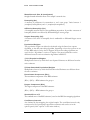
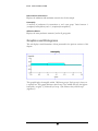
Graphics and Histograms
This tab displays visual illustrations of data presented in the previous sections of this
chapter.
This graph displays homophily within 3 different groups. Each group is shown as
a separate bar. This graph illustrates that Group 2 (the middle bar) has the highest
homophily (roughly .3), followed by Group 1 (the leftmost bar) and Group 3
(rightmost).
32
R D S
I N C O R P O R A T E D
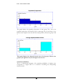
This graph displays the population proportions of each group. The y axis is the
population proportion, and should be read as a percentage. We see that Group 1, (the
leftmost bar) comprises more than half the total population, followed by group 2 and
3.
This graph displays the adjusted network sizes of each group. Observe that
group 3, (the rightmost bar) has the highest network size.
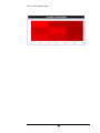
Transition Probabilities
This is a 2 dimensional histogram of the transition probabilities. A brighter color
corresponds to a higher value. It is a method of visualizing the corresponding
transition matrix.
33
R D S
I N C O R P O R A T E D
34
R D S
I N C O R P O R A T E D
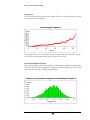
Degree List
List of all network sizes reported in the sample. The list is sorted from least to greatest
for easy view of the distribution.
In the graph above we see that there are a few respondents with networks as large
as 900, but most respondents fall within a degree of 100-300.
Bootstrap Simulation Results
Shows the histogram of Bootstrap estimates of Least Squares population proportions.
The horizontal axis depicts population estimates for the specified group. The vertical
axis shows the frequency of the Bootstrap estimate.
35
R D S
I N C O R P O R A T E D
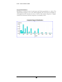
Degree Distributions
Distribution of network sizes for each group and for the population as a whole. The
diagram below happens to be of the entire population. We see that most members of
the population have network sizes close to 100 or 200, and the frequency of higher
network sizes decreases with the exception of an anomaly at 500.
36
R D S
I N C O R P O R A T E D
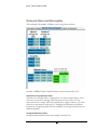
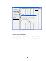
Interpreting a Breakpoint Analysis
A breakpoint analysis breaks a dataset into groups based on a single continuous
variable. A continuous variable of interest might be “Age,” where one wouldn’t
examine each individual age as a separate group, but rather a range of Ages. As
such there is no recruitment data for breakpoint analyses. Rather there are
interesting trends to notice in Homophily and population proportion as the
breakpoint is shifted and respondents are moved from the upper group of the
lower group. The Estimation tab shows a table of Least Squares population
estimates corresponding to each breakpoint value. Similarly, the Network Sizes
and Homophily tables are arranged by breakpoint value (see Figure 4.5).
FIGURE 4.5 RDSAT Breakpoint Analysis Estimation Tab
37
R D S
I N C O R P O R A T E D
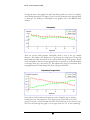
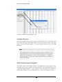
Viewing the data in the graphics tab will often make patterns very clear. For example,
in the breakpoint analysis of Chapter 3, New York Jazz musicians were analyzed based
on their age. Try clicking on Homophily in the graphics tab of the RDSAT main
window…
There are several visible patterns: Homophily tends to zero as the age variable
increases. This implies that differences in age become less important for choosing
relationships the older the recruits are. It is also notable that the older group is always
more homophilous than the younger group. Finally, it is possible to see that homophily
is strongest where age is the lowest (25). This implies that young jazz musicians show
strong preference for relationships with other young jazz musicians.
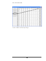
Next click on LLS Population Proportions on the Graphics page to find the
breakpoint where the population of the upper group equals that of the lower
group. From this it can be inferred that half of the musicians are less than 43 years
old. Note that although the graph’s x-axis ranges from 0 to 25, we are conducting
38
R D S
I N C O R P O R A T E D
a breakpoint analysis on groups age 25 to 50. Therefore the above intersection
corresponds to an age of 43 (18+25), not 18.
39
R D S
I N C O R P O R A T E D
5
Chapter
Handling Missing Data in
the Dataset
M
ost data sets contain missing data. RDSAT offers two ways of setting
missing data. Both of these options will be covered in this chapter.
RDSAT employs two features to handle missing data. The first makes it
possible to reassign another value to missing data. In this way, respondents for
whom data is missing can be included in the analysis, to see if missing data is
random or associated with other variables. For example, in an analysis of HIV
prevalence, respondents would be divided into three categories, positive, negative,
or missing. One could then run analyses (in a statistics program) to see if having
missing data was correlated with other terms such as race/ethnicity. The other
data imputation procedure sets missing values at the median of the variable.
Replace Missing Data
This feature is found in the “Edit Data” menu. It allows each trait to be chosen and to
specify which value the missing data within that trait should have. This option can also
be used to give missing data a unique value to allow groups to form on the basis of
whether they have missing data. For reference, the missing data value is displayed on
the left-hand side of the Edit Data screen. To use this feature, click “Replace Missing
Data.” In the pop-up, select both the trait for which data is to be replaced and the
value to which it should be set. Click “Commit Changes” to replace data. Then click
“Save RDS Data File” to make changes permanent. To re-analyze a dataset, close the
Edit Data screen and run new analyses.
40
R D S
I N C O R P O R A T E D
FIGURE 5.1 RDSAT Replace Missing Data
Impute Median Values
This feature calculates the median value of the trait being analyzed and replaces all
missing data cells with this median value. First, click “Impute Median Values” on the
left side of the Edit Data screen. Select the trait you want to replace values in and click
“Commit Changes.” To make the changes permanent, click “Save RDS Data File.”
41
R D S
I N C O R P O R A T E D
FIGURE 5.2 RDSAT Impute Median Values
Impute Degree
This feature imputes missing values on degree (Network Size). To use this feature, first
run a partition analysis. This analysis defines the groups that will be used to impute the
degree. Next, click “Impute Degree.” To make changes permanent, click “Save RDS
Data File.”
Note
The “Impute Degree” feature only functions after a partition has been
analyzed because it uses the mean unadjusted network size for the group
(defined by the partition) in which each respondent is a member to
impute the degree. To learn more about partition analysis, see Chapters 3
and 4 of this manual.
Add Field Sample Weights
This feature adds the Field Sample Weights to the RDS data file. It only appears in the
Edit Data screen when a partition has been analyzed. In the Edit Data screen, click
“Add Field Sample Weights.” A new column of data will appear that contains the
Field Sample Weights. Click “Save RDS Data File” to make this change permanent.
42
R D S
I N C O R P O R A T E D
FIGURE 5.3 RDSAT Add Field Sample Weights
43
R D S
I N C O R P O R A T E D
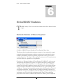
6
Chapter
Extra RDSAT Features
T
he RDS Analysis Tool has several extra features that will be discussed in this
chapter.
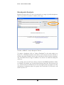
Estimate Number of Waves Required
FIGURE 6.1 RDSAT Estimate Number of Waves Required Menu Item
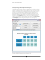
This feature allows hypothetical recruitment scenarios to be examined. A group is
selected to be the initial recruiters, and they are allowed to recruit based on their
transition probabilities, until the population proportions converge to the actual
sample proportions. This helps in determining how many waves of recruitment are
necessary before the population is at equilibrium.
First click on “Estimate Number of Waves Required” in RDSAT’s Analyze menu.
This will cause the window of Figure 6.2 to appear. Then select a starting group
for a hypothetical sample. Next, choose a convergence radius. The smaller this
number, the higher the confidence intervals will be. However, the dataset will take
longer to analyze. The default is .02, which should serve as a good starting point.
A radius of .02 means that the population proportions will change by less than .02
with further recruitment. In other words, the sample population proportions are
considered converged (at equilibrium) when the change in population proportions
in between waves is less than the convergence radius times of the population
proportions. Select analyze, and this utility will use the Markov process implicit in
44
R D S
I N C O R P O R A T E D
the calculated transition probabilities to check how many waves are required for
the sample population proportions to reach equilibrium. The results of the analysis
will be output to a new report page. (See Figure 6.3)
FIGURE 6.2 RDSAT Waves Estimation Window
FIGURE 6.3 RDSAT Waves Estimation
Figure 6.3 is ascreenshot of the waves estimation output. The actual output is
listed below for a partition analysis of the New York Jazz dataset (See Chapter 2
for more information on this dataset).
45
R D S
I N C O R P O R A T E D
What this information means is that it took a total of 4 recruitment waves before
the population estimates changed by less than .02 times the population proportion
(Assuming a convergence radius of .02). As we can see the change in proportion
estimates of Group 1 from wave 3 to 4 is .79 - .778 = .012, which is less than .02 *
.79 = .0158. The same is true of Group 2.
Save RDS Analysis in the File menu
Allows the report pages from the analysis to be saved to a formatted .html file.
The analysis can then be viewed at any time with any web browser and it can be
cut and pasted onto most spreadsheets. In the current version of RDSAT, only
saving to HTML is possible, however copying and pasting should allow the data to
be imported into many applications including plain text editors.
Estimate Prevalence
Prevalence estimation is now possible with RDSAT 5.6. As an example, we
will determine the HIV prevalence and confidence interval among males in an
RDS sample.
First, a partition analysis of the relevant variables must be run (see p. 17 for
more information on executing a multivariate partition analysis). Once you
have done a partition analysis, identify the groups of interest for prevalence
estimation using the “Key”. In our example, HIV positive males are Group 1.1
and non-HIV positive males are Group 1.2.
46
R D S
I N C O R P O R A T E D
We are now ready to perform prevalence estimation. From the menu items
select:
Analyze –> Estimate Prevalence
The prevalence function requires you to enter the denominator and numerator
used for estimation. Use the “Select Group” buttons to enter these fields. The
groups appearing in the pull down menu correspond to groups from the most
recent partition analysis preformed. Then click “OK”.
47
R D S
I N C O R P O R A T E D
In our case, we want the prevalence of HIV among males within the population.
Thus, the numerator is Group 1.1 (HIV positive males) and the denominator
contains BOTH Group 1.1 and Group 1.2 (non-HIV positive males).
Once the analysis is performed, the output will appear in a new tab called
“ratio”. The output contains a prevalence estimate and confidence interval for
that estimate as well as those groups used by the function and Key of Group
and Trait Correspondence.
48
R D S
I N C O R P O R A T E D
In our example, 14.9% of males are estimated to be HIV positive. The
confidence interval for this estimate is 10.3% to 19.6%. Thus we are 95%
confident that between 10.3% and 19.6% of males are HIV positive in this
population.
49
R D S
I N C O R P O R A T E D
7
Chapter
The RDSAT File Menu
T
he RDS Analysis Tool File Menu has multiple features located in it. This
chapter describes how to use them.
RDS Analysis Tool File Menu Features
New RDS
This feature allows one to open a new RDS data set. The button “Open New RDS”
(on the main screen) serves the same function.
View/Edit RDS
This feature opens the Edit Data screen. The “Edit Data” button (on the main screen)
serves the same function.
Save RDS Analysis
This feature saves an RDS partition analysis in the form of a text file. It can be
imported to Excel® as a delimited file.
Print…
This feature prints an RDS analysis.
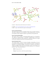
Export DL Network File
Allows a DL network file to be exported to the recruitment chain data. DL format is
recognized by numerous network analysis packages, including UCI-net and Pajek.
Pajek in particular, can be used to create attractive social network visualizations as seen
in Figure 7.1.
50
R D S
I N C O R P O R A T E D
FIGURE 7.1 Pajek Generated Social Network Visualization
UCINET - http://www.analytictech.com//ucinet_5_description.htm
PAJEK - http://vlado.fmf.uni-lj.si/pub/networks/pajek
Export Population Weights
This function exports a text file of Population Weights (From “Population Estimates”
table under “Estimation” tab, See XXXX) for each respondent based on the most
recent partition analysis. Weights are linked to respondents by the respondent ID.
Export Individualized Weights
This function export a text file of individualized RDS weights for each respondent.
The weights are calculated based on respondents’ individual degrees and the latest
partition analysis performed. When generated for a dependent variable, these weights
can be used to weight the entire data set for multivariate analysis.
Export Estimation Table
This function exports a text file of output and weights, corresponding to the most
recent partition analysis preformed, for each respondent in the data. In essence, this
reproduces the “Population Estimates” table from the “Estimation” tab in RDSAT,
therefore a partition analysis MUST be performed in order for this function to be
available (See XXXX in this manual for more detailed explanation of the “Population
Estimates” table). The exported fields are:
RID: The Respondent ID
Group: Group number to which the respondent belongs
51
R D S
I N C O R P O R A T E D
PopEst: The RDS population proportion estimate of the respondent’s group.
Sample: The sample proportion of the respondent’s group.
RecruitProp: The recruitment proportion of the respondent’s group.
Equilibrium: The equilibrium proportion of the respondent’s group.
Hx: The RDS homophily measure for the respondent’s group.
Ha: The affiliation homphily measure for the respondent’s group.
Hd: The degree homphily measure for the respondent’s group.
Weight: The population weight for the respondent’s group.
RecComponent: The recruitment component for the respondent’s group (RCx).
DegComponent: The degree component for the respondent’s group (DCx).
IndDegreeComp: The degree component based on the respondent’s individual
degree. This value is unique to the respondent.
IndweightComp: The individualized RDS estimator weight based on
respondent’s degree and the partition variable. When calculated for a dependent
variable, the data set can be weighted by this value for multivariate analysis.
Degree: The respondent’s degree or personal network size.
Export Table of Recruitments
Options
This feature opens the options menu. The “Change Options” button (on the main
screen) serves the same function.
Exit
This feature exits the RDS Analysis Tool program. It serves the same function as the
“x” in the top right-hand corner of Windows® programs. NOTE: Make sure not to
close the program without saving necessary data changes.
52
R D S
I N C O R P O R A T E D
RDS Glossary of Terms
Adjust Average Network Size Option
In a chain referral sample, those with more connections and larger personal network
sizes tend to be over-represented in the sample. This RDSAT option corrects this bias.
Adjusted Average Network Sizes
Network sizes that are adjusted for sampling bias.
Affiliation Matrix
Displays preference measures for connections between all group pairs. The diagonal of
this matrix is Homophily within a group.
Bootstrap Simulation Results
Shows the histogram of Bootstrap estimates of Least Squares population proportions.
The horizontal axis depicts population estimates for the specified group. The vertical
axis shows the frequency of the Bootstrap estimate.
Breakpoint Analysis
A Breakpoint analysis allows one trait to be analyzed over a range of possible
breakpoints. This is very useful for continuous variables, such as age.
Complete Variable Analysis
This option will find every distinct value in the data file associated with a variable trait,
and create new groups based on that value.
Confidence Interval
The value of this parameter determines the level of confidence for the confidence
intervals reported in the analysis. The default, .05, measures the normalized length of a
tail of the distribution of population proportions. In short, it determines 90%
confidence for the intervals reported in the analysis.
Cut Outliers
An RDSAT option that eliminates extremely small and large outliers in network sizes
from the dataset.
Data-Smoothed Population Proportions
Reports estimated population proportions for the Data-Smoothed population
equations.
Data-Smoothed Population Weights
Multiplicative factors by which the Data-Smoothed Estimates are different from the
naive estimates.
53
R D S
I N C O R P O R A T E D
Degree Distributions
Distribution of network sizes for each group and for the population as a whole.
Degree List
List of all network sizes reported in the sample. The list is sorted from least to greatest
for easy view of the distribution.
Demographically-adjusted Recruitment Matrix
Gives hypothetical recruitments if each group recruited with equal effectiveness.
Transition probabilities implied by this matrix are identical to those of the original
Recruitment Matrix.
DL Network File
DL format is recognized by numerous network analysis packages, including UCI-net
and Pajek. Pajek in particular can be used to create attractive social network
visualizations.
Enhanced Data Smoothing
An RDSAT option that allows analysis to take place even in a dataset with no
recruitment data for a particular group.
Homophily
A measure of preference for connections to one's own group. Varies between -1
(completely heterophilous) and +1 (completely homophilous).
Impute Missing Data and Re-Analyze
Sets missing data to their most probable value, given the transition probabilities.
Initial Recruits
Reports the number of "seeds", i.e. people recruited by the researcher in each group.
Least-Squares Population Proportions
Reports the estimated population proportions of each group using linear least squares
to solve the population equations.
LLS Population Weights
Multiplicative factors by which the Least Squares Estimates are different from the
naive estimates.
Partition
A user-defined set of groups. Everyone in the population belongs to a group in a
partition. The groups are defined by common traits.
Re-Analyze with Specified Missing Data
This feature allows each trait to be chosen and to specify which value the missing data
within that trait to have. It can also be used to give missing data a unique value to allow
groups to form on the basis of whether they have missing data.
54
R D S
I N C O R P O R A T E D
Recruitment Matrix
Matrix of recruitments to and from each group. The vertical axis (rows) depicts the
recruiters and the horizontal axis (columns) show recruits.
Re-samples
This is the number of times random subsets of the data are sampled to derive the
bootstrap confidence intervals. More re-sampling will result in better confidence
intervals, but will be more CPU intensive.
Respondent
A participant in an RDS sampling study.
Respondent ID
A unique integer representing a respondent in a given RDS dataset.
Sample Population Proportions
The "naive" estimates of population proportions, without correction of over-sampling
and other biases.
Sample Population Sizes
The total number of recruits in each group.
Self-Reported Network Size
The number of individuals a respondent reports he or she has in his/her network.
Transition Probabilities
Normalizes recruitments by dividing by the total number of recruitments and gives the
probability of one group recruiting another.
Unadjusted Network Sizes
A straight-forward arithmetic mean of the sample’s network sizes.
Waves Estimation
This feature allows hypothetical recruitment scenarios to be examined. The sample
population proportions are considered converged when the change in population
proportions in between waves is less than the convergence radius times of the
population proportions.
55
R D S
I N C O R P O R A T E D
References
• "Respondent-Driven Sampling: A New Approach to the Study of Hidden Populations." By
Douglas D. Heckathorn. Social Problems 44: 174-199
o The original article in which RDS was introduced
• "Respondent-Driven Sampling II: Deriving Valid Population Estimates from Chain-Referral
Samples of Hidden Populations." By Douglas D. Heckathorn Social Problems, 2002.
o Article extending the RDS method to include calculation of standard errors and
post-stratification to control for differences in network size and clustering across
groups
• Salganik, Matthew J. and Douglas D. Heckathorn. In press (December, 2004) “Sampling and
Estimation in Hidden Populations Using Respondent-Driven Sampling.” Sociological
Methodology.
o Article showing through both analytic means and simulations that the RDS
population estimator is statistically unbiased
o Outstanding Article Publication Award of the Mathematical Sociology Section of
the American Sociological Association
• "Extensions of Respondent-Driven Sampling: A New Approach to the Study of Injection
Drug Users Aged 18-25." By Douglas D. Heckathorn, Salaam Semaan, Robert S.
Broadhead, and James J. Hughes. AIDS and Behavior, 2002.
o Empirical evaluation of some of the assumptions underlying RDS, and its use to study
younger drug injectors
• "Group Solidarity as the Product of Collective Action: Creation of Solidarity in a Population
of Injection Drug Users." By Douglas D. Heckathorn and Judith E. Rosenstein. Advances
in Group Processes, 2002.
• "Development of a Theory of Collective Action: From the Emergence of Norms to AIDS
Prevention and the Analysis of Social Structure." By Douglas D. Heckathorn In New
Directions in Sociological Theory: Growth of Contemporary Theories (Joseph Berger and
Morris Zelditch, editors). Rowman and Littlefield, 2002.
o History of RDS and the research project from which it emerged
• Heckathorn, Douglas D., and Joan Jeffri. 2003. “Social Networks of Jazz Musicians,” pp. 4861 in Changing the Beat: A Study of the Worklife of Jazz Musicians, Volume III:
Respondent-Driven Sampling: Survey Results by the Research Center for Arts and Culture,
National Endowment for the Arts Research Division Report #43, Washington DC, 2003.
o Use of RDS to study a non-stigmatized hidden population, jazz musicians
• “Finding the Beat: Using Respondent-Driven Sampling to Study Jazz Musicians.” By
Douglas D. Heckathorn and Joan Jeffri. Poetics, 2001.
o Use of RDS to study a non-stigmatized hidden population, jazz musicians
56
R D S
I N C O R P O R A T E D
• “Making Unbiased Estimates from Hidden Populations Using Respondent-Driven
Sampling.” By Matthew J. Salganik and Douglas D. Heckathorn. Paper presented at the
International Social Network Conference, February, 2003, Cancun, Mexico
• “ Street and Network Sampling in Evaluation Studies of HIV Risk-Reduction
Interventions.” By Salaam Semaan, Jennifer Lauby, and Jon Liebman. AIDS Review, 2002.
o Comparison and Evaluation of Alternate Methods for Sampling Hidden Populations.
• "Review of Sampling Hard-to-Reach and Hidden Populations for HIV Surveillance." By
Robert Magnani, Keith Sabin, Tobi Saidel, and Douglas Heckathorn. In AIDS, 2005.
57
R D S
I N C O R P O R A T E D
Appendix
I
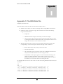
Appendix 1: The RDS Data File
Components of Core Data Files:
Note that all data outside of the first two lines must be integer-valued.
•
Header on line 1: Every core data set must begin with the string 'RDS' on the first line.
•
Parameters on line 2: From left to right, the second line must contain the following
integer-valued information:
•
o
Sample Size
o
Maximum number of coupons received by a recruit in the sample
o
Value for missing data. This value will be used throughout the analysis to refer
to missing data. It will over-ride all other values, so it is important to choose an
integer value that will not occur elsewhere in the data.
Main data: Subsequent lines contain the main recruitment information with each line
corresponding to a recruit. Arrange the columns from right to left as followed:
o
Recruit ID: an integer code, acting as the recruit's name
o
Personal Network Size
o
The serial number of the coupon the recruit recieved. NOTE: if the recruit is a
'seed', then this number must be set to the missing-data value.
o
Serial numbers of the coupons given to the recruit. This data will take up the
number of columns specified by the max-number-of-coupons-given-to-a-recruit
parameter specified on line two. If the recruit was given a number of coupons
less than that, set some of the values to the missing-data value.
For example, below are the first 7 lines of the core data set for Doug Heckathorn's New York jazz
musicians:
RDS
264 7
1 350
2 0 0
3 585
4 400
5 150
0
0 14250004 14250005 14250006 14256002 901
14250007 14250008 14250009 14256003 902 0
0 14250010 14250011 14250012 14256004 903
0 14250025 14250026 14250027 14256009 904
0 14250022 14250023 14250023 14256008 905
58
0
0
0
0
0
0
0
0
0
R D S
I N C O R P O R A T E D
Appendix
II
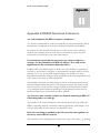
Appendix 2: RDSAT Questions & Answers
Are seeds included in the RDSAT analyses calculations?
Yes, because recruitments by seeds are treated like any other recruitments, and all
recruitments in combination are used to calculate the transition probabilities.
In contrast, the self-reported network sizes of seeds are not used to calculate
network size estimates, because seeds were not recruited by a peer, they were
recruited by key informants or in some other manner.
If a participant reports that the person who gave them a coupon is a
stranger, are they included in the RDSAT analysis? If so what are the
implications for the recruitment chains that follow?
In RDS studies, recruitment rights are both scarce and valuable, so respondents
tend not to waste them on strangers, so recruitment by strangers tends to be rare,
generally 1% to 3%. A reasonable research strategy is to check to see if the
respondents recruited by strangers differ significantly from other respondents, and
if not, then to treat these as valid recruitments.
A maximally conservative research strategy would be to delete from the data set
the serial number linking the recruit to the stranger/recruiter. The recruit would
then be treated as a seed, and the stranger/recruiter would become the terminus
of a recruitment chain. Neither respondent would be deleted from the data set,
but the number of peer recruitments would be reduced.
Are there any other essential variables we should be analyzing in RDSAT?
Other than gender, race and age.
The variables to be analyzed depend on the research questions being addressed.
RDS is a sampling method, a method for drawing statistically valid samples, so its
role is to help ensure that the answers are statistically valid.
How does restricting recruitment to specific races affect the legitimacy of
the survey and or RDSAT analysis?
This restriction of the sampling frame narrows the scope of the study, e.g., limiting
59
R D S
I N C O R P O R A T E D
recruitment to Latino IDU would mean that the study would yield no information
about non-Latino IDU or Latina IDU. How to best choose the sampling frame
depends on the aims of the study.
How does RDSAT account for missing data? For example, one of our sites
lost 2 interviews (handheld computer malfunction)- one from a seed and
the other from a non-seed respondent.
Currently, RDSAT will not process the entire recruitment chain linked to a record
with missing data.
How does RDSAT adjust for differential coupon distribution?
For an in-depth look at the methods used in RDS analysis, please consult:
“Sampling and Estimation in Hidden Populations Using Respondent-Driven
Sampling.” The citation for this paper can be found in the references section of
this manual. Please also consult the References section for more RDS related
literature.
60
R D S
I N C O R P O R A T E D
Appendix
III
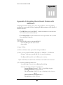
Appendix 3: Graphing Recruitment Chains with
NETDraw
Graphing recruitment chains can be done using NetDraw, a network graphing
program that comes with UCINet. Graphing an RDS recruitment chain requires 2
different data files:
1) The DL File, created with RDSAT, contains information on the structure
of the chains (who recruited whom).
2) The Attribute File contains information of the respondents and is created
from the RDSAT data file.
The DL File:
1) To create the file, load your data into RDSAT.
Select FileÆExport DL Network File
Save the file.
2) Open UCINet
3) Click on the Draw menu option. This will open NetDraw.
4) Once you have opened NetDraw (It should say “NetDraw – Visualization
Software” at the top, open the DL File you saved by selecting:
FileÆOpenÆUcinet DL text fileÆNetwork (1-mode)
Open the DL file you created. You should see a few red dots on the screen.
5) To view the recruitment chain select:
LayoutÆGraph-Theoretic layoutÆSpring Embedding
Select the following criteria in the popup box:
Layout Criteria: Distances + N.R. + Equal Edge Lengths
Starting Positions: Current positions
No. of iterations: 1000 (If you get overlapping chains, increase
this #)
Distance Between Components: 10
Proximities: geodesic distances
61
R D S
I N C O R P O R A T E D
Click “OK” and you should see your recruitment chains.
The Attribute File:
The attribute file is VERY similar to the RDSAT data file. To make it:
1) Open the RDSAT data file with Excel.
2) Replace “RDS” with “*node data” in the first line (all lower case, no space
between “*” and “node”, 1 space between “*node” and “data”)
3) Replace the sample size (row 2, column 1) with “Respondent ID”
4) Delete the columns of Coupon #s (since they are not needed)
5) Save the file as a “Tab delimited text file”, do not overwrite your RDSAT file.
6) Go back to NetDraw and select
FileÆOpen ÆVNA Text FileÆAttributes
In the popup, select the file you just saved and Select the “Node Attribute(s)”
bullet under “Type of Data”. Click “OK.”
7) Your attributes are now loaded.
8) NetDraw is almost completely interactive and fairly straight forward to use.
You can control individual nodes by clicking on them or groups of nodes by
using the popup menus on the side.
For example: select: Properties Nodes Color Attribute based. This will bring
up a popup box with a pull down menu with all your attributes in it. Selecting an
attribute will color code the node for that attribute.
A detailed discussion of the various features of NetDraw is beyond the scope of
this document.
62