Download learning kinetic monte-carlo simulator charles l. thornton a

A GRAPHICAL USER INTERFACE FOR THE SELFLEARNING KINETIC MONTE-CARLO SIMULATOR
by
CHARLES L. THORNTON
B.S., Kansas State University, 2003
A THESIS
submitted in partial fulfillment of the
requirements for the degree
MASTER OF SCIENCE
Department of Computing and Information Sciences
College of Engineering
KANSAS STATE UNIVERSITY
Manhattan, Kansas
2005
Approved by:
Major Professor
Virgil Wallentine
ABSTRACT
Kinetic Monte Carlo (KMC) is a non-deterministic computational technique for
simulating atomistic motion. These simulations can be used to predict the formation
of substances at the atomic level. This work describes a graphical user interface for
a variant of the KMC simulation technique called Self-Learning Kinetic Monte Carlo
(SLKMC) which is currently under development. We look at the SLKMC algorithm
as well as the steps users take to extract useful information from the simulation data.
Then we look at potential ways to enhance accuracy and productivity during the
model description and analysis phases of simulations. The user interface described in
this work includes support for the creation of initial condition data via mesh generation and global constant editing. It also provides improved support for simulation
results analysis. Analysis features include animated 3D model visualization and statistical data representation. The architecture and implementation of software designed
to carry out these enhancements is also discussed. We assess the usefulness of the
implementation of the software using reviews conducted by developers and users of
the SLKMC simulator. These reviews verify that the unified interface contributes to
both the usefulness of the underlying simulation code and user productivity.
Contents
List of Figures
iv
1 Introduction
1
1.1
1.2
KMC Background . . . . . . . . . . . . . . . . . . . . . . . . . . . . .
2
1.1.1
Kinetic Monte-Carlo . . . . . . . . . . . . . . . . . . . . . . .
3
SLKMC Technical Overview . . . . . . . . . . . . . . . . . . . . . . .
5
1.2.1
Running Simulations . . . . . . . . . . . . . . . . . . . . . . .
8
1.2.2
Validation . . . . . . . . . . . . . . . . . . . . . . . . . . . . .
12
2 Problem Description
14
2.1
Simulation Performance . . . . . . . . . . . . . . . . . . . . . . . . .
15
2.2
A Unified User Interface . . . . . . . . . . . . . . . . . . . . . . . . .
16
2.2.1
Simulator Input . . . . . . . . . . . . . . . . . . . . . . . . . .
17
2.2.2
Mesh Generation . . . . . . . . . . . . . . . . . . . . . . . . .
18
2.2.3
Problem Execution . . . . . . . . . . . . . . . . . . . . . . . .
19
2.2.4
Simulation Results . . . . . . . . . . . . . . . . . . . . . . . .
19
3 Software Description
3.1
23
KMC-Vis . . . . . . . . . . . . . . . . . . . . . . . . . . . . . . . . .
ii
23
3.2
3.1.1
Pre-Processing . . . . . . . . . . . . . . . . . . . . . . . . . .
25
3.1.2
Running the Simulation . . . . . . . . . . . . . . . . . . . . .
28
3.1.3
Simulation Analysis . . . . . . . . . . . . . . . . . . . . . . . .
29
KMC-Mesh . . . . . . . . . . . . . . . . . . . . . . . . . . . . . . . .
32
3.2.1
Mesh Creation
. . . . . . . . . . . . . . . . . . . . . . . . . .
33
3.2.2
Mesh Editing . . . . . . . . . . . . . . . . . . . . . . . . . . .
34
3.2.3
Mesh Visualization . . . . . . . . . . . . . . . . . . . . . . . .
36
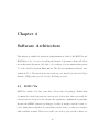
4 Software Architecture
4.1
4.2
4.3
38
KMC-Vis . . . . . . . . . . . . . . . . . . . . . . . . . . . . . . . . .
38
4.1.1
Data Model . . . . . . . . . . . . . . . . . . . . . . . . . . . .
39
4.1.2
Planned Scalability . . . . . . . . . . . . . . . . . . . . . . . .
42
4.1.3
3D Subsystem . . . . . . . . . . . . . . . . . . . . . . . . . . .
43
KMC-Mesh . . . . . . . . . . . . . . . . . . . . . . . . . . . . . . . .
45
4.2.1
KMC-Mesh Architecture . . . . . . . . . . . . . . . . . . . . .
45
Deployment . . . . . . . . . . . . . . . . . . . . . . . . . . . . . . . .
47
5 Results
50
5.1
User Acceptance . . . . . . . . . . . . . . . . . . . . . . . . . . . . .
51
5.2
Future Work . . . . . . . . . . . . . . . . . . . . . . . . . . . . . . . .
53
5.2.1
Enhancing KMC-Vis . . . . . . . . . . . . . . . . . . . . . . .
53
5.2.2
Enhancing KMC-Mesh . . . . . . . . . . . . . . . . . . . . . .
54
5.2.3
Extending the Core Simulation Code . . . . . . . . . . . . . .
55
A KMC-Vis Walkthrough
59
A.1 Overview . . . . . . . . . . . . . . . . . . . . . . . . . . . . . . . . . .
iii
59
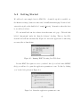
A.2 Getting Started . . . . . . . . . . . . . . . . . . . . . . . . . . . . . .
61
A.3 Opening a Main Configuration File . . . . . . . . . . . . . . . . . . .
62
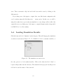
A.4 Loading Simulation Results . . . . . . . . . . . . . . . . . . . . . . .
63
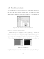
A.5 Simulation Analysis . . . . . . . . . . . . . . . . . . . . . . . . . . . .
64
B KMC-Mesh Walkthrough
67
B.1 Getting Started . . . . . . . . . . . . . . . . . . . . . . . . . . . . . .
67
B.2 Creating a Mesh
. . . . . . . . . . . . . . . . . . . . . . . . . . . . .
68
B.3 Saving Mesh Data . . . . . . . . . . . . . . . . . . . . . . . . . . . . .
71
C GUI Evaluation by Users
72
iv
List of Figures
1.1
Example of a KMC configuration . . . . . . . . . . . . . . . . . . . .
4
1.2
Example of a KMC process . . . . . . . . . . . . . . . . . . . . . . .
5
1.3
Pseudocode for simulation initialization . . . . . . . . . . . . . . . . .
6
1.4
Pseudocode for main simulation loop . . . . . . . . . . . . . . . . . .
7
1.5
The main configuration file (step16.dt) . . . . . . . . . . . . . . . . .
9
1.6
The databasefFile (baza c92)
. . . . . . . . . . . . . . . . . . . . . .
10
1.7
Database entry format . . . . . . . . . . . . . . . . . . . . . . . . . .
10
1.8
The initial configuration file (step16i.abk) . . . . . . . . . . . . . . .
12
1.9
Coalescence validation simulation results snapshots(from Rahman et.
al[1]) . . . . . . . . . . . . . . . . . . . . . . . . . . . . . . . . . . . .
13
2.1
Two symmetrical SLKMC processes . . . . . . . . . . . . . . . . . . .
21
2.2
Stack file format
. . . . . . . . . . . . . . . . . . . . . . . . . . . . .
22
2.3
Stack file format key . . . . . . . . . . . . . . . . . . . . . . . . . . .
22
3.1
Editing input options . . . . . . . . . . . . . . . . . . . . . . . . . . .
26
3.2
Validation of input options . . . . . . . . . . . . . . . . . . . . . . . .
26
3.3
Editing output options . . . . . . . . . . . . . . . . . . . . . . . . . .
27
3.4
The simulation execution view . . . . . . . . . . . . . . . . . . . . . .
28
v
3.5
The results view . . . . . . . . . . . . . . . . . . . . . . . . . . . . . .
29
3.6
Detecting process symmetries in KMC-Vis . . . . . . . . . . . . . . .
30
3.7
3D simulation history analysis . . . . . . . . . . . . . . . . . . . . . .
31
3.8
Low, medium, and high resolution atoms . . . . . . . . . . . . . . . .
32
3.9
KMC-Mesh screen shot . . . . . . . . . . . . . . . . . . . . . . . . . .
33
3.10 Creating a new mesh . . . . . . . . . . . . . . . . . . . . . . . . . . .
34
4.1
The data model used by KMC-Vis . . . . . . . . . . . . . . . . . . .
39
4.2
Use of the publisher-subscriber pattern in KMC-Vis . . . . . . . . . .
40
4.3
The publisher-subscriber pattern: Opening a configuration file . . . .
41
4.4
The publisher-subscriber pattern: Updating a button’s status
. . . .
41
4.5
Simulation execution data model . . . . . . . . . . . . . . . . . . . .
43
4.6
The 3D pipeline . . . . . . . . . . . . . . . . . . . . . . . . . . . . . .
44
4.7
The KMC-Mesh data model . . . . . . . . . . . . . . . . . . . . . . .
46
4.8
The JNLP file for KMC-Vis . . . . . . . . . . . . . . . . . . . . . . .
48
A.1 Running KMC-Vis using Java Web Start . . . . . . . . . . . . . . . .
61
A.2 Grant the application permission to run . . . . . . . . . . . . . . . .
61
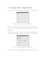
A.3 You will be greeted by a blank screen . . . . . . . . . . . . . . . . . .
62
A.4 The main configuration file editing view . . . . . . . . . . . . . . . .
62
A.5 The simulation execution view . . . . . . . . . . . . . . . . . . . . . .
63
A.6 The simulation results and analysis view . . . . . . . . . . . . . . . .
64
A.7 3D results view . . . . . . . . . . . . . . . . . . . . . . . . . . . . . .
64
A.8 Finding process symmetries . . . . . . . . . . . . . . . . . . . . . . .
66
B.1 Running KMC-Mesh using Java Web Start . . . . . . . . . . . . . . .
68
vi
B.2 Grant the application permission to run . . . . . . . . . . . . . . . .
68
B.3 The initial KMC-Mesh interface . . . . . . . . . . . . . . . . . . . . .
68
B.4 The mesh creation dialog . . . . . . . . . . . . . . . . . . . . . . . . .
69
B.5 An empty mesh . . . . . . . . . . . . . . . . . . . . . . . . . . . . . .
69
B.6 Filling the bottom layer with inactive atoms . . . . . . . . . . . . . .
70
B.7 A complete substrate . . . . . . . . . . . . . . . . . . . . . . . . . . .
70
B.8 A complete mesh . . . . . . . . . . . . . . . . . . . . . . . . . . . . .
71
C.1 Review from Altaf Karim . . . . . . . . . . . . . . . . . . . . . . . . .
73
C.2 Review from Abdelkader Kara . . . . . . . . . . . . . . . . . . . . . .
74
C.3 Review from Talat Rahmon . . . . . . . . . . . . . . . . . . . . . . .
75
vii
Chapter 1
Introduction
Physicists are increasingly using computational techniques to simulate the growth
of substances under different conditions[1]. Many of these techniques are complex
and sharing the underlying software tools is not always enough to share the process
itself. However, user interfaces allow us to control the level of detail presented to the
users, to provide graphical feedback to assist user input, and to optionally automate
complex analysis jobs – all without reducing the power of the underlying software.
This research explores a pre- and post-processor for a atomistic motion simulator
written in the FORTRAN programming language. The user interface was written in
Java and is completely separate from the computational software. Communication
is accomplished via the same text files the FORTRAN software uses to read input
and produce output. This means the physicists could continue work on their simulation code without having to learn a new programming language or worry about any
graphical techniques.
Development and adoption of the user interface was completely successful. In the
following chapters, we will discuss the specification, features, and architecture of this
1
work. Verification of the success of this project has come in the form of reviews by
users in the KSU physics department and their experiences with the software during
normal use and during a conference presentation. The full text of these reviews can
be found in Appendix C.
The particular technique used by the underlying software for modeling atomistic
motion is called Self-Learning Kinetic Monte-Carlo (SLKMC). This chapter discusses
the atomistic modeling concepts and some of the details of this particular implementation of SLKMC.
1.1
KMC Background
The branch of atomistic motion we are concerned with is the growth and movement
of a substance on a substrate. In order to produce materials according to certain
specifications, we must understand how individual atoms and atom clusters interact
with one another on a substrate. There are three approaches to modeling atomistic
behavior. Macroscopic modeling uses statistical descriptions of atomistic behavior to
simulate atom cluster movement[1]. Modeling can also be carried out at the atomic
level by methods that simulate the movement of individual atoms. There are also
hybrid models that attempt to combine macroscopic and microscopic techniques[2].
In this work, we are only concerned with a model that simulates the interactions and
processes of individual atoms.
Atomistic modeling has its roots in molecular dynamics (MD) simulations [3]. MD
simulations are based on Newton’s laws and are totally deterministic. The internal
computations are straightforward, but do not scale well to surface cluster modeling[1].
Techniques have been developed that allow researchers to focus on “interesting” mo2
ments in the evolution of a system when clusters of atoms begin to merge or separate.
One of these relatively young methods is Kinetic Monte-Carlo (KMC).
1.1.1
Kinetic Monte-Carlo
Kinetic Monte-Carlo simulations use a non-deterministic approach to model the movement of individual atoms on a substrate. The simulation proceeds in a series of
Monte-Carlo (MC) steps. At each step, the simulation selects one process to apply
to the model. A process (or transition) represents a transformation that the simulator will apply to a particular configuration of atoms, the energy threshold that
the transformation would have to overcome, and the change in time represented by
the application of the process . A configuration is a group of active atoms on the
substrate. When a configuration of atoms undergoes a process, the positions of the
atoms within that configuration are updated according to the rules defined in the
process.
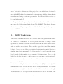
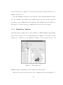
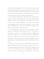
Figure 1.1 is an example of a configuration an a KMC simulation. In the KMC
model shown, the central atom has a 36 atom neighborhood arranged in a hexagon.
The empty circles represent locations in the configuration that could contain atoms
but do not; the dark circles represent other atoms within the configuration. The light
gray circles in Figure 1.1 represent the underlying substrate. Because the central atom
lies above the substrate in such a way that the substrate forms a triangle pointing
upward, this atom is said to be lying on an face-centered cubic (FCC) site – as well
as all of the other active atoms in this example. More complex models can represent
atoms lying on different kinds of sites within one configuration.
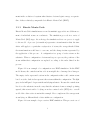
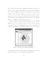
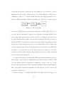
Figure 1.2 is an example of a process in a KMC simulation. This process is one of
3
Figure 1.1: Example of a KMC configuration
potentially numerous transitions the configuration in Figure 1.1 could undergo. The
arrow in this figure represents the movement the atom at its root will undergo. In
this particular example, the central atom will move along the edge of the other atoms.
It is not uncommon for many atoms to move in a particular process.
At every MC step, a process is selected in a weighted-random fashion based on
the energy thresholds of each potential process in the simulation. This process will
transform a small portion of the model and then the next process will be selected.
As there is no notion of convergence, the simulation will run until a desired number
of MC steps have been calculated.
As the atoms shift their positions, the cluster shape, its energy, and dynamics
change. Tracking these changes is one of several ways to analyze atomistic simulations.
Using this information, scientists can learn how different materials form and how to
create desired behaviors.
The constant motion of these entities prevents the stagnation found in the older,
4
Figure 1.2: Example of a KMC process
more rigid atomistic models. Unfortunately, this comes at the price of higher computational complexity and the need to specify more accurately the details of the system.
Efforts are continually underway to refine existing KMC approaches by increasing the
resolution of the computational model. The validation section later in this chapter
discusses a coalescence problem used to verify the version of KMC underlying this
research.
1.2
SLKMC Technical Overview
In order to understand the flow and data structures used by SLKMC, it is first
necessary to define a few terms.
Definition: Let HashSet be a data structure with the following properties:
• Maintains a list of Key → V alue pairs
• Provides get and put methods which access and modify the data structure
5
• Does not allow duplicate keys
• Each V alue in the HashSet is a non-empty Set of values
Definition: Let a Conf iguration be the arrangement of a central atom and its 36
neighboring sites.
Definition: Let a T ransition be the triple of initial configuration, energy threshold,
and end configuration.
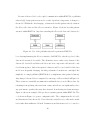
With those definitions it is possible to describe the behavior of the SLKMC software. Note that many other things are going on in the simulation, but these algorithms capture the core of the SLKMC implementation. Figure 1.3 shows pseudocode
for the algorithm that initializes the simulation. In essence, initialization simply popLet tTable be an empty HashSet
Let A be the set of all active atoms in the simulation
for each atom a in A
T = getPossibleTransitions( a )
for each transition t in T
add the mapping (t, a) to tTable
Figure 1.3: Pseudocode for simulation initialization
ulates the process list (tT able) with all of the possible processes that can occur.
Because tT able can map a single key (or transition) to many values (in this case
atoms), the important data are the processes – not the central atoms. It is done in
this way because we calculate the probability of a process independent of how many
places it can occur. We will discuss the getP ossibleT ransitions function later.
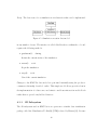
Once the simulation has been properly initialized, the main loop will repeat until
the desired number of MC steps have been calculated. Figure 1.4 shows pseudocode
for the main simulation loop. At each MC step, we select a weighted-random tran6
Let transition chosenTrans = getWeightedRandomTransition( tTable )
Let atomList = tTable.get( chosenTrans )
Let centralAtom be a random atom from atomList
perform chosenTrans on centralAtom’s configuration
for each active atom a in centralAtom’s configuration
remove all mappings to a from tTable
ts = getPossibleTransitions( a )
for each transition t in ts
add (t, a) to tTable
Figure 1.4: Pseudocode for main simulation loop
sition from our table of possible transitions. The weighting is determined by the
energy threshold of that transition. Once we have a transition, it is possible to extract the list of atoms whose configurations are valid candidates for that transition
from tT able. A random atom (and its respective configuration) is selected from the
list of candidate atoms. That configuration is transformed and the transition table is
updated to reflect the new configuration.
In both pseudocode examples, the getP ossibleT ransitions function was invoked.
This function is the subject of scrutiny in the project because it is responsible for most
of the up-front computation and often much of the time consumption. If a particular
configuration has already been seen in the simulation, getP ossibleT ransitions will
simply return the set of transitions that can be applied to the configuration. This
behavior is the “Self-Learning” aspect of SLKMC. It is very powerful because there
are only a finite number of configurations, and even fewer reasonable configurations.
The database used to maintain information about past configuration to transition set
mappings can also be reused between simulations, so this presents an excellent opportunity to avoid the expense of the external function used to calculate the transition
set for unknown configurations.
7
If a configuration shows up that has not previously been seen in the simulation,
it is necessary to invoke an external function to calculate the possible transition set.
This function uses techniques described in [1] and I will not discuss them in detail
here. The external function calculates all of the possible transitions that could arise
from a particular configuration and it inherently takes a long time (on the order of
minutes) to execute[7]. The accuracy of the entire simulation is dependent on the
resolution of this calculation. Unfortunately, this resolution is directly proportional
to external function execution time.
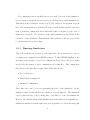
1.2.1
Running Simulations
This section will give an overview of each required file. It is not intended to serve as
a complete user’s manual for the SLKMC software. To run a SLKMC simulation, the
user must create four files. A top-level configuration file provides some global values
and provides the names of other configuration and results files. This configuration
file references the other three required files. These files are the:
• Process Database
• Initial Mesh Configuration
• Substrate Configuration
These three files can be seen as representing the state of the simulation. As the
simulation runs, checkpoint files are output at a preset interval. The simulation
can be rerun from any of these checkpoints, or modified to create new simulations.
However, since Kinetic Monte-Carlo simulations are inherently non-deterministic, two
simulations initialized from the same state are not guaranteed to follow the same path
8
or reach the same final state. Even though the main configuration file provides an
initial random number generator seed, there is not currently any way to capture the
state of the internal random number generator at each checkpoint.
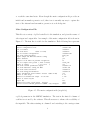
Main Configuration File
This file sets a variety of global variables for the simulation, and gives the names of
other input and output files. An example of the main configuration file is shown in
Figure 1.5. The first line is a title for the simulation. Each following line represents
KINETIC MONTE_CARLO ,STEP16m ,ON Cu/CU111 11/11/2003 new gen
initial configuration file
clust9i.abk
file of results
clust92.r
file with movie
(name or none)
clust92.m
file for result configuration
clust92f.abk
file with config database
baza_c92
output sample for NEB and current config
no
update database
yes
analysis of 3d index in pattern recognition
no
file for output event_stack ( name or none)
stack_c92
output of config
( yes or no
)
yes
file with control parameters output
clust92.con
file with substrate config for NEB
cu111r.sub
file with event statistics
clust92.st
file with energy distribution
clust92.en
output information about nonzero classes (YES or NO)
yes
number of time steps
1.e7
interval of information output in one run
1.1e4
number of static layers
2.
temper (K)
500.
interval for event_stack output (<10000)
9000.
initial seed for random generator (ISEED - any integer)
6543.
Figure 1.5: The main configuration file (step16.dt)
a global parameter in the SLKMC simulation. The text in the first 60 columns of
each line is not used by the software. This allows users to enhance the readability of
the input file. The values starting at column 61 and extending to the carriage return
9
are read in a specific order by the simulation software. Notably, this configuration
file references “clust9i.abk” as an initial configuration file, “baza c92” as a database
file, and “cu111r.sub” as a substrate configuration file. These are the three required
additional input files and we will briefly discuss each one.
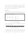
Database File
This file maintains the running record of all calculated database processes. A portion
of an example database file is shown in Figure 1.6. The first four lines allow the user
baza for 7 atom at 500K cluster 7/1/2004
35
32
37
7
59
14
...
2051
3073
2051
22
32
40
0
196608
0
0
0
128
1
1
1
0
1
1
0.670
0.052
0.312
1
1
1
1
1
1
4
2
3
0.322
0.647
4
1
1
1
4
2
2
3
3 11
7
1
Figure 1.6: The databasefFile (baza c92)
to insert comments describing the database and the simulation it was used in. The
entry format is shown in Figure 1.7.
shellA
shellB
shellC
∆E i
n
mi
posjinit
posjf inal
Figure 1.7: Database entry format
The first three entries (shellA , shellB , shellC ) in each line of the database refer
to a particular configuration of an atom cluster. Binary encoded integers are used
for this representation to conserve space. The next entry (n) gives the number of
10
different processes that can occur from that particular configuration. Each process is
fully described by the following entries. The entry ∆E i is the threshold energy for the
ith process. The entry mi is how many atoms within the shell configuration moved
in the process. The value of mi will always be non-zero. For each moving atom, we
have an initial location and a final location. These are given as posjinit and posjf inal
respectively. Notice that no value is given for the duration of a process. The same
process can be applied over different periods of time.
Process descriptions are appended to the database any time the external function
is required to generate them. If a simulation is run using an initially empty database
file, a large part of the initial runtime is devoted to building up the database. However,
two simulations with a common substrate configuration can share a database file. In
theory, this would allow the databases to be linked to the substrate configurations in a
technique that would eventually give a “complete” database. However, this technique
has not yet been fully explored. Unfortunately, more complex models make exploring
the configuration state space an increasingly difficult problem.
Initial Configuration File
This file provides the simulator with the starting locations of each substrate atom
and active atom. A portion of an example initial configuration file is given in Figure
1.8. The first three lines in the initial configuration file allow users to add suitable
documentation to the file. They are not used by the simulation software. Each
following line represents a single atom in the simulation. The first three fields contain
floating-point values that describe the position of the atom in R 3 . The next three
fields describe a velocity vector for the atom. In the initial configuration file, this
velocity vector is always zero. The final field is a flag to indicate that an atom is
11
INITIAL CONFIGURATION
102.2476
88.54905
1600
3
0.00000
0.00000
1.27810
2.21373
2.55619
0.00000
...
3214
8.348480
0.00000
0.00000
0.00000
14
0
0.
0.
0.
0.
0.
0.
0. 0
0. 0
0. 0
Figure 1.8: The initial configuration file (step16i.abk)
either “active” or “inactive”. Active atoms use a value of ‘1’ for the flag. They will
be moved around by simulation processes. Currently, active atoms only reside on
the top layer (above the substrate atoms). Inactive atoms use a value of ‘0’. They
represent the substrate and occupy the lower two layers of the simulation – in a three
layer model.
Substrate Configuration File
This file provides the previously mentioned external function with information about
the current substrate. Its format is identical to the initial configuration file. The only
noteworthy difference between this file and the initial configuration file is that the
velocity vectors are frequently non-zero in the substrate configuration file because of
the molecular dynamics equations used in that computation.
1.2.2
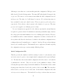
Validation
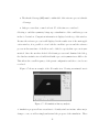
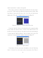
The SLKMC software has been validated against experimental data in a coalescence
simulation. In this simulation, a large island of atoms is placed near a smaller island
of atoms. In time, the smaller island will merge with the larger one[5]. Figure 1.9 is
a visual history of this simulation. The results of this validation are exciting because
12
Figure 1.9: Coalescence validation simulation results snapshots(from Rahman et.
al[1])
they agree with previously collected experimental evidence[1]. A detailed discussion
of the validation simulation can be found in Rahman et. al[5].
13
Chapter 2
Problem Description
The existing Self-Learning Kinetic Monte-Carlo (SLKMC) software is evolving in
three key areas:
• Simulation Accuracy
• Simulation Performance
• Usability
Efforts to increase simulation accuracy by increasing model resolution are continually underway. In order to provide suitable performance for finer-grained simulations,
optimizations are needed both in results data size and simulation running time. Current simulations produce 1-3 gigabytes of data, and take hours to run. This time can
extend to weeks if the process database must be discovered by the system. Usability
is important if we intend to share not only the simulation results, but the process
itself. Other scientists will find it much easier to pick up a simulation package if they
do not need to concern themselves with the details of file formats, or are forced to
recompile the software to make minor changes.
14
A key idea in this project is that physicists should continue to develop and maintain the core computational engine within the SLKMC software. Their backgrounds
give them tremendous insight into the underlying problem and shifting ownership of
the code into the hands of computer scientists for greater convenience in enhancing
performance and usability would not be ideal. For this reason, the coupling of any
software modules that address either of the second two areas must be very loose. The
remaining sections in this chapter will discuss areas of the SLKMC software that need
to be improved. This thesis focuses on the effect of enhancing the software usability,
thus usability improvements are given considerable emphasis.
2.1
Simulation Performance
The development of more accurate simulation technology is entirely dependent on
the performance of the system. Currently, the accuracy of SLKMC is fully scaleable,
but growth in this area is stunted because simulations can take weeks to run. From
the main simulation loop described in Chapter 1, we can isolate the two performance
bottlenecks in the software.
The first in computation of the external function. Calculating the possible processes
that a particular configuration can undergo takes a matter of minutes with the present
computing technology. The good news is, this computation never needs to be repeated
for a particular configuration. This is the “Self-Learning” nature of SLKMC – as the
database grows, the external function is needed less often. One technique that is
currently being applied to this problem is pattern recognition[1].
In the 36-neighbor configuration model demonstrated in this work, it is possible
to simply explore the entire configuration space and add each mapping to the process
15
database. Pattern recognition schemes can be used to greatly reduce the space via
configuration symmetries. This reduction will become invaluable in the next generation of SLKMC which will use a 210-neighbor configuration model. Some pattern
detection technology currently exists in the software, but a project is underway to
add far more sophisticated artificial intelligence to the pattern recognition engine. It
is also important to mention that the symmetry detection must be perfect since even
a small margin of error expanded over billions of Monte-Carlo steps would seriously
degrade simulation accuracy. Assuming an effective system was in place, no amount
of symmetry detection could prevent occasional calls to the external function. For
this reason, work is being done to parallelize the simulation.
Combinations of pooled and distributed technologies have been considered to
off-load the computation of potential processes[8]. Because the computation of the
process list for a particular configuration is both extremely expensive and completely
independent of other computations it is a natural candidate for distribution. However, as previously discussed, being forced to compute the external function is ideally
a temporary problem. The long-term goal of any parallelization effort must be to improve the performance of the individual time steps. An interesting approach currently
being explored is to execute parallel updates localized to particular atom clusters[6].
This technique promises to overcome the inherently serial nature of the single process
per MC step simulation at the cost of very complicated division of labor.
2.2
A Unified User Interface
From a user’s perspective, there are three important tasks when running a simulation. The first is to describe the problem to the simulator. This is accomplished by
16
generating the input files discussed in Chapter 1. The second step is to actually run
the simulation and await the results. As the simulation is running, data is being generated. Once the user has the required data, the results must be analyzed in a useful
way. The following sections will discuss different elements of those three processes.
2.2.1
Simulator Input
A problem description consists of four input files:
• main configuration file
• substrate configuration file
• initial mesh configuration
• process database (substrate specific)
In general, the substrate configuration file and the process database can be reused
from existing sources. Because the KMC project has not yet advanced to a point
where users are creating custom substrates, both of these files are assumed to predate
the simulation. The pre- and post-processing software is then focused on the main
configuration file and the initial mesh configuration.
The main configuration file is a plain text file consisting of a number of key value
pairs. While any user with a text editor can manipulate this file, there are a number
of problems with generating input in this way. The first problem has to do with
assumptions. Without a knowledge of the underlying software system, a user might
assume that the input file was actually a sequence of key-value pairs. This is not the
case. The first sixty characters of each line provide a description of possible values
to guide the user, but these values are read by the simulator which assumes they are
17
in the proper order. Even more disturbing is the realization that once the proper
ordering of these lines is lost, it could require a backup example or a knowledge of
the underlying code to repair the error.
Another issue when directly interacting with the text file is validation. Details
like the valid width and format of floating-point values, entering boolean values, and
knowing what strings are valid input all require thorough documentation and experience to avoid potentially time-consuming headaches. Also, simple typographical
errors can occur in directly edited text files.
A final complaint against direct text editing is presentation. Issues such as logical
grouping and warning against underdeveloped options can only be addressed in the
most rudimentary fashion within rigidly defined text input file. However, techniques
are available to address all of these issues with a modern graphical user interface.
2.2.2
Mesh Generation
In the main configuration file, each entry represented a conscious decision by the user.
This does not hold true for the mesh configuration file. It is not realistic to expect
a user to enter the locations of every atom in a 30x50x3 grid by hand (4500 lines
of numerical text). In determining the initial configuration for a simulation, users
should be able to provide a higher level description of a mesh, then have a tool build
it for them. Tools such as this predated my research, but there were a number of
features that did not yet exist.
Users wanted the ability to populate meshes using pre-existing “island” patterns[7].
Ideally there would be a library of predefined islands that could be drawn from and
added at particular locations, or new shapes could be created. Features that allow
18
creative control over the positions of individual atoms create a new layer of functionality that wasn’t present in existing tools. They also require some form of visual
feedback for the placement of the atoms.
2.2.3
Problem Execution
Once the correct input files are in place, running the simulation is quite simple. A
compiled, executable version of the KMC software will seek out the input files in the
working directory, read in the data, and run the simulation. Invalid input files will
cause the simulation to prematurely halt. As the simulation runs, results data is
continuously written to output files. This data can be analyzed either immediately,
or after the simulation is finished. This approach is straightforward, but it has some
limitations related to parallelism and usability.
There are two unavoidable problems that will occur when running a KMC simulation. The first is a heavy CPU load, and the second is the amount of output that
will be generated. The computational load is a product of the algorithms described
in Chapter 1. The volume of output data is proportional to the number of MC steps
requested in the simulation. Small simulations produce hundreds of megabytes of output, large simulations produce gigabytes. Ideally, we want a way to execute problems
quickly, without losing the ability to analyze results as they become available.
2.2.4
Simulation Results
From the standpoint of results, a KMC simulation is a stream of processes applied to
particular atoms. This information can be used in several ways:
• Visualizing the motion of atom clusters
19
• Analyzing the process statistics to “explain” the simulation
• Numerical analysis of the motion of the atom clusters
Meaningful data is collected using a combination of these three techniques. The
following sections will discuss the use of each of these techniques and the challenges
that must be addressed for the KMC software to be more useful and accessible.
Visual Simulation History
Despite the constant motion of a KMC simulation, the key moments occur during a
relatively small fragment of the simulation timeline[7]. It is important to be able to
monitor the simulation in a way that allows researchers to view progressively finergrained data and identify these important moments. The mechanism used for this
purpose (prior to this research) was a “movie” file that contains the positions of the
active atoms within the simulation. The position of each active atom was written
to the movie file after a number of MC steps specified in the main configuration
file. Unfortunately, this system fixed the granularity of movie output for an entire
simulation. Unless the user guesses correctly the first time, finer granularity could
only be obtained via additional executions of the software.
Process Statistics Analysis
There are a variety of different types of database processes. Rahman, et al[5] contains
a listing of 27 unique process variants discovered in a single experiment. Identifying
what kind of processes the system underwent and their frequency acts as an explanation for the changes that occur within the simulation model during the key moments
described above.
20
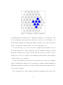
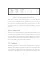
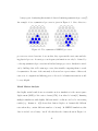
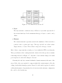
A major part of analyzing this statistical data is identifying symmetrical processes[7].
An example of two symmetrical processes is given in Figure 2.1. Since these two
Figure 2.1: Two symmetrical SLKMC processes
processes are rotated versions of one another, they represent the exact same underlying physical process. Accurate process frequency information can only be obtained by
coalescing symmetrical processes into individual, unique processes. Analysis is carried
out by building a list of all common processes, then visually comparing them to search
for symmetries. Because of the extremely tedious and error prone nature of this work,
some sort of computational filtering prior to the need for human intervention would
be very helpful.
Island Motion Analysis
One highly useful result from an atomistic motion simulation is the mean square
displacement (MSD) of the center of mass (CM) of an island of atoms[1]. Running
multiple simulations with slightly different initial conditions can lead to interesting
results (e.g. Raman et. al[1] shows that clusters displace at dramatically different
rates when they contain different numbers of atoms). In SLKMC simulations, this
data is tracked via a binary “stack” file that has the format shown in Figure 2.2.
21
A description of each of the fields in the stack file are given in Figure 2.3. In this
∆t
katom
n
posinit
1
posf1 inal ... posinit
n
posfninal
Figure 2.2: Stack file format
representation, the byte length of floating-point data is 8 bytes, and the length of
∆t
katom
n
atomi
posi
(real) Elapsed time during this Monte-Carlo step
(real) Central atom’s position in k-space
(int) Number of moving atoms
(int) Initial position of the ith moving atom
(int) New position of the ith moving atom.
Figure 2.3: Stack file format key
integer data is 4 bytes. Entries in this stack file are written out every time step and
custom data reader software has been created to perform analysis on the data. After
growing for millions of MC steps, this simulation stack file becomes quite large.
Custom readers for the file format have been written by the developers of SLKMC,
but they do not allow users to target particular interesting portions of the data.
Ideally, users should be able to plot the MSD for an island at the particular time
window that is significant for the simulation without resorting to trial and error.
Also, it would be very helpful if users were allowed to perform different calculations
on this step-wise data to generate a variety of graphs.
22
Chapter 3
Software Description
3.1
KMC-Vis
This chapter will discuss the features in an application designed to address many
of the productivity and usability issues raised in previous chapters. The software is
called KMC-Vis because it represents a visual interface to the KMC package. The
objective of KMC-Vis is to allow a user to prepare, execute, and analyze an atomistic
simulation all within a single program. Following that assumption, there are a several
important guiding characteristics:
• It must be possible to run all data preparation and analysis tools from within
the KMC-Vis interface.
• KMC-Vis will be the client in a client-server architecture. A high-performance
simulation server will handle computation.
• To accommodate the scientific community, the software must run on both Linux
and Windows operating systems.
23
• Retrieval and execution of the client application via the Internet must be as
simple as possible.
The remainder of this section will discuss each of these features and how KMC-Vis
addresses them. Following sections provide details on the different components of the
user interface. A tutorial for KMC-Vis is available in Appendix A.
Prior to this work, their were a variety of FORTRAN programs written by the
designers of SLKMC. These programs allow their authors to automate some of the
pre- and post-processing tasks involved in a simulation. Unfortunately, while this
system brings enormous power to a small group of developers, it creates a very sharp
learning curve for new users. KMC-Vis is intended to be a single application that
brings together all of the tools that the simulation software users need in such a way
that their use is intuitive. The implementation of KMC-Vis in this research represents
a first pass at this goal, and was intended to demonstrate the feasibility of such a
project. Due to time constraints on this phase of the project, it is not possible for
the user interface to provide complete functionality.
A pressing issue is the performance of the SLKMC simulation engine. Research
is underway to apply a parallel solution to this performance problem. Since most
users do not work on a multi-processor computer, it has been predicted that the
final system will be a client-server style architecture with the server commanding the
power of many computational nodes. The client software must then submit work
and retrieve results from the server. KMC-Vis represents the client element of this
architecture.
In recognition of the increasing popularity of the Linux operating system, KMCVis would ideally be available to users of both Windows and Linux-based operating
24
systems. This is easily accomplished using a cross-platform language such as Java.
In order to smooth over interoperability issues in the future, C++ may become a
language of choice, and in that case a multi-platform toolkit for 3D visualization and
windowing would be ideal.
The client software has been designed to make it as easy as possible to launch
via the web. Because mature versions (those that interact with a simulation server)
will require an Internet connection, this does not impose any penalties and enhances
usability. Java applications can take advantage of Java Web Start technology which
allows the software to install and run with a single click. Installers would have to be
created for other forms of the client software.
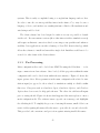
3.1.1
Pre-Processing
Main configuration files can be loaded into KMC-Vis using the File|New... technique common in modern software. Once loaded, all the properties within the main
configuration file can be edited from within the user interface. Figure 3.1 shows the
input options editor. Every parameter in the main configuration file related to simulation input (as opposed to those related to simulation results) is editable within
this view. Categories such as Simulation Input, Simulation Options, and Database
Options have been created to help guide the user. The editor also validates all inputs
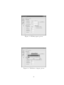
prior to saving the file. Figure 3.2 shows what happens if the user neglects to enter a
mesh configuration file. The software issues a specific error message, and highlights
the offending field. To simplify the process of entering file names, small folder icons
next to fields requiring file names allow the user to open a file chooser and select a file.
This provides both convenience and protection against entering invalid file names.
25
Figure 3.1: Editing input options
Figure 3.2: Validation of input options
26
A button labeled “Run KMC-Mesh” can be seen among the input options. KMCMesh is a program specifically designed to assist in the creation of initial mesh configuration files (those ending with .abk). KMC-Mesh can be executed from within
KMC-Vis or as a stand-alone application. Section 3.2 will cover this tool in more
detail.
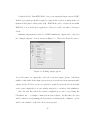
Similarly, all parameters related to a KMC simulation’s output can be edited via
the “Output Options” view as shown in Figure 3.3. This view allows the user to
Figure 3.3: Editing output options
choose file names for output files, and select optional output options. Validation
similar to that found in the input options view protects the user from entering invalid
output options. Folder icons are not present to assist the user’s file selection in this
view because output files do not necessarily exist prior to execution of the simulation.
Once the user has edited the current configuration, it can be saved using the
File|Save As... technique common in modern software. At this time, the data
will be validated and (assuming the data survived validation) the “Simulate” option
will become available on the left editor selection panel.
27
Notably absent from the pre-processing feature list is creating three of the four
required files from scratch. This support has not been included in the version of the
code discussed in this work. Clearly, this feature is important and must be added
before the client software is ready to be used outside the KMC research group. Section
5.2 discusses this and other future work for the project.
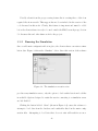
3.1.2
Running the Simulation
Once a valid main configuration file is in place, the client software can retrieve simulation data. Figure 3.4 shows the “Simulate” editor. Since this version of the software
Figure 3.4: The simulation execution view
pre-dates any simulation server, only the option to load results data from local files
in available. Options designed to assist the user in connecting to a simulation server
are left disabled.
Clicking the button labeled “Start” (shown in Figure 3.4) causes the software to
attempt to load data from the database and results files listed in the main configuration files. Attempting to load data that does not exist will result in an error.
28
Progress messages are displayed to keep the user informed during what may be a
lengthy loading process.
Once the simulation database is loaded and the other results information is available, the “Results” option will become available in the left editor selection panel. It
is possible to view results while only a fragment of the simulation data is available to
allow users to track the progress of simulations and view data as it emerges.
3.1.3
Simulation Analysis
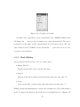
Progressively more results data becomes available as a KMC simulation runs. KMCVis provides two major modes of analyzing this data. Figure 3.5 shows the top-level
results view. Database process analysis is available on the top-level screen. 3D
Figure 3.5: The results view
simulation history visualization is also available in a sub-window.
Database processes are presented in a tree configuration as shown in Figure 3.5.
29
The roots of these trees are the atomic configurations from which processes may occur.
One level down is a complete list of transitions (or processes) that were initiated by
the root atomic configuration. Only those processes that have occurred during the
simulation are listed. The shown configurations are ordered by the frequency of their
aggregate processes. Because there is no natural labeling other than that applied by
a human analyst, the most meaningful label available for the tree is the aggregate
frequency of a configuration, or the frequency of a process.
One time consuming research task is identifying symmetrical processes. KMC-Vis
implements a novel tool to assist in the discovery of such processes. By selecting a
process, then clicking on the “Find Symmetries” button, a user can launch the symmetry detection tool (Figure 3.6). Within the symmetry detection tool, the reference
Figure 3.6: Detecting process symmetries in KMC-Vis
process is indicated at the top of the process list, and candidate processes are listed
underneath. Candidates are selected using the following qualifications:
30
• The threshold energy (∆E) must be within 0.01 of the reference process’s threshold energy.
• Only processes that occurred at least 1% of the time are considered.
Selecting a candidate symmetry brings up a visualization of the candidates process
in the tool’s window. Comparison information is displayed at the top of the window.
Because the reference process is still displayed in the results view of the main application window, it is possible to view both the candidate process and the reference
process at the same time. A checkbox can be clicked to specify that a process is symmetrical. Once the user has checked all relevant processes and dismissed the dialog,
the database statistics tree rebuilds itself with a process’s symmetries as child nodes.
This affects the overall frequency of the parent configuration and the root nodes are
reordered.
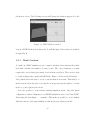
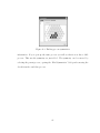
Figure 3.7 shows an example of the 3D results view. Viewing an animated movie
Figure 3.7: 3D simulation history analysis
of simulation progress allows researchers to identify windows in time where major
changes occur, as well as simply understand the progress of the simulation. These
31
windows help to focus other types of analysis such as center of mass tracking. Movielike buttons such as stop, play, and step are available to allow the user to easily move
back and forth through the simulation movie.
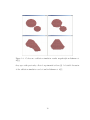
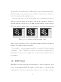
Users have full control over the viewing angle and zoom within the 3D window.
It is also possible to change the resolution of the atoms in the movie. Figure 3.8
shows the difference between the low, medium, and high settings for atom resolution.
The lowest available setting allows low-end machines to render the 3D visualization
Figure 3.8: Low, medium, and high resolution atoms
with acceptable performance, where as the highest setting is useful for presentation
graphics. The default resolution is medium.
It is possible to export presentation graphics of a particular 3D scene using the
“Save Image...” button. This will open a file chooser where users can name and save
their images. Atom sizes can be adjusted via a drop-down menu similar to the one
for resolution.
3.2
KMC-Mesh
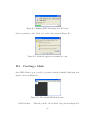
KMC-Mesh is a mesh generation program available as either a stand-alone application or from within the KMC-Vis software. It allows users to create and modify
configurations of atoms in a visual interface. Figure 3.9 is a screen shot of the ap32
plication in action. The following sections will discuss the features supported by the
Figure 3.9: KMC-Mesh screen shot
version of KMC-Mesh used in this work. A walk-through of the software is available
in Appendix B.
3.2.1
Mesh Creation
A “mesh” in a KMC simulation is two complete substrate layers underneath a third
layer that contains some number of active atoms. The correct definition of a mesh
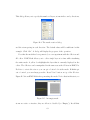
requires the correct relative placement of each atom in every layer. There are two ways
to begin working with a mesh in KMC-Mesh. Figure 3.10 shows the File|New...
dialog which allows the user to create a custom mesh from scratch. This method of
mesh creation allows the user to specify the atom spacing and the number of atoms
in the x, y, and z (layers) directions.
It is also possible to work with an existing simulation mesh. Any valid initial
configuration or final configuration of a SLKMC simulation can be loaded into KMCMesh using the File|Open... command. This makes it possible to create slightly
different versions of the same simulation without directly editing a text file.
33
Figure 3.10: Creating a new mesh
Any time a user would like to create a mesh suitable for a SLKMC simulation the
File|Save As... option provides a simple way to write the mesh files. The user is
prompted for a file name, and the current mesh is stored at that location. Since the
same format is used by SLKMC and the File|Load... option, there is no need for
a separate export function.
3.2.2
Mesh Editing
Any atom in the mesh can have only one of three states:
• Empty/Disabled
Disabled atoms will be ignored at file write time
• Inactive
Inactive atoms will be written at file write time with active flag value “0”.
• Active
Active atoms will be written at file write time with active flag value “1”.
Editing a mesh is manipulating the activity state information for the atoms within a
mesh. To support this function, the mesh editor view (right hand side of Figure 3.9)
34
provides several tools:
• Layer Up
Changes the current editing layer to the next available layer in the z + direction.
This option is disabled when the top layer is selected.
• Layer Down
Changes the current editing layer to the next available layer in the z − direction.
This option is disabled when the bottom layer is selected.
• Reset View
Resets the zoom and drag settings to the defaults.
• Zoom In
Increases the zoom factor within the editor view.
• Zoom Out
Decreases the zoom factor within the editor view.
• Drag Tool (Default)
Allows the user to translate the editor view. This is convenient when the current
zoom obscures portions of the current layer.
• Make Layer Inactive
Sets all cells in the current layer to the “inactive” state. This is useful for
creating substrate layers.
• Make Layer Empty
Sets all cells in the current layer to be ignored.
35
• Empty Atom Tool
Allows the user to set individual atoms to the “empty” state.
• Inactive Atom Tool
Allows the user to set individual atoms to the “inactive” state.
• Active Atom Tool
Allows the user to set individual atoms to the “active” state.
These tools allow the user to quickly create custom simulation configurations without
ever looking at the mesh configuration input file.
3.2.3
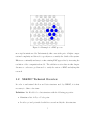
Mesh Visualization
As the user edits the mesh in the editor view, those changes are immediately applied
to the mesh visualization shown in the left of Figure 3.9. This view provides a 3D
representation of active mesh. Atoms in the mesh are color-coded according to state.
Active atoms are yellow, inactive atoms are blue, and disabled atoms are shown in
a semi-transparent white. This side-by-side arrangement provides the user with a
sense of perspective and orientation while working with a mesh. Users have complete
control over the camera position and zoom factor used in the 3D view via the mouse.
A “Reset View” button is available on the toolbar to return the camera and zoom to
its default position.
Another feature of the 3D view is a highlighted box indicating the current editing
layer. As the user changes the editing layer using the “Layer Up” and “Layer Down”
tools within the layer editor, a translucent yellow box travels up and down the visualization indicating the selected layer. This option can be toggled on and off using a
36
toolbar button.
37
Chapter 4
Software Architecture
This chapter is a high-level discussion of implementation details of the KMC-Vis and
KMC-Mesh tools. A section describing the Internet deployment scheme will follow
the architectural discussion. All of the code for this project was written using version
1.5 of the Java Development Environment. The 3D data visualization libraries were
written in C++. The interaction between the two was handled via the Java Native
Interface (JNI) package provided by the 3D library provider.
4.1
KMC-Vis
KMC-Vis consists of 66 Java source files collected into six packages. Rather than
document the detailed interactions between each of these files, this section will discuss the data model used by the software and explain the communication paradigm.
Because the SLKMC software is a living project (the 36 neighbor version became obsolete during this work), there are particular portions of the code that were designed
with scalability in mind. This section will focus on those places in the software ar-
38
chitecture. Finally, the 3D subsystem used in KMC-Vis is the same as the one used
in KMC-Mesh. A section is dedicated to explaining that system.
4.1.1
Data Model
The data model contains all of the data needed to write out the supported input
files, keep track of simulation progress, and analyze the results. Data internal to
KMC-Vis such as the preferred window size is also maintained in the data model, but
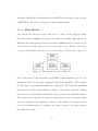
in the interest of clarity will not be described in this section. Figure 4.1 shows an
overview of the runtime data model used by the software. The model is composed of
Figure 4.1: The data model used by KMC-Vis
three components: Config, Run Data, and Results. Config maintains a record of all
information related to the main configuration file for the simulation. This includes
the file names of the simulation input and output files. The Run Data maintains
information about the current simulation status. Notably, this component contains
the data source for the simulation that will be used to generate the results information.
The results section of the model contains the mesh and movie data. Strangely absent
from the results data is the simulation database. The database is actually stored at
the top level within the model. Statistics are applied directly to the database when
the results are read in.
39
Because of the need for loosely coupled communication within KMC-Vis, a publishersubscriber[9] design pattern was used to notify dependent components of changes to
the model. Within the Java language, a framework for this pattern already exists in
the Observable class and the Observer interface. Figure 4.2 shows how this pattern
was used within KMC-Vis. Any class extending the Observable class can be listened to
Figure 4.2: Use of the publisher-subscriber pattern in KMC-Vis
by a class implementing the Observer interface. In KMC-Vis, only the top level of the
data model was made observable. The alternative was to make every element of the
data model observable and then each editor and view component could subscribe only
for relevant updates. Such a fine-grained solution would be very desirable if the data
model were frequently changing, but this performance benefit never outweighed the
simplicity of a single publisher (KMC-Mesh does implement a fine-grained solution).
Any change to the model is accompanied by a message or Event as listed in Figure 4.2.
These events are essentially an enumeration within the kmcvis.model.Event class. By
refraining from updating after irrelevant events, subscribers can significantly reduce
any performance penalty they may have incurred from hearing irrelevant messages.
Figure 4.3 shows an example of the producer-consumer pattern within KMC-Vis. The
code shown in Figure 4.3 opens a configuration file. The configuration file is loaded
and then inserted into the model. Notice that the notifyObservers call is made at this
level rather than within model itself. If numerous modifications need to be made to
40
URL res = jfc.getSelectedFile().toURL();
Config cfg = Config.load(res);
Model.getModel().setConfig(cfg);
Model.getModel().notifyObservers(Event.CONFIG_OPEN);
Figure 4.3: The publisher-subscriber pattern: Opening a configuration file
the model at the same time, this technique prevents a serious performance penalty
by waiting until all changes have been made, then notifying listeners. Unfortunately,
this approach weakens the abstraction somewhat by exposing the behavior to a modifying class. Figure 4.4 is an example of the consumer end of the communication. The
public void update(Observable o, Object arg)
{
if (arg == Event.CONFIG_OPEN ||
arg == Event.CONFIG_SAVE)
{
setEnabled(Model.getModel().getConfig().isValid());
}
else if (arg == Event.CONFIG_CLOSE)
{
setEnabled(false);
}
}
Figure 4.4: The publisher-subscriber pattern: Updating a button’s status
code shown in Figure 4.4 is the update method for the action controlling the button
that launches the “Simulate” view. This button should only be enabled if a valid
configuration file is loaded. The code demonstrates how event filtering can be used
to respond only to relevant events.
An understanding of the data model and the underlying communication mechanism should provide a programmer with the necessary understanding to read and
modify the KMC-Vis code. Unfortunately, this will be necessary for the user interface
41
software to keep pace with the constantly evolving SLKMC system. The next section
will explain two of the places where we know the software will need to be enhanced,
lest it quickly become obsolete.
4.1.2
Planned Scalability
There are two obvious places to extend KMC-Vis. The first in the configuration
model. The 36-neighbor configuration scheme is already obsolete. Current versions
of SLKMC use a 210 atom neighborhood. Also, the data source for a simulation will
certainly have to be expanded to include support for a simulation server. Despite the
emphasis placed on these two items, the rest of the software was designed to be as
convenient as possible to extend. The only difference is the abstraction is already in
place for these two components.
Implementing a new atomic configuration scheme requires two steps. First a class
extending the IConf interface must be written. This class must provide a mechanism
to manipulate and retrieve the shells of atoms surrounding the central atom. The
second step is to create a version of the GridSiteView class that understands how to
work with the definitions of shells found in the new configuration. Since there is no
plan to continue supporting older versions of SLKMC (since the hosted executable
can be kept up to date) there is currently no motivation to maintain older versions
of atomic configurations.
Simulation execution support will need to be expanded to provide several different
variants. The current technique simply loads data files from the user’s hard drive.
Additional support for a remote server and local execution would be useful features.
Figure 4.5 shows the architecture of the simulation run data (the java class is RunSim-
42
Data). The data source for a simulation is an abstraction that can be implemented
Figure 4.5: Simulation execution data model
in any number of ways. The interface is called ISimDataSource within the code and
requires the following methods:
• getStatus():
String
Return the current status of the simulation.
• start():
void
Begin the simulation.
• stop():
void
Cancel the current simulation.
Changes to the KMC-Vis data model are performed internally using the producerconsumer relationship described earlier. This simple model allows great freedom in
the implementation of a data source and exists to enable user interaction and feedback
rather than to provide any hidden behaviors.
4.1.3
3D Subsystem
The 3D subsystem used in KMC-Vis is an open-source scientific data visualization
package called the Visualization Toolkit[10] (VTK) released by Kitware[11]. Because
43
of platform independence restrictions, the Java language is poorly suited to directly
implement any 3D toolkit. VTK provides a Java Native Interface (JNI) layer to
communicate with C++ code that in turn drives the user’s high-performance video
hardware. This relationship is illustrated in Figure 4.6. The Java code that connects
Figure 4.6: The 3D pipeline
to the native VTK libraries is generated automatically by VTK’s build. This code is
stored in “vtk.jar” and included on the project class path. A strength of KMC-Vis is
lazy loading of the native libraries referenced by the code in this jar. Because of how
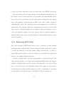
the Java Virtual Machine (JVM) loads classes into memory[14], the static loadLibrary
calls in the VTK code would have two undesirable effects. First, the application would
start slowly because the libraries would be loaded immediately. Worse, if there was
a problem with the native libraries, the application would not start at all. KMC-Vis
is designed to use reflection to load all editors as they are requested to avoid the
problems associated with loading the native libraries as well as decouple individual
editors from the main application.
A common disadvantage of working with JNI libraries is the performance overhead.
Native method calls in Java are significantly slower than non-native calls[13]. VTK
overcomes this problem by allowing the programmer to set up a scene once on the
Java-side, then perform most of the computation within the native implementation.
This coarse-grained architecture minimizes the JNI calls and provides tolerable 3D
performance within Java.
Another advantage of working with VTK is the high-level library support for
44
scientific data. No code within the software created for this project uses primitives
like triangle strips to render surfaces. Rather it uses a data mapping and rendering
pipeline defined by the VTK libraries that is optimized for scientific data. Before
attempting to modify the 3D code within KMC-Vis (or KMC-Mesh) developers would
be well advised to examine the documentation at VTK’s web site[10] because very
few of the OpenGL variety of primitives that may seem familiar are present.
4.2
KMC-Mesh
KMC-Mesh is an extension of the KMC-Vis software. It consists of 16 additional
source code files in two packages. It also relies on code within other KMC-Vis packages. Because of the editor-intensive nature of KMC-Mesh, it requires the finergrained data model observer system alluded to earlier. The following section will
discuss the data model used in KMC-Mesh and also provides a rough guide to a
simple extension.
4.2.1
KMC-Mesh Architecture
The KMC-Mesh software consists of a data model, peers for each object in the data
model, and a set of actions that modify the data. An overview of the data and visualization system is shown in Figure 4.7. KMC-Mesh uses three data model components:
• Model
The model contains at least one (commonly three) Layer object. In addition to
maintaining the list of layers, spacing information and transient view information (e.g. the currently selected layer) is also in the model.
45
Figure 4.7: The KMC-Mesh data model
• Layer
The layer structure contains an array of Element objects that represent all of
the atoms in that layer. It also maintains what type of layer to control x and y
offsets.
• Element
The element structure represents atoms in the simulation. Each atom has a
position on the x, y plane and a type. The type can hold one of three values:
empty, inactive, or active. These values correspond to the type of atom.
Each of these components has a visual peer object within the VTK scene hierarchy.
These peers listen to their counterparts in the data model via the producer-consumer
relationship indicated in Figure 4.7. Any time a data element changes, the visual
peer is updated to reflect the changes to the user.
Currently, the only data contained within the element structures is the state of the
atom. If the editor were updated to support right-click context menus to allow the
editing of individual element properties, the model could easily be updated to include
additional information. In particular, the velocity data in the substrate configuration
file could be added in this way.
46
KMC-Mesh is designed to be independent of KMC-Vis to allow stand-alone execution. This allows users to create, view, and modify mesh files without the overhead
of running KMC-Vis. Of course, the software is also available from within KMC-Vis
during main configuration file generation. While the implementation of this feature
is straightforward when Java is run normally, it is unfortunately complex when the
software is loaded from Java Web Start. The code to correctly configure the class path
and native library directories is in kmcvis.actions.MeshGenTool. This code should be
reviewed when considering any changes to the launch paradigm.
4.3
Deployment
KMC-Vis is available in two forms. The first is a Java Web Start[15] enabled version
of the software that can be launched from the web. The second is a zip file containing
all of the required jars and a batch file. Versions for both Windows and Linux exist
in both cases. The benefit of the web start distribution is that the software will
automatically update the user’s version of the Java Runtime Environment[12] during
launch; unfortunately configuring such a system can be non-trivial. This section will
describe the files used to provide this service in this research.
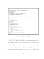
Figure 4.8 is the Java Web Start file that launches the KMC-Vis application from
within a web browser. This text is in a file named “kmcgui.jnlp” and is used simply by
publishing this file and the dependent jars on the web. In order to package java class
files and native libraries they must be placed in signed jars. The process for creating
web start-ready jar files is described in the Java Web Start Developer Guide[16].
Java Web Start-enabled programs are launched using a java virtual machine within
the user’s web browser. If that JVM is not in tact, user’s will need to fall back on
47
<?xml version="1.0" encoding="UTF-8"?>
<jnlp
spec="1.0+"
codebase="http://www.cis.ksu.edu/~clt3955/kmcgui"
href="kmcgui.jnlp">
<information>
<title>Kinetic Monte Carlo -- GUI</title>
<vendor>Charlie Thornton</vendor>
<homepage href="index.html"/>
<description>Kinetic Monte Carlo -- GUI</description>
<description kind="short">A visualization for kmc stuff</description>
<offline-allowed/>
</information>
<security>
<all-permissions/>
</security>
<resources>
<j2se version="1.5+"/>
<jar href="kmcvis.jar"/>
<jar href="vtk.jar"/>
</resources>
<resources os="Windows">
<nativelib href="libs_win32.jar"/>
</resources>
<resources os="Linux">
<nativelib href="libs_linux.jar"/>
</resources>
<application-desc main-class="kmcvis.Run"/>
</jnlp>
Figure 4.8: The JNLP file for KMC-Vis
the zip files provided on the same web page.
There are a few options in “kmcgui.jnlp” that are worth emphasizing. It is a
XML-formatted text file. The codebase option at the top tells the JVM where to
find the jars listed in the resources section; this value must be correct or they will
not be found. Within the security section the “all-permissions” option is listed. This
option allows the application to interact with the user’s hard disk at the expense of a
launch time warning message. In the field: < j2seversion = “1.5+00 > the plus sign
48
indicates that any higher version of the Java VM is acceptable; however if the user has
a lower version, the listed version will be downloaded. The resources section allows us
to specify what jars are downloaded for specific operating systems. Details for these
options and everything else in the file can be found in the developer guide[16].
49
Chapter 5
Results
The most important factor to determine the success of this work was that the users
of the KMC-Vis software would accept and use the software. This software was
introduced to users that were already experienced in managing their data load. They
had software data analysis tools that already provided a means of computing any
of the information accessible through KMC-Vis. In order to measure the success of
KMC-Vis, reviews of the software were solicited from users of SLKMC and KMCVis. The results were very encouraging. Not only did the users believe that the
software was a time-saving tool, but these reviews confirmed that users of the KMCVis software were excited about the project and wanted to see it carried through
to the next level. Section 5.1 will provide details about the user feedback and how
that validates this work. Section 5.2 will discuss a variety of features that could be
included in future versions of the software.
50
5.1
User Acceptance
Three researchers provided evaluations of this work. The entire text of these letters
appears in Appendix C of this document. The first letter (the text of which is in
Figure C.1) was provided by Altaf Karim. Altaf is a graduate research assistant at
the Kansas State University (KSU) physics department. His formal area of research is
condensed matter physics and he is actively using the SLKMC software to examine the
behavior of atomic islands on substrates. The second letter of support (Figure C.2)
was provided by Abdelkader Kara Ph.D. Dr. Kara is a research professor at KSU
specializing in solid state physics. He is also an active researcher in the SLKMC
project. In addition to traditional usage of the KMC-Vis software, he has used
it during a conference presentation to enhance a talk about the SLKMC system.
The third evaluation (Figure C.3) was written by Talat Rahman. Dr. Rahman is
also a professor at KSU; she specializes in atomistic modeling and high performance
supercomputing.
In their reviews, all three users spoke highly of the KMC-Mesh tool for generating
initial mesh configuration files. In support of KMC-Mesh’s visualization and editing
tools, Altaf wrote, “...I had been using another code that generates a crystal structure
but it does not have the ability to create customized ad atom islands on atomic
substrates.” Similarly, Dr. Kara wrote, “...before the building of this software, every
system for KMC simulations had to be built by hand and takes up much more of
the researchers time.” Additionally, Dr. Rahman wrote, “The ability to visualize the
initial positions of the atoms and to change them at will, in an instant, is very handy
and will be very helpful for our future work in the area.” Section 5.2.2 discusses a
variety of features that could be added to the KMC-Mesh software.
51
The analysis phase of KMC-Vis also did quite well in the reviewing process. In
support of the analysis options offered by the software, Altaf wrote the following:
Our SLKMC software generates a pile of large data files. Analysis of
these files is a tedious and time consuming task for a user. This job of
data analysis becomes more complicated when the user has to deal with
files containing information like occurrence frequencies of atomic events.
Indeed, this was a big problem until recently. Now it is being solved to
some extent by making use of the SLKMC User Interface. It offers the
user an essential tool to accumulate and categorize atomic processes on
the basis of their energy barriers.
Dr. Rahman also provided, “We are also very impressed by ability of the software
to analyze the results of the simulations and to quantify the frequencies of various
events, together with visualizations of the processes/events that participate in system
dynamics.” Given the importance of the analysis function of the software, this support
was vital to validate the success of the project.
The non-mesh data generation features, and the simulation execution were not addressed in the reviews. These features provided less functionality within the software
than the mesh generation and data analysis tools. More work needs to be done to
determine the specific needs of users in these area, as well as create an infrastructure
to support software support of items such as remove simulation execution. Details
concerning future features are discussed in the following section.
52
5.2
Future Work
There is plenty of room for improvement in KMC-Vis and KMC-Mesh. This section
will discuss some of the features which ideally should be added to the project in order
to more fully support SLKMC.
5.2.1
Enhancing KMC-Vis
Currently, it is necessary to use the results from a previous simulation to create input
files using KMC-Vis. Ideally, a user should be able to create an entire simulation
model from only a default set of configuration data (stored within the software). The
two input files that can be generated via the user interface are the main configuration
file and the initial mesh configuration. Both of these files are fully editable from the
user interface, but the simulation database and the substrate configuration are not.
Support for managing both of these files could actually be provided through heavy reuse of the existing code base – a database manager would be similar to the statistics
view and a substrate configuration tool would be almost identical to KMC-Mesh.
Once these features were added, users could reasonably expect to create the entire
set of simulation input files.
KMC-Vis supports one of three potential ways to run a SLKMC simulation: loading results from existing files. It should also be possible to run the simulation on a
SLKMC simulation server or simply execute a local SLKMC process and await the results. Unfortunately, this work was done prior to the existence of a simulation server
and such support does not exist. However, even with that limitation it would still be
possible to run simulations in a reduced performance mode using a local process. A
complete version of the software should support all three of these features (unless the
53
local process is made impossible by the new architecture of the SLKMC executable).
The most fertile ground for improvement is in the simulation analysis stage. As
the software evolves both the users and developers find better understanding for how
they can use it more effectively. One key feature that is missing from the analysis
stage is 2D graphing of equations such as MSD of the center of mass. Another is
results filtering to allow only a particular window of the simulation to be available for
analysis. Also, the computer assisted process symmetry detection tool would benefit
from a variety of features including process naming, loading and saving processes to
a file, and statistical sorting tools for the database with and without symmetries.
Analysis features such as these are what makes the software truly useful and require
the most attention.
5.2.2
Enhancing KMC-Mesh
One of the strengths of KMC-Mesh is that it can be generalized to many different
mesh types (rather than just 111), and many different formats. It should be possible
to modify the mesh type at any time during editing. It should also be possible to
plug in different file formats to allow the software to work with other applications
that use a very similar MD-style input file.
Another potential feature is property management for atoms in the mesh. Currently, an atom can have one of three states. Extending KMC-Mesh to also support
substrate configuration files would be a matter of keeping track of velocity vectors in
the x, y, and z directions. Since this functionality would require more user interaction than the mouse clicks currently required, it would be a small matter to generalize
atom parameters and allow the user to customize how they are written out.
54
The visualization window in KMC-Mesh would benefit greatly from a few small
enhancements. The x, y, and z axes are not currently labeled on the 3D axis. This
can create confusion when rotating the view. A related enhancement would be to
include certain preset views for resetting the camera position. Currently users can
return to a (0,0,1) viewing angle using the “Reset View” toolbar option, but it would
also be nice to be able to reset the view to a (1,0,0) camera position.
5.2.3
Extending the Core Simulation Code
A detailed discussion of a distributed SLKMC simulation server is outside the scope of
this document. This section will discuss some of the features that would be desirable
in such a software tool for optimal integration with the user interface software.
Ideally, the computational node responsible for execution of the simulation would
not be present on a user’s workstation. This allows the computationally heavy element
to be executed on specialized hardware and prevent the user from undergoing the
overhead of database files and results storage. It should be possible to submit and
track simulation jobs from within the KMC-Vis software. This requires that the
server provide querying mechanisms for the current state of a user’s simulation.
It should also be possible for the user to control the simulation database used in
a given run. This would allow both open (Self-Learning) and closed databases to be
used. Also, it should be possible to work with and contribute to an ever-growing
database of processes to improve future performance.
Pattern recognition plays an important role both in simulation performance and
in database statistics analysis. These techniques improve the performance of the simulation engine by preventing unnecessary calls to the external function. The current
55
SLKMC implementation applies some rudimentary pattern recognition techniques,
but does not identify all symmetrical processes[7]. As a result, symmetrical processes
leak into the database statistics necessitating the computer-assisted symmetry detection tool discussed in Section 3.1.3. A computational layer that could quickly and
accurately detect symmetrical processes would both improve simulation performance
and completely eliminate a very time-consuming analysis job.
56
Bibliography
[1] Rahman, T., et al, “Atomistic Studies of Thin Film Growth,” Proc. SPIE Annual
Meeting, 5509, 1, (2004)
[2] Ratsch, C., and Venables, J. A., “Nucleation Theory and the Early Stages of
Thin Film Growth” Journal of Vacuum Science and Technology A – Vacuum
Surfaces and Films, 21, 96 (2003)
[3] A. Rahman, “Correlations in the motion of atoms in liquid argon,” Physical
Review 136, A405 (1964)
[4] Wolfram, S., A New Kind of Science, Champaign, IL., Wolfram Media, 2002
[5] Rahman, T. S., Kara, A., Trushin, O., “Cluster Diffusion and Coalescence on
Metal Surfaces: Applications of a Self-Learning Kinetic Monte-Carlo Method,”
MRS Proceedings (2004)
[6] Shim, Y., Amar, J. G., “Synchronous Relaxation Algorithm for Parallel Kinetic
Monte Carlo,” Physical review, B 71, 115436 (2005)
[7] Rahman, Kara, Karim. Private Correspondence (email: [email protected])
57
[8] Wallentine,
V.,
Ramachandran,
A.,
Private
Correspondence
(email:
[email protected])
[9] Gamma, E., et. al., “Design Patterns: Elements of Reusable Object-Oriented
Software,” Addison-Wesley (1997)
[10] “VTK Home Page,” The Visualization Toolkit, Kitware Inc. 14 Apr. 2005
< http://www.vtk.org >.
[11] “Kitware Inc. - Leaders in Visualization Technology,” Kitware Home Page, Kitware Inc. 14 Apr. 2005
< http://www.kitware.com >.
[12] “Download Java 2 Platform, Standard Edition 5.0,” Sun Microsystems, Inc.,
(2005)
< http://java.sun.com/j2se/1.5.0/download.jsp >
[13] Wilson, S., and Kesselman, J., Java Platform Performance: Strategies and Tactics, Sun Microsystems, Inc., (2001)
[14] “ClassLoader (Java 2 Platform SE 5.0),” Sun Microsystems, Inc., 11 Aug. 2004
< http://java.sun.com/j2se/1.5.0/docs/api/java/lang/ClassLoader.html >.
[15] “Java Web Start,” Sun Microsystems, Inc., Oct 5, 2004
< http://java.sun.com/products/javawebstart/developers.html >.
[16] “Java Web Start 1.5.0 Developer Guide,” Sun Microsystems, Inc., Aug. 19, 2004
< http://java.sun.com/j2se/1.5.0/docs/guide/javaws/developersguide/contents.html
>.
58
Appendix A
KMC-Vis Walkthrough
This walkthrough will demonstrate how to use the KMC-Vis software. This document
is appropriate for both the Windows and Linux operating systems.
A.1
Overview
Before we begin, it is important to know exactly what role KMC-Vis plays in the
simulation. A SLKMC simulation requires the following files (the file names shown
are those found in the sample data):
• Main Configuration File (step16m.dt)
A configuration file that specifies global parameters and the names of the other
input files.
• Database (baza c92)
The simulation database consisting of mappings between configurations and
processes.
59
• Substrate Configuration (cu111r.sub)
Configuration file for the substrate used in this simulation.
• Initial Mesh Configuration (clust9i.abk)
An initial mesh configuration.
Using these files, the SLKMC software performs its simulation and dumps out a
number of output files:
• Updated Database (baza c92)
The updated simulation database.
• Database Statistics (clust92.st)
Database process statistics for this simulation run.
• Event Stack (stackc 92)
A complete trace of all simulation processes. This file is huge, not currently
used by KMC-Vis, and not included in the sample data.
• 3D Movie (clust92.m)
A file containing snapshots of the positions of the active atoms.
• Final Mesh (clust92f.abk)
A mesh configuration file suitable to be used as the input for another simulation.
KMC-Vis does not perform any computation for the simulation, rather it assists in
the creation of input files and the analysis of output files.
60
A.2
Getting Started
We will need some sample data for KMC-Vis. A suitable zip file is available on
the Internet at http://www.cis.ksu.edu/~clt3955/research.php. Download and
extract the zip file at the link labeled “sample data.zip”. Remember where this data
is; we will need it later.
We can install and run the software from that same web page. Click the link
labeled “kmcgui.jnlp” under the “Run the Software” heading. This is a Java Web
Start file and will run automatically. Figure A.1 shows the application downloading
necessary files at launch time.
Figure A.1: Running KMC-Vis using Java Web Start
Because KMC-Vis requires access to your hard drive (to read and write SLKMC
files), you will need to grant the application permission to run. Do this by clicking
“yes” in the dialog shown in Figure A.2.
Figure A.2: Grant the application permission to run
61
A.3
Opening a Main Configuration File
You will be greeted by the blank screen shown in Figure A.3. We can now load the
Figure A.3: You will be greeted by a blank screen
sample data we retrieved earlier. Click the File|Open... menu item and browse
to where you extracted the sample data directory. Open the main configuration file
(step16m.dt).
Once the main configuration file is loaded, a variety of data is displayed in the
tabbed panel on the right (shown in Figure A.4). All of the data in the main config-
Figure A.4: The main configuration file editing view
uration file can be edited in the “Input Options” and “Output Options” tabs of this
62
view. Take a moment to flip back and forth between the views by clicking on the
different tabs.
If you change any of the input or output data, a modified main configuration file
can be written using the File|Save As... menu option. In this case, we will be
using the results from a previously run simulation so any changes will not affect the
output (however, modifying any of the input or output filenames make it impossible
for KMC-Vis to load the results).
A.4
Loading Simulation Results
Click the button labeled “Simulate” in the left pane. This will bring up the simulation
execution view shown in Figure A.5. No simulation server is currently available, so
Figure A.5: The simulation execution view
the only option is to load results from files. Click on the button labeled “Start” to
begin reading results data into memory. The status field and progress bar will provide
feedback about the status of data retrieval.
63
A.5
Simulation Analysis
As soon as the database is loaded, the button labeled “Results” in the editor selector
pane will become enabled. Click the “Results” button. The results view shown in
Figure A.6 will be shown in the editor view. From this view we can launch the 3D
Figure A.6: The simulation results and analysis view
results view or analyze the database statistics.
Click the button labeled “3D Results” to bring up another dialog. While the 3D
subsystem prepares the scene a “Rendering” message is displayed, however once the
view is ready to use the message will be replaced by the simulation model. Figure
A.7 shows the progression of the 3D results view. Once the view is ready we can
Figure A.7: 3D results view
manipulate it using the mouse. We can rotate the camera angle by left clicking on
64
the 3D window and dragging the mouse. We can translate the camera position using
the shift key along with a click and drag of the mouse. Finally, it is possible to zoom
in and out using the right mouse button and dragging forward (zoom in) or dragging
backward (zoom out). Take a moment to experiment with the mouse controls. The
zoom and focal point can be reset to default by pressing the ‘R’ key.
Play the simulation moving using the controls at the bottom of the 3D windows.
Playback can be paused at any time using the “Pause” button. When a playback
is paused it is possible to use the “Step Forward” and “Step Back” controls. These
allow you to advance or rewind the simulation one step at a time. The “Stop” button
causes the simulation playback to cease and the current frame to be reset to the first
frame in the simulation movie. Other controls are available on the right side of the
window to control visualization quality and atom size.
Close the 3D results window and return to the top-level results view. Common
database processes (in terms of frequency) are listed in a tree. If you click on an
entry in the tree you will not see a process, rather you will see a configuration that
can result in several processes. If you expand the tree for that configuration and
click on one of its children, you will see arrows added to the previously clear view of
the configuration. These arrows show where atoms within the simulation are moving
during that process. Also, the threshold energy for the process is shown in the “Delta
E” field.
Now that a process has been selected, the “Find Symmetries” button is enabled.
Clicking on this button will produce the dialog shown in Figure A.8; Select one of
the candidate symmetries for the current process and click the “Symmetrical” check
box. For now, don’t worry if the processes are actually symmetrical. Click the “Ok”
button to exit the dialog. The database process list will update to reflect the new
65
Figure A.8: Finding process symmetries
information. If you open up the same process you will see that it now has a child
process. This was the symmetry we just added. The symmetry can be removed by
selecting the parent process, opening the “Find Symmetries” dialog and removing the
check from the candidate process.
66
Appendix B
KMC-Mesh Walkthrough
This walk through will demonstrate how to use the KMC-Mesh software. KMC-Mesh
is a graphical initial mesh configuration generation utility for KMC-Vis. The files
generated by KMC-Mesh are directly useable in SLKMC simulations. This document
is appropriate for both the Windows and Linux operating systems.
B.1
Getting Started
We can install and run KMC-Mesh with a single click. Open a web browser and
go to the web page at http://www.cis.ksu.edu/~clt3955/research.php. Under
the “Run the Software” heading there is a link labeled “kmcmesh.jnlp”. This link
points to a Java Web Start file that will trigger the application launch. Click on the
“kmcmesh.jnlp” link.
Java will automatically download the required libraries to run the application.
Figure B.1 shows the progress indicator for this action.
Because KMC-Mesh requires access to your hard drive, Java Web Start requires
67
Figure B.1: Running KMC-Mesh using Java Web Start
that you permit it to run. Click “yes” in the dialog shown in Figure B.2.
Figure B.2: Grant the application permission to run
B.2
Creating a Mesh
Once KMC-Mesh is open, you will be presented with the (initially blank) split view
interface shown in Figure B.3.
Figure B.3: The initial KMC-Mesh interface
Click File|New.... This will open the “Create Mesh” dialog shown in Figure B.4.
68
This dialog allows you to specify the number of layers, atoms in the x and y directions,
Figure B.4: The mesh creation dialog
and the atom spacing in each direction. The default values will be sufficient for this
example. Click “Ok.” A dialog will display the progress of the operation.
Now that the mesh has been generated, we can experiment with the 3D view and
2D editor. KMC-Mesh allows you to edit a single layer at a time while visualizing
the entire mesh. A yellow box highlights the layer that is currently displayed in the
editor. The 3D view can be manipulated in the same was as the 3D view in KMC-Vis.
Feel free to rotate the view so you can get a better look at the mesh. If thinks get
out of control, you can always press the “Reset View” button on top of the 3D view.
Figure B.5 shows KMC-Mesh after generating the mesh. Notice that in this state, no
Figure B.5: An empty mesh
atoms are active or inactive; they are all set to disabled (or “Empty”). Recall that
69
disabled atoms will not be written to the input file.
We are going to generate two substrate layers and then add some active atoms to
the top layer. To fill an entire layer with inactive (substrate) atoms, click the “Make
Layer Inactive” button in the 2D editor toolbar. Is is a blue circle with an inset
infinity symbol. The result of clicking this button is shown in Figure B.6.
Figure B.6: Filling the bottom layer with inactive atoms
Now use the “Layer Up” 2D editor toolbar button (denoted by an upward pointing
arrow) to shift to the next layer in the z + direction. Notice that the yellow box in
the 3D view is now in the center layer of the mesh. Set all of the atoms in this layer
to inactive using the “Make Layer Inactive” button and shift to the top layer. The
current state of your mesh should be similar to that shown in Figure B.7.
Figure B.7: A complete substrate
Now it is time to add some active atoms to the simulation. Select the “Make Atom
Active” tool (denoted by a circle around a yellow dot) from the toolbar. This tool
70
will allow you to “paint” active atoms onto the layer one atom at a time. Experiment
with this by adding some atoms to the current layer. You may notice that active
atoms are difficult to see underneath the highlighting rectangle in the 3D view. You
can disable the layer highlight using the 3D view toolbar button denoted by blue and
yellow layers. Figure B.8 shows an example of the finished mesh.
Figure B.8: A complete mesh
The 2D editor toolbar also provides tools to zoom in, zoom out, and translate the
view. The translation tool requires you select it, then drag the layer representation
into the desired position. The zoom buttons simply increment or decrement the zoom
each time they are clicked. There are also toolbar buttons to do variants of the tasks
we performed during this walkthough.
B.3
Saving Mesh Data
To write out the mesh we have created, use the File|Save As... menu option. A
file chooser will allow you to specify the location of the file. This file can be used as
an initial mesh configuration file in SLKMC. Any valid initial mesh configuration file
can also be loaded using the File|Open... menu option.
71
Appendix C
GUI Evaluation by Users
This appendix contains the full text of reviews solicited from the users of KMC-Vis
and KMC-Mesh. They support the claims found in Chapter 5 of this document.
72
Dear Prof. Wallentine,
I am writing this letter to express my views about the software, Self Learning
Kinetic Monte Carlo (SLKMC) User Interface, developed by Mr. Charlie Thornton.
This software is equipped with almost all essential tools required for the 3D
visualization of atomistic processes on surfaces.
This nice and beautiful interface also enables a user to create customized
crystal structures or atomic layers having ad atom islands and vacancies.
Prior to Charlies software, I had been using another code that generates a
crystal structure but it does not have the ability to create customized ad
atom islands on atomic substrates.
Our SLKMC software generates a pile of large data files. Analysis of these
files is a tedious and time consuming task for a user. This job of data
analysis becomes more complicated when the user has to deal with files
containing information like occurrence frequencies of atomic events. Indeed,
this was a big problem until recently. Now it is being solved to some extent
by making use of the SLKMC User Interface. It offers the user an essential
tool to accumulate and categorize atomic processes on the basis of their
energy barriers.
In short, Charlie’s work has expanded computational resources and computer
graphics directed at users needs and users interaction with our SLKMC
software.
Sincerely,
Altaf Karim
Figure C.1: Review from Altaf Karim
73
Professor Virgil Wallentine
Computing and Information Sciences Head
Kansas State University
Manhattan KS 66502
Dear Professor Wallentine,
This letter is to report on my experience using the software KMC-GUI developed
by Charlie Thornton as part of his masters thesis. Let me say first that the
final product is very much useful for the researchers involved with kinetic
Monte Carlo (KMC) simulations. In these simulations, the researcher spends
quite sometime in the pre- and post-simulation either preparing the system to
be tackled or analyzing the various products spilled out by the simulation.
Note that in a typical KMC simulation, the evolution of a system, containing
from a few to hundreds of thousands of particles, is evaluated millions to
hundreds of millions of times. The KMC-GUI consists actually of several
components. For the pre-processing of the simulation, the researcher can
automatically generate a system and store it. Note that before the building
of this software, every system for KMC simulations had to be built by hand and
takes up much more of the researchers time. The main advantage of having the
KMC-GUI software comes during the post-processing phase. The researcher may
want to see a movie of the time evolution of the system during the whole or a
part of the simulation. Detailed analysis of correlation functions averages and
distributions of a variety of physical properties have to be performed and the
KMC-GUI allows the research to access this information automatically at a
significant gain in time and accuracy.
Finally, I would like this software grow to satisfy other demands, including
extraction of information as the simulations go.
Sincerely,
Abdelkader Kara
Research Assistant Professor
Department of Physics
Kansas State University
Figure C.2: Review from Abdelkader Kara
74
Professor Virgil Wallentine
Head, Computing and Information Sciences
Kansas State University
Manhattan, Kansas.
May 1, 2005
Dear Professor Wallentine,
I am delighted to write this letter in support of the software KMC-GUI that
Charles Thornton has created as part of his Masters thesis project. The
software reflects a successful collaborative effort between members of two
research groups, one in CIS and the other in Physics. We in Physics are
excited at the final product because it enables us to create initial
configurations for our simulations without the need to create a huge input
file. The ability to visualize the initial positions of the atoms and to
change them at will, in an instant, is very handy and will be very helpful for
our future work in the area. It will also be very useful for external users
of our code, once it is ready to be placed on a dedicated web site. But that
is not all. We are also very impressed by ability of the software to analyze
the results of the simulations and to quantify the frequencies of various
events, together with visualizations of the processes/events that participate
in system dynamics.
In short, I am impressed with the software that Charlie has produced and we
expect to be using it for a long time to come. It has certainly made our work
much easier in terms of both input of data and understanding of the results.
We also expect the software to be very useful in our outreach activities and
in broad dissemination of our results.
Sincerely,
Talat Rahman
University Distinguished Professor
Department of Physics, Kansas State University, Manhattan, KS 66506, USA.
e-mail: [email protected];
|
Phone: +1-785-532-1611
http://www.phys.ksu.edu/~rahman/
|
FAX:
+1-785-532-6806
Figure C.3: Review from Talat Rahmon
75