Download - Josephsmith

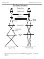
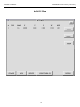
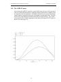
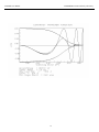
Users Guide
to
NCEMSS
The NCEM program for
the simulation of
HRTEM images
Program written by
Roar Kilaas
Users Guide Written by
Michael A. O’Keefe & Roar Kilaas
National Center for Electron Microscopy
Materials Science Division
Lawrence Berkeley Laboratory
University of California
Berkeley, CA 94720
This work was supported by the U.S. Dept. of Energy under Contract No. DE-AC03-76SF00098
NCEM/MSD Lawrence Berkeley Laborator
NCEMSS User Manual
Section
1. Introduction to the simulation process
1.1
Why simulate images ?
1.2
Describing the transmission electron microscope
1.3
Simplifying the description of the TEM
1.4
Simulating TEM images
2. Introduction to NCEMSS
2.1
The three simulation steps
2.2
NCEMSS files
3. Running NCEMSS
3.1
Getting started
3.2
The SINGLE/LAYERED menu
3.3
The FILE-LIST menu
3.4
The PARAMETER or MAIN or CONTROL menu
3.4.1 Parameters of the PARAMETER menu
3.4.2 Control boxes
3.5
The BASIS menu
3.6
The SYMM-OP menu
3.7
The ATOM-LIST menu
3.8
The BUILD menu
3.9
The ATOM-DISPLAY menu
3.10 The AMPLIT menu
3.11 The CTF plot
3.12 The IMAGE-DISPLAY menu
3.13 The SET-UP menu
3.14 The SET-CONTRAST menu
3.15 The SET-LAYERS menu
Appendix AMultislice Size, PhaseGrating Size, and Maximum G
A.1
Reciprocal-space multislice
A.2
Fourier-transform Multislice
A.3
Real-space multislice
A.4
Storage requirements
Appendix BHOLZ interactions
B.1
Identical slices with only one sub-slice per unit cell repeat distance
B.2
Identical sub-slices with n sub-slices per unit cell repeat distance
B.3
Sub-slices based on atom positions
B.4
Sub-slices based on the three-dimensional potential
B.5
NCEMSS sub-slicing
B.6
Other methods
ii
Page
1
1
1
3
5
7
7
7
11
11
13
15
17
17
21
23
25
27
29
31
33
35
37
39
43
45
47
47
47
49
51
57
57
57
57
57
59
59
NCEM/MSD Lawrence Berkeley Laborator
NCEMSS User Manual
Figures
The SINGLE/LAYERED Menu
The FILE-LIST Menu
The MAIN Menu
The MAIN Menu
The MAIN Menu
The BASIS Menu
The SYMMTRY-OPERATOR Menu
The Atom List Menu
The ATOM-DISPLAY Menu
The AMPLIT Menu
The IMAGE-DISPLAY Menu
The SET-UP Menu
The SET-UP Menu
The Set Contrast Menu
iii
12
14
16
18
20
22
24
26
30
32
36
38
40
42
NCEM/MSD Lawrence Berkeley Laborator
NCEMSS User Manual
NCEMSS - a program for simulation of HRTEM images
1.
Introduction to the simulation process
1.1
Why simulate images ?
Image simulation grew out of an attempt to explain why electron microscope images of
complex oxides sometimes showed black dots in patterns corresponding to the patterns
of heavy metal sites in complex oxides, and yet other images sometimes showed white
dots in the same patterns. This first application was therefore to characterize the experimental images, that is to relate the image character (the patterns of light and dark dots)
to known features in the structure.
Most simulations today are carried out for similar reasons, or even as a means of structure determination. Given a number of possible models for the structure under investigation, images are simulated from these models and compared with experimental
images obtained on a high-resolution electron microscope. In this way, some of the
postulated models can be ruled out until only one remains. If all possible models have
been examined, then the remaining model is the correct one for the structure. For this
process to produce a correct result, the investigator must ensure that all possible models
have been examined, and compared with experimental images over a wide range of
crystal thickness and microscope defocus. It is also a good idea to match simulations
and experimental images for more than one orientation.
Some simulations are done in order to throughly explore one particular image by
“freeze-framing” the imaging process in the computer. In this way, we can obtain information that is not observable experimentally, such as the electron wave amplitude at
the exit surface of the specimen, the magnitude and phase of each component of the image intensity spectrum, or even the amplitude contributed to the intensity spectrum by
each pair of diffracted-beam interferences.
The simulation programs can also be used to study the imaging process itself. By simulating images for imaginary electron microscopes, we can look for ways in which to
improve the performance of present-day instruments, or even find that the performance
of an existing electron microscope can be improved significantly by minor changes in
some instrumental parameter. Alternatively, based on imaging requirements revealed
by test simulations, we can adjust the electron microscope to produce suitable images
of some particular specimen, or even of some particular feature in a particular specimen.
1.2
Describing the transmission electron microscope
In order to simulate an electron microscope image, we need firstly to be able to describe
the electron microscope in such a way that we can model the manner in which it produces the image. As a first step, we can consider the usual geometrical optics depiction
of the transmission electron microscope (TEM).
4
NCEMSS User Manual
NCEM/MSD Lawrence Berkeley Laboratory
5
NCEM/MSD Lawrence Berkeley Laborator
NCEMSS User Manual
Figure 1 shows such a diagram of a TEM operated in two distinct modes, set up for microscopy (a), and for diffraction (b). In microscopy mode we see that the TEM consists
of an electron source producing a beam of electrons that are focused by a condenser lens
onto the specimen; electrons passing through the specimen are focused by the objective
lens to form an image called the first intermediate image (I1); this first intermediate
image forms the “object” for the next lens, the intermediate lens, which produces a magnified image of it called the second intermediate image (I2); in turn, this second intermediate image becomes the “object” for the projector lens; the projector lens forms the
greatly-magnified final image on the viewing screen of the microscope. In microscopy
mode, electrons that emerge from the same point on the specimen exit surface are
brought together at the same point in the final image.
At the focal plane of the objective lens, we see that electrons are brought together that
have left the specimen at different points but at the same angle. The diffraction pattern
that is formed at the focal plane of the objective lens can be viewed on the viewing
screen of the TEM by weakening the intermediate lens to place the microscope in diffraction mode (b).
1.3
Simplifying the description of the TEM
Consideration of the description of the electron microscope in figure 1 shows that the
projector lens and the intermediate lens (or lenses) merely magnify the original image
(I1) formed by the objective lens. For the purposes of image simulation we can reduce
the TEM to three essential components; (1) an electron beam that passes through (2) a
specimen, and then through (3) an objective lens (fig.2).
Our next step in describing the electron microscope for image simulation is to move
from the geometrical optics description of the TEM to a description based on wave optics. In this description of the microscope we examine the amplitude of the electron
wavefield on various planes within the TEM, and attempt to determine how the wavefield at the viewing screen comes to contain an image of our specimen.
By treating the electrons as waves, and considering our simplified electron microscope
(fig.2), we see that there are three planes in the TEM at which we need to be able to
compute the (complex) amplitude of the electron wavefield.
(1)
The image plane:
Working backwards, we start with our desired information, the electron wavefield at the
image plane; this wavefield is derived from the wavefield at the focal plane of the objective lens by applying the effects of the objective aperture and the phase changes introduced by the objective lens.
(2)
The focal plane of the objective lens:
In turn, the electron wavefield at the focal plane of the lens is derived from the wavefield at the exit surface of the specimen by a simple Fourier transformation.
6
NCEMSS User Manual
NCEM/MSD Lawrence Berkeley Laboratory
7
NCEM/MSD Lawrence Berkeley Laborator
NCEMSS User Manual
(3)
The specimen exit surface:
In order to know the exit-surface wavefield, we must know with which physical property of the specimen the wave interacts, and describe that physical property for our particular specimen.
Cowley and Moodie (1957) showed that the interaction of an electron beam with a specimen could be described by the so-called multislice approximation, in which electrons
propagate through the specimen and scatter from the crystal potential; the electron scattering is described by the so-called phase-grating function, a complex function of the
potential, and the electron propagation is computed with a propagation function dependent on the electron wavelength.
1.4
Simulating TEM images
The problem of simulating images thus becomes a problem of computing the electron
wavefields at the three microscope planes. Currently, the best way to produce simulated images is to divide the overall calculation into three parts:
(1) Model the specimen structure to find its potential in the direction of the incident
beam.
(2) Produce the exit-surface wavefield by considering the interaction of the incident
electron wave on the specimen potential.
(3) Compute the image-plane wavefield by imposing the effects of the objective lens on
the specimen exit surface wave.
_________________________________________________________________
Cowley J.M. & Moodie A.F. (1957) The scattering of electrons by atoms and crystals. I. A new
theoretical approach. Acta Cryst. 10, 609.
8
NCEMSS User Manual
NCEM/MSD Lawrence Berkeley Laboratory
9
NCEM/MSD Lawrence Berkeley Laborator
NCEMSS User Manual
2.
Introduction to NCEMSS
2.1
The three simulation steps
Since the simulation problem divides neatly into three parts, NCEMSS treats these three
parts with three sub-programs (1)
PHSGRT - a program to generate the part of the crystal potential that produces
electron scattering; input is from a file containing structural data about the specimen, including unit cell dimensions, symmetries, and atom positions, occupancies, and temperature factors.
(2)
MSLICE - a program to generate the electron wavefield at the specimen exit
surface; it uses PHSGRT data combined with information about the accelerating
voltage of the electron microscope, and the specimen thickness and tilt.
(3)
IMAGE - a program to generate the image intensity at the microscope image
plane; the effects of objective lens phase changes and resolution-limiting aberrations are included via parameters like defocus, spherical aberration, incident
beam convergence, spread-of-focus, and the position and size of the objective
aperture.
Thus PHSGRT considers only the specimen structure, MSLICE treats the interaction of
the specimen with the electron wave, and IMAGE simulates how the wave leaving the
specimen interacts with the lens system of the electron microscope. Once a simulation
has been made, any additional simulation will usually not require a full re-simulation;
any change in microscope parameters will not affect the results of the PHSGRT and
MSLICE programs, and only IMAGE will need to be re-run; any change in microscope
voltage or in specimen thickness or tilt will not affect the results of PHSGRT, but
MSLICE and IMAGE will need to be re-run. Of course, any change in the specimen
structure will require the re-running of all three subprograms.
2.2
NCEMSS files
Supplied files: NCEMSS uses four data files to store supplied information not normally altered by the user:
(1)
spcgrp.dat stores information on all 230 space groups for generation of crystal
symmetry operators as required by the input specimen structures.
(2)
scatt.dat stores information on atomic scattering factors for the first 98 elements.
10
NCEMSS User Manual
NCEM/MSD Lawrence Berkeley Laboratory
11
NCEM/MSD Lawrence Berkeley Laborator
NCEMSS User Manual
(3)
microscopes.dat stores information on the imaging parameters of various highresolution electron microscopes. Note that the user has the option of adding additional microscopes to the table stored in MICROSCOPES.DAT.
(4)
lprint.ps stores a set of Postscript definitions that are used in order to print images to a Postscript Laserprinter.
Generated files: NCEMSS generates and stores various data files in the course of a
simulation. The five data files are:
(1)
name.at stores all the structure and microscope information needed to run the
simulation. This information is derived from user input and the supplied data
files. In particular, the string “name” is a unique name for the structure, input
by the user when creating the structure file.
(2)
name.pout is the result of running the PHSGRT subprogam from the information stored in name.at; it contains the specimen potential in the direction of the
electron beam.
(3)
name.mout is the result of running the MSLICE subprogram using the data in
name.pout with those in name.at; it contains the exit-surface wave at one or
more selected specimen thicknesses.
(4)
name.iout is the result of running the IMAGE subprogram to apply the effects
of the microscope parameters in the name.at file to the exit-surface wave; it contains one or more images ready to be displayed.
(5)
name.aout contains the complex amplitudes of several diffracted beams at oneslice increments in specimen thickness. The beams are specified by the user in
the main menu, and can be plotted as a function of specimenthickness.
In addition, two print files are produced (but rarely printed) just in case additional information about a computation is required by the user. These files are:
(6)
name.p_prnt contains information about the way in which the PHSGRT subprogram processed the name.at data to produce the specimen potential.
(7)
name.m_prnt contains information about the way in which the MSLICE subprogram processed the name.pout data with name.at data to produce the exitsurface wave; that is, it contains information on the multislice computation.
Since NCEMSS images are stored in a file for interactive display, the user has the option of writing any image to the display screen with any selected number of unit cells,
with any selected value of contrast and brightness, and at any selected magnification.
In addition, the user may elect to display (i.e. write to the screen) real-space functions
like the projected crystal potential, the exit-surface electron wavefunction, or a drawing
of the atom positions; in addition, reciprocal-space functions such as the diffraction intensities and the image power spectrum (“optical” diffractogram) may be displayed and
indexed.
12
NCEMSS User Manual
NCEM/MSD Lawrence Berkeley Laboratory
13
NCEM/MSD Lawrence Berkeley Laborator
3.
NCEMSS User Manual
Running NCEMSS
Note on Platform dependency:
NCEMSS was originally written for a terminal emulating tektronix 4014 commands.
The menus were written to the terminal and the images were displayed on a framestore.
The code was executing on a Digital Equipment Corporation microVax II computer under the VMS operating systems. The code has since been ported to other platforms and
will run on DEC VMS and Ultrix workstations and on various flavors of Unix running
X-windows. However, because of the origin of the program, it still an old style layout
dictated by the tektronix terminal. The program uses two windows. One looking like a
graphics window displaying push-button style menus and one window for displaying
graphics output such as images, diffraction patterns and views of unit cells. The program does not have a modern style interface with a menubar and pull down menus.
NCEMSS is run interactively at a graphics screen using a mouse or other pointing device. The graphics screen may be a a workstation console, an X-window terminal or
any computer running as an x-window server. Commands are issued to NCEMSS by
moving a cursor to select an appropriate item from a menu. Sometimes, selecting an
item from a menu will produce another menu with additional options.
Because of constant changes, the menus mentioned in this manual may not always correspond to the current version of the program for a particular platform. The text will be
appropriate for the UNIX version of the program.
3.1
Getting started
If started from an X-terminal, first type setenv DISPLAY <IP address> to set the output to the X-window terminal.
Start NCEMSS by typing ncemss followed by a carriage return:
ncemss (return)
this action will produce the SINGLE/LAYERED menu (page 12), by opening two windows on the workstation screen, one being the menu (control) window, the other the image window.
14
NCEMSS User Manual
NCEM/MSD Lawrence Berkeley Laboratory
The SINGLE/LAYERED Menu
15
NCEM/MSD Lawrence Berkeley Laborator
3.2
NCEMSS User Manual
The SINGLE/LAYERED menu
The first menu encountered by the user on starting to work withNCEMSS consists of
three labeled boxes. Any one of these boxes or buttons can be activated by using the
mouse to move the screen cursor into the area of the screen within the box, and then
pressing the LEFT button on the mouse. At the lower right of the window is the EXIT
box, or button. Selecting this box will cause the program to exit and return to the system
prompt.
The two major boxes allow the user to specify a choice of either a SINGLE STRUCTURE calculation, or a calculation of the images arising from a LAYERED STRUCTURE. A SINGLE STRUCTURE calculation is one where the specimen structure
repeats regularly in thedirection of the electron beam, and is the usual type of image
simulation. A LAYERED STRUCTURE calculation is a simulation in which the specimen structure is built up of a number of different structural layers in the electron beam
direction, so that the computation requires the use of more than one crystal structure
file. Selecting the LAYERED STRUCTURE box produces the SET LAYERS menu
(page 46). Selecting SINGLE STRUCTURE produces the FILE-LIST menu (page 14).
16
NCEMSS User Manual
NCEM/MSD Lawrence Berkeley Laboratory
The FILE-LIST Menu
17
NCEM/MSD Lawrence Berkeley Laborator
3.3
NCEMSS User Manual
The FILE-LIST menu
The FILE-LIST menu lists the user’s structure files on the screen. In addition, there are
four boxes across the top of the menu, and three boxes across the bottom. The four top
boxes control the listing of the structure names; the right hand pair allow the user to
“page” through the list, displaying subsequent pages of structure file names.
The top left boxes can be used to select lists of files from either the user’s PERSONAL
collection of structure files, or from a COMMON collection available to all users on the
system. The files in the COMMON collection can often serve as useful templates for
modification to the user’s needs. On entry to the FILE-LIST menu, the PERSONAL
box is selected automatically. To obtain the COMMON list, move the cursor to the
COMMON box and press the LEFT button on the mouse. To return to your PERSONAL file collection, move the cursor to the PERSONAL box and press the button.
The three boxes at the bottom of the menu are used to proceed from the current menu.
The rightmost box is the RETURN box, and is used to go back to the previous menu.
Note that many menus have this facility, with the RETURN box situated in the bottom
right corner of the menu. The bottom left box is used to notify NCEMSS that the user
wishes to use one of the displayed structure files. Moving the cursor to this USE DISPLAYED FILE box and selecting it by clicking the mouse button removes all the other
boxes, and allows the user to select one of the displayed files by moving the cursor to
the correct filename and clicking the mouse button. Selecting a structure filename
causes NCEMSS to read the file and display its parameters in the PARAMETER menu
(often referred to as the MAIN or CONTROL menu, because it is the one from which
the NCEMSS computation is controlled by the user). The CONTROL menu is shown
on page 16.
The CREATE NEW FILE box is selected when the user desires to input a new structural file. Selecting this box with the cursor causes NCEMSS to ask for a unique name
for the structure. Entry of the name then produces a PARAMETER menu with no parameter values, and a series of prompts from NCEMSS explaining each parameter
needed for input.
HELP: If this is your first use of NCEMSS, it may be helpful to try moving the cursor
to each box in turn, asking for the HELP facility by clicking the CENTER button on the
mouse as each box is reached. The HELP facility is available for every command box
on every menu, and should provide enough information that you will need to consult
this Guide only infrequently.
18
NCEMSS User Manual
NCEM/MSD Lawrence Berkeley Laboratory
The MAIN Menu
19
NCEM/MSD Lawrence Berkeley Laborator
3.4
NCEMSS User Manual
The PARAMETER or MAIN or CONTROL menu
The main CONTROL menu lists a summary of the control parameters for the current
simulation as well as twelve boxes for control of the computation.
When the CREATE NEW FILE option of the FILE-LIST menu (page 14) is selected,
an empty PARAMETER menu (with no control boxes) is presented, and NCEMSS
prompts for parameters. These parameters have the same form as those presented in the
PARAMETER menu when a structure filename is selected from the FILE-LIST menu.
When every parameter has been entered, NCEMSS re-presents the PARAMETER
menu with the control boxes drawn in and available for use.
3.4.1 Parameters of the PARAMETER menu
INPUT FOR: The parameter displayed next to this prompt is a short title for the structure.
SPACE GROUP #: NCEMSS generates symmetry operators for any one of the 230
space groups, when given the number of the space group required (listed in the International Tables for Crystallography). If the space group required is not one listed in the
Tables, a value of zero can be entered.
A, B, C, ALPHA, BETA, GAMMA: These are the unit cell dimensions in Angstrom
units, and the unit cell angles in degrees.
GMAX: The maximum value (in reciprocal Angstrom units) of g to be considered in
the multislice diffraction calculation. This value imposes an “aperture” on the diffracted beams included in the dynamic scattering process. It should be large enough to ensure that all significant beam interactions are included. For light atoms and thin
crystals, values as low as 2.0 are adequate. For structures with heavy atoms and large
crystal thicknesses, values of 3.0 to 4.0 are to be preferred. Note that NCEMSS will
compute phase-grating coefficients out to twice GMAX in order to include dynamical
interactions correctly (Appendix A).
ZONE AXIS: Specimen orientation is selected by specifying the zone axis desired.
Three indices are entered with one space between each.
NO. OF SYMMETRY OPERATORS: If a space group has been selected, the correct
value for this parameter will have been entered by NCEMSS. If a value of zero has
been entered for the SPACE GROUP #, then the correct number of operators must be
entered here.
NO. OF SLICES PER UNIT CELL: For unit cells with large repeat distances in the
beam direction, moderate values of GMAX may allow the Ewald sphere to approach
the so-called pseudo-upper-layer line that the multislice allows at the reciprocal of the
chosen slice thickness. In this case NCEMSS will sub-divide the slice into two or more
subslices. How this is done depends upon the potential setting chosen in the SET-UP
menu (page 40).
20
NCEMSS User Manual
NCEM/MSD Lawrence Berkeley Laboratory
The MAIN Menu
21
NCEM/MSD Lawrence Berkeley Laborator
NCEMSS User Manual
NO. OF ATOMS IN THE BASIS: This value is the number of independent atom positions in the basis or asymmetric unit of the cell. When operated on by the symmetry
operators, the basis generates all the atom positions within the cell.
NO. OF DIFFERENT ATOMS: This value is the number of different types of atoms
in the specimen structure; difference is due to a different Debye-Waller factor or different atomic number.
MICROSCOPE: The type of electron microscope used to generate the imaging parameters. If a type known to NCEMSS is entered, then NCEMSS provide values for CS,
the spherical aberration coefficient of the objective lens (in mm.); DEL, the halfwidth
of a Gaussian spread of focus due to chromatic aberration (in Angstrom units); TH., the
semi-angle of incident beam convergence (in milliradian). If the type of microscope is
unknown to NCEMSS, the above values must be entered seperately (or the data file MICROSCOPES.DAT may be edited to include an appropriate microscope type).
FOIL THICKNESS: The thickness of the specimen foil may be entered as one single
number representing the thickness in Angstrom units, or as a series of thicknesses represented by the upper and lower bounds and a thickness step; e.g. 100(50)250 will cause
NCEMSS to store the exit wavefield at specimen thicknesses of 100Å to 250Å in steps
of 50Å (a total of four thicknesses).
AMPLIT. OUTPUT FOR PLOTTING: A number of diffracted beams may be selected for plotting of their intensity and phase variation as a function of specimen thickness.
If YES is answered to the NCEMSS prompt, the number of beams and their indices may
be entered.
VOLT.: The electron microscope accelerating voltage in kilovolts.
CENT. OF LAUE CIRCLE: Specimen tilt is specified by entering the center of the
Laue circle in units of the h and k indices of the projected two-dimensional reciprocalspace unit cell.
DEFOCUS: The defocus of the objective lens is entered in Ångstrom units with a negative value representing underfocus (weakening of the lens current). As for the FOIL
THICKNESS parameter, a single value of defocus may be entered, or a range specified
by the upper and lower bounds and the interval; -300(-200)-1100 means defocus values
of -300Å, -500Å, -700Å, -900Å and -1100Å.
APERTURE RADIUS: The radius of the objective aperture is specified in reciprocal
Ångstrom units.
CENT. OF OBJ. APRT.: The center of the objective aperture is defined in units of the
h and k indices of the two-dimensional reciprocal-space unit cell, as for the Laue circle
center.
CENT. OF OPTIC AXIS: The center of the optic axis of the electron microscope is
specified in terms of the h and k indices of the two-dimensional reciprocal-space unit
cell, just as for the Laue circle center and the aperture center.
22
NCEMSS User Manual
NCEM/MSD Lawrence Berkeley Laboratory
The MAIN Menu
23
NCEM/MSD Lawrence Berkeley Laborator
NCEMSS User Manual
3.4.2 Control boxes
CHANGE: When the CHANGE box is activated by clicking the mouse with the cursor
within the CHANGE box boundaries, any parameter value may be changed simply by
moving the cursor to the parameter position, clicking the mouse and entering the new
value from the keyboard in response to the NCEMSS prompt. To leave CHANGE
mode, deactivate the CHANGE box by clicking the mouse with the cursor once again
positioned over the CHANGE box.
RUN: Activating the RUN box will cause NCEMSS to run an image simulation for the
current values of the parameters shown in the PARAMETER menu. NCEMSS will automatically run the least required computation, starting with the PHSGRT program only
if a structure parameter has been changed since the last run of this data, and starting with
the IMAGE program if the only change has been in the electron microscope imaging
parameters.
SHOW BASIS: This box will cause NCEMSS to display the BASIS menu, a list of the
atom positions making up the basis (page 22).
SHOW ATOMS: this box will cause NCEMSS to display the ATOM-LIST menu, a
list of all the atom positions in the unit cell (page 26).
PHSGRT: Activating the PHSGRT control box will run the PHSGRT sub-program for
the current parameter values.
MSLICE: Activating the MSLICE control box will run the MSLICE sub-program for
the current parameter values.
IMAGE: Activating the IMAGE control box will run the IMAGE sub-program for the
current parameter values.
AMPLIT: Activating the AMPLIT control box will open up a plotting window (page
34), and ask the user which of the stored diffracted beam amplitudes to plot (assuming
that some diffracted beams were stored by specifying their indices before the MSLICE
was run).
DISPLAY: This control box is used to activate the IMAGE-DISPLAY menu (page 38)
for writing images to the display screen.
VIEW FILE: Activating this control box causes NCEMSS to ask which print file to
display, then to display it.
CTF: Activating this control box produces a linear-image Contrast Transfer Function
under the imaging conditions specified by the current parameter values (page 36).
RETURN: Return to previous FILE-LIST menu.
24
NCEMSS User Manual
NCEM/MSD Lawrence Berkeley Laboratory
he BASIS Menu
25
NCEM/MSD Lawrence Berkeley Laborator
3.5
NCEMSS User Manual
The BASIS menu
The BASIS menu shows a list of the atom positions making up the basis; when operated
upon by the symmetry operators, the basisyields the full set of unit cell atom positions.
The BASIS menu displays the atom positions, showing the chemical symbol (NAME)
for each atom, its fractional coordinates (X,Y,Z), the Debye-Waller factor, and the site
occupancy. Subsequent pages of long lists can be viewed with the three right-hand control boxes.
CHANGE: The value of any parameter can be changed by activating the CHANGE
box, then moving the cursor to the parameter position, clicking the mouse and entering
the replacement value.
ADD: Additional atom positions may be added by activating the ADD box and entering parameter values in response to prompts.
DELETE: Activating the DELETE box, then moving the cursor to the appropriate line,
will delete the line.
SHOW SYMM. OP: A list of the symmetry operators may be obtained by activating
this control box in order to bring up the SYMM-OP menu (page 24).
RETURN: Return to previous MAIN menu.
26
NCEMSS User Manual
NCEM/MSD Lawrence Berkeley Laboratory
The SYMMTRY-OPERATOR Menu
27
NCEM/MSD Lawrence Berkeley Laborator
3.6
NCEMSS User Manual
The SYMM-OP menu
The SYMM-OP menu shows a list of the symmetry operators generated by the chosen
space group (or input by the user when a space group number of zero is entered in the
MAIN menu - see page 20). The right-hand control boxes are used to page through long
lists of symmetry operators.
CHANGE: Any operator may be replaced by activating the CHANGE box, clicking
the mouse over the appropriate line, and entering the new operator.
ADD SYMMOP: Activating this control box enables the user to add a new operator to
the list.
DELETE SYMMOP: Activating this box, then placing the cursor over any operator
and clicking the mouse, will delete that operator.
RETURN: Return to previous BASIS menu.
28
NCEMSS User Manual
NCEM/MSD Lawrence Berkeley Laboratory
The Atom List Menu
29
NCEM/MSD Lawrence Berkeley Laborator
3.7
NCEMSS User Manual
The ATOM-LIST menu
The ATOM-LIST menu shows a list of the atom positions making up the unit cell. The
list displays the atom positions one per line, showing the chemical symbol (NAME) for
each atom, its fractional coordinates (X,Y,Z), the Debye-Waller factor (DW), and the
site occupancy (OCC). Subsequent pages of long lists of atom position parameters can
be viewed with the three right-hand control boxes.
BUILD CELL (not implemented on Unix Versions): Activating the BUILD control
box brings up the BUILD menu (page 28) with the facility of generating defect cells.
DISPLAY: Activating this control box brings up the ATOM-DISPLAY menu (page
30), for the purpose of drawing an atom model of the current structure (page 32).
RETURN: Return to previous MAIN menu.
30
NCEMSS User Manual
NCEM/MSD Lawrence Berkeley Laboratory
31
NCEM/MSD Lawrence Berkeley Laborator
3.8
NCEMSS User Manual
The BUILD menu
The BUILD menu is used to create defect cells visually with the aid of the cursor. The
menu has a right-hand column of control buttons, activated in the usual way.
INCR_X: This button is used to increment the unit cell in the x direction. The INCR_Y
button does the same in the y direction. When the INCR_X button is activated,
NCEMSS will ask for the additional number of repeats to be input from the keyboard.
Note that the total length of the new cell in the x-direction will be the original length
plus the number of increments specified.
DISPLAY: This control box is used to display the current defect cell, and should be
used on entering the menu, and after each change made to the defect cell.
INSERT: To insert an atom, activate this box and move the cursor to the required position. Note the changes in the fractional coordinates displayed in the bottom line of the
menu as the cursor is moved. NCEMSS will prompt for parameter values.
REMOVE: To remove an atom, activate this box and move the cursor to the appropriate atom, then click the mouse.
MOVE: To move an atom, activate this box, move the cursor to an atom position, click
the mouse, move the mouse to the new position (note the fractional coordinates), and
click again.
CHANGE: To change the atomic number of an atom, activate this box, and click the
mouse at the atom position.
RETURN: Return to previous ATOM-LIST menu.
32
NCEMSS User Manual
NCEM/MSD Lawrence Berkeley Laboratory
The ATOM-DISPLAY Menu
33
NCEM/MSD Lawrence Berkeley Laborator
3.9
NCEMSS User Manual
The ATOM-DISPLAY menu
When DISPLAY is selected in the ATOM-LIST menu (page 26), most of the control
buttons are replaced to produce the ATOM-DISPLAY menu. The ATOM-DISPLAY
menu has only four control boxes.
UNIT CELL: Activating this box splits it in two. Selecting either option causes
NCEMSS to ask for the viewing direction indices to be input from the keyboard;
NCEMSS then draws the unit cell, either with or without perspective (page 32).
NEW UNIT CELL: As for UNIT CELL, but for drawing any new unit cell produced
with the BUILD menu (page 28).
3-D ATOM DISPLAY: This control box initiates a three-dimensional atom drawing
routine based on a routine written by W.O. Saxton. It can be used to produce publication-quality atom model drawings with a wide range of different lighting conditions.
This procedure is not implemented on most versions of NCEMSS, specifically all unix
version
RETURN: Return to previous ATOM-LIST menu.
34
NCEMSS User Manual
NCEM/MSD Lawrence Berkeley Laboratory
The AMPLIT Menu
35
NCEM/MSD Lawrence Berkeley Laborator
NCEMSS User Manual
3.10 The AMPLIT menu
On activating the AMPLIT control box on the MAIN menu, the user will be presented
with a list of the diffracted beams for which the complex amplitudes are currently stored
as a function of specimen thickness. NCEMSS will ask the user to select which beams
to plot, whether to superimpose the plots, and whether to include phase plots. The plots
will be drawn with thickness horizontal and marked in Angstrom units. The various
curves can be marked with the appropriate beam indices by using the TEXT option of
the SET-UP menu (page 38).
36
NCEMSS User Manual
NCEM/MSD Lawrence Berkeley Laboratory
37
NCEM/MSD Lawrence Berkeley Laborator
NCEMSS User Manual
3.11 The CTF plot
The result of activating the CTF control button on the MAIN menu is a plot of the linear-image Contrast Transfer Function. This function is first plotted as the undamped
sine part of the complex phase change due to the objective lens spherical aberration and
defocus. The damping curves due to the effects of spatial and temporal coherence (incident beam convergence and spread of defocus) are plotted next, then finally the result
of imposing the damping on the sine curve. Remember that this curve is only useful for
estimating the linear contribution to the image of the diffracted beams exiting a thin
crystal (one in which they have suffered only essentially kinematic scattering).
38
NCEMSS User Manual
NCEM/MSD Lawrence Berkeley Laboratory
The IMAGE-DISPLAY Menu
39
NCEM/MSD Lawrence Berkeley Laborator
NCEMSS User Manual
3.12 The IMAGE-DISPLAY menu
When DISPLAY is selected in the MAIN or CONTROL menu (page 16), NCEMSS
brings up the IMAGE-DISPLAY menu. This menu consists of 21 control buttons. The
top three are used to select various options that remain until reset. The left-hand column
is used to select the function to be displayed. Other control boxes select the actions to
be taken.
WORKSTATION/LASERPRINTER: These two boxes are mutually exclusive and
are used to select the output device for the image display.
CHANGE DEFAULTS AND RUN MISC. FUNCTIONS: This control is used to
bring up the SET-UP menu (page 40) where various imaging options and defaults may
be set.
POTENTIAL: Selecting this input produces a display of the unit cell potential projected in the incident electron beam direction.
EXIT-WF: The electron wavefield at the crystal exit surface may be displayed by selecting this input function.
DIFFR.PAT.: Selects the diffraction pattern for display.
IMAGE: Selects the current image for display.
HISTOGR: Produces a histogram of the intensity values in the function selected from
column one.
HIST.EQ.: Stretches the image contrast by performing a histogram equalization operation before display.
ADJ.CNT: Brings up the SET-CONTRAST menu (page 44) for selection of contrast
parameters before display.
FFT: Performs a fast Fourier transform on the selected function and squares the result
before display. (Performed on the image, FFT produces the image power spectrum or
“optical diffractogram”).
#UN.CLS: Enables input of the number of unit cells desired in the displayed image.
ZOOM: Asks for a factor to use in magnification the image.
DISPLAY: Directs the output to the display device.
EXECUTE: Takes the selected function, applies the selected operations, and outputs
the picture.
CANCEL: Cancels the selected options, usually because one was selected by mistake.
40
NCEMSS User Manual
NCEM/MSD Lawrence Berkeley Laboratory
The SET-UP Menu
41
NCEM/MSD Lawrence Berkeley Laborator
NCEMSS User Manual
3.13 The SET-UP menu
Opting to change the various defaults by selecting the CHANGE box in the IMAGEDISPLAY menu (page 38), brings up the SET-UP menu. This menu is used to change
the default settings of some “hard” parameters, and to manipulate the image display.
The nine two-way switches on the left of the menu are normally set to default to the lefthand setting.
SET ERASE<>NOERASE: When ERASE is set, the display screen will be erased before each new image is displayed (except see MONTAGE).
SET NOMONTAGE<>MONTAGE: When NOMONTAGE is set, only one image
will be displayed for each activation of the EXECUTE command from the IMAGEDISPLAY menu (page 38). When MONTAGE is set, then a full through-thickness and/
or through-focus series of images will be displayed at one EXECUTE command (assuming the calculation was carried out for such a series by setting the appropriate parameter values in the PARAMETER menu (page 16)). Note that a MONTAGE will
erase the screen before display, regardless of the ERASE setting.
SET NOREQ-POS<>REQ-POS: When NOREQ_POS is set, individual images will
be written to the center of the display screen (assuming that NOMONTAGE is set).
When REQ_POS is set, the user will be prompted for the coordinates at which the image is to be displayed.
NOMONT-SPACE<>MONTAGE-SPACE: is used to set the desired spacing between the montaged images.
INT.AUTO-SCALE<>INT.ABS-SCALE: To see the most detail in any image, set
INT.AUTO-SCALE to display the image with its minimum set to black and its maximum to white. To intercompare images, it is better to use INT.ABS-SCALE to choose
the same absolute scale for all the images.
CTF-AUTOSCALE<>CTF-ABS.SCALE: Can be used to scale a CTF plot (page
36) by fixing the maximum g value considered. In AUTOSCALE mode the CTF is
drawn to where it approaches zero.
PG-REC SP<>PG-REAL SP: determines whether or not the calculation is done in reciprocal space or in real space. This switch should be set to reciprocal space since the
real space calculation is not debugged yet.
APERTURE<>NO-APERTURE: determines whether or not the current objective aperture radius is drawn on a displayed diffraction pattern.
TITLES<>NO TITLES: determines whether titles are written under each displayed
image. Notice that MONTAGE will supress titles, but a title for the montaged series
may be added using WRITE TEXT.
2D-POT.SLICE<>3D-POT.SLICE: When the number of slices per unit cell exceeds
one in the MAIN menu (page 16), NCEMSS will sub-slice the unit cell in one of two
ways. When 2D-POT is set, the total potential within the cell will be projected, and a
portion assigned to each sub-slice. A more-accurate method is to approximate the upper-layer zones by sub-slicing a three-dimensional potential into the required number
of sub-slices. In this way the variation of the specimen structure in the electron beam
direction is included in the simulation. Of course, it takes longer in 3-D).
SET MIN. INTENSITY (LENS): sets the minimum diffracted beam intensity that will
be considered to pass through the objective lens; this minimum can be set to exclude
very low intensity beams from large defect unit cells, and so speed up the image calculation.
SET MIN.INT.TO DISPLAY(FFT): determines down to what intensity diffracted
beams will be drawn in a diffraction pattern display.
42
NCEMSS User Manual
NCEM/MSD Lawrence Berkeley Laboratory
he SET-UP Menu
43
NCEM/MSD Lawrence Berkeley Laborator
NCEMSS User Manual
SET CAMERA LENGTH: is used to adjust the magnification of the diffraction pattern display. The value is input in mm., and has a default setting of 520mm.
INDEX DIFFR.PT.: is used to index a diffraction pattern. On moving the cursor to
the selected diffraction spot and clicking the mouse, the indices are written next to the
spot.
CHANGE CENTER OF DIFFR.PT.: The center of the displayed diffraction pattern
can be changed by selecting this command and using the mouse to click on the desired
position in the image display window.
READ THE CURSOR POSITION: reads the cursor position within an image.
ERASE THE DISPLAY: does just that.
WRITE TEXT ON THE DISPLAY: is used to write text at the cursor position.
STORE PARTS OF THE DISPLAY: after selecting this command, mark the corners
of an area of the display window (image) to be stored and the image will be saved in a
file. The user is prompted for a name and the program will automatically add the extension .at
DISPLAY STORED IMAGE: use this command to displayed a stored image of the
type <name>.at created by the previous command.
PRINT STORED IMAGE FILE: sends the content of the file <name>.at to a connected laserprinter. The program creates a file “laserprinter.ps” and uses the command “lpr
laserprinter.ps” to send the file to the printer. It is up to the user to set up the appropriate
redirection of the output to a valid printer.
PRINT THE SCREEN: sends the content of the image window to a connected laserprinter. It otherwise works identical to the command above.
LIST STORED IMAGE-FILES: sends the command “ls *.im” to the operating system. The output list of stored image files is displayed in the terminal session window.
SET CONTRAST FOR LASERWRITER: allows the user to change the values of
brightness (normally 0.5) and contrast (normally 1.0) of the printed image
SET DIV.ANGLE FOR DP: use this to change the size of the displayed diffraction
spots in case the size is not optimal for viewing.
IMAGE ONLY<>OVERLAY ATOMS: controls whether atom positions are overlayed on the image or not.
AUTOSCALE-FIXED: use this to either let the computer choose black and white levels automatically or to use fixed values input by the user.
DISPLAY<>PRINT: in the display position, anything “DISPLAYED” goes to the image window. In the PRINT position, the actual numeric data is sent to a file in a format
that depends on the setting of the switch ascii/binary below.
REL PHASE <> PHASE: determines if the phases reported for diffracted beams include the phasechange due to the mean inner potential of the crystal
ASCII FILE<>BINARY FILE: determines if the numeric output data for an image,
projected potential or complex wavefunction is in ascii or binary.
OUT->PRINTER<>OUT->FILE: normally when you reroute the output to the printer, the program executes the command “lpr laserprinter.ps”. Selecting OUT->FILE will
create a named postscript file that can be saved and printed at any time later.
NORM.MONT<>CUSTOM: allows extra control on the layout of montaged images.
44
NCEMSS User Manual
NCEM/MSD Lawrence Berkeley Laboratory
The Set Contrast Menu
45
NCEM/MSD Lawrence Berkeley Laborator
NCEMSS User Manual
3.14 The SET-CONTRAST menu
When the ADJ.CNT box of the IMAGE-DISPLAY menu (page 38) is activated, it
brings up the SET-CONTRAST menu. This menu displays the current contrast and
brightness settings graphically. The straight line shows the mapping of the image intensity values (horizontal axis) into the displayed output intensity values (vertical axis).
For a one-to-one mapping, the values of contrast (vertical bar-graph) and brightness
(horizontal bar-graph) should be 1.0 and 0.5 respectively.
To increase (or decrease) the contrast used to display the image, tap the mouse with the
cursor positioned over the UP (or DOWN) boxes underneath the vertical bar-graph.
The contrast-transfer graph will pivot about its mid-point as the contrast is changed,
providing a plot of how input grey levels are mapped into output greyscale levels. Note
that a contrast value of less than zero will produce a negative image.
To increase (or decrease) the image brightness, use the INCR. and DECR. boxes to
move the mid-point of the contrast-transfer graph to the left or right.
The contrast-transfer curve may be set directly, by activating the SET BLACK-WHITE
box, then clicking the mouse after positioning the cursor at one end-point of the desired
line, then clicking at the other endpoint. These end-points need not be exactly on the
lines forming the box enclosing the contrast-transfer graph.
46
NCEMSS User Manual
NCEM/MSD Lawrence Berkeley Laboratory
47
NCEM/MSD Lawrence Berkeley Laborator
NCEMSS User Manual
3.15 The SET-LAYERS menu
If the LAYERED STRUCTURE option is selected from the SINGLE/LAYERED
menu (page 12), then the SET-LAYERS menu appears. This menu can be used to “construct” a specimen consisting of multiple layers of different single structures.
DEF LAY: To include a structure in the phase-grating sequence thatwill comprise the
final layered structure, use the DEF LAY box and enter the name of the structure as it
appears in the FILE-LIST menu (p.14). Up to six different structures may be used to
make up the layered structure. Note that a PHSGRT calculation (p.21) must be carried
out for any structure before it can be included in a layered calculation. Also note that,
as well as existing, all the phase-gratings used to build a layered structure must be the
same shape and size; i.e. each phase-grating must have the same values for the projected
(two-dimensional) cell axes and cell angle, and also be computed out to the same scattering parameter, GMAX.
DEL LAY: This box is used to remove a previously-defined layer name from consideration.
DEPOSIT: The layered structure can be built up by depositing layers of any member
structure that was defined earlier using DEF LAY. Each deposition is made by clicking
on the DEPOSIT box, then on the appropriate LAYER symbol, then entering the layer
thickness desired. The final structure is built from the top down; i.e. each subsequent
layer is deposited onto the bottom of any existing sequence. A graphical repesentation
of the structure appears on the left of the menu, and the phase-grating sequence is also
listed.
INSERT: In addition to depositing a specified thickness of a chosen layer, it is possible
to insert a specified thickness at any chosen thickness of the final structure. Clicking
on this button, followed by the appropriate LAYER symbol, causes NCEMSS to ask for
a layer thickness to be inserted, and the structure thickness at which to insert it.
REPEAT: This button is used to repeat a defined sequence a chosen number of times
in order to build up a periodic layer structure.
RESET: This button zeros everything in preparation for another try.
REMOVE: The phase-grating sequence can be operated on directly to remove single
slices, one at a time, by activating this button and clicking on the offending phase-grating in the sequence.
48
NCEMSS User Manual
NCEM/MSD Lawrence Berkeley Laboratory
49
NCEM/MSD Lawrence Berkeley Laborator
NCEMSS User Manual
Appendix AMultislice Size, PhaseGrating Size, and Maximum G
The “size” of a multislice calculation is defined conveniently by the size of the
largest array (the Q(k) or q(x) array). For an array size of 2nx2m, the multislice is said
to be a “parameter n+m” multislice; thus a parameter-16 multislice will have a Q(k) array size of 256x256, (or 512x128, or 1024x64, or 2048x32, or 4096x16, depending
upon the shape of the unit cell used in the computation). This size parameter must apply
to all multislice programs, regardless of which of the three current algorithms (reciprocal-space, Fourier-transform, or real-space) is employed by the program.
A.1
Reciprocal-space multislice
As introduced by Goodman and Moodie (1974), the basic recursive form of the multislice description of dynamical diffraction can be written as
Ψn+1(k) = [Ψn(k) • Pn+1(k)] * Qn+1(k)
(A1)
That is, Ψn+1(k), the wave function (given in reciprocal space) at the exit surface of the
(n+1)th slice, is obtained by multiplying the wave function at the exit surface of the nth
slice by Pn+1(k), the propagator for the (n+1)th slice, followed by the convolution of this
result by Qn+1(k), the phase-grating function (given in reciprocal space) for the (n+1)th
slice.
In multislice computer programs that use the above reciprocal-space formulation, the three functions, Ψ(k), P(k), and Q(k) are represented by two-dimensional arrays containing terms with indices that can be regarded as those of the diffracted beams
within the diffracting specimen. In order to impose no extra symmetry on the computation, a “circular aperture” is usually placed on the terms in the arrays, so that terms
beyond a certain distance in reciprocal space are set to zero. Note that the Q(k) array
must extend out to twice as far in reciprocal space as the Ψ(k) and P(k) arrays in order
to correctly include all physical scatterings to each diffracted beam. Figure A1 shows
how this doubled phase-grating requirement arises because Q(k) is a “probability map”
of terms that determine how much of each diffracted beam is to be scattered through the
angle corresponding to the term. Thus, in order to compute the scattering of diffracted
beams out to k = ±(h,k), the Ψ(k) and P(k) must be (2h+1)x(2k+1) in size, and Q(k)
must be (4h+1)x(4k+1). For example, the SHRLI80 programs used a 128x128 array for
Q(k), making SHRLI80 a parameter-14 multislice and giving a maximum (h,k) value
of (31,31); this limits the number of diffracted beams to less than 4096, adequate for
most perfect-crystal computations, but too small for simulation of many defect structures (O’Keefe et al, 1978).
A.2
Fourier-transform Multislice
For larger arrays (and thus larger numbers of diffracted beams), it is faster to
compute the multislice by recasting (A1) into a form where the convolution is replaced
by two Fourier transforms and a multiply operation, as was done by early users of multislice in the Melbourne group. Then
50
NCEMSS User Manual
NCEM/MSD Lawrence Berkeley Laboratory
(a)
n- 1
Q n-1( k)
k = 2
k
F ( k' )
k' = 2
2, 0
0
1
1
2
0
1
1, 1
1
0, 2
2
Q n( k)
2, 4
1, 3
F ( k' ) Q( k- k' ) =
2, 4
2, 1
2, 3
1, 3
1, 0
1, 2
2, 2
0, 2
0, 1
0, 1
1, 1
1, 1
1, 2
1, 0
0, 0
2, 0
2, 3
2, 1
1, 1
2, 2
(b)
2
1
0
1
2
*
=
4
3
2
1
0
1
2
3
4
2, 0 2, 1 2, 2 2, 3 2, 4
1, 1 1, 0 1, 1 1, 2 1, 3
0, 2 0, 1 0, 0 0, 1 0, 2
F( k')
Q( k- k')
1, 3 1, 2 1, 1 1, 0 1, 1
2, 4 2, 3 2, 2 2, 1 2, 0
∑F(k')Q(k-k') =
2
(k)
1
0
1
2
( k)
k'
Fig. A1. Convolution description of multiple scattering. In order to include all scattering contributions to
the dynamic electron wavefield Ψ(k), the phase-grating coefficients Q(k) must extend out twice as far in reciprocal space as do the coefficients of the wavefield. For the five depicted diffracted beams Ψ(k), (where
|k|= -2,-1,0,1,2), the convolution requires nine phase-grating coefficients Q(k), (where |k|= -4 to 4).
(a) sketch of the contributions to the five diffracted beam directions; note that (e.g.) the contribution of the
incoming Ψ(2) beam to the outgoing Ψ(-2) beam requires the presence of the Q(-4) phase-grating coefficient.
(b) Delta-function representation of the scattering process, showing each F(k’).Q(k-k’) term contributing to
the outgoing Ψ(k), |k| = -2 to 2. Here the incoming function F(k) is equal to the product Ψ(k).P(k) in equation (A1). Note the presence of the Q(±3) and Q(±4) coefficients in the table of interactions; except for Ψ(0),
every outgoing Ψ(k) contains a contribution from these outer coefficients, and would be in error without
them.
51
NCEM/MSD Lawrence Berkeley Laborator
NCEMSS User Manual
Ψn+1(k) = F [F -1[Ψn(k) • Pn+1(k)] • qn+1(x)
(A2)
Here the F represents the Fourier transform operation, and q(x) is the real-space form
of Q(k), i.e. the (inverse) Fourier transform of Q(k). Experience with the SHRLI programs has produced the not-surprising result that, in order to obtain the same results
with (A2) as with (A1), q(x) must be formed from a Q(k) that extends twice as far in
reciprocal space as do Ψ(k) and P(k).
Note that, as well as correctly describing the physics of the scattering process
by ensuring that all contributions from all the diffracted beams leaving the previous
slice to each diffracted beam from the current slice are included, the doubled phasegrating also neatly eliminates the possibility of any “aliasing” arising from the necessary sampling of the real-space functions. Unfortunately, in their description of the FFT
multislice, Ishizuka and Uyeda (1977) stated that the number of diffracted beams must
be no less than the number of phase-grating coefficients; under their condition, the effects of aliasing will produce incorrect scattering results if array sizes are not made large
enough to produce essentially zero electron amplitude over the outer five-nineths of the
phase-grating and wave-amplitude arrays. This confusion appears to have arisen when
the concept of FFT multislice was introduced to the Kyoto group by a visiting researcher familiar with its use in the Physics Department of Melbourne University. At Melbourne, it had been found that aliasing occurred when the convolution step of the
reciprocal-space multislice (equation A1) was replaced by a forward/inverse Fourier
transform sequence. This aliasing boosted the amplitudes of the outer beams in the calculation until “knock off” parameters were introduced to set the outer beam amplitudes
to zero after each slice. However, even after this procedure eliminated the aliasing effect, results from the FFT multislice did not exactly match ones from the “standard” reciprocal-space formulation (O’Keefe, 1972). For this reason, the SHRLI80 programs
(O’Keefe et al, 1978) continued to use the (slower) reciprocal-space form of the multislice. Experiments with various scattering algorithms (Self et al, 1983) led to the testing
of different ways of avoiding aliasing in FFT multislice. It was realized that one such
method was by choosing a q(x) formed from Q(k) terms that extended only 2/3 of the
way to the array edges, provided that only the same number of diffracted beams was
used in Y(k), with the outer 5/9 of the diffracted beam array reset to zero after every
slice. A better method was to ensure that q(x) was formed from a Q(k) that extended
out to twice the scattering angle as Ψ(k), and to reset the outer 3/4 diffracted beams to
zero after each slice. This latter method conforms to the physics of the scattering process (fig.A1), and proved to yield the same results as the reciprocal-space multislice. A
multislice program using this method was incorporated into the SHRLI81 suite, and this
method is used in the NCEMSS multislice program (O’Keefe and Kilaas, 1988).
A.3
Real-space multislice
A third method of computing the multislice is to carry out the calculation completely in real space; this is an alternative to computing in reciprocal-space (as in equation A1), or in both real and reciprocal-space (as in equation A2). Fourier
transformation of (A1) gives
52
NCEMSS User Manual
NCEM/MSD Lawrence Berkeley Laboratory
53
NCEM/MSD Lawrence Berkeley Laborator
NCEMSS User Manual
ψn+1(x) = [ ψn(x) * pn+1(x) ] • qn+1(x)
(A3)
In this formulation the real-space wave function yn(x) is convolved by a realspace propagator pn+1(x) and the result multiplied by the real-space phase-grating. Van
Dyck (1983) has developed this method and shown that the convolution step need not
be carried out with the full 2nx2m p(x) array, but only with a such smaller array (since
p(x) is sharply peaked in the forward direction for high energy scattering). Since the
modified p(x) array is so much smaller, the computation time should take less time than
either of the reciprocal-space multislice (A1) or the FFT multislice (A2); however, tests
(e.g. Kilaas and Gronsky, 1983) have shown that the original formulation of the method
required more beams and smaller slices to achieve the same precision as either the reciprocal-space multislice or the FFT multislice, resulting in a longer time to produce
the wavefield at the same total specimen thickness. Van Dyck and Coene (1984) have
since proposed a modified implementation of the real-space multislice into a workable
algorithm, with results that approach those produced by the multislice formulations of
equations A1 and A2 (Coene and Van Dyck, 1984). Since the p(x) array is much smaller, procedure (A3) does produce some saving in memory over the other multislice formulations.
A.4
Storage requirements
All three formulations of the multislice procedure require the computer (or array
processor) to store three different complex arrays corresponding to the phasegrating
function in real or reciprocal space (q(x) or Q(k)), the electron wavefield in real or reciprocal space (y(x) or Y(k)), and the propagator function in real or reciprocal space
(p(x) or P(k)).
With a reciprocal-space phasegrating Q(k), of 2nx2m terms, a parameter-(n+m)
reciprocal-space multislice (equation A1), requires a reciprocal-space wavefield array
(or set of diffracted beams), Y(k), of 2n-1x2m-1 terms, and a reciprocal-space propagator array P(k), of 2n-1x2m-1 terms.
An equivalent parameter-(n+m) FFT multislice (equation A2) requires a realspace phase-grating array q(x), of 2nx2m terms, an electron wavefield array Ψ(k), of
2nx2m terms, and a reciprocal-space propagator array P(k), of 2n-1x2m-1 terms.
For a real-space parameter-(n+m) multislice (equation A3), both the ψ(x) and
q(x) arrays need to hold 2nx2m terms, whereas p(x) may be as small as thirteen (Kilaas
& Gronsky, 1983), giving a total requirement of slightly over 2x2n+m terms. In implementing the real-space multislice it is important that the 2nx2m q(x) array should be
formed from a full 2nx2m Q(k) terms, whereas the 2nx2m y(x) array should be formed
from only 2n-1 x2m-1 Ψ(k) terms in order to include correctly all the physical scattering
contributions to each diffracted beam and to avoid aliasing problems (fig A1).
Any (correctly implemented) multislice of size 2nx2m (parameter n+m) thus includes the effects of only 2n-1x2m-1 diffracted beams. This is true for all three formulations of the multislice: the reciprocal-space method (equation A1), the FFT method
(equation A2), and the real-space multislice (equation A3).
54
NCEMSS User Manual
NCEM/MSD Lawrence Berkeley Laboratory
55
NCEM/MSD Lawrence Berkeley Laborator
NCEMSS User Manual
____________________________________________________________________
Coene W, Van Dyck D (1984) The real space method for dynamical electron diffraction calculations in high resolution electron microscopy. II. Critical analysis of the dependency of the input parameters. Ultramicroscopy 15, 41-50.
Goodman P, Moodie AF (1974) Numerical evaluation of N-beam wave functions in
electron scattering by the multislice method. Acta Cryst. A30, 322-324.
Kilaas R, Gronsky R (1983) Real space image simulation in high resolution electron
microscopy. Ultramicroscopy 11, 289–298.
Kilaas R (1987) Interactive software for simulation of high resolution TEM images,
Proc. 22nd MAS, R. H. Geiss (ed.), Kona, Hawaii, 293-300. and Kilaas R (1987) Interactive simulation of high resolution electron micrographs. In 45th Ann. Proc. EMSA,
G.W. Bailey (ed.), Baltimore, Maryland, 66-69.
Ishizuka K, Uyeda N (1977) A new theoretical and practical approach to the multislice
method. Acta Cryst. A33, 740-749.
O’Keefe MA (1972) Lattice images of large-unit-cell oxide crystals by n-beam theory.
M.Sc thesis, University of Melbourne.
O’Keefe MA, Buseck PR, Iijima S (1978) Computed crystal structure images for high
resolution electron microscopy. Nature 274, 322-324.
O’Keefe MA, Kilaas R (1988) Advances in high-resolution image simulation. Scanning Microscopy Supplement 2, 225-244.
Self PG, O’Keefe MA, Buseck PR, Spargo AEC (1983) Practical computation of amplitudes and phases in electron diffraction. Ultramicroscopy 11, 35-52.
Van Dyck D (1983) High-speed computation techniques for the simulation of high resolution electron micrographs. J. Microscopy 132, 31-42.
Van Dyck D, Coene W (1984) The real space method for dynamical electron diffraction calculations in high resolution electron microscopy. I. Principles of the method. Ultramicroscopy 15, 29-40.
56
NCEMSS User Manual
NCEM/MSD Lawrence Berkeley Laboratory
57
NCEM/MSD Lawrence Berkeley Laborator
NCEMSS User Manual
Appendix BHOLZ interactions
With suitable algorithms, it is possible to include in the diffraction calculation
the effects of out-of-zone scatterings, or non-zero (or higher-order) Laue zone (HOLZ)
interactions. Basically, there are four ways to produce the set of phasegratings (or projected potentials) that describe the “multisliced” crystal. For structures with short repeat distances in the beam direction, the simplest method is to use one slice per unit cell.
For structures with large repeats in the beam direction, several methods may be used,
three of which rely on sub-dividing the slice into “sub-slices”. Any of the four methods
can be used in NCEMSS.
B.1
Identical slices with only one sub-slice per unit cell repeat distance
A multislice computation in which every slice is identical contains no information about the variation in structure along the incident beam direction, and includes
scattering interactions with only the zero-order Laue zone (ZOLZ) layers. For structures with short repeat distances in the beam direction such a computation is adequate,
since the Ewald sphere will not approach the (relatively distant) high-order zones.
B.2
Identical sub-slices with n sub-slices per unit cell repeat distance
For structures with large repeats in the beam direction, a method of sub-dividing
the slice is required in order to compute the electron scattering with sufficient accuracy.
The simplest, but most approximate method, is to compute the projected potential for
the full repeat period then use 1/n of the projected potential to form a phase-grating
function that can be applied n times to complete the slice. This method avoids interaction with any “pseudo-upper-layer-line” (Goodman and Moodie, 1974), but ignores real
HOLZ layers.
B.3
Sub-slices based on atom positions
An improvement on sub-dividing the projected potential is to sub-divide the unit
cell atom positions. In this procedure the list of atom positions within the unit cell is
divided into n groups depending upon the atom position in the incident beam direction.
From these sub-sliced groups, different projected potentials are produced to form n different phase-gratings, which are applied successively to produce the scattering from the
full slice.
B.4
Sub-slices based on the three-dimensional potential
A further improvement on sub-dividing the atom positions, is to sub-divide the
three-dimensional potential of the full slice, since an atom with a position within one
sub-slice can have a potential field that extends into the next sub-slice. Rather than
compute a full three-dimensional potential and then integrate over appropriate sub-slic-
58
NCEMSS User Manual
NCEM/MSD Lawrence Berkeley Laboratory
59
NCEM/MSD Lawrence Berkeley Laborator
NCEMSS User Manual
es (a 128x128x128 potential would require over two million samples to be stored), it is
possible to derive an analytical expression for the potential within the sub-slice z0 ± Dz
projected onto the plane at z0 (Self et al., 1983). It is possible to apply this method routinely to structures with large repeats in the beam direction, thus generating several different phase-gratings for successive application, and even to structures (perhaps with
defects) that are aperiodic in the beam direction and require a large number of individual non-repeating phase-gratings (Kilaas et al., 1987).
B.5
NCEMSS sub-slicing
While ensuring that the calculation remains sufficiently accurate, NCEMSS will
normally choose the simplest (and quickest) method of specifying how slices are defined for any particular combination of specimen, zone axis, accelerating voltage, and
maximum g. To this end, the user can choose to neglect HOLZ interactions if these are
judged to be unimportant. If HOLZ interactions are important, then the user should select the “3D-POT.SLICE” box in the SET-UP menu (p 41), rather than the “2DPOT.SLICE” box.
When a two-dimensional calculation is selected, NCEMSS will use one slice
per cell if the cell repeat distance in the beam direction is small (B.1). If the repeat distance is too large for one slice per unit cell, NCEMSS will avoid pseudo-upper-layerlines by producing n identical sub-slices (B.2).
When a three-dimensional calculation is selected, (3D-POT.SLICE activated),
NCEMSS uses a sub-divided three-dimensional potential (B.4) when the repeat distance is large, and defaults to one slice per cell if the distance is small enough. Note
that the number of sub-slices per unit cell can be forced to be greater than one by setting
it explicitly in the MAIN menu (p 16); this will ensure that any HOLZ interactions are
included even for small repeat distances. Of course, if the repeat distance is very small,
leading to a distant HOLZ in reciprocal space, both the calculation and the experiment
it is modeling will interact only very weakly with the HOLZ reflections.
Use of the LAYERED STRUCTURE option (p 12) to produce the scattering
from a structure that is layered or aperiodic in the incident beam direction is effectively
an application of the method of sub-slicing based on atom positions (B.3). Thus the
user could create a number of sub-slices by assigning selected atoms to different structure files, then forming a phasegrating for each sub-slice, and using the SET-LAYERS
menu (p 46) to specify how the sub-slices are to be used to describe the specimen structure. Normally, of course, the use of the B.4 option is to be preferred, as it produces a
superior result, and is far easier to use.
B.6
Other methods
Van Dyck has proposed other methods to include the effects of HOLZ layers,
including the second-order multislice with potential eccentricity (Van Dyck, 1980) and
the improved phase-grating method (Van Dyck, 1983). Tests of these procedures show
that the extra computation involved in using potential eccentricity may be worthwhile,
but that the improved phase-grating method diverges too easily to be useful.
60
NCEMSS User Manual
NCEM/MSD Lawrence Berkeley Laboratory
61
NCEM/MSD Lawrence Berkeley Laborator
NCEMSS User Manual
Goodman P, Moodie AF (1974) Numerical evaluation of N-beam wave functions in
electron scattering by the multislice method. Acta Cryst. A30, 322-324.
Kilaas R, O’Keefe MA, Krishnan KM (1987) On the inclusion of upper Laue layers in
computational methods in high resolution transmission electron microscopy. Ultramicroscopy 21, 47-62.
Self PG, O’Keefe MA, Buseck PR, Spargo AEC (1983) Practical computation of amplitudes and phases in electron diffraction. Ultramicroscopy 11, 35-52.
Van Dyck D (1980) Fast computational procedures for the simulation of structure images in complex or disordered crystals: A new approach. J. Microscopy 119, 141-152.
Van Dyck D (1983) High-speed computation techniques for the simulation of high resolution electron micrographs. J. Microscopy 132, 31-42.
62