1
 The IRIS User Guide 3rd Edition V. García Sakai, M. A. Adams, W. S. Howells, M. T. F. Telling F. Demmel and F. Fernandez‐Alonso Quasielastic Neutron Scattering Section Molecular Spectroscopy Group ISIS Pulsed Neutron and Muon Source Rutherford Appleton Laboratory Chilton, Didcot, OX11 0QX September 2010 1
PREFACE This User guide contains all the information necessary to perform a successful neutron scattering experiment on the IRIS high resolution inelastic spectrometer at ISIS, RAL, UK. Since IRIS is a continually evolving and improving instrument some information contained within this manual may become redundant. However, the basic instrument operating procedures should remain essentially unchanged. While updated manuals will be produced when appropriate, the most comprehensive source of information concerning IRIS is the Instrument Scientist/Local Contact. 2
ACKNOWLEDGEMENTS It is a pleasure to acknowledge all those who have contributed to the production of this User guide. This includes Miss Roulin Wang who helped with the production of this 3rd Ed and Arthur Lovell for providing the figure on the front page. In particular, past and present members of the Molecular Spectroscopy Group at the ISIS facility, UK. 3
CONTENTS 1. Introduction 6 1.1. The Instrument 6 1.2. Principle of Operation 9 1.2.1. Quasi/In‐elastic neutron scattering 9 1.2.2. Diffraction 10 2. Performing an experiment on IRIS 11 2.1. Before arriving at IRIS 11 2.1.1. The User Office, film badges and swipe cards 11 2.1.2. Sample Experimental Risk Assessments (ERAs) 11 12 2.2. Selecting sample cans and scattering geometry 2.2.1. Flat plate cans 12 2.2.2. Annular/cylindrical cans 13 2.3. Loading a sample into a neutron beam 14 2.4. The beam line shutter interlock system 14 2.5. IRIS Computing overview 15 2.6. Suitable instrument settings 16 2.7. Data collection 18 2.7.1. BEGIN 18 2.7.2. Data inspection 18 2.7.3. END 18 2.7.4. End of the experiment 19 3. IRIS computing 3.1. Instrument control 20 20 3.1.1. Data Acquisition Electronics (DAE) 20 3.1.2. Instrument control commands 21 3.1.3. Chopper control 22 3.1.4. SECI and Eurotherm 23 3.1.5. Temperature control 23 3.1.6. Command files 23 24 3.2. Data visualisation and analysis 4
4. References 26 Appendix I. Quasi/Inelastic Settings 27 Appendix II. Diffraction Settings 28 Appendix III. Instrument Parameters 29 Appendix IV. PID Parameters 34 Appendix V. Reference Dose Rates 35 Appendix VI. Out of hours support 36 Appendix VII. Useful telephone numbers 37 Appendix VIII. Sample can information 38 Appendix IX. Command line scripting 45 Appendix X. Operation of TLCCR/Changing sample 51 5
1. Introduction This User guide contains all the information necessary to perform a successful neutron scattering experiment on the IRIS high‐resolution quasi/in‐elastic spectrometer at the ISIS Facility, RAL, UK. However, to ensure it is as concise as possible, other manuals and reports are referenced for specific details. Copies of all reference material are available in the instrument cabin and on the instrument website (http://www.isis.stfc.ac.uk/instruments/iris/). Your Local Contact is also available for assistance and discussion regarding the precise details of the experiment. This first section addresses the basic underlying physics of IRIS operating as a high‐
resolution quasi/in‐elastic spectrometer and as a high‐resolution long‐wavelength diffractometer. Section 2, ’Performing an experiment on IRIS’, details a typical experimental procedure in a stepwise manner. Finally, Section 3 discusses computer control as well as data analysis and visualisation. 1.1 The Instrument IRIS is a high‐resolution quasi/in‐elastic neutron scattering spectrometer with high‐
resolution, long‐wavelength diffraction capabilities. It is an inverted or indirect geometry spectrometer such that neutrons scattered by the sample are energy¬analysed by means of Bragg scattering from a crystal‐analyser array. In common with other instruments at a pulsed neutron‐source, the time‐of‐flight technique is used for data analysis. The instrument, sharing the N6 beam line at ISIS with its brother instrument OSIRIS, views a liquid hydrogen moderator cooled to 25 K and consequently has access to a large flux of long‐wavelength cold neutrons. For the purpose of this description, IRIS may be considered as consisting of two parts. (i)
The Primary Spectrometer (Beam Transport) The ‘primary’ spectrometer is illustrated below in Figure 1. Neutron beam transport, from the moderator to the sample position, is achieved using a neutron guide. While the majority of the guide section consists of accurately aligned nickel plated glass tubes (approx. 1m long and rectangular in cross‐section), it is terminated by a 2.5m‐long converging nickel‐titanium supermirror. The supermirror component not only helps focus the beam at the sample position [32 mm (high) x 21 mm (wide)] but also serves to increase incident flux by a factor of 2.9 at 5Å. The incident neutron flux at the sample position is approximately 5.0 x 10⁷ n/cm2s1 (white beam at full ISIS intensity) with the wavelength intensity distribution at the sample position (up to 18Å) being illustrated in Figure 2. Note, however, that the flux at longer wavelengths is still sufficient to use wavelengths up to 20 Å (Mica002 configuration). 6
In practice, the wavelength distribution illustrated above bears little resemblance to that observed in the incident beam monitor during an actual IRIS experiment. After leaving the moderator and depending upon incident energy, each neutron either passes, or is absorbed by one of two disc‐choppers. In brief, the two choppers are used to define the range of neutron wavelengths incident upon the sample during the experiment. Located at 6.3m and 10m from the moderator respectively, and operating at either 50, 25, 16.6 or 10 Hz, the choppers themselves are constructed from neutron absorbing material bar a small adjustable aperture through which neutrons may pass. The lower and upper limits of the incident wavelength band are therefore defined by adjusting the chopper phases, and hence opening times of each aperture, with respect to t0 (the moment at which neutrons are produced in the target). Wavelength‐band selection effectively defines the energy resolution and energy‐transfer range (inelastic) or d‐spacing range (elastic) covered during an experiment. Both choppers are synchronised to the ISIS operating frequency (50Hz) with the purpose of the 10m chopper being to avoid potentially problematic frame overlap. Figure 1 The IRIS primary spectrometer 7
Figure 2 White beam wavelength distribution at incident beam monitor (note that the Incident Beam Monitor of OSIRIS before the converging guide) (ii) The ‘Secondary’ Spectrometer Figure 3 The IRIS secondary spectrometer 8
The secondary spectrometer (Figure 3) consists of a 2m diameter vacuum vessel containing two crystal analyser arrays (pyrolytic graphite, muscovite mica or fluorinated mica), two 51‐
element ZnS scintillator detector banks and a diffraction detector bank at 2θ =170° containing ten 3He gas‐tubes. Incident and transmitted beam monitors are also located before and after the sample position respectively. The pyrolytic graphite analyser bank is cooled to ~10K to reduce background contributions from thermal diffuse scattering. 1.2. Principle of Operation 1.2.1. Quasi / In‐elastic Neutron Scattering During quasi / in‐elastic neutron scattering experiments, the scattered neutrons are energy‐
analysed by means of Bragg‐scattering from a large array of single crystals (Pyrolytic Graphite or Mica). Only those neutrons with the appropriate wavelength/energy to satisfy the Bragg condition are directed towards the detector bank. By recording the time of arrival of each analysed neutron in a detector relative to t0, energy gain/loss processes occurring within the sample may be investigated. The quasi / in‐elastic scattering process can be summarised mathematically as follows. Figure 4. An indirect‐geometry inelastic neutron scattering spectrometer. The two disc choppers are used define the finite range of neutron energies incident upon the sample, S, and (de Broglie) (1) where m n is the mass of the neutron. Consequently, the time‐of‐flight, t1 , of each neutron along the primary flight path, L1 , is variable. However, since only those neutrons with a final energy, E2 , that satisfies the Bragg condition, λ= 2dsinθ (Bragg) 9
(2) are scattered toward the detector bank, D, equations (1) and (2) can be re‐formulated to give: (3) where da is the d‐spacing of the analysing crystal. The distance from the sample position to the detector bank (i.e. the secondary flight path, L2) is accurately known. Consequently, the time, t2, it takes for a detected neutron of energy E2 to travel a distance L 2 can be calculated using, (4) Should interactions within the sample lead to a loss/gain in neutron energy then a distribution of arrival times will result. By measuring the total time‐of‐flight, t (=t1+t2), and by having accurate knowledge of t2, L1 and L2, the energy exchange within the sample can be determined: (5) 1.2.2. Diffraction The diffraction detector bank on IRIS is used for either simultaneous measurement of structure vs. quasi / in‐inelastic information or purely crystallographic determination during a diffraction experiment. Scattered neutrons reach the diffraction detectors without energy filtering and time‐of‐flight analysis is used to determine the d‐spacing of the observed Bragg reflections. Here, the scattering geometry is simplified (Figure 5) with the scattering angle, 2θ, replacing the scattering angle, φ, shown in the Figure 4. Figure 5. A simple diffractometer From equations 1 and 2: 10
2
sin
(6) Where L is the total flight‐path, L1+L2, t is the total flight‐time, t1+t2, and ds represents the set of d‐spacings measured, (7) 2. Peforming an experiment on IRIS 2.1. Before arriving at IRIS There are a number of administrative procedures that MUST be followed before arriving at the spectrometer. Failure to do so WILL delay the start of the experiment. 2.1.1. The User Office, film badges and swipe cards Once at ISIS, the User should proceed directly to the User Office (UO) in R3, Room G11 to register his/her arrival. First time Users will be given an information pack detailing all safety aspects at the facility. To obtain wireless internet access in R5.5 please ask the UO for a username and password. The User will also be required to watch the ISIS Safety Video. Once registration is complete, the User will then be directed to the ISIS Main Control room (MCR) in R5.5 to gain access to the experimental hall. Outside office hours the MCR will hand out safety information but at the earliest available opportunity arrival should be registered at the UO. 2.1.2. Sample Experimental Risk Assessment (ERA) As part of the beam time application procedure the ‘Principal Proposer’ will have submitted details concerning the chemical constitution of the sample(s) to be studied. This information is used to perform a sample safety assessment and subsequently generate a ‘Experimental Risk Assesement’ (ERA) detailing possible chemical or radiological hazards associated with the material. Recommended handling procedures after irradiation are also listed and MUST be followed. Before beginning the experiment the User and Local Contact should make sure that it is displayed in the pocket beside the sample environment enclosure for the entire duration of the experiment. The User should have also watched the ISIS Safety Video. 11
2.2. Selecting sample cans and sample geometry Sample can selection is usually determined by the form of the sample and/or the sample environment equipment to be used. Two geometries are available. Note that IRIS and OSIRIS share their sample cells. 2.2.1. Flat plate cans The flat plate cans used on IRIS are made of aluminium and allow for a sample with cross sectional areas, w x h, 40 x 50 mm and 26 x 50 mm, and of variable thickness (t). The thickness itself is governed by the sample’s ability to scatter neutrons ‐ a 10‐15% scatterer 1 is the ideal since multiple scattering is, in general, not a problem at this level. The optimal thickness of the sample can be roughly calculated using Beer‐Lambert’s Law: exp
ln
(7) Where I0 is the incident intensity, I is the transmitted intensity, n is the number of scattering atoms per unit volume, σ is the ’average’ scattering cross‐section for the atoms in the sample and t is the thickness of the sample. For example, for a transmission of 85% (scattering of 15% ignoring absorption processes) then: 1
ln 0.85 More specifically, for polyatomic samples, nσ = (n1σ1+n2σ2+n3σ3+...). However, in many cases all atoms bar hydrogen may be ignored since H has by far the largest incoherent scattering cross‐section. Flat can cross‐sectional dimension (mm2) 40 x 50 26 x 50 40 x 40 t (mm) vol (cm3) t (mm) vol (cm3) t (mm) vol (cm3) 0.1 0.2 0.1 0.15 0.1 0.16 0.2 0.4 0.2 0.25 0.2 0.32 0.3 0.6 0.3 0.4 0.3 0.48 0.4 0.8 0.4 0.55 0.4 0.64 0.5 1 0.5 0.65 0.5 0.8 1 2 2 4 1 2 1.3 2.6 1 2 1.6 3.2 Table 1. Volume required for flat cans If you have a 10% scatterer, the probability of scattering is p=0.1 and that of a second
scattering will be p2=0.01
1
12
Flat plate sample cans are sealed using either indium (low temperature work, less than 400K) or O‐rings (high temperature work) and may be used for liquids as well as powders. The advantage of using such cans is that the design specifically incorporates holes for cartridge heaters and temperature sensors enabling quick temperature changes and fine control. However, since the heaters and sensors have to be shielded (using cadmium at T<400K or Gadolinium foil at T≥400K), scattering in the plane of the sample will be greatly reduced and so sample orientation is important. In general, the sample can is oriented at ±45° relative to the incident neutron beam (straight‐through is 0°; exact back scattering is 180° with angles on the graphite side of the instrument defined as being positive and the angles on the mica side are negative). Which sample can orientation to use depends specifically upon the Q‐range and energy‐resolution required for the experiment. Cases to consider are: i)
ii)
iii)
High‐Q: If high‐Q values are required then reflection geometry is best (e.g. plane of sample at +45 such that the 'blind spot' occurs at low angles). Note that if the graphite analyser is being viewed using this scattering geometry then data may also be collected from the low‐Q analysers and detectors on the mica side of the instrument providing that the back of the sample is not shielded with cadmium. This is possible because both the graphite 002 and mica 006 reflections make use of the same wavelength band. If both Q‐ranges are not required then shielding the back of the sample with cadmium will reduce background scattering from the sample environment. Low‐Q: If low‐Q values are required then transmission geometry should be employed. A sample orientation of +135° is ideal for some magnetic scattering experiments in which the graphite 004 reflection is used (for its larger energy transfer range) in order to optimise the scattering on the lowest possible Q‐
values where the magnetic scattering is strongest. This scattering geometry will also give a better diffraction pattern because of the position of the diffraction detector on the mica side of the instrument. It should also be noted that spurious signals due to Bragg scattering would be reduced at low angles. Both the above sample orientations (with negative instead of positive angles) will work for the mica reflections (002, 004, 006) but only the mica 006 reflection will enable the simultaneous use of the graphite analyser. 2.2.2. Annular/Cylindrical cans The cylindrical sample cans used on IRIS are made of aluminium and are 55mm high by 24mm in diameter (o.d. of outer can). For thin samples (0.5 to 2 mm), a hollow cylindrical insert may be placed inside, resulting in an annular cross section (as viewed from above). The advantage of this sample geometry is that, unlike the flat plate cans, there are no edge effects and potentially problematic multiple scattering effects are reduced. In addition, sample can orientation is unimportant unless heaters and temperature sensors have been attached ‐ without heaters/sensors there are no 'blind spots' on the analysers. 13
t (mm) i.d.(mm) o.d.(mm)
vol (cm3) 0.10 23.8 24.0 0.38 0.25 23.5 24.0 0.93 0.50 23.0 24.0 1.85 1.00 22.0 24.0 3.61 1.50 21.0 24.0 5.30 2.00 20.0 24.0 6.91 24.0 N/A 24.0 24.4 Table 2. Volume required for annular cans 2.3. Loading a sample into the neutron beam Most experiments on IRIS utilise the top‐loading closed cycle refrigerator (TLCCR). The Local Contact will go through the operation of the TLCCR and sample loading procedure (Quick operation guide is given in Appendix X). However, should different sample environment equipment be requested (e.g. an orange cryostat or furnace) the Local Contact will provide additional guidelines on their proper use. Note: only personnel with a crane operator’s licence (see Dennis Abbley for details, x 5455) are permitted to crane sample environment apparatus into and out of the beam line. 2.4. The Beam Line Shutter Interlock System The IRIS beam line shutter interlock system is comprised of two coupled electronic/mechanical control systems; one to control the main shutter and which consequently affects both the IRIS and OSIRIS beam lines (N6A and N6B) and the other associated with only the IRIS intermediate shutter. There are very few occasions when it is necessary to open/close the main shutter and this should ONLY be done under the supervision of the Local Contact. For information, main shutter controls can be found both inside and outside the IRIS cabin. The User may, however, operate the intermediate shutter control system after suitable instruction. The intermediate shutter control system, found on the instrument platform, consists of three boxes (shutter control, ‘A’ key and master key) and a set of interlock keys (a master key (N6A‐M) and three ‘A’‐keys labelled N6A‐A) with corresponding locks. The Local Contact will point out the location of these boxes and demonstrate how the interlock system operates. However, to summarise, the intermediate shutter cannot be opened unless all four keys are in their appropriate locks in the correct control boxes. Inserting and turning (clockwise) all the ‘A‐keys’ in the ‘A‐key’ box releases the master key (N6A‐M). The master key can then be inserted into the lock in the side of the master key box. Once in position, and turned, the intermediate shutter can be opened by pressing the ‘open’ button on the shutter control box. 14
Upon pressing ‘open’ the master key is locked into position and cannot be removed until the intermediate shutter is closed. In principle, this means that all active areas on the IRIS beam line are inaccessible while the intermediate shutter is open. The area underneath the instrument platform, for which access is necessary for some instrument configurations, is only accessible when the main shutter has closed. Entry into this area is only allowed for the Local Contact. Regaining access to an interlocked area (e.g. the sample environment enclosure) requires reversal of procedure outlined above. The shutter is closed, the master key is removed and inserted into the A‐key box which subsequently releases all three of the A‐keys for access to interlocked areas. Beam radiation monitor
Master key to green box
Keys to open sample cage
ISIS off button – To be used ONLY in case of emergency
Beam on Beam off
Figure 6. Interlock system 2.5. Suitable instrument settings IRIS is easily configured to match the scientific problem under investigation. In brief, it is simply a matter of selecting an appropriate resolution and energy transfer‐range or, in the case of diffraction, the appropriate d‐spacing range(s). For quasi/in‐elastic scattering experiments different resolutions are associated with the different analyser reflections available. Selecting a particular analyser reflection (and hence resolution) and energy‐
transfer‐range is achieved by defining: 15
a)
b)
the frequency and phases (time‐delay settings relative to t0 ) of the two disc‐
choppers and the time‐channel‐boundaries (TCBs) for data acquisition. The procedure is the same for selecting a particular d‐spacing range when simply using the instrument as a diffractometer. Standard instrument settings can be found in Appendices I and II along with corresponding chopper frequencies and phases. These settings are ‘loaded’ by typing single word commands (also given in Appendices I and II) in the active OpenGenie window. However, occasion may arise when the nature of the problem under investigation warrants modified setting i.e. the standard settings are inappropriate because of the presence of spurious peaks. In this case seek advice from the Local Contact. 2.6. IRIS Computing Summary IRIS is controlled using a PC running LabView‐based instrument and sample environment control software referred to as SECI (Sample Environment and Control Interface). The basic components of SECI are shown in Figure 7. In addition, there is a PC available for data analysis and visualization. RAW data files are copied to this PC once a measurement has ended (files are copied to c:\irisdata\ on the Analysis PC). The SECI system can be configured to start only those sample environment and/or instrument control components (for example chopper, cryomagnet, dilution refrigerator control software) needed for individual experiments. Those instrument/sample environment components that are active are listed on the left hand side of the SECI window. The status of the instrument and details about the experiment is displayed on the 'Dashboard' found at the top of the screen. This displays information about the current run (RUNNING, SETUP…), run title and run number. In addition, information concerning the User, run time, frame (proton pulse) count, present and accumulated proton beam current, incident beam monitor counts and any sample environment parameters being monitored are also displayed. As mentioned above, single command words (see Appendices) are used to 'load' the different parameters for different instrument settings in the Open Genie Command window (see figure 8). Consequently, all that is required of the User is to enter an appropriate title, User names and experiment RB number. No other input is necessary although information such as type of sample can, orientation and scattering geometry can also be stored. During the course of an experiment some simple alterations can be made without aborting or ending a measurement. These can be typed into the active Open Genie window or issued from a command file, regardless of the state of the DAE. For example, the following alters the title of the current experiment: CHANGE TITLE = "An IRIS experiment" <CR> 16
DASHBOARD
DAE
Figure 7. The IRIS SECI interface Figure 8. Open Genie Command window 17
2.7. IRIS Data Collection 2.7.1. BEGIN To start a run type BEGIN in the Open Genie window. After a few seconds the ‘Dashboard’ should indicate ‘IRIS RUNNING’ and the total number of micro‐amps and the monitor counts will begin to increment. 2.7.2. Inspecting data To inspect a data set while it is still being collected, use the visualisation graphics on the DAE control. In the DAE window (see Figure 7) choose the ‘Run Diagnostics’ tab. Select the detectors to plot (eg. 1 for incident beam monitor, 2 for transmitted beam monitor, 20 for a PG detector and 80 for a Mica detector). Visualisation and simple manipulation of spectra is also permissible by entering OPENGENIE commands in the active Open Genie window. It is not advisable to perform full data analysis procedures on the instrument control PC. Alternatively, the user can enter UPDATESTORE in the OpenGenie window. This command copies the contents of the DAE to a file IRS*****.S’number’ (where ***** = run number and number is incremented each time UPDATESTORE is issued during a measurement) and a IRS*****.SAV file. The files are copied to the IRIS analysis PC. .SAV and .RAW files, which are copied to the analysis PC (.RAW is copied once a run is ended), can be analysed in greater detail using MODES/MSLICE/DAVE see section 3.2. 2.7.3. END Once the data collected is of sufficient quality for subsequent detailed analysis, typing END will stop the run and store the data. The data is automatically archived and copied to the IRIS analysis PC as a IRS*****.RAW file. The user should take the data with him/her or alternatively may download their data when back at their institution from the following site (see figure 9): http://data.isis.rl.ac.uk/ If prompted for a username and password, please enter your fed id/password. Alternatively ask the Instrument Scientist/Local Contact. 18
Figure 9. Raw data file access 2.7.4. End of the experiment Once the beam has been turned off, remove the sample stick/sample from the sample environment equipment and place in the lead castle on the IRIS bench. Before removing the sample from the stick ensure the following – NOTE that these guidelines apply to samples contained in standard IRIS/OSIRIS Aluminium cells (both annular and flat): 1) Check dose rate using the instrument radiation monitors. 2) If dose rate at a distance of 10cm with the probe’s cap off is > 75uSv/hr, then wait at least 3 hours to handle the sample. 3) If dose rate at a distance of 10cm with the probe’s cap off is ≤ 75uSv/hr, standing at a distance of at least 50cm from the sample and using long nosed pliers to avoid direct contact, remove the sample from the centre stick. Place sample in the instrument’s lead castle and sign‐post with a warning of presence of radioactive material. 4) If dose rate is ≤ 0.1uSv/hr, remove sample without any further instructions. 19
These recommendations apply also for changing samples. Whenever possible have two sample sticks available. Ask the Local Contact. Before the User removes any sample from ISIS, he/she MUST have all irradiated samples monitored for induced radioactivity. Assistance and advice in this matter may be sought from the Local Contact, ISIS Health Physics Office (6696) or the ISIS Main Control Room (6789). If the sample is not active it should be removed from its can, the can cleaned ready for the next User and the sample dealt with according to the sample ERA (i.e. stored at ISIS, removed from ISIS or disposed of by ISIS staff). If removal of the sample from ISIS is required but not immediately possible due to the level of induced activity, arrangements should be made with the Local Contact to remove it at the earliest available opportunity. All active samples should be stored in the Active Sample cupboard and MUST be logged (on storage) and out (upon removal) in the logbook located inside the cupboard. It is not guaranteed that samples will remain stored at ISIS indefinitely so do not forget do leave your e‐mail address, so that we can contact you when the sample is safe for you to take it back. It may be possible, with the assistance of Radiation Protection (6696), to package an active sample in such a way as to make its removal from ISIS safe. Before leaving, all film badges and swipe cards should be returned to the MCR. Permissible dose rates can be found in Appendix V. 3. IRIS Computing 3.1. Instrument Control 3.1.1. Data Acquisition Electronics (DAE) During the course of a run, data is accumulated in the Data Acquisition Electronics (DAE) in a number of spectra, each spectrum corresponding to a particular detector. Each of these spectra contains a histogram of neutron counts versus time‐of‐flight. At the end of the run the contents of the DAE are automatically copied to a file called IRS*****.RAW, where '*****' is a five figure run number incremented automatically at the end of each run. Shortly after creation, this RAW file is copied onto the analysis PC. The DAE has four possible states: SETUP Data not collected. Instrument parameters may be changed. RUNNING Data is currently being collected and stored in the DAE PAUSED Data collection is temporarily suspended by the User WAITING Data collection is temporarily suspended for example, when a cryostat temperature is outside defined limits. The current DAE mode and run status are displayed on the Dashboard. 20
3.1.2. Instrument control commands The Instrument Control PC is used mainly to start and stop data collection, but also allows data collection to be suspended temporarily to allow, for example, entry into an interlocked area. Commonly used instrument control commands include: BEGIN Clears the DAE memory, sets parameters in the DAE to those specified, instructs the DAE to start data collection. Sets DAE state to RUNNING on the dashboard PAUSE Suspends data collection by the DAE. Sets DAE state to PAUSED RESUME Resumes data collection by the DAE. Sets DAE state to RUNNING UPDATESTORE The contents of the DAE are written to the file IRS*****.S’number’ ( where ***** = run number and number is incremented each time UPDATESTORE is issued during a measurement). ABORT* Stops data collection by the DAE. Does NOT store data. Sets DAE state to SETUP. END Stops data collection by the DAE. Copies the contents of the DAE memory to file IRS*****.RAW. * The ABORT command does not store the accumulated data and so should only be used if it is certain that the data is not needed. These commands can be given through the Open Genie command window or through the dae control VI. Figure 10. The Chopper control window 21
3.1.3. Chopper Control Having decided upon the appropriate spectrometer configuration, the User may need to set suitable chopper frequencies and phases. This can be done with the Chopper window. If changing settings in both choppers, start with the 6m. While settings are changing the green lights will turn dark, once choppers are ready they will turn to light green. 3.1.4. SECI and Eurotherm The temperature of the sample and/or sample environment equipment (not only temperature but also magnetic field, pressure…) can be set, as well as logged, from the instrument control PC and any computer terminal ‘connected’ to the IRIS control PC using a VNC connection. This is achieved via SECI. Each time an IRIS run is ended all log files are closed and new ones are opened. The log files follow the convention IRS*****_<block name>.TXT where ' ***** ' is the run number. The blocks include ‘isis_frequency’, ‘Sample’, ‘TLCCR’ for example. They can be identified in the top right box of the Dashboard. The log files are written to the IRIS analysis PC along with the RAW file. In addition to the .RAW and .SAV files, the file JOURNAL.TXT, is also copied to the analysis PC. JOURNAL.TXT contains a list (Date, Run No, Users, Title, Run Duration and Number of uamps) of all IRIS experiments performed to date. The journal file can also be accessed on the dashboard. Figure 11. The Eurotherm Control window In addition, data collection can be temporarily suspended when the temperature drifts outside of a specified range. There are essentially two aspects to the temperature control 22
system: the control PC (for issuing the commands) and the Eurotherm temperature controller. The temperature controllers measure the millivolt output from resistance thermometers (Rh/Fe or Pt) or thermocouples (usually type‐K) and control the temperature at a specified set point using a 3‐term control algorithm (proportional band, integral time and derivative time ‐ commonly referred to as PID control). The conversion from millivolts to K or C is achieved using look‐up tables held on the data acquisition PC (each Rh/Fe sensor for example is calibrated at a number of points and has its own conversion table and identification number). While the unit of temperature (K or C) depends upon the sample environment equipment being used it would normally be Kelvin for a cryostat and Celsius for a furnace. The Eurotherm window displays both the millivolt readings and the corresponding K or C value. 3.1.5. Temperature control Listed below are the more useful commands in the SECI relating to the control of temperature. The controls are entered in the active Open Genie window. CSET Sample=10 Sets temperature observed temperature control block ‘Sample’, to 10 K. CSHOW Sample Displays information about the current status of ‘Sample’ CSET/CONTROL Sample = 15 LOWLIMIT = 10 HIGHLIMIT = 20 This command issues a set point value of 15 (K or C) to temperature control block ‘Sample’. The controller attempts to maintain a temperature of 15 +/‐ 5 (K or (C) as denoted by the ‘limits’. LOWLIMIT and HIGHLIMIT are used to inhibit data collection because of the /CONTROL prompt. If ‘Sample’ varies outside this range IRIS goes into the WAITING state until the value returns into the range. CSET/NOCONTROL Sample Data collection vetoing is disabled if ‘Sample’ falls outside HIGHLIMIT or LOWLIMIT. SETEURO1 P=1 D=1 I=1 Sets PID values on Eurotherm controller No 1. P=Proportional, I=Integral and D=Derivative bands. Can also set max power (MP=100) and auto tune (AT) ** Suitable PID values for the different sample environment apparatus used on IRIS are listed in Appendix IV 3.1.6. Command files Automatic control of IRIS can be achieved using a simple user‐written command file. Based on OpenGenie code, command files are created using either Notepad or Wordpad and saved as a .GCL file in the Users area on the U:\ drive. A simple example .GCL file is given 23
below. For more examples see Appendix IX. PROCEDURE Example # Measure at T=1.5K on d‐range 1 and T=10K on pg002 cset/control Sample=1.5 highlimit=3.0 lowlimit=1.0 drange 1 begin change title = "An IRIS experiment at T=1.5K d1" waitfor uAmps = 50 end cset/control Sample=10 highlimit=11 lowlimit=9 pg002 begin change title = "An IRIS experiment at T=1.5K d1" waitfor uAmps = 50 end ENDPROCEDURE To load a GCL command, type >LOAD “U:\\user\file.gcl” into the active Open Genie window or ‘drag and drop’ the file onto the Open Genie window. A GCL command file will not run unless it loads into Open Genie without error. To start the procedure type: >Example 3.2. Data Visualisation and Analysis Data visualisation, and subsequent analysis, on IRIS utilises PC‐based software. A brief description of the four main software packages, and links to further information, is given below. DO NOT use the IRIS control PC for data analysis. OPENGENIE OPENGENIE is an ISIS‐developed data visualisation package common to all ISIS instruments. It is used for displaying and manipulating spectra and data sets. A comprehensive overview of OPENGENIE can be found at http://www.opengenie.org/Main_Page 24
To start OPENGENIE click on the ‘OPENGENIE’ icon on the analysis PC desktop. Useful data visualisation commands include: Open GENIE Open GENIE Description Description Command Command set/disk a/b N alter binning set disk “my$disk:” a/m N alter markers set/dir set directory ass Assign “[mydir]” d/h/l/m/e Display set/ext “raw” set extension l Limits w1.title= set title m Multiplot sh/data show data c/v/h Cursor sh/par show parameters k/h keep hardcopy sh/def show defaults p/h/l/m/e Plot u/? Units reb Rebin z Zoom MODES MODES is a suite of programs for the full reduction and analysis of IRIS and OSIRIS data. More information on MODES can be found at: http://www.isis.stfc.ac.uk/instruments/iris/data‐analysis/sotware‐for‐iris/osiris‐data‐
analysis4697.html MSLICE MSLICE is a MatLab based analysis tool predominately used for the visualisation and analysis of magnetic excitations. MODES is used to convert the .RAW (or .IPG etc..) data to an .SPE format that can be read by MSLICE. Information about MSLICE can be found at: http://mslice.isis.rl.ac.uk/Main_Page DAVE DAVE is an IDL based analysis tool developed at the NIST Center for Neutron Research, USA. It can be used to analyse and visualise QENS/Inelastic data using function fitting routines. MODES is used to convert the .RAW (or .IPG etc..) data to a .DASC format that can be read by PAN in DAVE. It also contains the IDL version of MSLICE. Information about DAVE can be found at: http://www.ncnr.nist.gov/dave/ 25
4. References i)
ii)
The design of the IRIS inelastic neutron spectrometer and improvements to its analyser. C J Carlile and M A Adams. Physica B 182 (1992) pp. 431‐440. The MODES User Guide v3 – W.S.Howells, V. García Sakai, F. Demmel, M.T.F.Telling and F. Fernandez‐Alonso, Feb 2010 (http://www.isis.stfc.ac.uk/instruments/iris/data‐analysis/modes‐v3‐user‐guide‐
6962.pdf ). 26
APPENDIX I – Quasi/In‐elastic Settings Analyser Resolution reflection (FWHM) at (relative elastic line flux (μeV) intensity) PG002 17.5 (1.0) PG002 17.5 (1.0) PG002 17.5 (1.0) PG002 17.5 (1.0) PG002 17.5 (1.0) PG002 17.5 (1.0) PG002 17.5 (0.33) PG002 17.5 (0.33) PG004 3 54.5 (0.85) PG0042 54.5 (0.85) PG002 17.5 (0.5) PG002 17.5 (0.5) PG002 17.5 (0.5) PG002 17.5 (0.5) MICA002 1.2 (0.04) MICA004 4.5 (0.15) MICA006 11 (0.4) Energy window ΔE (meV) Chopper freq (Hz) Computer command ‐0.55 to 0.57 50 PG002 ‐0.3 to 1.2 50 PG002_OFFSET ‐0.2 to 1.5 50 PG002_OFFSET1 ‐0.25 to 1.65 50 PG002_OFFSET41 0.5 to 3.5 50 PG002_OFFSET51 ‐0.1 to 2.0 50 PG002_OFFSET61 ‐1 to 32 16 PG002_16Hz1 ‐0.6 to 13.2 16 PG002_OFFSET3 2 ‐3.5 to 6.0 50 PG004 ‐2.2 to 15.5 50 PG004_OFF1 ‐0.9 to 1.2 25 PG002_25 ‐0.6 to 3.5 25 PG002_25_OFF ‐0.3 to 7.2 25 PG002_25_OFF21 ‐0.8 to 2.4 25 PG002_25_OFF31 50 MICA002 50 MICA004 50 MICA006 ‐0.022 to 0.022 ‐0.18 to 0.20 ‐0.35 to 1.20 Phases (μS) θ6.3 /θ10 Detector TCB’s (μs) TCB’s Regime 2 (μs) Monitor TCB’s (μs) 8967/ 14413 7996/ 12868 7649/ 12316 7336/ 11967 5922/ 9569 7133/ 11493 1500/ 2829 2655/ 5148 3653/ 5959 2850/ 4275 7750/ 12623 5919/ 9712 4502/ 7457 3500/ 5800 9726/ 7439 13949
/ 2339 8969/ 14413 56000.0 ‐
76000.0 50000.0 ‐
70000.0 48000.0 ‐
68000.0 47000.0 ‐
67000.0 38000.0 ‐
58000.0 45000.0 ‐
65000.0 14000.0 ‐
74000.0 22000.0 ‐
82000.0 24000.0 ‐
44000.0 18000.0 ‐
38000.0 50000.0 ‐
90000.0 38500.0 ‐
78500.0 30000.0 ‐
70000.0 25000.0 ‐
65000.0 181000.0 ‐ 201000.0 86000.0 ‐
106000.0 56000.0 ‐
76000.0 52200.0 ‐
72200.0 46700.0 ‐
66700.0 44700.0 ‐
64700.0 43200.0 ‐
63200.0 35200.0 ‐
55200.0 41900.0‐ 61900.0 16000.0 ‐ 76000.0 21500.0 ‐
81500.0 22700.0 ‐ 42700.0 17500.0 ‐
37500.0 46500.0 ‐
86500.0 36500.0 ‐
76500.0 28800.0 ‐
68800.0 23500.0 ‐
63500.0 52000.0 ‐
72000.0 86000.0 ‐
106000.0 52200.0 ‐
72200.0 63000.0 ‐
65000.0 63000.0 ‐
65000.0 63000.0 ‐
65000.0 63000.0 ‐
65000.0 63000.0 ‐
65000.0 63000.0 ‐
65000.0 63000.0 ‐
65000.0 63000.0 ‐
65000.0 31000.0 ‐
33000.0 31000.0 ‐
33000.0 63000.0 ‐
65000.0 63000.0 ‐
65000.0 63000.0 ‐
65000.0 63000.0 ‐
65000.0 189000.0‐ 191000.0 94000.0 ‐
96000.0 63000.0 ‐
65000.0 2
Please check with instrument scientist‐ these are not standard settings and should be used with care only for some specific cases 3
No Beryllium filter required, collimator needed ‐ ask Instrument Scientist
27
APPENDIX II – Diffraction Settings d‐spacing range (Å) Detector TCB’s (µs) Monitor TCB’s (µs) TCB monitor min Phases (µS) θ6.3 / θ10 Computer command
1.00 to 2.60 12500 ‐ 52500 31000 ‐ 33000 12500.0 1527 / 2725 drange 1 2.20 to 3.80 38000 ‐ 78000 51000 ‐ 53000 36000.0 5834 / 9677 drange2 3.40 to 5.10 60000 ‐ 100000 71000 ‐ 73000 56500.0 9551 / 15489 drange 3 4.60 to 6.40 83000 ‐ 123000 101000 ‐ 103000 78700.0 13436 / 21670 drange 4 5.90 to 7.40 105000 ‐ 145000 121000 ‐ 123000 99500.0 16952 / 27702 drange 5 7.00 to 8.70 128500 ‐ 168500 151000 ‐ 153000 122000.0 20822 / 33997 drange 6 8.30 to 9.90 151000 ‐ 191000 171000 ‐ 173000 143000.0 24722 / 150 drange 7 9.60 to 11.00 173500 ‐ 213500 191000 ‐ 193000 164900.0 28523 / 6090 drange 8 10.75 to 12.50 195500 ‐ 235500 221000 ‐ 223000 184000.0 32239 / 12002 drange 9 11.80 to 13.40 216500 ‐ 256500 231000 ‐ 233000 207300.0 35986 / 17545 drange 10 12.80 to 14.44 235500 ‐ 275500 251000 ‐ 253000 223400.0 38998 / 22651 drange 11 14.07 to 15.70 260000 ‐ 300000 275000 ‐ 277000 248000.0 3334 / 29235 drange 12 NB: include the string dN in the run title. For example: “Aluminium d4 Room Temperature” 28
APPENDIX III – Instrument Parameters Operating vacuum: 3.5 x 10‐7 mbar (instrument tank) 1x10‐6 mbar (sample environment bin) Primary flight‐path: L1 = 36.41m Inelastic: Secondary flight‐path: L2 = 1.45m Angular coverage of ZnS detector banks: 25° <2θ° <158° Analysing energies (meV): PG002 1.845 Mi002 0.207 PG004 7.381 Mi004 0.826 Mi006 1.857 NB. with fluorinated mica, the Mi004 reflection is not available Spectra Number: PG side S3‐S53, Mica side S54‐S104 Diffraction: Angular range of diffraction detectors: 167.1° < 2θ <172.4° Spectra Number (Mode: Purely Diffraction / Angle (°) Inelastic) L2 (m) S3 / S105 0.85757 167.1521
S4 / S106 0.85025 167.7229
S5 / S107 0.85701 168.3302
S6 / S108 0.84987 168.9085
S7 / S109 0.85682 169.5041
S8 / S110 0.84987 170.0883
S9 / S111 0.85701 170.6707
S10 / S112 0.85025 171.2588
29
Spectrum No. 2Θ(degrees) Graphite 002 Graphite 004 3 27.07
0.442
0.883
4 29.7
0.484
0.967
5 32.32
0.525
1.051
6 34.95
0.567
1.133
7 37.58
0.608
1.216
8 40.21
0.649
1.297
9 42.83
0.689
1.378
10 45.46
0.729
1.458
11 48.08
0.769
1.538
12 50.71
0.808
1.616
13 53.34
0.847
1.694
14 55.96
0.885
1.771
15 58.59
0.923
1.847
16 61.21
0.961
1.922
17 63.84
0.998
1.996
18 66.47
1.034
2.069
19 69.1
1.070
2.141
20 71.72
1.106
2.211
21 74.35
1.140
2.281
22 76.98
1.175
2.349
23 79.6
1.208
2.416
24 82.23
1.241
2.482
25 84.85
1.273
2.546
26 87.48
1.305
2.610
27 90.11
1.336
2.672
28 92.74
1.366
2.732
29 95.36
1.395
2.791
30 97.99
1.424
2.849
31 100.61
1.452
2.904
32 103.24
1.479
2.959
33 105.87
1.506
3.012
34 108.5
1.532
3.063
35 111.12
1.556
3.113
36 113.75
1.580
3.161
37 116.38
1.604
3.208
38 119
1.626
3.252
39 121.63
1.648
3.295
40 124.26
1.668
3.337
41 126.88
1.688
3.376
42 129.51
1.707
3.414
43 132.13
1.725
3.450
44 134.76
1.742
3.484
45 137.39
1.758
3.517
46 140.02
1.773
3.547
47 142.64
1.788
3.576
48 145.26
1.801
3.602
49 147.89
1.814
3.627
50 150.52
1.825
3.650
51 153.15
1.836
3.671
52 155.77
1.845
3.691
53 158.4
1.854
3.708
30
Q‐values at elastic line for GRAPHITE analyser reflections
4.00
3.50
3.00
Graphite 004
Graphite 002
Q (inv. Ang.)
2.50
2.00
1.50
1.00
0.50
0.00
3
8
13
18
23
28
33
38
43
48
53
spectrum number
31
Spectrum 54
55
56
57
58
59
60
61
62
63
64
65
66
67
68
69
70
71
72
73
74
75
76
77
78
79
80
81
82
83
84
85
86
87
88
89
90
91
92
93
94
95
96
97
98
99
100 101 102 103 104 2Θ (degrees)
‐21.7
‐24.43
‐27.16
‐29.89
‐32.62
‐35.35
‐38.08
‐40.81
‐43.54
‐46.27
‐49
‐51.73
‐54.46
‐57.19
‐59.92
‐62.65
‐65.38
‐68.11
‐70.84
‐73.57
‐76.3
‐79
‐81.7
‐84.2
‐86.7
‐89.2
‐91.7
‐94.2
‐96.7
‐99.2
‐101.7
‐104.2
‐106.7
‐109.7
‐112.7
‐115.7
‐118.7
‐121.7
‐124.7
‐127.7
‐130.7
‐133.45
‐136.18
‐138.91
‐141.64
‐144.37
‐147.1
‐149.83
‐152.56
‐155.29
‐158.02 Mica006
0.356
0.401
0.445
0.488
0.532
0.575
0.618
0.660
0.702
0.744
0.785
0.826
0.866
0.906
0.945
0.984
1.022
1.060
1.097
1.134
1.169
1.204
1.238
1.269
1.300
1.329
1.358
1.387
1.415
1.442
1.468
1.494
1.519
1.548
1.576
1.603
1.629
1.653
1.677
1.699
1.721
1.739
1.756
1.773
1.788
1.802
1.816
1.828
1.839
1.849
1.858 32
Mica 004
0.238
0.267
0.296
0.326
0.354
0.383
0.412
0.440
0.468
0.496
0.523
0.551
0.578
0.604
0.630
0.656
0.682
0.707
0.732
0.756
0.780
0.803
0.826
0.846
0.867
0.886
0.906
0.925
0.943
0.961
0.979
0.996
1.013
1.032
1.051
1.069
1.086
1.102
1.118
1.133
1.147
1.160
1.171
1.182
1.192
1.202
1.211
1.219
1.226
1.233
1.239 Mica 002 0.119 0.134 0.148 0.163 0.177 0.192 0.206 0.220 0.234 0.248 0.262 0.276 0.289 0.302 0.315 0.328 0.341 0.354 0.366 0.378 0.390 0.402 0.413 0.423 0.434 0.444 0.453 0.463 0.472 0.481 0.490 0.498 0.507 0.516 0.526 0.535 0.543 0.552 0.560 0.567 0.574 0.580 0.586 0.591 0.597 0.601 0.606 0.610 0.614 0.617 0.620 Q‐values at elastic line for MICA analyser reflections
2.00
1.80
1.60
1.40
Mica 006
Mica 004
Mica 002
Q (inv. Ang.)
1.20
1.00
0.80
0.60
0.40
0.20
0.00
54
59
64
69
74
79
spectrum number
33
84
89
94
99
104
APPENDIX IV – PID Parameters PROP = PROPORTIONAL BAND INT = INTEGRAL TIME DERIV = DERIVATIVE TIME ** as temperature increases ‘INT’ and ‘DERIV’ should be progressively decreased but keeping to a 6:1 ratio Orange Cryostat Temp (K) Prop (%) Int (s) Deriv (s) 1 – 5 5 – 10 10 – 20 20 ‐ 300 3 3 1 1 1 10 10 50 0.17 1.67 1.67 8.3 Orange Cryostat (control on the sample) Temp (K) Prop (%) Int (s) Deriv (s) 1 ‐ 20 20 ‐ 50 50 ‐ 100 150 ‐ 300 2 2 2 2 40 100 200 999 6.7 16.7 33.3 166.5 TLCCR Temp (K) Prop (%) Int (s) Deriv (s) CCR Sample (cold stick) Sample (hot stick) 1 1 1 60 60 300 10 10 50 RAL Furnace (Foil element) Temp (Celcius) Prop (%) Int (s) Deriv (s) 20 – 150 150 – 1000 1000 + 16 16 16 60 30 ** 10 5 ** 34
APPENDIX V – Reference Dose Rates How to treat radioactive samples (ISIS duty officer x6789). >10μSv/hour Store sample in the lead castle for it to decay. >0.1μSv/hour Store sample in IRIS active sample cupboard with sample record sheet. The sample may NOT be removed from its container. For removal from ISIS contact the duty officer. <0.1μSv/hour The sample is not radioactive. For removal from ISIS contact the duty officer As a guide in the planning of your experiment, given below are typical dose rates
for an empty annular can:
IRIS
- Irradiation time 19.5 hrs
- Total beam current 2400uA
- Flux on sample 1x10⁷ n/cm2.s
Time from removal
Dose rate on contact
from IRIS sample pit
(uSv/hr)
(hrs)
Cap On
Cap Off
0
150
250
1
70
150
3
40
90
9
5
20
Dose rate at 10cm from sample
(uSv/hr)
Cap On
Cap Off
8
20
3
9
2
4.5
0.5
1
For comparison:
OSIRIS
- Irradiation time 14.5 hrs
- Total beam current 1800uA
- Flux on sample 2x10⁷ n/cm2.s
Time from removal
Dose rate on contact
from IRIS sample pit
(uSv/hr)
(hrs)
Cap On
Cap Off
0
280
600
1
170
500
35
Dose rate at 10cm from sample
(uSv/hr)
Cap On
Cap Off
35
65
12
22
APPENDIX VI ‐ Out of hours support Normal working hours for most ISIS staff (apart from the ISIS crew who are on shift duty) are from 08:30 to 17:00 (Mon to Fri). Outside these hours most local contacts at ISIS, including many members of the technical support groups, can provide some form of out‐of‐hours User support upon mutual agreement wit them. The first point of call (after this manual) should be the Local Contact for the experiment. Unless it has been agreed that a person may be contacted outside of these hours then the following procedure should be adopted: i.
Check the manual for possible solutions and explanations. ii.
Investigate whether the problem can be put off until a more reasonable time e.g. can the experimental timetable can be adjusted by, perhaps, performing a background or a resolution measurement? iii.
Is a member of the ISIS crew able to assist with the problem? iv.
If none of the above apply ensure that the experimental set‐up is safe (the ISIS duty officer in the MCR will advise if necessary) and wait until a more reasonable time. Loss of beam time due to ISIS/IRIS/Sample Environment problems is always dealt with sympathetically and, if appropriate, the lost beam time will be is rescheduled at a later date. 36
APPENDIX VII – Useful telephone numbers General Accident/Emergency/Fire 2222 Health Physics 6696 ISIS Main Control Room (MCR) 6789 ISIS Cabin 6836 Main Gate (security) 5545 Computer support 1763 Instrument Scientists/Local Contacts Most members of the Molecular Spectroscopy Group are familiar with the operation of IRIS. As a first point of contact, the following ISIS scientists will be able to address your needs: Office Mobile Victoria Garcia Sakai 6703 07786 395 315 1934 Franz Demmel 8283 07909 815 349 1326 Felix Fernandez Alonso 8203 07775 817 006 1220 37
Short code APPENDIX VIII – Sample can information FLAT
CYLINDRICAL
ACCESORIES
38
CYLINDRICAL CELLS 39
40
41
FLAT CELLS 42
43
44
APPENDIX IX – Command Line Scripting Scripting on the PC is done via an Open GENIE window. The command style is: COMMAND/QUALIFIER value1 value2 keyword1=value3 keyword2=value4 For example: CHANGE title=”new title” user=”new user” CSET/CONTROL temp1=4.0 Character strings must always be included in “” quotation marks – this is to distinguish them from words or functions that form part of the GENIE language and so make interpreting the language easier to program. Below are a list of commonly user commands: PC Command (syntax / example) Action CHANGE title=”new title” [string] Change the current run title CHANGE user=”new user” [string] Changes the current user(s) CHANGE rbno=123456 [integer] Changes experiment RB number UPDATESTORE Created a SAV file which is copied to the analysis PC WAITFOR uamps=5.3 [real] Sets number of uamps to wait for WAITFOR frames=4000 [integer] Sets number of frames to wait for WAITFOR seconds=10 [real] PC control waits for N seconds before continuing END Creates .RAW files and copies it to analysis PC PAUSE Pauses the run RESUME Resumes the run from ‘pause’ state ABORT Aborts the run and DOES NOT save the data CSHOW sample [block name] Gives the current value of the block (eg. sample) CSET/CONTROL sample=35 lowlimit=30 highlimit=40 45
Sets the ‘sample’ to 35. Data will not be acquired unless the ‘sample’ value is between 30 and 40.
CSET/NOCONTROL sample=35 Sets the ‘sample’ to 35. Data will be collected without any constraints on ‘sample’ Command files or control scripts can be run from an Open GENIE window on the instrument computer. A script is basically a compiled Open GENIE procedure, which is executed in the window. A procedure can be loaded in one of two ways depending on how it is written. (1) You can write a standard PROCEDURE … ENDPORCEDURE program … in which case you use the LOAD or INCLUDE command (2) You write a section of one line commands, in which you use the loadscript command. The LOADSCRIPT command will take the command, wrap them in a PROCEDURE … ENDPORCEDURE with the procedure name the same as the filename passed to LOADSCRIPT. Whichever you use, you will get a command which you can type to begin running the file. Note: do not create a variable with the same name as a block COMMAND FILE EXAMPLES Example 1 – QENS run with no temperature control PROCEDURE osiris pg002_16Hz waitfor seconds=20 cset/nocontrol OX_Cryostat=295 change title="Van in Cyl cell OSIRIS Be 002off" begin waitfor uamps=60 end begin waitfor uamps=60 end ENDPROCEDURE 46
Example 2– Elastic window scan from base T to T>325 and subsequent QENS measurement PROCEDURE elwin GLOBAL i temp high low pg002 waitfor seconds=20 temp=‐240 LOOP i FROM 1 TO 27 temp=temp+10 high=temp+2 low=temp‐2 cset/control Sample=temp highlimit=high lowlimit=low cset/nocontrol TLCCR=temp+268 change title="d3PSC0p4 T="+as_string(temp)+"C PG002" waitfor seconds=120 begin waitfor uamps=10 end ENDLOOP pg002 waitfor seconds=20 temp=30 LOOP i FROM 1 TO 30 temp=temp+5 high=temp+2 low=temp‐2 cset/control Sample=temp highlimit=high lowlimit=low cset/nocontrol TLCCR=300 change title="d3PSC0p4 T="+as_string(temp)+"C PG002" waitfor seconds=120 47
begin waitfor uamps=10 end ENDLOOP pg002 waitfor seconds=60 temp=177 cset/control Sample=temp highlimit=temp+2 lowlimit=temp‐2 cset/nocontrol TLCCR=298 change title="d3PSC0p4 T="+as_string(temp)+"C"+" 002" begin waitfor uamps=600 end END PROCEDURE Example 3– Simple loop counts PROCEDURE muamps PARAMETERS mmamps=real LOCAL i begin waitfor uamps=mmamps end LOOP i FROM 1 TO 10000 begin waitfor uamps=mmamps end ENDLOOP ENDPROCEDURE Example 4– Scan for Peak reflection in a single crystal sample PROCEDURE peakscan LOCAL temp i n title angle newangle angle_mod 48
LOOP i FROM 1 TO 43 angle=55.5 newangle=angle+(i*2.0) angle_mod=newangle+90 cset rot=newangle change title="SrYb2O4 (hk0)"+as_string(angle_mod)+" Deg 002_off4" pg002_offset4 waitfor seconds=60 begin waitfor uamps=300 end waitfor seconds=3 ENDLOOP ENDPROCEDURE Example 5– Quiet count run before cycle start‐up PROCEDURE quiet LOCAL i QUIET_CONFIG change title="Quiet counts b4 10/2 Anal cooling" LOOP i FROM 1 TO 100 begin waitfor seconds=21600 end ENDLOOP ENDPROCEDURE 49
Example 6– Diffraction calibration with NaCAlF PROCEDURE nacalf drange 1 waitfor seconds=10 change title="10/1 d1 Nacalf" begin waitfor uamps=25.0 end drange 2 waitfor seconds=10 change title="10/1 d2 Nacalf" begin waitfor uamps=25.0 end drange 3 waitfor seconds=10 change title="10/1 d3 Nacalf" begin waitfor uamps=50.0 end drange 4 waitfor seconds=10 change title="10/1 d4 Nacalf" begin waitfor uamps=50.0 end #... ENDPROCEDURE 50
APPENDIX X – Operation of TLCCR/Changing sample Helium supply
Helium outlet valve
Helium gas cylinder supply
Sample
Helium
Vacuum
3‐way Valve
Helium pressure gauges
Loading and changing sample (NB. Estimated cooling time from RT to base 3.5K is approx. 3 hrs) 1) Select appropriate sample stick for your experiment a. For 3.5 ≤T(K) ≤ 320 use ‘cold’ stick which should have a fixed RhFe sensor. Extra sensor (RhFe) and heater can be added onto the sample. b. For 325 ≤T(K) ≤ 600 use a ‘hot’ stick which has a copper mount with a built‐in Pt temperature sensor. Ask local contact to provide you a set of radiation heat shields. 2) Adjust the vertical position of the sample by loosening the collar on the sample stick, moving the stick, and retightening the collar. Using the long stick (most common on IRIS TLCCR), the distance from bottom of sample stick flange to center of beam is 1168mm. 3) Make sure that the 3‐way valve is either open to vaccum or in the closed position (perpendicular to the He/vacuum line). Ensure that there is some He gas pressure in the cylinder supply (gauge and float are on the panel to the left of the IRIS sample bench). Make sure that all cables are disconnected from the sample stick. 4) Unscrew the sample stick or sample space cover from the flange of the TLCCR. 51
5) Open the 2‐way valve to He inlet. Ensure you keep a continuous flow of He through the sample space to prevent air from entering which may lead to moisture freezing at the bottom of the sample space. 6) Remove the sample stick or cover from the TLCCR once the He pressure gauges read atm and insert the new sample stick. 7) Screw the sample stick or cover and pump the sample space by turning the 2‐way valve to vacuum. 8) Attach the temperature cable onto the new sample stick and verify on the IRIS control computer that all temperatures are reading as expected. 9) Pump and purge the sample space three times by filling the well with helium to 1atm and then pumping it out. Make sure not to over pressurise the sample space. 10) For measurements at : a. 3.5 ≤T(K) ≤ 320 leave around 30mbar of He in the sample space. Close the 2‐
way valve. b. 325 ≤T(K) ≤ 600 leave the sample space continuously pumping. Leave 2‐way valve open to vacuum. No need to perform step 9. Always leave the temperature of the CCR at 298K. 52