Download AmberTools13 Reference Manual

11 Reference Interaction Site Model
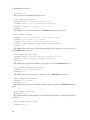
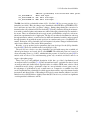
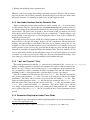
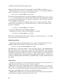
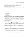
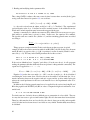
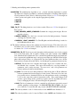
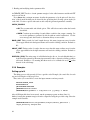
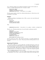
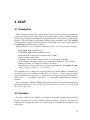
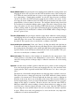
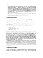
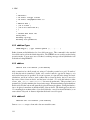
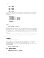
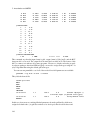
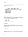
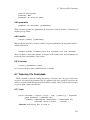
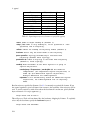
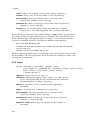
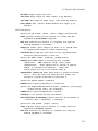
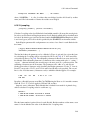
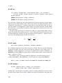
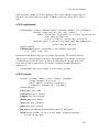
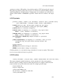
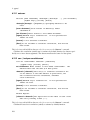
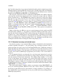
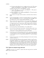
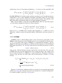
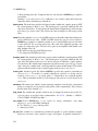
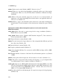
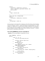
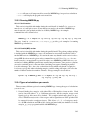
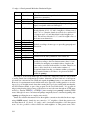
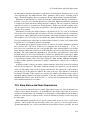
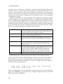
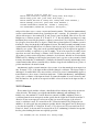
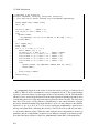
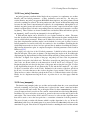
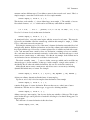
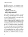
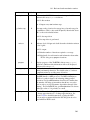
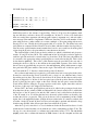
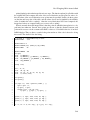
three equations:
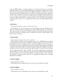
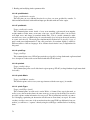
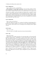
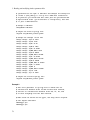
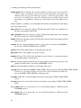
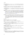
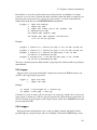
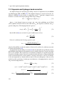
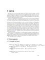
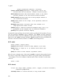
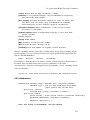
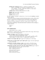
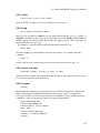
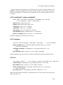
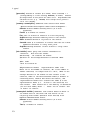
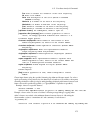
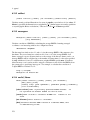
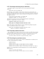
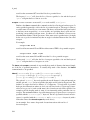
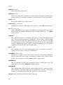
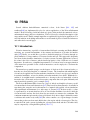
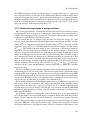
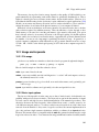
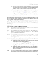
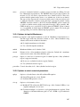
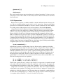
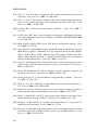
hVV (r12 , Ω1 , Ω2 ) = cVV (r12 , Ω1 , Ω2 ) + ρ V
Z
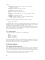
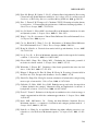
hUV (r12 , Ω1 , Ω2 ) = cUV (r12 , Ω1 , Ω2 ) + ρ V
Z
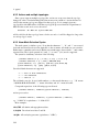
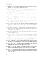
hUU (r12 , Ω1 , Ω2 ) = cUU (r12 , Ω1 , Ω2 ) + ρ V
Z
dr3 dΩ3 cVV (r13 , Ω1 , Ω3 ) hVV (r32 , Ω3 , Ω2 ),
(11.2)
dr3 dΩ3 cUV (r13 , Ω1 , Ω3 ) hVV (r32 , Ω3 , Ω2 ),
(11.3)
dr3 dΩ3 cUV (r13 , Ω1 , Ω3 ) hVU (r32 , Ω3 , Ω2 ).
(11.4)
Equation (11.3) is directly relevant for biomolecular simulations where we are often interested
in the properties of a single, arbitrarily complex solute in the solution phase. Solutions to
Equation (11.3) can be obtained using 3D-RISM. However, a solution to Equation (11.2) for
pure solvent is a necessary prerequisite and is readily obtained from 1D-RISM.
To obtain a solution to the OZ equations it is necessary to have a second equation that relates
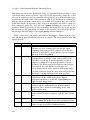
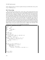
h and c or uniquely defines one of these functions. The general closure relation is[205]
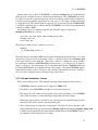
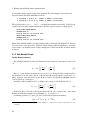
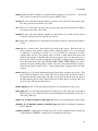
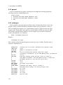
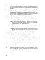
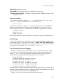
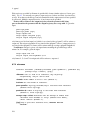
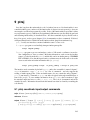
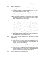
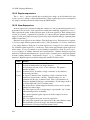
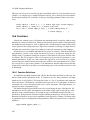
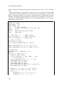
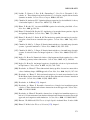
g(r12 , Ω1 , Ω2 ) = exp [−β u(r12 , Ω1 , Ω2 ) + h(r12 , Ω1 , Ω2 ) − c(r12 , Ω1 , Ω2 ) + b(r12 , Ω1 , Ω2 )]
(11.5)
u is the potential energy function for the two particles and b is known as the bridge function
(a non-local functional, representable as infinite diagrammatic series in terms of h [205]). It
should be noted that u is the only point at which the interaction potential enters the equations.
Depending on the method used to solve the OZ equations, u is generally an explicit potential.
In principle, it should now be possible to solve our two equations. For example, we may wish
to use SPC/E as a water model. Inputting the relevant aspects of the SPC/E model into u,
1D-RISM can be used to calculate the equilibrium properties of the SPC/E model. A different
explicit water model will yield different properties.
A fundamental problem for all OZ-like integral equation theories is the bridge function,
which contains multiple integrals that are readily solved only in special circumstances. In practice, an approximate closure relation must be used. While many closures have been developed,
at this time only three are implemented in 3D-RISM: hypernetted-chain approximation (HNC),
Kovalenko-Hirata (KH) and the partial series expansion of order-n (PSE-n).
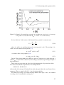
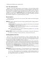
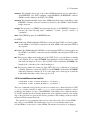
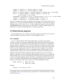
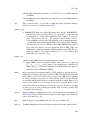
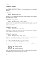
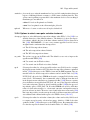
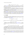
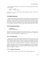
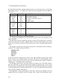
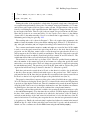
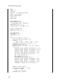
For HNC, we set b = 0, giving[205]
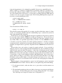
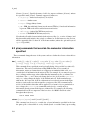
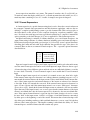
gHNC (r12 , Ω1 , Ω2 ) = exp (−β u(r12 , Ω1 , Ω2 ) + h(r12 , Ω1 , Ω2 ) − c(r12 , Ω1 , Ω2 ))
= exp (t ∗ (r12 , Ω1 , Ω2 ))
(11.6)
where t ∗ is the renormalize-indirect correlation function. HNC works well in many situations,
including charged particles, but has difficulties when the size ratios of particles in the system are
highly varied and may not always converge on a solution when one should exist. Also, as the
bridge term is generally repulsive, HNC allows particles to approach too closely, overestimating
non-Coulombic interactions[202].
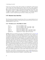
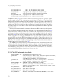
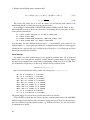
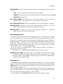
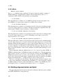
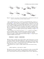
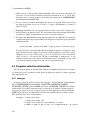
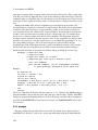
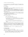
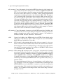
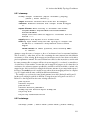
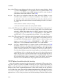
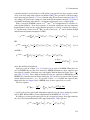
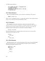
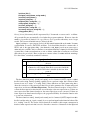
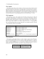
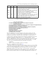
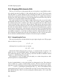
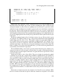
KH is a combination of HNC and the mean spherical approximation (MSA), the former being
applied to the spatial regions of solvent density depletion (g < 1), including the repulsive core,
330