1
Advanced Application 19 Construction Stage Analysis for FSM (Full Staging Method) using general functions Civ il Contents Outline.................................................................................................................. 1 Bridge profile and general section ......................................................................2 Materials & Strength .........................................................................................3 Loads ..............................................................................................................3 Composition of the Construction Stages .............................................................4 Work Environment Settings................................................................................. 6 Definition of Properties ........................................................................................ 7 Definition of Materials .......................................................................................7 Definition of Section..........................................................................................8 Definition of Time-dependent Material Properties .............................................. 11 Definition of Time-dependent Material Properties .............................................. 11 Structural Modeling............................................................................................ 13 Element Generation........................................................................................ 13 Support Generation ........................................................................................ 14 Group Definition ............................................................................................. 15 Structure Group Assignment ........................................................................... 16 Boundary Conditions Input ................................................................................ 17 Rigid Links ..................................................................................................... 17 Supports Input ................................................................................................ 18 Construction Stage Loads Input........................................................................ 19 Define Load Conditions ................................................................................... 19 Self Weight .................................................................................................... 20 Dead Load ..................................................................................................... 21 Tendon Prestress Load ................................................................................... 24 Superimposed Dead Loads ............................................................................. 29 Loading Input on the Completed Structure ....................................................... 30 Wind Loading ................................................................................................. 30 Temperature................................................................................................... 32 Live Load ....................................................................................................... 35 Differential Settlement ..................................................................................... 40 Definition of Construction Stages...................................................................... 42 Performing Structural Analysis .......................................................................... 43 Checking Analysis Results ................................................................................ 45 Element Properties & Section Properties for each Construction Stage ............... 45 Checking Construction Stage Member Forces & Stresses ................................. 47 Checking Results using Graphs ....................................................................... 50 Checking Results using Tables ........................................................................ 51 Prestress Losses ............................................................................................ 53 Checking Tendon Information .......................................................................... 54 Checking Moving Load Analysis Results .......................................................... 58 Checking Stresses due to Combined Loads ..................................................... 59 Construction stage analysis for FSM using general functions Outline FSM (Full Staging construction Method) is a very basic method in constructing posttensioned concrete bridges. Dead weight of concrete, formwork and falsework are fully shored over the full spans of a bridge until the concrete gains a certain level of strength. FSM can be economical if the horizontal alignment of a bridge is curved or the width of the bridge deck widens, provided that the height of the piers are not too high. In the case of a bridge with long spans, the use of continuous tendons can b e limited, thereby requiring construction joints. Each segment may be constructed sequentially span by span. Structural analysis is carried out on the basis of construction stages defined by the construction joints. Although a bridge is supported by sho ring, FSM is generally analyzed with the assumption that effect of support is negated by the effect of prestressing. When FSM is applied to a bridge with continuous spans, the first stage is a simple span, and it becomes continuous with the progress of the construction stages. In comparison with an analysis that does not consider construction stages, the construction stage analysis results in lower negative support moments higher positive span moments. As such, a bridge constructed by FSM needs to be an alyzed with construction stages reflecting both the change in structure, element load and boundary conditions as well as time-dependent material properties, including creep, shrinkage and modulus of elasticity. Figure 1. Bridge to be analyzed 1 ADVANCED APPLICATIONS Bridge profile and general section This example has been simplified from an actual project for the purpose of illustrating construction stage analysis using FSM. The bridge profile is defined as follows: Structure type: 3 continuous span PSC Box girder bridge (F.S.M) Spans: L = 40.0 + 45.0 + 40.0 = 125.0m Bridge width: 8.5m Skew angle: 90˚ Figure 2. Longitudinal Section 8.5 1.5 1.4 1.5 0.2 0.3 0.26 0.71 0.268 2.5 1.34 0.2 1.232 0.5 1 0.5 1.4 1.232 4.5 8.5 Figure 3. Cross Section 2 Construction stage analysis for FSM using general functions Materials & Strength ▶ Concrete 1) 2) Specified Strength: fcu 45MPa Modulus of Elasticity: Ec 3.0124 104 MPa ▶ PS Steel Tendons 1) 2) 3) Yield Strength: f py 1580MPa Tensile Strength: f pu 1860MPa 2 Nominal Sectional Area: Ap 100cm 5) 5 Modulus of Elasticity: E p 1.95 10 MPa Initial Prestressing Force: f pj 0.75 f pu 1395MPa 6) Anchorage Slip: 7) 8) Coefficient of Curvature Friction : 0.25 / rad Coefficient of Wobble Friction: k 0.0066/ m 4) s 6mm Loads ▶ Primary loads and special loads pertaining to the primary loads 1) Dead Loads A. Reinforced Concrete: 24.52kN / m2 B. Asphalt Concrete: 22.56kN / m2 C. Barriers and safety fences D. Prestress, creep, shrinkage 2) Live Loads A. Vehicle Loads: Types HA and HB Loading 3) Differential settlements : The worst combination of each pier settlement of 10mm ▶ Secondary loads 1) Temperature A. For total deformation (±15˚) 2) Wind B. Temperature differential between top & bottom chords (±5˚) 3 ADVANCED APPLICATIONS Composition of the Construction Stages This figure below represents the entire construction stage process. Construction stages are generated excluding the erection of the shoring and temporary bents themselves, which have no effect on the structure. Figure 4. Construction Stage Chart The following construction stages are reflected in the analysis. CS1 (30 days) CS2 (30 days) CS3 (30 days) CS4 (10,000 days) 4 Construction stage analysis for FSM using general functions Figure 5. Tendon Placement Layout 5 ADVANCED APPLICATIONS Work Environment Settings For FSM construction stage analysis, open a new file, ( as ( Save) ‘FSM.mcb’. New Project), and save Select ‘kN’ and ‘m’ for the unit system. The unit system can be conveniently changed at any time later depending on your preferred types of input data. / New Project / Save (FSM) Tools / Unit System Length> m ; Force>kN The unit system can be changed by clicking “Unit Selection” ( ) on the Status Bar at the bottom of the screen. Figure 6. Unit System Setting 6 Construction stage analysis for FSM using general functions Definition of Properties Definition of Materials Define the material of the PSC box by selecting one from the built-in database. The material for tendons can be defined using the User Defined function. Properties / Material Properties Click Type>Concrete DB>C45 Apply ; Standard>BS(RC) Name>Tendon ; Type>User Defined Modulus of Elasticity (1.95e8) Weight Density (78.5) The tendon weight is automatically accounted for after grouting. Figure 7. Material Data Input Dialog Box 7 ADVANCED APPLICATIONS Definition of Section Refer to the cross section dimensions in Figure 8 to define the section of the PSC box. Properties / Click Section Properties PSC tab Section ID (1) ; Name (Span) PSC-1CELL, 2CELL Joint On/Off>JO1 (on), JI1 (on), JI3 (on), JI5 (on) Web Thick> for Shear t1 (on), t2 (on), t3 (on), for Torsion(min) (on) Offset>Center-Top Outer HO1 (0.2) ; HO2 (0.3) ; HO2-1 (0) ; HO3 (2.5) BO1 (1.5) ; BO1-1 (0.5) ; BO2 (0.5) ; BO3 (2.25) Inner HI1(0.24) ; HI2(0.26) ; HI2-1(0) ; HI3(2.05) ; HI3-1(0.71) HI4 (0.2) ; HI4-1 (0) ; HI5 (0.25) BI1(2.2) ; BI1-1(0.7) ; BI2-1(2.2) ; BI3(1.932) ; BI3-1(0.7) Or click to enter the input data in a table. 2.2 0.7 0.2 0.3 0.24 0.26 0.5 0.71 2.05 2.5 1.932 0.7 0.2 0.25 1.5 0.5 2.25 Figure 8. Input Data for the Cross Section 8 Construction stage analysis for FSM using general functions Checking on “Mesh Size for Stiff Calc.” enables us to define a maximum size of mesh, which is used to calculate the section properties. “Consider Shear Deformation” accounts for shear deformation. Figure 9. Section Input Dialog Box Cross sectional dimensions can be entered via a table upon clicking for the PSC section. This is faster than directly entering the data in the dialog box for a large amount of dimensional data. The table is compatible with Excel. Frequently used cross sectional dimensions can be saved to copy & paste later. The table becomes compatible with Excel by entering “0” for Check Off ( ) and “1” for Check on ( ). Figure 10. Table Input (PSC) 9 ADVANCED APPLICATIONS Shear Check Assign the locations for shear calculations on the PSC section. Numerical data can be entered manually, or if “Au to” is selected, shear calculations take place at the top and bottom of the web(s). The shear results are displayed in no. 5~10 of the Beam Stress (PSC). Web Thick. for Shear(total) Enter the thicknesses to be used for shear calculations at the locations defined for Shear Check at Z1 through Z3. Enter the sum of web thicknesses at a given location. Check on “Auto” for automatic calculations. for Torsion(min.) Enter a minimum thickness for torsion calculation. 10 Construction stage analysis for FSM using general functions Definition of Time-dependent Material Properties Define the time-dependent properties of the concrete (creep coefficients shrinkage and strength). Properties / Time Dependent Material / Creep/Shrinkage Click ; Name>C45 ; Code>CEB-FIP(1990) Compressive strength of concrete at the age of 28 days (45000) Relative Humidity of ambient environment (40-99) (70) Notational size of member (0.364) Type of cement>Normal or rapid hardening cement (N, R) Age of concrete at the beginning of shrinkage (3) Properties / Time Dependent Material / Comp. Strength Click ; Name>C45 ; Code>CEB-FIP Concrete Compressive Strength at 28 Days (45000) Type of cement>N, R : 0.25 Figure 11. Time Dependent Material Data 11 ADVANCED APPLICATIONS Link the time dependent material properties to the material properties. The creep coefficients, shrinkage and concrete strength curves defined earlier need to be linked to the corresponding material property in order to carry out construction stage analysis reflecting their effects. Properties / Time Dependent / Material Link Time Dependent Material Type Creep/Shrinkage>C45 Comp. Strength>C45 Select Material for Assign>Materials> 1:C45 Selected Materials Figure 12. Linking Time Dependent Material Property to the Material Property. 12 Construction stage analysis for FSM using general functions Structural Modeling Element Generation Generate a girder using the “Extrude” function. Node/Element / Create Nodes Coordinates (x, y, z) (0, 0, 0) Node/Element / Extrude Select All Extrude Type>Node -> Line Element Element Attribute Element Type>Beam Material>1: C45 Section>1: Span Translation > Unequal Distance Axis>x Distances ([email protected], 5@2, [email protected], 5@2, [email protected]) Zoom Fit Figure 13. Girder Generation 13 ADVANCED APPLICATIONS Support Generation Considering the spans (40+45+40), create nodes to which boundary conditions will be assigned. Since the depth of the girder is 3m, and the distance between the bearings is 3m with the working point being Center-Top, the supports are created at Z=-3m & Y=±1.5m. Node/Element / Create Nodes Start Node Number Node Numbering Option>User-Defined Number Newly Created Number (61) Coordinates (x, y, z) (0, 1.5, -3) Copy Number of Times (1) Distances (dx, dy, dz) (0, -3, 0) Node/Element / Translate Node Select Recent Entities Mode>Copy Translation Unequal Distance Axis>x Distance (40, 45, 40) Figure 14. Generation of Support Nodes 14 Construction stage analysis for FSM using general functions Group Definition Refer to “Construction Stage Configuration” on Figure 4 for the list of the groups to be defined. Structure / Group / Structure Name (SG) ; Suffix (1to3) Structure / Group / B/L/T / Define Boundary Group Name (BG) ; Suffix (1to3) Tendon Group is not used for composing the construction stages, but is defined to check the results for each group. Structure / Group / B/L/T / Define Load Group Name (Dead) ; ; Name (Superimposed Dead) ; Name (PS) ; Suffix (1to3) ; Name (Diaphragm) ; Suffix (1to3) ; Structure / Group / B/L/T / Name (A) ; Name (B) ; Name (C) ; Define Tendon Group Suffix (1to4) Suffix (1to4) Suffix (1to4) Refer to the name assignment of the “Tendon Profile” to see the items of the Tendon Group. Figure 15. Group Generation 15 ADVANCED APPLICATIONS Structure Group Assignment Assign the elements, which will be activated at each stage, to SG1~3 respectively. Assign the elements to Structure Group by using “Drag & Drop,” or by right-clicking and selecting “Assign”. Elements Numbers ; Front View Group Tab in the Tree Menu Type the numbers of nodes and elements as below Select Nodes : 61to64 & Elements : 1to20 Structure Group > SG1 Drag & Drop or (Context Menu) Assign Select Nodes : 65to66 & Elements : 21to39 Structure Group > SG2 Drag & Drop or (Context Menu) Assign Select Nodes : 67to68 & Elements : 40to52 Structure Group > SG2 Drag & Drop or (Context Menu) Assign [SG1] Node : 61to64 & Element : 1to20 [SG2] Node : 65to66 & Element : 21to39 [SG3] Node : 67to68 & Element : 40to52 Drag & Drop Figure 16. Structure Group Assignment 16 Construction stage analysis for FSM using general functions Boundary Conditions Input Rigid Links Considering the centroid of the cross section of the PSC Box, rigid links are connected to the supports. Iso View Boundary / Elastic Link Boundary Group>BG1 Link Type>Rigid Type 2Nodes (1, 61) ; (1, 62) ; (18, 63) ; (18, 64) Boundary Group>BG2 2Nodes (37, 65) ; (37, 66) Boundary Group>BG3 2Nodes (53, 67) ; (53, 68) Turn on the node number if necessary when picking up nodes Figure 17. Rigid Links 17 ADVANCED APPLICATIONS Supports Input Considering the construction stages, the supports are defined as below. Top View ; Redraw Boundary / Define Supports Boundary Group>BG1 Select Single (Node : 61 ) Select Single (Node : 62 ) Select Single (Node : 63 ) Select Single (Node : 64 ) ; Support Type>Dy (on), Dz(on) ; Support Type>Dz(on) ; Support Type>Dx(on), Dy(on), Dz(on) ; Support Type>Dx(on), Dz(on) Boundary Group>BG2 Select Single (Node : 65 ) ; Support Type>Dy(on), Dz(on) Select Single (Node : 66 ) ; Support Type>Dz(on) Boundary Group>BG3 Select Single (Node : 67 ) ; Support Type>Dy(on), Dz(on) Select Single (Node : 68 ) ; Support Type>Dz(on) BG1 BG1 BG2 Figure 18. Boundary Condition Input 18 BG3 Construction stage analysis for FSM using general functions Construction Stage Loads Input Define Load Conditions Define load cases for analysis. We take the time to define the load “Type” then we can take advantage of the ability to automatically generate load combinations using the "Auto Generate” function. Using these Types of load case we may generate the load combinations after application of the load factors as per the design standard. Redraw Load / Static Load Cases Name (Self Weight) Name (Non-Structure Dead) Name (Prestress) Name (Superimposed) Name (Wind) Name (Temperature (+)) Name (Temperature (-)) Name (Top-Bot Temp Diff(+)) Name (Top-Bot Temp Diff(-)) ; Type>Construction Stage Load (CS) ; Type>Construction Stage Load (CS) ; Type>Construction Stage Load (CS) ; Type>Construction Stage Load (CS) ; Type>Wind Load on Structure (W) ; Type>Temperature (T) ; Type>Temperature (T) ; Type>Temperature Gradient (TPG) ; Type>Temperature Gradient (TPG) Figure 19. Load Cases Definition 19 ADVANCED APPLICATIONS Self Weight Enter the self weight. Define the structure’s self weight and activate it at the first construction stage. Then the self weights of the elements activated in the subsequent construction stages will automatically be applied. Load / Self Weight Load Case Name>Self Weight Load Group Name>Dead Self Weight Factor>Z (-1) Figure 20. Self Weight Input 20 Construction stage analysis for FSM using general functions Dead Load Enter diaphragms and construction joint blocks, as loads as they have not been reflected in the model. Front View Load / Element Beam Loads Select Elements by Identifying (1, 52) Load Case Name>Non-Structure Dead Direction>Global Z Relative x1(0) ; x2 (1) ; w(-220.34) Select Elements by Identifying (19to21, 38to40) Relative x1(0) ; x2 (1) ; w(-63.0) Select Elements by Identifying (16, 35) Absolute x1(1.5) ; x2 (2.5) ; w(-220.34) Select Elements by Identifying (17, 36) Absolute x1(0) ; x2 (1) ; w(-220.34) Figure 21. Miscellaneous Dead Loads 21 ADVANCED APPLICATIONS Figure 22. Dead Load Layout The diaphragms at the supports and the construction joint blocks have not been considered as structural elements in this longitudinal analysis and are thus treated as loads. Their cross sectional areas are calculated and converted into Beam Load over the corresponding lengths. Other additional dead loads may exist, but are ignored in this Tutorial. Diaphragm (End: 2m, Intermediate Support: 2.5m) Area 9.941m2 0.955m2 8.986m2 P 8.986m2 24.52kN / m3 220.34kN / m Construction Joint Block Area 1.288m2 2EA 2.576m2 P 2.576m2 24.52kN / m3 63kN / m We need to assign the loads to Load Groups and activate the Load Groups in the corresponding construction stages. Because the magnitudes of the Beam Loads are the same, setting the Load Group to 22 Construction stage analysis for FSM using general functions Default is convenient for input. We will now see how to modify the Load Group using the Table Tab. By selecting the desired columns, we can adjust the locations in Beam Load Table. The row column containing the Group information is located at the end of the Table. For convenience, we will select the entire column, and move it next to the Element numbers. Assign Load Group: Diaphragm1 to 3 to the loads in order to activate them in Stages 1 through 3. Load / Load Tables / Static Load / Assign Element 1~20> Diaphragm1 Element 21~39>Diaphragm2 Element 40~52>Diaphragm3 Beam Loads Note that the Group column is found at the last column in the table as shown in the first figure of the three figures below. In the second figure, the Group column was relocated to the front for convenience. The third figure depicts how Diaphram is applied to the elements. Figure 23. Changing Load Group using Table 23 ADVANCED APPLICATIONS Tendon Prestress Load Define the properties of the Tendon related to the material, strength, losses. etc Load / Temp./Prestress / Click Relaxation Coefficient can be defined by selecting Magura equation, JTG04 or CEB-FIP Code. Tendon Property Tendon Name (Tendon) Tendon Type> Internal(Post-Tension) ; Material> 2: Tendon Total Tendon Area> 0.0016112 or Strand Diameter> 12.9mm(1χ3) ; Number of Strands> 19 Duct Diameter (0.1) Relaxation Coefficient> CEB-FIP(2.5%) Ultimate Strength> (1860000) ; Yield Strength> (1580000) Curvature Friction Factor> (0.25) ; Wobble Friction Factor> (0.0066) Anchorage Slip(Draw in)> Begin(0.006) , End(0.006) Bond Type> Bonded If “Unbonded” is selected, the section stiffness is calculated on the basis of the net cross section. “Bonded” reflects the composite stiffness reflecting the tendons. Figure 24. Tendon Property Dialog 24 Construction stage analysis for FSM using general functions The Tendon Profile can be defined in many ways such as defining the inflection points, but this example uses a common approach often used in practice, using the Tendon ordinates from drawings. Referring to the values in the attached Excel file (TD profile.xls), prepared on the basis of the tendon drawings the ordinates of the tendon at every 2m are pasted into the software. Copy & Paste the values from the Excel file to enter the Profile. We may also copy the Profile after creating an MCT file. Load / Temp./Prestress / Tendon Profile Tendon Name (A1L) ; Group (A1) Tendon Property> Tendon ; Assigned Elements (1to20) Input Type> 3-D ; Curve Type> Spline Profile 1> x (0), y (0), z (-1) 2> x (2), y (0), z (-1.2590) … 25> x (48), y (0), z (-1.25) Profile Inserton Point> End-I of Elem.1 x Axis Direction> I->J of Elem.1 ; x Axis Rot. Angle (-11.3) Offset y : (2.666) Transfer Length may be specified to consider the unstressed length of the anchorage. Checking on “Typical Tendon” and entering the number of tendons can be used to represent a number of tendons of the same profile. This is also handy when preliminary analysis is undertaken. Figure 25. Tendon Profile Input Dialog 25 ADVANCED APPLICATIONS From the tendon profile drawings, x-z coordinates are obtained at every 2m. The result (TD Profile.xls) contains the values as if the tendons were placed in the centroidal 2-D plane, each side. We need to translate the layout using y-Offset and rotate the layout using x-Rotation to properly position them in the webs of the PSC section. Figure 26. 3-Dimentional Tendon Profile Input Copy and paste the values of x, y and z from the Excel file as below, and position the tendons in the webs by y-Offset and x-Rotation depending on the “left” or “right” tendon. 26 Construction stage analysis for FSM using general functions The Name and the Assigned Elements for all Tendon Profiles are as follows: Ex) A1L X coordinate (A, B, C), Z coordinate (1, 2, 3, 4), Y coordinate (Left, Right) Figure 27. Name Assignment for Tendon Profile Tendon Profile A1, A2 B1, B2 C1, C2 Assigned Element 1 ~ 20 21 ~ 39 40 ~ 52 Tendon Profile A3, A4 B3, B4 C3, C4 Assigned Element 1 ~ 20 19 ~ 39 38 ~ 52 Figure 28. Result of Tendon Profile Input 27 ADVANCED APPLICATIONS After defining all the Tendon Profiles, assign the Load Groups (PS1~3) and then apply prestress loads so that the defined Tendon Profiles can be applied to each construction stage. Prestress is applied one stage after the stage at which the load is entered. Load / Temp.Prestress / Tendon Prestress Loads Load Case Name> Prestress Load Group Name> PS1 Select Tendon for Loading Tendon> A1L~A4R Stress Value Begin (1395000) ; End (0) Grouting: after (1) Stage Load Group Name> PS2 Select Tendon for Loading Selected> A1L~A4R ; Tendon> B1L~B4R Load Group Name> PS3 Select Tendon for Loading Selected> B1L~B4R ; Tendon> C1L~C4R Figure 29. Loading Tendon Prestress 28 Construction stage analysis for FSM using general functions Superimposed Dead Loads Superimposed Dead Loads are applied as Beam Load onto the superstructure. Barriers (0.3075m2 0.4975m2 ) 24.52kN / m3 Safety Fences 19.74kN / m 1kN / m Asphalt concrete pavement 7.5m 8cm 22.56kN / m Noise barriers 1 3 . 5 3k 6N m/ 1.52kN / m Total 35.796kN / m 3 Load / Static Loads / Beam Loads/ Element Select All Load Case Name>Superimposed Load Group Name> Superimposed dead Load Type>Uniform Loads Value Relative ; x1(0) ; x2 (1) ; w(-35.796) Figure 30. Loading Superimposed dead Loads 29 ADVANCED APPLICATIONS Loading Input on the Completed Structure Wind Loading wind loading of 3 kN/m 2 3 kN/m 2 1.46 Figure 31. Wind Load Distribution Total Height = Section Depth + Barriers + Noise barriers = 3 + 1 + 2.5 = 6.5m Wind Pressure= 3kN / m2 Wind Load = 6.5m 3kN / m2 19.5kN / m (Horizontal Load) = 19.5kN / m 1.46m 28.47kN m / m (Eccentricity Moment) 30 Construction stage analysis for FSM using general functions Enter the wind loads. Load / Static Loads/ Beam Loads / Loading pertaining to the Load Groups, which are not activated during the construction stages, are loaded in PostCS. Element Select All Iso View Load Case Name>Wind Load Group Name>Default Load Type>Uniform Loads Direction>Global Y Value Relative x1(0) ; x2 (1) ; w(19.5) Select All Load Type>Uniform Moments/Torsion Direction>Global X Value Relative x1(0) ; x2 (1) ; w(-28.47) Figure 32. Wind Loading Input 31 ADVANCED APPLICATIONS Temperature Specify the temperature loading acting on the entire structure. The System Temperature function allows us to specify strain, t (T2 T1) , over the entire structure as temperature loads. Load / Temp./Prestress / Temperature Loads / Redraw Load Case Name>Temperature (+) Load Group Name>Default Temperature > Final Temperature (15) Load Case Name>Temperature (-) Load Group Name>Default Temperature > Final Temperature (-15) System Temp. Figure 33. Temperature Loading Input 32 Construction stage analysis for FSM using general functions Specify the differential temperature between the top and bottom chords. The Beam Section Temperature function generates a temperature differential between top and bottom chords on a part of a rectangle. Since PSC sections are not rectangular sections, they need to be converted into equivalent rectangular sections to be able to specify temperature differential loads. Where temperature differentials exist as shown below, the parts experiencing the temperature differentials are converted into a rectangle defined by dotted lines having the same area and centroid. Beam Section Temperature can be defined as either General Type or PSC Type. General Type assumes the section as a rectangle. When PSC Type is specified, the sections defined as PSC Type in defining Section Data are automatically converted into rectangles and loaded on the parts experiencing temperature differentials. Although the Beam Section is defined as PSC Type in this example, which results in a simple input process for loading for a temperature differential between the top and bottom chords, input is carried out as General Type after converting into a rectangle. Figure 34 shows the calculations for cross sectional area and centroid of the top part of the PSC Box section using SPC (Section Property Calculator). The instruction for using SPC is separately documented in user’s manual. Figure 34. Section Properties calculated by SPC 33 ADVANCED APPLICATIONS Using the above calculation results in conversion into an equivalent rectangle, which will be loaded, as follows: Area = 2.896m2 H = 2 0.312977m 0.625954m B Area 2.896 4.626m H 0.625954 Load / Temp./Prestress / Temperature Loads / Beam Section Temp. Load Case Name> Top-Bot Temp Diff (+) Load Group Name>Default Direction > Local-z ; Ref. Position > Centroid B (4.626) ; H1 (0.71) ; H2 (1.336) ; T1 (5) ; T2 (5) Select All Delete the defined Section Temperatures (select ①and delete) Load Case Name> Top-Bot Temp Diff (-) B (4.626) ; H1 (0.71) ; H2 (1.336) ; T1 (-5) ; T2 (-5) Select All ① Figure 35. Input for Temperature Differential between Top & Bottom Chords 34 Construction stage analysis for FSM using general functions Live Load The sequence of defining the live load is as follows: Select a Code defining live load: Define Moving Load Code Define lanes: Traffic Line Lanes Define vehicles: Vehicles Define live load cases: Moving Load Cases ▶ Select a Code, which specifies live load The input process and the parameters are tailored to the selected Code. Load / Moving Load Load Type / Moving Load Code Moving Load Code>BS ▶ Define traffic lanes Eccentric and symmetrical loading can be considered for the transverse position of traffic lanes. In this tutorial, we specify only a symmetrical loading case as described below. The eccentricity is positive (+) if the traffic lane (center) is on the right side of the elements in the direction of traffic, and vice versa. Since this example bridge is straight and symmetrical, only the wind loading in the +Y direction has been applied. For the worst condition, only the eccentric live load in the +Y direction is entered. Figure 36. Traffic Lanes & Eccentricities 35 ADVANCED APPLICATIONS Refer to the Figure 36 for the traffic lanes and eccentricities to define 2 traffic lanes. Top View W h en a traffic lane i s c urve d or whe n the l ane data entry with 2 P oi nts becomes aw kward due to di s continuity, select “Nu mber” and di r e ctly type in the e l e ment numbers. (In t h i s case, even if you s e l ect “Number” and i npu t “1 to 53”, the Load / Moving Load / Traffic Line Lanes Click Lane Name (Lane 1 left) Traffic Lane Properties Eccentricity (-1.75) ; Wheel Spacing (1) Vehicular Load Distribution > Lane Element Selection by > 2 Points ((0, 0, 0)(125, 0, 0)) Click OK Click Lane Name (Lane 2 right) Traffic Lane Properties Eccentricity (1.75) ; Wheel Spacing (1) Vehicular Load Distribution > Lane Element Selection by > 2 Points ((0, 0, 0)(125, 0, 0)) Click OK ; Lane Width(3.5) ; Lane Width(3.5) s ame traffic lanes are s e l ected) Figure 37. Traffic Lane Input Dialog & Input Result 36 Construction stage analysis for FSM using general functions ▶ Definition of Vehicle Loads Define the vehicles for live loads. Load / Moving Load Analysis Data / MIDAS/Civil contains the standard vehicle loads such as BS Vehicles Standard Name > BD 37/01 Standard Load Vehicular Load Name > HA & HB(Auto) Vehicular Load Type > HA & HB(Auto) 5400, BS BD 37/01, AASHTO Standard, AASHTO LRFD, Caltrans, etc. Figure 38. Definition of Vehicle Loads Figure 39. Definition of BD37/01 Standard Vehicular Load 37 ADVANCED APPLICATIONS ▶ Conditions for applying live loads To consider Load Cases, which combines the effects of HA and HB vehicle , Load case name MV U 1, MV U 2 3, MV S 1 and MV S 2 3 are created as below. Type of Design Combination Factor L oad factors for H A l oading for ULS, S L S , Combination 1 and Combinations 2 & 3 ar e taken from S e c tion 6.2.7 of BD 37/ 01. Load factors Load Case Name Ultimate Limit State Serviceability Limit State Combination 1 Combination of Loads Combination 2 & 3 MV U 1 MV S 1 MV U 2 3 MV S 2 3 for HB loading for U L S, SLS, Combi nation 1 and Combi nations 2 & 3 ar e taken from S e c tion 6.3.4 of BD 37/ 01. These load fac tors are au t omati cally i nc orporated into movi ng load analysis r e s ults. Th erefore , to avoi d du plication, the u s e r shoul d not apply t h e load factors for movi ng loads while ge ne rating the Load Combi nations. Table 1. Definition of Load Case Name Load / Moving Load Analysis Data / Moving Load Cases Click Load Case Name (MV U 1) Check on Auto Live Load Combination Type of Design Combination Factor>Ultimate Limit State Combination of Loads>Combination 1 Load Case Data Scale Factor field (1) ; Number of Loaded Lanes (2) Vehicle>HA & HB (Auto) Assignment Lanes List of Lanes (Lane 1 left, Lane 2 right) Selected Lanes Load Case Name (MV U 2 3) Type of Design Combination Factor>Ultimate Limit State Combination of Loads>Combination 2 or 3 38 Construction stage analysis for FSM using general functions Figure 40. Definition of Live Load 39 ADVANCED APPLICATIONS Differential Settlement ▶ Definition of Differential Settlement Groups Select the nodes, which can settle simultaneously, representing the abutments and piers, to individually define them as a Settlement Group. Load / Settlement/Etc. / Settlement Group Group Name > A1 ; Settlement Displacement (-0.01) Select By Window (61, 62) Group Name > P1 ; Settlement Displacement (-0.01) Select By Window (63, 64) Group Name > P2 ; Settlement Displacement (-0.01) Select By Window (65, 66) Group Name > A2 ; Settlement Displacement (-0.01) Select By Window (67, 68) Figure 41. Definition of Differential Settlement Groups 40 Construction stage analysis for FSM using general functions ▶ Conditions for Differential Settlement Loads Using the data for differential settlement groups, the loading condition is defined. Ma ximum/Minimum numbers of differential settlement groups are specified. Min: 1 support and Max: 3 supports are specified to investigate all the possible combinations of simultaneous settlements from which Min/Max results are produced. Since the magnitude of the settlements of all 4 Load / Settlem ent/Etc. / Settlement Load Case Load Case Name (SM) Select Settlement Group Settlement Group (A1, P1, P2, A2) Selected Group Smin (1) ; Smax (3) groups is identical, only a maximum of 3 combinations is used. Figure 42. Definition of Loading Conditions for Differential Settlements 41 ADVANCED APPLICATIONS Definition of Construction Stages We refer to the composition of construction stages outlined earlier to define the stages. Load / Construction Stage / Define C.S Name> CS1 Duration>30 Element tab Group List>SG1 ; Activation>Age ( 5 ) Boundary tab Group List>BG1 Activation>Spring/Support Position>Deformed (on) Load tab Group List>Dead, PS1, Diaphragm1 Activation>Active Day>First Concrete maturity (age) of 5 days is activated. Stage (days) Element Boundary Load CS1 30 SG1 BG1 Dead, PS1, Diaphragm1 CS2 30 SG2 BG2 PS2, Diaphragm2 CS3 30 SG3 BG3 PS3, Diaphragm3 CS4 10,000 - - Superimposed dead Figure 43. Dialog Boxes for defining Construction Stages 42 Construction stage analysis for FSM using general functions Performing Structural Analysis Select the analysis options for construction stage analysis and moving load analysis and perform analysis. Construction Stage Analysis All the dead loads applied during the construction stages are included in CS:Dead Load. If results for other Load Cases need to be separated from CS:Dead Load, such Load Cases need to be selected in “Load Cases to be Distinguished from Dead Load for C.S. Output”. Separate results are then produced in CS:Erection Load. Analysis / Construction Stage Analysis Control Check on “Save Load Cases to be Distinguished from Dead Load for C.S. Output Load Case>Superimposed Save Output of Current Stage(Beam/Truss) (on) Output of Current Stage (Beam /Truss)” to produce member forces generated only from each (current) stage. That is, not the member forces accumulated up to that (current) stage. Checking on “Change with Tendon” in “Beam Section Property Change” will reflect the effect of Figure 44. Construction Stage Analysis Control Data tendons for calculating section properties by construction stages. 43 ADVANCED APPLICATIONS Moving Load (Live Load) Analysis Specify the number of points per beam element on which influence line is calculated. A number between 1 to 10 can be specified. Select the method of influence line calculation and the options for generation of analysis results. Analysis / Moving Load Analysis Control Influence Generating Method > Number/Line Element (2) Analysis Results Frame>Normal + Concurrent Force Combined Stress Calculation (off) “Concurrent Force” will generate member forces, which take place simultaneously under the same loading. Check on “Combined Stress” to generate combined stress results. A substantial amount of results are generated from moving load analysis. Only the desired parts should be selected in groups for output generation. Figure 45. Moving Load Analysis Control Dialog Execution of Structural Analysis We have completed the process of structural modeling and defining the analysis options, so analysis can begin now. Analysis / 44 Perform Analysis Construction stage analysis for FSM using general functions Checking Analysis Results Construction stage analysis results will be reviewed via the versatile functionality of midas Civil. Element Properties & Section Properties for each Construction Stage The properties of each element used during the construction stages are produced in a table. Select a stage to see the corresponding data; initial (Start) age, final (End) age, initial (Start) modulus of elasticity, final (End) modulus of elasticity, shrinkage accumulated up to the end of the corresponding stage and creep coefficient. When a construction stage is selected, only the results pertaining to the corresponding stage are produced. The Post CS construction stage is selected followed by pressing the button to change the result values as below. Results / Result Table / Construction Stage / Element Properties at Each Stage PostCS (Post construction stage) Figure 46. Element Properties at each Construction Stage 45 ADVANCED APPLICATIONS Transformed section properties used in the last stage of the construction stage analysis are produced in a table. The properties may change with change in modulus of elasticity (if a time dependent material is used). And if tendons are included in sections, the tendon properties and the timing of grouting will affect the section properties. * In order to reflect the Tendon in section property calculations, “Change with Tendon” needs to be selected in Construction Stage Analysis Control. * If “Change with Tendon” is selected, and “Bonded” type in “Tendon Property” is selected, the Tendon will be reflected in the section property calculations. Otherwise (in case of “Unbonded”), the Tendon is excluded and the net section is used in the calculations. The section properties at the last stage are used for calculating stresses due to additional loads applied at the completed stage such as moving load, temperature load, wind load, etc. Results / Result Table / Construction Stage / Beam Section Properties at Last Stage In t h e *.out fil e, w e c an see the s e c tion properties for all the stages in addi tion to those for t h e final stage. Figure 47. Section Property Data at the Last Stage 46 Construction stage analysis for FSM using general functions Checking Construction Stage Member Forces & Stresses Member forces can be checked in a diagram using the Beam Diagram function. If a beam element is selected after invoking Quick View, member forces at any particular point on the selected element can be checked in detail. Results / Forces / Beam Diagrams… CS4 Load Cases/Combinations>CS:Summation ; Step>Last Step Components>My Display Options> Solid Fill Type of Display Contour (on) ; Legend (on) Type of Display>Quick View Figure 48. Checking Member Forces at CS4 47 ADVANCED APPLICATIONS Using the Beam Stresses(PSC) function, the stresses in a PSC section can be checked in a diagram. A total of 10 locations, Top/Bot vetices (1 to 4), Center (7 & 8) and shear checking points (5, 6, 9 & 10) defined at the time of defining the PSC section, can be checked. Let us check the bottom chord stress for CS:Summation at the last construction stage. Results / Stresses / Beam Stresses(PSC)… CS4 Load Cases/Combinations>CS:Summation ; Step>Last Step Section Position>Position 3 Components>Sig-xx(Summation) Type of Display Contour (on) ; Legend (on) Top-Bot chord stresses for each construction stage can be also checked in Bridge Girder Diagram. In case of a PSC section, Beam Stresses (PSC) can be used to check Contour in the Model View state. Figure 49. Bottom Chord Stresses at the Last Stage 48 Construction stage analysis for FSM using general functions Using User Defined Diagram, different results (displacements / member forces / stresses) for different elements/groups can be produced. We will generate results for displacements in the left span, bending moments in the middle span and stresses in the right span in a single diagram simultaneously. Let us check displacements / member forces / stresses for CS:Summation at the last construction stage. Combined results can be produced only in the same construction stage. Output option can be selected in Results / Diagram / Define Diagram… CS4 Element>1to16 ; Type of Result>Displacement Component>DZ ; Group Name>Disp Element>17to35 ; Type of Result>Beam Force/Moments Component>My ; Group Name>Force Element>36to52 ; Type of Result>Beam Stresses(PSC) Section Position>Abs Max ; Components>Sig-xx(Summation) Group Name>PSC Stress Results / Diagram / Plot Diagram… Load Cases/Combination>CS: Summation Diagram Group>Disp(on), Force(on), PSC Stress(on) < Displacement > < Moment > < Stress > Note that the three plots above have different scale factors to properly display in this figure. In order to check the results, you may enlarge the figure and compare the values. Figure 50. User Defined Diagram Output Display 49 ADVANCED APPLICATIONS Checking Results using Graphs The change in stresses with the progress of construction stages in the suppo rt element (No.36) will be checked in a Graph. Results / Stage/Step History Graph CS4 Define Function>Beam Force/Stress Name(36_ax) ; Element No.(36) ; Stress Point>I-Node ; Components>Axial Name(36_b(+y)) Name(36_b(-y)) Name(36_b(+z)) Name(36_b(-z)) If “Multi LCase” is selected, the results history of the component of ; Components>Bend(+y) ; Components>Bend(-y) ; Components>Bend(+z) ; Components>Bend(-z) Mode >Multi Func. Step Option>All Steps Load Cases/Combinations>Summation the corresponding element for a number of Load Cases can be checked. Figure 51. Change in Stresses with Construction Stages 50 Construction stage analysis for FSM using general functions Checking Results using Tables Tables are also useful in checking construction stage analysis results. manipulated in various ways by right-clicking on the tables. Tables can be From “Records Activation Dialog”, tables can be generated by selecting elements to be checked for stresses, load cases, construction stages (steps), elements on which points of stress output are required, load cases, construction stages (steps), stress output locations on elements, stress output locations on a section, etc. The Sorting Dialog allows us to sort/arrange the data based on the sorting criteria. The Style Dialog allows us to change the data type and produce results. Let us check top vertex stresses for CS:Summation at the last construction stage. Results / Result Tables / Beam / Stresses(PSC) Figure 52. Checking Top Chord Stresses using Table 51 ADVANCED APPLICATIONS In “Construction Stage Analysis Control” dialog box, if “Sa ve Output of Current Stage (Beam/Truss)” option has been checked on, we can generate the member forces resulting only from the corresponding construction stage (not the member forces accumulated up to that stage). So in order to produce results for the un-accumulated effects of one given construction stage, check “Current Step Result” for all the stages. Results / Result Tables / Beam / Force Figure 53. Member Forces due to the sole effect of Current Stage (below) 52 Construction stage analysis for FSM using general functions Prestress Losses We can check the change in tendon tension at each construction stage due to prestress losses. In the “Tendon Time Dependent Loss Graph” dialog box, only the tendons included in the stage selected in the “Stage” selection window can be checked. A Graph is generated for selected tendons, selected Stage and selected Step. Click to check the results in an animation. Results / Tendon Time-dependent Los s Graph Tendon>A1L Figure 54. Graph showing Loss of Prestress Forces 53 ADVANCED APPLICATIONS Checking Tendon Information The tendon information used in construction stage analysis can be produced in a table. The coordinates of the tendons placed in elements are produced. Results / Result Tables / Tendon / Tendon Coordinates… Figure 55. Tendon Coordinates Table Elongation of tendons is produced. Timing of tensioning each tendon, elongation of tendons and elements at the start and end points of the tendons and their sum are produced. Results / Result Tables / Tendon / Tendon Elongations… Figure 56. Tendon Elongation Table 54 Construction stage analysis for FSM using general functions The effective stresses and effective prestressing force in the tendons can be checked by group and construction stage. Vertical and horizontal force components of the tendons can be readily obtained from the distance from the centroi d of the section to the tendon group and the orientation of the tendon (direction cosine). Results / Result Tables / Tendon Arrangement… Select a construction stage and click to produce the results corresponding to the stage. Figure 57. Tendon Arrangement Table The effective stresses & forces in the table above are the results reflecting both immediate and long-term losses of the tendon. If the effective prestress forces for the immediate losses (friction, anchorage slip & elastic shortening) other than the longterm losses are of interest, right-click on the table and check the forces from “Tendon Immediate Loss Graph”. Figure 58. Tendon Force due to Immediate Loss 55 ADVANCED APPLICATIONS For each tendon group, losses to due friction, anchorage slip, el astic shortening, creep, shrinkage, relaxation, etc. are separately classified in a table. Results Tab / Result Tables / Tendon Loss… Select a construction stage and click to produce the results corresponding to the stage. Figure 59. Tendon (Tension) Loss Table Right-click on the table and select “Tendon Time-dependent Loss Graph” to check the effective prestress forces after accounting for tension losses. Figure 60. Tendon Time-dependent Loss Graph 56 Construction stage analysis for FSM using general functions Tendon type, property and weight for each group can be tabulated. Results / Result Tables / Tendon / Tendon Weight… Tendon Weight PostCS can be produced only in the PostCS stage. Figure 61. Tendon Weight Table 57 ADVANCED APPLICATIONS Checking Moving Load Analysis Results The member forces produced in moving load analysis are the results of maximum values for each component in the corresponding element. As such, the locations of the loads causing each maximum force component may be different. In order to obtain the concurrent member forces, right-click on the table and use the “View by Ma x Value Item” function. We can then check the corresponding force components associated with one maximum force component. Results / Result Tables / Beam / Force Loadcase/Combination>MV U 1(MV:min) When Moment-y is maximum, other ; Part Number>Part I (Context Menu) View by Max Value Item Items to Display>Moment-y Load Cases to Display> MV U 1(MV:min) force components occurring at the same time are produced. Figure 62. Moving Load Results 58 Construction stage analysis for FSM using general functions Checking Stresses due to Combined Loads Create load combinations. Results / Combinations PostCS Name(Temperature) ; Type>Envelop LoadCase> Temperature (+)(ST) ; Factor(1.0) LoadCase> Temperature (-)(ST) ; Factor(1.0) Name(Top-Bot Temp Diff) ; Type>Envelop LoadCase> Top-Bot Temp Diff (+)(ST) ; Factor(1.0) LoadCase> Top-Bot Temp Diff (-)(ST) ; Factor(1.0) Name(ULS 1) ; Type>Add LoadCase>Summation(CS) ; Factor(1.15) LoadCase>Erection Load(CS) ; Factor(1.2) LoadCase>SM(SM) ; Factor(1.2) LoadCase>MV U 1 ; Factor(1.0) Name(SLS 2) ; Type>Add LoadCase>Summation(CS) ; Factor(1.0) LoadCase>Erection Load(CS) ; Factor(1.0) LoadCase>Wind(ST) ; Factor(1.0) LoadCase>SM(SM) ; Factor(1.0) LoadCase>MV S 2 3 ; Factor(1.0) Name(SLS 3) ; Type>Add LoadCase>Summation(CS) ; Factor(1.0) LoadCase>Erection Load(CS) ; Factor(1.0) LoadCase>Temperature(CB) ; Factor(1.0) LoadCase>Top-Bot Temp Diff(CB) ; Factor(0.8) LoadCase>SM(SM) ; Factor(1.0) LoadCase>MV S 2 3(MV) ; Factor(1.0) Figure 63. Creating Load Combinations 59 ADVANCED APPLICATIONS Check stress results due to load combinations. Results / Stresses / Beam Stresses(PSC)… Load Cases/Combinations>CBall:SLS 3 Section Position>Position 1 Components>Sig-xx(Summation) Type of Display Contour (on) ; Legend (on) Figure 64. Stress Results due to Serviceability Limit State Combination 3 60