1
UC
op
r
a
e
W
m
i
o
h
rk
C
sh
F
S
University of California, San Francisco
November 17-18, 2005
UCSF Chimera Workshop
UC San Francisco Mission Bay
November 17-18, 2005
UCSF
Chimera
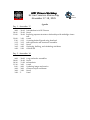
Agenda
Day 1 – November 17
9:00 – 10:45
10:45 – 11:00
11:00 - 12:00
12:00
1:30
2:15
3:15
3:45
4:30
-
1:30
2:15
3:15
3:45
4:30
5:30
Introduction to UCSF Chimera
Break
Exploring sequence-structure relationships with MultAlign viewer
tool
Lunch
Screening docked ligands using ViewDock
MD trajectories and structural ensembles
Break
Displaying, defining, and calculating attributes
General lab
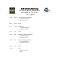
Day 2 – November 18
9:00
10:00
10:30
11:30
1:00
2:00
3:00
3:30
– 10:00
– 10:30
- 11:30
- 1:00
- 2:00
- 3:00
- 3:30
- ??
Large molecular assemblies
Break
Volume data
Lunch
Producing images and movies
Chimera scripts and demos
Break
Panel
UCSF Chimera Workshop
UC San Francisco
November 17-18, 2005
UCSF
Chimera
Day 1 Agenda
9:00 – 10:45
Introduction to UCSF Chimera
• Welcome & overview
• Introductory tutorial
• Hands-on session
10:45 – 11:00
Break
11:00 - 12:00
Exploring sequence-structure relationships with MultAlign viewer
tool
Presentation/Demo
Hands-on session
12:00 - 1:30
Lunch
1:30 - 2:15
Screening docked ligands using ViewDock
Presentation/Demo
Hands-on session
2:15 - 3:15
MD trajectories and structural ensembles
Presentation/Demo
Hands-on session
3:15 - 3:45
Break
3:45 - 4:30
Displaying, defining, and calculating attributes
Presentation/Demo
Hands-on session
4:30 - 5:30
General lab
• Get help working with data of your choice
UCSF Chimera Workshop
UC San Francisco Mission Bay
November 17-18, 2005
Day 2 Agenda
9:00 – 10:00
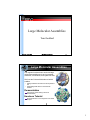
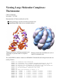
Large molecular assemblies
• Presentation/Demo
• Hands-on session
10:00 – 10:30
Break
10:30 - 11:30
Volume data
Presentation/Demo
Hands-on session
11:30 - 1:00
Lunch
1:00 - 2:00
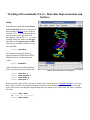
Producing images and movies
Presentation/Demo
Hands-on session
2:00 - 3:00
Chimera scripts and demos
Presentation/Demo
Hands-on session
3:00 - 3:30
Break
3:30 - ??
Panel
Chimera Futures
Q&A
UCSF
Chimera
UCSF Chimera Workshop, Fall
2005
Conrad Huang
UCSF
Resource for Biocomputing, Visualization, and
Informatics
University of California at San Francisco
November 17 & 18,
2005
1
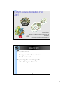
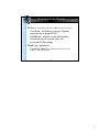
Overview
• General format:
– Short presentation/demonstration
– Hands-on tutorial
• Topics may be domain-specific
– Attend the topics of interest
2
1
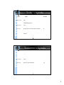
Today’s Agenda
Time
Presenter
Topic
Eric
9:00-10:45
Introduction to UCSF Chimera
10:45-11:00
Break
11:00-12:00
Exploring sequence-structure relationships
with MultAlignViewer
12:00-1:30
Lunch
1:30-2:15
Screening docked ligands using ViewDock
Elaine
2:15-3:15
MD Trajectories and structural ensembles
Eric
3:15-3:45
Break
3:45-4:30
Displaying, defining and calculating
attributes
Conrad
4:30-5:30
General lab
Team
Elaine
3
Tomorrow’s Agenda
Time
Presenter
Topic
Tom
9:00-10:00
Large molecular assemblies
10:00-10:30
Break
10:30-11:30
Volume data
11:30-1:00
Lunch
1:00-2:00
Producing images and movies
Greg
2:00-3:00
Chimera scripts and demos
Greg
3:00-3:30
Break
3:30-??
Tom
Team
Panel discussion
4
2
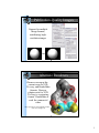
Today’s Presenters
•
•
•
•
•
•
Conrad Huang
Eric Pettersen
Elaine Meng
Tom Goddard
Greg Couch
Scooter Morris
Chimera Developer
Chimera Developer
Scientific Advisor
Chimera Developer
Chimera Developer
Executive Director, RBVI
5
Acknowledgements
• Staff:
– Dr. Tom Ferrin, Dr. Conrad
Huang, Tom Goddard, Greg
Couch, Eric Pettersen, Dan
Greenblatt, Al Conde, Dr.
Elaine Meng, Dr. John
“Scooter” Morris
• Collaborators (partial list):
Funding:
–NIH National Center for
Research Resources
–grant P41-RR01081
Further information:
–www.cgl.ucsf.edu/chimera
6
– Patricia Babbitt, UCSF
– Wah Chiu and Steven
Ludtke, Baylor
– John Sedat and David
Agard, UCSF
– David Konerding and
Steven Brenner, UCB
3
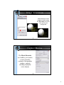
Chimera: the basics plus a few tips
• A whirlwind tour of the basics
– With focus on a few things to make your life
easier
• Hands-on experience
– “Getting started” tutorial
• Fleshes out the basics for those who haven’t used
Chimera before — and a good refresher for others
1
1
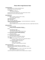
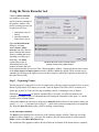
Chimera Basic Usage Reminder Sheet
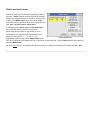
Open/Save Dialogs
drop-down menus for recently used files/directories
File Type filter controls type of files shown
multi-select by:
mouse drag (contiguous)
control click (non-contiguous)
Windows will have drive selection menu under leftmost browser column
double-click to choose one item and open/save it
Model Manipulation
left mouse:
rotate like grabbing trackball (center of screen)
Z axis rotation (edge of screen)
middle mouse translates
right mouse scales
Mac ➙ alt=middle, apple=right
"active" models respond to mouse motion -- controlled in Model Panel or command line
clip planes controlled with Side View tool
grab and drag with mouse
grab with middle button will move planes parallel (near plane) or together/apart (far plane)
Making Selections
Action/Selection paradigm
Actions menu works on whatever is selected
if nothing is selected, Actions work on everything
Mouse
control-left click to select
control-left drag to region select
control-shift-left click/drag to toggle selection status
control-click on nothing to deselect everything
up arrow increases selection to residue/chain/molecule
down arrow reverses
left arrow undoes last selection change
shift left arrow clears selection
right arrow inverts selection (in models with selections)
shift right arrow inverts selection in all models
Select menu
change Selection Mode to compose more complicated selections
remember to change back when done!
selections can be named so that they are:
saved in sessions
usable in typed commands
retrievable from Named Selections submenu
Working with Selections
Actions menu allows coloring, labeling, etc. of selections
Focus action centers selection in view and makes it center of rotation
Selection Inspector
invoked from Actions menu or button at bottom right of main window
shows details of items
allows modification of selected items' attributes
contents of selection can be written to a file from Actions menu or inspector
Color Wells/Color Editor
gray squares with sunken square centers are color wells
color wells control the color of an item
clicking on a color well with bring up the color editor
Color Editor
has red/green/blue sliders for controlling color
color names that Chimera knows can be typed into text area
where appropriate, an Opacity button brings up an opacity slider
opacity controls transparency (inversely)
No Color button (if present) unsets the items color
colors can be dragged and dropped between wells or from editor to well
Tool Shortcuts
tools can be put in the Favorites menu or on a toolbar for quick access
use Favorites...Add to Favorites/Toobar... menu item
remember to use Save button to preserve your changes
Command Line
up arrow retrieves previous command (down arrow the reverse)
buttons control "activity" (response to mousing) of models
Problems/Questions
full documentation in Help Menu (User's Guide)
search documentation with Help...Search Documentation
use Help menu's Report A Bug/Contact Us items to report problems/ask questions
Distances/Torsions
tool in Structure Analysis category
select two atoms or one bond
shortcuts to set up distance/torsion:
distance
select one atom
select second atom (control left shift) but with double click
choose Show Distance from popup context menu
torsion
select bond but with double click
choose Rotate Bond from popup context menu
Sequence
sequences can be viewed/searched with Tools...Structure Analysis...Sequence
Hydrogen Bonds
use FIndHBond tool in Structure Analysis category
creates pseudobonds between atoms to depict H-bonds
use Pseudobond Panel to fine tune depiction or remove the pseudobonds
~hbonds command will also remove H-bonds
Pseudobond Panel is in General Controls category
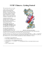
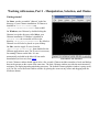
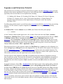
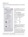
UCSF Chimera - Getting Started
This tutorial provides an overview
of basic features in Chimera for
displaying and manipulating
structures. You can interact with
Chimera by using the menus and/or
by entering commands. The basic
features of Chimera are available
either way, but several tools are not
available as commands, and several
command operations (and
scripting) are not available through
the menus. Thus, it is useful to
become familiar with both ways of
interacting with Chimera.
The Working with menus and
Working with commands sections
were designed to be independent of
each other. They cover (for the
most part) identical operations,
accomplished in different ways. If
you go through both sections, you
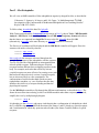
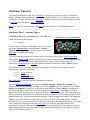
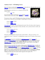
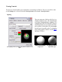
DNA helix with bound netropsin (6bna)
can skip portions that cover issues you already understand. You can also go back and forth between the
sections to see the correspondence between menu and command operations.
To follow the tutorial, you will need to access the Protein Data Bank (PDB) files 1zik and 6bna. If you have
Internet access, these can be fetched directly from the Protein Data Bank, as described below. If you do not
have Internet access, you can use the files included in the Chimera distribution. To do so,
1.
2.
3.
4.
start Chimera as described below
choose Help→Tutorials from the Chimera menu
click the link for either Getting Started tutorial
use the links to 1zik.pdb and 6bna.pdb to download the files to a convenient location on your
computer
5. carry on with the tutorial
Outline:
Working with menus - Part 1
Getting started
Opening a structure
Side View
Using the mouse
Selection/Action
Changing the display
Models and model status
Working with menus - Part 2
Setup
Representations and labels
Surfaces
Front image how-to (menu)
Working with commands - Part 1
Getting started
Opening a structure
Side View
Using the mouse
Command/Target
Changing the display
Models and model status
Working with commands - Part 2
Setup
Representations and labels
Surfaces
Front image how-to (commands)
Typographical Conventions
Item
Example
Description
Keyboard key
Ctrl
The control key
Mouse key
Btn1
Mouse button 1 (left button)
Menu action
File→Open
File Menu bar pulldown,
followed by Open
Filename (or file path) 1zik.pdb File 1zik.pdb
Working with menus, Part 1 - Manipulation, Selection, and Chains
Getting started
On Linux, run the executable "chimera" in the bin
directory of your Chimera installation. If Chimera is
installed in /usr/local/chimera, run
/usr/local/chimera/bin/chimera from a shell.
On Windows, start Chimera by doubleclicking the
Chimera icon in the directory called bin in your
Chimera installation. If Chimera is installed in
\Program Files the executable will be in the
directory \Program Files\Chimera\bin. By default, a
Chimera icon will also be placed on your desktop.
On Mac, start the Apple X server found in
/Applications/Utilities/X11, then doubleclick the
Chimera application to start. The X server is necessary
for running Chimera on the Mac. It is not
automatically included in the Mac OS, but can be
downloaded (as freeware) from Apple.
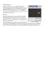
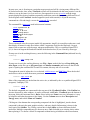
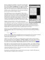
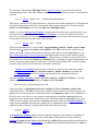
UCSF Chimera with 1zik loaded
A basic Chimera window should appear after a few seconds. Chimera includes a number of tools and dialogs
that can be present on the screen at the same time. The basic Chimera window provides the main interactive
workspace for displaying and manipulating structures. The default Chimera graphics window is pretty small,
so if you like, resize the main Chimera window by placing the cursor on any corner and dragging with the
left mouse button.
Opening a structure
Now open a structure. If 1zik.pdb was downloaded to your
machine, choose the menu item File→Open. Locate the file 1zik.pdb
in the resulting dialog and open it (the File type should be set to all
(guess type) or PDB). If you want to fetch directly from the PDB
instead, choose File→Fetch by ID and type 1zik in the PDB ID field.
The structure will appear in the main graphics window; it is a leucine
zipper formed by two peptides.
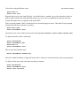
Side View
Scaling and clipping operations can be performed with the Side
View. There are several ways to start this tool; one is to choose
Tools→Viewing Controls→Side View from the menu. By default, the
Side View is also listed in the Favorites menu. The Side View shows a
tiny version of the structure.
Side View showing 1zik
Within the Side View, try moving the eye position (the small square;
scales the view) and the clipping plane positions (vertical lines) with the left mouse button. The Side View
will renormalize itself after movements, so that the eye or clipping plane positions may appear to "bounce
back" after you have adjusted them; however, your adjustments have been applied to the main display.
Using the mouse
Try manipulating the structure in the main
window with the mouse. By default, the left
mouse button controls rotation, the middle mouse
button controls XY translation, and the right
mouse button controls scaling. On a Mac with a
one-button mouse, the middle and right buttons
can be emulated by combining mouse action with
the option and
(apple) keys, respectively.
Default Mouse Button Assignments
Mouse button
Modifier
Action
Btn1
(left button)
Rotation
Btn2
(middle button)
XY Translation
Btn3
(right button)
Scaling
Btn1
Ctrl
Picking (selection)
Btn1
Ctrl-Shift
Addition to (removal from) selection
Continue moving and scaling the structures with
the mouse in the graphics window and Side View as desired throughout the tutorial.
In combination with the control (Ctrl) key, the mouse buttons have additional functions. By default, picking
from the screen (a type of selection) is done by clicking on the atom or bond of interest with the left mouse
button (Btn1) while holding down the Ctrl key. To add to an existing selection, also hold down the Shift key.
The selection is highlighted in green, and its contents are reported on the button near the lower right corner of
the graphics window.
You can also drag out a selection area with Ctrl-Btn1 (sweep out an area before releasing). All atoms and
bonds within that area will be selected. As before, Ctrl-Shift-Btn1 can be used to add to an existing selection,
either by clicking or by dragging.
The arrow keys can be used to broaden, narrow, or invert a selection. Chimera maintains a hierarchy of
objects from atoms to residues to chains to models. If an atom is selected, the ↑ key will broaden the selection
to the residue containing that atom. If an entire residue is selected, the ↑ key will broaden the selection to the
chain containing that residue. If a chain is selected, the ↑ key will broaden the selection to the entire model.
Similarly, the selection scope can be narrowed using the ↓ key. The → key inverts the selection so that
selected atoms become deselected and vice versa.
Spend some time selecting various parts of the model. An easy way to deselect everything is to use Ctrl-Btn1
in any blank space in the graphics window.
Selection/Action
Actions Menu Items
Menu Item
In general, operations performed with
the Chimera Actions menu affect the
current selection. Selections can be
made in many ways, including with the
Select menu or with the mouse (as
described above). When nothing is
selected, the Actions menu applies to
everything.
Description
Atoms/Bonds
Controls the display and representation of atoms and bonds.
Ribbon
Controls the display and representation of ribbons.
Surface
Controls the display and representation of molecular surfaces.
Color
Colors selected objects. Color target can be limited to object types
indicated by the radio buttons.
Label
Labels selected atoms. The residue submenu labels residues
containing the selected atoms.
Focus
Focuses the view on the selected atom(s), zooming and translating if
necessary.
Set Pivot
Sets the center of rotation based on the selected atom(s) without
adjusting the view.
Target
Restricts target of the action to certain selected or unselected object
types.
Changing the display
Inspect
Launches the Selection Inspector.
Write List
Writes a list of the currently selected objects to a parsable text file.
To simplify the display, use
Write PDB
Writes the coordinates of the currently selected atoms to a PDB file.
The current selection is highlighted in
green in the structure(s) and its
contents are reported on the button
near the lower right corner of the
graphics window.
Actions→Atoms/Bonds→hide to
undisplay the model followed by Actions→Atoms/Bonds→chain trace only to display only the chain trace. The
chain trace includes just the α-carbons (atoms named CA), connected in the same way that the residues are
connected.
Next, thicken the lines to make them more visible:
Actions→Atoms/Bonds→wire width→3
Try picking two α-carbons, one from each peptide (using Ctrl-Btn1 for the first, Ctrl-Shift-Btn1 for the second).
Label the atoms you have selected, first by atom name and then by residue name and number:
Actions→Label→name
Actions→Label→off
Actions→Label→residue→name + specifier
Each residue label is of the form:
res_name res_number.chain
It is now evident that one peptide is chain A, and the other is chain B. To deselect the atoms, pick in a region
of the graphics window away from any atoms or use the menu item Select→Clear Selection.
Undisplay the residue labels:
Actions→Label→residue→off
Color the two chains different colors:
1zik colored by element
Select→Chain→A
Actions→Color→cyan
Repeat the process to color chain B yellow. As described above, another way to select an entire chain is to
pick an atom or bond in the chain and then hit the ↑ key twice, once to expand the selection to the entire
residue and another time to expand it to the entire chain.
There is actually another "chain" in this model, not currently displayed: water. This chain ID was assigned
automatically when the structure was read in.
Select→Chain→water
Actions→Atoms/Bonds→show
Alternatively, the water could have been selected using Select→Structure→solvent or Select→Residue→HOH
To display all atoms of the A chain only:
Select→Clear Selection
Actions→Atoms/Bonds→hide
Select→Chain→A
Actions→Atoms/Bonds→show
Then to show the backbone only,
Actions→Atoms/Bonds→backbone only
Only the A chain's backbone is displayed because the A chain was selected when the action was performed.
To display all the atoms and color them according to element:
Select→Clear Selection
Actions→Atoms/Bonds→show
Actions→Color→by element
Models and model status
Generally, each file of coordinates opened in Chimera
becomes a model with an associated model ID number.
Models are assigned successive numbers, starting with
0 (zero). The Model Panel shows the current models
and enables many operations upon them. Open this tool
with Tools→General Controls→Model Panel.
A checkbox in the Active column of the Model Panel
shows that the model is activated for motion;
unchecking the box makes it impossible to move.
Checking the box again restores the movable state.
Make sure the line for 1zik.pdb (or 1zik) is
Chimera Model Panel
highlighted on the left side of the Model Panel (if not,
click on it) and then click close in the list of functions on the right side. Use the Close button at the bottom to
close the Model Panel.
Go on to Part 2 below, or terminate the Chimera session. A Chimera session may be ended using File→Quit.
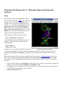
Working with Menus, Part 2 - Molecular Representations and
Surfaces
Setup
With Chimera started and the Side View opened as
described at the beginning of Part 1, open a different
structure. If 6bna.pdb was downloaded to your
machine, choose the menu item File→Open. Locate
the file 6bna.pdb in the resulting dialog and open it
(the File type should be set to all (guess type) or
PDB). If you want to fetch directly from the PDB
instead, choose File→Fetch by ID and type 6bna in the
PDB ID field. The structure contains the molecule
netropsin bound to double-helical DNA.
Thicken the lines to make them more visible:
Actions→Atoms/Bonds→wire width→3
Color the different nucleotides different colors. For
example, color the adenosine residues (adenine
nucleotides) blue:
Select→Residue→A
Actions→Color→blue
Chimera showing ball & stick (6bna)
Analogously, color cytosine nucleotides (C residues)
cyan, guanine nucleotides (G residues) yellow, and thymine nucleotides (T residues) magenta. Clear the
selection by using Select→Clear Selection or picking in a region of the graphics window away from any
atoms.
Rotate, translate, and scale the structure as needed to get a better look (see Using the mouse to review how
this is done). Continue moving and scaling the structure as desired throughout the tutorial. There are still
many white atoms, including the netropsin molecule in the minor groove of the DNA and water. Undisplay
the water:
1. pick one of the white dots with Ctrl-Btn1 (the white dots are water oxygens; if you cannot see them, first
change to a stick representation with Actions→Atoms/Bonds→stick)
2. hit the ↑ key once to expand the selection to the entire "chain" water; only one click is needed because
the picked atom is equivalent to an entire residue
3. Actions→Atoms/Bonds→hide
Representations and labels
Before proceeding, clear the selection. Otherwise, the
water will remain selected, potentially causing
confusion when menu Actions have no visible affect
(they affect only the selection, currently the invisible
waters).
Select→Clear Selection
Now that nothing is selected, the Actions menu will
Ribbon: flat, edged, and round
affect everything. Try some different molecular
representations. They can be translated, rotated, and scaled interactively. Multiple representation types can be
combined with each other and with surfaces (more on surfaces below).
Actions→Ribbon→show
Actions→Ribbon→round
Actions→Ribbon→hide
Actions→Atoms/Bonds→stick
Actions→Atoms/Bonds→sphere
Change the representation of only one of the DNA
strands, chain B:
Select→Chain→B
Actions→Atoms/Bonds→stick
Select→Clear Selection
Atoms/Bonds: wire, stick, ball & stick, and sphere
Next, change everything to a ball-and-stick representation:
Actions→Atoms/Bonds→ball & stick
In this representation, pick one of the atoms in the white netropsin molecule. Label the residue,
Actions→Label→residue→name + specifier
showing that it is named NT and is part of chain het (assigned automatically when the structure was read in).
The residue label might not be near the selected atom. Remove the residue label:
Actions→Label→residue→off
The first submenu under Label controls individual atom labels, while the second controls residue labels.
Actions→Label→name would have shown the name of the atom instead of the name of the residue.
Two white atoms that are not part of netropsin are displayed. They are apparently attached to cytosines,
which were previously colored cyan. Pick the two atoms and label their residues,
Actions→Label→residue→name + specifier
showing that one DNA strand is chain A, the other strand is chain B, and each strand contains a brominated
cytosine. Use Select→Clear Selection to deselect the atoms, then undisplay the residue labels:
Actions→Label→residue→off
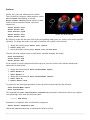
Surfaces
Finally, have some fun with molecular surfaces.
There are built-in categories within structures such as
main and ligand; when nothing is selected,
Actions→Surface→show displays the surface of main.
Surfaces can be translated, rotated, and scaled
interactively.
Actions→Surface→show
Actions→Surface→hide
Select→Structure→ligand
Actions→Surface→show
Actions→Surface→mesh
Surface: dot, mesh, and solid
By default, a surface has the same color as the corresponding atoms; however, surface color can be specified
separately. To change the surface color only of netropsin only (which is still selected):
1. change the coloring target: Actions→Color→surfaces
2. Actions→Color→red
3. restore the default coloring target: Actions→Color→all of the above
Clear the selection, change back to a solid surface, and then undisplay the surface.
Select→Clear Selection
Actions→Surface→solid
Actions→Surface→hide
As an example of a more complicated selection process, show the surface of the adenine and thymine
nucleotides in chain B only:
1. change the selection mode: Select→Selection Mode→append
2. Select→Residue→A
3. Select→Residue→T
4. change the selection mode: Select→Selection Mode→intersect
5. Select→Chain→B
6. Actions→Surface→show
To prepare for any subsequent operations, restore the selection mode and clear the selection:
Select→Selection Mode→replace
Select→Clear Selection
The command line (Tools→General Controls→Command Line) equivalent is much more concise, but requires
some knowledge of the atom specification syntax:
Command: surf :a.b,t.b
Sometimes it is helpful to make a solid surface transparent:
Actions→Surface→transparency→50%
Choose File→Quit from the menu to terminate the Chimera session.
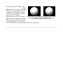
Front image how-to (menu)
Here are the steps to recreate the image at the front of the tutorial:
1. Read in 6bna.pdb (or fetch 6bna)
2. Set the representation to "stick":
Actions→Atoms/Bonds→stick
3. Undisplay the waters:
Select→Chain→water
Actions→Atoms/Bonds→hide
4. Color the residues:
Select→Residue→A
Actions→Color→blue
Select→Residue→C
Actions→Color→cyan
Select→Residue→G
Actions→Color→yellow
Select→Residue→T
Actions→Color→magenta
Select→Clear Selection
DNA helix with bound netropsin (6bna)
5. Add a surface to the DNA, color the surface light gray, and make surfaces transparent:
Actions→Surface→show
Actions→Color→surfaces
Actions→Color→light gray
Actions→Surface→transparency→50%
6. Add a surface to netropsin, color the surface red (it will already be transparent):
Select→Structure→ligand
Actions→Surface→Show
Actions→Color→red
Select→Clear Selection
7. Rotate and translate as desired
8. Change the background to white:
Actions→Color→background
Actions→Color→white
Actions→Color→all of the above
9. Save the image:
File→Save Image
Working with commands, Part 1 - Manipulation, Selection, and
Chains
Getting started
On Linux, run the executable "chimera" in the
bin directory of your Chimera installation. If
Chimera is installed in /usr/local/chimera,
run /usr/local/chimera/bin/chimera from
a shell.
On Windows, start Chimera by doubleclicking
the Chimera icon in the directory called bin in
your Chimera installation. If Chimera is
installed in \Program Files the executable
will be in the directory \Program
Files\Chimera\bin. By default, a Chimera
icon will also be placed on your desktop.
On Mac, start the Apple X server found in
/Applications/Utilities/X11, then
doubleclick the Chimera application to start.
The X server is necessary for running Chimera
on the Mac. It is not automatically included in
the Mac OS, but can be downloaded (as
freeware) from Apple.
Show the Command Line with Tools→General
Controls→Command Line. By default, the
Command Line tool is also listed in the
Favorites menu.
Chimera with Command Line and Side View
Opening a structure
A local file can be opened from the command line if it is in the working directory (or if the entire pathname is
entered):
Command: open 1zik.pdb
If the file has been downloaded but is not in the working directory, use File→Open instead, as described in
Part 2.
Alternatively, to fetch directly from the PDB, use the command:
Command: open 1zik
The structure will appear in the main graphics window; it is a leucine zipper formed by two peptides.
Side View
Scaling and clipping operations can be performed with the Side View. There are several ways to start this
tool; one is to choose Tools→Viewing Controls→Side View from the menu. By default, the Side View is also
listed in the Favorites menu. The Side View shows a tiny version of the structure.
Within the Side View, try moving the eye position (the small square; scales the view) and the clipping plane
positions (vertical lines) with the left mouse button. The Side View will renormalize itself after movements,
so that the eye or clipping plane positions may appear to "bounce back" after you have adjusted them;
however, your adjustments have been applied to the main display.
Using the mouse
1zik with tyrosine 17 (B chain) selected
Try manipulating the structure in the main window with the mouse. By default, the left mouse button (Btn1)
controls rotation, the middle mouse button (Btn2) button controls XY translation, and the right mouse button
(Btn3) controls scaling. On a Mac with a one-button mouse, the middle and right buttons can be emulated by
combining mouse action with the option and
(apple) keys, respectively.
Continue moving and scaling the structures with the mouse in the graphics window and Side View as desired
throughout the tutorial.
In combination with the control (Ctrl) key, the mouse buttons have additional functions. By default, picking
from the screen (a type of selection) is done by clicking on the atom or bond of interest with the left mouse
button (Btn1) while holding down the Ctrl key. To add to an existing selection, also hold down the Shift key.
The selection is highlighted in green, and its contents are reported on the button near the lower right corner of
the graphics window.
The arrow keys can be used to broaden (↑), narrow (↓), or invert (→) a selection. The hierarchy for
broadening and narrowing selections contains atoms, residues, chains, and models, in that order. When a
selection is inverted, the selected atoms become deselected and vice versa.
Spend some time selecting various parts of the model. An easy way to deselect everything is to use Ctrl-Btn1
in any blank space in the graphics window.
Command/Target
A Chimera command may include
arguments and a target (or atom
specification). For example, in the following
color command,
Command: color hot pink :lys
hot pink is an argument that specifies a
color name, and the target :lys specifies all
residues named LYS. (To see the built-in
colors and their names, choose
Actions→Color→all colors from the menu.)
If no target is specified, the command acts
on all applicable items. For example,
Atom Specification Symbols
Symbol
model number
# model (integer)
:
residue
: residue (name or number)
:.
chain ID
:.chain
@
atom name
@atom
*
whole wildcard
matches whole atom or residue names,
e.g., :*@CA specifies the α-carbons of
all residues
=
partial wildcard
matches partial atom or ressidue
names, e.g., @C= specifies all atoms
with names beginning with C
?
single-character wildcard used for atom and residue names only,
e.g., :G?? selects all residues with
three-letter names beginning with G
z<
zone specifier
or zr<zone spcifies all residues
within zone angstroms of the indicated
atoms, and za<zone specifies all atoms
(rather than entire residues) within
zone angstromgs of the indicated
atoms. Using > instead of < gives the
complement.
&
intersection
intersection of specified sets
|
union
union of specified sets
~
negation
negation of specified set (when
space-delimited)
would color all atoms, bonds, ribbons, and
molecular surfaces hot pink.
The command help can be used to show the
manual page for any command. For
example,
Usage
#
Command: color hot pink
Unlike the Actions menu, commands do not
automatically act on the current selection.
However, the current selection can be
specified as the target of a command with
the word selected, sel, or picked.
Function
z<zone
Command: help color
shows the manual page for the command color. The Chimera Quick Reference Guide lists all of the
commands and gives some examples of atom specification. It can be accessed by choosing Help→Tutorials
from the Chimera menu and clicking the "Chimera Quick Reference Guide" link.
Changing the display
To simplify the display:
Command: chain @ca
This command shows only the atoms named CA (α-carbons) and connects them in the same way that the
residues are connected. Next, thicken the lines:
Command: linewidth 3
Try picking two α-carbons, one from each peptide (using Ctrl-Btn1 for the first, Ctrl-Shift-Btn1 for the second).
Label the atoms you have selected:
Command: label sel
The label command shows atom information (atom name, by default). Undisplay the atom labels, then show
labels for the residues containing the selected atoms:
Command: ~label
Command: rlabel sel
Each residue label is of the form:
res_name res_number.chain
It is now evident that one peptide is chain A, and the other is chain B. To deselect the atoms, pick in a region
of the graphics window away from any atoms or use the menu item Select→Clear Selection. Undisplay the
residue labels:
Command: ~rlabel
Color the two chains different colors:
Command: color cyan :.a
Command: color yellow :.b
There is actually another "chain" in this model, not currently displayed: water. This chain ID was assigned
automatically when the structure was read in.
Command: disp :.water
displays the water (only the oxygens are visible in the X-ray structure);
Command: show :.a
gets rid of everything except the A chain, but displays all of its atoms;
Command: chain :.a@n,ca,c
shows the backbone of the A chain only. If the chain specification ":.a" had been omitted, then the backbones
of both chains would have been displayed.
Command: disp
Command: color byelement
displays all the atoms and colors them according to element.
Models and model status
Generally, each file of coordinates opened in Chimera becomes a model with an associated model ID
number. Models are assigned successive numbers, starting with 0 (zero). The Active models line in the
Command Line tool shows which models are activated for motion. The checkbox for 0 (currently the leucine
zipper) is activated. Unchecking the box makes it impossible to move model 0. Checking the box again
restores the movable state.
Command: close 0
closes the model. Go on to Part 2 below, OR terminate the Chimera session. A Chimera session may be
ended using the following command:
Command: stop
Working with commands, Part 2 - Molecular Representations and
Surfaces
Setup
With Chimera started and the Command
Line and Side View opened as described at
the beginning of Part 1, open a different
structure. If 6bna.pdb was downloaded to
your machine, choose the menu item
File→Open. Locate the file 6bna.pdb in the
resulting dialog and open it (the File type
should be set to all (guess type) or PDB).
Alternatively, fetch the structure directly
from the PDB:
Command: open 6bna
The structure contains the molecule
netropsin bound to double-helical DNA.
Thicken the lines to make them more
visible:
Command: linewidth 3
Color the different nucleotides different
colors, specifying them by residue name:
Command:
Command:
Command:
Command:
Chimera with Command Line, showing 6bna
color blue :a
color magenta :t
color yellow :g
color cyan :c
Rotate, translate, and scale the structure as needed to get a better look (see Using the mouse to review how
this is done). Continue moving and scaling the structure as desired throughout the tutorial. There are still
many white atoms, including the netropsin molecule in the minor groove of the DNA and water. Undisplay
the water:
Command: ~disp :.water
-OR- (these are equivalent)
Command: ~disp solvent
Representations and labels
Next, try some different molecular representations. They can be translated, rotated, and scaled interactively.
Multiple representation types can be combined with each other and with surfaces (more on surfaces below).
Command:
Command:
Command:
Command:
Command:
Command:
ribbon
ribrepr round
~ribbon
represent stick
repr sphere
rep stick :.b
The latter command changes only chain B to the stick representation, with the rest remaining in the sphere
representation.
Note that commands (but not their keyword arguments) can be truncated to unique identifiers. For example,
the command represent can be shortened to repr or rep but not re (because other commands also start with
re), whereas the keywords stick, sphere, etc. cannot be truncated.
Next, change everything to a ball-and-stick representation:
Command: repr bs
In this representation, pick one of the atoms in the white netropsin molecule. Label the residue,
Command: rlabel picked
showing that it is named NT and is part of chain het (assigned automatically when the structure was read in).
The residue label might not be near the selected atom. Remove the residue label:
Command: ~rlabel
Two white atoms that are not part of netropsin are displayed. They are apparently attached to cytosines,
which were previously colored cyan. Pick the two atoms and label their residues,
Command: rla picked
showing that one DNA strand is chain A, the other strand is chain B, and each strand contains a brominated
cytosine. Use Select→Clear Selection to deselect the atoms, then undisplay the residue labels:
Command: ~rla
Surfaces
Finally, have some fun with molecular
surfaces. There are built-in categories
within structures such as main and ligand;
when nothing is specified, surface shows
the surface of main. Surfaces can be
translated, rotated, and scaled
interactively.
Command: surface
Command: ~surface
Command: surface ligand
-OR- (these are
equivalent)
Command: surface :nt
-ORCommand: surface :.het
By default, a surface has the same color as
the corresponding atoms; however, surface
color can be specified separately:
Command:
Command:
Command:
Command:
Command:
Command:
Command:
surfrepr mesh
color red,s ligand
surfrepr solid
~surf
surf :a.b,t.b
surf :a,t
color green,s :t
Chimera showing a transparent surface (6bna)
Sometimes it is helpful to make a solid surface transparent. One way to do this is to define a transparent color
and then use the new color in a command:
Command: colordef tpink 1. .5 .7 .4
Command: color tpink,s
The numbers in the colordef command refer to red, green, blue, and opacity components, respectively.
Use the command stop to terminate the Chimera session.
Front image how-to (commands)
Here are the steps to recreate the image at the front of the tutorial:
1. Fetch 6bna:
Command: open 6bna
2. Set the representation to "stick":
Command: repr stick
3. Undisplay the waters:
Command: ~disp solvent
4. Color the residues:
Command: color blue :a
Command: color cyan :c
Command: color yellow :g
Command: color magenta :t
5. Add a surface to the DNA, color the surface transparent light gray:
Command: surf
Command: colordef tgray .827 .827 .827 .5
Command: color tgray,s
6. Add a surface to netropsin, color the surface transparent red:
Command: surf ligand
Command: colordef tred 1 0 0 .5
Command: color tred,s ligand
7. Rotate and translate as desired
8. Change the background to white:
Command: set bg_color white
9. Save the image:
Command: copy png file ~/Desktop/myfile.png
DNA helix with bound netropsin (6bna)
Exploring sequence-structure relationships
• Demo of selected tools in the Structure Comparison category
– Multalign Viewer - sequence alignment viewer with
many features, including crosstalk to and from
associated structures
– MatchMaker - constructs pairwise sequence alignments
and matches structures accordingly (demo: 1jta, 1bn8, 2pec)
– Match -> Align - constructs pairwise or multiple
sequence alignments based on pre-existing structural
superpositions
• Hands-on experience
– Sequences and Structures tutorial (the online version can be
accessed from the Chimera Help menu)
1
1
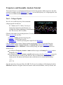
Sequences and Structures Tutorial
This tutorial focuses on looking at sequences and structures together using the Multalign Viewer extension.
Members of the enolase superfamily of enzymes are used to illustrate these features of Chimera. The enolase
superfamily has been described in several publications, including:
P.C. Babbitt, M.S. Hasson, J.E. Wedekind, D.R. Palmer, W.C. Barrett, G.H. Reed, I. Rayment,
D. Ringe, G.L. Kenyon, and J.A. Gerlt, "The Enolase Superfamily: A General Strategy for
Enzyme-Catalyzed Abstraction of the Alpha-Protons of Carboxylic Acids" Biochemistry
35:16489 (1996).
To follow along with the tutorial, you will first need to download the MSF file super8.msf into your working
directory. This file contains a sequence alignment of the barrel domains of eight enolase superfamily
members.
On Windows/Mac, click the chimera icon; on UNIX, start Chimera from the system prompt:
unix: chimera
A basic Chimera window should appear after a few seconds. Choose the menu item Tools... Structure
Comparison... Multalign Viewer. In the resulting dialog, locate and open super8.msf (the file type is MSF).
A Multalign Viewer window containing the alignment will appear. Multalign Viewer has its own
preferences; choose Preferences... Layout from the Multalign Viewer menu and change the font size and
the sequence-wrapping behavior as desired. Size and place the sequence window and main Chimera window
so that both are visible. If the sequence window becomes obscured at any point, it can be raised from the
Chimera Tools menu (Tools... MAV - super8.msf... Raise).
When the mouse focus is in the sequence window, the Page Down key (or space) moves the alignment view
down and Page Up (or Shift-space) moves the alignment view up. The names of the sequences are shown on
the left; a Consensus sequence and Conservation histogram are shown above the multiple alignment. The
superfamily is very diverse; there are very few positions in the alignment in which all the sequences have the
same residue (indicated with a red capital letter in the consensus sequence).
The first sequence in the alignment, named mr, corresponds to the barrel domain of mandelate racemase
from Pseudomonas putida. The next-to-the last sequence in the alignment, named enolyeast, corresponds to
the barrel domain of enolase from Saccharomyces cerevisiae. There are multiple structures in the Protein
Data Bank for each of these sequences; 2mnr (mandelate racemase) and 4enl (enolase) are used in this
tutorial.
To open the structures, choose File... Fetch by ID from the Chimera menu. In the resulting dialog, check the
PDB ID option (if it is not already checked) and the option to Keep dialog up after Fetch. Enter 2mnr in
the blank marked PDB ID and click Fetch. Repeat the process to fetch 4enl, and then click Close to dismiss
the dialog. Chimera will attempt to find the files within a local installation of the Protein Data Bank. If a file
is not found locally, Chimera will try to retrieve it from the Protein Data Bank web site. If this procedure
does not work, it may be that you do not have internet connectivity; instead, download the files 2mnr.pdb and
4enl.pdb included with this tutorial and open them in that order as local files (with File... Open).
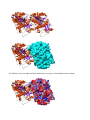
The view is initially centered on a protein colored white, the mandelate racemase structure. Off to the side
(and possibly out of view) is the enolase structure, which is colored magenta. Readjust the view to focus on
both structures:
Actions... Focus
The structures are not matched in any way; the coordinates are taken straight from the Protein Data Bank.
Rotate, translate, and scale the structures as needed to get a better look (see mouse manipulation to review
how this is done). If you like, open the Side View; choosing Tools...Viewing Controls... Side View is one
way to do this. Continue moving and scaling the structures as desired throughout the tutorial.
Notice that in the sequence window, the sequence names mr and enolyeast are now shown in bold within
boxes colored white and magenta, respectively. This means that the sequences have been compared with the
sequences in the structures, found to match sufficiently well, and automatically associated with the structures.
The colors indicate which sequence has been associated with which structure.
The alignment includes just the barrel domains, so it will be simplest to display only a chain trace of these
portions. First, open the Command Line; choosing Tools... General Controls... Command Line is one way
to do this. Next, find out which residue numbers in the structures correspond to the beginning and end of the
alignment. In general, these numbers will not be the same as the numbers marked on the alignment. However,
placing the cursor over any residue in a sequence that is associated with a structure gives the corresponding
structure residue number near the bottom of the sequence window. In each of the two structure-associated
sequences, find out the starting and ending residue numbers by placing the cursor over the first and last
residues in the alignment. Doing this reveals that the residue ranges are 134-317 in the mandelate racemase
structure and 151-400 in the enolase structure. Display the alpha-carbon chain traces of the barrel domains
and increase the linewidth (review atom specification syntax if desired):
Command: chain #0:134-317@ca
Command: chain #1:151-400@ca
Command: linewidth 2
The sequence alignment can be used to guide a structural match. From the Multalign Viewer menu, choose
Structure... Match... and make 2mnr the reference structure and 4enl the structure to match. Click Apply
without checking any boxes. This causes the match to use all pairs of alpha-carbons of residues aligned in the
sequence alignment. Readjust the view to focus on the structures:
Actions... Focus
The match is fairly rough; the RMSD is 8.4 angstroms (match values are written to the Reply Log, Tools...
Utilities... Reply Log). It is evident that not all of the residues aligned in the sequence alignment are really
structurally equivalent. Some loops in enolase (magenta) are much longer than those in mandelate racemase
(white). Try the structure matching again, but this time, check the box marked Iterate by pruning... and edit
the angstrom value to 1.0 before clicking OK. This will superimpose only the pairs that collectively match
very well in space. Visually, the match is improved; the dissimilar loops were not used in the match.
Next, we will see where some of the conserved residues are within the structures. In the sequence window,
use the mouse to drag a column containing the first completely conserved residue in the alignment (the
aspartate, D, at alignment position 99). This selects the residues in the associated structures, which then can
be displayed:
Actions... Atoms/Bonds... show
Open the Region Browser (Tools... Region Browser in the Multalign Viewer menu). If a sequence region
is created by mistake, it can be deleted by clicking on its line and then Delete within the Region Browser.
Create another region (this time, press Ctrl along with the mouse button to start a new region) for the next
completely conserved residue. This is a glutamate, E, at alignment position 148; display it too:
Actions... Atoms/Bonds... show
The displayed residues point into the center of the barrel, ligating a catalytically important metal ion. Display
the Mn++ ion in mandelate racemase:
Select... Chemistry... element... other... Md-Ni... Mn
Actions... Atoms/Bonds... show
Actions... Atoms/Bonds... sphere
Actions... Color... yellow
Select... Clear Selection
Sequence regions can be created automatically. From the Multalign Viewer menu, choose Structure...
Secondary Structure... show actual. This creates regions in the structure-associated sequences named
structure helices and structure strands colored goldenrod and lime green, respectively (yes, these are really
named colors). The region names are listed in the Region Browser. Clicking on a region in the sequence
window (or clicking the Active checkbox for that region in the Region Browser) will select the
corresponding residues in any associated structures. For sequences not associated with structures,
Structure... Secondary Structure... show predicted creates regions named predicted helices and predicted
strands colored gold and light green, respectively. The GOR method is used for prediction. Close the
Region Browser if it is open.
A structure can be colored according to the conservation in an associated sequence alignment. First, close
one of the structures, clear any selections, and show a ribbon for the other structure:
Command: close 1
Command: ~select
Command: ribbon
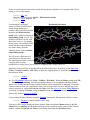
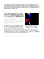
Choose Structure... Render by Conservation from the Multalign Viewer menu. The resulting Render by
Attribute tool shows a histogram of the residue attribute mavPercentConserved, the percent conservation
of the most prevalent residue at the corresponding position in the alignment. Adjust the coloring sliders on
the histogram (and their Color values, if desired) before clicking Apply. Coloring the structure by
mavPercentConserved shows the high conservation of the metal-binding residues and the low conservation
of most residues around the outside of the barrel.
The residue attribute mavConservation is also listed in the Render by Attribute dialog. Its values are those
shown in the Conservation line in the sequence window. Several different methods for calculating
conservation are available. The Multalign Viewer Analysis preferences (Preferences... Analysis) control
which method is used. If you wish, try using and visualizing different measures of conservation. After
changing any conservation parameters, it is necessary to Refresh... Histogram/List in the Render by
Attribute tool before clicking Apply. When finished, Close the Multalign Viewer preferences and Render
by Attribute.
See the Multalign Viewer documentation for a full description of its many functions, including alignment
editing. A number of sequence alignment formats can be read in and (with or without prior editing) written
out.
When finished, end the Chimera session:
Command: stop
Screening docked ligands
• Demo of selected tools in the Surface/Binding Analysis category
– ViewDock - facilitates screening of ligands
output by the program DOCK
– FindHBond - identifies hydrogen-bonding
interactions based on atom types and
geometrical relationships
• Hands-on experience
– ViewDock tutorial (the online version can be accessed
from the Chimera Help menu)
1
1
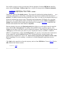
ViewDock Tutorial
The program DOCK calculates possible binding orientations, given the structures of ligand and
receptor molecules. The structure of a physiologically important target molecule can be used to find
other molecules that may bind it and modulate (usually inhibit) its function. Generally, one searches a
large database of commercially available compounds with DOCK, treating each as a possible
"ligand," against the structure of a target protein, treated as the "receptor." Simple scoring methods
are used to identify the most favorable binding modes of a given molecule, and then to rank the
molecules according to these best orientations. The output consists of a large number of candidate
ligands in the binding orientations considered most favorable by DOCK. It is then up to human users
to look through the molecules and decide which ones are worth pursuing in the real world. Please
consult the DOCK web site for more details.
ViewDock facilitates the selection of compounds by a human user from the output of DOCK
(versions 3, 3.5, the variant 3.5.x developed in the Shoichet laboratory, 4, and 5). In this tutorial, the
results of docking a small database of 30 compounds to the protein H-ras (from Protein Data Bank
entry 121P) are used to illustrate the workings of ViewDock. See the ViewDock manual page for a
more formal description of the program.
To follow along with the tutorial, you first need to download the files ras.pdb (the structure of the
receptor, H-ras), gto.pdb (the ligand GTO bound to H-ras in the original PDB file, for comparison
with docked molecules), ras.mol2 (the docked molecules output by DOCK 4, in Mol2 format), and
setup.com (a file containing commands that set up the viewing context) into your working directory.
On Windows/Mac, click the chimera icon; on UNIX, start Chimera from the system prompt:
unix: chimera
A basic Chimera window should appear after a few seconds. If you like, resize it by placing the cursor
on any corner and dragging with the left mouse button. Commands are entered into the Command
Line and scaling and clipping operations can be performed with the Side View. One of several ways
to start these tools is with Tools... General Controls... Command Line and Tools... Viewing
Controls... Side View in the menu. Tools can be moved to a convenient location on the screen by
dragging with the left or middle mouse button when the cursor is placed on the top bar.
First, open the (previously downloaded) structures of the receptor and its co-crystallized ligand.
Choose File... Open. In the resulting dialog, check the option to Keep dialog up after Open. Make
sure the File type is set to all (guess type) or PDB, then locate the files. Choose ras.pdb and click
Open; after that structure appears, open gto.pdb in the same way. Click Close to dismiss the dialog.
Next, start ViewDock (Tools... Surface/Binding Analysis... ViewDock); this brings up a dialog
requesting the file of docked ligands (also previously downloaded). Choose and open ras.mol2 (the
File type is Dock 4 or 5). The ViewDock ListBox will appear, along with a thicket of molecules in
the graphics window. Move the ListBox aside if it is obstructing the graphics window or any of the
other tools.
Now the receptor is in model 0, GTO is in model 1, and the docked molecules are in model 2 (the
lowest available model is used for each successive structure opened, and the file of docked molecules
was opened last).
In most cases, one is focusing on a particular target protein and will be viewing many different files
of docked molecules; thus, many ViewDock sessions will be initiated with the same protein. It can be
tedious to set up the same view over and over. One approach is to save a session with the target
protein displayed as desired, and then repeatedly restart that session before opening different files of
docked ligands with ViewDock. Another approach (used in this tutorial) is to put the necessary
commands in a file and simply execute the command file as needed.
The command file (setup.com) used in this tutorial contains:
color aquamarine #0
chain #0@ca
disp #0 & #2 z<5
color orange #0@o=
color medium blue #0@n=
repr bs #1
color magenta #1
color byatom #2
These commands color the receptor (model #0) aquamarine, simplify it to an alpha-carbon trace, and
then display all atoms for only the residues within 5 angstroms of any docked molecule. Oxygen
atoms in the receptor are colored orange, nitrogens medium blue. The co-crystallized ligand GTO
(#1) is shown in magenta ball-and-stick and the docked molecules (#2) are colored by atom type.
If setup.com is in the working directory, enter the following in the Command Line (indicated here by
Command:):
Command: open setup.com
If setup.com is not in the working directory, use File... Open, uncheck the box to Keep dialog up
after Open, set the file type to all (guess type) or Chimera commands, and browse to the file and
open it. Opening the command file executes its contents; this may take a few seconds.
Throughout the tutorial, adjust the view as desired with the mouse and Side View. Show the docked
molecules as sticks to make them more prominent:
Command: repr stick #2
Most of the compounds are docked into the active site, as indicated by the co-crystallized ligand GTO
(magenta). Undisplay GTO:
Command: ~disp #1
The docked compounds are enumerated in the top part of the ViewDock ListBox. If the ListBox has
become obscured by other windows, it can be resurrected with Tools... ViewDock (near the bottom of
the menu, below the horizontal line)... Raise. Since in this case Name is not very informative, it may
be helpful to add other descriptors to the listing. Use the Column menu to show Description and
Energy score, and to hide Name and Number.
Clicking on a line chooses the corresponding compound: the line is highlighted, just the chosen
compound is shown in the main graphics window, and more detailed information is shown in the
lower part of the ListBox. Try clicking various lines in the ListBox to choose different docked
molecules. Multiple compounds may be chosen at once. Ctrl-click adds to an existing choice rather
than replacing it. To choose a block of compounds without having to hold down the mouse button,
click on the first (or last) and then Shift-click on the last (or first) in the desired block.
The listing can be sorted by any column, by clicking on the header. Make sure the list is sorted by
Energy score, with the most negative values (which are the most favorable) at the top. Scroll down to
the lowest line in the top panel of the ListBox and click on it to choose the worst-scoring molecule.
The following command can be used to locate this molecule if it is outside the view:
Command: window
This compound is not docked in the active site like the others, and its docking scores are zero.
There are three mutually exclusive states that can be assigned to docked compounds. Viable
compounds are interesting (or have not been looked at yet), Deleted compounds are less interesting
but may deserve another look, and Purged compounds are definitely not interesting. The S column
shows V, D, and P to indicate these states. Viable and deleted but not purged molecules are included
when File... Rewrite is used. Change the status of the worst-scoring molecule to purged by clicking
the Purged checkbox near the bottom of the ListBox. Note that its listing disappears; make it
reappear by checking the box next to List Purged in the Compounds menu.
Normally, a user will click on successive lines, examine the compounds in the binding site, and
change the status of less interesting compounds to deleted or purged. Compounds can also be chosen
by descriptor values and then changed in status collectively. Several sessions may be needed to
whittle the list down sufficiently.
As an example, choose compounds based on their hydrogen-bonding interactions with the receptor.
HBonds... Add Count to Entire Receptor will bring up the FindHBond tool; make sure the
inter-model mode is set and increase the Line width to 3 (the detected hydrogen bonds will be
shown as lines). Click OK. When the calculation is finished, new columns of descriptors will appear
in the ListBox. Again, individual compounds can be examined by clicking on their respective lines in
the ListBox. Use the Column menu to hide the descriptors HBond Ligand Atoms and HBond
Receptor Atoms (the numbers of ligand and receptor atoms, respectively, participating in the
detected ligand-receptor hydrogen bonds).
Compounds... Choose by Value opens an interface with several sections. Choose from Viable
compounds and uncheck the boxes next to Description and Energy score to collapse the
corresponding sections. In the HBonds (all) section, move the sliders to include 0-1 hydrogen bonds.
A message near the top of the Choose by Value dialog will report that 17 of the 29 viable compounds
meet the criteria. Click OK to choose the compounds and dismiss the dialog. The 17 viable
compounds with 0-1 hydrogen bonds to the receptor will be chosen in the ListBox and displayed in
the main Chimera window. Change these compounds to purged by clicking the Purged checkbox
near the bottom of the ListBox. Uncheck the box next to List Purged in the Compounds menu to
remove the purged compounds from the listing.
Finally, we will flip through the remaining listed compounds with the Movie feature. First, place a
surface on the binding site (receptor residues within 7 angstroms of GTO; this may take a minute):
Command: surf #0 & :gto z<7
The surface can be made transparent with Actions... Surface... transparency... 60% (in the main
Chimera menu). Movie... Play (back in the ListBox menu) flips through all of the listed compounds,
in the order in which they are listed, regardless of status. It is possible to change the view and move
the molecules around while the movie is playing. The movie will loop continuously through the list
until halted with Movie... Stop. The length of time each compound is shown can be controlled with
Movie... Options. If molecules are "unlisted" using the checkboxes in the Compounds menu, they
are not included in the movie; in addition, the order of display depends on how the molecules are
sorted. No matter how the molecules are sorted in the ListBox, however, they remain in the original
order (minus any purged compounds) in output files created with File... Rewrite. Once you have seen
enough, stop the movie and exit from Chimera.
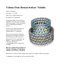
MD trajectories and structural ensembles
• MD Movie (this tool is in the MD/Ensemble Analysis category)
– Demo: trajectory playback/recording, holding
structural elements “steady”, RMSD
calculations, generation of occupancy maps
• Hands-on experience
– Trajectory and Ensemble Analysis tutorial (the
online version can be accessed from the Chimera Help menu)
1
1
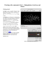
Trajectory and Ensemble Analysis Tutorial
This tutorial focuses on visualization and analysis of molecular dynamics (MD) trajectories and other
structural ensembles with the MD Movie tool. Part 1 uses an MD trajectory of a collagen peptide, and
Part 2 uses an NMR ensemble of Met-enkephalin.
Part 1 - Collagen Peptide
We will view an MD trajectory of the nonmutant
collagen peptide described in:
R. J. Radmer and T. E. Klein, "Severity of
Osteogenesis Imperfecta and Structure of a
Collagen-like Peptide Modeling a Lethal Mutation
Site" Biochemistry 43:5314 (2004).
(Thanks to the authors for providing the data!) To follow
along, download the data files:
leap.top - AMBER parameter/topology file
md01.crd - AMBER trajectory file
collagen.meta - metafile specifying these input files for MD Movie
Click the chimera icon; a basic Chimera window should appear after a few seconds. Show the
Command Line (Tools... General Controls... Command Line) and start MD Movie (Tools...
MD/Ensemble Analysis... MD Movie). In the resulting dialog, the inputs can be specified in two
different ways:
by setting the Trajectory format to Amber and browsing to the Prmtop file leap.top and the
Trajectory file md01.crd
by setting the Trajectory format to metafile and browsing to the file collagen.meta (it must be
in the same directory or folder as the other two files). It contains the following lines, which
simply specify the options and filenames that would otherwise be entered into the dialog:
amber
leap.top
md01.crd
Once the inputs have been specified, click OK. The first set of coordinates will be displayed and the
MD Movie controller will appear. Show the structure with sticks and ribbons, color by element, and
undisplay the hydrogens:
Command:
Command:
Command:
Command:
Command:
repr stick
ribbon
ribrepr smooth
col byelement
~disp H
Move and scale the structure as
desired throughout the tutorial. The
structure contains three chains.
Each chain is in a left-handed
polyproline II helix conformation, and together the chains form the right-handed triple helix
characteristic of fibrillar collagen. The ribbons are narrow because the peptides are not in a standard
alpha-helical conformation.
MD Movie
controller buttons Use the MD Movie controller to play the trajectory. From left to right, the
buttons mean: play backward continuously; go back one step; stop; go forward
one step; and play forward continuously. The rate of continuous play can be
adjusted with the Playback speed slider. The Frame number is reported and
can also be entered directly to view a specific frame. Frame number and Step size changes take
effect when return (Enter) is pressed. If the controller becomes obscured by other windows, it can be
raised using its instance in the Tools menu (near the bottom of the menu, below the horizontal line).
Show the sequence with Tools... Structure Analysis... Sequence. Fibrillar collagen typically
contains many -Gly-X-Y- repeats, where X is often Pro (proline) and Y is often Hyp
(hydroxyproline). Both Pro and Hyp are shown as P in the sequence panel. Mousing over the
sequences shows that the residues in the peptides are numbered 1-34, 35-68, and 69-102, respectively.
Selecting residues highlights both the sequences and the structures:
Command: sel :gly
Command: sel :pro
Command: sel :hyp
Close the sequence panel.
It may be useful to hold certain atoms steady during trajectory playback. For example, hold Glu-86
steady to view its interactions:
Command: sel :86
(from the controller menu) Actions... Hold selection steady
Command: color magenta sel
Command: ~sel
Even though it is no longer
selected, residue 86 will be held
steady during playback (as
possible; there will still be internal
motions) until Hold selection
steady with a different selection or
Stop holding steady is used. The
structure can still be moved with
the mouse, however. Try playing
the trajectory with residue 86 held
steady and then without holding
any atoms steady (from the
controller menu, choose Actions...
Stop holding steady).
Residue 86 held steady
We will create a short movie of
several frames in the trajectory.
The following procedure is just one
example; there are many
possibilities of what to show, how to show it, whether to use a script, and so on.
Adjust the Chimera window to the dimensions desired for the movie. If needed, use the Side View
(Tools... Viewing Controls... Side View) to adjust the clipping planes. Turn off the ribbon to reveal
the backbone atoms:
Command: ~ribbon
Use 2D Labels to add a title (Tools... Utilities... 2D Labels). When the Mouse setting in the 2D
Labels dialog is labeling, the left mouse button (button 1) is reassigned to labeling: clicking
starts a new 2D label and previously created 2D labels can be repositioned by dragging. Click in the
Chimera window where you would like to start a title and type in the title text; drag the text if you
want to reposition it. Adjust the Font size and Color (click the color well, use the Color Editor) to
your liking. Changing the Mouse setting to normal returns the left mouse button to its previous
function (by default, rotation of models).
Create another 2D label, this time using the 2dlabels command so that the label will have a name:
Command: 2dlabels create mylabel text temp
This label will be used to display the frame number. Make sure that the Mouse setting in the 2D
Labels dialog is labeling, then drag the temporary text to near the lower left corner of the Chimera
window. Adjust its Font size and Color to your liking, then Close the 2D Labels dialog.
Next, define a script to execute at each frame. Halt any playback. From the MD Movie controller
menu, choose Per-Frame... Define script. Enter a script to be interpreted as Chimera commands:
findhbond linewidth 2 color yellow
2dlabels change mylabel text "frame <FRAME>"
Uncheck the option to Use leading zeroes... This script will calculate the hydrogen bonds in
each frame, show them as yellow lines, and display the current frame number in the label named
mylabel. Click OK to dismiss the dialog with the script. Play a few steps by clicking the button to go
forward or backward one step at a time. The number and arrangement of H-bonds vary somewhat
from step to step. (Although the number of H-bonds cannot be accessed in Chimera commands, a
Python script could be used to display this information. For example, hbcount.py would show the
H-bond count instead of the frame number in mylabel.)
Halt any playback, but move the Playback speed slider all the way to the right. From the controller
menu, choose File... Record movie. If a dialog with an MPEG license agreement appears, click
Accept since the movie will not be used for commercial purposes. In the dialog for recording, choose
a File type you will be able to play back on your computer (the choices are MPEG-1, MPEG-2,
MPEG-4, and Quicktime). Change the Ending frame to 25, specify a convenient name and location
for the output file, and click Record. Frames 1-25 will then be played, saved as images, and
automatically assembled into a movie file. (Do not obscure any parts of the Chimera window while
this is occurring.) View the resulting 1-second movie with the appropriate application on your
computer.
Click Quit on the controller to close the trajectory and exit from MD Movie. Go on to Part 2 below,
OR terminate the Chimera session:
Command: stop
Part 2 - Met-Enkephalin
We will view an NMR ensemble of Met-enkephalin in negatively charged bicelles, as described in:
I. Marcotte, F. Separovic, M. Auger, and S. M. Gagne, "A Multidimensional 1H NMR
Investigation of the Conformation of Methionine-Enkephalin in Fast-Tumbling Bicelles"
Biophys J 86:1587 (2004).
To follow along, download the data file 1plx.pdb.
With Chimera started and the Command Line shown (as in Part 1), choose Tools... MD/Ensemble
Analysis... MD Movie. In the resulting dialog, choose PDB as the Trajectory format and indicate
that the frames are contained in a single file. Browse to the file 1plx.pdb, then click OK
(alternatively, a metafile in the same directory as 1plx.pdb could have been used).
The first set of coordinates will be displayed and the MD Movie controller will appear. Show the
structure with sticks colored by element:
Command: repr stick
Command: col byelement
Move and scale the structure as desired throughout the
tutorial. This structure is Met-enkephalin, with the sequence
Tyr-Gly-Gly-Phe-Met. Enkephalins are neuropeptides that
activate opioid receptors. Different subtypes of opioid
receptors mediate different but overlapping responses in the
body. For example, molecules that selectively activate
µ-opioid receptors are more effective for treating severe pain
than molecules that selectively activate δ-opioid receptors,
but are also more likely to cause constipation. The
conformations of molecules that bind opioid receptors
(enkephalins, morphine, etc.) are of interest because they
influence the selectivity of receptor binding and thus the
physiological response.
Use the MD Movie controller to flip through the different conformations, as described above. The
frames do not reflect time ordering, as this is an NMR ensemble rather than a trajectory. If desired,
simplify the view by undisplaying hydrogens:
Command: ~disp H
It is thought (see the reference and papers cited therein) that a conformation of enkephalin in which
the Tyr and Phe rings point in different directions (like frames 1 and 25) binds to µ-opioid receptors
and a conformation in which they point toward each other (like frames 2 and 80) binds to δ-opioid
receptors.
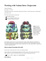
One way to analyze the ensemble is to calculate root-mean-square
deviations (RMSDs) between pairs of frames. From the controller
menu, choose Analysis... RMSD map. Click Apply on the RMSD
parameters dialog to perform the calculation without closing the
dialog. This will compute all pairwise RMSDs between frames and
show the result as a map in grayscale. After the initial calculation,
the map will be recolored to enhance contrast.
In the RMSD map, the axes are frame numbers; lighter squares
reflect pairs of frames with lower RMSDs (more similar structures)
and darker squares reflect pairs of frames with higher RMSDs (less
similar structures). Mousing over the map shows the RMSD values
and the numbers of the frames being compared. Clicking on the map
enters the corresponding pair of Frame numbers below the map.
Clicking Go then displays that frame in the main Chimera window.
Roughly, the upper left block of white in the map represents
conformations more similar to to a µ-binding conformation, and the
lower right block of white represents conformations more similar to a δ-binding conformation.
Similar conformations are mostly grouped together in this ensemble, but will not necessarily be
grouped together in ensembles in general. Also, ensembles usually contain many more groups of
conformations, especially for larger structures with more degrees of freedom.
All atoms were used in the RMSD calculation, because although the parameter Restrict map to
current selection, if any was set to true, nothing was selected. Select the nonhydrogen backbone
atoms only,
Command: sel @n,ca,c,o
and this time click OK to dismiss the RMSD parameters dialog and perform the calculation. Although
the two maps span different ranges in RMSD, they reveal essentially the same groups of
conformations. Close both maps.
Another way to analyze the ensemble is to calculate spatial occupancy maps for atoms of interest.
From the controller menu, choose Analysis... Calculate occupancy. The resulting dialog will show
the warning message "No atoms being held steady." This means you have not previously selected a
set of atoms and chosen Actions... Hold selection steady from the controller menu for this ensemble.
Why might it be useful to hold atoms steady while calculating occupancy? The contents of different
frames may move around enough to obscure certain spatial patterns. Even if the structure as a whole
is held fairly steady, one may want to hold a particular set of atoms (such as a sidechain) steady to
examine local interactions. However, if the structure or region of interest is already sufficiently
steady, the "hold steady" step can be omitted.
One approach to analyzing the relative positions of the aromatic rings is to hold the Phe ring atoms
steady and map the occupancy of the Tyr ring atoms:
1. Select the six Phe ring atoms. One way is to pick them from the screen (Ctrl-click on one,
Shift-Ctrl-click on each of the other five). Another way is with the command:
Command: sel :phe & aromatic ring
(the intersection of PHE residues with aromatic ring atoms)
2. Choose Actions... Hold selection steady from the controller menu.
3. Select the six Tyr ring atoms, by picking or with the command:
Command: sel :tyr & aromatic ring
4. If the occupancy dialog is not already up, choose Analysis... Calculate occupancy from the
controller menu.
5. Click OK on the occupancy dialog.
When the map has been computed, the Volume Viewer tool will
appear. This tool shows a histogram of the values in the map; the slider
controls what contour level is displayed.
Clear the selection in Chimera (Select... Clear Selection). In the
Volume Viewer tool, change from surface to mesh and move the
slider to a value of approximately 2. Use the Side View (Tools...
Viewing Controls... Side View) to move the clipping planes so that all
of the mesh is visible. Optionally, change the color of the mesh surface
by clicking the color well below the histogram and using the Color
Editor. (Volume Viewer is complex tool with many features. For
more on this tool, see the Volume Viewer manual page and the
Chimera tutorials on the web.)
You will see four main blobs or volumes representing probable
positions of the Tyr ring relative to the Phe ring (similar to the upper
image, which also shows frame 2). The two larger volumes represent
µ-type conformations and the two smaller volumes represent δ-type
conformations. The volume pairs are related by approximately 180-degree flips of the Phe ring.
Although the atom pairs CD1/CD2 and CE1/CE2 in the Phe ring are chemically equivalent, each
atom is distinguishable by name and is treated as distinct for holding steady.
If desired, flip through the ensemble (still holding the Phe ring steady) to verify that the volumes
show areas occupied by the Tyr ring. To delete the volume display, choose File... Close data from the
Volume Viewer menu.
Finally, calculate a map without holding any atoms steady. Choose Actions... Stop holding steady
from the controller menu. Since this ensemble maintains the Tyr ring in roughly the same place,
simply map the occupancy of the Phe ring atoms. Select the Phe ring atoms (as above), choose
Analysis... Calculate occupancy, and click OK. This time, the conformations are not as well
separated; two lobes of occupancy are apparent at a contour level of approximately 2 (similar to the
lower image, which also shows frame 2). One lobe represents µ-type conformations and the other
represents δ-type conformations.
When finished with the Met-enkephalin ensemble, quit from Chimera (File... Quit).
Displaying, Defining and
Calculating Attributes
Conrad Huang
November 17 & 18, 2005
UCSF Chimera Fall Workshop
1
Overview
• What are attributes?
• Depicting attributes graphically
• Selecting atoms, residues and molecules using
attribute values
• Using Chimera tools to add new attributes
• Defining your own attributes
2
1
What Are Attributes?
• Attributes are values associated with atoms, residues
and molecules
• Chimera knows a lot about some of them
– Atomic coordinates for graphical display
– Atom specifiers
• Chimera knows little about others
– Only name and value
– For example, PDB files include temperature factor and
occupancy for atoms
– Tools for manipulating these attributes can:
• depicting attributes graphically (e.g., by color)
• select atoms with chosen range of attribute values
3
Using Attributes
• Graphical interface
– Tools → Structure Analysis → Render by
Attribute
• Command line interface
– Atom specifier
• color blue @/bfactor > 50
• select @ca/bfactor < 50
– Command
• rangecolor bfactor 0 blue 50 yellow 75 red
– Both
• rangecolor bfactor 0 blue 50 yellow 75 red @ca
4
2
Render by Attribute
• Top section selects which
attributes to use
• Middle section sets action type
(changing graphical rendering
or selection) and parameters
• Bottom buttons apply the action
and/or closes the panel
5
Changing Graphical Rendering
• Change colors
– Select attribute to map
– Use histogram to select thresholds and associated
colors
• Control-click to add or remove thresholds
– Choose which colors (atoms, ribbons and/or
surfaces) to change
• “Keep opaque” discards transparencies in colors specified
in histogram
• If some atoms have no values for the selected attribute, a,
you can choose the default color for these atoms
– Click “Apply” to update display
6
3
Changing Graphical Rendering
• Changing atomic radii
– Select attribute to map
– Use histogram to select thresholds and associated
radius
• Control-click to add or remove thresholds
– Choose atom rendering style
• If some atoms have no values for the selected attribute, a,
you can choose whether radii of these atoms should
change, and (if yes) the default radius
– Click “Apply” to update display
7
Changing Graphical Rendering
• “Worms”
– Displaying ribbons whose size is a function of
attribute values
• Only works with residue attributes
– Use histogram to select thresholds and associated
radius
• Control-click to add or remove thresholds
– Choose ribbon rendering style
• Choose “non-worm” to go back to default ribbons
– Click “Apply” to update display
8
4
Changing Selection
• Click the “Select” tab
• Use histogram to set a minimum and a
maximum value
• Choose whether values between or outside the
extrema should be selected
• Click “Apply” to update selection
9
Adding Attributes
• Some attributes (e.g., temperature factor) are
read in as part of data files
• Chimera has tools that add attributes to open
models:
– MAV adds “mavPercentConserved” attribute
– “Tools → Surface/Binding Analysis → Surface
Area/Volume” adds surface area and volume
attributes using the NCBI StrucTools server
• Once created, these attributes can be
manipulated the same way as read-in attributes
10
5
Adding Your Attributes
• Attributes can be added
using a text file with
information on attribute
name and what objects
(atoms, residues or
models) are affected
• Atom specifiers are used
to assign values to
matching objects
# Assign atomic weights to atoms
attribute: aw
match mode: any
recipient: atoms
@/element="H"
1.00794
@/element="C"
12.0107
@/element="N"
14.0067
@/element="O"
15.9994
@/element="P"
30.973761
@/element="S"
32.06
11
Adding Your Attributes
• Graphical interface
– Tools → Structure Analysis → Define Attributes
• Command line interface
– defattr filename
– defattr filename spec atom_specifier
12
6
Calculating Attributes
• Attributes can be created by combining other
attributes using Tools → Structure Analysis →
Attribute Calculator
• Currently, only arithmetic operators, sum and
average are supported
13
Summary
• Chimera has tools for manipulating “generic”
attributes
– Tools are in category Structure Analysis
– Render by Attribute may be used to change
graphical rendering and to select atoms, residues and
models
– Define Attributes and Attribute Calculator may be
used to add new attributes
14
7
Attributes Tutorial
This tutorial demonstrates many uses of attributes, or properties of atoms, residues, and molecule
models. Attributes can be numerical (such as atomic number), boolean (e.g., whether a residue is an
alpha-helix), or string-valued (such as atom type). Attribute values can be rendered visually and used
in selection and command-line atom specification.
Part 1 uses a leucine zipper structure, and Part 2 uses the structure of a GTP-binding protein.
Attributes, Part 1 - Leucine Zipper
On Windows/Mac, click the chimera icon; on UNIX, start
Chimera from the system prompt:
1zik colored by accessibleSurface
unix: chimera
A basic Chimera window should appear after a few seconds.
Open the Command Line (choosing Tools... General
Controls... Command Line is one way) and, if desired, the
Side View for clipping and scaling.
If you have internet connectivity, structures can be obtained directly from the Protein Data Bank.
Choose File... Fetch by ID from the Chimera menu. In the resulting dialog, check the PDB ID option
(if it is not already checked) and fetch the PDB structure 1zik. If you do not have internet
connectivity, download the file 1zik.pdb included with this tutorial and use File... Open to open it.
The structure is a leucine zipper formed by two peptides. Undisplay water, change to a stick
representation, and color by element:
Command: ~disp solvent
Command: repr stick
Command: color byelement
Move and scale the structure as desired throughout the tutorial.
Open the Render by Attribute tool (Tools... Structure Analysis... Render by Attribute). It is
initially set to show the attributes of atoms. Look in the Attribute list to see the attributes available:
bfactor and occupancy, which were read from the input PDB file. Choose bfactor; a histogram of
the values will appear, with blue, white and red markers (or thresholds). Click Apply to color the
atoms blue to white to red in order of increasing B-factor. You can define your own color mapping by
adding and deleting thresholds (Ctrl-clicking an existing one deletes it; Ctrl-clicking elsewhere on the
histogram adds one), moving them along the histogram, and/or changing their colors. The Value and
Color are shown for the most recently clicked or moved threshold. The Value changes when the
threshold is moved, or the position can be changed by entering a value and pressing return. The Color
can be changed by clicking the adjacent color well. If you wish, try applying different color
mappings. As expected, the atoms with higher B-factors are on the outside of the structure. Note that
the histogram includes the B-factor values of the waters even though they are not displayed. Display
waters with B-factors less than 75:
Command: disp solvent & @/bfactor<75
Next, change to the attributes of residues in the Render by Attribute dialog. The automatically
available attributes are kdHydrophobicity and average bfactor and occupancy. The latter two are
residue averages over the atomic values. Choose kdHydrophobicity, the Kyte-Doolittle
hydrophobicity values of amino acid residues: negative values correspond to more polar residues and
positive correspond to more hydrophobic residues. Undisplay atoms and show a ribbon:
Command: ~disp
Command: ribbon
Apply any coloring scheme you like to show kdHydrophobicity. We will also show this property
with "worms." In the Render by Attribute dialog, change from Colors to Worms. The values are
still shown in a histogram, but now the thresholds have a Worm radius instead of a color. The
thresholds can be added, deleted, and moved like before, and the Worm radius can be changed.
Change the mapping as desired and then click Apply. The worm "fatness" (along with the previously
applied coloring) shows that the most hydrophobic residues tend to face the interior of the structure.
To return to a normal ribbon instead of the worm, change Worm style to non-worm and click OK
(which is equivalent to Apply plus Close).
Other hydrophobicity scales (besides Kyte-Doolittle) are available as attribute assignment files.
Next, use Surface Area/Volume* to calculate surface area; the area per atom will be loaded
automatically as an attribute. In this case, we will focus on numerical results instead of changing the
display. Choose Tools... Surface/Binding Analysis... Surface Area/Volume from the menu. In the
resulting dialog, click Apply to compute the Accessible Surface (Gerstein). Chimera will send the
coordinates of the structure to the StrucTools server at http://molbio.info.nih.gov/structbio/basic.html
and then load the results as an atom attribute named accessibleSurface (by default; a different name
could have been specified in the Surface Area/Volume dialog). The new attribute is shown in the
Render by Attribute dialog (which can be closed), and the total solvent-accessible surface area is
reported in the status line and Reply Log.
*
Surface Area/Volume requires internet connectivity. If you are not connected, instead
use Define Attribute (Tools... Structure Analysis... Define Attribute) to open the file
SurfVolResults1.txt (a local file linked to this tutorial), then continue on from here. The
total accessibleSurface from this step is 4952.3 Å2.
Open the Attribute Calculator (Tools... Structure Analysis... Attribute Calculator) to calculate
totals over sets of atoms. Calculate a new attribute for models with any name you want (name is
unimportant as we are only interested in the result of the calculation, not the new attribute). Enter the
Formula
sum(atom.accessibleSurface)
Check the options to Restrict formula domain to current selection, if any and Show calculation
results in Reply Log; uncheck the others. Next, select peptide chain A:
Command: sel :.a
Click Apply to compute the sum; open the Reply Log (Tools... Utilities... Reply Log) to see the
result. Similarly, select chain B and repeat the calculation. The totals for chain A and B do not add up
to the overall total. This is because the total also includes the water molecules. Delete the waters:
Command: delete solvent
Go back to the Surface Area/Volume dialog and repeat the calculation* (this time clicking OK to
also dismiss the dialog).
*
Surface Area/Volume requires internet connectivity. If you are not connected, instead
use Define Attribute (Tools... Structure Analysis... Define Attribute) to open the file
SurfVolResults2.txt (a local file linked to this tutorial), then continue on from here. The
total accessibleSurface from this step is 4557.05 Å2.
With the Attribute Calculator, again obtain totals for chains A and B (select the chain, Apply the
calculation) to verify that they add up to the overall total. Close the Attribute Calculator and Reply
Log. It is important to realize that the total for a chain only reflects the contribution of that chain to
the surface enclosing both chains A and B. To obtain the area of the surface that completely encloses
only one chain, only that chain must be included in the coordinates that are sent to the server. This
can be accomplished by using the Chains tab in the Surface Area/Volume dialog, or by deleting the
rest of the molecule before initiating the Surface Area/Volume calculation. If the rest of the
molecule is deleted, the original structure must be opened again to perform calculations on the whole
structure or the other chain.
New attributes can be used in the command line just like built-in attributes. Select atoms with
solvent-accessible areas greater than 40 Å 2, promote the selection to residues, and then display the
selection:
Command:
Command:
Command:
Command:
sel @/accessibleSurface>40
sel up
disp sel
~sel
Finally, display all atoms as spheres and color them by their accessibleSurface values:
Command: ~ribbon
Command: disp
Command: repr sphere
Command: rangecol accessibleSurface 0 blue 5 cyan 20 yellow 40 hot pink
Rangecolor is the command alternative to Render by Attribute for coloring. The result should
resemble the figure.
Close the model:
Command: close 0
Go on to Part 2 below, OR terminate the Chimera session with the following command:
Command: stop
Attributes, Part 2 - GTP-Binding Protein
Begin with Chimera started and the Command Line (and optionally the 121p colored by convexity
Side View) opened as described at the beginning of Part 1.
If you have internet connectivity, use a command to fetch the PDB
structure 121p:
Command: open 121p
If you do not have internet connectivity, download the file 121p.pdb
included with this tutorial and use File... Open to open it.
The structure is H-ras, a small GTP-binding protein, along with a bound GTP analog, a Mg ++ ion,
and some water. Delete the water and change to a ribbon display of the protein:
Command:
Command:
Command:
Command:
delete solvent
~disp
ribbon
ribrepr sharp
Move and scale the structure as desired throughout the tutorial. Show all residues within 4 angstroms
of any ions, use the stick representation of atoms and bonds, color by element, label the residues, and
color the labels red:
Command:
Command:
Command:
Command:
Command:
display ions z<4
repr stick
col byelement
rlabel ions z<4
color red,l
(The latter command contains a lowercase letter l, not the number 1.) The active site Mg ++ ion is
coordinated by serine-17, threonine-35, and phosphonate oxygens in the GTP analog, which is named
GTO.
In HOMSTRAD, this protein is classified in the GTP-binding protein family. Download the
alignment file homstrad-gtp.pir (originally from HOMSTRAD, now included with this tutorial) and
open it with File... Open. The file type is Aligned NBRF/PIR. The alignment will be shown with
Multalign Viewer. The structure will automatically associate with the sequence named 5p21, as
indicated by the white rectangle under this sequence name.
When a structure is associated with a sequence alignment open in Multalign Viewer, its residues are
assigned a mavPercentConserved attribute. From the Multalign Viewer menu, choose Structure...
Render by Conservation. This opens the same Render by Attribute tool used in Part 1, except that
now it shows the attribute of residues named mavPercentConserved. Render the values with
Colors; use any coloring scheme you like to show this attribute, then close the Render by Attribute
dialog. It is evident that many of the most conserved residues are in or near the binding site.
Undisplay the labels and select residues within 6 angstroms of the ligand, GTO:
Command: ~rlabel
Command: select ligand z<6
The selection is shown in the Multalign Viewer sequence window as green boxes around the
corresponding residues. Like other attributes, mavPercentConserved can be used as a command-line
criterion:
Command: select ligand z<6 & :/mavPercentConserved>80
This selects a smaller set of residues than before, only those both within 6 angstroms of the ligand and
associated with positions with >80% conservation in the sequence alignment. Clear the selection
(Select... Clear Selection is one way) and Quit from Multalign Viewer.
Finally, we will use Surface Area/Volume to obtain molecular and solvent-accessible surface areas
for the protein atoms and then use the Attribute Calculator to create a new attribute from these
areas. To get surface areas for the protein only (not enclosing any solvent or other bound molecules) it
is necessary to first delete the other parts of the structure:
Command: delete ions | ligand
(solvent was deleted earlier). Choose Tools... Surface/Binding Analysis... Surface Area/Volume
from the menu.* Compute the Surface Area (MSMS); click OK to perform the calculation and
dismiss the dialog. Chimera will send the coordinates of the structure to the StrucTools server at
http://molbio.info.nih.gov/structbio/basic.html and then load the results as atom attributes named
msmsArea_MS and msmsArea_SAS (by default; different names could have been specified). The
new attributes are listed in the Render by Attribute dialog. A warning may appear stating that not all
atoms were present in the output from the server. Close the warning dialog; this is a fairly common
occurrence that usually does not interfere with further calculations.
*
Surface Area/Volume requires internet connectivity. If you are not connected, instead
use Define Attribute (Tools... Structure Analysis... Define Attribute) to open the file
SurfVolResults3.txt (a local file linked to this tutorial), then continue on from here.
Open the Attribute Calculator (Tools... Structure Analysis... Attribute Calculator). Calculate
another new attribute named convexity for atoms using the Formula
atom.msmsArea_SAS/atom.msmsArea_MS
Check the options to Open Render/Select by Attribute and Save calculation results to file;
uncheck the others. Click OK to perform the calculation and assignment. A warning message will
appear because some atoms have a molecular surface area (msmsArea_MS) of zero, resulting in a
divide-by-zero error. However, just close the warning dialog; the attribute convexity has been
assigned correctly for the atoms with nonzero areas. Name the output file convexity.txt. In a later
Chimera session with the same structure, convexity.txt could be opened with Define Attribute to
assign atomic convexity values directly (without any recomputation). However, in this case we will
render the values with color. Undisplay the ribbon and surface the protein:
Command: ~ribbon
Command: surf
In the Render by Attribute dialog, make sure that the histogram is showing the new attribute of
atoms named convexity. Render the values with Colors. Change the lowest-value (leftmost)
threshold to purple and the highest-value threshold to yellow (these names can be entered directly in
the Color name field of the Color Editor). Use white for the middle threshold and set its Value to 1
(values > 1 represent convex areas, while values < 1 represent concave areas). Click Apply.
Small areas of other, previously used colors may peek through; this is because the atomic radii in
Chimera differ slightly from the radii used by the StrucTools server. The colors that peek through are
for atoms that are not exposed at all according to the StrucTools calculations. Set these areas to
purple too, using the color well marked No-value color in the Render by Attribute dialog. Click
Apply again; the result should resemble the figure.
If you wish, try applying different color mappings (changing colors, threshold positions, and/or
number of thresholds). When finished, end the Chimera session:
Command: stop
Large Molecular Assemblies
Tom Goddard
November 17 & 18, 2005
UCSF Chimera Fall Workshop
1
Large Molecular Assemblies
This segment is about how to work with large
molecular assemblies such as virus capsids,
ribosomes, microtubules, and crystal unit cells.
We'll use the Chimera Multiscale tool which
enables:
– making multimeric structures from the asymmetric
unit
– manipulating PDB chains as low resolution
surfaces
Demonstration
Thermosome protein folding machine of
archaebacteria.
Hands-on Tutorial
Human Rhinovirus 2 and a fragment of its cellular
receptor.
2
1
Viewing Large Molecular Complexes:
Thermosome
Chimera Workshop
November 17-18, 2005
Demonstration of Chimera multiscale tool for:
making multimeric structures from the asymmetric unit
manipulating PDB chains as low resolution surfaces
Thermosome model 1A6D has asymmetric unit
consisting of 2 proteins with 61% sequence
identity.
Biological unit made with Multiscale tool is 8
copies of asymmetric unit.
The 1A6D PDB file contains 8 matrices in REMARK 350 that define the biological unit and were
read by Chimera.
REMARK
REMARK
REMARK
REMARK
REMARK
REMARK
REMARK
REMARK
REMARK
REMARK
REMARK
REMARK
REMARK
REMARK
REMARK
350
350
350
350
350
350
350
350
350
350
350
350
350
350
350
GENERATING THE BIOMOLECULE
COORDINATES FOR A COMPLETE MULTIMER REPRESENTING THE KNOWN
BIOLOGICALLY SIGNIFICANT OLIGOMERIZATION STATE OF THE
MOLECULE CAN BE GENERATED BY APPLYING BIOMT TRANSFORMATIONS
GIVEN BELOW. BOTH NON-CRYSTALLOGRAPHIC AND
CRYSTALLOGRAPHIC OPERATIONS ARE GIVEN.
APPLY THE FOLLOWING TO CHAINS: A,
BIOMT1
1 1.000000 0.000000
BIOMT2
1 0.000000 1.000000
BIOMT3
1 0.000000 0.000000
BIOMT1
2 -1.000000 0.000000
BIOMT2
2 0.000000 -1.000000
BIOMT3
2 0.000000 0.000000
BIOMT1
3 0.000000 -1.000000
B
0.000000
0.000000
1.000000
0.000000
0.000000
1.000000
0.000000
0.00000
0.00000
0.00000
0.00000
0.00000
0.00000
0.00000
REMARK
REMARK
REMARK
REMARK
REMARK
REMARK
REMARK
REMARK
REMARK
REMARK
REMARK
REMARK
REMARK
REMARK
REMARK
REMARK
REMARK
350
350
350
350
350
350
350
350
350
350
350
350
350
350
350
350
350
Half of shell hidden.
BIOMT2
BIOMT3
BIOMT1
BIOMT2
BIOMT3
BIOMT1
BIOMT2
BIOMT3
BIOMT1
BIOMT2
BIOMT3
BIOMT1
BIOMT2
BIOMT3
BIOMT1
BIOMT2
BIOMT3
3 1.000000 0.000000 0.000000
3 0.000000 0.000000 1.000000
4 0.000000 1.000000 0.000000
4 -1.000000 0.000000 0.000000
4 0.000000 0.000000 1.000000
5 -1.000000 0.000000 0.000000
5 0.000000 1.000000 0.000000
5 0.000000 0.000000 -1.000000
6 1.000000 0.000000 0.000000
6 0.000000 -1.000000 0.000000
6 0.000000 0.000000 -1.000000
7 0.000000 1.000000 0.000000
7 1.000000 0.000000 0.000000
7 0.000000 0.000000 -1.000000
8 0.000000 -1.000000 0.000000
8 -1.000000 0.000000 0.000000
8 0.000000 0.000000 -1.000000
0.00000
0.00000
0.00000
0.00000
0.00000
0.00000
0.00000
0.00000
0.00000
0.00000
0.00000
0.00000
0.00000
0.00000
0.00000
0.00000
0.00000
Select copies of one protein and recolor.
Change resolution of surfaces 8A -> 4A.
Show contacts within 2A of chain A with "load
atoms" switch on. Show when extra copies are
created in Model Panel. Promote contact atoms to
residues, show as stick, and identify contact
residues by hovering mouse over them.
Show ribbon and ball and stick. Add transparent
surface.
Viewing Large Molecular Complexes:
Rhinovirus
Chimera Workshop
November 17-18, 2005
We'll look at one of the viruses that cause the common cold, Human Rhinovirus 2.
Display the Virus Capsid Atomic Model
Open the PDB model 1v9u and then create 60 copies of this asymmetric unit to show a full virus
capsid.
File -> Open, choose file 1v9u.pdb.
Tools -> Higher-Order Structure -> Multiscale Models
Press the Make models button near the bottom of the Multiscale dialog.
Each of the 180 capsid proteins and 60 receptor fragments is shown as a separate low resolution
surface.
Adjust Clip Planes
The far portion of the capsid is invisible because Chimera's near and far clip planes were positioned
for the 1v9u asymmetric unit, not the full capsid. Adjust the clip planes.
Favorites -> Side View
Drag the right vertical yellow line in the Side View dialog further to the right.
The two yellow lines in the Side View dialog are near and far clipping planes and the yellow square
represents your eye position in this view from the side. Everything in front of the near clip plane or
behind the far clip plane is invisible in the main Chimera window.
Color the Viral Receptor Fragment
This structure shows part of the receptor found on the surface of cells in your nose that the virus
recognizes. These are the chains that appear in rings of 5 near the 5-fold symmetry axes. We'll color
the receptor so it stands out.
Hold the ctrl key and click the left mouse button on one of the receptor surfaces to select it.
Press the Copies button on the second line of the Multiscale dialog.
Press the Color button in the middle of the dialog. It has a raised border with the color shown
in the middle.
Change the color using the color dialog.
Show the Inside of the Capsid
We'll hide the receptor fragment, and then hide half of the virus capsid to see the inside of the capsid.
Press the Hide button in the Multiscale dialog on the line that says Selected chains to hide the
receptors you just colored.
Select half of the capsid by dragging a rectangle using ctrl left mouse button.
Press the Hide selected chains button again.
Depth cueing
Chimera makes objects that are further from view dimmer. Adjusting the clip planes by moving the
vertical yellow lines in the Side View dialog changes the distance at which the dimming effect starts
and ends.
Favorites -> Side View
Move vertical yellow lines and observe brightness changes in Chimera main window.
Adjust Surface Resolution
The surfaces representing each protein can be adjusted to show more detail. We will look at a single
copy of the asymmetric unit, 1/60th of the icosahedral capsid.
Press the With loaded atoms button at the top of the Multiscale dialog.
Press the Show button on the line titled Selected chains.
Press the Hide button on the line titled Other chains.
Change the Resolution field value from 8 angstroms to 4.
Press the Resurface button.
Atomic coordinates have only been loaded for one copy of the asymmetric unit. The first 3 steps show
just that copy. Some of the small blobs visible at the original surface resolution are parts of larger
proteins. At the 4 angstrom resolution you can see that the green protein (VP3) has two arms that
wrap around the light blue protein (VP1).
Show Atoms and Ribbons
Selected proteins can be shown using atom level or residue level representations instead of surfaces.
Press the Show... button on the Style line of the dialog and select Ball and Stick from the drop
down menu.
Press the Color Atoms button to make the atoms colors match the surface depiction colors.
Press the Show... button on the Style line and select Ribbon from the drop down menu.
Press the Color Ribbons button to make the ribbon colors match the surface depiction colors.
Show Contacts between Receptor and Virus
Well look specifically at the residues of the virus capsid that contact one copy of the cellular receptor
fragment.
Ctrl left click on the blue receptor ribbon to select one residue.
Press the up arrow key on the keyboard to promote the selection to the whole receptor
fragment.
Change the Range value near the top of the Multiscale dialog from 5 angstroms to 3,
Turn on the load atoms switch
Press the Contacts button.
These steps find all residues within 3 angstroms of the receptor. Some contacts are with an unshown
protein. To show those:
Press Show... on the Style line and choose Ribbon.
On the main window use menu entry Actions -> Atoms/Bonds -> show
Only the atoms within 3 angstroms of the receptor are selected. To show the full residues that contain
those atoms:
Press the up arrow key on the keyboard to extend the selection to the containing residues.
Use main window use menu entry Actions -> Atoms/Bonds -> show
Note that 3 of the selected receptor residues are not really near the capsid, but instead surround a
calcium ion. We should have selected both the receptor fragment and this ion in the initial contacts
calculation to avoid picking up these residues.
More Viruses
There are about 200 virus capsid structures known at atomic resolution (ca. 2005). Below are some of
the Protein Data Bank identifiers. The Virus Particle Explorer web site contains information about
these virus structures.
1a34 1a6c 1al0 1al2 1aq3 1aq4 1ar6 1ar7 1ar8 1ar9 1asj 1auy 1aym 1ayn 1b35 1bbt 1bev 1bms 1bmv
1c8d 1c8e 1c8f 1c8g 1c8h 1c8m 1c8n 1cd3 1cov 1cwp 1d3e 1d3i 1d4m 1ddl 1dgi 1dnv 1dwn 1dyl
1dzl 1dzs 1e57 1e6t 1e7x 1eah 1ej6 1ev1 1f15 1f2n 1f8v 1fmd 1fod 1fpn 1fpv 1fr5 1frs 1gav 1gff
1gkv 1gkw 1gw7 1gw8 1h8j 1h8t 1hb5 1hb7 1hb9 1hdw 1he0 1he6 1hri 1hrv 1hxs 1if0 1ihm 1ijs
1jew 1js9 1k3v 1k4r 1k5m 1kuo 1kvp 1laj 1ld4 1lp3 1m06 1m0f 1m11 1m1c 1m4x 1mec 1mqt 1mst
1mva 1mvb 1mvm 1n6g 1na1 1na4 1ncq 1ncr 1nd2 1nd3 1ng0 1nn8 1nov 1ny7 1ohf 1ohg 1oop 1opo
1p58 1p5w 1p5y 1pgl 1pgw 1piv 1po1 1po2 1pov 1pvc 1qbe 1qgc 1qgt 1qju 1qjx 1qjy 1qjz 1qqp
1r08 1r09 1r1a 1rb8 1rhi 1rmu 1ruc 1rud 1rue 1ruf 1rug 1ruh 1rui 1ruj 1rvf 1s58 1sid 1sie 1smv 1stm
1sva 1tge 1thd 1tme 1tmf 1tnv 1u1y 1uf2 1upn 1v9u 1vak 1vb2 1vb4 1vba 1vbb 1vbc 1vbd 1vbe 1vrh
1w39 1wcd 1wce 1x9p 1x9t 1yc6 1zdh 1zdi 1zdj 1zdk 2bbv 2bpa 2btv 2cas 2hwb 2hwc 2hwd 2hwe
2hwf 2mev 2ms2 2plv 2r04 2r06 2r07 2rm2 2rmu 2rr1 2rs1 2rs3 2rs5 2stv 2tbv 4dpv 4rhv 4sbv 5msf
6msf 7msf
Reovirus core, 1ej6
Dengue virus, 1k4r
Ribgrass mosaic virus
(helical), 1rmv
Sindbis virus, 1ld
Virus structures without biological unit matrices
About half of the virus models from the Protein Data Bank (primarily older ones) do not contain the
symmetry matrices needed to generate the capsid. When you press the Make models button you just
get surfaces for the asymmetric unit. For these viruses you can download alternate coordinates from
the Virus Particle Explorer web site instead of from the Protein Data Bank. Then set the Multimer
type to Icosahedral symmetry, ViPER Z(2)35X(2), before pressing Make models.
More Information on the Web
Chimera
User manual documentation for the Multiscale Models tool.
Poster about Chimera virus display
Viruses in the Chimera Image Gallery.
More Chimera created virus images and a table of virus shapes.
Other Sites
Virus Particle Explorer web site.
Protein Data Bank
Volume Data
Tom Goddard
November 17 & 18, 2005
UCSF Chimera Fall Workshop
1
Volume Data
This segment introduces how to work
with volume data. Volume data means a
3-dimensional grid of data values.
We'll look at three kinds of volume data:
• electrostatic potential
• x-ray crystallography density map
• electron microscopy density map
Demonstration
Microtubules composed of alpha and betatubulin proteins.
Hands-on Tutorial
Chaperonin protein folding machine.
2
1
Volume Data Demonstration: Tubulin
Chimera Workshop
November 17-18, 2005
EMD 1130 is GDP bound bovine
microtubule at 12 angstroms.
Image shows EMD 1129 (inner layer)
and EMD 1130 (outer layer) of double
walled microtubule. Yellow and orange
balls are alpha and beta tubublin
proteins.
1jff is a bovine alpha/beta tubulin by
electron diffraction of 2D taxol
stabilized sheets, 3.5 angstroms.
2bto is bacterial tubulin called btuba
thought to be horizontally transferred
from eukaryotes, found in only one
bacteria, has 30-40% seq identity and
RMSD 1-2 angstrom differences.
Chose this one because
crystallographic data (2.5 angstroms)
available.
Electrostatic Potential of
Alpha and Beta Tubulin
Beta tubulin is on the left, alpha tubulin on the right (1jff). Slightly different loop shapes.
Use surfcat A :.A and surf A to surface individual chain.
Use different colors for alpha and beta electrostatics to easily see the boundary between them.
Crystallographic Density Map of Bacterial Tubulin
The previous bovine tubulin structure was determined by electron diffraction of a 2-D crystal, for
which I don't have a density map. Look at bacterial tubulin (2bto) with density map from EDS.
Color model orange-red for contrast with white density.
Restrict density map display with surface zone to chain A. Use invert selection and hide atoms to
restrict model display.
Use Sequence dialog (Tools -> Structure Analysis -> Sequence) to select first alpha helix. Restrict
map and model to it. Make mesh transparent and yellow.
Show lysine sticking out. Hover mouse to identify residue.
Fit Alpha/Beta Tubulin Dimer into Electron Microscopy
Density Map
Show alpha and beta monomers as ribbons and color yellow and orange.
Move into density map, select all atoms, zone at 50 A radius (for faster rotation), make map
transparent, and optimize fit. Clear selection before inspecting fit (for faster rotation and clearer
view).
Can try fit shifted right by 1 monomer. Slightly different fit. Would be interesting to try fitting each
monomer separately.
The EMD 1130 map appears to have incorrect handedness compared to the Nogales paper images.
Working with Volume Data: Chaperonin
Chimera Workshop
November 17-18, 2005
This tutorial shows how to work with volume data in Chimera. Volume data means a 3-dimensional
grid of data values.
We'll look at three kinds of volume data:
electrostatic potential
x-ray crystallography density map
electron microscopy density map
Figure 1: E coli
chaperonin shown
using the Chimera
MultiScale tool. The
top red cap is GroES,
the blue and yellow
rings are GroEL.
Protein Data Bank
model 1AON.
The examples will all involve a 21 protein molecular complex called chaperonin. Chaperonin is a
barrel inside which proteins are folded. In bacteria it consists of 3 rings each containing 7 proteins.
Two rings of 14 identical proteins form a barrel called GroEL. The cap, called GroES, is formed from
7 copies of a different protein.
Electrostatic Potential of GroES
We will color a molecular surface to show electrostatic potential.
Open in Chimera the Mycobacterium tuberculosis GroES structure. The protein data bank model
1p3h contains two copies of GroES but the file you've opened contains just one copy.
Menu entry File -> Open, choose 1p3h_half.pdb
Show Ribbons
Change from an all-atom view to a
round ribbon display. You can use
menu entries:
Actions -> Ribbon -> show
Actions -> Atoms/Bonds ->
hide
Actions -> Ribbon -> round
Color Ribbons
The 7 proteins can be given
different colors.
Hold ctrl and click the left mouse button on one ribbon residue to select it.
Press the up arrow key to extend the selection to the whole chain.
Use menu entry Actions -> Color -> orange to color the chain.
Show Molecular Surface
Create a molecular surface for
chain A. The Actions menu allows
you to make a single surface
covering all 7 chains, but to surface
just one requires using Chimera
commands:
Favorites -> Command
Line shows the command
line at the bottom of the
Chimera window.
Command surfcat a :.A
defines a surface category
called "a" that consists of
chain A.
Command surf a
Color Molecular Surface
To color the molecular surface according to electrostatic potential.
Tools -> Surface/Binding Analysis -> Electrostatic Surface Coloring.
Press the Browse... button on the third line of the Surface Color dialog and select file
1p3h_chain_A.nc.
Press the Color button at the bottom of the Surface Color dialog.
The file 1p3h_chain_A.nc is
electrostatic potential volume data
calculated by the Adaptive Poisson
Boltzmann Solver (APBS) for
chain A outside of Chimera.
Chimera is not able to calculate the
potential itself. Running APBS is
not part of this tutorial.
The colors represent potential
values, blue at potential 10 kT/e,
red at -10 kT/e, and white at 0 kT/e,
with linear interpolation of colors at
intermediate potential values.
Electrostatics of a Second
Monomer
Repeat the surface display and
electrostatics coloring steps for
chain B to see the electrostatic
potential on the neighboring
monomer. In the Surface Color dialog you will need to choose to color MSMS b surface and use the
potential file 1p3h_chain_B.nc that was calculated for chain B.
Pressing the red and blue color buttons on the Surface Color dialog you can change the surface colors.
Then press the Color button at the bottom of the Surface Color dialog to apply these new colors. That
will help visually distinguish the surfaces for chains A and B.
Are the potential values for chains A and B at their interface complementary, that is, positive on one
side and negative on the other?
X-ray Density Map of GroES
The GroES model above was determined by x-ray crystallography. We'll now look at the agreement
between the atomic model and the x-ray density map.
Clean Up
First clean up from the previous
electrostatics example.
Favorites -> Model Panel
Click on each molecular
(MSMS) surface listed in the
Model Panel dialog and press
the Close button in the right
column of buttons.
Close the Surface Color
dialog.
Open Density Map
Open the 2.8 angstrom resolution
crystallographic density map
1p3h.omap which came from the
Uppsala Electron Density Server
web site.
File -> Open, choose density map 1p3h.omap
Adjust Density Map Display
Opening the density map causes the
Volume Viewer dialog to be displayed. It
shows that the map grid is of size 103 by
102 by 111 and a histogram of the density
values is shown. The vertical bar on the
histogram indicates the currently displayed
surface contour level. The bar can be
moved with the mouse to change the
contour level. The initial step setting is 2 2
2 indicating that every other plane of the
data is being displayed.
Adjust some density map display settings.
Click the mesh option in the volume
dialog.
Adjust the contour level to around 140.
Change the step to 1 1 1 to show all the data.
Limiting Density Display
To compare the
density map and model
it is necessary to look
at a small piece. We'll
look at the density near
chain A.
Menu entry
Select -> Chain
-> A
Volume dialog
menu entry
Features ->
Zone
Press the volume
dialog Zone
button.
Show Chain A
Atoms
Show chain A atoms and hide all other chains.
Actions -> Atoms/Bonds -> show
Actions -> Atoms/Bonds -> stick
Actions -> Ribbon -> hide
Select -> Invert (all models)
Actions -> Ribbon -> hide
Residues Sticking Out of Density
See what types of residues are sticking out of the density map.
Place the mouse over a residue. Text will pop up identifying the residue.
Long side chains like lysines, arginines and glutamic acid on the surface probably assume variable
positions in the crystal. Their exact positions in the model should not be trusted.
Electron Microscopy Density Map of Chaperonin
Now we will try fitting a protein into a density map of E coli chaperonin determined by electron
microscopy.
Clean Up
Clean up from the previous x-ray density map example.
File -> Close Session
Open Density Map and
Protein Model
Open the 23.5 angstrom chaperonin
density map which was determined
by single particle reconstruction
using 2-D electron micrographs of
1448 particles, and the 2.8
angstrom GroEL protein crystal
structure.
File -> Open, choose density
map emd_1046.map
File -> Open, choose pdb
model 1grl_near.pdb
Adjust Map Appearance
Adjust the map contour level and
step size and display style in the
volume dialog.
Adjust map level to around
0.09.
Set map step to 1 1 1.
Click the mesh checkbutton.
Adjust Molecule Appearance
Show the molecule as a ribbon colored
according to secondary structure (alpha
helices orange, sheets purple).
Actions -> Ribbon -> show
Actions -> Ribbon -> round
Actions -> Atoms/Bonds -> hide
Favorites -> Model Panel
Select 1grl_near.pdb in Model
Panel list.
Press on color by SS... button in Model Panel
Press OK in Color Secondary Structure dialog
Hand Align Molecule in Map
Lock the position of the density map and
move the molecule into the map using the
mouse.
Turn off the Active checkbutton
next to emd_1046.map in Model
Panel. This prevents the map from
being moved with the mouse.
Move the molecule into the map
using the mouse. To move the
molecule into and out of the screen
holding the ctrl key while using the
middle mouse button.
Turn on the Active checkbutton as
needed to rotate both map and
model to view from different angles.
Optimize Fit of Molecule in Map
The molecule can be automatically moved
to the nearby position that maximizes the
density values at atom positions.
Menu entry Select -> Select all.
Menu entry Tools -> Volume Data
-> Fit Models in Maps, press Fit
button
Fitting the molecule upside down gives an
average density value at atom positions of 0.167, while the correct orientation gives 0.174.
Producing Images and Movies
An introduction to several useful
tools for creating publication-quality
images and movies
November 17 & 18, 2005
UCSF Chimera Fall Workshop
1
Depiction Tools
In addition to the Actions
menu and the Selection
Inspector, there are
many other tools for
tweaking the
visualization
2
1
Nucleotides
The Nucleotides
tool can be used to
obtain highly stylized
renditions of
nucleotide structures
3
Visual Effects
Several tools enable you
to control the visual
components of the scene
4
2
Publication-Quality Images
Support for multiple
image formats,
antialiasing, highresolution images
5
Alternate Renderers
Chimera can export the
current scene in X3D,
Pov-ray, and RenderMan
formats. Browser
plugins exist for X3D.
Pov-ray is a raytracing
format. RenderMan is
used for commercial
video.
Image generated by free RenderMan renderer
from www.3delight.com
6
3
Image Annotation
Add annotations in the
graphics window using
the 2D Labels tool; label
color and size are
configurable
7
Capture Movies
The Movie Recorder
tool enables you to make
a movie from the
contents of the graphics
window; supports
encoding in popular
video formats
8
4
Producing Images and Movies in Chimera
Introduction
In addition to its utility as an in-depth analysis tool, Chimera also has many helpful facilities for
creating presentation-quality media in the form of still images or movies. This tutorial will cover the
usage of several of these tools. It is organized as follows:
Setting the scene
Using the Nucleotides tool
Viewing Controls
Lighting
Depth cueing
Rendering quality
Side View
Shininess
Background color
Saving an image
Save Image panel
Image Setup preferences
Supersampling
Stereo pairs
Writing to a file
Netropsin bound to double-stranded DNA (PDB entry 6bna). Taken from the
Chimera Image Gallery.
Using the Movie Recorder tool
Step 1 - Capturing frames
Annotation with 2D Labels
Adding a new label
2D Label mouse modes
Using color opacity to fade labels
Step 2 -Encoding frames into a movie
Resetting the Movie Recorder
Where are the captured frames?
Advanced options
Command-line interface
More information
Setting the scene
The system that will be used throughout this tutorial is is the PDB model 1BNA (structure of B-DNA
dodecamer). Open the file 1BNA.pdb by choosing File→Open from the Chimera menu and browsing
to the file.
Using the Nucleotides tool
Chimera's Nucleotides tool can be used to obtain
highly stylized renditions of nucleotide structures,
including VRML (Virtual Reality Modeling
Language) representations of the base and sugar
moieties.
Start Chimera's Nucleotides tool (
Tools→Depiction→Nucleotides).
You can click the NDB Colors button at the bottom
of the panel to use the standard Nucleic Acid
Database coloring scheme. Try changing other
parameters on the Nucleotides dialog to alter the
characteristics of the abstract rendering. For
example, one configuration could be:
ribbon
Show backbone as:
tube
Show sugar as:
slab
Show base as:
Show base orientation: false
0.5
Thickness:
ellipsoid
Slab object:
true
Hide base atoms:
big
Slab style:
When you have set the desired parameters, press
the Apply button to see the changes applied to the
model in the graphics window. When you are
satisfied with the nucleotide representation,
dismiss the Nucleotides dialog by clicking on the
Close button.
The little dots that look like a starfield
surrounding the model are water molecules. They
can be undisplayed in one of several ways. You
can select one water molecule by Ctrl-left-clicking
The Nucleotides tool can be used to create
on it, then press the ↑ (up-arrow) key to promote
abstract representations of nucleic acid models.
the selection to include all the molecules in the
water chain. Alternatively, you can select the
water chain by choosing Select→Chain →water from the Chimera menu. Then undisplay the selection
by using the command ~disp sel in the Command Line.
One more refinement to try is changing the representation style of the ribbon by either issuing the
command ribrepr smooth, or choosing Actions→Ribbon→round from the menu. Other available
ribbon representations are flat and edged.
Viewing Controls
The next set of tools enables you to manipulate visual settings in Chimera. They are accessible as tabs
on the Viewing tool, or directly from the Viewing Controls menu (Tools→Viewing Controls).
Lighting
The scene starts out a little too dark for view
of light to light the scene. The orientation the
tool (Tools→Viewing Controls→Lighting). This
configurations, then save them into your pref
main illumination of your models while the f
green outlines on the sphere (for the key light
typically give favorable results. Try dragging
scene in the graphics window. See the discus
lighting in Chimera.
The Lighting tool lets you change the position of Chimera's two
lights.
Chimera default lighting
configuration
key light upper left, fil
light middle right
Depth cueing
→
Chimera dims
parts of the
scene that are
further from
you to give a
sense of depth
(called depth
cueing). This
feature can be
turned off by
unchecking the
depth cueing
checkbox in the
Effects dialog
(Tools→Viewing
→
An object that is far from the front clip plane (top), will appear dark, while an object that is
close to the front clip plane (bottom) appears brighter.
Controls→Effects).
This dialog also lets you change other characteristics of depth cueing, such as
color; different color backgrounds may look better with a corresponding depth cueing color.
Side View
The dimming of the scene occurs between the near and far clip planes. The clip planes can be adjusted
in the Side View tab of the Viewing tool (also accessible directly from the menu — Tools→Viewing
The Side View window displays the open models as seen from the side. Two
vertical yellow lines indicate the front and back clip planes. The left line is the front clip plane. If you
drag the front clip plane (yellow vertical line) towards the models with the mouse you will see the
brightness in the main graphics window increase (provided depth cueing is turned on). If you move
the front clip plane so it intersects the models, you will see the surface cut in the main graphics
window.
Controls→Side View).
The small yellow box at the left in the Side View is your eye position. You can drag this right or left
to zoom in and out.
Rendering quality
The Effects dialog also allows you to control rendering quality. The smoothness of curved surfaces in
the stick, ball-and-stick, sphere, and ribbon molecular representations can be increased by raising the
subdivision quality. Higher values increase smoothness but may slow performance. When saving
images, the quaility is temporarily increased to 5 if it is lower. The maximum quality is 20.0. The
default quality of 1 is designed for interactive use.
Similarly, the smoothness of molecular surfaces (not included in this example) can be increased by
increasing the vertex density in the surface attributes panel (opened by choosing a surface model in the
left side of the Model Panel [Tools→General Controls→Model Panel] and then clicking attributes... on
the right).
Shininess
You can control how shiny the models appear using menu entry Tools→Viewing Controls→Shininess
Control. The shininess parameter effects the size of specular highlights. Specular highlights are the
lighting spots on the model. The brightness parameter just effects the brightness of the highlights, not
the whole surface.
Background color
The background can be any color, but white is often good for publication. The background color can
be changed by issuing the set bg_color command (e.g., set bg_color white), using Actions→Color
in the menu, or setting Background color in the Background preference category
(Favorites→Preferences). Further, if system hardware permits, starting Chimera with the --bgopacity
option enables background transparency. Images saved with a transparent background are easier to
composite with different backgrounds in image-editing applications.
Saving an image
Two tools control all the options for saving images in Chimera — the Save Image panel and the
Image Setup preferences category.
Save Image panel
Use the menu entry File→Save Image to open the Save Image
panel. This panel lets you specify the target dimensions for
your image. The dimensions can be specified directly in
pixels, or in units of length. If units of length, the number of
pixels per unit can be controlled in the Image Setup
preferences category.
If you want an image with exactly the same number of pixels
as the Chimera window on the screen, press the Get Pixels
button. This fills in Image width and Image height with the
exact size in pixels of the Chimera graphics window.
It is important that the aspect ratio of the graphics window
match the aspect ratio of the desired image size. When the
Maintain current aspect ratio checkbutton is on, editing the
value for one dimension (Image width or Image height) and
then clicking in the field for the other dimension adjusts the
latter automatically. When the Maintain current aspect ratio
checkbutton is off, you must either use Grow to Fit (make one
dimension larger) or Shrink to Fit (make one dimension
smaller) to make the aspect ratio of the graphics window
match the aspect ratio dictated by Image width and Image
height.
The Save Image dialog can be used
to specify the target size of the
image to be saved.
Image Setup preferences
The Image Setup preferences category sets specifications
for images saved to files using the Save Image panel.
For example, if a journal requirement calls for an image to
be 85 mm (3.346 in) with a resolution of at least 300 dpi,
you could use the Save Image panel to set Units to inches
and Image width to at least 3.346, then use the Image Setup
preferences to set Pixels per unit to 300.
Supersampling
The Image Setup preference category
The
Image
Setup preferences can also be used to set
the level of supersampling. Sometimes
straight edges in the graphics window
may appear as tiny zigzags, especially
against a white background.
The image without supersampling (left) has jagged edges around the
Supersampling gets rid of such jagged
perimeter of the sphere, while the supersampled image (right,
edges within saved images by making an
supersampling set to 6x6) has smoother edges.
initial image larger than that requested
and then sampling it down to the final
size. The default value of 3x3 is generally sufficient for publication.
Stereo pairs
To generate stereo images, change the camera mode setting in the Camera tool (Tools→Viewing
Controls→Camera) before saving an image file. Due to current problems with the cross-eye stereo and
wall-eye stereo options, the best approach is to save separate images using the stereo left eye and stereo
right eye options and assemble them in the desired order to give a cross-eye or wall-eye stereo image.
Writing to a file
Once all the desired options have been set, press the Save As button on the Save Image panel to save to
a file.
Clicking Save As causes the image to be redrawn in an appropriate size for saving. Because this is
generally a different resolution than that shown on the screen, different portions of the image will
"flash" within the graphics window.
Note: It is important that you don't move any windows on top of the Chimera graphics window while
saving an image and that the Chimera graphics window be completely on-screen. Because of current
limitations in the way Chimera saves images, any window that is placed over the graphics window (or
clipping due to being partially off-screen) while Chimera is capturing its contents will make an
unwanted appearance in the saved image.
When the image computation is finished, a file name and file type (format) can be specified, or the
save can be canceled.
Using the Movie Recorder tool
Chimera's Movie Recorder
tool enables you to make
movies from the contents of
the graphics window. The
movie recording process can
be split into two steps:
1. capturing a series of
frames
2. encoding captured
frames into a movie
Open the Movie Recorder
dialog by selecting
Tools→Utilities→Movie
Recorder from the Chimera
menu. Buttons that control
frame recording and movie
encoding are at the top of
the dialog. The Status
section keeps track of
The Movie Recorder tool lets you make a movie
from the contents of the graphics window.
information such as the
number of frames that have
been captured and the current size of the Chimera graphics window. Advanced options can be found
in the Frame options and Movie options sections, which are hidden by default. These sections can be
expanded by clicking on the right arrow next to their respective label (these options are described at
the end of this section).
Step 1 - Capturing Frames
Moving images are composed of a series of single frames, shown in rapid succession. Film in a movie
theatre is played back at 24 frames per second, video on Digital Video Disc (DVD) is shown at 30
frames per second, etc. Thus, the first step to making a movie is capturing a series of frames.
Download dna-movie.cmd (a Chimera command file) to an easily accessible location on your
computer. It contains a series of commands that will change the orientation of the open 1BNA model
over the course of many frames.
Choose File→Open from the menu to bring up the Open File dialog. Browse to the location where you
saved dna-movie.cmd but don't open it just yet — you'll want to start recording before executing this
file. Keep the Open File dialog open; you'll be needing it again shortly.
A note on frame resolution
The Status section displays the current size of the Chimera graphics window. When the size of the
graphics window changes (e.g., you resize the window), this will automatically be reflected in the
Status section of the Movie Recorder dialog.
The resolution of the graphics window directly affects the resolution of the frames that are captured,
and the subsequent resolution of the movie that is encoded: if the graphics window is 512 pixels wide
by 384 pixels high (512x384), all captured frames will be 512x384, and by default, the resulting
movie will have a resolution of 512x384. It is not advisable to change the size of the Chimera window
when you already have some frames recorded, as encoding a movie from different-sized frames will
most likely cause the encoder to crash.
Action!
This next part calls for some planning. The goal is to
start recording frames, then quickly open the command
file (dna-movie.cmd) that was downloaded earlier. One
way to do this is to have both the Movie Recorder dialog
and the Open File dialog open, with the Open File dialog
already browsed to the file. Take a deep breath, click
Record (on the Movie Recorder dialog), then click Open
(on the Open File dialog), then sit back and watch... the
script runs for about three minutes and should consume
about 2500 frames, depending on the speed of your
machine.
The Status section keeps track of the number of frames
This is what the graphics window will look
like when the dna-movie.cmd script has
that have been recorded. You may notice that Chimera
finished running. Press the Stop button!
appears to slow down while frames are being captured;
this is normal, and happens because Chimera is working
hard trying to save a picture of the graphics window many times per second. When Chimera has
finished running the script, all motion will stop, and the DNA model will be positioned vertically,
half-off the left-hand side of the window. Click the Stop button (which was formerly labeled Record) to
stop capturing frames. Now it's time to add some annotations to the scene.
Annotation with 2D Labels
Chimera's 2D Labels tool can be used to place labels of arbitrary
text, font size, and color within the Chimera graphics window.
These labels are saved in Chimera session files, and they can be
saved in images.
Note:The frames that are saved by Movie Recorder are not
supersampled.
Adding a new label
Start the 2D Label tool by selecting Tools→Utilities→2D Labels from
the Chimera menu. To make a new label, click into the Chimera
graphics window and just start typing. You will see your text
appear as a label in the graphics window, as well as in the box
labeled Text in the 2D Labels dialog. Click and drag on a label in
the Chimera graphics window to move it to a new location. You
can change the size of the label by entering a new Font size and
pressing Return, or the color by clicking on the color well (box with
a raised border) labeled Color and selecting a new color. To delete a
label, select it from the Labels list and click the Delete button at the
bottom of the dialog.
The 2D Labels tool lets you place
two-dimensional labels in the
graphics window.
2D Label mouse modes
When the 2D Labels dialog is displayed, left-mouse clicks in the
Chimera graphics window (which are normally interpreted as
model rotation) are assumed to be label-related, i.e., intended to create a new label or move an
existing one. The Mouse drop-down menu in the 2D Labels dialog reflects this state; it is by default set
to labeling. So if you are trying to rotate a model in the graphics window and it does not appear to be
responding, it could be that you forgot to Close the 2D Labels dialog, and you just unknowingly added
a new label. You can restore the normal mouse behavior (e.g., model rotation) while the 2D Labels
dialog is displayed by selecting the normal setting from the Mouse drop-down menu. Additionally,
Closeing the 2D Labels dialog will return left-mouse click behavior to normal.
Using color opacity to fade labels
One neat trick is
to use the
opacity of label
colors to give
the effect of
fading in or out
over a series of
frames. Add a
label to the
Chimera
graphics
window as
described above.
→
In the 2D Labels dialog, select a
A lower opacity value on the 'A' slider (top) makes a color more transparent
(less opaque), while a higher opacity (bottom) makes it
label, then click on the color well.
less transparent (more opaque).
Click the checkbox called Opacity.
This adds another slider, labeled A
to the existing R, G, and B slider bars. Moving the A slider bar to the left (lower values) results in a
color with lower opacity, or more transparency, while moving it to the right (higher values) achieves
the opposite affect. Thus, labels can be essentially hidden by setting their opacity to zero. Try starting
with zero opacity, and slowly moving the slider to the right for a fade-in effect.
Restart the capturing of frames, which will now include the annotations added with 2D Label, by
clicking the Record button in the Movie Recorder dialog. This will append frames to the existing series
already captured. Click Stop when you are finished adding labels.
Step 2 - Encoding frames into a movie
Now that you have some frames saved up (as evidenced by the # Frames field in the Status box), you
can make a movie. You can specify where you would like the movie to be saved by typing in or
browsing for a filename in the Output file field. The default movie format is MPEG-2 (.mp2), but you
can select a different format from the Output format drop-down box. Now click the Make movie button
to encode a movie file from saved frames. Status information will appear at the bottom of the Movie
Recorder window.
Once the movie has finished encoding, the Status will change to reflect the result of the encoding
process (Successfully encoded if everything went smoothly, Encoding error if an error occured during
encoding, or Canceled if encoding was canceled by clicking on the Cancel movie button). The path
describing where the movie was saved (or any errors, if something went wrong) will be printed to the
Reply Log.
A note on movie resolution
Note that while it is possible to encode a movie at a different resolution than the size of the frames
that comprise it (by choosing a preset video format, as described below in the Advanced movie encoding
options section), encoding a movie at the same resolution as its source frames will result in better
quality.
Resetting the Movie Recorder
Movie Recorder can be reset in one of two ways:
automatically, upon successfully encoding a movie, or
manually, by pressing the Reset button at any time
If the movie is encoded successfully, the default behavior is for the Movie Recorder to reset, setting
the frame count back to zero and enabling you to start another movie. This "automatic reset" behavior
can be controlled by toggling the Reset after encode checkbutton at the top of the Movie Recorder
dialog.
Where are all the captured frames?
By default, when the Movie Recorder is reset (either as a result of a movie being successfully
encoded, or as a result of manually pressing the Reset button), all frames that have been saved during
the recording phase are deleted. However, it may be desirable to keep these frames, e.g. to use in
another video editing application. Enabling the Save images on Reset checkbutton, located in the
Frame Options section, will ensure that captured frames are saved. The location and names of the
saved frames are dictated by the Directory and Filename pattern options.
Advanced options
The settings in the Frame
section control
several aspects of how frames
are saved. You can specify
the directory into which
frames will be stored
(Directory), the pattern by
which sequential frames will
be named (Filename pattern),
Options
The Frame Options section
the image format of saved
frames (Format), and
whether the captured
frames should be saved
when the Recorder is
reset (Save images on
Reset).
The settings in the Movie
Options section control
several parameters of the
movie encoding process.
The slider bar lets you
specify the tradeoff
between movie quality
and compression, and the
Frame rate option lets you choose the target frame rate of the movie in frames per second. Clicking on
the Use preset video format option enables you to choose one of several standardized video formats,
each with associated encoding parameters such as Format and Resolution. Choosing the Custom preset
lets you customize the parameters for a given video preset. Note that if Use preset video format is
selected, it overrides the format specified by the Output format option at the top of the Movie Recorder
dialog.
Command-line interface
The functionality of Movie Recorder is accessible from the command line with the movie command.
While using the Movie Recorder graphical interface may be easier for interactive use, the movie
command can be very useful in a scripting context. For example, if you have a script that opens a
model, changes the representation, then executes some commands to change the orientation, you can
add a few movie commands to automatically start capturing frames once the model is set up, then
encode a movie once all orientation changes have occurred. For example:
open 1gcn
color cornflower blue
surf
# start capturing frames, in .png format
movie record fformat png
roll y 1 180; wait
roll z 1 90; wait
roll y 1 180; wait
close #0
# stop recording frames
movie stop
# write status information to reply log
movie status
# encode a movie in mp4 format from recorded frames
movie encode mformat mp4 output C:\\tmp\\path-to-movie.mp4
The documentation page for the movie command has more information about its usage.
More information
Here are links to more information about the topics covered in this tutorial:
Chimera User's Guide
The Nucleotides manual page
Images for Publication Tutorial
Image Setup Preferences manual page
Save Image panel manual page
The Viewing Tool manual page (includes Lighting, Side View, Depth Cueing)
The 2D Labels manual page
The Movie Recorder manual page
List of useful commands for scripting animations
Chimera Scripts and Demos
An introduction to scripting chimera and
creating presentations
1
Scripting
• Chimera has 3 interactive
interfaces
– The graphical user
interface (GUI)
– The Command Line tool
– Python code via the IDLE
tool
• Scripts are a file-based
interface to replay
commands and/or code
2
1
Demos
• Demos are presentations
within chimera
• A demo can include
several panels consisting
of
– A set of operations
– Explanatory text
• Demo Editor prepares
demo source files
3
2
Chimera Scripts and Demos
Prerequisites
In this tutorial, it is assumed that you have used chimera before, that you have used the chimera
command line, and you'd like to learn how to create a presentation.
Introduction
Chimera has three interactive methods for manipulating data: the graphical user interface (GUI), the
command line (Tools / General Controls / Command Line), and Python code (Tools / General Controls /
IDLE). Except for the GUI, the typed-in commands can can be scripted, i.e., replayed from a file.
Chimera also provides a Demo tool to organize scripts with a simple GUI that steps through the script
and provides explanatory text.
Scripts are an excellent way to create content for animations.
This tutorial will cover developing scripts from commands, from Python code, and organizing them
with the Demo Editor tool. It is organized as follows:
Command line scripts
Frame-based commands
Using the Demo Editor tool
Filling demo content
Python scripts
Saving commands as Python code
Using the Midas module
More information
Follicle-stimulating Hormone (FSH) — Receptor Complex
Command Line Scripts
Frame-based commands
Most chimera commands take effect immediately. For example, when you color a molecule, all of the
atom colors are immediately changed. Some commands, given below, can be spread out over time.
Those commands have an extra parameter which is the number of frames to spread the effect over.
Chimera keeps track of time by the number of frames that have passed, by default a frame is roughly
1/30 of a second.
line
1 #
2 # Chimera command script showing green fluorescent protein (PDB 1gfl)
3 #
4 2dlabels create lab1 text 'Green Fluorescent Protein' color light sea green size 2
5 open 1gfl; del ~ :.a; window; linewidth 3; scale 1.6; rainbow; wait
6 sleep 3
7 chain @n,ca,c,o; wait 1
8 sleep 3
9 ~disp; ribbon
10 2dlabels change lab1 visibility hide frames 90; wait
11 2dlabels delete lab1
12 roll y 1 180; wait
13 ribrepr edged
14 roll y 1 180; wait
15 ribrepr smooth
16 roll y 1 180; wait
17 ribbackbone; repr sphere :1.a,230.a@ca; color white,a :1.a,230.a@ca; disp :1.a,230
18 roll y 1 90; wait
19 scale 1.015 20; wait
20 disp :65-67.a; color byatom :65-67.a; repr cpk :65-67.a; wait 1
21 clip hither -1 20; wait
22 sleep 5
23 clip hither 1 20; wait
24 scale 0.98 10; wait
25 disp :99.a,153.a,163.a,167.a,202.a,203.a,222.a;repr bs :99.a,153.a,163.a,167.a,202
26 sleep 2
27 roll y 1 180
28 echo script finished
1gfl.com command file
Take this time to review the frame-based commands, examine the example command file 1gfl.com —
duplicated above in a table with reference line numbers, and run it.
There are many chimera idioms in that script:
On line 5:
del ~ :.a —
permanently deletes all atoms except for those in chain a. The atom specification
syntax is very powerful.
window; scale 1.6 —
The window command causes the view to be centered around the
molecule such that it can be rotated in any direction and still be completely visible. Usually,
that leaves some extra space around the molecule. So the view is scaled up.
linewidth 3 —
makes the lines more visible. This is useful when using an overhead projector.
An alternative would be to use sticks for the atoms and bonds.
— a historical artifact from when scale commands without a frame count were delayed
as if the count were one.
wait
On line 7:
— changes in representation only become visible when the next frame is drawn. This
insures that the next frame is drawn before the script continues. And wait by itself wouldn't do
anything because there are no queued actions.
wait 1
If the script opened a session file, then much more can prepared in advance. The savepos and reset
commands can save and restore positions. Selections can be saved for simpler manipulation, using
Name Selections....
Demo Editor
The goal of
this section
is to take
the
command
script from
the
previous
section and
convert it
into a demo
using the
Demo
Editor.
If you
haven't
done so
already,
save the
1gfl.com
file (as a
text file) so
you can
copy &
paste lines
from it (the
realistic
The Demo Editor tool
scenario). Or you can scroll back to the previous section and copy & paste from there.
Next, run a demo to see what they're like. Either the Tools / Demos / COX Inhibitors Demo or the Tools /
You will see a sequence of panels with explanations about
what is happening in the main graphics window.
Demos / Hormone-Receptors Complex Demo.
Now, bring up the Demo Editor
dialog, Tools / Demos / Demo
Editor. The Demo Editor has two
parts, the list of demo panels
and a tabbed control to select
between Panel Content, Panel
Options, and Demo Options. Start
with Demo Options and set the
title of your demo. You can also
change the image from the
default chimera logo. Switch
back to Panel Content when
you're done.
Deciding what should be in a
Demo Options
demo and in what order is beyond the scope of this tutorial. Instead, you are going to break up the
contents of the 1gfl.com script into panels by using the natural breaks given by the sleep commands,
so each panel will be the code in between. Each panel is created by clicking the New button under the
Panels section. You will need five panels for this exercise.
Filling in Demo Content
1gfl.com starts with displaying a 2D label with the name of the protein. Since the demo provides a
separate panel for text, that should be moved over to the Text portion of the Panel Content. It would
also be nice to credit the paper that originally presented the solved protein structure — if you File /
Fetch 1gfl, you can get the PDB headers with that information by bringing up the Favorites / Model
Panel, clicking attributes..., and then clicking PDB Headers.... To copy & paste, use the mouse to select
text and the normal keyboard shortcuts for your platform.
Next, create an empty Panel Command by clicking the + button. And copy line 5 of 1gfl.com,
starting with open 1gfl. You are now done with the first panel.
Next fill in the rest of the panels by copy & pasting the command in 1gfl.com into the appropriate
Panel Commands. The hardest part might be deciding what the test for each panel should be.
Finally, show your demo to someone else.
Python scripts
While the command line can be used for many things, the ultimate control of chimera is through
Python scripts. Assuming you already know Python (if not, google for "Python tutorial" and be
prepared to spend some time), the Chimera Programmer's Guide has many valuable examples. If you
need more information, please send email to the chimera developers mailing list. In the past,
additional examples have been the result of questions.
For this tutorial and in general, experiment with Python code in chimera by using the Tools / General
Controls / IDLE tool. Another method is to create Python code using your favorite text editor, and
running chimera from a terminal shell (on Windows, the Command Prompt) with that file as an
argument. If you give the --nogui option to chimera, you can use chimera to do batch molecular
computations. Python scripts can executed in chimera by opening the file, either through File / Open or
with the open command.
Before continuing, go to the Chimera Programmer's Guide and go through the first two examples:
Chimera's Object Model and Molecular Editing Using Python.
Saving commands as Python code
When the command line is present, Favorites / Command Line, you can save a Python equivalent to the
commands you've typed in. The drop down arrow button on the right side of the command line brings
up a list of recent commands you've typed in that you can re-edit by clicking on one. The last entry
entry, Command History..., is special and brings up the list of all of the commands you've typed in, and
the Record... button will save the commands to file as commands or as equivalent Python code.
The Python code is naive:
import chimera
from chimera import runCommand
runCommand('open 1gfl')
Using the Midas module
If you know Python, it is more flexible to use the functions in the Midas module that implements the
basic commands. (chimera's predecessor was called midas and most of the commands carried over.)
The previous example becomes:
import Midas
modellist = Midas.open('1gfl')
And then you can interate through the modellist and manipulate the models programmatically.
To find out all of the functions using IDLE, type:
import Midas
help(Midas)
And you'll see all of the functions provided by the Midas module. In general, there is a one-to-one
correspondence to the commands listed in the User's Guide. Python's help function works
everywhere.
If you are looking for coding examples beyond what is provided in the Programmer's Guide, looking
at the source to the Midas module is very instructive, particularly
CHIMERA/share/Midas/__init__.py, where CHIMERA is where chimera is installed.
More information
Here are links to more information about the topics covered in this tutorial:
General Information
Chimera User's Guide
Command line
The Getting Started Tutorial — Command Version
Index of commands
frame-based commands for scripting animations
Demos
The Demo Tool manual page (includes Demo Editor)
Python Coding
Python documentation
Python tutorial
Chimera Programmer's Guide
UCSF
Chimera
Workshop Evaluation
Thank you for participating in the UCSF Chimera Workshop. We really appreciate your time and
attention! In order to help us continue to improve the quality and utility of the workshops, please take a
few moments to provide us some feedback on your experience.
The Chimera Team
Clarity & Style
Introduction to UCSF Chimera
Eric Pettersen
Hands-on tutorial
Comments:
Quality of Materials
Not clear
Sometimes
Not clear
About
right
Very
good
Excellent
Insufficient
Needs
help
About
right
Very
good
Excellent
□
□
□
□
□
□
□
□
□
□
□
□
□
□
□
□
□
□
□
□
________________________________________________________________________
________________________________________________________________________
Clarity & Style
Exploring sequence-structure
relationships
Elaine Meng
Hands-on tutorial
Comments:
Quality of Materials
Not clear
Sometimes
Not clear
About
right
Very
good
Excellent
Insufficient
Needs
help
About
right
Very
good
Excellent
□
□
□
□
□
□
□
□
□
□
□
□
□
□
□
□
□
□
□
□
________________________________________________________________________
________________________________________________________________________
Clarity & Style
Screening docked ligands
Elaine Meng
Hands-on tutorial
Comments:
Quality of Materials
Not clear
Sometimes
Not clear
About
right
Very
good
Excellent
Insufficient
Needs
help
About
right
Very
good
Excellent
□
□
□
□
□
□
□
□
□
□
□
□
□
□
□
□
□
□
□
□
________________________________________________________________________
________________________________________________________________________
Clarity & Style
MD trajectories
Eric Pettersen
Hands-on tutorial
Comments:
Quality of Materials
Not clear
Sometimes
Not clear
About
right
Very
good
Excellent
Insufficient
Needs
help
About
right
Very
good
Excellent
□
□
□
□
□
□
□
□
□
□
□
□
□
□
□
□
□
□
□
□
________________________________________________________________________
________________________________________________________________________
(over)
Clarity & Style
Attributes
Conrad Huang
Hands-on tutorial
Comments:
Quality of Materials
Not clear
Sometimes
Not clear
About
right
Very
good
Excellent
Insufficient
Needs
help
About
right
Very
good
Excellent
□
□
□
□
□
□
□
□
□
□
□
□
□
□
□
□
□
□
□
□
________________________________________________________________________
________________________________________________________________________
Clarity & Style
Large molecular asemblies
Tom Goddard
Hands-on tutorial
Comments:
Quality of Materials
Not clear
Sometimes
Not clear
About
right
Very
good
Excellent
Insufficient
Needs
help
About
right
Very
good
Excellent
□
□
□
□
□
□
□
□
□
□
□
□
□
□
□
□
□
□
□
□
________________________________________________________________________
________________________________________________________________________
Clarity & Style
Volume data
Tom Goddard
Hands-on tutorial
Comments:
Quality of Materials
Not clear
Sometimes
Not clear
About
right
Very
good
Excellent
Insufficient
Needs
help
About
right
Very
good
Excellent
□
□
□
□
□
□
□
□
□
□
□
□
□
□
□
□
□
□
□
□
________________________________________________________________________
________________________________________________________________________
Clarity & Style
Images and movies
Greg Couch
Hands-on tutorial
Comments:
Quality of Materials
Not clear
Sometimes
Not clear
About
right
Very
good
Excellent
Insufficient
Needs
help
About
right
Very
good
Excellent
□
□
□
□
□
□
□
□
□
□
□
□
□
□
□
□
□
□
□
□
________________________________________________________________________
________________________________________________________________________
Clarity & Style
Scripts and demos
Greg Couch
Hands-on tutorial
Comments:
Quality of Materials
Not clear
Sometimes
Not clear
About
right
Very
good
Excellent
Insufficient
Needs
help
About
right
Very
good
Excellent
□
□
□
□
□
□
□
□
□
□
□
□
□
□
□
□
□
□
□
□
________________________________________________________________________
________________________________________________________________________
Value
Overall Assessment
Presentations
Hands-on tutorials
Comments:
Not worth the time
Could be better
About right
Well worth it!
Extremely Valuable
□
□
□
□
□
□
□
□
□
□
________________________________________________________________________
________________________________________________________________________
________________________________________________________________________
Anything we should have done, but didn’t?
________________________________________________________________________
________________________________________________________________________
________________________________________________________________________
Anything we did that we shouldn’t have?
________________________________________________________________________
________________________________________________________________________
________________________________________________________________________
copy
defattr
delete
display*
distance*
echo
focus
freeze
getcrd
hbonds*
help
ksdssp
label*
labelopt
linewidth
load
longbond
match
matrixcopy
matrixget
matrixset
x3dsave
Set/Unset Toggle Options
autocolor
independent
make each newly opened model a unique color
make each model rotate about its own center of mass
instead of the combined center of mass
Set/Unset Value Options
set background color; value can be any color name
set depth cue color; value can be any color name
Copyright 2005, The Regents of the University of California
All Rights Reserved
Miscellaneous Operations (Default Settings)
Action
Procedure
picking from the screen
Ctrl-left mouse button
adding to a selection
Shift-Ctrl-left mouse button
XY-rotation
left mouse button when inside the
"spaceball"
Z-rotation
left mouse button when outside the
"spaceball"
XY-translation
middle mouse button
Z-translation
Ctrl-middle mouse button
scaling
right mouse button or the Side View
(below)
Side View
Tools...Viewing Controls...Side View
Command Line
Tools...General Controls...Command
Line
Reply Log
Tools...Utilities...Reply Log
Preferences
Favorites...Preferences
listing of tools/extensions
Tools category of Preferences (above);
also specify which tools start when
Chimera starts, which appear in the
Favorites menu, and which icons appear
in the tool bar
bg_color
dc_color
create arbitrary text labels and place them in 2D
enable accelerators (keyboard shortcuts)
add an amino acid to a peptide C-terminus
add hydrogens
create an alias or list aliases
align two atoms along the line of sight
measure a bond angle or torsion angle
add/delete bonds
color bonds independently from atoms
control how bond display depends on atom display
control the representation of bonds (wire, stick)
make a bond rotatable
change the working directory
center the view on specified atoms
chain specified atoms, undisplay the others
report the R/S configuration of a chiral center
move clipping planes
close a model
report or change the center of rotation
color atoms/bonds, ribbons, labels, and surfaces
define a new color
create a shadowed space-filling image (static; UNIX
only)
save or print the displayed image
assign attribute values to atoms, residues, or models
delete atoms and bonds
display specified atoms
measure the distance between two atoms
send text to the Reply Log
adjust the view and center of rotation to the specified
atoms
stop all motion
report untransformed coordinates
(findhbond) identify possible hydrogen bonds
display the manual page for a command
determine secondary structure from protein coordinates
display atom labels
control the information in atom labels
control the width of lines in the wireframe representation
restore a saved Chimera session
find and remove excessively long bonds
superimpose two models
apply the transformation matrix of one model to another
write the current transformation matrices to a file
read and apply transformation matrices from a file
2dlabels
ac
addaa
addh
alias*
align
angle
bond*
bondcolor*
bonddisplay
bondrepr
brotation
cd
center
chain
chirality
clip*
close
cofr*
color*
colordef
conic
move the clipping planes in opposite directions
rotate about the X, Y, or Z axis
display van der Waals (VDW) surface
set VDW radii
set VDW surface dot density
show copyright information and which version of
Chimera is being used
suspend command processing until motion has stopped
adjust the view to contain the specified atoms
save a molecule model as a PDB file
write a parsable text file containing specifications of the
currently selected (or unselected) items
save the graphical scene as an X3D file
wait
window
write
writesel
Commands
*reverse function ˜command available
thickness
turn
vdw*
vdwdefine
vdwdensity
version
QUICK REFERENCE GUIDE
September 2005
(matchmaker) align models in sequence and then superimpose them accordingly
modelcolor set color at the model level
modeldisplay* set display at the model level
move
translate along the X, Y, or Z axis
movie
capture image frames and assemble them into a movie
neon
create a shadowed solid stick image (static; UNIX only)
objdisplay* display graphical objects
open*
open structures or data for display or execute a command file
pdbrun
send an annotated PDB file of the current display to the
system shell (UNIX only)
push,pop
push or pop images on the picture stack
rainbow
color residues, chains, models over a range (default blue
to red)
rangecolor
color over a range according to attribute values
read
execute a command file, updating the display at the end
represent
control the representation of atoms and bonds (wire,
stick, bs or b+s, sphere or cpk)
reset
restore default or saved orientations
ribbackbone* allow residue ribbon and backbone atoms to be
displayed simultaneously
ribbon*
display a secondary structure ribbon
ribbonjr
create a ribbon image (static; UNIX only)
ribcolor*
set ribbon color
ribrepr
control the ribbon representation (flat, edged, round)
rlabel*
display residue labels
rmsd
evaluate the RMSD between specified sets of atoms
rock
rock about the X, Y or Z axis
roll
roll about the X, Y, or Z axis
rotation
make a bond rotatable
save
save the current Chimera session
savepos*
save the current orientations
scale*
scale the view
section
move the clipping planes in parallel
select*
activate models for motion or select atoms for further
operations
set*
set options (see Set/Unset Options)
show*
display specified atoms, undisplay the others
sleep
suspend command processing for a specified length of
time
source
execute a command file, updating the display continually
stereo
switch amongst stereo options and mono viewing
stop
exit from Chimera
surface*
calculate and display molecular surface
surfcat
(msms cat) group atoms for subsequent surface calculations
surfcolor
set whether surface color is determined at the atom or
model level
surfrepr
(msms repr) control surface representation (solid, mesh,
dot)
swapaa
mutate amino acid residues
swapna
mutate nucleic acid residues
system
send a command to the system shell
tcolor
color using texture map colors
texture
define texture maps and associated colors
mmaker
UCSF Chimera
Description
color is the color assigned on a per-model
basis
UCSF Chimera was developed by the Computer Graphics Laboratory at the University of
California, San Francisco, under support of NIH grant P41-RR01081. The software is
copyrighted and licensed by the Regents of the University of California.
Molecule Model Attributes
Usage
#/color=color
mode can be 0 (dot, as in
wireframe), 1 (sphere, as in
CPK), 2 (endcap, as in stick), or
3 (ball, as in ball-and-stick)
@/drawMode=mode
color is the color assigned on a
per-atom basis
bfactor is the B-factor
@/color=color
@/bfactor=bfactor
Description
altloc is the alternate location ID
Usage
@/altLoc=altloc
Atom Attributes
resname is the residue name
:/type=resname
whether ribbon display is turned on for
the residue (can be true for residues
such as water that cannot be shown
with ribbon)
:/ribbonDisplay
ribcolor is the color of the residue’s
ribbon segment
:/ribbonColor=ribcolor
value is the Kyte-Doolittle
hydrophobicity
:/kdHydrophobicity=value
union of specified sets
negation of specified set (when
space-delimited)
union
negation
|
˜
whether the residue is in a turn
according to PDB TURN records
:/isTurn
whether the residue is in a beta strand
:/isStrand or :/isSheet
whether the residue is in HETATM
records in the input PDB file
:/isHet
Description
whether the residue is in an alpha helix
intersection of specified sets
Usage
:/isHelix
intersection
Residue Attributes
&
z<zone or zr<zone specifies all
residues within zone angstroms
of the indicated atoms, and
za<zone specifies all atoms
(rather than entire residues)
within zone angstroms of the
indicated atoms. Using > instead
of < gives the complement.
zone specifier
z<
separates multiple commands on
a single line
command separator
whether VDW surface display is
turned on for the atom
;
@/vdw
used for atom and residue names
only, e.g., :G?? selects all
residues with three-letter names
beginning with G
whether molecular surface
display is turned on for the atom
single-char wildcard
@/surfaceDisplay
?
surfcolor is the color of the
atom’s molecular surface
@/surfaceColor=surfcolor
catname is the category the atom
belongs to for surface calculation
purposes (main, ligand, etc.)
matches partial atom or residue
names, e.g., @C= specifies all
atoms with names beginning with
C
partial wildcard
@/surfaceCategory=catname
=
n is the atom serial number in the
input file
@/serialNumber=n
matches whole atom or residue
names, e.g.,:*@CA specifies the
alpha carbons of all residues
whole wildcard
*
radius is the current radius (may
have been changed from the
default VDW radius)
@/radius=radius
separates models or residues,
ranges of models or residues, or
names of atoms
occupancy is the occupancy
name separator
@/occupancy=occupancy
,
name is the atom name
@/name=name
specifies a range of models,
submodels, or residues
range
−
@. alt_loc
alternate location ID
Atom Specification Examples
#0
- all atoms in model 0
#3:45-83,90-98
- residues 45 through 83 and 90 through 98 in model 3
:lys,arg
- lysine and arginine residues
:12,14@ca
- alpha carbons in residue 12 and residue 14
:12:14@ca
- all atoms in residue 12 and the alpha carbon in residue 14
:.A@ca,c,n,o
- peptide backbone atoms in chain A
:50.B,.D
- residue 50 in chain B and all residues in chain D
:12-15,16-18.a,15.b@ca
- CA atoms within the following residues: 12 through 15 (with no
chain ID), 16 through 18 in chain A, and 15 in chain B
#0.1-3,5
- submodels 1-3 of model 0 and all of model 5
#0.1-3,.5
- submodels 1-3 of model 0 and submodel 5 of all models
ligand
- any/all residues automatically classified as ligand
element.S
- all sulfur atoms
@ca/!label and color!=green and color!=red
- atoms named CA which are not labeled, and are not green or red
@/color=yellow or color=blue and label
- atoms that are yellow and atoms that are both blue and labeled
:asn/isHelix
- asparagine residues in alpha helices
#1:asp,glu & #0 z<10
- aspartate and glutamate residues in model 1 within 10 angstroms of
model 0
solvent & Ng+ z<3 | solvent & N3+ z<3
- solvent residues within 3 angstroms of guanidinium nitrogens or
sp3-hybridized, formally positive nitrogens
@/bfactor>50 & ˜ solvent & ˜ ions
- atoms with B-factor values over 50, excluding solvent and ions
@.
labcolor is the color of the atom
label
@/labelColor=labcolor
@atom
atom name
@
label is the text of the atom label
@/label=label
:. chain
chain ID
:.
whether the atom is labeled
@/label
:: residue
residue name
::
type is the atom type
@/idatmType=type
: residue (name or number)
residue
:
atno is the atomic number
density is the dot density used for VDW
surfaces
@/element=atno
#/vdwDensity=density
#. submodel (integer)
size is the font size of labels
submodel number
#/pointSize=size
#.
whether display is enabled at the model level
width is the wireframe linewidth
whether the model has hydrogen atoms
#/lineWidth=width
#/explicitHydrogens
whether display is enabled at the
atom level
@/display
#/display
rad is the default VDW radius
@/defaultRadius=rad
Usage
# model (integer)
Function
model number
Symbol
#
Atom Specification Symbols